sas energy forecasting 3.1: user's guide · 2016-12-20 · forecasting needs of the entire...

SAS® Energy Forecasting 3.1: User’s Guide

SAS® Documentation

The correct bibliographic citation for this manual is as follows: SAS Institute Inc 2015. SAS® Energy Forecasting 3.1: User’s Guide. Cary, NC: SAS Institute Inc.

SAS® Energy Forecasting 3.1: User’s Guide

Copyright © 2015, SAS Institute Inc., Cary, NC, USA

All rights reserved. Produced in the United States of America.

For a hardcopy book: No part of this publication may be reproduced, stored in a retrieval system, or transmitted, in any form or by any means, electronic, mechanical, photocopying, or otherwise, without the prior written permission of the publisher, SAS Institute Inc.

For a Web download or e-book:Your use of this publication shall be governed by the terms established by the vendor at the time you acquire this publication.

U.S. Government License Rights; Restricted Rights: Use, duplication, or disclosure of this software and related documentation by the U.S. government is subject to the Agreement with SAS Institute and the restrictions set forth in FAR 52.227–19 Commercial Computer Software-Restricted Rights (June 1987).

SAS Institute Inc., SAS Campus Drive, Cary, North Carolina 27513.

Electronic book 1, March 2015

SAS® Publishing provides a complete selection of books and electronic products to help customers use SAS software to its fullest potential. For more information about our e-books, e-learning products, CDs, and hard-copy books, visit the SAS Publishing Web site at support.sas.com/publishing or call 1-800-727-3228.

SAS® and all other SAS Institute Inc. product or service names are registered trademarks or trademarks of SAS Institute Inc. in the USA and other countries. ® indicates USA registration.

Other brand and product names are registered trademarks or trademarks of their respective companies.

http://support.sas.com/publishing

http://support.sas.com/publishing

Contents

PART 1 SAS Energy Forecasting 1

Chapter 1 • What is SAS Energy Forecasting? . . . . . . . . . . . . . . . . . . . . . . . . . . . . . . . . . . . . . . . . 3Why Energy Forecasting? . . . . . . . . . . . . . . . . . . . . . . . . . . . . . . . . . . . . . . . . . . . . . . . . . 3The Forecasting Process . . . . . . . . . . . . . . . . . . . . . . . . . . . . . . . . . . . . . . . . . . . . . . . . . . 4A Note About This Book . . . . . . . . . . . . . . . . . . . . . . . . . . . . . . . . . . . . . . . . . . . . . . . . . 5

Chapter 2 • The Complete Process in Brief . . . . . . . . . . . . . . . . . . . . . . . . . . . . . . . . . . . . . . . . . . . 7Overview . . . . . . . . . . . . . . . . . . . . . . . . . . . . . . . . . . . . . . . . . . . . . . . . . . . . . . . . . . . . . . 7Create a Project . . . . . . . . . . . . . . . . . . . . . . . . . . . . . . . . . . . . . . . . . . . . . . . . . . . . . . . . . 7Create a Diagnose Definition . . . . . . . . . . . . . . . . . . . . . . . . . . . . . . . . . . . . . . . . . . . . . . 9Run the Diagnose . . . . . . . . . . . . . . . . . . . . . . . . . . . . . . . . . . . . . . . . . . . . . . . . . . . . . . 12Create a Forecast Definition . . . . . . . . . . . . . . . . . . . . . . . . . . . . . . . . . . . . . . . . . . . . . . 14Run the Forecast . . . . . . . . . . . . . . . . . . . . . . . . . . . . . . . . . . . . . . . . . . . . . . . . . . . . . . . 17Schedule Forecasts . . . . . . . . . . . . . . . . . . . . . . . . . . . . . . . . . . . . . . . . . . . . . . . . . . . . . 19

Chapter 3 • How SAS Energy Forecasting Works . . . . . . . . . . . . . . . . . . . . . . . . . . . . . . . . . . . . . 21Input Data . . . . . . . . . . . . . . . . . . . . . . . . . . . . . . . . . . . . . . . . . . . . . . . . . . . . . . . . . . . . 21Diagnose Process . . . . . . . . . . . . . . . . . . . . . . . . . . . . . . . . . . . . . . . . . . . . . . . . . . . . . . 22Diagnose Analysis . . . . . . . . . . . . . . . . . . . . . . . . . . . . . . . . . . . . . . . . . . . . . . . . . . . . . 22Very Short Term Load Forecasting . . . . . . . . . . . . . . . . . . . . . . . . . . . . . . . . . . . . . . . . . 23Short Term Load Forecasting . . . . . . . . . . . . . . . . . . . . . . . . . . . . . . . . . . . . . . . . . . . . . 23Medium Term/ Long Term Load Forecasting . . . . . . . . . . . . . . . . . . . . . . . . . . . . . . . . . 25The Big Picture . . . . . . . . . . . . . . . . . . . . . . . . . . . . . . . . . . . . . . . . . . . . . . . . . . . . . . . . 26

PART 2 Product Administration 29

Chapter 4 • Manage Permissions . . . . . . . . . . . . . . . . . . . . . . . . . . . . . . . . . . . . . . . . . . . . . . . . . . 31Overview . . . . . . . . . . . . . . . . . . . . . . . . . . . . . . . . . . . . . . . . . . . . . . . . . . . . . . . . . . . . . 31Create Roles . . . . . . . . . . . . . . . . . . . . . . . . . . . . . . . . . . . . . . . . . . . . . . . . . . . . . . . . . . 32Create Groups . . . . . . . . . . . . . . . . . . . . . . . . . . . . . . . . . . . . . . . . . . . . . . . . . . . . . . . . . 38Create Users . . . . . . . . . . . . . . . . . . . . . . . . . . . . . . . . . . . . . . . . . . . . . . . . . . . . . . . . . . 40Ensure Directory Access . . . . . . . . . . . . . . . . . . . . . . . . . . . . . . . . . . . . . . . . . . . . . . . . . 43

Chapter 5 • Prepare the Input Files . . . . . . . . . . . . . . . . . . . . . . . . . . . . . . . . . . . . . . . . . . . . . . . . . 47View Sample Data . . . . . . . . . . . . . . . . . . . . . . . . . . . . . . . . . . . . . . . . . . . . . . . . . . . . . 47Calendar Table . . . . . . . . . . . . . . . . . . . . . . . . . . . . . . . . . . . . . . . . . . . . . . . . . . . . . . . . 47Economic Table . . . . . . . . . . . . . . . . . . . . . . . . . . . . . . . . . . . . . . . . . . . . . . . . . . . . . . . 50Load Table . . . . . . . . . . . . . . . . . . . . . . . . . . . . . . . . . . . . . . . . . . . . . . . . . . . . . . . . . . . 52User-Defined Data Table . . . . . . . . . . . . . . . . . . . . . . . . . . . . . . . . . . . . . . . . . . . . . . . . 53Utility Table . . . . . . . . . . . . . . . . . . . . . . . . . . . . . . . . . . . . . . . . . . . . . . . . . . . . . . . . . . 54Utility/Weather Crossing Table . . . . . . . . . . . . . . . . . . . . . . . . . . . . . . . . . . . . . . . . . . . 55Weather Station Table . . . . . . . . . . . . . . . . . . . . . . . . . . . . . . . . . . . . . . . . . . . . . . . . . . . 56Weather Data Table . . . . . . . . . . . . . . . . . . . . . . . . . . . . . . . . . . . . . . . . . . . . . . . . . . . . . 57

Chapter 6 • Modify the Parameter Templates . . . . . . . . . . . . . . . . . . . . . . . . . . . . . . . . . . . . . . . . 59Introduction . . . . . . . . . . . . . . . . . . . . . . . . . . . . . . . . . . . . . . . . . . . . . . . . . . . . . . . . . . . 59

PARM_VSTLF . . . . . . . . . . . . . . . . . . . . . . . . . . . . . . . . . . . . . . . . . . . . . . . . . . . . . . . . 60PARM_STLF . . . . . . . . . . . . . . . . . . . . . . . . . . . . . . . . . . . . . . . . . . . . . . . . . . . . . . . . . 61PARM_MTLTLF . . . . . . . . . . . . . . . . . . . . . . . . . . . . . . . . . . . . . . . . . . . . . . . . . . . . . . 61PARM_VSEL . . . . . . . . . . . . . . . . . . . . . . . . . . . . . . . . . . . . . . . . . . . . . . . . . . . . . . . . . 62

Chapter 7 • Modify Application Settings . . . . . . . . . . . . . . . . . . . . . . . . . . . . . . . . . . . . . . . . . . . . 65Application Settings . . . . . . . . . . . . . . . . . . . . . . . . . . . . . . . . . . . . . . . . . . . . . . . . . . . . 65

Chapter 8 • Add Additional Variables as Parameters . . . . . . . . . . . . . . . . . . . . . . . . . . . . . . . . . . 67Overview . . . . . . . . . . . . . . . . . . . . . . . . . . . . . . . . . . . . . . . . . . . . . . . . . . . . . . . . . . . . . 67Supply a Data Set with the Additional Variables and Their Data . . . . . . . . . . . . . . . . . . 67Specify the Additional Variables as Parameters in the UI . . . . . . . . . . . . . . . . . . . . . . . 68

Chapter 9 • Archive Results Data . . . . . . . . . . . . . . . . . . . . . . . . . . . . . . . . . . . . . . . . . . . . . . . . . . 71Overview . . . . . . . . . . . . . . . . . . . . . . . . . . . . . . . . . . . . . . . . . . . . . . . . . . . . . . . . . . . . . 71Macro %sefarche . . . . . . . . . . . . . . . . . . . . . . . . . . . . . . . . . . . . . . . . . . . . . . . . . . . . . . 72Specify Files to Archive by Date . . . . . . . . . . . . . . . . . . . . . . . . . . . . . . . . . . . . . . . . . . 75Specify Files to Archive by Name . . . . . . . . . . . . . . . . . . . . . . . . . . . . . . . . . . . . . . . . . 76Specify Files to Archive by Name and Date . . . . . . . . . . . . . . . . . . . . . . . . . . . . . . . . . 78

Chapter 10 • Run in Batch . . . . . . . . . . . . . . . . . . . . . . . . . . . . . . . . . . . . . . . . . . . . . . . . . . . . . . . . 79Overview . . . . . . . . . . . . . . . . . . . . . . . . . . . . . . . . . . . . . . . . . . . . . . . . . . . . . . . . . . . . . 79Macro %sefdatae . . . . . . . . . . . . . . . . . . . . . . . . . . . . . . . . . . . . . . . . . . . . . . . . . . . . . . 79Examples . . . . . . . . . . . . . . . . . . . . . . . . . . . . . . . . . . . . . . . . . . . . . . . . . . . . . . . . . . . . . 80

Chapter 11 • Produce Reports . . . . . . . . . . . . . . . . . . . . . . . . . . . . . . . . . . . . . . . . . . . . . . . . . . . . . 83Overview . . . . . . . . . . . . . . . . . . . . . . . . . . . . . . . . . . . . . . . . . . . . . . . . . . . . . . . . . . . . . 83Normalized Tables . . . . . . . . . . . . . . . . . . . . . . . . . . . . . . . . . . . . . . . . . . . . . . . . . . . . . 84Denormalized SAS Data Sets . . . . . . . . . . . . . . . . . . . . . . . . . . . . . . . . . . . . . . . . . . . . . 96

Chapter 12 • Work with SAS Visual Analytics . . . . . . . . . . . . . . . . . . . . . . . . . . . . . . . . . . . . . . . 107Overview . . . . . . . . . . . . . . . . . . . . . . . . . . . . . . . . . . . . . . . . . . . . . . . . . . . . . . . . . . . . 107Create an Autoload Directory for Forecast Output . . . . . . . . . . . . . . . . . . . . . . . . . . . . 108Direct Forecast Output to the Autoload Directory . . . . . . . . . . . . . . . . . . . . . . . . . . . . 108Create a Directory for Autoload Scripts . . . . . . . . . . . . . . . . . . . . . . . . . . . . . . . . . . . . 109Create a SAS Metadata Folder . . . . . . . . . . . . . . . . . . . . . . . . . . . . . . . . . . . . . . . . . . . 109Create a SAS LASR Library . . . . . . . . . . . . . . . . . . . . . . . . . . . . . . . . . . . . . . . . . . . . . 109Modify the Scripts . . . . . . . . . . . . . . . . . . . . . . . . . . . . . . . . . . . . . . . . . . . . . . . . . . . . 114Create and Run Forecasts . . . . . . . . . . . . . . . . . . . . . . . . . . . . . . . . . . . . . . . . . . . . . . . 115Run the Batch File . . . . . . . . . . . . . . . . . . . . . . . . . . . . . . . . . . . . . . . . . . . . . . . . . . . . 116Schedule Autoloading . . . . . . . . . . . . . . . . . . . . . . . . . . . . . . . . . . . . . . . . . . . . . . . . . . 116

Chapter 13 • Work with SAP HANA . . . . . . . . . . . . . . . . . . . . . . . . . . . . . . . . . . . . . . . . . . . . . . . . 117Overview . . . . . . . . . . . . . . . . . . . . . . . . . . . . . . . . . . . . . . . . . . . . . . . . . . . . . . . . . . . . 117Step 1. Configure SAS/ACCESS Interface to SAP HANA . . . . . . . . . . . . . . . . . . . . . 117Step 2. Configure SAS Metadata Server . . . . . . . . . . . . . . . . . . . . . . . . . . . . . . . . . . . 119Step 3. Create a SAP HANA Schema . . . . . . . . . . . . . . . . . . . . . . . . . . . . . . . . . . . . . 125Step 4. Create a LIBNAME Statement . . . . . . . . . . . . . . . . . . . . . . . . . . . . . . . . . . . . . 125Step 5. Run a Forecast . . . . . . . . . . . . . . . . . . . . . . . . . . . . . . . . . . . . . . . . . . . . . . . . . 126

PART 3 Create a Forecast 129

Chapter 14 • Create a Project . . . . . . . . . . . . . . . . . . . . . . . . . . . . . . . . . . . . . . . . . . . . . . . . . . . . 131Overview . . . . . . . . . . . . . . . . . . . . . . . . . . . . . . . . . . . . . . . . . . . . . . . . . . . . . . . . . . . . 131

vi Contents

Create the Project . . . . . . . . . . . . . . . . . . . . . . . . . . . . . . . . . . . . . . . . . . . . . . . . . . . . . 131

Chapter 15 • Create a Foundation Diagnose . . . . . . . . . . . . . . . . . . . . . . . . . . . . . . . . . . . . . . . . 135Create the Definition . . . . . . . . . . . . . . . . . . . . . . . . . . . . . . . . . . . . . . . . . . . . . . . . . . . 135Run the Diagnose . . . . . . . . . . . . . . . . . . . . . . . . . . . . . . . . . . . . . . . . . . . . . . . . . . . . . 136Identify the Best Model . . . . . . . . . . . . . . . . . . . . . . . . . . . . . . . . . . . . . . . . . . . . . . . . 137Edit a Diagnose Definition . . . . . . . . . . . . . . . . . . . . . . . . . . . . . . . . . . . . . . . . . . . . . . 138Receive Email Notifications . . . . . . . . . . . . . . . . . . . . . . . . . . . . . . . . . . . . . . . . . . . . . 139View Status Messages . . . . . . . . . . . . . . . . . . . . . . . . . . . . . . . . . . . . . . . . . . . . . . . . . . 140

Chapter 16 • Create a Forecast . . . . . . . . . . . . . . . . . . . . . . . . . . . . . . . . . . . . . . . . . . . . . . . . . . . 143Create the Definition . . . . . . . . . . . . . . . . . . . . . . . . . . . . . . . . . . . . . . . . . . . . . . . . . . . 143Run the Forecast . . . . . . . . . . . . . . . . . . . . . . . . . . . . . . . . . . . . . . . . . . . . . . . . . . . . . . 144Edit a Forecast Definition . . . . . . . . . . . . . . . . . . . . . . . . . . . . . . . . . . . . . . . . . . . . . . . 146Receive Email Notifications . . . . . . . . . . . . . . . . . . . . . . . . . . . . . . . . . . . . . . . . . . . . . 147View Status Messages . . . . . . . . . . . . . . . . . . . . . . . . . . . . . . . . . . . . . . . . . . . . . . . . . . 149Run a Forecast in Batch . . . . . . . . . . . . . . . . . . . . . . . . . . . . . . . . . . . . . . . . . . . . . . . . 149

Chapter 17 • View the Results . . . . . . . . . . . . . . . . . . . . . . . . . . . . . . . . . . . . . . . . . . . . . . . . . . . . 151Where Results are Stored . . . . . . . . . . . . . . . . . . . . . . . . . . . . . . . . . . . . . . . . . . . . . . . 151View a Table or Graph . . . . . . . . . . . . . . . . . . . . . . . . . . . . . . . . . . . . . . . . . . . . . . . . . 153View a Different Data Set . . . . . . . . . . . . . . . . . . . . . . . . . . . . . . . . . . . . . . . . . . . . . . . 154View an Additional Graph or Table . . . . . . . . . . . . . . . . . . . . . . . . . . . . . . . . . . . . . . . 155Modify the View by Customizing the Query . . . . . . . . . . . . . . . . . . . . . . . . . . . . . . . . 156Change the Scale of the X Axis . . . . . . . . . . . . . . . . . . . . . . . . . . . . . . . . . . . . . . . . . . 160Filter the Results . . . . . . . . . . . . . . . . . . . . . . . . . . . . . . . . . . . . . . . . . . . . . . . . . . . . . . 161View Status Messages . . . . . . . . . . . . . . . . . . . . . . . . . . . . . . . . . . . . . . . . . . . . . . . . . . 162Add Comments . . . . . . . . . . . . . . . . . . . . . . . . . . . . . . . . . . . . . . . . . . . . . . . . . . . . . . . 163

Chapter 18 • Set User Preferences . . . . . . . . . . . . . . . . . . . . . . . . . . . . . . . . . . . . . . . . . . . . . . . . 165Preferences . . . . . . . . . . . . . . . . . . . . . . . . . . . . . . . . . . . . . . . . . . . . . . . . . . . . . . . . . . 165

PART 4 Foundation Diagnose 167

Chapter 19 • Parameters for a Foundation Diagnose . . . . . . . . . . . . . . . . . . . . . . . . . . . . . . . . . 169Main Parameters: Weights . . . . . . . . . . . . . . . . . . . . . . . . . . . . . . . . . . . . . . . . . . . . . . 170Main Parameters: Periods . . . . . . . . . . . . . . . . . . . . . . . . . . . . . . . . . . . . . . . . . . . . . . . 171MAPE Parameters: Type . . . . . . . . . . . . . . . . . . . . . . . . . . . . . . . . . . . . . . . . . . . . . . . 172MAPE Parameters: Weights . . . . . . . . . . . . . . . . . . . . . . . . . . . . . . . . . . . . . . . . . . . . . 174Advanced Parameters . . . . . . . . . . . . . . . . . . . . . . . . . . . . . . . . . . . . . . . . . . . . . . . . . . 176System Parameters . . . . . . . . . . . . . . . . . . . . . . . . . . . . . . . . . . . . . . . . . . . . . . . . . . . . 179Parameter Selection and Forecast Performance . . . . . . . . . . . . . . . . . . . . . . . . . . . . . . 180

Chapter 20 • The Diagnose Process . . . . . . . . . . . . . . . . . . . . . . . . . . . . . . . . . . . . . . . . . . . . . . . 185One-Stage Model . . . . . . . . . . . . . . . . . . . . . . . . . . . . . . . . . . . . . . . . . . . . . . . . . . . . . 185Two-Stage Model . . . . . . . . . . . . . . . . . . . . . . . . . . . . . . . . . . . . . . . . . . . . . . . . . . . . . 188Error Analysis Equations . . . . . . . . . . . . . . . . . . . . . . . . . . . . . . . . . . . . . . . . . . . . . . . 189

Chapter 21 • Diagnose Result Files . . . . . . . . . . . . . . . . . . . . . . . . . . . . . . . . . . . . . . . . . . . . . . . 191FCST_RESULTS . . . . . . . . . . . . . . . . . . . . . . . . . . . . . . . . . . . . . . . . . . . . . . . . . . . . . 191FCST_RESULTS_ALL . . . . . . . . . . . . . . . . . . . . . . . . . . . . . . . . . . . . . . . . . . . . . . . . 192FCST_STAT . . . . . . . . . . . . . . . . . . . . . . . . . . . . . . . . . . . . . . . . . . . . . . . . . . . . . . . . . 193HOLIDAY_LKP_CT . . . . . . . . . . . . . . . . . . . . . . . . . . . . . . . . . . . . . . . . . . . . . . . . . . 194OUTLIER_TABLE_GLMLFB . . . . . . . . . . . . . . . . . . . . . . . . . . . . . . . . . . . . . . . . . . 195

Contents vii

OUTLIER_TABLE_HOLIDAY . . . . . . . . . . . . . . . . . . . . . . . . . . . . . . . . . . . . . . . . . . 195OUTLIER_TABLE_NAIVE . . . . . . . . . . . . . . . . . . . . . . . . . . . . . . . . . . . . . . . . . . . . 196OUTLIER_TABLE_RECENCY . . . . . . . . . . . . . . . . . . . . . . . . . . . . . . . . . . . . . . . . . 197OUTLIER_TABLE_RT0 . . . . . . . . . . . . . . . . . . . . . . . . . . . . . . . . . . . . . . . . . . . . . . . 197OUTLIER_TABLE_RT1 . . . . . . . . . . . . . . . . . . . . . . . . . . . . . . . . . . . . . . . . . . . . . . . 198OUTLIER_TABLE_RT2 . . . . . . . . . . . . . . . . . . . . . . . . . . . . . . . . . . . . . . . . . . . . . . . 199OUTLIER_TABLE_RT3 . . . . . . . . . . . . . . . . . . . . . . . . . . . . . . . . . . . . . . . . . . . . . . . 200OUTLIER_TABLE_RT4 . . . . . . . . . . . . . . . . . . . . . . . . . . . . . . . . . . . . . . . . . . . . . . . 200OUTLIER_TABLE_RT5 . . . . . . . . . . . . . . . . . . . . . . . . . . . . . . . . . . . . . . . . . . . . . . . 201OUTLIER_TABLE_RT6 . . . . . . . . . . . . . . . . . . . . . . . . . . . . . . . . . . . . . . . . . . . . . . . 202OUTLIER_TABLE_RT7 . . . . . . . . . . . . . . . . . . . . . . . . . . . . . . . . . . . . . . . . . . . . . . . 202OUTLIER_TABLE_WEEKEND . . . . . . . . . . . . . . . . . . . . . . . . . . . . . . . . . . . . . . . . . 203OUTLIER_TABLE_WLS . . . . . . . . . . . . . . . . . . . . . . . . . . . . . . . . . . . . . . . . . . . . . . 204PARAMETER_CONTROL_CT . . . . . . . . . . . . . . . . . . . . . . . . . . . . . . . . . . . . . . . . . 204

PART 5 Very Short Term Load Forecasting 207

Chapter 22 • Parameters for Very Short Term Load Forecasting . . . . . . . . . . . . . . . . . . . . . . . 209Main Parameters . . . . . . . . . . . . . . . . . . . . . . . . . . . . . . . . . . . . . . . . . . . . . . . . . . . . . . 209Report Data Parameters . . . . . . . . . . . . . . . . . . . . . . . . . . . . . . . . . . . . . . . . . . . . . . . . 210System Parameters . . . . . . . . . . . . . . . . . . . . . . . . . . . . . . . . . . . . . . . . . . . . . . . . . . . . 212Enable Event Listening to Run in Batch . . . . . . . . . . . . . . . . . . . . . . . . . . . . . . . . . . . . 213

Chapter 23 • The Very Short Term Forecasting Process . . . . . . . . . . . . . . . . . . . . . . . . . . . . . . 215One-Stage Model . . . . . . . . . . . . . . . . . . . . . . . . . . . . . . . . . . . . . . . . . . . . . . . . . . . . . 215Two-Stage Model . . . . . . . . . . . . . . . . . . . . . . . . . . . . . . . . . . . . . . . . . . . . . . . . . . . . . 217

Chapter 24 • Very Short Term Forecast Result Files . . . . . . . . . . . . . . . . . . . . . . . . . . . . . . . . . . 219FCST_RESULTS . . . . . . . . . . . . . . . . . . . . . . . . . . . . . . . . . . . . . . . . . . . . . . . . . . . . . 219FCST_RESULTS_ALL . . . . . . . . . . . . . . . . . . . . . . . . . . . . . . . . . . . . . . . . . . . . . . . . 219FCST_STAT . . . . . . . . . . . . . . . . . . . . . . . . . . . . . . . . . . . . . . . . . . . . . . . . . . . . . . . . . 220GLM_PARAMS . . . . . . . . . . . . . . . . . . . . . . . . . . . . . . . . . . . . . . . . . . . . . . . . . . . . . . 221OUTLIER_GLM . . . . . . . . . . . . . . . . . . . . . . . . . . . . . . . . . . . . . . . . . . . . . . . . . . . . . 222OUTLIER_GLM_W1 . . . . . . . . . . . . . . . . . . . . . . . . . . . . . . . . . . . . . . . . . . . . . . . . . . 222OUTLIER_GLM_W2 . . . . . . . . . . . . . . . . . . . . . . . . . . . . . . . . . . . . . . . . . . . . . . . . . . 223OUTLIER_GLM_W3 . . . . . . . . . . . . . . . . . . . . . . . . . . . . . . . . . . . . . . . . . . . . . . . . . . 224OUTLIER_GLM_W4 . . . . . . . . . . . . . . . . . . . . . . . . . . . . . . . . . . . . . . . . . . . . . . . . . . 224OUTLIER_GLM_WLS . . . . . . . . . . . . . . . . . . . . . . . . . . . . . . . . . . . . . . . . . . . . . . . . 225

PART 6 Short Term Load Forecasting 227

Chapter 25 • Parameters for Short Term Load Forecasting . . . . . . . . . . . . . . . . . . . . . . . . . . . . 229Main Parameters . . . . . . . . . . . . . . . . . . . . . . . . . . . . . . . . . . . . . . . . . . . . . . . . . . . . . . 229Report Data Parameters . . . . . . . . . . . . . . . . . . . . . . . . . . . . . . . . . . . . . . . . . . . . . . . . 230System Parameters . . . . . . . . . . . . . . . . . . . . . . . . . . . . . . . . . . . . . . . . . . . . . . . . . . . . 232Enable Event Listening to Run in Batch . . . . . . . . . . . . . . . . . . . . . . . . . . . . . . . . . . . . 233

Chapter 26 • The Short Term Forecasting Process . . . . . . . . . . . . . . . . . . . . . . . . . . . . . . . . . . . 235One-Stage Model . . . . . . . . . . . . . . . . . . . . . . . . . . . . . . . . . . . . . . . . . . . . . . . . . . . . . 235Two-Stage Model . . . . . . . . . . . . . . . . . . . . . . . . . . . . . . . . . . . . . . . . . . . . . . . . . . . . . 235

viii Contents

Chapter 27 • Short Term Forecast Result Files . . . . . . . . . . . . . . . . . . . . . . . . . . . . . . . . . . . . . . 237FCST_RESULTS . . . . . . . . . . . . . . . . . . . . . . . . . . . . . . . . . . . . . . . . . . . . . . . . . . . . . 237FCST_RESULTS_ALL . . . . . . . . . . . . . . . . . . . . . . . . . . . . . . . . . . . . . . . . . . . . . . . . 237FCST_STAT . . . . . . . . . . . . . . . . . . . . . . . . . . . . . . . . . . . . . . . . . . . . . . . . . . . . . . . . . 238GLM_PARAMS . . . . . . . . . . . . . . . . . . . . . . . . . . . . . . . . . . . . . . . . . . . . . . . . . . . . . . 239

PART 7 Medium Term and Long Term Load Forecasting241

Chapter 28 • Parameters for Medium Term and Long Term Load Forecasting . . . . . . . . . . . . 243Main Parameters . . . . . . . . . . . . . . . . . . . . . . . . . . . . . . . . . . . . . . . . . . . . . . . . . . . . . . 244Report Data Parameters . . . . . . . . . . . . . . . . . . . . . . . . . . . . . . . . . . . . . . . . . . . . . . . . 246System Parameters . . . . . . . . . . . . . . . . . . . . . . . . . . . . . . . . . . . . . . . . . . . . . . . . . . . . 247Enable Event Listening to Run in Batch . . . . . . . . . . . . . . . . . . . . . . . . . . . . . . . . . . . . 248

Chapter 29 • The Medium Term/Long Term Forecasting Process . . . . . . . . . . . . . . . . . . . . . . . 249Medium Term / Long Term Forecasting . . . . . . . . . . . . . . . . . . . . . . . . . . . . . . . . . . . . 249

Chapter 30 • Medium Term/Long Term Forecast Result Files . . . . . . . . . . . . . . . . . . . . . . . . . . 251ANNUAL_PEAK_STAT_NAIVE_0 . . . . . . . . . . . . . . . . . . . . . . . . . . . . . . . . . . . . . . 252ANNUAL_PEAK_STAT_NAIVE_1 . . . . . . . . . . . . . . . . . . . . . . . . . . . . . . . . . . . . . . 252ANNUAL_PEAK_STAT_NAIVE_2 . . . . . . . . . . . . . . . . . . . . . . . . . . . . . . . . . . . . . . 253ANNUAL_PEAK_STAT_NAIVE_3 . . . . . . . . . . . . . . . . . . . . . . . . . . . . . . . . . . . . . . 253ANNUAL_PEAK_STAT_NAIVE_4 . . . . . . . . . . . . . . . . . . . . . . . . . . . . . . . . . . . . . . 254ANNUAL_PEAK_STAT_NAIVE_5 . . . . . . . . . . . . . . . . . . . . . . . . . . . . . . . . . . . . . . 255ANNUAL_PEAK_STAT_NAIVE_6 . . . . . . . . . . . . . . . . . . . . . . . . . . . . . . . . . . . . . . 255FCST_RESULTS_ML_HOLIDAY_0 . . . . . . . . . . . . . . . . . . . . . . . . . . . . . . . . . . . . . 256FCST_RESULTS_ML_NAIVE_0 . . . . . . . . . . . . . . . . . . . . . . . . . . . . . . . . . . . . . . . . 256FCST_RESULTS_ML_RECENCY_0 . . . . . . . . . . . . . . . . . . . . . . . . . . . . . . . . . . . . . 257FCST_RESULTS_ML_WEEKEND_0 . . . . . . . . . . . . . . . . . . . . . . . . . . . . . . . . . . . . 258GLM_PARAMS . . . . . . . . . . . . . . . . . . . . . . . . . . . . . . . . . . . . . . . . . . . . . . . . . . . . . . 258GLM_PARAMS_ML_HOLIDAY_0 . . . . . . . . . . . . . . . . . . . . . . . . . . . . . . . . . . . . . . 259GLM_PARAMS_ML_HOLIDAY_1 . . . . . . . . . . . . . . . . . . . . . . . . . . . . . . . . . . . . . . 259GLM_PARAMS_ML_NAIVE_0 . . . . . . . . . . . . . . . . . . . . . . . . . . . . . . . . . . . . . . . . . 260GLM_PARAMS_ML_NAIVE_1 . . . . . . . . . . . . . . . . . . . . . . . . . . . . . . . . . . . . . . . . . 260GLM_PARAMS_ML_RECENCY_0 . . . . . . . . . . . . . . . . . . . . . . . . . . . . . . . . . . . . . . 261GLM_PARAMS_ML_RECENCY_1 . . . . . . . . . . . . . . . . . . . . . . . . . . . . . . . . . . . . . . 261GLM_PARAMS_ML_WEEKEND_0 . . . . . . . . . . . . . . . . . . . . . . . . . . . . . . . . . . . . . 262GLM_PARAMS_ML_WEEKEND_1 . . . . . . . . . . . . . . . . . . . . . . . . . . . . . . . . . . . . . 262HIST_FCST_RESULTS_ML_NAIVE_0 . . . . . . . . . . . . . . . . . . . . . . . . . . . . . . . . . . 262HIST_FCST_RESULTS_ML_RECENCY_0 . . . . . . . . . . . . . . . . . . . . . . . . . . . . . . . 263HIST_FCST_RESULTS_ML_WEEKEND_0 . . . . . . . . . . . . . . . . . . . . . . . . . . . . . . . 264HIST_FCST_RESULTS_ML_HOLIDAY_0 . . . . . . . . . . . . . . . . . . . . . . . . . . . . . . . . 264

Contents ix

x Contents

Part 1

SAS Energy Forecasting

Chapter 1What is SAS Energy Forecasting? . . . . . . . . . . . . . . . . . . . . . . . . . . . . . . . . 3

Chapter 2The Complete Process in Brief . . . . . . . . . . . . . . . . . . . . . . . . . . . . . . . . . . . . 7

Chapter 3How SAS Energy Forecasting Works . . . . . . . . . . . . . . . . . . . . . . . . . . . . . 21

1

Chapter 1

What is SAS Energy Forecasting?

Why Energy Forecasting? . . . . . . . . . . . . . . . . . . . . . . . . . . . . . . . . . . . . . . . . . . . . . . . 3

The Forecasting Process . . . . . . . . . . . . . . . . . . . . . . . . . . . . . . . . . . . . . . . . . . . . . . . . . 4

A Note About This Book . . . . . . . . . . . . . . . . . . . . . . . . . . . . . . . . . . . . . . . . . . . . . . . . 5

Why Energy Forecasting?SAS Energy Forecasting improves results by providing trustworthy, repeatable and defensible energy forecasts for planning horizons ranging from very short-term (e.g., an hour ahead) to very long-term (e.g., 50 years ahead). It is designed to meet the energy forecasting needs of the entire enterprise by providing accurate forecast for Energy Trading, Marketing, Risk Management, Operations, Fuels, System Planning, Finance and any other department that may have a need for an energy forecast. The following table summarizes the importance to utilities of energy forecasting.

Very Short Term Short Term Medium Term Long Term

Owners:Asset Management

System Operations

Owners:Asset Management

System Operations

Owners:System planning

Owners:System planning

• Energy Trading

• Unit Commitment

• Economic Dispatch

• Asset Management

• Unit Commitment

• Economic Dispatch

• Weekly supply plan

• Budgeting

• Outage Planning

• Fuel/Power Planning

• Capital Rate Making

• Revenue Estimation

• Business Planning

• Long Term Financials/Budgets

• Integrated Resource Planning

• Avoided Unit Rates

• Long Term Outage Planning

Horizon: 1–24 hours Horizon: 1–14 days Horizon: 1–4 years Horizon: 30–40 years

Cycle Time: Hourly Cycle Time: Daily Cycle Time:

1–3 months Cycle Time: Annually

3

Very Short Term Short Term Medium Term Long Term

Users:Energy trading

Generation dispatch

Fuel supply

System operations

Users:Asset management

Generation dispatch

Fuel supply

System operations

Users:All organizations

Users:System planning

Finance

Engineering

Rates

The solution is built on SAS’s experience in working with hundreds of utilities worldwide. It enables utilities to operate more efficiently and effectively at all levels of decision making, using their existing resources. The solution will run through a series of models and select the champion model based on quality parameters set by the user. Outliers, holidays and special events are modeled to improve accuracy over all horizons. The solution analyzes a wide range of data including load, weather, economic, calendar and location. The user can also define and use additional explanatory variables that they feel may have an impact on their specific forecast.

This energy forecasting system allows answering the following kinds of questions:

• What will be the forecasted load with the forecasted weather information for the next hour, day, week, month, or year(s)?

• What will be the forecasted load and demand for the next 12 calendar months to 50 years under certain combinations of weather and economic scenarios?

• What is the expected revenue for budget planning?

• When should outages be scheduled?

• How much power can be sold or how much needs to be purchased?

• How should we plan fuel contracts?

The Forecasting ProcessThe process starts with understanding the objectives, the key data elements and fields that need to be considered, as well as the time horizons that will be part of the forecasting process. It is also necessary to determine the various hierarchies that will be used (e.g., what metering points, their relationships, what weather stations, etc). This data is normally loaded into a data focused data mart and then transferred into the forecasting engine that will run a diagnose of hundreds of models and select the best fit based on the objectives and quality parameters (for example MAPE). The forecaster has the opportunity to view outliers in the forecast and view the specific data that may have driven the outliers so that adjustments can be made. An example of an outlier driven by an event could be a large sporting event such as the Super Bowl or the World Cup.

After outliers and events have been accounted for and a final diagnose is run, the solution will select the best fit model. This best fit model becomes the champion model. The forecaster then selects the type of forecast they wish to run. This could be very short term (measured in hours), short term (measured in days) medium term (measured in months/years) or long term (measured in years). The forecaster then selects parameters and runs the forecast with the champion model. The forecasted results are continuously assessed to determine the validity of the model. As the model performance begins to

4 Chapter 1 • What is SAS Energy Forecasting?

drift, the forecaster can re-run the diagnose to adjust parameters and re-set the champion model.

All of this is accomplished through a simple and easy user interface. Results are presented in graphical and tabular forms and can be shared based on roles of the user.

The following picture provides a very brief overview of the forecasting process.

A Note About This BookYou can access the SAS Energy Forecasting User’s Guide in two ways:

1. If you select Help ð SAS on the Web ð SAS Energy Forecasting then you access a copy on the internet at support.sas.com and are ensured of seeing any corrections or additions made to the document after the product first shipped.

2. If you select Help ð User’s Guides ð SAS Energy Forecasting User’s Guide (PDF) then you access a copy that was installed on the mid-tier with the SAS Energy Forecasting product.

A Note About This Book 5

6 Chapter 1 • What is SAS Energy Forecasting?

Chapter 2

The Complete Process in Brief

Overview . . . . . . . . . . . . . . . . . . . . . . . . . . . . . . . . . . . . . . . . . . . . . . . . . . . . . . . . . . . . . 7

Create a Project . . . . . . . . . . . . . . . . . . . . . . . . . . . . . . . . . . . . . . . . . . . . . . . . . . . . . . . 7

Create a Diagnose Definition . . . . . . . . . . . . . . . . . . . . . . . . . . . . . . . . . . . . . . . . . . . . . 9

Run the Diagnose . . . . . . . . . . . . . . . . . . . . . . . . . . . . . . . . . . . . . . . . . . . . . . . . . . . . . 12

Create a Forecast Definition . . . . . . . . . . . . . . . . . . . . . . . . . . . . . . . . . . . . . . . . . . . . 14

Run the Forecast . . . . . . . . . . . . . . . . . . . . . . . . . . . . . . . . . . . . . . . . . . . . . . . . . . . . . . 17

Schedule Forecasts . . . . . . . . . . . . . . . . . . . . . . . . . . . . . . . . . . . . . . . . . . . . . . . . . . . . 19

OverviewCreating and running a forecast involves the following steps:

1. “Create a Project” (See page 7.)

2. “Create a Diagnose Definition” (See page 9.)

3. “Run the Diagnose” (See page 12.)

4. “Create a Forecast Definition” (See page 14.)

5. “Run the Forecast” (See page 17.)

6. “Schedule Forecasts” (See page 19.)

Create a ProjectA project contains a set of diagnose definitions and forecast definitions. It also contains the results of running with those definitions. Before you can create a diagnose definition or a forecast, you must first create a project to hold them. You can create multiple projects.

Do the following to create a project.

1. Click on the Create Project icon at the top left of the window.

7

The Create Project window opens.

2. Give the project a name and description (name cannot have any spaces or special characters)

3. Enter the input path for the source data. This is the location of the data that will be used for the diagnosis and the forecast.

4. Enter the output path for the results data. This is the location where the results data will be published.

5. Click OK. The project is created and will show up in the UI. A project folder is also created in the output path for capturing the results data.

T I P Spend some time thinking about how you would like to structure your projects. Subsequent diagnosis’s and forecasts will be presented in a structure below the project. The results for all forecast under this project will be in the same location. You should create a logical structure that works for their process.

8 Chapter 2 • The Complete Process in Brief

Create a Diagnose DefinitionThe diagnose process runs through a set of models to select the best model to use for forecasting with the specific set of data and with the specific set of parameters. To create a diagnose definition:

1. Right click on the project name and select New ð Foundation.

The New Definition window opens.

2. Give the diagnose definition a name and description

3. On the top right, click Select node and select the diagnosis/forecasting location from the hierarchy. In this example, we choose to analyze Connecticut.

4. The Main tab contains Weights and Periods. Weights are used to define the parameters for exponentially smoothing the temperature. Weight can be 1-4 and it represents the number of weights to use in calculating the exponential smoothing. Weight Lower and Weight Upper represent the lower and upper boundaries for the smoothing. In this example the defaults were selected.

5. Select Periods under the Main tab. Periods are used to set start dates for history, training and rolling start/end dates.

Create a Diagnose Definition 9

6. Select a Training Start Date that is representative of the amount of history that can best describe the time series within the data. The data is used to “train” the model—that is, to select the best model to use for forecasting.

7. Select a Rolling Start Date and Rolling End Date for the rolling period (also known as the “holdout” period) that will be used to assess the statistics of the models. Data in this period is held out for purpose of validating the tentative forecast.

The rolling period should be representative of the horizon of the forecast. In this case, the diagnosis is being defined for a very short term forecast. A mid to long term forecast may require a rolling period of 3 months to a year

8. Select the MAPE tab. Here, you will select the type of quality measure that will be used to choose the champion model and if a weighted MAPE is chosen, you will assign weights to each quality measure they wish to use. The total of the weighted measures must sum to 1. In this example, Hourly MAPE was chosen.


9. Select the Advanced Tab. Here, you can choose to adjust advanced settings that are described later. See “Advanced Parameters” on page 176. For this example the defaults are selected. Take note of the Outlier Percent value. This is used to determine whether or not an individual measure should be considered an outlier or not. The top values within the outlier percentage are presented in the results for review.

10. The System tab is used to configure parameters within the system and to define “exits” that are user defined routines that can be run pre or post diagnose. For this example the defaults are selected.

Create a Diagnose Definition 11

Note: The System tab is not visible to all users. Whether it is visible or not depends on the Show System Parameters preference setting. See “Preferences” on page 165.

11. Select Save to save the diagnose definition.

See Also• Chapter 15, “Create a Foundation Diagnose,” on page 135

• Chapter 19, “Parameters for a Foundation Diagnose,” on page 170

Run the DiagnoseThe diagnose definition shows up in the left pane under the project.

1. Select the diagnose name, right click and select Run. This initiates the diagnose for our selected location (Connecticut).


2. When the diagnose is complete, the diagnose run instance will show up with a completed check mark on in the bottom left pane when its diagnose definition is selected.

3. Right-click the completed diagnose and select Open (or drag it to the main workspace) and interactive results are presented. Notice that for Data Source, FCST_RESULTS_ALL is selected. This displays the results for all forecasts so that you can compare the individual results. Also notice that the Results folder is selected. You can also select the Source folder to see the input data. This is very useful when analyzing outliers because Outliers is one of the Data Source files that you can select to view.

Run the Diagnose 13

At this point, the diagnose is complete for Connecticut using a very short term setup. You can continue on to create the forecasts or analyze the diagnosis results and adjust the source data. You would then re-run diagnosis and analyze results until the modeling is acceptable.

See Also• Chapter 20, “The Diagnose Process,” on page 185

• Chapter 17, “View the Results,” on page 151

• “Identify the Best Model” on page 137

Create a Forecast Definition1. Right-click the diagnose definition and select the type of forecast definition to be

created. In our example, we configured the diagnosis to support a very short term forecast, so select Very Short Term.


The New Definition window opens for you to configure the very short term forecast.

Note: The parameters that are available in the New Definition window vary with on the type of forecast—very short term, short term, medium term\long term.

2. Give the forecast a name and description.

3. If you want to run the forecast automatically each time new data is available, check Enable event listening. See Chapter 10, “Run in Batch,” on page 79.

4. The Main tab allows you to set the Historical Start Date and the Forecast Start Date. The hours are based on a 24 hour period. Selecting “1” will start the forecast at 1 a.m.. The forecast will produce hourly results for each hour of the Forecast Length.

5. The Report Data tab allows you to select the structure of output data for reporting. You can choose to publish the results to a SAS or SAP HANA reporting data mart or choose to not publish the results. You can also choose to publish the data to a

Create a Forecast Definition 15

normalized or denormalized data model. See Chapter 11, “Produce Reports,” on page 83.

6. The System tab allows you to define exits or routines to be run at initialization of the forecast or post forecast.

Note: The System tab is not visible to all users. Whether it is visible or not depends on the Show System Parameters preference setting. See “Preferences” on page 165.


7. Once you are satisfied with the forecast parameters, click Save to save the forecast definition

See Also• Chapter 16, “Create a Forecast,” on page 143

• Chapter 22, “Parameters for Very Short Term Load Forecasting,” on page 209

• Chapter 25, “Parameters for Short Term Load Forecasting,” on page 229

• Chapter 28, “Parameters for Medium Term and Long Term Load Forecasting,” on page 244

Run the ForecastThe Forecast Definition will show up in the UI under the diagnose definition which was used to create the forecast.

1. Right click the forecast definition and select Run. This will initiate the forecast.

When the forecast is complete, the forecast run instance will show up with a completed check mark on in the bottom left pane when the forecast above is selected.

2. Right click the forecast instance and select Open (or drag the competed forecast to the main workspace) and the results are presented.

Run the Forecast 17

3. Notice that for Data Source, FCST_RESULTS is selected. This displays the results for the “champion model”—the best model for forecasting as selected by the diagnose process. Forecast are run for competing models as well. You can compare the individual results from all models by selecting FCST_RESULTS_ALL from the data source. Also notice that the Results folder is selected. You can also select the Source folder and see the input data.

See Also• Chapter 23, “The Very Short Term Forecasting Process,” on page 215

• Chapter 26, “The Short Term Forecasting Process,” on page 235

• “Medium Term / Long Term Forecasting” on page 249



Schedule ForecastsIt is expected that you will have a separate diagnose for each type of forecast. It is also expected that you will periodically rerun the diagnose process to ensure that you are forecasting with an optimal model.

Once you have a satisfactory diagnose for each type of forecast, you can use a scheduler (such as Cron, Windows operating system scheduling, or SAS scheduling) to automate the following tasks:

Transform raw data to input data set formatAssuming that you receive new load and weather data on a regular basis, you can schedule SAS Data Integration Studio jobs to transform the new data to the required input data set format. See Chapter 5, “Prepare the Input Files,” on page 47.

Run forecasts with the new input dataOnce the new data is in input data set format, you can schedule running the %sefdatae macro on the data tier to initiate forecasts. The %sefdatae macro allows you to specify which forecasts to run so that you can run, for example, short term and very short term forecasts at different times. See Chapter 10, “Run in Batch,” on page 79.

Archive forecast resultsSAS Energy Forecasting is very data intensive—it uses large amounts of data and generates large amounts of data. Unless you systematically clean up your result data sets, you risk using up your disk space. SAS Energy Forecasting provides methods to archive your forecasting and diagnose results to free up disk space and preserve forecast results. See Chapter 9, “Archive Results Data,” on page 71.

Schedule Forecasts 19

Chapter 3

How SAS Energy Forecasting Works

Input Data . . . . . . . . . . . . . . . . . . . . . . . . . . . . . . . . . . . . . . . . . . . . . . . . . . . . . . . . . . . 21

Diagnose Process . . . . . . . . . . . . . . . . . . . . . . . . . . . . . . . . . . . . . . . . . . . . . . . . . . . . . . 22

Diagnose Analysis . . . . . . . . . . . . . . . . . . . . . . . . . . . . . . . . . . . . . . . . . . . . . . . . . . . . . 22

Very Short Term Load Forecasting . . . . . . . . . . . . . . . . . . . . . . . . . . . . . . . . . . . . . . . 23

Short Term Load Forecasting . . . . . . . . . . . . . . . . . . . . . . . . . . . . . . . . . . . . . . . . . . . 23

Medium Term/ Long Term Load Forecasting . . . . . . . . . . . . . . . . . . . . . . . . . . . . . . 25

The Big Picture . . . . . . . . . . . . . . . . . . . . . . . . . . . . . . . . . . . . . . . . . . . . . . . . . . . . . . . 26

Input DataSAS Energy Forecasting requires a set of input data that resides in a staging area. When you create a SAS Energy Forecasting project, you specify this staging area as the project’s Input Path. The data model contains load, weather, calendar, economic, utility, weather station and user defined tables. The data model consists of the following tables:

Calendar TableIdentifies holidays and other special days. See “Calendar Table” on page 47.

Economic TableIncludes data, such as GXP, that defines an economic trend.. See “Economic Table” on page 50.

Load TableIncludes historical load data. See “Load Table” on page 52.

Utility TableIdentifies individual utilities whose data is reported in the load table. See “Utility Table” on page 54.

Weather Station TableIdentifies the weather stations whose data is included in the weather data table. See “Weather Station Table” on page 56.

Weather Data TableIncludes historical weather data. See “Weather Data Table” on page 57.

The data model can also include user-supplied data sets to include additional variables as independent variables/effects in the prediction process. See Chapter 8, “Add Additional Variables as Parameters,” on page 67.

21

See AlsoChapter 5, “Prepare the Input Files,” on page 47

Diagnose ProcessThe diagnose process runs through a set of models to select the best model to use for forecasting with the specific set of data and with the specific set of parameters. The parameters are set up to support the objectives of the forecast. For example, if the diagnose is going to be used for a very short term load forecast, the rolling date parameters (holdout period) will be set for a shorter window than for a medium term load forecast. The result of the diagnose is a forecasting model that is optimized for the objective and horizon of the forecast.

The diagnose process comes before any forecasting. The diagnose process is the same for all types of forecasting except that the parameters that are selected should be specific to the objective and horizon of the forecast.

VSTLF Very Short Term Load Forecasting

STLF Short Term Load Forecasting

MTLF/LTLF Medium Term/Long Term Load Forecasting

It is expected that you will have a separate diagnose for each type of forecast.

See Also• Chapter 15, “Create a Foundation Diagnose,” on page 135

• Chapter 19, “Parameters for a Foundation Diagnose,” on page 169

• Chapter 20, “The Diagnose Process,” on page 185


• Chapter 21, “Diagnose Result Files,” on page 191

Diagnose AnalysisOnce the diagnose has run, you can view and analyze the results within the user interface. The results are presented in graphical and tabular form and include

22 Chapter 3 • How SAS Energy Forecasting Works

information on quality statistics, outliers, model comparisons, source data, etc. You can analyze the diagnose results to see if any adjustments to parameters or outliers need to be performed.

Very Short Term Load ForecastingVery short term load forecasting is typically used by asset managers, energy traders and system operators. It has a horizon of 1 to 24 hours. It can be enabled to run every time the actual load and weather data is changed so that you have the most up-to-date forecast. Forecast results are generated for the champion model that was selected in the diagnose stage. As the forecasts are updated throughout the day, you can track how forecasted values deviate from actual values and how the forecast changes from hour to hour.

The forecast requires as input a weather data table that contains the expected hourly temperature for each hour of the forecast. See “Weather Data Table” on page 57.

Very short term load forecasting uses a two stage model. The trend variable from the diagnose is replaced with a load-lagged value, and a two stage model is run to fit the residuals for each hour.



• Chapter 23, “The Very Short Term Forecasting Process,” on page 215


• Chapter 24, “Very Short Term Forecast Result Files,” on page 219

Short Term Load ForecastingShort term load forecasting is typically updated daily with a horizon from 1 day to two weeks. Forecast values are generated for each hour of the forecast horizon. Results of the forecast are used by asset managers, energy traders, system operators, supply planners, and many other organizations within a utility. Forecast results are generated for the champion model that was selected in the diagnose stage. The results can be viewed in both graphical and tablular form. Forecast results for other models can be viewed as well and the user can compare the models and their corresponding quality value, such as MAPE.

Short-term load forecasting (STLF) generally means hourly forecasting less than 2 weeks starting from the processing time. But, since there are lags (in days) for the actual load data to be received, each series may need more than a 7 day ahead forecast (but should be within 2 weeks). There are two types of short-term load forecasting:

• Ex-ante forecasting: for 14 days ahead, load forecasting will use forecasted weather information

• Ex-post Forecasting: for the historical days with actual weather but not actual load, load forecasting will use actual weather information

Short Term Load Forecasting 23

The short term forecasting process picks the best model information from the diagnose process and generates a short-term forecast.

The forecast requires as input a weather data table that contains the expected hourly temperature for each hour of the forecast. See “Weather Data Table” on page 57.

The following picture summarizes the diagnose process for STLF.

Short term load forecasting evaluates the following models listed in order of complexity, from less complex to more complex:

Naive ModelAs the first step, a naïve benchmark model is generated. See “Step 1: Generate a Naive Model” on page 186.

Recency ModelAs the second step, the recency effect is added by taking account of recent temperatures. See “Step 2: Add the Recency Effect” on page 186.

Weekend ModelThe weekend effect is added into the winning model (GLMLF-BR) from the recency effect. See “Step 3: Add the Calendar (Weekend) Effect” on page 187.

Holiday ModelNext holidays indicated in the calendar data set are taken into account. See “Step 4: Add the Holiday Effect” on page 187.

WLS ModelTo emphasize recent status, higher weights are assigned to more recent observations. See “Step 5: Calculate Weighted Least Squares (WLS)” on page 187.

Two-stage ModelAs a second stage, the residual of the best model from the first stage of diagnose is calculated and then used to generate a better model. See “Two-Stage Model” on page 188.






• Chapter 27, “Short Term Forecast Result Files,” on page 237

Medium Term/ Long Term Load ForecastingMedium term load forecasting (MTLF) generally means hourly forecasting for the rest of the current month and less than 3 years ahead. Long term load forecast means forecasting for more than 3 years ahead.

The process of medium term and long term load forecasting is similar to the process of short term load forecasting. A key difference is that economic data (for example, customer counts or GDP) is taken into account for medium and long term forecasting whereas it is not considered for short term or very short term forecasting.

The following picture summarizes the diagnose process for MTLF.

Medium term/long term load forecasting evaluates the following models listed in order of complexity, from less complex to more complex:

Naive ModelAs the first step, a naïve benchmark model is generated. See “Step 1: Generate a Naive Model” on page 186.

Recency ModelAs the second step, the recency effect is added by taking account of recent temperatures. See “Step 2: Add the Recency Effect” on page 186.

Weekend ModelThe weekend effect is added into the winning model (GLMLF-BR) from the recency effect. See “Step 3: Add the Calendar (Weekend) Effect” on page 187.

Holiday ModelNext holidays indicated in the calendar data set are taken into account. See “Step 4: Add the Holiday Effect” on page 187.



Medium Term/ Long Term Load Forecasting 25

• Chapter 29, “The Medium Term/Long Term Forecasting Process,” on page 249


• Chapter 30, “Medium Term/Long Term Forecast Result Files,” on page 251

The Big PictureThe following diagrams depict the entire diagnose and forecasting process. To understand the details, see the following:

• Chapter 20, “The Diagnose Process,” on page 185

• Chapter 23, “The Very Short Term Forecasting Process,” on page 215


• Chapter 29, “The Medium Term/Long Term Forecasting Process,” on page 249


The Big Picture 27

Part 2

Product Administration

Chapter 4Manage Permissions . . . . . . . . . . . . . . . . . . . . . . . . . . . . . . . . . . . . . . . . . . . . 31

Chapter 5Prepare the Input Files . . . . . . . . . . . . . . . . . . . . . . . . . . . . . . . . . . . . . . . . . . . 47

Chapter 6Modify the Parameter Templates . . . . . . . . . . . . . . . . . . . . . . . . . . . . . . . . . 59

Chapter 7Modify Application Settings . . . . . . . . . . . . . . . . . . . . . . . . . . . . . . . . . . . . . . 65

Chapter 8Add Additional Variables as Parameters . . . . . . . . . . . . . . . . . . . . . . . . . . 67

Chapter 9Archive Results Data . . . . . . . . . . . . . . . . . . . . . . . . . . . . . . . . . . . . . . . . . . . . 71

Chapter 10Run in Batch . . . . . . . . . . . . . . . . . . . . . . . . . . . . . . . . . . . . . . . . . . . . . . . . . . . . 79

Chapter 11Produce Reports . . . . . . . . . . . . . . . . . . . . . . . . . . . . . . . . . . . . . . . . . . . . . . . . 83

Chapter 12Work with SAS Visual Analytics . . . . . . . . . . . . . . . . . . . . . . . . . . . . . . . . . 107

Chapter 13Work with SAP HANA . . . . . . . . . . . . . . . . . . . . . . . . . . . . . . . . . . . . . . . . . . . 117

29

Chapter 4

Manage Permissions

Overview . . . . . . . . . . . . . . . . . . . . . . . . . . . . . . . . . . . . . . . . . . . . . . . . . . . . . . . . . . . . 31

Create Roles . . . . . . . . . . . . . . . . . . . . . . . . . . . . . . . . . . . . . . . . . . . . . . . . . . . . . . . . . 32Overview . . . . . . . . . . . . . . . . . . . . . . . . . . . . . . . . . . . . . . . . . . . . . . . . . . . . . . . . . . 32Create a Role . . . . . . . . . . . . . . . . . . . . . . . . . . . . . . . . . . . . . . . . . . . . . . . . . . . . . . . 35

Create Groups . . . . . . . . . . . . . . . . . . . . . . . . . . . . . . . . . . . . . . . . . . . . . . . . . . . . . . . . 38Overview . . . . . . . . . . . . . . . . . . . . . . . . . . . . . . . . . . . . . . . . . . . . . . . . . . . . . . . . . . 38Create a Group . . . . . . . . . . . . . . . . . . . . . . . . . . . . . . . . . . . . . . . . . . . . . . . . . . . . . 38

Create Users . . . . . . . . . . . . . . . . . . . . . . . . . . . . . . . . . . . . . . . . . . . . . . . . . . . . . . . . . 40

Ensure Directory Access . . . . . . . . . . . . . . . . . . . . . . . . . . . . . . . . . . . . . . . . . . . . . . . 43Overview . . . . . . . . . . . . . . . . . . . . . . . . . . . . . . . . . . . . . . . . . . . . . . . . . . . . . . . . . . 43Templates Directory . . . . . . . . . . . . . . . . . . . . . . . . . . . . . . . . . . . . . . . . . . . . . . . . . 44Project Directories . . . . . . . . . . . . . . . . . . . . . . . . . . . . . . . . . . . . . . . . . . . . . . . . . . 44

OverviewAs an administrator, you create users, roles, and groups. In general, the sequence you will follow is the following:

1. Create roles. See “Create Roles” on page 32.

A role is a set of capabilities. When you make a group be a member of a role, users who are members of that group inherit the capabilities of the role.

2. Create groups. See “Create Groups” on page 38.

A group is a set of users who share the same capabilities. It is convenient to create groups before creating users because if groups exist, then when you create a user you can assign the user to one or more groups and thereby determine the user's capabilities.

3. Create users and assign them to groups. See “Create Users” on page 40.

Note: You can limit the reach and activities of a SAS server by putting it in a locked-down state. When the server is in a locked down state, SAS Energy Forecasting allows only a limited view of the server file system. For more information, see SAS 9.4 Intelligence Platform: Security Administration Guide at http://support.sas.com/documentation/onlinedoc/intellplatform/.

31

Create Roles

OverviewA role is a set of capabilities. There are four groups of capabilities associated with SAS Energy Forecasting:

Forecaster• Create Diagnose Definition

• Update Diagnose Definition

• Run Diagnose Definition

• Create Forecast Definition

• Update Forecast Definition

• Run Forecast Definition

Forecast Viewer• View Diagnose Results

• View Forecast Results

Forecast Administrator• Delete Diagnose Definition

• Delete Diagnose Results

• Delete Forecast Definition

• Delete Forecast Results

General• Energy Forecasting User

Note: This capability is a prerequisite for all the other capabilities. It is required for accessing the SAS Energy Forecasting client and for accessing SAS Visual Analytics from the SAS Energy Forecasting application.

The following picture shows SAS Management Console displaying the SAS Energy Forecasting capabilities that can be assigned to a role.

32 Chapter 4 • Manage Permissions

As an administrator you create roles with one or more capabilities. Then when you create a group, you make the group be a member of a role so that the group inherits capabilities from the role.

The following picture summarizes the inheritance of capabilities from roles and groups:

• Role B inherits from role A because role A is a contributing role to role B.

• Group C inherits from role B because group C is a member of role B.

• Group D inherits from group C because group D is a member of group C.

Create Roles 33

Note: The relationship inherits from is transitive. That is if C inherits from B, and B inherits from A, then C inherits from A.

Another way to look at the inheritance of capabilities is as one of inclusion as shown in the following picture which (assumes the Contributes to and Member of relationships in the picture above):

In this picture:

• Users in Role A have only the capabilities of Role A.

• Users in Role B have the capabilities of Role A and Role B.

• Users in Group C have the capabilities of Role A and Role B (and they could have whatever capabilities not pictured that Group C inherits from other roles).

• Users in Group D have the capabilities of Role A and Role B and Group C (and they could have whatever capabilities not pictured that Group D inherits from other roles or groups).


Create a Role1. Open SAS Management Console, connecting to your metadata server.

2. Select User Manager, and then select New ð Role.

3. Name the role (for example SEF Forecaster Role).

Create Roles 35

4. Click the Capabilities tab and select the capabilities that you want to assign to this role—and indirectly to any group that is a member of this role.

The following picture shows assigning all the Energy Forecasting capabilities to SEF Forecaster Role.

Note: In the Capabilities tab of SAS Management Console, the following icon indicates a capability that has been explicitly assigned to a role, whereas the following icon indicates a capability that has been inherited from a contributing role.

5. Click the Contributing Roles tab and add any roles that you want to contribute capabilities to the role being created. This step is optional.


6. Click the Authorization tab and add any groups or roles that you want to have authorization to access the role being created. This step is optional.

7. Click OK to finish creatiing the role.

Create Roles 37

Create Groups

OverviewA group is a set of users who share the same capabilities. It is convenient to create groups before creating users because if groups exist, then when you create a user you can immediately assign the user to one or more groups and thereby determine the user's capabilities.

Creating a group is the second part of a two-step process:

1. Create roles with the capabilities that you want to assign to the group.

2. Create a group and make it a member of the roles that you created. This gives the group the capabilities of the roles.

Create a GroupTo create a group, do the following:

1. Open SAS Management Console, connecting to your metadata server.

2. Select User Manager, and then select New ð Group.

3. Name the group (for example SEF Forecaster Group).


4. Click the Groups and Roles tab and add the roles whose capabilities you want the group to have.

We say that the group is a member of the role. Such roles contribute their capabilities to the group. Alternatively, we can say that the group inherits its capabilities from the roles.

5. Click OK to finish creating the group.

Create Groups 39

Create UsersTo create a user, do the following:

1. Open SAS Management Console, connecting to your metadata server.

2. Select User Manager, and then select New ð User.

3. Enter the user's Name (which is the user's SAS Energy Forecasting logon name) and the user Display Name.


4. Click the Groups and Roles tab and add the group or groups of which the user is a member.

This gives the user all the capabilities of the group. If the user is a member of multiple groups, then the user has the union of the capabilities of the groups of which the user is a member.

Create Users 41

5. Click the Accounts tab and click New to add a new account. Enter the user's domain and user ID.

You can leave the password blank. When the user logs onto SAS Energy Forecasting, the password that the user enters will be verified against the user's password on the system.


6. Click OK twice to finish creating the user.

Note: If the user is defined only on the local machine rather than in a domain, make sure to add the user to Local Users and Groups using Microsoft Management Console (with the Administrative Tool “Computer Management”).

Ensure Directory Access

OverviewFollowing are general principles concerning required directory access:

• Users of SAS Energy Forecasting must have read permission to the templates directory. See “Templates Directory” on page 44.

• Users of the SAS Energy Forecasting must have read permission to project directories—the directories containing diagnoses and forecasts. See “Project Directories” on page 44.

• The SAS Energy Forecasting Workspace Server must have permissions to write to the projects and archive directories.

• All users must be OS users.

Ensure Directory Access 43

Templates DirectoryBy default, parameter templates are stored in C:\SAS\Config\Lev1\SASApp\Data\EnergyForecasting\Templates. Each user that creates or views a diagnose or forecast must have read access to the templates directory. See Chapter 6, “Modify the Parameter Templates,” on page 59.

Project DirectoriesThe default output folder of a project is SAS\Config\Lev1\SASApp\Data\EnergyForecasting with a sub-directory that is the project name. Each diagnose is created as a sub-directory of the project. Each forecast within a diagnose is a sub directory of the diagnose.

Every user that needs to be able to view the output of a diagnose or forecast must have at a minimum read permission to the diagnose or forecast directory. Following are guidelines for establishing minimum permissions and extended permissions to project directories:

Minimum PermissionsFor Windows or LAX, a minimal security approach is to have the Energy Forecasting Server User, any other SAS users (sassrv, etc.), and any additional users with capabilities in SAS Energy Forecasting belong to a group that has read write and modify access to the SAS Energy Forecasting data directory (for example C:\SAS\Config\Lev1\SASApp\Data\EnergyForecasting) and any additional directories that will host SAS Energy Forecasting projects.

Extended PermissionsFor LAX deployments the Energy Forecasting data directory C:\SAS\Config\Lev1\SASApp\Data\EnergyForecasting and any additional project directories should be owned by the Energy Forecasting Server User with full control. All other users should belong to the same group as the Energy Forecasting Server User and that group should have at a minimum read access.

For Windows, you can create multiple OS groups. For purpose of illustration, the following are three sample groups that you might create:


SEF_GENERAL_USERSThese users will need file system permissions to read from the default SAS Energy Forecasting data directory C:\SAS\Config\Lev1\SASApp\Data\EnergyForecasting.

SEF_PROJECT_USERSYou can create multiple such groups with different users based on project access needs. Users in these groups will need read permission for any projects folders to which they require access.

SEF_ADMIN_USERSThe Energy Forecasting Server User will need read / write / modify permissions to each project folder as well as the SAS Energy Forecasting data directory.

Ensure Directory Access 45

Chapter 5

Prepare the Input Files

View Sample Data . . . . . . . . . . . . . . . . . . . . . . . . . . . . . . . . . . . . . . . . . . . . . . . . . . . . . 47

Calendar Table . . . . . . . . . . . . . . . . . . . . . . . . . . . . . . . . . . . . . . . . . . . . . . . . . . . . . . . 47

Economic Table . . . . . . . . . . . . . . . . . . . . . . . . . . . . . . . . . . . . . . . . . . . . . . . . . . . . . . . 50

Load Table . . . . . . . . . . . . . . . . . . . . . . . . . . . . . . . . . . . . . . . . . . . . . . . . . . . . . . . . . . . 52

User-Defined Data Table . . . . . . . . . . . . . . . . . . . . . . . . . . . . . . . . . . . . . . . . . . . . . . . 53

Utility Table . . . . . . . . . . . . . . . . . . . . . . . . . . . . . . . . . . . . . . . . . . . . . . . . . . . . . . . . . . 54

Utility/Weather Crossing Table . . . . . . . . . . . . . . . . . . . . . . . . . . . . . . . . . . . . . . . . . . 55

Weather Station Table . . . . . . . . . . . . . . . . . . . . . . . . . . . . . . . . . . . . . . . . . . . . . . . . . 56

Weather Data Table . . . . . . . . . . . . . . . . . . . . . . . . . . . . . . . . . . . . . . . . . . . . . . . . . . . 57

View Sample DataUpon installation of SAS Energy Forecasting, sample data sets are placed in C:\Program Files\SASHome\SASFoundation\9.4\enfcsvr\sasmisc for you to use to create a diagnose and run forecasts.

Note: The same input tables are used both for diagnose and for forecasts.

Calendar TableThe calendar table, calendar.sas7bdat, defines holidays and regular week days.

Column name Column label Description Length Type Format Informat Sample Value

UTIL_LOC_CD

Util Loc Location of utility 20 Char $20. $20. CT

DATE Date Day of year 8 Num NLDATEM14. NLDATE20..

10FEB20081

47


UTIL_LOC_DIM_RK

Util Loc Dim Key

Row of utility in utility table

8 Num 12. 12. 2

HOLIDAY Holiday Holiday identifier 8 Num BEST12. 12. 8

BEFORE_HOLIDAY

Before Holiday

Before-holiday identifier

8 Num BEST12. 12. 109

ATER_HOLIDAY

After Holiday After-holiday identifier

8 Num BEST12. 12. 209

YEAR Year year 8 Num BEST12. 12. 2008

MONTH Month month 8 Num BEST12. 12. 2

DAY Day day 8 Num BEST12. 12. 30

WEEKDAY Weekday weekday identifier 8 Num BEST12. 12. 3

The following structure is used to define an unlimited number of holidays. The structure allows the day prior and following to be defined as special days where variations from normal load occur.

special_day Holiday

1 New Year’s Day

101 New Year’s Eve

201 Day after New Year’s Day

2 Martin Luther King, Jr.’s Birthday

102 Day before Martin Luther King, Jr.’s Birthday

202 Day after Martin Luther King, Jr.’s Birthday

For US installations a default US calendar table is provided with the 10 US Federal holidays and the day before and after holidays defined. See also “Fixed Date Holidays” on page 179.

The table below shows the codes used for the holidays and their surrounding days for the 10 US Federal holidays.

Special Day Description

1

101

201

New Year’s Day

New Year’s Eve

Day after New Year’s Day

48 Chapter 5 • Prepare the Input Files

Special Day Description

2

102

202

Birthday of Martin Luther King, Jr.

Day before Birthday of Martin Luther King, Jr.

Day after Birthday of Martin Luther King, Jr.

3

103

203

Washington’s Birthday

Day before Washington’s Birthday

Day after Washington’s Birthday

4

104

204

Memorial Day

Day before Memorial Day

Day after Memorial Day

5

105

205

Independence Day

Day before Independence Day

Day after Independence Day

6

106

206

Labor Day

Day before Labor Day

Day after labor Day

7

107

207

Columbus Day

Day before Columbus Day

Day after Columbus Day

8

108

208

Veteran’s Day

Day before Veteran’s Day

Day after Veteran’s Day

9

109

209

Thanksgiving

Day before Thanksgiving

Day after Thanksgiving

10

110

210

Christmas

Christmas Eve

Day after Christmas

The following is a sample american calendar: calendar.

Calendar Table 49

Economic TableThe economic table, economy_data.sas7bdat, is used for medium and long term forecasting—not for short or very short term forecasting. Data in the economic table is for the economic variable that will be used to automatically generate multiple economic scenarios. Typically this will be a gross product index for local, state or the nation. Major economic forecast vendors can typically supply a baseline forecast and as many as six scenarios.

The table should:

• be provided at the daily grain (can be provided at monthly if only that is available).

• provide a minimum of 1 (GROSS_PRODUCT_S0_AMT) and a maximum of 7 values (GROSS_PRODUCT_S1_AMT to GROSS_PRODUCT_S6_AMT). Leave columns blank that are not used.

• contain projected values for up to 50 years into the future. The number of future years provided should match the desired forecast horizon.

Note: The economic table can contain only one baseline forecast of a single economic variable and as many as 6 scenarios. Other economic variables can be added as user defined variables but automatic scenario generation will not be possible. Each of the columns Economic Scn 1 through Economic Scn 6 represents a different scenario. Leave higher-numbered columns blank if you have no data for that scenario. For


example, if you have two economic values, then provide data for columns Economic Base and Economic Scn 1 and leave the remaining columns blank.


UTIL_LOC_DIM_RK

Util Loc Dim Key

Record number of the utility in the table UTIL_LOC_DIM. See “Utility Table” on page 54.

8 Num 12. 12. 1

ECONOMY_DT

Date Date of measurement

8 Num NLDATEM14. NLDATE20.

Jan 1, 1977

UTIL_LOC_DIM_RK

Util Loc Utility Identifier


8 Num 12. 12. CT

GROSS_PRODUCT_S0_AMT

Economic Base

Economic or Customer Count information


8 Num NLNUM15.3 NLNUM15.3

330.363


Economic Scn 1

Economic or Customer Count information, Scenario 1


234.283


Economic Scn 2



330.363


Economic Scn 3



330.363


Economic Scn 4



234.283


Economic Scn 5



0.000

Economic Table 51



Economic Scn 6



0.000

The following is a sample economic table: economy_data.

Load TableThe load table, load_data.sas7bdat, contains data on actual utility loads from the past that can be used for forecasting. The table should:

• Be provided at the hourly grain for handling sub-hourly grains.

• Have at a minimum 3 years of history, up to 15 years if possible.


UTIL_LOC_DIM_RK

Util Loc Dim Key


8 Num 12. 12. 1

LOAD_DTTM

Datetime Date and Time of reading

8 Num NLDATM21. NLDATM21. 06Jul1961:08:00:00



UTIL_LOC_CD

Util Loc Utility Identifier 30 Char $30. $30. CT

LOAD_DT Date Month and Day of reading

8 Num NLDATEM14. NLDATE20. 0719

LOAD_HR_NO

Hour Ending Hour of reading 8 Num BEST12. 12. 23

LOAD_MW_NO

MW The load reading 8 Num BEST12. 12. 3935

The following is a sample load table: load_data.

User-Defined Data TableThe user-defined data table, user_defined_data.sas7bdat, contains additional, user-defined variables as independent variables/effects in the prediction process. For example, you can include variables for humidity, customer counts, etc. See Chapter 8, “Add Additional Variables as Parameters,” on page 67.

Column name

Column label Description Length Type Format Informat Sample Value

UTIL_LOC_DIM_RK

Util Loc Dim Key

Row of utility in utility table

8 Num 12. 12. 2

User-Defined Data Table 53

Column name


UD_TYPE_COL_NM

Defined Variable Name

Name of variable 32 Char $32. $32. humidity

UD_DTTM Datetime Date and Time of reading


UTIL_LOC_CD

Util Loc Location of utility 20 Char $20. $20. CT

UD_TYPE_CD

Defined Variable

Type of variable. Valid values are:

CLASSMODEL

8 Char $10. $10. MODEL

UD_DT Date Day of year 8 Num NLDATEM14.

NLDATE20.. 10FEB20081

UD_HR_NO Hour Ending Hour of reading 8 Num BEST12. 12. 23

UD_NO Def Value Numeric value of the variable

8 Num BEST12. 12. 72.45

The following picture shows a sample user-defined data table.

Utility TableThis utility table, util_loc_dim.sas7bdat, contains the list of utilities.

Column name


UTIL_LOC_DIM_RK

Util Loc Dim Key

Key field for this table

8 Num 12. 12. 1

UTIL_LOC_CD

Util Loc ID of the utility 20 Char $30. $30. MASS


Column name


UTIL_LOC_NM

Util Loc Name

Name of the utility 60 Char $60. $60. Massachusetts

UTIL_LOC_DESC

Util Loc Description

Description of the utility

150 Char $150. $150. Massachusetts region

PARENT_UTIL_LOC_CD

Parent Util Loc

ID of the parent utility

30 Char $30. $30. NE

UTIL_LEVEL_TYPE_RK

Util Level Type Key

Type of level 8 Num 12. 12. 1

LONGITUDE_NO

Util Loc Longitude

Longitude of the utility

8 Num BEST12. 12. 123

LATITUDE_NO

Util Loc Latitude

Latitude of the utility

8 Num BEST12. 12. 123

The following is a sample utility table: util_loc_dim.

Utility/Weather Crossing TableThis utility/weather crossing table, util_loc_x_wthr_loc.sas7bdat, maps the utility location to its associated weather station.

Note: Currently, the only valid value for Wthr Station Weight is 100 (100%).

Column name


UTIL_LOC_DIM_RK

Util Loc Dim Key


8 Num 12. 12. 1

WTHR_LOC_DIM_RK

Wthr Loc Dim Key


8 Num 12. 12. 1

Utility/Weather Crossing Table 55

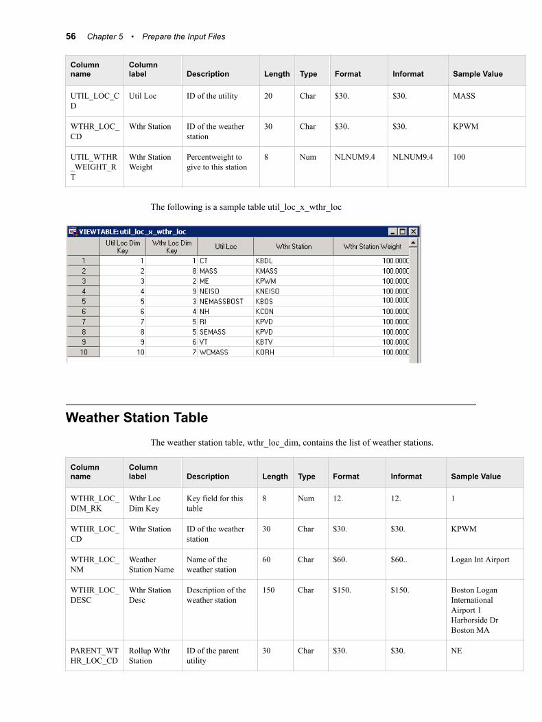
Column name


UTIL_LOC_CD

Util Loc ID of the utility 20 Char $30. $30. MASS

WTHR_LOC_CD

Wthr Station ID of the weather station

30 Char $30. $30. KPWM

UTIL_WTHR_WEIGHT_RT

Wthr Station Weight

Percentweight to give to this station

8 Num NLNUM9.4 NLNUM9.4 100

The following is a sample table util_loc_x_wthr_loc

Weather Station TableThe weather station table, wthr_loc_dim, contains the list of weather stations.

Column name


WTHR_LOC_DIM_RK

Wthr Loc Dim Key


8 Num 12. 12. 1

WTHR_LOC_CD

Wthr Station ID of the weather station

30 Char $30. $30. KPWM

WTHR_LOC_NM

Weather Station Name

Name of the weather station

60 Char $60. $60.. Logan Int Airport

WTHR_LOC_DESC

Wthr Station Desc

Description of the weather station

150 Char $150. $150. Boston Logan International Airport 1 Harborside Dr Boston MA

PARENT_WTHR_LOC_CD

Rollup Wthr Station

ID of the parent utility

30 Char $30. $30. NE


Column name


LONGITUDE_NO

Wthr Station Longitude

Longitude of the weather station

8 Num BEST12. 12. 123

LATITUDE_NO

Wthr Station Latitude

Latitude of the weather station

8 Num BEST12. 12. 123

The following is a sample weather stations table: wthr_loc_dim.

Weather Data TableThe weather data table, wthr_data.sas7bdat, is used as a source data for load forecasting. The temperature data can be several types of data such as Fahrenheit and Centigrade. The type is specified in the field WTHR_TYPE_CD.


WTHR_HR_NO

Hour Ending Hour of reading 8 Num BEST12. 12. 23

WTHR_LOC_DIM_RK

Wthr Loc Dim Key

Record number of the utility in the table UTIL_LOC_DIM

8 Num 12. 12. 1

WTHR_TYPE_CD

Wthr Variable The type of data contained in the column WTHR_NO

15 Char $15. $15. TEMPF

WTHR_DTTM

Datetime Date and Time of reading


WTHR_LOC_CD

Wthr Station Weather station Identifier

30 Char $30. $30. TEMPF

Weather Data Table 57


WTHR_DT Date Month and Day of reading

8 Num NLDATEM14. NLDATE20. 0719

WTHR_NO Wthr Value The reading (e.g., Fahrenheit temperature or Centigrade temperature)

8 Num BEST12. 12. 72

The following is a sample weather table: wthr_data.


Chapter 6

Modify the Parameter Templates

Introduction . . . . . . . . . . . . . . . . . . . . . . . . . . . . . . . . . . . . . . . . . . . . . . . . . . . . . . . . . . 59

PARM_VSTLF . . . . . . . . . . . . . . . . . . . . . . . . . . . . . . . . . . . . . . . . . . . . . . . . . . . . . . . 60

PARM_STLF . . . . . . . . . . . . . . . . . . . . . . . . . . . . . . . . . . . . . . . . . . . . . . . . . . . . . . . . . 61

PARM_MTLTLF . . . . . . . . . . . . . . . . . . . . . . . . . . . . . . . . . . . . . . . . . . . . . . . . . . . . . 61

PARM_VSEL . . . . . . . . . . . . . . . . . . . . . . . . . . . . . . . . . . . . . . . . . . . . . . . . . . . . . . . . 62

IntroductionThe parameters to be displayed on the New Definition dialogs are defined in template files. You can modify these template files, for example, to change the default value of the parameters.

By default, the template files are located in C:\SAS\Config\Lev1\SASApp\Data\EnergyForecasting\Templates.

The following table shows the schema for a template file.

Column Name Type Description

name char (256) The parameter name (e.g. 'utility' or 'weight_num')

value char (256) The parameter value to be used by the forecasting macros (e.g. 'CT')

lbl char (256) The label to be used in the UI (e.g. 'Utility Code'). An attempt to look up localized string using the name parameter occurs first, if found it is used. If one doesn't exist then use lbl.

type char (20) The parameter type, used in the UI to identify the type of input control and format (supported values: char, num, date9)

min num The min value used in the UI for validation when the type is num.

max num The max value used in the UI for validation when the type is num

59

Column Name Type Description

choice char (256) List of choices to be presented in the UI (e.g. mape has the list of choices 'hourly_mape, daily_mape, daily_peak_mape, monthly_mape, monthly_peak_mape, annual_mape, annual_peak_mape'

grp_1 char (30) The first order of grouping used in the UI (tab)

grp_2 char (30) The second order of grouping used in the UI (sub group)

The following template files are supplied on installation of the product:

• “PARM_VSTLF” on page 60

• “PARM_STLF” on page 61

• “PARM_MTLTLF” on page 61

• “PARM_VSEL” on page 62

PARM_VSTLFThe table parm_vstlf contains the parameters for a Foundation very short term load forecast.

Name Label Sample value Type Options

hist_start_date Historical Start Date 01JAN2005 date9 n/a

fcst_start_date Forecast Start Date 01JAN2010 date9 n/a

fcst_start_hour Forecast Start Hour 1 num n/a

fcst_length Forecast Length 24 num n/a

reporting_mart Reporting Mart SAS char SAS, HANA, NONE

reporting_sas_data_model Reporting SAS Data Model Normalized char Normalized, Denormalized, Both

hana_server HANA Server hana.abc.com char n/a

hana_instance HANA Instance 02 char n/a

hana_schema HANA Schema SEFHanaSchema char n/a

hana_authdomain HANA Authentication Domain sefsaphana_auth char n/a

sefvs_init_exit Forecast Initialization Exit C:\sef\init.sas char n/a

sefvs_rpt_exit Reporting Exit C:\sef\report.sas char n/a

60 Chapter 6 • Modify the Parameter Templates


sefvs_term_exit Forecast Completion Exit C:\sef\term.sas char n/a

PARM_STLFThe table parm_stlf contains the parameters for a Foundation short term load forecast.


hist_start_date Historical Start Date 01JAN2005 date9 n/a

fcst_start_date Forecast Start Date 01JAN2010 date9 n/a

fcst_end_date Forecast End Date 07JAN2010 date9 n/a







sefsh_init_exit Forecast Initialization Exit C:\sef\init.sas char n/a

sefsh_rpt_exit Reporting Exit C:\sef\report.sas char n/a

sefsh_term_exit Forecast Completion Exit C:\sef\term.sas char n/a

PARM_MTLTLFThe table parm_mtltlf contains the parameters for a Foundation medium term or long term load forecast.


hist_t_start Historical T Start 01JAN2005 date9 n/a

hist_t_end Historical T End 31DEC2010 date9 n/a

PARM_MTLTLF 61


hist_load_start_dt Historical Load Start Date 01JAN2004 date9 n/a

hist_load_end_dt Historical Load End Date 01JAN2005 date9 n/a

fcst_end_dt Forecast End Date 31DEC2013 date9 n/a

num_scenarios Number of Scenerios 2 num n/a

mtlt_assumption MLT Assumption 1 num n/a







sefml_init_exit Forecast Initialization Exit C:\sef\init.sas char n/a

sefml_rpt_exit Reporting Exit C:\sef\report.sas char n/a

sefml_term_exit Forecast Completion Exit C:\sef\term.sas char n/a

PARM_VSELThe table parm_vsel contains the parameters for a Foundation diagnose.


weight_num Weight 4 num n/a

weight_lower Weight Lower 0.8 num n/a

weight_upper Weight Upper 0.95 num n/a

train_start_date Training Start Date 01JAN2010 date9 n/a

rolling_start_date Rolling Start Date 01JAN2010 date9 n/a

rolling_end_date Rolling End Date 12AUG2013 date9 n/a

sub_hour Sub Hour 7 num n/a



sub_date_offset Sub Date Offset 1 num n/a

mape MAPE hourly_mape char hourly_mape

daily_mape

daily_peak_mape

monthly_mape

monthly_peak_mape

annual_mape

annual_peak_mape

w_hourly_mape Weight Hourly MAPE 0.25 num n/a

w_daily_mape Weight Daily MAPE 0.25 num n/a

w_daily_peak_mape Weight Daily Peak MAPE 0 num n/a

w_monthly_mape Weight Monthly MAPE 0.25 num n/a

w_monthly_peak_mape Weight Monthly Peak MAPE 0 num n/a

w_annual_mape Weight Annual MAPE 0.25 num n/a

w_annual_peak_mape Weight Annual Peak MAPE 0 num n/a

mape_improvement Mape Improvement 0.0001 num n/a

outlier_percent Outlier Percent 0.001 num n/a

residual_hist_length Residual History Length 504 num n/a

combine_fcst Combine Forecast 1234 char n/a

poly_order Poly Order 3 num n/a

ape_cutoff APE Cutoff 0.3 num n/a

two_stage Two Stage YES char YES, NO

default_wthr_type_cd Default Weather Type Code TEMPF char n/a

wls WLS YES char YES, NO

add_var Additional Modeling Variables wind humidity char n/a

add_class Additional Class Variables MONTH WEEKDAY

char n/a

utility Utility Code UNITEDILL char n/a

num_cpu Number of CPUs 8 num n/a

staged_data_path Input Path N:/ULF/Data/Staged

char n/a

PARM_VSEL 63


data_model Data Model 3.1 char 3.1, 2

fix_date_holiday_list Fixed Date Holidays 1 5 8 10 char n/a

sefdg_init_exit Diagnose Initialization Exit C:\sef\init.sas char n/a

sefdg_term_exit Diagnose Completion Exit C:\sef\term.sas char n/a


Chapter 7

Modify Application Settings

Application Settings . . . . . . . . . . . . . . . . . . . . . . . . . . . . . . . . . . . . . . . . . . . . . . . . . . . 65

Application SettingsTo modify SAS Energy Forecasting settings:

1. Open SAS Management Console as an administrator.

2. On the Plug-ins tab, right-click Application Management ð Configuration Manager ð SAS Application Infrastructure ð Energy Forecasting Server 3.1 and select Properties.

The Energy Forecasting Properties window opens.

3. Click the Settings tab.

4. On the left-hand side of the Properties window, select Energy Forecasting.

5. Select and modify the properties that you want.

65

66 Chapter 7 • Modify Application Settings

Chapter 8

Add Additional Variables as Parameters

Overview . . . . . . . . . . . . . . . . . . . . . . . . . . . . . . . . . . . . . . . . . . . . . . . . . . . . . . . . . . . . 67

Supply a Data Set with the Additional Variables and Their Data . . . . . . . . . . . . . . 67

Specify the Additional Variables as Parameters in the UI . . . . . . . . . . . . . . . . . . . . 68

OverviewBy default, SAS Energy Forecasting uses the load history and temperature history to predict what the demand load is going to be in the future. For medium/long term forecasting, it also uses economic scenarios. However, you can include additional variables as independent variables/effects in the prediction process. For example, you can include variables for humidity, customer counts, etc. To include additional variables, you must:

1. “Supply a Data Set with the Additional Variables and Their Data” on page 67

2. “Specify the Additional Variables as Parameters in the UI” on page 68

Supply a Data Set with the Additional Variables and Their Data

The data set containing the additional variables and their data must be a standard SAS data set named user_defined_data. It must contain a datetime column; and the range of dates must be consistent with other incoming data. It can contain one or more numeric variables to be used as additional variables. For more information, see “User-Defined Data Table” on page 53.

The following picture shows a sample data set.

67

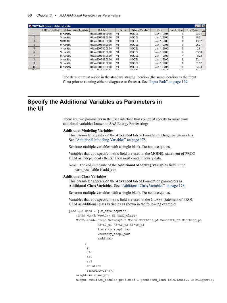
The data set must reside in the standard staging location (the same location as the input files) prior to running either a diagnose or forecast. See “Input Path” on page 179.

Specify the Additional Variables as Parameters in the UI

There are two parameters in the user interface that you must specify to make your additional variables known to SAS Energy Forecasting:

Additional Modeling VariablesThis parameter appears on the Advanced tab of Foundation Diagnose parameters. See “Additional Modeling Variables” on page 178.

Separate multiple variables with a single blank. Do not use quotes.

Variables that you specify in this field are used in the MODEL statement of PROC GLM as independent effects. They must contain hourly data.

Note: The column name of the Additional Modeling Variables field in the parm_vsel table is add_var.

Additional Class VariablesThis parameter appears on the Advanced tab of Foundation parameters as Additional Class Variables. See “Additional Class Variables” on page 178.


Variables that you specify in this field are used in the CLASS statement of PROC GLM as additional class variables as shown in the following example:

proc GLM data = glm_data noprint; CLASS Month Weekday HE &add_class; MODEL load= trend Weekday*HE Month Month*t0_p1 Month*t0_p2 Month*t0_p3 HE*t0_p1 HE*t0_p2 HE*t0_p3 &recency_step2_var &recenty_step3_var &add_var / p clm ss1 ss3 solution SINGULAR=1E-07; weight &wls_weight; output out=fcst_results predicted = predicted_load lclm=lower95 uclm=upper95;

68 Chapter 8 • Add Additional Variables as Parameters

run;quit;

Note: The column name of the Additional Class Variables field in the parm_vsel table is add_class.

Specify the Additional Variables as Parameters in the UI 69

70 Chapter 8 • Add Additional Variables as Parameters

Chapter 9

Archive Results Data

Overview . . . . . . . . . . . . . . . . . . . . . . . . . . . . . . . . . . . . . . . . . . . . . . . . . . . . . . . . . . . . 71

Macro %sefarche . . . . . . . . . . . . . . . . . . . . . . . . . . . . . . . . . . . . . . . . . . . . . . . . . . . . . 72Overview . . . . . . . . . . . . . . . . . . . . . . . . . . . . . . . . . . . . . . . . . . . . . . . . . . . . . . . . . . 72Syntax . . . . . . . . . . . . . . . . . . . . . . . . . . . . . . . . . . . . . . . . . . . . . . . . . . . . . . . . . . . . 72ENCF.Archive.path . . . . . . . . . . . . . . . . . . . . . . . . . . . . . . . . . . . . . . . . . . . . . . . . . . 74

Specify Files to Archive by Date . . . . . . . . . . . . . . . . . . . . . . . . . . . . . . . . . . . . . . . . . 75

Specify Files to Archive by Name . . . . . . . . . . . . . . . . . . . . . . . . . . . . . . . . . . . . . . . . 76

Specify Files to Archive by Name and Date . . . . . . . . . . . . . . . . . . . . . . . . . . . . . . . . 78

OverviewSAS Energy Forecasting is very data intensive—it uses large amounts of data and generates large amounts of data. Unless you systematically clean up your result data sets, you risk using up your disk space. SAS Energy Forecasting provides methods to archive your forecasting and diagnose results so that you can:

• free up sufficient disk space for the application to run

• preserve selected result data so that you can justify your forecasting to regulatory bodies.

To archive data, run the SAS macro %sefarche on the data tier to signal SAS Energy Forecasting to archive result data.

By default, all the results folders are archived for every diagnose and forecast definition in every project. However, you can limit what is archived. See the following:

• “Specify Files to Archive by Date” on page 75

• “Specify Files to Archive by Name” on page 76

• “Specify Files to Archive by Name and Date” on page 78

As part of archiving, when a results folder is archived the following folders are deleted:

• the results folder itself

• the parent folder of the results folder

• the sibling folders of the results folder (sources and work)

All that remains by default are the archived files in the archive location and the diagnose and forecast definitions. The following picture shows one diagnose results folder and

71

one forecast results folders being archived. The parent folders of the results folders are deleted along with the results siblings. The diagnose and forecast definitions are not touched by the archiving.

Only diagnose result files and forecast result files whose state is SUCCESS or COMPLETE_WARNING are archived. If an error is encountered during archiving, then a file whose status was SUCCESS is not archived and its status is changed to ARCHIVE_PENDING. And a file whose status was COMPLETE_WARNING is not archived and its status is changed to ARCHIVE_PENDING_WARNING. The next time archiving takes place, files in either PENDING state are attempted to be archived. If the archiving is successful, then the file status is changed back to SUCCESS and COMPLETE_WARNING respectively (in its archived location).

Macro %sefarche

OverviewRun the SAS macro %sefarche on the data tier to signal SAS Energy Forecasting to archive your result data. Only one instance of the macro can run at a time.

SyntaxThe syntax of the macro is the following:

%sefarche(archive_path=<base_path>);

where the value of archive_path= is a complete file path. For example:

%sefarche(archive_path=C:\sef_archive;

The file path that you specify can be local to the data tier or it can be on a remote machine that is accessible by the data tier. The file path is the base path for archiving.

Note:

• The parameter archive_path= is optional. You can also specify an archive path by specifying the property, ENFC.Archive.path, in SAS Management Console. See “ENCF.Archive.path” on page 74. If ENFC.Archive.path is specified, then if you also specify the parameter archive_path= the parameter overrides ENFC.Archive.path.

72 Chapter 9 • Archive Results Data

• Make sure that the user Energy Forecasting Server User has permission to write to the directories that are created by the archiving process. The user Energy Forecasting Server User is created upon installation of SAS Energy Forecasting. On a Windows system, you grant permission by right-clicking a folder and selecting Properties. Then click the Security tab.

• Make sure, also, that the user Energy Forecasting Server User has the following capabilities:

• Delete Diagnose Results

• Delete Forecast Results

• Energy Forecasting User

See “Create Roles” on page 32.

The archiving process creates the following subdirectories under this base path:

Diagnose archive subdirectoriesFor each diagnose that is archived, a subdirectory is created using the following naming convention:

<base_path>\project_name\diagnose_definition_name\diagnose_results_name

For example: C:\SEF_Archive\Project_1\Proj1_CT_Diag_1\20141002_150801.

The following picture shows a sample diagnose archive subdirectory whose base path is C:\SEF_Archive.

Forecast archive subdirectoriesFor each forecast that is archived, a subdirectory is created using the following naming convention:

<base_path>\project_name\forecast_definition_name\forecast_results_name

For example: C:\SEF_Archive\Project_1_CT_Diag_1\Proj1_CT_VSTLF_1\20141002_172617.

The following picture shows a sample forecast archive subdirectory whose base path is C:\SEF_Archive.

Macro %sefarche 73

ENCF.Archive.pathYou can specify an archive path by specifying the metadata property ENFC.Archive.path in SAS Management Console. To set the property:

1. Open SAS Management Console as an administrator.

2. On the Plug-ins tab, right-click Application Management ð Configuration Manager ð SAS Application Infrastructure ð Energy Forecasting 3.1 and select Properties.

The Energy Forecasting Properties window opens.

3. Select the Advanced tab, and then do one of the following:

• If the ENFC.Archive.path property does not exist, then:

1. click Add.

The Define New Property window opens.

2. On the Define New Property window, specify the following:

Property NameSpecify ENFC.Archive.path

Property ValueSpecify a complete path. The file path that you specify can be local to the data tier or it can be on a remote machine that is accessible by the data tier. The file path is the base path for archiving.

Note: You must restart the data tier server for the change to take effect.


• If the ENFC.Archive.path property already exists, then specify a complete path as its Property Value.The file path that you specify can be local to the data tier or it can be on a remote machine that is accessible by the data tier. The file path is the base path for archiving.

Specify Files to Archive by DateYou can control which result files are archived by specifying how old they must be to be archived. To control what files are archived, you modify settings with SAS Management

Specify Files to Archive by Date 75

Console. For information on modifying these settings, see “Application Settings” on page 65. The settings are the following::

Keep this number of diagnose resultsSpecifies how many of the most recent diagnose results are to be kept—the rest are archived and then deleted. For example, suppose you enter 2. Then for each diagnose definition, results that are older than the 2 most recent results are archived and deleted. For example, as the following picture shows:

• the two newest diagnose results are left alone

• one older one is archived (that is, its results folder is archived)

• and it is deleted (that is, its parent folder is deleted along with its children—the results, sources, and work folders.

Archive MTLT forecast results older than this many weeksSpecifies how many weeks old a medium term/long term forecast must be to be archived. For example, suppose you enter 8. Then, for each MTLTLF definition, all of its forecast results that are older than 8 weeks are archived—that is, the results folder is archived. And it is deleted—that is, its parent folder is deleted along with its children (the results, sources, and work folders).

Archive ST forecast results older than this many daysSpecifies how many days old a short term forecast must be to be archived. For example, suppose you enter 6, Then, for each STLF definition, all of its forecast results that are older than 6 days are archived—(that is, the results folder is archived. And it is deleted—that is, its parent folder is deleted along with its children (the results, sources, and work folders).

Archive VST forecast results older than this many hoursSpecifies how many hours old a very short term forecast result must be to be archived. For example, suppose you enter 4. Then, for each VSTLF definition, all of its forecast results that are older than 4 hours are archived—that is, the results folder is archived. And it is deleted—that is, its parent folder is deleted along with its children (the results, sources, and work folders).

Specify Files to Archive by NameYou can create SAS data sets to specify by name what files are to be archived. The data sets must be named as follows:

archive_diagnose.sas7bdatSpecifies diagnose files to archive.

archive_vstlf.sas7bdatSpecifies very short term load forecasting files to archive.


archive_stlf.sas7bdatSpecifies short term load forecasting files to archive.

archive_mtltlf.sas7bdatSpecifies medium term/long term load forecasting files to archive.

The SAS data sets must contain the following columns:

Column Name Column Contents

sub_dir Each row in this column must contain one of the four following string values:

resultsDesignates files in the results subdirectory,

sourcesDesignates files in the sources subdirectory,

workDesignates files in the work subdirectory,

sas null data set value (.)Designates files in the base directory.

filename Each row in this column contains a string that matches the name of a file to be archived. The file specified must be in the directory specified in the corresponding sub_dir column. You must specify the full filename including the file extension, for example .sas7bdat.

There is a set of sample data sets for you to look at and modify. On Windows, they are in the SAS Home directory—for example C:\Program Files\SAS Home\SASFoundation\9.4\enfcsvr\sample. For further information, refer to the SAS Energy Forecasting Installation Guide available at http://support.sas.com/documentation/solutions/ef/.

At run time, these data sets must reside in the same directory as the parameter template files. On Windows, for example, in C:\SAS\Config\Lev1\AppData\SASEnergyForecasting\templates. See Chapter 6, “Modify the Parameter Templates,” on page 59.

The following picture shows a sample SAS data set, archive_diagnose.

This sample data set specifies the following:

• In the sources directory, archive the following two files:

• wthr_data.sas7bdat

• load_data.sas7bdat

• In the base directory (null in the sub_dir field), archive the file messages.sas7bdat.

• In the results directory, archive the following two files:

Specify Files to Archive by Name 77

• fcst_results_all.sas7bdat

• fcst_results.sas7bdat

• In the work directory, archive the file economy.sas7bdat.

Also, as part of the archiving, the parent folder is deleted along with its children folders—the results, sources, and work folders.

Specify Files to Archive by Name and DateYou can combine specifications of name and date so as to archive specifically named files whose date is older than your specified criterion. For example, suppose that you enter

ENFC.DIAGNOSE.ArchiveCutoff=2

so as to archive only diagnoses that are older than the two most recent ones. And, suppose also that you provide the data set archive_diagnose.sas7bdat to specify that only fcst_results.sas7bdat in the results folder should be archived. Then, if as shown in the following picture, there exist four diagnose results altogether, only the two files, fcst_results.sas7bdat, from the two older diagnose results are archived.


Chapter 10

Run in Batch

Overview . . . . . . . . . . . . . . . . . . . . . . . . . . . . . . . . . . . . . . . . . . . . . . . . . . . . . . . . . . . . 79

Macro %sefdatae . . . . . . . . . . . . . . . . . . . . . . . . . . . . . . . . . . . . . . . . . . . . . . . . . . . . . 79

Examples . . . . . . . . . . . . . . . . . . . . . . . . . . . . . . . . . . . . . . . . . . . . . . . . . . . . . . . . . . . . 80

OverviewWithout opening the SAS Energy Forecasting client, you can use the macro %sefdatae on the data tier to run forecasts for which the property Enable Event Listening has been selected. The parameters of the %sefdatae macro specify exactly which forecasts to run.

Typically, you might run the macro after updating input data for a forecast.

You can select Enable Event Listening for any forecast.

Macro %sefdatae%sefdatae(

utility=utility_code

, stage_path=input_path

, forecast_type=VSTLF | STLF | MTLTLF

, name_regexp=input_path

);

79

utility=Required. A forecast is run only if its definition contains this utility code. The macro can run multiple forecasts in multiple projects if the forecast definitions share the same utility code.

stage_path=Required. The complete path for the input files. See “Input Path” on page 179.

forecast_type=Optional. Valid values are:

VSTLF Very Short Term Load Forecasting

STLF Short Term Load Forecasting

MTLTLF Medium Term/Long Term Load Forecasting

If you don’t specify this parameter, then all types of forecast are run.

name_regexp=Optional. A java regular expression to match a forecast name. A forecast is run only if its name matches this regular expression.

Examples of regular expressions are:

• HOURLY$ matches names that end in HOURLY, such as CT_VSTL_HOURLY

• ^HOURLY matches names that begin with HOURLY, such as HOURLY_CT_VSLT.

• HOURLY and _HOURLY_ both match names that include HOURLY, such as CT_HOURLY_VSLT.

The following restrictions apply:

• The following characters are not allowed:

< > ( ) , \N \V \R

• You may not use any character or sequence of characters that is not valid as an XML attribute.

• You may not use any character or sequence of characters that cannot be included in a SAS macro variable.

Examples• %sefdatae(utility=mass, stage_path=C:\ULF\Data\mass\stage);

Runs all forecast definitions defined for the region mass and using the input files at the location C:\ULF\Data\mass\stage

• %sefdatae(utility=ct, stage_path=C:\ULF\Data\ct\stage, forecast_type=VSTLF);

Runs all very short term forecast definitions defined for the region ct and using the input files at the location C:\ULF\Data\ct\stage

• %sefdatae(utility=ct, stage_path=C:\ULF\Data\ct\stage, forecast_type=STLF);

Runs all short term forecast definitions defined for the region ct and using the input files at the location C:\ULF\Data\ct\stage

• %sefdatae(utility=ct, stage_path=C:\ULF\Data\ct\stage, name_regexp=HOURLY$,

80 Chapter 10 • Run in Batch

forecast_type=VSTLF);

Runs all very short term forecast definitions defined for the region ct whose name end with HOURLY. Use input files at the location C:\ULF\Data\ct\stage

Examples 81

82 Chapter 10 • Run in Batch

Chapter 11

Produce Reports

Overview . . . . . . . . . . . . . . . . . . . . . . . . . . . . . . . . . . . . . . . . . . . . . . . . . . . . . . . . . . . . 83

Normalized Tables . . . . . . . . . . . . . . . . . . . . . . . . . . . . . . . . . . . . . . . . . . . . . . . . . . . . 84Introduction . . . . . . . . . . . . . . . . . . . . . . . . . . . . . . . . . . . . . . . . . . . . . . . . . . . . . . . . 84VSTLF . . . . . . . . . . . . . . . . . . . . . . . . . . . . . . . . . . . . . . . . . . . . . . . . . . . . . . . . . . . 84STLF . . . . . . . . . . . . . . . . . . . . . . . . . . . . . . . . . . . . . . . . . . . . . . . . . . . . . . . . . . . . . 88MTLF/LTLF . . . . . . . . . . . . . . . . . . . . . . . . . . . . . . . . . . . . . . . . . . . . . . . . . . . . . . . 92

Denormalized SAS Data Sets . . . . . . . . . . . . . . . . . . . . . . . . . . . . . . . . . . . . . . . . . . . . 96Introduction . . . . . . . . . . . . . . . . . . . . . . . . . . . . . . . . . . . . . . . . . . . . . . . . . . . . . . . . 96VSTLF . . . . . . . . . . . . . . . . . . . . . . . . . . . . . . . . . . . . . . . . . . . . . . . . . . . . . . . . . . . 97STLF . . . . . . . . . . . . . . . . . . . . . . . . . . . . . . . . . . . . . . . . . . . . . . . . . . . . . . . . . . . . 100MTLF/LTLF . . . . . . . . . . . . . . . . . . . . . . . . . . . . . . . . . . . . . . . . . . . . . . . . . . . . . . 103

OverviewWith SAS Energy Forecasting, you can output tables that are suitable for producing reports using SAS Visual Analytics or HANA or another report tool. You can output two types of tables:

Normalized TablesIf you select normalized output, then you get more (but smaller) tables without redundant data than you do with denormalized output where you get fewer (but larger) tables with redundant data. Normalized tables require you to do joins on the tables for reporting.

If you are using HANA as your reporting tool, then you must use normalized tables. The normalized tables are outputted as HANA tables.

See “Normalized Tables” on page 84.

Denormalized Data SetsIf you select denormalized output, then you get fewer (but larger) tables with redundant data than you do with normalized output where you get more (but smaller) tables without redundant data.

Denormalized tables are outputted as SAS data sets. If you are using SAS Visual Analytics as your reporting tool, then you can use either normalized or denormalized tables. If you are using another reporting tool, you might want to use either denormalized or normalized tables depending on the tool.

83

T I P Particularly if you output denormalized tables, the storage required can become very large. Make sure that you periodically purge these data sets so as to free up space.

See “Denormalized SAS Data Sets” on page 96.

Normalized Tables

IntroductionIf you are using HANA as your reporting tool, then you must use normalized tables.

The location to which normalized tables are written is based on the following order of precedence:

1. If you pre-allocated a libref named freport, then SAS Energy Forecasting uses that.

2. If you defined a library named freport of type HANA in the metadata server, then SAS Energy Forecasting uses that.

VSTLF

SummaryFollowing tables:

• CALENDAR (replaced)

• RUN_INFORMATION (appended to)

• USER_DEFINED_DATA (appended to)(optional)

• VSTLF_FCST_RESULTS (appended to)

• VSTLF_FCST_STAT (appended to)

• VSTLF_OUTLIER (appended to)

• WTHR_DATA (appended to)

CALENDARThe CALENDAR table is replaced each time a forecast is run. It contains the following columns:

Column Name

UTIL_LOC_CD (key)

DATE (key)

HOLIDAY

BEFORE_HOLIDAY

AFTER_HOLIDAY

84 Chapter 11 • Produce Reports

Column Name

YEAR

MONTH

DAY

WEEKDAY

RUN_INFORMATIONThe RUN_INFORMATION table is appended to each time a forecast is run. It contains the following columns:

Column Name

RUN_ID_NM (key)

RUN_TYPE_CD (key)

RUN_ID_DTTM

UTIL_LOC_CD

RUN_ID_DESC

WTHR_LOC_CD

WTHR_LOC_NM

WTHR_LOC_DESC

UTIL_LOC_NM

UTIL_LOC_DESC

USER_DEFINED_DATAThe USER_DEFINED_DATA table is optional. If it exists, it is appended to each time a forecast is run. It contains the following columns:

Column Name

UD_DTTM (key)

UD_TYPE_COL_NM (key)

RUN_ID_NM (foreign key)

RUN_TYPE_CD (foreign key)

Normalized Tables 85

Column Name

UD_TYPE_CD

UD_DT

UD_HR_NO

UD_NO

VSTLF_FCST_RESULTSThe VSTLF_FCST_RESULTS table is appended to each time a forecast is run. It contains the following columns:

Column Name

VSTLF_FCST_RESULTS_DTTM (key)

VSTLF_MODEL_NM (key)



VSTLF_FCST_RESULTS_DT

VSTLF_FCST_RESULTS_HR_NO

VSTLF_PREDICTED_LOAD_NO

CHAMPION_FLG

VSTLF_FCST_STATThe VSTLF_FCST_STAT table is appended to each time a forecast is run. It contains the following columns:

Column Name




VSTLF_HOURLY_ME_NO

VSTLF_HOURLY_MAE_NO

VSTLF_HOURLY_MAPE_NO


Column Name

VSTLF_DAILY_PEAK_ME_NO

VSTLF_DAILY_PEAK_MAE_NO

VSTLF_DAILY_PEAK_MAPE_NO

VSTLF_DAILY_ME_NO

VSTLF_DAILY_MAE_NO

VSTLF_DAILY_MAPE_NO

VSTLF_MONTHLY_PEAK_ME_NO

VSTLF_MONTHLY_PEAK_MAPE_NO

VSTLF_MONTHLY_PEAK_MAE_NO

VSTLF_MONTHLY_ME_NO

VSTLF_MONTHLY_MAPE_NO

VSTLF_MONTHLY_MAE_NO

VSTLF_ANNUAL_PEAK_ME_NO

VSTLF_ANNUAL_PEAK_MAE_NO

VSTLF_ANNUAL_PEAK_MAPE_NO

VSTLF_ANNUAL_ME_NO

VSTLF_ANNUAL_MAE_NO

VSTLF_ANNUAL_MAPE_NO

VSTLF_WEIGHTED_MAPE_NO

VSTLF_OUTLIERThe VSTLF_OUTLIER table is appended to each time a forecast is run. It contains the following columns:

Column Name

VSTLF_OUTLIER_DTTM (key)

VSTLF_OUTLIER_TYPE_CD (key)


Column Name



VSTLF_WEEK_DAY_NO

VSTLF_WEEK_DAY_ORIG_NO

VSTLF_SPECIAL_DAY_NO

VSTLF_WTHR_NO

VSTLF_WTHR_TYPE_CD

VSTLF_ACTUAL_LOAD_NO


VSTLF_ERROR_NO

VSTLF_ABS_ERROR_NO

VSTLF_ABS_ERROR_PCT

WTHR_DATAThe WTHR_DATA table is appended to each time a forecast is run. It contains the following columns:

Column Name

WTHR_DTTM (key)



WTHR_HR_NO

WTHR_TYPE_CD

WTHR_NO

STLF





• STLF_FCST_RESULTS (appended to)

• STLF_FCST_STAT (appended to)




Column Name

UTIL_LOC_CD (key)

DATE (key)

HOLIDAY

BEFORE_HOLIDAY

AFTER_HOLIDAY

YEAR

MONTH

DAY

WEEKDAY


Column Name

RUN_ID_NM (key)

RUN_TYPE_CD (key)

RUN_ID_DTTM

UTIL_LOC_CD

RUN_ID_DESC

WTHR_LOC_CD


Column Name

WTHR_LOC_NM

WTHR_LOC_DESC

UTIL_LOC_NM

UTIL_LOC_DESC

STLF_FCST_RESULTSThe STLF_FCST_RESULTS table is appended to each time a forecast is run. It contains the following columns:

Column Name

STLF_FCST_RESULTS_DTTM (key)

STLF_MODEL_NM (key)

STLF_FCST_WTHR_TYPE_CD RUN_ID_NM (foreign key)


STLF_FCST_RESULTS_DT

STLF_FCST_RESULTS_HR_NO

STLF_PREDICTED_LOAD_NO

STLF_FCST_WTHR_NO

CHAMPION_FLG

STLF_FCST_STATThe STLF_FCST_STAT table is appended to each time a forecast is run. It contains the following columns:

Column Name

STLF_MODEL_NM (key)



CHAMPION_FLG

STLF_HOURLY_ME_NO


Column Name

STLF_HOURLY_MAE_NO

STLF_HOURLY_MAPE_NO

STLF_DAILY_PEAK_ME_NO

STLF_DAILY_PEAK_MAE_NO

STLF_DAILY_PEAK_MAPE_NO

STLF_DAILY_ME_NO

STLF_DAILY_MAE_NO

STLF_DAILY_MAPE_NO

STLF_MONTHLY_PEAK_ME_NO

STLF_MONTHLY_PEAK_MAPE_NO

STLF_MONTHLY_PEAK_MAE_NO

STLF_MONTHLY_ME_NO

STLF_MONTHLY_MAPE_NO

STLF_MONTHLY_MAE_NO

STLF_ANNUAL_PEAK_ME_NO

STLF_ANNUAL_PEAK_MAE_NO

STLF_ANNUAL_PEAK_MAPE_NO

STLF_ANNUAL_ME_NO

STLF_ANNUAL_MAE_NO

STLF_ANNUAL_MAPE_NO

STLF_WEIGHTED_MAPE_NO



Column Name

UD_DTTM (key)




UD_TYPE_CD

UD_DT

UD_HR_NO

UD_NO


Column Name

WTHR_DTTM (key)



WTHR_HR_NO

WTHR_TYPE_CD

WTHR_NO

MTLF/LTLF



• ECONOMY_DATA (appended to)

• MTLTLF_FCST_RESULTS (appended to)

• MTLTLF_PEAK_STAT (appended to)






Column Name

UTIL_LOC_CD (key)

DATE (key)

HOLIDAY

BEFORE_HOLIDAY

AFTER_HOLIDAY

YEAR

MONTH

DAY

WEEKDAY

ECONOMY_DATAThe ECONOMY_DATA table is appended to each time a forecast is run. It contains the following columns:

Column Name

ECONOMY_DT (key)

RUN_ID_NM (foreign key))

RUN_TYPE_CD (foreign key))









MTLTLF_FCST_RESULTSThe MTLTLF_FCST_RESULTS table is appended to each time a forecast is run. It contains the following columns:

Column Name

MTLTLF_FCST_RESULTS_DTTM (key)

MTLTLF_MODEL_NM (key)

MTLTLF_MODEL_ECONOMIC_SCN_NO (key)

MTLTLF_RESULTS_YEAR_ORIG_NO (key)


RUN_TYPE_CD (foreign key))

MTLTLF_FCST_RESULTS_DT

MTLTLF_FCST_RESULTS_HR_NO

MTLTLF_RESULTS_YEAR_NO

MTLTLF_ACTUAL_LOAD_NO

MTLTLF_PREDICTED_LOAD_NO

MTLTLF_PEAK_STATThe MTLTLF_PEAK_STAT table is appended to each time a forecast is run. It contains the following columns:

Column Name

MTLTLF_PEAK_YR_NO (key)



RUN_ID_NM ( foreign key)


MTLTLF_PEAK_NO

MTLTLF_PEAK_MIN_NO

MTLTLF_PEAK_P10_NO


Column Name

MTLTLF_PEAK_ME_NO

MTLTLF_PEAK_MED_NO

MTLTLF_PEAK_P90_NO

MTLTLF_PEAK_MAX_NO

MTLTLF_PEAK_ACTUAL_NO


Column Name

RUN_ID_NM (key)

RUN_TYPE_CD (key)

RUN_ID_DTTM

UTIL_LOC_CD

RUN_ID_DESC

WTHR_LOC_CD

WTHR_LOC_NM

WTHR_LOC_DESC

UTIL_LOC_NM

UTIL_LOC_DESC


Column Name

UD_DTTM (key)




Column Name


UD_TYPE_CD

UD_DT

UD_HR_NO

UD_NO


Column Name

WTHR_DTTM (key)



WTHR_HR_NO

WTHR_TYPE_CD

WTHR_NO

Denormalized SAS Data Sets

IntroductionIf you are using SAS Visual Analytics as your reporting tool, then you can use either normalized or denormalized tables.

The location to which denormalized tables are written is based on the following order of precedence:

1. If you have pre-allocated a libref named freport, then SAS Energy Forecasting uses that.

2. If you have created a library named freport in the metadata server, then SAS Energy Forecasting uses that.

3. Otherwise, SAS Energy Forecasting creates a folder named rptdata in the data mart.


VSTLF

OverviewFollowing tables:



• VSTLF_FCST_RESULTS_MAST (appended to)


Column Name

UTIL_LOC_CD (key)

DATE (key)

HOLIDAY

BEFORE_HOLIDAY

AFTER_HOLIDAY

YEAR

MONTH

DAY

WEEKDAY


Column Name

RUN_ID_NM (key)

RUN_TYPE_CD (key)

RUN_ID_DTTM

UTIL_LOC_CD

RUN_ID_DESC

Denormalized SAS Data Sets 97

Column Name

WTHR_LOC_CD

WTHR_LOC_NM

WTHR_LOC_DESC

UTIL_LOC_NM

UTIL_LOC_DESC

VSTLF_FCST_RESULTS_MASTThe VSTLF_FCST_RESULTS_MAST table is appended to each time a forecast is run. It contains the following columns:

Column Name





VSTLF_FCST_RESULTS_DT

VSTLF_FCST_RESULTS_HR_NO


VSTLF_HOURLY_ME_NO

VSTLF_HOURLY_MAE_NO

VSTLF_HOURLY_MAE_NO

VSTLF_HOURLY_MAPE_NO

VSTLF_DAILY_PEAK_ME_NO

VSTLF_DAILY_PEAK_MAE_NO

VSTLF_DAILY_PEAK_MAPE_NO

VSTLF_DAILY_ME_NO

VSTLF_DAILY_MAE_NO


Column Name

VSTLF_DAILY_MAPE_NO

VSTLF_MONTHLY_PEAK_ME_NO

VSTLF_MONTHLY_PEAK_MAPE_NO

VSTLF_MONTHLY_PEAK_MAE_NO

VSTLF_MONTHLY_ME_NO

VSTLF_MONTHLY_MAPE_NO

VSTLF_MONTHLY_MAE_NO

VSTLF_ANNUAL_PEAK_ME_NO

VSTLF_ANNUAL_PEAK_MAE_NO

VSTLF_ANNUAL_PEAK_MAPE_NO

VSTLF_ANNUAL_ME_NO

VSTLF_ANNUAL_MAE_NO

VSTLF_ANNUAL_MAPE_NO

VSTLF_WEIGHTED_MAPE_NO

VSTLF_WEEK_DAY_NO

VSTLF_WEEK_DAY_ORIG_NO

VSTLF_SPECIAL_DAY_NO

VSTLF_ACTUAL_LOAD_NO

VSTLF_ERROR_NO

VSTLF_ABS_ERROR_NO

VSTLF_ABS_ERROR_PCT

UD_TYPE_CD

UD_NO

UD_TYPE_COL_NM

WTHR_TYPE_CD


Column Name

UTIL_LOC_CD

WTHR_NO

RUN_ID_DESC

WTHR_LOC_CD

WTHR_LOC_NM

WTHR_LOC_DESC

UTIL_LOC_NM

UTIL_LOC_DESC

CHAMPION_FLG

STLF




• STLF_FCST_RESULTS_MAST (appended to)


Column Name

UTIL_LOC_CD (key)

DATE (key)

HOLIDAY

BEFORE_HOLIDAY

AFTER_HOLIDAY

YEAR

MONTH


Column Name

DAY

WEEKDAY


Column Name

RUN_ID_NM (key)

RUN_TYPE_CD (key)

RUN_ID_DTTM

UTIL_LOC_CD

RUN_ID_DESC

WTHR_LOC_CD

WTHR_LOC_NM

WTHR_LOC_DESC

UTIL_LOC_NM

UTIL_LOC_DESC

STLF_FCST_RESULTS_MASTThe STLF_FCST_RESULTS_MAST table is appended to each time a forecast is run. It contains the following columns:

Column Name





STLF_FCST_RESULTS_DT

STLF_FCST_RESULTS_HR_NO


Column Name

STLF_PREDICTED_LOAD_NO

STLF_WEEK_DAY_NO

STLF_WEEK_DAY_ORIG_NO

STLF_ACTUAL_LOAD_NO

STLF_ERROR_NO

STLF_ABS_ERROR_NO

STLF_ABS_ERROR_PCT

STLF_SPECIAL_DAY_NO

STLF_OUTLIER_FLG

STLF_HOURLY_ME_NO

STLF_HOURLY_MAE_NO

STLF_HOURLY_MAPE_NO

STLF_DAILY_PEAK_ME_NO

STLF_DAILY_PEAK_MAE_NO

STLF_DAILY_PEAK_MAPE_NO

STLF_DAILY_ME_NO

STLF_DAILY_MAE_NO

STLF_DAILY_MAPE_NO

STLF_MONTHLY_PEAK_ME_NO

STLF_MONTHLY_PEAK_MAPE_NO

STLF_MONTHLY_PEAK_MAE_NO

STLF_MONTHLY_ME_NO

STLF_MONTHLY_MAPE_NO

STLF_MONTHLY_MAE_NO

STLF_ANNUAL_PEAK_ME_NO


Column Name

STLF_ANNUAL_PEAK_MAE_NO

STLF_ANNUAL_PEAK_MAPE_NO

STLF_ANNUAL_ME_NO

STLF_ANNUAL_MAE_NO

STLF_ANNUAL_MAPE_NO

STLF_WEIGHTED_MAPE_NO

UD_NO

UD_TYPE_COL_NM

UTIL_LOC_CD

WTHR_TYPE_CD

WTHR_NO

RUN_ID_DESC

WTHR_LOC_CD

WTHR_LOC_NM

WTHR_LOC_DESC

UTIL_LOC_NM

UTIL_LOC_DESC

CHAMPION_FLG

MTLF/LTLF




• MTLTLF_FCST_RESULTS_MAST (appended to)



Column Name

UTIL_LOC_CD (key)

DATE (key)

HOLIDAY

BEFORE_HOLIDAY

AFTER_HOLIDAY

YEAR

MONTH

DAY

WEEKDAY


Column Name

RUN_ID_NM (key)

RUN_TYPE_CD (key)

RUN_ID_DTTM

UTIL_LOC_CD

RUN_ID_DESC

WTHR_LOC_CD

WTHR_LOC_NM

WTHR_LOC_DESC

UTIL_LOC_NM

UTIL_LOC_DESC


MTLTLF_FCST_RESULTS_MASTThe MTLTLF_FCST_RESULTS_MAST table is appended to each time a forecast is run. It contains the following columns:

Column Name

MTLTLF_FCST_RESULTS_DTTM (key)



MTLTLF_RESULTS_YEAR_ORIG_NO (key)

RUN_ID_NM (foreign key))


MTLTLF_FCST_RESULTS_DT

MTLTLF_FCST_RESULTS_HR_NO

MTLTLF_RESULTS_YEAR_NO

MTLTLF_ACTUAL_LOAD_NO

MTLTLF_PREDICTED_LOAD_NO

MTLTLF_PEAK_NO

MTLTLF_PEAK_MIN_NO

MTLTLF_PEAK_P10_NO

MTLTLF_PEAK_ME_NO

MTLTLF_PEAK_MED_NO

MTLTLF_PEAK_P90_NO

MTLTLF_PEAK_MAX_NO

MTLTLF_PEAK_ACTUAL_NO






Column Name




WTHR_TYPE_CD

WTHR_NO UD_TYPE_CD

UD_NO

UD_TYPE_COL_NM

UTIL_LOC_CD

RUN_ID_DESC

WTHR_LOC_CD

WTHR_LOC_NM

WTHR_LOC_DESC

UTIL_LOC_NM

UTIL_LOC_DESC

CHAMPION_FLG


Chapter 12

Work with SAS Visual Analytics

Overview . . . . . . . . . . . . . . . . . . . . . . . . . . . . . . . . . . . . . . . . . . . . . . . . . . . . . . . . . . . 107

Create an Autoload Directory for Forecast Output . . . . . . . . . . . . . . . . . . . . . . . . 108

Direct Forecast Output to the Autoload Directory . . . . . . . . . . . . . . . . . . . . . . . . . 108

Create a Directory for Autoload Scripts . . . . . . . . . . . . . . . . . . . . . . . . . . . . . . . . . . 109

Create a SAS Metadata Folder . . . . . . . . . . . . . . . . . . . . . . . . . . . . . . . . . . . . . . . . . 109

Create a SAS LASR Library . . . . . . . . . . . . . . . . . . . . . . . . . . . . . . . . . . . . . . . . . . . 109

Modify the Scripts . . . . . . . . . . . . . . . . . . . . . . . . . . . . . . . . . . . . . . . . . . . . . . . . . . . . 114AutoLoad.sas . . . . . . . . . . . . . . . . . . . . . . . . . . . . . . . . . . . . . . . . . . . . . . . . . . . . . 114runsas . . . . . . . . . . . . . . . . . . . . . . . . . . . . . . . . . . . . . . . . . . . . . . . . . . . . . . . . . . . 114schedule . . . . . . . . . . . . . . . . . . . . . . . . . . . . . . . . . . . . . . . . . . . . . . . . . . . . . . . . . 115

Create and Run Forecasts . . . . . . . . . . . . . . . . . . . . . . . . . . . . . . . . . . . . . . . . . . . . . 115

Run the Batch File . . . . . . . . . . . . . . . . . . . . . . . . . . . . . . . . . . . . . . . . . . . . . . . . . . . 116

Schedule Autoloading . . . . . . . . . . . . . . . . . . . . . . . . . . . . . . . . . . . . . . . . . . . . . . . . . 116

OverviewSAS Energy forecasting produces results data sets in SAS format that can be saved to a branch/directory that will enable automatic loading of the results tables into the SAS Visual Analytics LASR server. The process would follow the normal “Project” definition steps in SAS Energy Forecasting. During the step where the output data path is specified, the user would specify the branch path used for automatic loading of data into the LASR server. This will create the branch and directory (by default: rptdata) where the reporting data is written.

Once the data is written to the correct location, the user can follow the instructions within chapter 2 of the SAS Visual Analytics 7.1 Administration Guide for configuring the autoloading feature.

Following is a summary of the steps:

1. “Create an Autoload Directory for Forecast Output” (See page 108.)

2. “Direct Forecast Output to the Autoload Directory” (See page 108.)

3. “Create a Directory for Autoload Scripts” (See page 109.)

4. “Create a SAS Metadata Folder” (See page 109.)

107

5. “Create a SAS LASR Library” (See page 109.)

6. “Modify the Scripts” (See page 114.)

7. “Run the Batch File” (See page 116.)

8. “Schedule Autoloading” (See page 116.)

Create an Autoload Directory for Forecast OutputThis step defines the autoload directory that contains the report data that will be written to the LASR Server. The branch can be user defined. A typical VAAR install will lay down a branch similar to: C:\SAS\Config\Lev1\AppData\SASVisualAnalytics\VisualAnalyticsAdministrator\AutoLoad

The SAS Energy Forecasting project name will be added to this branch. For example, let’s give our project the name of VSTLF_Hourly. The branch would be: C:\SAS\Config\Lev1\AppData\SASVisualAnalytics\VisualAnalyticsAdministrator\AutoLoad\VSTLF_Hourly

During install of VAAR, several folders are written to the Autoload directory (Append, Formats, Logs, Unload). Copy these folders to the project name folder, example VSTLF_Hourly. This branch will be used when editing the scripts and config files to define the path where the data is located.

Direct Forecast Output to the Autoload DirectoryCreate a SAS Energy Forecasting project and direct the Output Path to the Autoload Directory. See Chapter 14, “Create a Project,” on page 131.

The project name is automatically added to the end of the path when the project is created. In the following picture the Output Path is C:\SAS\Config\Lev1\AppData\SASVisualAnalytics\VisualAnalyticsAdministrator\AutoLoad\VSTLF_Hourly.

108 Chapter 12 • Work with SAS Visual Analytics

Create a Directory for Autoload ScriptsMake a sibling copy on an existing autoload scripts directory and paste in a new directory with the same project name. In our example, we will add a new folder named VSTLF_Hourly to the scripts directory.: C:\SAS\Config\Lev1\Applications\SASVisualAnalytics\VisualAnalyticsAdministrator\VSTLF_Hourly.

Then, copy the following folders and files to the VSTLF_Hourly folder.

• Log (folder)

• Autoload.cfg (file)

• Autoload.sas (file)

• AutoLoad_usermods.cfg (file)

• runsas.bat (file)

• schedule.bat (file)

• unscheduled.bat (file)

Create a SAS Metadata FolderClick the Folders tab and create the following folder for storing your metadata: /Shared Data/SAS Visual Analytics/Autoload/VSTLF_Houly

Create a SAS LASR LibraryIdentify or create a new LASR library that supports the autoload feature. In our example we are going to create a new library named VSTLF_Hourly under High Performance Analytics/SAS LASR Analytic Server Library.

Create a SAS LASR Library 109

This section describes the steps for creating a metadata library that is enabled for the SAS LASR Analytic Server.

1. In the Plug-ins tab of SAS Management Console, right-click Data Library Manager ð Libraries and select New Library.

The New Library Wizard opens.

2. Select SAS LASR Analytic Server Library under High-Performance Analytics.

Click Next.

3. Name the new library and select the location of the folder in which the library definition is stored.


NameIn this example we are naming the new library VSTLF_Hourly.

LocationBrowse to the folder that you created in the previous step, namely, /Shared Data/SAS Visual Analytics/Autoload/VSTLF_Houly

Click Next.

4. Select SASApp as the server that will have access to the new library.

Click Next.

5. Specify the following information:

LibrefFor this example we are using VSTLFHR.

Enginespecifies the engine to use when accessing files in this library. The value is set to SASIOLA and cannot be changed.


Server Tagspecifies the tables that are associated with the library. This field corresponds to the TAG= option in the LIBNAME statement. If this field is not specified, a tag of WORK is used.

Data Provider Library Select Visual Analytics Public Data Provider.

Advanced tabSelect Library is Pre-Assigned.

Click Next.

6. For Database Server select the Public LASR Analytic Server.


Click Next.

7. Select the users and groups that have capability to use the LASR library. The following two groups are automatically assigned:

• Visual Analytics Data Administrators

• Visual Data Builder Administrators

You can add the following groups:

• Visual Analytics Users

• Energy Forecasting Forecasters

Click Next.

8. Review your choices and click Finish if you are satisfied.


9. Right-click the library that is created and select Properties..

Click the Extended Attributes tab and set the properties as follows:

Modify the Scripts

AutoLoad.sasChange this:

%LET AL_META_LASRLIB= value of the metadata name of the new implementation’s LASR library

To this:

%LET AL_META_LASRLIB=VSTLF_Hourly;

Note: In this example, VSTLF_Hourly is the name of our SAS LASR library. See “Create a SAS LASR Library” on page 109. Charge the example to use the name of your SAS LASR library.

runsasChange this:

AUTOLOAD_ROOT= value to reference the new autoload scripts directory

To this:

AUTOLOAD_ROOT=C:\SAS\Config\Lev1\Applications\SASVisualAnalytics\VisualAnalyticsAdministrator\VSTLF_Hourly

Note: In this example, the directory is the one identified as the Output Path of the SAS Energy Forecasting project. See “Direct Forecast Output to the Autoload Directory” on page 108. Change the example to use your output path.

Change this:


call "%SAS_COMMAND%" -sysin %FILENAME% -config %CFG_FILE% -log %LOG_FILE% -print %LST_FILE% -batch -noterminal -nologo -logparm "rollover=session"

To something like this:

call "%SAS_COMMAND%" -sysin %FILENAME% -config %CFG_FILE% -log %LOG_FILE% -print %LST_FILE% -batch -noterminal -nologo -logparm "rollover=session" -METAPROFILE "C:\SAS\Config\Lev1\lasr_auto_connection.xml"

Here the value of –METAPROFILE is a connection profile residing at the location specified. For information on connection profiles, see “Specifying a Stored Connection Profile” in SAS 9.4 Language Interfaces to Metadata, Second Edition available at http://support.sas.com/documentation/onlinedoc/base/index.html.

The METAPROFILE option supports the use of XML documents that contain user-defined connection profiles. A user-defined connection profile is a connection profile that is created with the Metadata Server Connections dialog box. This dialog box enables you to save (export) one or more user-defined connection profiles to a permanent XML document.Open this dialog box by executing the SAS windowing environment command METACON.

For more information about the METACON command, see the Help in the SAS windowing environment.

scheduleMake the following changes to schedule.sh (or schedule.bat) and unschedule.sh (or unschedule.bat)

Change this:

RUNSAS_PATH= value to reference the new implementation’s autoload scripts directory

To this:

RUNSAS_PATH="C:\SAS\Config\Lev1\Applications\SASVisualAnalytics\VisualAnalyticsAdministrator\VSTLF_Hourly\rptdata\runsas.bat"

Note: In this example, the path is the one identified as the Output Path of the SAS Energy Forecasting project. See “Direct Forecast Output to the Autoload Directory” on page 108. Change the example to use the path where you locate the runsas program..

Create and Run ForecastsCreate forecasts, whose results you want to display in SAS Visual Analytics, in the project that you created. See “Direct Forecast Output to the Autoload Directory” on page 108.

Create and Run Forecasts 115

Make sure for any report that you create that you select SAS for the Reporting Mart on the Report Data tab of the parameters. By default, forecast results are written to the rptdata folder on the output path of the project. See Chapter 11, “Produce Reports,” on page 83.

Run the Batch File1. Use the SAS Visual Analytics Administrator to verify that the SAS LASR server is

started. If not, then start the server.

2. Run runsas.bat (or runsas.sh).

3. Go to the Data Builder and the Administrator and verify that tables have been written to LASR.

Schedule AutoloadingModify schedule.bat (or schedule.sh) to set the time interval for autoloading.

Change this:

set Time Interval

To this:

set TIME_INTERVAL_MINUTES=15


Chapter 13

Work with SAP HANA

Overview . . . . . . . . . . . . . . . . . . . . . . . . . . . . . . . . . . . . . . . . . . . . . . . . . . . . . . . . . . . 117

Step 1. Configure SAS/ACCESS Interface to SAP HANA . . . . . . . . . . . . . . . . . . . 117

Step 2. Configure SAS Metadata Server . . . . . . . . . . . . . . . . . . . . . . . . . . . . . . . . . . 119Create a HANA Server in Metadata . . . . . . . . . . . . . . . . . . . . . . . . . . . . . . . . . . . . 119Create a Group for HANA Authorization . . . . . . . . . . . . . . . . . . . . . . . . . . . . . . . 122

Step 3. Create a SAP HANA Schema . . . . . . . . . . . . . . . . . . . . . . . . . . . . . . . . . . . . 125

Step 4. Create a LIBNAME Statement . . . . . . . . . . . . . . . . . . . . . . . . . . . . . . . . . . . 125

Step 5. Run a Forecast . . . . . . . . . . . . . . . . . . . . . . . . . . . . . . . . . . . . . . . . . . . . . . . . 126Report Data Tab . . . . . . . . . . . . . . . . . . . . . . . . . . . . . . . . . . . . . . . . . . . . . . . . . . . 126System Tab . . . . . . . . . . . . . . . . . . . . . . . . . . . . . . . . . . . . . . . . . . . . . . . . . . . . . . . 127

OverviewUsing SAS Energy Forecasting results data with SAP HANA involves the following steps:

• “Step 1. Configure SAS/ACCESS Interface to SAP HANA” on page 117

• “Step 2. Configure SAS Metadata Server” on page 119

• “Step 3. Create a SAP HANA Schema” on page 125

• “Step 4. Create a LIBNAME Statement” on page 125

• “Step 5. Run a Forecast” on page 126

Step 1. Configure SAS/ACCESS Interface to SAP HANA

To configure SAS/ACCESS interface to SAP HANA:

1. Logon as a system administrator to the machine that you’re using for accessing SAS HANA.

2. Select Control Panel ð System and Security ð Administrative Tools ð Data Sources (ODBC)

117

3. Click the System DSN tab and click Add.

The Create New Data Source window opens.

4. Select HDBODBC as the driver for which you want to set upa data source and click Finish.

A SAP HDB configuration window opens.

Note: The HDBODBC driver is installed when you install the SAP HANA client.

5. Specify the following information on the SAP HDB configuration window:

Data Source NameAssign a name of your choice.

DescriptionType an optional description.

Server PortThe SAS Hana Server name and port will have been established on installation of the SAP HANA server.

118 Chapter 13 • Work with SAP HANA

Note: The normal port number is 3xx15, where xx is the instance number that was established on installation of the SAP HANA server.

6. Click Connect to test your connection.

A connection dialog opens for you to specify a User and Password.

When you click OK, you should receive a message that the connection was successful.

Step 2. Configure SAS Metadata Server

Create a HANA Server in MetadataTo create the metadata for a SAP HANA server:

1. Open SAS Management Console as administrator.

2. On the Plug-Ins tab, expand SAS Management Console ð Environment Managment. Then right-click Server Manager and select New Server.

Step 2. Configure SAS Metadata Server 119

The New Server Wizard opens.

3. Expand Resource Templates ð Servers ð Database Servers. Then select SAP HANA Server and click Next.

4. Give the server a name, and then click Next.


5. Specify the name of the Associated Machine—the machine that is hosting your SAS Metadata Server. Then click Next.

6. Enter the following connection properties:

a. Select Server Information, and then click Options to specify the following information on the Server Information Options window that opens:

ServerSpecify the machine on which the SAP HANA database is installed.

DriverYou can leave this field blank.

PortBy default, the port is 30015.

InstanceSpecify your instance number, for example 02.


b. Under Authentication Information, specify the following:

Authentication TypeUser/Password

Authentication DomainIf an authentication domain has not been defined, then click New to create a new authentication domain.

c. For Advanced Options, you can take the defaults.

After specifying connection properties, click Next and then click Finish.

Create a Group for HANA AuthorizationTo create the metadata for a SAP HANA server:

1. Open SAS Management Console as administrator.

2. On the Plug-Ins tab, expand SAS Management Console ð Environment Managment. Then right-click User Manager and select New ð Group.


The New Group Properties opens.

3. Give the group a name, such as Energy Forecasting HANA Users.

4. Click the Members tab, and then select Energy Forecasting Server User and add it as a member of the group.


5. Click the Accounts tab, and then click New and, on the New Login Properties window, specify the following information:

• User ID (for HANA)

• Password (for HANA)

• Authentication Domain (for HANA)

Note: This should be the same authentication domain as specified in Step 6b on page 122.

6. Click OK to save the group definition.


Step 3. Create a SAP HANA SchemaTo access SAP HANA, you need a schema for the SAP HANA database where the tables created by SAS Energy Forecasting are stored. The schema is generally created by the system or data admininistrator who can do so with the following code in Base SAS, SAS Enterprise Guide, or SAS Data Integration Studio (substitute the values for your SAP HANA user and password, server, , instance, and schema name)

proc sql;connect to SAPHANA(user=USERID password=PASSWORDserver='hana.abc.com' instance=02);execute (create schema Schema4SEF) by SAPHANA;disconnect from SAPHANA;quit;

Step 4. Create a LIBNAME StatementUse Notepad or other editor to create a file containing a LIBNAME statement for the SAP HANA database schema. The file should have an extension of .sas and reside anywhere on the server tier. For example: C:\sefhana\libref.sas. The name and directory are your choice. You will specify the name and directory as a parameter to the forecast. See “System Tab” on page 127.

The following is a sample LIBNAME statement:

LIBNAME freport SAPHANA INSERTBUFF=30000 TABLE_TYPE=column

Step 4. Create a LIBNAME Statement 125

DBCOMMIT=30000 SERVER="rndhana.unx.sas.com" INSTANCE=02SCHEMA=SEFSAPHANA AUTHDOMAIN="sefsaphana_auth";

Note:

1. The value of LIBNAME must be freport.

2. The value of AUTHDOMAIN should be the authorization domain that you specified using the SAS Management Console. See Step 5 on page 124.

Step 5. Run a ForecastIf you want results data to be written to SAP HANA tables when you run a forecast, you must correctly specify forecast parameters on both the Report Data tab and on the System tab of the New Definition window.

Report Data TabSpecify the following parameters on the Report Data tab:

Reporting MartSelect HANA to cause output tables to be written as HANA tables.

Reporting SAS Data ModelSelect Normalized for your HANA tables.

Note: Any other choice is ignored.

HANA ServerSpecify the machine hosting the SAP HANA database.

HANA InstanceSpecify the instance of the SAP HANA database.

HANA SchemaSpecify the schema for the SAP HANA database that describes the HANA tables to be created by SAS Energy Forecasting.

HANA Authentication DomainSpecify the SAP HANA authentication domain.


System TabOn the System tab, in the Reporting Exit field, specify the complete path and file name of the file that you created for your libname. See “Step 4. Create a LIBNAME Statement” on page 125.

Step 5. Run a Forecast 127

Part 3

Create a Forecast

Chapter 14Create a Project . . . . . . . . . . . . . . . . . . . . . . . . . . . . . . . . . . . . . . . . . . . . . . . . 131

Chapter 15Create a Foundation Diagnose . . . . . . . . . . . . . . . . . . . . . . . . . . . . . . . . . . 135

Chapter 16Create a Forecast . . . . . . . . . . . . . . . . . . . . . . . . . . . . . . . . . . . . . . . . . . . . . . . 143

Chapter 17View the Results . . . . . . . . . . . . . . . . . . . . . . . . . . . . . . . . . . . . . . . . . . . . . . . . 151

Chapter 18Set User Preferences . . . . . . . . . . . . . . . . . . . . . . . . . . . . . . . . . . . . . . . . . . . 165

129

Chapter 14

Create a Project

Overview . . . . . . . . . . . . . . . . . . . . . . . . . . . . . . . . . . . . . . . . . . . . . . . . . . . . . . . . . . . 131

Create the Project . . . . . . . . . . . . . . . . . . . . . . . . . . . . . . . . . . . . . . . . . . . . . . . . . . . . 131

OverviewA project contains a set of diagnose definitions and forecast definitions. It also contains the results of running with those definitions.

Before you can create a diagnose definition or a forecast, you must first create a project to hold them. You can create multiple projects.

Create the ProjectTo create a project:

1. Click the Create project icon , or right-click in the Project area and select Create Project.

The Create Project window opens.

2. Specify the following:

131

NameSpecify a project name. If the name is invalid, the name field is highlighted in red and a message is displayed.

DescriptionOptional description.

Input PathSpecify the complete path where input data for the project resides. The input path is the root directory for input data for any diagnose belonging to the project. The path location is arbitrary—your choice of where you want to put the input data.

For each foundation diagnose that you create in this project, SAS Energy Forecasting expects you to create a subdirectory of the input path to hold the input data for the diagnose. The name of the directory is the ID of the diagnose’s utility. The ID is in the field UTIL_LOC_CD of the Utility table (see “Utility Table” on page 54). For example, the following picture shows an input path of C:\sef_data under which the user has created 4 subdirectories (CT, MASS, ME, NEISO), one for each of the utilities for which a diagnose is to be created in this project. When you run a diagnose, SAS Energy Forecasting expects the input data to be in those directories. Subsequently, when you run a forecast based on that diagnose, SAS Energy Forecasting expects the input data to continue to reside at that location.

The following picture shows the directory CT selected and its input data sets.

For the input data sets, see Chapter 5, “Prepare the Input Files,” on page 47.

Output PathSpecify the complete path where result data is to be written.

On Windows, the default output path is C:\SAS\Config\Lev1\SASApp\Data\EnergyForecasting.

The following picture shows that

• underneath the output path, SAS Energy Forecasting has created a directory for each project (in this case Project_1)

• underneath the project directory it has created a directory for each diagnose (in this case Proj1_CT)

132 Chapter 14 • Create a Project

• underneath the diagnose directory it has created three directories (results, sources, work).

The picture also shows, in the results directory, some of the tables created as a result of running the diagnose.

For more information, see “Where Results are Stored” on page 151.

Note: Make sure that the userid associated with SAS Energy Forecasting Server User has the following permissions for the input and output paths:

• Input path: Read permission to the location specified by the input path.

• Output path: Read/Write/Delete permissions for the output path.

Create the Project 133

134 Chapter 14 • Create a Project

Chapter 15

Create a Foundation Diagnose

Create the Definition . . . . . . . . . . . . . . . . . . . . . . . . . . . . . . . . . . . . . . . . . . . . . . . . . 135

Run the Diagnose . . . . . . . . . . . . . . . . . . . . . . . . . . . . . . . . . . . . . . . . . . . . . . . . . . . . 136

Identify the Best Model . . . . . . . . . . . . . . . . . . . . . . . . . . . . . . . . . . . . . . . . . . . . . . . 137

Edit a Diagnose Definition . . . . . . . . . . . . . . . . . . . . . . . . . . . . . . . . . . . . . . . . . . . . . 138

Receive Email Notifications . . . . . . . . . . . . . . . . . . . . . . . . . . . . . . . . . . . . . . . . . . . . 139

View Status Messages . . . . . . . . . . . . . . . . . . . . . . . . . . . . . . . . . . . . . . . . . . . . . . . . . 140

Create the DefinitionThe diagnose process results in choosing the best model for doing subsequent forecasts. You must run a foundation diagnose before you can run a forecast. It is expected that you will have a different diagnose definition for each type of forecast: very short term, short term, medium or long term.

Note: To create a diagnose definition, you must have created a project in which it resides. See Chapter 14, “Create a Project,” on page 131.

To create a foundation diagnose definition:

1. Right-click a project, and then select New ð Foundation.

The New Definition dialog opens.

2. Specify a diagnose Name and Description (optional), and click the Select node button to select the utility node to which the diagnose applies.

135

3. Complete the definition by specifying the diagnose parameters.

See Chapter 19, “Parameters for a Foundation Diagnose,” on page 170.

Note: How you specify parameters can affect how long it takes to run a forecast. See “Parameter Selection and Forecast Performance” on page 180.

When you finish specifying the parameters, a diagnose definition is displayed.

Run the DiagnoseTo run a diagnose, right-click a diagnose definition, and then select Run.

When the diagnose beings running, a line is displayed to display its progress.

136 Chapter 15 • Create a Foundation Diagnose

Note: As shown in the following picture, an icon indicates one of the following statuses:

• Waiting — another process is running.

• Pre-processing — diagnose has started.

• Failed - Processing. See “View Status Messages ” on page 140.

• Success

For detailed information on the diagnose process, see Chapter 20, “The Diagnose Process,” on page 185.

See Also:

View diagnose progress“Receive Email Notifications” on page 139

“View Status Messages ” on page 140

View diagnose resultsChapter 17, “View the Results,” on page 151

Identify the Best ModelTo identify the winning (champion) model from the diagnose:

1. View the results of the diagnose. See “View a Table or Graph” on page 153.

2. Open FCST_STAT.

Identify the Best Model 137

3. In the table view of FCST_STAT, records are sorted by the type of error statistic that is used to judge the best model. So the record for the model with the lowest error statistic—the winning model—is listed first as shown in the following picture.

Edit a Diagnose DefinitionTo edit a diagnose or forecast definition, right-click the definition and select Edit.

After creating a diagnose or forecast definition, when you edit it subsequently, you automatically acquire a lock on the definition. The fact that you have a lock is indicated by the open-lock icon shown in the picture below:


Note: The lock remains in effect only as long as you are in a browser editing the definition. If you close the definition, either saving or discarding any changes that you made, the lock is automatically released.

If someone else tries to edit the same definition while you have a lock, a closed-lock icon and pop-up message warns that user that the definition is in use. That user, however, can break the lock and acquire it by clicking on the lock icon as shown in the picture below.

Now, if you try to save your changes when another person has taken your lock then the system issues an error message that the changes could not be saved because you are not the lock owner.

In order to save your changes, you can take back the lock by clicking the lock icon.

In short, the locking mechanism provides notification that a diagnose or forecast definition is in use.

Receive Email NotificationsBecause a forecast or diagnose can take a significant amount of time to complete, it is convenient to receive emails notifying you about the status of the job. You can receive an email to notify you of each of the following events:

• Successful

• Complete with Warning

• Cancelled

• Failed

To register to receive email notifications:

1. Select File ð Manage Alerts ð Manage Alert Registrations.

The Manage Alert Registrations window opens.

Receive Email Notifications 139

2. Click the + sign.

The Create New Alert window opens.


Alert NameSpecify the text string that is to appear in the body of the email that is sent.

Definition NameNavigate to and select a diagnose or forecast definition (set of parameters).

StatusSelect the event that is to trigger the email:

• Successful


• Cancelled

• Failed

Alert TypeIs either Diagnose or Forecast depending on the type of definition that you selected.

4. Click OK.

View Status MessagesTo view status messages for a diagnose or forecast:


1. Select a diagnose or forecast definition (set of parameters).

2. Right-click the results from the diagnose or forecast, and select Properties.

The Properties window opens from which you can view status messages.

Note: To view logs, make sure that the application setting Save Archive Logs has been enabled. See “Application Settings” on page 65. However, because logs can consume memory, you probably will want to enable logs only for purposes of resolving a problem.

View Status Messages 141

Chapter 16

Create a Forecast

Create the Definition . . . . . . . . . . . . . . . . . . . . . . . . . . . . . . . . . . . . . . . . . . . . . . . . . 143

Run the Forecast . . . . . . . . . . . . . . . . . . . . . . . . . . . . . . . . . . . . . . . . . . . . . . . . . . . . . 144

Edit a Forecast Definition . . . . . . . . . . . . . . . . . . . . . . . . . . . . . . . . . . . . . . . . . . . . . 146

Receive Email Notifications . . . . . . . . . . . . . . . . . . . . . . . . . . . . . . . . . . . . . . . . . . . . 147


Run a Forecast in Batch . . . . . . . . . . . . . . . . . . . . . . . . . . . . . . . . . . . . . . . . . . . . . . . 149

Create the DefinitionBefore you can run a forecast, you must first run a foundation diagnose. The diagnose process results in choosing the best model for doing subsequent forecasts. It is expected that you will have a different diagnose definition for each type of forecast: short term or very short term, medium or long term.

Note: How you specify parameters for a diagnose can affect how long it takes to run a forecast. See “Parameter Selection and Forecast Performance” on page 180.

To create a forecast:

1. Select a project.

2. Right-click a diagnose, and then select New.

3. Select the term for the forecast:

• Very Short Term

• Short Term

• Medium / Long Term

143

The New Definition window opens for you to specify forecast parameters.

4. Complete the definition by specifying the forecast parameters.

See the following:




When you finish specifying the parameters, a forecast definition is displayed.

Run the ForecastTo run a forecast, right-click a forecast definition, and then select Run.

144 Chapter 16 • Create a Forecast

When the forecast begins running, a line is displayed to show its progress.

Note: As shown in the following picture, an icon indicates one of the following statuses:

• Waiting — another process is running.

• Pre-processing — diagnose has started.

• Failed - Processing. See “View Status Messages ” on page 149.

• Success

Run the Forecast 145

For detailed information on the forecasting process, see the following:

• Very Short Term Forecasting on page 215

• Short Term Forecasting on page 235

• Medium/Long Term Forecastilng on page 249.

See Also:

View forecast progress“Receive Email Notifications” on page 147

“View Status Messages ” on page 149

View forecast resultsChapter 17, “View the Results,” on page 151

Event ListeningChapter 10, “Run in Batch,” on page 79

Edit a Forecast DefinitionTo edit a diagnose or forecast definition, right-click the definition and select Edit.


After creating a diagnose or forecast definition, when you edit it subsequently, you automatically acquire a lock on the definition. The fact that you have a lock is indicated by the open-lock icon shown in the picture below:

Note: The lock remains in effect only as long as you are in a browser editing the definition. If you close the definition, either saving or discarding any changes that you made, the lock is automatically released.

If someone else tries to edit the same definition while you have a lock, a closed-lock icon and pop-up message warns that user that the definition is in use. That user, however, can break the lock and acquire it by clicking on the lock icon as shown in the picture below.

Now, if you try to save your changes when another person has taken your lock then the system issues an error message that the changes could not be saved because you are not the lock owner.

In order to save your changes, you can take back the lock by clicking the lock icon.

In short, the locking mechanism provides notification that a diagnose or forecast definition is in use.

Receive Email NotificationsBecause a forecast or diagnose can take a significant amount of time to complete, it is convenient to receive emails notifying you about the status of the job. You can receive an email to notify you of each of the following events:

• Successful

Receive Email Notifications 147


• Cancelled

• Failed

To register to receive email notifications:

1. Select File ð Manage Alerts ð Manage Alert Registrations.

The Manage Alert Registrations window opens.

2. Click the + sign.

The Create New Alert window opens.


Alert NameSpecify the text string that is to appear in the body of the email that is sent.

Definition NameNavigate to and select a diagnose or forecast definition (set of parameters).

StatusSelect the event that is to trigger the email:

• Successful


• Cancelled

• Failed

Alert TypeIs either Diagnose or Forecast depending on the type of definition that you selected.


4. Click OK.






Run a Forecast in BatchSee Chapter 10, “Run in Batch,” on page 79.

Run a Forecast in Batch 149

Chapter 17

View the Results

Where Results are Stored . . . . . . . . . . . . . . . . . . . . . . . . . . . . . . . . . . . . . . . . . . . . . . 151

View a Table or Graph . . . . . . . . . . . . . . . . . . . . . . . . . . . . . . . . . . . . . . . . . . . . . . . . 153

View a Different Data Set . . . . . . . . . . . . . . . . . . . . . . . . . . . . . . . . . . . . . . . . . . . . . . 154

View an Additional Graph or Table . . . . . . . . . . . . . . . . . . . . . . . . . . . . . . . . . . . . . 155

Modify the View by Customizing the Query . . . . . . . . . . . . . . . . . . . . . . . . . . . . . . 156How To Invoke the Query Specification Window . . . . . . . . . . . . . . . . . . . . . . . . . 156Specify the Query . . . . . . . . . . . . . . . . . . . . . . . . . . . . . . . . . . . . . . . . . . . . . . . . . . 157Example . . . . . . . . . . . . . . . . . . . . . . . . . . . . . . . . . . . . . . . . . . . . . . . . . . . . . . . . . 158

Change the Scale of the X Axis . . . . . . . . . . . . . . . . . . . . . . . . . . . . . . . . . . . . . . . . . 160

Filter the Results . . . . . . . . . . . . . . . . . . . . . . . . . . . . . . . . . . . . . . . . . . . . . . . . . . . . . 161


Add Comments . . . . . . . . . . . . . . . . . . . . . . . . . . . . . . . . . . . . . . . . . . . . . . . . . . . . . . 163

Where Results are StoredWhen you create a project, you must specify both an input path and an output path. The output path is the root directory for where the results of any diagnose or forecast belonging to the project is stored. See “Create the Project” on page 131.

In the following picture, you can see:

Output pathThe output path of Project1 is the default output directory for Windows: C:\SAS\Config\Lev1\SASApp\Data\EnergyForecasting\.

Project directoryUnderneath the output path, a project directory is automatically created whose name is the same as the project—Project1.

Diagnose directoryUnderneath the project directory, a directory is automatically created for each diagnose in the project. The name of that directory is the same as the diagnose—Proj1_CT in this example.

151

Forecast directoryAlso underneath the project directory, a directory is automatically created for each forecast in the project. The name of that directory is the same as the forecast—Proj_1_CT_MTLT in this example.

Forecast instanceUnderneath the forecast directory, a directory is automatically created for each time the forecast is run (each forecast instance). The name of that directory is a timestamp of when the forecast was run—20150127_113352 in this example.

Each forecast instance directory contains three subdirectories:

resultsContains the forecast results—such as annual_peak_stat_holiday_0.sas7bdat as you can see in the picture.

sourcesContains a copy of each input data set used to produce the forecast or diagnose.

workContains data sets created by SAS Energy Forecasting in the process of producing the forecast or diagnose.

152 Chapter 17 • View the Results

See AlsoChapter 14, “Create a Project,” on page 131

View a Table or GraphTo view the results of a diagnose or forecast:

1. Select a diagnose or forecast definition.

2. Right-click a result associated with that definition and select Open.

View a Table or Graph 153

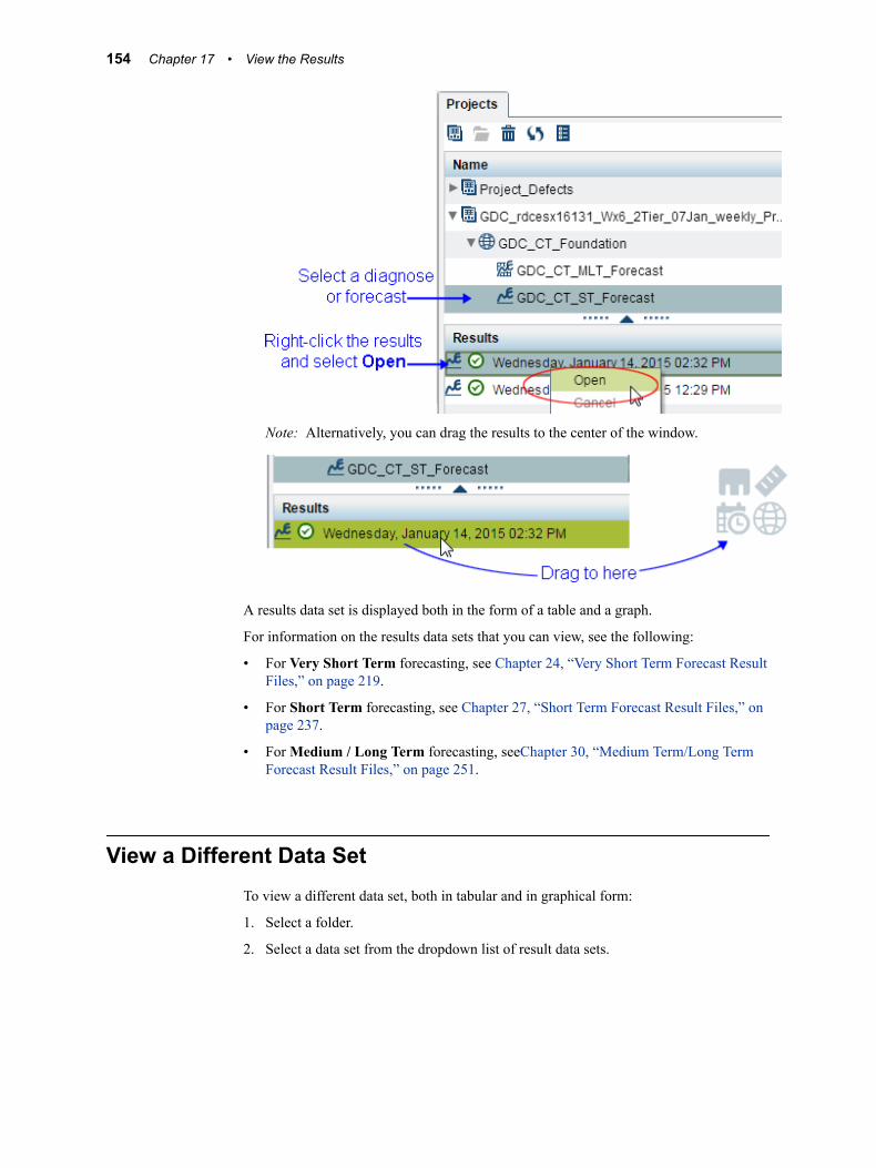
Note: Alternatively, you can drag the results to the center of the window.

A results data set is displayed both in the form of a table and a graph.

For information on the results data sets that you can view, see the following:

• For Very Short Term forecasting, see Chapter 24, “Very Short Term Forecast Result Files,” on page 219.

• For Short Term forecasting, see Chapter 27, “Short Term Forecast Result Files,” on page 237.

• For Medium / Long Term forecasting, seeChapter 30, “Medium Term/Long Term Forecast Result Files,” on page 251.

View a Different Data SetTo view a different data set, both in tabular and in graphical form:

1. Select a folder.

2. Select a data set from the dropdown list of result data sets.


3. To select a data set from a different folder, click Change Folder and then select the data set. You can select a data set from the following folders:

• results

• sources

• work

For information on the results data sets that you can view, see the following:

• For Very Short Term forecasting, see Chapter 24, “Very Short Term Forecast Result Files,” on page 219.

• For Short Term forecasting, see Chapter 27, “Short Term Forecast Result Files,” on page 237.

• For Medium / Long Term forecasting, seeChapter 30, “Medium Term/Long Term Forecast Result Files,” on page 251.

View an Additional Graph or TableTo view an additional table or graph:

1. Click the plus sign next to the currently-displayed table.

2. Select Graph or Table.

The Select Graph or Select Table window opens.

View an Additional Graph or Table 155

3. Select the file for which you want to see a graph or table.

The additional graph or table is displayed in a new tab.

Modify the View by Customizing the Query

How To Invoke the Query Specification WindowUse the Query Specification window to specify a custom query whose results are displayed as a graph and table.

To invoke the Query Specification window, click the Query icon at the top left of an open graph.


Specify the QuerySpecify the following parameters to form a custom query whose results are displayed as a graph and table.

Page SizeSpecify how much data is to be read from the database at a time.

Note: Specifying too large a page size can result in the system timing out. If the system becomes unresponsive during a query, you can use the Escape key to cancel the current query and try reducing the page size.

Date FilterSpecify the beginning and end date of the results to be displayed.

Note: Specify None to not filter by date.

Group BySpecify the variable for the X axis.

One point is displayed on the X axis for each distinct value of this variable. For example, if you specify year as the Group By variable, then one point is displayed on the X axis for each calendar year even if there are multiple rows in the database table for the same year. For example, there might be database rows for every day in a year, but only one point would be displayed on the X axis if you group by year.

Column NameSpecify one or more variables for the Y axis.

Because, with the Group By variable, every point on the X axis corresponds to multiple rows in the database, you must specify how to aggregate these rows to display a single point on the Y axis. You can specify SUM, AVG, MIN, MAX.

Modify the View by Customizing the Query 157

ExampleThe picture below shows the graph that results from having selected Date/Time for the X axis and actual_load for the Y axis. You can see that because Date/Time includes an enormous number of rows (one for every point in time at which a load value is obtained), the X axis is crowded with so much data that not all of it fits in the window—you can see that the scroll button is enabled to scroll forward.

To alleviate the situation of an enormous amount of data being displayed on a single graph, the following picture shows a customer query whereby:

Page SizeThe value of Page Size is not changed from the default value. You can experiment with page size, but be careful about asking the system to query more data than your hardware can handle.

Group ByYear is chosen for the X axis instead of Date/Time. The result of choosing year is that instead of displaying one point on the X axis for every point in time at which a load value is obtained, only one point is displayed on the X axis for every year. That is, all the rows for a single year are grouped together and displayed on the graph as a single point.

Column NameBecause, with the Group By variable, every point on the X axis corresponds to multiple rows in the database, you must specify how to aggregate these rows so as to display a single point on the Y axis. In this example AVG is chosen. That is, for each year on the X axis, the average load is displayed for all the Date/Time load observations taken during that year.


The following picture shows the results of the custom query. You can see that instead of one point on the X axis for every Date/Time load observation, there is only one point on the X axis per year. For each year, the average load during that year is displayed on the Y axis. And, you can see that because the number of years represented in the database is able to be displayed in a single graph, the scroll button is disabled.

You can also see that in place of the values chosen for the initial display, the values chosen for the custom query are now displayed under Graph Properties, namely:

X Axis: year

Y Axis: AVG_actual_load

Modify the View by Customizing the Query 159

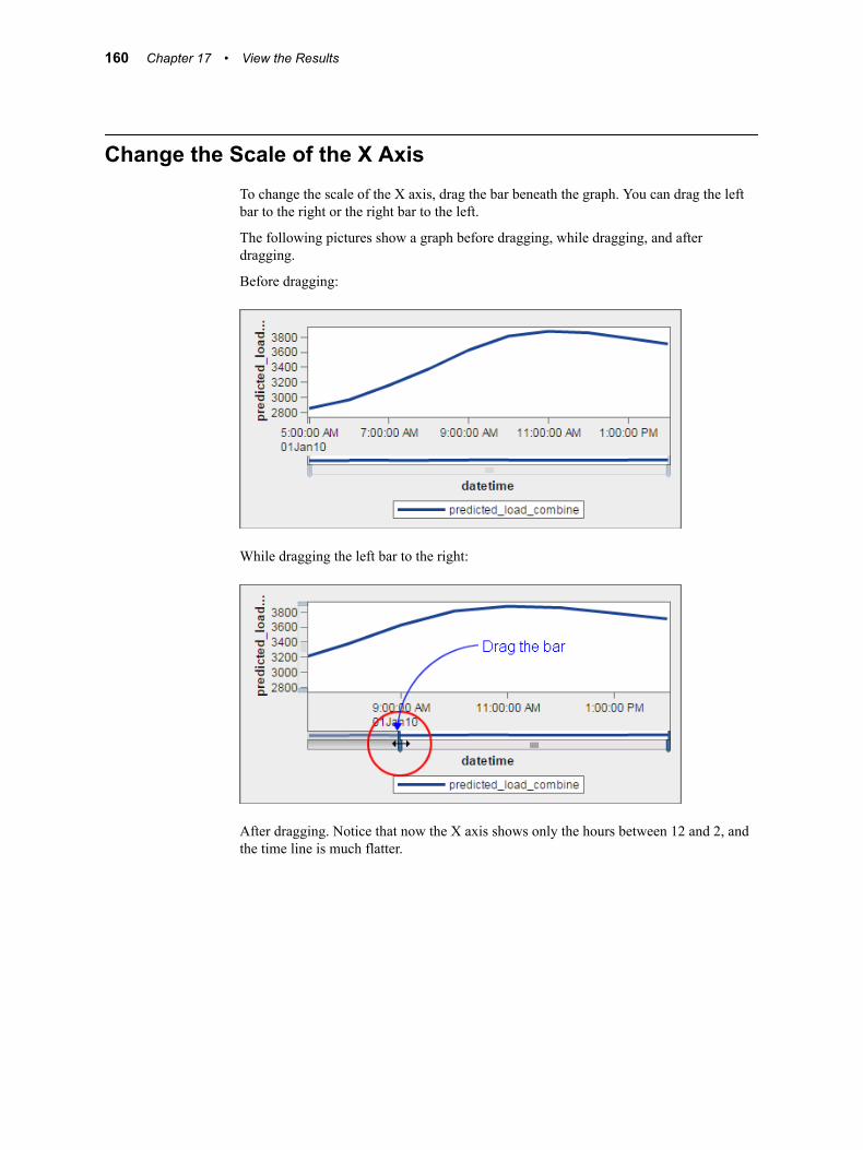
Change the Scale of the X AxisTo change the scale of the X axis, drag the bar beneath the graph. You can drag the left bar to the right or the right bar to the left.

The following pictures show a graph before dragging, while dragging, and after dragging.

Before dragging:

While dragging the left bar to the right:

After dragging. Notice that now the X axis shows only the hours between 12 and 2, and the time line is much flatter.


Filter the ResultsTo filter the result of a query:

1. Select the Additional search options button.

A dialog opens showing all the fields that you can filter on.

2. For each field that you want to filter on, select the values to include in the results.

For example, the following picture shows choosing the values from 6,800 to 7,367 for the field actual_peak and choosing the values 2010 to 2013 for the field Year. Consequently, the graph will show query results that include only the years 2010 to 2013 and only peak values within the specified range.

Filter the Results 161

Note: Filtering applies to an entirely new query. It does not apply to the graph or table already displayed. Therefore, you can select fields to filter on that are not displayed in either the X or the Y axis.







Add CommentsTo add comments to the output of a diagnose or forecast:

1. View the results of a diagnose or forecast. See “View a Table or Graph” on page 153.

2. Click the Comments tab.

3. Type a topic title and topic text.

You can respond to a previous comment by typing in the field labelled Respond to topic.

Add Comments 163

Note: In order to delete a comment, the user must have the SAS Application Infrastructure Delete comments capability. A user has this capability by being a member of a group that has a role with this capability.


Chapter 18

Set User Preferences

Preferences . . . . . . . . . . . . . . . . . . . . . . . . . . . . . . . . . . . . . . . . . . . . . . . . . . . . . . . . . 165

PreferencesYou can set the following user preferences:

• Global Preferences that apply to one user’s use of any SAS Web application

• SAS Energy Forecasting preferences that apply to one user’s use of SAS Energy Forecasting.

To set SAS Energy Forecasting user preferences:

1. Select File ð Preferences.

2. Select SAS Energy Forecasting.

3. Select among the following preferences:

Show System ParametersSelect this option to show the System tab on windows where you set or edit forecast and diagnose parameters. Deselect this option to hide the tab.

Because you do not often change system parameters, you might want to hide them to prevent their being changed inadvertently.

Filter Archived InstancesWhen you archive diagnose and forecast results, they are moved to an archive location and deleted from their original location. However, they can continue to show up in the list of more recent diagnose and forecast results.

Note: You cannot open archived results with the SAS Energy Forecasting user interface. You must open them from their archived location.

• Select Filter Archived Instances so as not to show archived results along with more recent results.

• Deselect Filter Archived Instances so as to show archived results along with more recent results.

For information about archiving, see Chapter 9, “Archive Results Data,” on page 71.

165

Filter Results After # WeeksSpecify a number of weeks so as not to show diagnose and forecast results that are older than the number of weeks specified. For example, if you specify 5 weeks, then diagnose and forecast results that are more than 5 weeks old are not listed along with more recent diagnose and forecast results.

166 Chapter 18 • Set User Preferences

Part 4

Foundation Diagnose

Chapter 19Parameters for a Foundation Diagnose . . . . . . . . . . . . . . . . . . . . . . . . . . 169

Chapter 20The Diagnose Process . . . . . . . . . . . . . . . . . . . . . . . . . . . . . . . . . . . . . . . . . . 185

Chapter 21Diagnose Result Files . . . . . . . . . . . . . . . . . . . . . . . . . . . . . . . . . . . . . . . . . . 191

167

Chapter 19

Parameters for a Foundation Diagnose

Main Parameters: Weights . . . . . . . . . . . . . . . . . . . . . . . . . . . . . . . . . . . . . . . . . . . . 170Weight . . . . . . . . . . . . . . . . . . . . . . . . . . . . . . . . . . . . . . . . . . . . . . . . . . . . . . . . . . . 170Weight Lower . . . . . . . . . . . . . . . . . . . . . . . . . . . . . . . . . . . . . . . . . . . . . . . . . . . . . 170Weight Upper . . . . . . . . . . . . . . . . . . . . . . . . . . . . . . . . . . . . . . . . . . . . . . . . . . . . . 170

Main Parameters: Periods . . . . . . . . . . . . . . . . . . . . . . . . . . . . . . . . . . . . . . . . . . . . . 171Training Start Date . . . . . . . . . . . . . . . . . . . . . . . . . . . . . . . . . . . . . . . . . . . . . . . . . 171Rolling Start Date . . . . . . . . . . . . . . . . . . . . . . . . . . . . . . . . . . . . . . . . . . . . . . . . . . 171Rolling End Date . . . . . . . . . . . . . . . . . . . . . . . . . . . . . . . . . . . . . . . . . . . . . . . . . . 171Sub Hour . . . . . . . . . . . . . . . . . . . . . . . . . . . . . . . . . . . . . . . . . . . . . . . . . . . . . . . . . 172Sub Date Offset . . . . . . . . . . . . . . . . . . . . . . . . . . . . . . . . . . . . . . . . . . . . . . . . . . . . 172

MAPE Parameters: Type . . . . . . . . . . . . . . . . . . . . . . . . . . . . . . . . . . . . . . . . . . . . . . 172MAPE . . . . . . . . . . . . . . . . . . . . . . . . . . . . . . . . . . . . . . . . . . . . . . . . . . . . . . . . . . . 172

MAPE Parameters: Weights . . . . . . . . . . . . . . . . . . . . . . . . . . . . . . . . . . . . . . . . . . . 174Weight Hourly MAPE . . . . . . . . . . . . . . . . . . . . . . . . . . . . . . . . . . . . . . . . . . . . . . 174Weight Daily MAPE . . . . . . . . . . . . . . . . . . . . . . . . . . . . . . . . . . . . . . . . . . . . . . . . 174Weight Daily Peak MAPE . . . . . . . . . . . . . . . . . . . . . . . . . . . . . . . . . . . . . . . . . . . 174Weight Monthly MAPE . . . . . . . . . . . . . . . . . . . . . . . . . . . . . . . . . . . . . . . . . . . . . 175Weight Monthly Peak MAPE . . . . . . . . . . . . . . . . . . . . . . . . . . . . . . . . . . . . . . . . . 175Weight Annual MAPE . . . . . . . . . . . . . . . . . . . . . . . . . . . . . . . . . . . . . . . . . . . . . . 175Weight Annual Peak MAPE . . . . . . . . . . . . . . . . . . . . . . . . . . . . . . . . . . . . . . . . . . 175MAPE Improvement . . . . . . . . . . . . . . . . . . . . . . . . . . . . . . . . . . . . . . . . . . . . . . . . 176

Advanced Parameters . . . . . . . . . . . . . . . . . . . . . . . . . . . . . . . . . . . . . . . . . . . . . . . . 176Outlier Percent . . . . . . . . . . . . . . . . . . . . . . . . . . . . . . . . . . . . . . . . . . . . . . . . . . . . 176Residual History Length . . . . . . . . . . . . . . . . . . . . . . . . . . . . . . . . . . . . . . . . . . . . . 176Combine Forecast . . . . . . . . . . . . . . . . . . . . . . . . . . . . . . . . . . . . . . . . . . . . . . . . . . 177Poly Order . . . . . . . . . . . . . . . . . . . . . . . . . . . . . . . . . . . . . . . . . . . . . . . . . . . . . . . . 177APE Cutoff . . . . . . . . . . . . . . . . . . . . . . . . . . . . . . . . . . . . . . . . . . . . . . . . . . . . . . . 177Two Stage . . . . . . . . . . . . . . . . . . . . . . . . . . . . . . . . . . . . . . . . . . . . . . . . . . . . . . . . 177Default Weather Type Code . . . . . . . . . . . . . . . . . . . . . . . . . . . . . . . . . . . . . . . . . . 178WLS . . . . . . . . . . . . . . . . . . . . . . . . . . . . . . . . . . . . . . . . . . . . . . . . . . . . . . . . . . . . 178Additional Modeling Variables . . . . . . . . . . . . . . . . . . . . . . . . . . . . . . . . . . . . . . . . 178Additional Class Variables . . . . . . . . . . . . . . . . . . . . . . . . . . . . . . . . . . . . . . . . . . . 178

System Parameters . . . . . . . . . . . . . . . . . . . . . . . . . . . . . . . . . . . . . . . . . . . . . . . . . . . 179Number of CPUs . . . . . . . . . . . . . . . . . . . . . . . . . . . . . . . . . . . . . . . . . . . . . . . . . . . 179Input Path . . . . . . . . . . . . . . . . . . . . . . . . . . . . . . . . . . . . . . . . . . . . . . . . . . . . . . . . 179Data Model . . . . . . . . . . . . . . . . . . . . . . . . . . . . . . . . . . . . . . . . . . . . . . . . . . . . . . . 179Fixed Date Holidays . . . . . . . . . . . . . . . . . . . . . . . . . . . . . . . . . . . . . . . . . . . . . . . . 179Diagnose Initialization Exit . . . . . . . . . . . . . . . . . . . . . . . . . . . . . . . . . . . . . . . . . . 180Diagnose Completion Exit . . . . . . . . . . . . . . . . . . . . . . . . . . . . . . . . . . . . . . . . . . . 180

169

Parameter Selection and Forecast Performance . . . . . . . . . . . . . . . . . . . . . . . . . . . 180Overview . . . . . . . . . . . . . . . . . . . . . . . . . . . . . . . . . . . . . . . . . . . . . . . . . . . . . . . . . 180Very Short Term Load Forecasts . . . . . . . . . . . . . . . . . . . . . . . . . . . . . . . . . . . . . . 181Short Term Forecasts . . . . . . . . . . . . . . . . . . . . . . . . . . . . . . . . . . . . . . . . . . . . . . . 183Medium Term/Long Term Forecasts . . . . . . . . . . . . . . . . . . . . . . . . . . . . . . . . . . . 183

Main Parameters: Weights

WeightEnter the number of weights utilized to calculate the weighted average temperature. The calculation is exponentially smoothed.

You can choose up to four different models for calculating the weighted average temperature based on up to four corresponding weights. Valid values: 1, 2, 3, or 4. If you set Weight=1, then, Weight Lower should equal Weight Upper. Default is 4.

Applies to the Recency model.

Column name in table: weight_num

Weight LowerEnter the lower boundary of the weight utilized to calculate the exponentially smoothed temperature. Valid values are between 0.8 and 1. Default is 0.8.


Column name in table: weight_lower

Weight UpperEnter the upper boundary of the weight utilized to calculate the exponentially smoothed temperature. Valid values are between 0.8 and 1. Default is 0.95.

Note: If the number of weights is 1, then Weight Lower should equal Weight Upper.


Column name in table: weight_upper

170 Chapter 19 • Parameters for a Foundation Diagnose

Main Parameters: Periods

Training Start DateSelect the start date of the historical data to be used to “train” the diagnose model so that it selects the best model. Set the start date of training data to be equal to or later than the start date of the utility’s historical load data (the total input of historical data that is available).

You should have at least two years of data for model training to produce a good diagnose and three years is better.

Column name in table: train_start_date

Rolling Start DateSelect the start date of the holdout period. The holdout period is the period between the Rolling Start Date and the Rolling End Date. By comparing the forecast results of a particular model with the actual load data in the holdout period (which data is not used in creating the diagnose model), the system calculates a MAPE that is used to select the best model.

The Rolling Start Date should be at least 12 months later than the Training Start Date. The training period extends from the Training Start Date up to the Rolling Start Date.

Note: How you specify the holdout period can affect how long it takes to do a very short term load forecast. See “Parameter Selection and Forecast Performance” on page 180.

Column name in table: rolling_start_date

Rolling End DateSelect the end date of the holdout period. The holdout period is the period between the Rolling Start Date and the Rolling End Date. Following are suggested lengths for the holdout period:

• Very Short Term: Last 7 days. For more information, see “Parameter Selection and Forecast Performance” on page 180.

• Short Term: Last 30 days

Main Parameters: Periods 171

• Medium Term/Long Term: Minimum 1 year, and 2–3 years preferred

Note: How you specify the holdout period can affect how long it takes to do a very short term load forecast. See “Parameter Selection and Forecast Performance” on page 180.

Column name in table: rolling_end_date

Sub HourEnter the hour for submission (usually 7). For example, 7 means 7 AM.

Column name in table: sub_hour

Sub Date OffsetEnter the number of days (usually 1) between the date of submission and the date of forecast.

Column name in table: sub_date_offset

MAPE Parameters: Type

MAPEEnter the criterion for selecting the best (“champion”) model.

Note:

• ME = Mean error

• MAE = Mean absolute error

• MAPE = Mean absolute percentage error

The MAPE selected provides the criteron used for selecting the best (champion) model. It is calculated by comparing the forecast results of a model with the actual load data in the holdout period (the period between the Rolling Start Date and the Rolling End Date). The load data in the holdout period is not used in creating the diagnose model.

The value can be any of the following:

• hourly_me

• hourly_mae


• hourly_mape

• daily_me

• daily_mae

• daily_mape

• daily_peak_me

• daily_peak_mae

• daily_peak_mape

• monthly_me

• monthly_mae

• monthly_mape

• monthly_peak_me

• monthly_peak_mae

• monthly_peak_mape

• annual_me

• annual_mae

• annual_mape

• annual_peak_me

• annual_peak_mae

• annual_peak_mape

• weighted_mape

Column name in table: mape

See Also“Error Analysis Equations” on page 189

MAPE Parameters: Type 173

MAPE Parameters: WeightsWeight parameters apply only if you selected weight_mape as the type of MAPE to use for choosing the best model.

Weight Hourly MAPEWeighted Hourly Mean Absolute Percentage Error

This is the weight assigned to hourly MAPE in calculating weighted_mape. The weight must be less than or equal to 1 and the sum of all weights must equal to 1. Enter a decimal value rather than a percentage value. For example, 0.1 rather than 10%.

Column name in table: w_hourly_mape

Note: This parameter applies only if you selected weighted_mape as the type of MAPE to use in choosing the best model.

Weight Daily MAPEWeighted Daily Mean Absolute Percentage Error

This is the weight assigned to daily energy MAPE in calculating weighted_mape. The weight must be less than or equal to 1 and the sum of all weights must equal to 1. Enter a decimal value rather than a percentage value. For example, 0.1 rather than 10%.

Column name in table: w_daily_mape


Weight Daily Peak MAPEWeighted Daily Peak Mean Absolute Percentage Error


This is the weight assigned to daily peak MAPE in calculating weighted_mape. The weight must be less than or equal to 1 and the sum of all weights must equal to 1. Enter a decimal value rather than a percentage value. For example, 0.1 rather than 10%.

Column name in table: w_daily_peak_mape


Weight Monthly MAPEWeighted Monthly Mean Absolute Percentage Error

This is the weight assigned to monthly energy MAPE in calculating weighted_mape. The weight must be less than or equal to 1 and the sum of all weights must equal to 1. Enter a decimal value rather than a percentage value. For example, 0.1 rather than 10%.

Column name in table: w_monthly_mape


Weight Monthly Peak MAPEWeighted Monthly Peak Mean Absolute Percentage Error

This is the weight assigned to monthly peak MAPE in calculating weighted_mape. The weight must be less than or equal to 1 and the sum of all weights must equal to 1. Enter a decimal value rather than a percentage value. For example, 0.1 rather than 10%.

Column name in table: w_monthly_peak_mape


Weight Annual MAPEWeighted Annual Mean Absolute Percentage Error

This is the weight assigned to annual energy MAPE in calculating weighted_mape. The weight must be less than or equal to 1 and the sum of all weights must equal to 1. Enter a decimal value rather than a percentage value. For example, 0.1 rather than 10%.

Column name in table: w_annual_mape


Weight Annual Peak MAPEWeighted Annual Peak Mean Absolute Percentage Error

This is the weight assigned to annual peak MAPE in calculating weighted_mape. The weight must be less than or equal to 1 and the sum of all weights must equal to 1. Enter a decimal value rather than a percentage value. For example, 0.1 rather than 10%.

Column name in table: w_annual_peak_mape

MAPE Parameters: Weights 175


MAPE ImprovementOnly if the model MAPE improvement is higher than the entered value should the forecasting improvement be considered significant. The default value is 0.0001.

Column name in table: mape_improvement


Advanced Parameters

Outlier PercentEnter the percentage of observations that are to be considered as outliers. The default value is 0.001 which means the generated outlier table includes the top 0.1 percent of all observations with the largest forecast absolute error (AE).

Note: Enter the number as a decimal value rather than as a percentage. For example, enter 0.001 rather than 0.1%.

The value that you specify for APE Cutoff then determines which of the outliers are chosen.

Column name in table: outlier_percent

Residual History LengthChoose the length of time during which to calculate the residual used in the two-stage model (integer value with unit of hour).The default value is 504, which means utilizing


the residual of the previous 504 hours (21 days; three weeks). The residual is the difference between the forecast value and the actual value.

Note: Choosing too short a residual history length can have the result that values don’t converge. A length of around 500 hours should be adequate.

Column name in table: residual_hist_length

Combine ForecastThis parameter controls which two-stage model(s) will be included for calculating the combined forecast. The value for this parameter will be various combinations of 1, 2, 3 and 4.

1=GLM_ARIMA (auto regressive integrated moving average)

2=GLM_ESM (exponential smoothing modeling)

3=GLM_UCM (unobserved components modeling)

4=GLM_NN (neural network)

For example, 1234 means use GLM_ARIMA, GLM_ESM, GLM_UCM and GLM_NN to calculate the combined forecast, and 124 means use GLM_ARIMA, GLM_ESM and GLM_NN to calculate the combined forecast.

The default value is 1234 and the combined forecast will be calculated only if the two_stage models are enabled and the best model from the diagnose procedure is a combined forecast

Colomn name in table: combine_fcst

Poly OrderControl using 2nd or 3rd order polynomial of the temperature variables in the model. The value of this parameter should be either 2 or 3. Specifying 3 does result in it taking longer to do the diagnose.

Column name in table: poly_order

APE CutoffThe APE Cutoff determines which observations are put into the outlier table. Observations with absolute percentage error greater than this threshold will be put into the table.

Note: Enter the number as a decimal value rather than as a percentage. For example, enter 0.05 rather than 5%.

The value that you enter for Outlier Percent determines the percentage of observations that are considered as outliers.

Column name in table: ape_cutoff

Two StageEnter YES to run the two-stage model.

Enter NO to run the one-stage model.

Note:

Advanced Parameters 177

• Choosing one-stage or two-stage can affect how long it takes to do a very short term load forecast. See “Parameter Selection and Forecast Performance” on page 180.

• The two-stage model is not recommended if there is insufficient historical data.

See “Two-Stage Model” on page 188.

Column name in table: two_stage

Default Weather Type CodeSpecifies the type of data contained in the WTHR_NO field of the weather data source file.

Note: This parameter applies only to a weather table in 3.1 data model format. See “Weather Data Table” on page 57.

Valid values are:

TEMPFFahrenheit

TEMPCCentigrade

Column name in table: default_wthr_type_cd

WLSEnter YES if the weighted least squares (WLS) model is desired. Otherwise, enter NO.

Column name in table: wls

Additional Modeling VariablesVariables that you specify in this field are used in the MODEL statement of PROC GLM as independent effects. For more information, see Chapter 8, “Add Additional Variables as Parameters,” on page 67.


Column name in table: add_var

Additional Class VariablesAdd a class variable. Variables that you specify in this field are used in the CLASS statement of PROC GLM as additional class variables. For more information, see Chapter 8, “Add Additional Variables as Parameters,” on page 67.


Column name in table: add_class


System Parameters

Number of CPUsSAS Energy Forecasting can run parallel processing, which significantly reduces processing time. Select the number of available CPU cores to define how many parallel processes should be run.

Column name in table: num_cpu

Input PathSpecifies the folder containing the input files to SAS Energy Forecasting. You can override the system-specified folder if you want your input files are in a different location.

Column name in table: staged_data_path

See also: Chapter 5, “Prepare the Input Files,” on page 47.

Data ModelChoose the format of the source files to be used for forecasting. Valid values are 3.1 and 2 (3.1 being the newer data model).

Column name in table: data_model

Fixed Date HolidaysUsing a numeric code, specify the holidays whose calendar date does not differ from year to year. Separate each numeric code with a blank. The default for the US calendar is 1 5 8 10.

• 1=New Years Day: January 1

• 5=Independence Day: July 4

• 8=Veterans Day: November 11

• 10=Christmas: December 25

System Parameters 179

Codes for the US holidays whose calendar date varies from year to year are the following:

• 2=Martin Luther King’s Birthday

• 3=George Washington’s Birthday

• 4=Memorial Day

• 6=Labor Day

• 7=Columbus Day

• 9=Thanksgiving Day

Column name in table: fix_date_holiday_list

Diagnose Initialization ExitThis parameter is optional.

Specify the path and file name of a SAS program or macro that SAS Energy Forecasting will invoke before the diagnose is run. For example: C:\hana\init.sas.

Typically, you can use such a program to allocate resources and make connections that might be needed for the diagnose.

Note: If you specify such a program, then you probably want also to specify a program with Diagnose Completion Exit to free the resources and connections made during initialization.

Column name in table: sefdg_init_exit.xml

Diagnose Completion ExitThis parameter is optional.

Specify the path and file name of a SAS program or macro that SAS Energy Forecasting will invoke after the diagnose is finished. For example: C:\hana\terminate.sas.

Typically, you can use such a program to free resources and connections that you made with your program specified in Diagnose Initialization Exit.

Column name in table: sefdg_term_exit.xml

Parameter Selection and Forecast Performance

OverviewIt is recommended that you have a different diagnose for each type of forecast: short term, very short term, and medium/long term. How you specify parameters for a diagnose affects both how long it takes to run a forecast and the forecast MAPE. Generally a diagnose can take from one hour to as long as 8 hours to run, so it is recommended that that you run these at night or over the weekend. SAS Energy Forecasting has an adjustable timer that is defaulted to allow a solution to run up to 12 hours before it times out. If a diagnose fails due to this default, you can adjust the value by changing the System time out, in minutes ... setting. See “Application Settings” on page 65.


If during the setup for a forecast run, you decide to output report data to the server, the execution times will probably increase due to the large volumes of data being appended to the report files. See Chapter 11, “Produce Reports,” on page 83.

Very Short Term Load Forecasts

Run TimeThe amount of time required to run a forecast depends primarily on your choice of the following parameters:

• One or Two Stage model

• Holdout period (Rolling End Date – Rolling Start Date)

• Training period

• History length

One or Two Stage

The choice of either one or two stage model in diagnose will determine how many models are consumed in the diagnose and subsequently the forecast process. Generally a one stage model in diagnose will result in two models being consumed in the forecast. If a two stage model is selected in diagnose, typically up to 7 models are consumed in the forecast. The more models being consumed in the forecast the longer the execution time.

Selecting a two stage model as the diagnose parameter does not guarantee that a two stage model will be chosen as the champion model. The length of the holdout or rolling period selected in diagnose also has an impact on the champion model chosen during the diagnose process.

See Chapter 20, “The Diagnose Process,” on page 185.

Holdout period

The holdout period is the period between Rolling Start Date and Rolling End Date. The holdout period is a selected subset of the historical data that is held from the data used in developing the various models but is used later to test the accuracy of the various models during error analysis process by calculating mean error (ME), mean absolute error (MAR), and mean absolute percentage error (MAPE). A shorter rolling or holdout period typically results in the diagnose process selecting a single stage model as the best or champion model. A longer rolling period typically results in the diagnose process

Parameter Selection and Forecast Performance 181

selecting a two stage model as the best or champion model. When a forecast is run against the diagnose, the number of models used in the analysis depends on whether a one stage or two stage model was selected as the champion model. A one stage model typically uses 2 models in the forecast while a two stage model can have up to 7 models being consumed during the forecast process. And, the more models used the longer it takes to do the forecast. Basic rules of thumb are:

• Longer holdout results in the best model from a diagnose being a two-stage model.

• Shorter holdout results in the best model from a diagnose being a one-stage model. In general, a one-stage model for diagnose results in a faster forecast than a two-stage diagnose.

Training Period and History LengthThe training period extends from the Training Start Date up to the Rolling Start Date.The longer the training period selected during the diagnose process and the longer the history length selected during the forecast process, more data is used in the calculations and therefore a longer execution time can be expected. Generally the more historical load data that is consumed in the diagnose and forecast processes, the more improvement in accuracy of the model can be expected, as measured by hourly MAPE.

MAPEThe forecast MAPE also depends primarily on your choice of the same parameters:

One or Two StageGenerally a two-stage model for diagnose results in a better MAPE for the resulting forecast.

Holdout Period (Rolling End Date – Rolling Start Date)In general, the longer the holdout period for diagnose, the better the MAPE for the resulting forecast.

Trade Off Between Run Time and MAPEWhen performing very short term forecasting analysis, there is a trade off that must be made between forecast run time and forecast accuracy or MAPE. Extensive testing has provided the following results:

• A longer rolling or holdout period generally results in a two stage model being chosen as the champion model which in turn results in the forecast consuming more models in the analysis. More models translates into a longer run time.

• A longer training period chosen in diagnose and a long history length selected in forecast generally result in longer run times because of the volume of data consumed in the analysis.


• The more data consumed in the forecast process, the better accuracy or MAPE that can be expected. The trade off is in run time.

• Tests have produced run times in excess of 20 minutes when performing very short term forecasts looking 24 hours or longer into the future. Forecasters generally perform very short term forecasting on an hourly schedule which dictates that run times should be held to a minimum, typically 5 minutes or less.

Short Term ForecastsShort term forecasts are typically run monthly or quarterly, so execution times are not as important as in very short term forecasts. • A holdout period of 30 to 90 days with 2-stage diagnose is sufficient to produce acceptable MAPEs in short term forecasts. Testing has produced run times that are generally less than 5 minutes. Longer rolling periods and more history data generally produce better accuracy as measured by hourly MAPE.

Medium Term/Long Term ForecastsMedium term/Long term forecasts are typically run once or twice a year, so execution times are not critical.

• A holdout period of 90 days or more with 2-stage diagnose will produce acceptable MAPEs in medium term/long term forecasts.

• A longer holdout period results in longer execution times, so a medium term/long term diagnose can be run at night or on weekends.

Parameter Selection and Forecast Performance 183

Chapter 20

The Diagnose Process

One-Stage Model . . . . . . . . . . . . . . . . . . . . . . . . . . . . . . . . . . . . . . . . . . . . . . . . . . . . . 185Overview . . . . . . . . . . . . . . . . . . . . . . . . . . . . . . . . . . . . . . . . . . . . . . . . . . . . . . . . . 185Step 1: Generate a Naive Model . . . . . . . . . . . . . . . . . . . . . . . . . . . . . . . . . . . . . . . 186Step 2: Add the Recency Effect . . . . . . . . . . . . . . . . . . . . . . . . . . . . . . . . . . . . . . . 186Step 3: Add the Calendar (Weekend) Effect . . . . . . . . . . . . . . . . . . . . . . . . . . . . . . 187Step 4: Add the Holiday Effect . . . . . . . . . . . . . . . . . . . . . . . . . . . . . . . . . . . . . . . . 187Step 5: Calculate Weighted Least Squares (WLS) . . . . . . . . . . . . . . . . . . . . . . . . . 187Step 6: Analyze Errors . . . . . . . . . . . . . . . . . . . . . . . . . . . . . . . . . . . . . . . . . . . . . . 188Step 7: Detect Outliers . . . . . . . . . . . . . . . . . . . . . . . . . . . . . . . . . . . . . . . . . . . . . . 188

Two-Stage Model . . . . . . . . . . . . . . . . . . . . . . . . . . . . . . . . . . . . . . . . . . . . . . . . . . . . 188

Error Analysis Equations . . . . . . . . . . . . . . . . . . . . . . . . . . . . . . . . . . . . . . . . . . . . . . 189

One-Stage Model

OverviewThe diagnose uses the training period data as specified in the diagnose parameters to step though a sequence of possible models. The models are tested against the holdout period defined in the diagnose parameters to determine the best models according to the error definition. Diagnose is a prerequisite process that must be run before any forecasts are developed. The following diagram depicts the diagnose process which is explained in more detail in the subsequent text.

185

Step 1: Generate a Naive ModelAs the first step, a naïve benchmark model is generated. This is described by the following equation known as GLMLF-B:

By comparing the forecast results of a particular model with the actual load data in the holdout period (which data is not used in the forecast), the system calculates a MAPE that is used to select the best model.

Step 2: Add the Recency EffectAs the second step, the recency effect is added using models that include combinations of the following:

• the simple moving average of the temperatures from the preceding 24 hours

• temperatures from preceding hours

• weighted moving average of the temperatures from the preceding 24 hours

186 Chapter 20 • The Diagnose Process

The forecast for each model combination is tested in the holdout period based on the MAPE or APE specified by the user in the diagnose parameters. After this comparison, the winning model proceeds to the next step.

Step 3: Add the Calendar (Weekend) EffectThe weekend effect is added to the winning model from the recency effect. This is done by grouping two adjacent days together and calculating the holdout MAPE generated by this grouping method. Only if the holdout MAPE improves should those two days continue to be grouped. All adjacent days are tried: Monday/ Tuesday, Tuesday/Wednesday, Wednesday/Thursday, Thursday/Friday, Friday/Saturday, Saturday/Sunday, and Sunday/Monday.

Step 4: Add the Holiday EffectThe holiday effect is added into the winning model from the weekend effect. Holidays are defined in the Calendar table to reflect the local situation. See “Calendar Table” on page 47. The following structure is used to define an unlimited number of holidays. The structure allows the day prior and following to be defined as special days where variations from normal load occur.

special_day Holiday

1 New Year’s Day

101 New Year’s Eve

201 Day after New Year’s Day

2 Martin Luther King, Jr.’s Birthday

102 Day before Martin Luther King, Jr.’s Birthday

202 Day after Martin Luther King, Jr.’s Birthday

Models are first developed with the special days modeled as the weekday on which they occur. Models are then developed to test the special day considered to be all other day types of the week. If considering a special day as another day of the week improves model accuracy, then its weekday assignment is modified.

Step 5: Calculate Weighted Least Squares (WLS)The winning model from the holiday model is modified to include four different exponential weighted least square weighted temperature combinations. To emphasize recent status, higher weights are assigned to more recent observations, and an exponential WLS approach can be deployed. The winning model from the four candidates is chosen.

One-Stage Model 187

Step 6: Analyze ErrorsThe winning model in each step is tested against the holdout period. The following error statistics are calculated for each of the models to identify the best model to use for forecasting:

• Hourly load (ME, MAE, and MAPE)

• Daily peak load (ME, MAE, and MAPE)

• Daily energy (ME, MAE, and MAPE)

• Monthly peak load (ME, MAE, and MAPE)

• Monthly energy (ME, MAE, and MAPE)

• Annual peak load (ME, MAE, and MAPE)

• Annual energy (ME, MAE, and MAPE)

Step 7: Detect OutliersFor each model, the hours with the highest error statistics are identified. This allows identification of data errors and model specification problems by reviewing error statistics, load, predicted load, and temperature for each of those hours.

The data in the following sample outlier table is ranked by descending AE and the top n percent (default is 0.1 percent) of the observations are included:

Two-Stage ModelThe procedure for the two-stage diagnose model is as follows:

1. The residual of the best model from the one-stage diagnose process is calculated.

2. The residual is forecasted using:

• UCM (unobserved components modeling)

• neural network modeling

• ESM (exponential smoothing modeling)

• ARIMAX (auto regressive integrated moving average with exogenous input) modeling

3. The forecasted residual is added back to the forecast load to generate the two-stage forecast load.


4. The best model is chosen by comparing the model performance of all one-stage and two-stage models.

Error Analysis EquationsEquations utilized in the error analysis process are the following

Error

AE

MAE

APE

MAPE

Symmetric mean absolute percentage error (SMAPE)

Square error

Mean squared error (MSE)

Root mean squared error (RMSE)

Error Analysis Equations 189

R-square

Adjusted R-square (ADJRSQ)

Sum of squared errors (SSE)

Schwarz’s Bayesian criterion (SBC)

Akaike information criterion (AIC)


Chapter 21

Diagnose Result Files

FCST_RESULTS . . . . . . . . . . . . . . . . . . . . . . . . . . . . . . . . . . . . . . . . . . . . . . . . . . . . 191

FCST_RESULTS_ALL . . . . . . . . . . . . . . . . . . . . . . . . . . . . . . . . . . . . . . . . . . . . . . . 192

FCST_STAT . . . . . . . . . . . . . . . . . . . . . . . . . . . . . . . . . . . . . . . . . . . . . . . . . . . . . . . . 193

HOLIDAY_LKP_CT . . . . . . . . . . . . . . . . . . . . . . . . . . . . . . . . . . . . . . . . . . . . . . . . . 194

OUTLIER_TABLE_GLMLFB . . . . . . . . . . . . . . . . . . . . . . . . . . . . . . . . . . . . . . . . . 195

OUTLIER_TABLE_HOLIDAY . . . . . . . . . . . . . . . . . . . . . . . . . . . . . . . . . . . . . . . . 195

OUTLIER_TABLE_NAIVE . . . . . . . . . . . . . . . . . . . . . . . . . . . . . . . . . . . . . . . . . . . 196

OUTLIER_TABLE_RECENCY . . . . . . . . . . . . . . . . . . . . . . . . . . . . . . . . . . . . . . . . 197

OUTLIER_TABLE_RT0 . . . . . . . . . . . . . . . . . . . . . . . . . . . . . . . . . . . . . . . . . . . . . . 197

OUTLIER_TABLE_RT1 . . . . . . . . . . . . . . . . . . . . . . . . . . . . . . . . . . . . . . . . . . . . . . 198

OUTLIER_TABLE_RT2 . . . . . . . . . . . . . . . . . . . . . . . . . . . . . . . . . . . . . . . . . . . . . . 199

OUTLIER_TABLE_RT3 . . . . . . . . . . . . . . . . . . . . . . . . . . . . . . . . . . . . . . . . . . . . . . 200

OUTLIER_TABLE_RT4 . . . . . . . . . . . . . . . . . . . . . . . . . . . . . . . . . . . . . . . . . . . . . . 200

OUTLIER_TABLE_RT5 . . . . . . . . . . . . . . . . . . . . . . . . . . . . . . . . . . . . . . . . . . . . . . 201

OUTLIER_TABLE_RT6 . . . . . . . . . . . . . . . . . . . . . . . . . . . . . . . . . . . . . . . . . . . . . . 202

OUTLIER_TABLE_RT7 . . . . . . . . . . . . . . . . . . . . . . . . . . . . . . . . . . . . . . . . . . . . . . 202

OUTLIER_TABLE_WEEKEND . . . . . . . . . . . . . . . . . . . . . . . . . . . . . . . . . . . . . . . 203

OUTLIER_TABLE_WLS . . . . . . . . . . . . . . . . . . . . . . . . . . . . . . . . . . . . . . . . . . . . . 204

PARAMETER_CONTROL_CT . . . . . . . . . . . . . . . . . . . . . . . . . . . . . . . . . . . . . . . . 204

FCST_RESULTSContains forecast results for the best model

The FCST_RESULTS table contains the following columns:

Column Name Label

date Date

191

Column Name Label

datetime Datetime

he Hour

actual_load Actual Load

predicted_load Predicted Load Combined

FCST_RESULTS_ALLContains forecast results for all models:

• Naïve

• Recency effect

• Weekend effect

• Holiday effect

• WLS (weighted least squares)

• GLM_UCM (unobserved components modeling) if two-stage models are enabled

• GLM_NN (neural network) if two-stage models are enabled

• GLM_ESM (exponential smoothing modeling) if two-stage models are enabled

• GLM_ARIMA (auto regressive integrated moving average) if two-stage models are enabled

• COMBINE if two-stage models are enabled

The FCST_RESULTS_ALL table contains the following columns:

Column Name Label


date Date

datetime Datetime

he Hour

predicted_load_glmlfb Naive Model Predicted Load

predicted_load_glmlfbr Recency Effect Model Predicted Load

predicted_load_glmlfbrw Weekend Effect Model Predicted Load

predicted_load_glmlfbrwh Holiday Effect Model Predicted Load

192 Chapter 21 • Diagnose Result Files

Column Name Label

predicted_load_glmlfwebrwh Holiday Effect WLS (weighted least squares) Model Predicted Load

predicted_load_glm_esm Predicted Load GLM_ESM (exponential smoothing modeling)

predicted_load_glm_arimax Predicted Load GLM_ARIMAX (auto regressive integrated moving average with exogenous input)

predicted_load_glm_ucm Predicted Load GLM_UCM (unobserved components modeling)

predicted_load_glm_nn Predicted Load GLM_NN (neural network)

FCST_STATContains the error matrix for the following models:

• Naïve

• Recency effect

• Weekend effect

• Holiday effect

• WLS (weighted least squares)

• GLM_UCM (unobserved components modeling) if two-stage models are enabled

• GLM_NN (neural network) if two-stage models are enabled

• GLM_ESM (exponential smoothing modeling) if two-stage models are enabled

• GLM_ARIMA (auto regressive integrated moving average) if two-stage models are enabled

• COMBINE if two-stage models are enabled

Statistics include MAE, MAPE, and ME for annual energy, annual peak load, daily energy, daily peak load, monthly energy, monthly peak load, and hourly load.

The FCST_STAT table contains the following columns:

Column Name Label

annual_mae Annual Mean Absolute Error

annual_mape Annual Mean Absolute Percentage Error

annual_me Annual Mean Error

annual_peak_mae Monthly Peak Mean Absolute Error

FCST_STAT 193

Column Name Label

annual_peak_mape Monthly Peak Mean Absolute Percentage Error

annual_peak_me Monthly Peak Mean Error

daily_mae Daily Mean Absolute Error

daily_mape Daily Mean Absolute Percentage Error

daily_me Daily Mean Error

daily_peak_mae Daily Peak Mean Absolute Error

daily_peak_mape Daily Peak Mean Absolute Percentage Error

daily_peak_me Daily Peak Mean Error

hourly_mae Hourly Mean Absolute Error

hourly_mape Hourly Mean Absolute Percentage Error

hourly_me Hourly Mean Error

model_name Model Name

monthly_mae Monthly Mean Absolute Error

monthly_mape Monthly Mean Absolute Percentage Error

monthly_me Monthly Mean Error

monthly_peak_mae Monthly Peak Mean Absolute Error

monthly_peak_mape Monthly Peak Mean Absolute Percentage Error

monthly_peak_me Monthly Peak Mean Error

weighted_mape Weighted Mean Absolute Percentage Error

HOLIDAY_LKP_CTHoliday look-up table used to determine significance of date

The HOLIDAY_LKP_CT table contains the following columns:


Column Name Label

hgroup Holiday Group

special_day Holiday

weekday Weekday

OUTLIER_TABLE_GLMLFBContains percentage of all observations (based on “outlier_percent” parameter) with largest forecast absolute error for naïve model

The OUTLIER_TABLE_GLMLFB table contains the following columns:

Column Name Label

Holiday Holiday Indicator

Weekday Weekday


ae Absolute Error

ape Absolute Percentage Error

datetime Datetime

e Error

outlier_flag Outlier Flag

predicted_load Predicted Load

t0_p1 Temperature

wd_orig Original Weekday

OUTLIER_TABLE_HOLIDAYContains percentage of all observations (based on “outlier_percent” parameter) with largest forecast absolute error for holiday effect model

The OUTLIER_TABLE_HOLIDAY table contains the following columns:

OUTLIER_TABLE_HOLIDAY 195

Column Name Label


Weekday Weekday


ae Absolute Error


datetime Datetime

e Error



t0_p1 Temperature


OUTLIER_TABLE_NAIVEContains percentage of all observations (based on “outlier_percent” parameter) with largest forecast absolute error for naïve model

The OUTLIER_TABLE_NAIVE table contains the following columns:

Column Name Label


Weekday Weekday


ae Absolute Error


datetime Datetime

e Error



Column Name Label


t0_p1 Temperature


OUTLIER_TABLE_RECENCYContains percentage of all observations (based on “outlier_percent” parameter) with largest forecast absolute error for recency effect model

The OUTLIER_TABLE_RECENCY table contains the following columns:

Column Name Label


Weekday Weekday


ae Absolute Error


datetime Datetime

e Error



t0_p1 Temperature


OUTLIER_TABLE_RT0Contains percentage of all observations (based on “outlier_percent” parameter) with largest forecast absolute error for recency effect model step (adding simple moving average of temperature during preceding 24 hours)

The OUTLIER_TABLE_RT0 table contains the following columns:

OUTLIER_TABLE_RT0 197

Column Name Label


Weekday Weekday


ae Absolute Error


datetime Datetime

e Error



t0_p1 Temperature


OUTLIER_TABLE_RT1Contains percentage of all observations (based on “outlier_percent” parameter) with largest forecast absolute error for recency effect model step (adding preceding hour's temperature)


Column Name Label


Weekday Weekday


ae Absolute Error


datetime Datetime

e Error


Column Name Label



t0_p1 Temperature


OUTLIER_TABLE_RT2Contains percentage of all observations (based on “outlier_percent” parameter) with largest forecast absolute error for recency effect model step (changing interaction effects)


Column Name Label


Weekday Weekday


ae Absolute Error


datetime Datetime

e Error



t0_p1 Temperature



OUTLIER_TABLE_RT3Contains percentage of all observations (based on “outlier_percent” parameter) with largest forecast absolute error for recency effect model step (changing more interaction effects)


Column Name Label


Weekday Weekday


ae Absolute Error


datetime Datetime

e Error



t0_p1 Temperature


OUTLIER_TABLE_RT4Contains percentage of all observations (based on “outlier_percent” parameter) with largest forecast absolute error for recency effect model step (replacing average temperature with weighted temperature 1); iterations based on “weight_num” global parameter. See “Weight” on page 170.


Column Name Label


Weekday Weekday


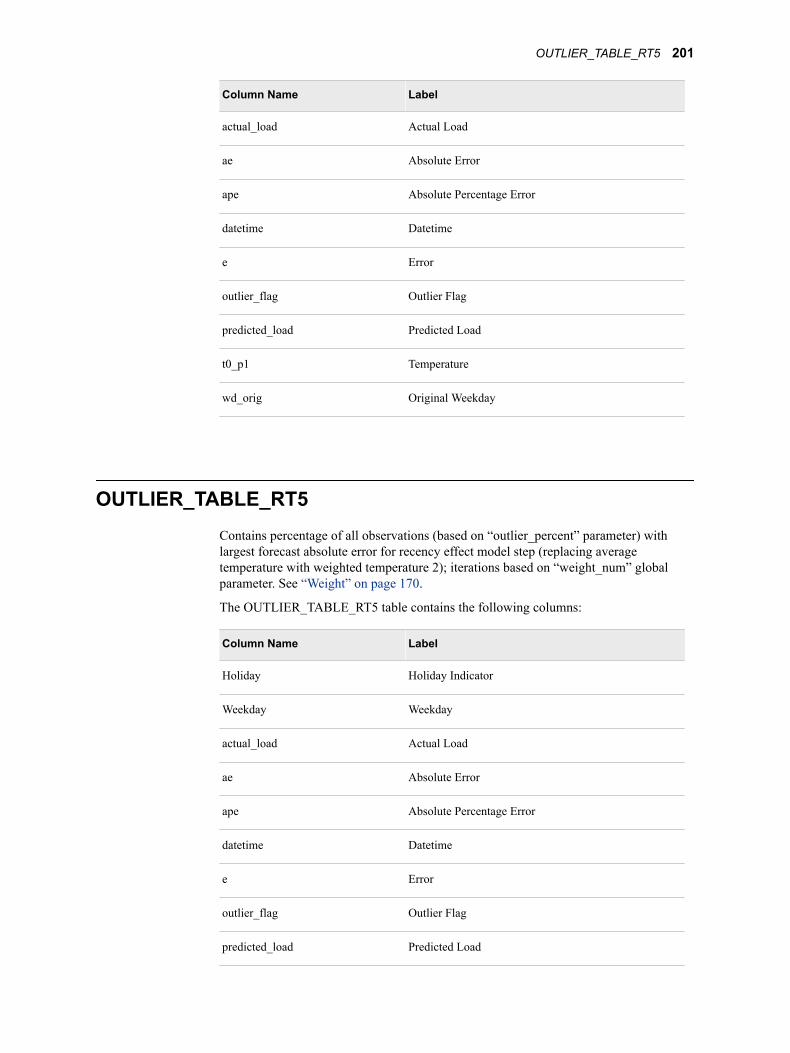
Column Name Label


ae Absolute Error


datetime Datetime

e Error



t0_p1 Temperature




Column Name Label


Weekday Weekday


ae Absolute Error


datetime Datetime

e Error




Column Name Label

t0_p1 Temperature




Column Name Label


Weekday Weekday


ae Absolute Error


datetime Datetime

e Error



t0_p1 Temperature





Column Name Label


Weekday Weekday


ae Absolute Error


datetime Datetime

e Error



t0_p1 Temperature


OUTLIER_TABLE_WEEKENDContains percentage of all observations (based on “outlier_percent” parameter) with largest forecast absolute error for weekend effect model

The OUTLIER_TABLE_WEEKEND table contains the following columns:

Column Name Label


Weekday Weekday


ae Absolute Error


datetime Datetime

e Error

OUTLIER_TABLE_WEEKEND 203

Column Name Label



t0_p1 Temperature


OUTLIER_TABLE_WLSContains percentage of all observations (based on “outlier_percent” parameter) with largest forecast absolute error for WLS model (weighted least squares)

The OUTLIER_TABLE_WLS table contains the following columns:

Column Name Label


Weekday Weekday


ae Absolute Error


datetime Datetime

e Error



t0_p1 Temperature


PARAMETER_CONTROL_CTStores some macro variables used by VSEL (value selection). These values will be passed to STLF, VSTLF, and MTLF/LTLF programs


The PARAMETER_CONTROL_CT table contains the following columns:

Column Name Label

Best_Model Best Model

FS Friday Saturday

MS Sunday Monday

MT Monday Tuesday

SS Saturday Sunday

TF Thursday Friday

TW Tuesday Wednesday

WT Wednesday Thursday

airport Airport

holiday_override Holiday Override

mape Mean Absolute Percentage Error

num_cpu Number of Parallel Processes to Run

rolling_end_date Rolling End Date

rolling_start_date Rolling Start Date

single_temp_code Single Temp Code

sub_date_offset Number of Days Between the Submission Date and the Forecast Date

sub_hour Hour Submission

train_start_date Start data of history

utility Utility

w_annual_mape Weighted Annual Mean Absolute Percentage Error

This is the weight assigned to annual energy MAPE in calculating weighted_mape.

w_annual_peak_mape Weighted Annual Peak Mean Absolute Percentage Error

This is the weight assigned to annual peak MAPE in calculating weighted_mape.

PARAMETER_CONTROL_CT 205

Column Name Label

w_daily_mape Weighted Daily Mean Absolute Percentage Error

This is the weight assigned to daily energy MAPE in calculating weighted_mape.

w_daily_peak_mape Weighted Daily Peak Mean Absolute Percentage Error

This is the weight assigned to daily peak MAPE in calculating weighted_mape.

w_hourly_mape Weighted Hourly Mean Absolute Percentage Error

This is the weight assigned to hourly MAPE in calculating weighted_mape.

w_monthly_mape Weighted Monthly Mean Absolute Percentage Error

This is the weight assigned to monthly energy MAPE in calculating weighted_mape.

w_monthly_peak_mape Weighted Monthly Peak Mean Absolute Percentage Error

This is the weight assigned to monthly peak MAPE in calculating weighted_mape.

weight_lower Lower Boundary of the Weight Used to Calculate the Exponentially Smoothed Temperature

weight_num The Number of Weights to Calculate Exponentially Smoothed Temperature

weight_upper Upper Boundary of the Weight Used to Calculate the Exponentially Smoothed Temperature

weighted_temp_code Weighted Temp Code

wls_weight Weight Least Square Model Weight


Part 5

Very Short Term Load Forecasting

Chapter 22Parameters for Very Short Term Load Forecasting . . . . . . . . . . . . . . . 209

Chapter 23The Very Short Term Forecasting Process . . . . . . . . . . . . . . . . . . . . . . . 215

Chapter 24Very Short Term Forecast Result Files . . . . . . . . . . . . . . . . . . . . . . . . . . 219

207

Chapter 22

Parameters for Very Short Term Load Forecasting

Main Parameters . . . . . . . . . . . . . . . . . . . . . . . . . . . . . . . . . . . . . . . . . . . . . . . . . . . . 209Historical Start Date . . . . . . . . . . . . . . . . . . . . . . . . . . . . . . . . . . . . . . . . . . . . . . . . 209Forecast Start Date . . . . . . . . . . . . . . . . . . . . . . . . . . . . . . . . . . . . . . . . . . . . . . . . . 210Forecast Start Hour . . . . . . . . . . . . . . . . . . . . . . . . . . . . . . . . . . . . . . . . . . . . . . . . . 210Forecast Length . . . . . . . . . . . . . . . . . . . . . . . . . . . . . . . . . . . . . . . . . . . . . . . . . . . 210

Report Data Parameters . . . . . . . . . . . . . . . . . . . . . . . . . . . . . . . . . . . . . . . . . . . . . . 210Reporting Mart . . . . . . . . . . . . . . . . . . . . . . . . . . . . . . . . . . . . . . . . . . . . . . . . . . . . 210Reporting SAS Data Model . . . . . . . . . . . . . . . . . . . . . . . . . . . . . . . . . . . . . . . . . . 211HANA Server . . . . . . . . . . . . . . . . . . . . . . . . . . . . . . . . . . . . . . . . . . . . . . . . . . . . . 211HANA Instance . . . . . . . . . . . . . . . . . . . . . . . . . . . . . . . . . . . . . . . . . . . . . . . . . . . . 211HANA Schema . . . . . . . . . . . . . . . . . . . . . . . . . . . . . . . . . . . . . . . . . . . . . . . . . . . . 211HANA Authentication Domain . . . . . . . . . . . . . . . . . . . . . . . . . . . . . . . . . . . . . . . 212

System Parameters . . . . . . . . . . . . . . . . . . . . . . . . . . . . . . . . . . . . . . . . . . . . . . . . . . . 212Forecast Initialization Exit . . . . . . . . . . . . . . . . . . . . . . . . . . . . . . . . . . . . . . . . . . . 212Reporting Exit . . . . . . . . . . . . . . . . . . . . . . . . . . . . . . . . . . . . . . . . . . . . . . . . . . . . . 212Forecast Completion Exit . . . . . . . . . . . . . . . . . . . . . . . . . . . . . . . . . . . . . . . . . . . . 212

Enable Event Listening to Run in Batch . . . . . . . . . . . . . . . . . . . . . . . . . . . . . . . . . 213

Main Parameters

Historical Start DateSelect the start date for historical date that is to be used for creating the forecast.

209

Note: The forecast start date should be at least 12 months later than the historical start date—a full year of history is required for making a forecast.

Column name in table: hist_start_date

Forecast Start DateSelect the start date for the forecast horizon.

Note: The forecast start date should be at least 12 months later than the historical start date—a full year of historical data is required for making a forecast.

Column name in table: fcst_start_date

Forecast Start HourSelect the start hour for the forecast horizon (between 1 and 24).

Column name in table: fcst_start_hour

Forecast LengthSelect the length for the forecast horizon, which is the number of hours to be forecasted (integer value).

Column name in table: fcst_length

Report Data Parameters

Reporting MartIn addition to the regular diagnose and forecast results, you can request data to be outputted in a form that is suitable for producing reports with SAS Visual Analytics, HANA, or another reporting tool. This report data is created by selecting fields from the individual diagnose and forecast result tables. You can request:

SASReport data outputted as SAS data sets

HANAReport data outputted as HANA tables

210 Chapter 22 • Parameters for Very Short Term Load Forecasting

NONENo report data is outputted. Only the regular diagnose and forecast results are outputted.

Column name in table: reporting_mart

Reporting SAS Data ModelIf, in the Reporting Mart field, you select report data to be outputted for either SAS or HANA, then select how the report data is outputted:

Normalizedto produce more tables but smaller ones which you must join for reporting purposes. If you select HANA for your report output, then the tables are automatically Normalized.

Denormalizedto produce fewer tables but larger ones. If you select SAS to output SAS data sets for use with SAS Visual Analytics, then you can select either Normalized or Denormalized.

Note: If you select Denormalized, then the amount of storage space required can grow very quickly. Make sure periodically to purge your files so as not to stress the system.

BothBoth normalized and denormalized files are outputted.

Note: This option applies only if you selected SAS in the Reporting Mart field. If you selected HANA, then the Normalized option is assumed.

For information, see Chapter 11, “Produce Reports,” on page 83.

Column name in table: reporting_sas_data_model


For information, see Chapter 13, “Work with SAP HANA,” on page 117.

Column name in table: hana_server.



Column name in table: hana_instance.


For information, see “Step 3. Create a SAP HANA Schema” on page 125.

Column name in table: hana_schema.

Report Data Parameters 211


For general information, see Chapter 13, “Work with SAP HANA,” on page 117.

More specifically, see Step 6b on page 122.

Column name in table: hana_authentication.

System Parameters

Forecast Initialization ExitThis parameter is reserved for internal SAS use only.

Specify the path and file name of a SAS program or macro that SAS Energy Forecasting will invoke before the forecast is run. For example: C:\hana\init.sas.

Typically, you can use such a program to allocate resources and connections that you need to run the forecast.

Note: If you specify such a program, then you probably want also to specify a program with Forecast Completion Exit to free the resources and connections made during initialization.

Column name in table: sefvs_init_exit.xml

Reporting ExitThis parameter is reserved for internal SAS use only.

Specify the path and file name of a SAS program or macro that SAS Energy Forecasting will invoke after the forecast is run but before data is written out either to SAS data sets or to a SAP HANA for reporting. For example: C:\hana\report.sas.

Column name in table: sefvs_rpt_exit.xml

Forecast Completion ExitThis parameter is reserved for internal SAS use only.

Specify the path and file name of a SAS program or macro that SAS Energy Forecasting will invoke after the forecast is finished. For example: C:\hana\terminate.sas.


Typically, you can use such a program to free resources and connections that you made with your program specified in Forecast Initialization Exit.

Column name in table: sefvs_term_exit.xml

Enable Event Listening to Run in BatchIf you select Enable Event Listening for a forecast, then you can run it from the data tier by using the macro %sefdatae without having to open to the SAS Energy Forecasting client. The macro includes information as to which forecasts are to be run of those for which Enable Event Listening is selected

Typically, you might run the macro after updating input data for a forecast. You can select Enable Event Listening for any forecast.

See AlsoChapter 10, “Run in Batch,” on page 79

Enable Event Listening to Run in Batch 213

Chapter 23

The Very Short Term Forecasting Process

One-Stage Model . . . . . . . . . . . . . . . . . . . . . . . . . . . . . . . . . . . . . . . . . . . . . . . . . . . . . 215

Two-Stage Model . . . . . . . . . . . . . . . . . . . . . . . . . . . . . . . . . . . . . . . . . . . . . . . . . . . . 217

One-Stage ModelThe modeling methodology for VSTLF (very short term load forecasting) is as follows:

Data pre-processingThe “parameter_control” table (“PARAMETER_CONTROL_CT” on page 204) and the holiday look-up table (“HOLIDAY_LKP_CT” on page 194) are generated from the diagnose process. (See Chapter 20, “The Diagnose Process,” on page 185.) The VSTLF code uses the parameters read from the “parameter_control” table to set the recency and weekend effects.

ForecastingIf the selected best model from the diagnose process is not the WLS holiday model, VSTLF uses the selected best model as the base model and the lag load of the previous hour is added to it. Otherwise, VSTLF uses the second-best model as the base model and the lag load of the previous hour is added to it. For example, if the selected best model for STLF is the naïve model, the model for VSTLF would be as follows (Equation VSTN1):

If the forecasting horizon is more than one hour, the forecasted load is used to forecast the next hour’s load, instead of the actual load. However, the forecasted load becomes more and more inaccurate as the forecasting horizon gets longer. If the lag load is included, it should be available when doing forecasting.

The following table summarizes the very short term modeling methodology.

Temperature Updating cycle Horizon

Required <= 1 hour Within 1 day

215

Example 1: One-Hour-Ahead ForecastingThe following example explains why the lag load is required. If it is some point between 7:00 a.m. and 8:00 a.m. and a forecast for 9:00 a.m. for that particular day using the “VSTN1” model is desired, all time points prior to and at 7:00 a.m. of Day 1 have historical load data but all time points after 7:00 a.m. of Day 1have no historical load data. The “VSTN1” model includes the load for the previous hour, so the load for 8:00 a.m. should be available if the load for 9:00 a.m. is being forecasted. The actual load for 8:00 a.m. is of course not available for a 9:00 a.m. forecast, so the following procedure should be followed:

1. Forecast the load at 8:00 a.m. using historical load data.

2. Use the forecast load for 8:00 a.m. as load(t-1) in the “VSTN1” model along with the historical load to forecast the load for 9:00 a.m.

... Day 1, 7:00 a.m. Day 1, 8:00 a.m. Day 1, 9:00 a.m. Day 1, 10:00 a.m. Day 1, 11:00 a.m.

Historical data is available

Current time point Future time point Future time point Future time point Future time point

Example 2: One-Day-Ahead ForecastingIf it is some point between 7:00 a.m. and 8:00 a.m. of Day 1 and forecasts for every hour of Day 2 using the “VSTN1” model are desired, the following procedure should be followed:

1. Forecast the load at 8:00 a.m. of Day 1 using historical load data.

2. Use the forecast load for 8:00 a.m. of Day 1 as load(t-1) in the “VSTN1” model along with the historical load to forecast the load for 9:00 a.m. of Day 1.


4. Use the forecast load for 11:00 p.m. of Day 1 as load(t-1) in the “VSTN1” model along with the historical load to forecast the load for midnight of Day 2.

5. Use the forecast load for midnight of Day 2 as load(t-1) in the “VSTN1” model along with the historical load to forecast the load for 1:00 a.m. of Day 2.


7. Use the forecast load for 11:00 p.m. of Day 2 as load(t-1) in the “VSTN1” model along with the historical load to forecast the load for midnight of Day 3.

This procedure does one hour ahead for each hour of Day 2, a total of 24 calculations. At the end of it, the forecast load for every hour of Day 2 (a complete “day”) has been obtained.

216 Chapter 23 • The Very Short Term Forecasting Process

...Day 1, 7:00 a.m.

Day 1, 8:00 a.m.

Day 1, 9:00 a.m. Day 1, ...

Day 2, 1:00 a.m.

Day 2, 2:00 a.m. Day 2, ...

Day 3, midnight

Historical data is available

Current time point

Future time point

Future time point

Future time point

Future time point

Future time point

Future time point

Future time point

Two-Stage ModelIf the best model from the two-stage diagnose process is one of the two-stage models (GLM_UCM, GLM_NN, GLM_ESM, or GLM_ARIMAX), the load (GLM) and the residual (UCM, neural network, ESM, or ARIMAX model) are forecasted and then added together to generate the final predicted load. Otherwise, the onestage model method is utilized to forecast the load (“One-Stage Model” on page 215).

Two-Stage Model 217

218 Chapter 23 • The Very Short Term Forecasting Process

Chapter 24

Very Short Term Forecast Result Files

FCST_RESULTS . . . . . . . . . . . . . . . . . . . . . . . . . . . . . . . . . . . . . . . . . . . . . . . . . . . . 219

FCST_RESULTS_ALL . . . . . . . . . . . . . . . . . . . . . . . . . . . . . . . . . . . . . . . . . . . . . . . 219

FCST_STAT . . . . . . . . . . . . . . . . . . . . . . . . . . . . . . . . . . . . . . . . . . . . . . . . . . . . . . . . 220

GLM_PARAMS . . . . . . . . . . . . . . . . . . . . . . . . . . . . . . . . . . . . . . . . . . . . . . . . . . . . . 221

OUTLIER_GLM . . . . . . . . . . . . . . . . . . . . . . . . . . . . . . . . . . . . . . . . . . . . . . . . . . . . 222

OUTLIER_GLM_W1 . . . . . . . . . . . . . . . . . . . . . . . . . . . . . . . . . . . . . . . . . . . . . . . . 222

OUTLIER_GLM_W2 . . . . . . . . . . . . . . . . . . . . . . . . . . . . . . . . . . . . . . . . . . . . . . . . 223

OUTLIER_GLM_W3 . . . . . . . . . . . . . . . . . . . . . . . . . . . . . . . . . . . . . . . . . . . . . . . . 224

OUTLIER_GLM_W4 . . . . . . . . . . . . . . . . . . . . . . . . . . . . . . . . . . . . . . . . . . . . . . . . 224

OUTLIER_GLM_WLS . . . . . . . . . . . . . . . . . . . . . . . . . . . . . . . . . . . . . . . . . . . . . . . 225

FCST_RESULTSContains forecast results for best chosen model


Column Name Label

Datetime Datetime

He Hour


FCST_RESULTS_ALLContains forecast results for:

• GLM

219

• GLM two-stage (depends on if two-stage models are enabled and the best model from diagnose process )

• COMBINE model (depends on if two-stage models are enabled and the best model from diagnose process)

• WLS (weighted least squares) model(only if “wls” parameter =yes)

Column Name Label

date Date

datetime Datetime

he Hour

predicted_load_2stage Predicted Load Two Stage

predicted_load_GLM Predicted Load GLM

predicted_load_GLM_WLS Predicted Load GLMWLS

FCST_STATContains forecast statistics for:

• GLM

• GLM two-stage models (depends on if two-stage models are enabled and the best model from diagnose process)


• WLS (weighted least squares) model (only if “wls” parameter =yes)

Statistics include MAE, MAPE, and ME for annual energy, annual peak load, daily energy, daily peak load, monthly energy, monthly peak load, and hourly load


Column Name Label






220 Chapter 24 • Very Short Term Forecast Result Files

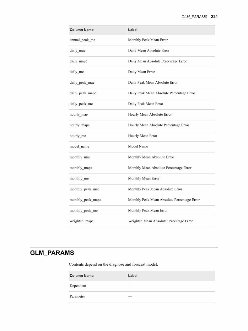
Column Name Label



















GLM_PARAMSContents depend on the diagnose and forecast model.

Column Name Label

Dependent —

Parameter —

GLM_PARAMS 221

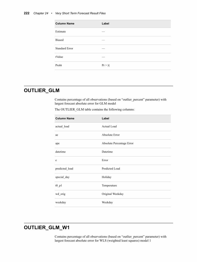
Column Name Label

Estimate —

Biased —

Standard Error —

tValue —

Probt Pr > |t|

OUTLIER_GLMContains percentage of all observations (based on “outlier_percent” parameter) with largest forecast absolute error for GLM model

The OUTLIER_GLM table contains the following columns:

Column Name Label


ae Absolute Error


datetime Datetime

e Error


special_day Holiday

t0_p1 Temperature


weekday Weekday

OUTLIER_GLM_W1Contains percentage of all observations (based on “outlier_percent” parameter) with largest forecast absolute error for WLS (weighted least squares) model 1


The OUTLIER_GLM_W1 table contains the following columns:

Column Name Label


ae Absolute Error


datetime Datetime

e Error


special_day Holiday

t0_p1 Temperature


weekday Weekday



Column Name Label


ae Absolute Error


datetime Datetime

e Error


special_day Holiday

t0_p1 Temperature

OUTLIER_GLM_W2 223

Column Name Label


weekday Weekday



Column Name Label


ae Absolute Error


datetime Datetime

e Error


special_day Holiday

t0_p1 Temperature


weekday Weekday

OUTLIER_GLM_W4Contains percentage of all observations (based on “outlier_percent” parameter) with largest forecast absolute error for WLS (weighted least squares)model 4


Column Name Label



Column Name Label

ae Absolute Error


datetime Datetime

e Error


special_day Holiday

t0_p1 Temperature


weekday Weekday

OUTLIER_GLM_WLSContains percentage of all observations (based on “outlier_percent” parameter) with largest forecast absolute error for WLS (weighted least squares) model

The OUTLIER_GLM_WLS table contains the following columns:

Column Name Label


ae Absolute Error


datetime Datetime

e Error


special_day Holiday

t0_p1 Temperature


weekday Weekday

OUTLIER_GLM_WLS 225

Part 6

Short Term Load Forecasting

Chapter 25Parameters for Short Term Load Forecasting . . . . . . . . . . . . . . . . . . . . 229

Chapter 26The Short Term Forecasting Process . . . . . . . . . . . . . . . . . . . . . . . . . . . . 235

Chapter 27Short Term Forecast Result Files . . . . . . . . . . . . . . . . . . . . . . . . . . . . . . . 237

227

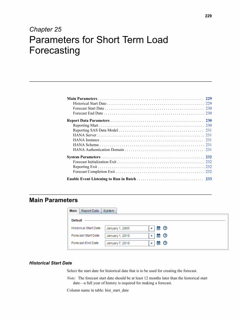
Chapter 25

Parameters for Short Term Load Forecasting

Main Parameters . . . . . . . . . . . . . . . . . . . . . . . . . . . . . . . . . . . . . . . . . . . . . . . . . . . . 229Historical Start Date . . . . . . . . . . . . . . . . . . . . . . . . . . . . . . . . . . . . . . . . . . . . . . . . 229Forecast Start Date . . . . . . . . . . . . . . . . . . . . . . . . . . . . . . . . . . . . . . . . . . . . . . . . . 230Forecast End Date . . . . . . . . . . . . . . . . . . . . . . . . . . . . . . . . . . . . . . . . . . . . . . . . . . 230

Report Data Parameters . . . . . . . . . . . . . . . . . . . . . . . . . . . . . . . . . . . . . . . . . . . . . . 230Reporting Mart . . . . . . . . . . . . . . . . . . . . . . . . . . . . . . . . . . . . . . . . . . . . . . . . . . . . 230Reporting SAS Data Model . . . . . . . . . . . . . . . . . . . . . . . . . . . . . . . . . . . . . . . . . . 231HANA Server . . . . . . . . . . . . . . . . . . . . . . . . . . . . . . . . . . . . . . . . . . . . . . . . . . . . . 231HANA Instance . . . . . . . . . . . . . . . . . . . . . . . . . . . . . . . . . . . . . . . . . . . . . . . . . . . 231HANA Schema . . . . . . . . . . . . . . . . . . . . . . . . . . . . . . . . . . . . . . . . . . . . . . . . . . . . 231HANA Authentication Domain . . . . . . . . . . . . . . . . . . . . . . . . . . . . . . . . . . . . . . . 231



Main Parameters

Historical Start DateSelect the start date for historical date that is to be used for creating the forecast.

Note: The forecast start date should be at least 12 months later than the historical start date—a full year of history is required for making a forecast.

Column name in table: hist_start_date

229

Forecast Start DateSelect the start date for the forecast horizon.

Note: The forecast start date should be at least 12 months later than the historical start date—a full year of historical data is required for making a forecast.

Column name in table: fcst_start_date

Forecast End DateSelect the end date for the forecast horizon, which should be:

• the same as or later than the start date for the forecast horizon

• and less than or equal to the end date of the temperature data.

The load to the last hour of this day is forecasted.

Column name in table: fcst_end_date







230 Chapter 25 • Parameters for Short Term Load Forecasting




















Report Data Parameters 231



System Parameters





Column name in table: sefsh_init_exit.xml



Column name in table: sefsh_rpt_exit.xml




Column name in table: sefsh_term_exit.xml





Enable Event Listening to Run in Batch 233

Chapter 26

The Short Term Forecasting Process

One-Stage Model . . . . . . . . . . . . . . . . . . . . . . . . . . . . . . . . . . . . . . . . . . . . . . . . . . . . . 235

Two-Stage Model . . . . . . . . . . . . . . . . . . . . . . . . . . . . . . . . . . . . . . . . . . . . . . . . . . . . 235

One-Stage ModelThe modeling methodology for short term load forecasting is as follows:

Data pre-processingThe “parameter_control” table (“PARAMETER_CONTROL_CT” on page 204) and the holiday look-up table (“HOLIDAY_LKP_CT” on page 194) are generated from the diagnose process. (See Chapter 20, “The Diagnose Process,” on page 185.) The short term load forecasting code uses the parameters read from the “parameter_control” table to set the recency and weekend effects.

ForecastingThe short term load forecasting code (ulf_stlf.sas) runs a generalized linear model (GLM) with the pre-processed data in order to forecast the specified short term load forecasting.

The following table summarizes the short term modeling methodology.

Temperature Updating cycle Horizon

Required 1 day 1 day to 2 weeks

Two-Stage ModelIf the best model from the two-stage diagnose process is one of the two-stage models (GLM_UCM, GLM_NN, GLM_ESM, or GLM_ARIMAX), the load (GLM) and the residual (UCM, neural network, ESM, or ARIMAX model) are forecasted and then added together to generate the final predicted load. Otherwise, the one-stage model method is utilized to forecast the load (“One-Stage Model” on page 235).

235

236 Chapter 26 • The Short Term Forecasting Process

Chapter 27

Short Term Forecast Result Files

FCST_RESULTS . . . . . . . . . . . . . . . . . . . . . . . . . . . . . . . . . . . . . . . . . . . . . . . . . . . . 237

FCST_RESULTS_ALL . . . . . . . . . . . . . . . . . . . . . . . . . . . . . . . . . . . . . . . . . . . . . . . 237

FCST_STAT . . . . . . . . . . . . . . . . . . . . . . . . . . . . . . . . . . . . . . . . . . . . . . . . . . . . . . . . 238

GLM_PARAMS . . . . . . . . . . . . . . . . . . . . . . . . . . . . . . . . . . . . . . . . . . . . . . . . . . . . . 239

FCST_RESULTSContains forecast results for best chosen model


Column Name Label

date Date

datetime Datetime

he Hour


FCST_RESULTS_ALLContains forecast results for:

• GLM model

• GLM two-stage model (depends on if two-stage models are enabled and the best model from diagnose process) and/or:


237

Column Name Label

date Date

datetime Datetime

he Hour

predicted_load Predicted Load GLM

predicted_load_2stage Predicted Load Two Stage

FCST_STATContains forecast statistics for:

• GLM

• GLM two-stage models (depends on if two-stage models are enabled and the best model from diagnose process) and/or:


Statistics include MAE, MAPE, and ME for annual energy, annual peak load, daily energy, daily peak load, monthly energy, monthly peak load, and hourly load


Column Name Label











238 Chapter 27 • Short Term Forecast Result Files

Column Name Label















Column Name Label

Dependent —

Parameter —

Estimate —

Biased —

Standard Error —

tValue —

Probt Pr > |t|

GLM_PARAMS 239

240 Chapter 27 • Short Term Forecast Result Files

Part 7

Medium Term and Long Term Load Forecasting

Chapter 28Parameters for Medium Term and Long Term Load Forecasting . . 243

Chapter 29The Medium Term/Long Term Forecasting Process . . . . . . . . . . . . . . 249

Chapter 30Medium Term/Long Term Forecast Result Files . . . . . . . . . . . . . . . . . . 251

241

Chapter 28

Parameters for Medium Term and Long Term Load Forecasting

Main Parameters . . . . . . . . . . . . . . . . . . . . . . . . . . . . . . . . . . . . . . . . . . . . . . . . . . . . 244Historical T Start . . . . . . . . . . . . . . . . . . . . . . . . . . . . . . . . . . . . . . . . . . . . . . . . . . . 244Historical T End . . . . . . . . . . . . . . . . . . . . . . . . . . . . . . . . . . . . . . . . . . . . . . . . . . . 244Historical Load Start Date . . . . . . . . . . . . . . . . . . . . . . . . . . . . . . . . . . . . . . . . . . . 244Historical Load End Date . . . . . . . . . . . . . . . . . . . . . . . . . . . . . . . . . . . . . . . . . . . . 245Forecast End Date . . . . . . . . . . . . . . . . . . . . . . . . . . . . . . . . . . . . . . . . . . . . . . . . . . 245Number of Scenarios . . . . . . . . . . . . . . . . . . . . . . . . . . . . . . . . . . . . . . . . . . . . . . . 245MLT Assumption . . . . . . . . . . . . . . . . . . . . . . . . . . . . . . . . . . . . . . . . . . . . . . . . . . 245

Report Data Parameters . . . . . . . . . . . . . . . . . . . . . . . . . . . . . . . . . . . . . . . . . . . . . . 246Reporting Mart . . . . . . . . . . . . . . . . . . . . . . . . . . . . . . . . . . . . . . . . . . . . . . . . . . . . 246Reporting SAS Data Model . . . . . . . . . . . . . . . . . . . . . . . . . . . . . . . . . . . . . . . . . . 246HANA Server . . . . . . . . . . . . . . . . . . . . . . . . . . . . . . . . . . . . . . . . . . . . . . . . . . . . . 247HANA Instance . . . . . . . . . . . . . . . . . . . . . . . . . . . . . . . . . . . . . . . . . . . . . . . . . . . 247HANA Schema . . . . . . . . . . . . . . . . . . . . . . . . . . . . . . . . . . . . . . . . . . . . . . . . . . . . 247HANA Authentication Domain . . . . . . . . . . . . . . . . . . . . . . . . . . . . . . . . . . . . . . . 247



243

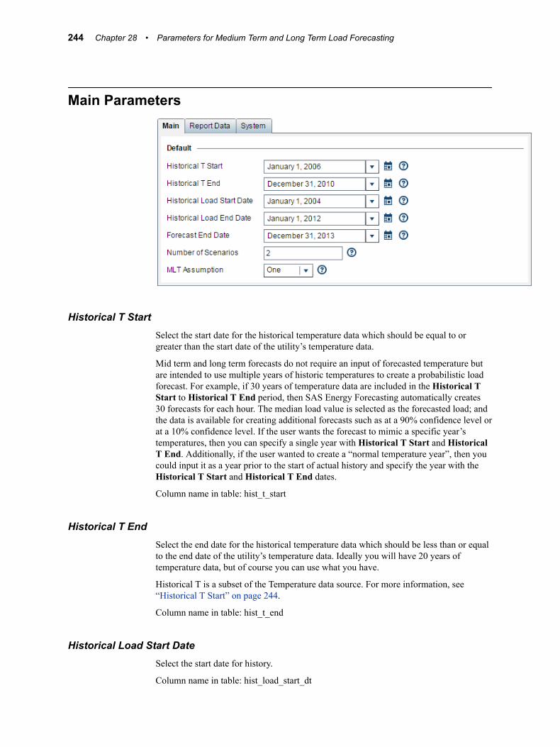
Main Parameters

Historical T StartSelect the start date for the historical temperature data which should be equal to or greater than the start date of the utility’s temperature data.

Mid term and long term forecasts do not require an input of forecasted temperature but are intended to use multiple years of historic temperatures to create a probabilistic load forecast. For example, if 30 years of temperature data are included in the Historical T Start to Historical T End period, then SAS Energy Forecasting automatically creates 30 forecasts for each hour. The median load value is selected as the forecasted load; and the data is available for creating additional forecasts such as at a 90% confidence level or at a 10% confidence level. If the user wants the forecast to mimic a specific year’s temperatures, then you can specify a single year with Historical T Start and Historical T End. Additionally, if the user wanted to create a “normal temperature year”, then you could input it as a year prior to the start of actual history and specify the year with the Historical T Start and Historical T End dates.

Column name in table: hist_t_start

Historical T EndSelect the end date for the historical temperature data which should be less than or equal to the end date of the utility’s temperature data. Ideally you will have 20 years of temperature data, but of course you can use what you have.

Historical T is a subset of the Temperature data source. For more information, see “Historical T Start” on page 244.

Column name in table: hist_t_end

Historical Load Start DateSelect the start date for history.

Column name in table: hist_load_start_dt

244 Chapter 28 • Parameters for Medium Term and Long Term Load Forecasting

Historical Load End DateSelect the end date for history. Set the end date to be at least 12 months after the start date—one year of historical data is required.

Column name in table: hist_load_end_dt

Forecast End DateSelect the end date for the forecast horizon, which should be:

• the same as or later than the start date for the forecast horizon

• and less than or equal to the end date of the economic data.

The load to the last hour of this day is forecasted.

Column name in table: fcst_end_date

Number of ScenariosEnter the number of economy scenarios to be used (an integer between 1 and 7, with a default of 7). Specifying 1 means to use the first scenario. Specifying 2 means to use the first two.

Column name in table: num_scenarios

MLT AssumptionThis parameter is used to set how GXP (gross x product) will be included in the forecast model. The values can be 1, 2 or 3 which represent one of the following:

• 1=Include GXP as Trend

• 2=Include GXP as Trend and Interact GXP with other factors

• 3=Divide Load by GXP

Column name in table: mtlt_assumption

See “Medium Term / Long Term Forecasting” on page 249.

Main Parameters 245


















System Parameters

System Parameters 247





Column name in table: sefml_init_exit.xml



Column name in table: sefml_rpt_exit.xml




Column name in table: sefml_term_exit.xml





Chapter 29

The Medium Term/Long Term Forecasting Process

Medium Term / Long Term Forecasting . . . . . . . . . . . . . . . . . . . . . . . . . . . . . . . . . . 249

Medium Term / Long Term ForecastingThe diagnose process parameter setup and processing for MTLF is the same as that for STLF except that MTLF diagnose does not need to process two-stage and WLS models.

The MTLF process selects the best model information from the diagnose process and generates a forecast for middle-term.

The modeling methodology for MTLF/LTLF is as follows:

1. Run the diagnose process (see Chapter 20, “The Diagnose Process,” on page 185) and assume that the best model is as follows (Base equation):

2. Replace the trend with gross x product (GxP) and interact GxP with all variables. This yields the “ML1” model.

Assuming that 10 years of historical hourly temperature, load, and economic data is available, it can be used to estimate the “ML1” model. In general, there is annual, quarterly, or monthly economic data, which means that the same economic data is used for every hour, as follows (Equation ML1):

Other aspects of the MTLF/LTLF methodology are as follows:

• For a national utility, GxP can be gross domestic product

• For a cross-state utility or state power system, GxP can be gross state product

• For a utility with service territory covering a metropolitan area, GxP can be gross metropolitan product.

249

Historical weather scenarios and economic forecasts are used to simulate normal loads, as follows:

• Assuming that there are 50 years of historical hourly weather data (1960 – 2010), the “ML1” model can be used to do forecasting under 50 scenarios; at the very least, 30 years of historical weather data should be available

• In general, economic forecasts provide several different scenarios (e.g., base, strong rebound, slower recovery, and double-dip recession); forecasts are run under each economy scenario.

For example, 50 forecasts can be generated under the base economy scenario, as shown in a table such as the one below. For each economy scenario, forecasts are simulated using each year of weather data for 50 years (1960 – 2010) as the weather for 2012 – 2041 (30 years of forecasts using 50 years of weather data). The median of these 50 forecasts is the normal load under the base economy scenario, which is known as weather normalization. Users of SAS Energy Forecasting should be able to choose how many years of historical weather data they would like to use, but at least 30 years of historical weather data should be used.

gxp_base *temp_1960 gxp_base *temp_1961 … gxp_base *temp_2010

01Jan201 1 01 — — — —

01Jan201 1 02 — — — —

01Jan201 1 03 — — — —

01Jan201 1 04 — — — —

... — — — —

The following table summarizes the long term and medium term modeling methodology.

Temperature Economics Updating cycle Horizon

Medium Term LF Simulated Required 1 month 1 – 3 years

Long Term LF Simulated Required 1 year 30 years or up

250 Chapter 29 • The Medium Term/Long Term Forecasting Process

Chapter 30

Medium Term/Long Term Forecast Result Files

ANNUAL_PEAK_STAT_NAIVE_0 . . . . . . . . . . . . . . . . . . . . . . . . . . . . . . . . . . . . . 252







FCST_RESULTS_ML_HOLIDAY_0 . . . . . . . . . . . . . . . . . . . . . . . . . . . . . . . . . . . . 256

FCST_RESULTS_ML_NAIVE_0 . . . . . . . . . . . . . . . . . . . . . . . . . . . . . . . . . . . . . . . 256

FCST_RESULTS_ML_RECENCY_0 . . . . . . . . . . . . . . . . . . . . . . . . . . . . . . . . . . . 257

FCST_RESULTS_ML_WEEKEND_0 . . . . . . . . . . . . . . . . . . . . . . . . . . . . . . . . . . . 258

GLM_PARAMS . . . . . . . . . . . . . . . . . . . . . . . . . . . . . . . . . . . . . . . . . . . . . . . . . . . . . 258

GLM_PARAMS_ML_HOLIDAY_0 . . . . . . . . . . . . . . . . . . . . . . . . . . . . . . . . . . . . . 259

GLM_PARAMS_ML_HOLIDAY_1 . . . . . . . . . . . . . . . . . . . . . . . . . . . . . . . . . . . . . 259

GLM_PARAMS_ML_NAIVE_0 . . . . . . . . . . . . . . . . . . . . . . . . . . . . . . . . . . . . . . . . 260

GLM_PARAMS_ML_NAIVE_1 . . . . . . . . . . . . . . . . . . . . . . . . . . . . . . . . . . . . . . . . 260

GLM_PARAMS_ML_RECENCY_0 . . . . . . . . . . . . . . . . . . . . . . . . . . . . . . . . . . . . 261

GLM_PARAMS_ML_RECENCY_1 . . . . . . . . . . . . . . . . . . . . . . . . . . . . . . . . . . . . 261

GLM_PARAMS_ML_WEEKEND_0 . . . . . . . . . . . . . . . . . . . . . . . . . . . . . . . . . . . . 262

GLM_PARAMS_ML_WEEKEND_1 . . . . . . . . . . . . . . . . . . . . . . . . . . . . . . . . . . . . 262

HIST_FCST_RESULTS_ML_NAIVE_0 . . . . . . . . . . . . . . . . . . . . . . . . . . . . . . . . . 262

HIST_FCST_RESULTS_ML_RECENCY_0 . . . . . . . . . . . . . . . . . . . . . . . . . . . . . 263

HIST_FCST_RESULTS_ML_WEEKEND_0 . . . . . . . . . . . . . . . . . . . . . . . . . . . . . 264

HIST_FCST_RESULTS_ML_HOLIDAY_0 . . . . . . . . . . . . . . . . . . . . . . . . . . . . . . 264

251

ANNUAL_PEAK_STAT_NAIVE_0Contains annual peak load statistics for naïve model for economic scenario 0; statistics are summarized based on temperature scenarios taken from specified historical range

The ANNUAL_PEAK_STAT_NAIVE_0 table contains the following columns:

Column Name Label

MAX The Maximum Value

Mean The Arithmetic Mean

Median The Median Value

Min The Minimum Value

Num Number of Simulated Values

P10 The 10th Percentile


Year Year

actual_peak Actual Peak



Column Name Label






252 Chapter 30 • Medium Term/Long Term Forecast Result Files

Column Name Label



Year Year




Column Name Label








Year Year




ANNUAL_PEAK_STAT_NAIVE_3 253

Column Name Label








Year Year




Column Name Label








Year Year





Column Name Label








Year Year




Column Name Label






ANNUAL_PEAK_STAT_NAIVE_6 255

Column Name Label



Year Year


FCST_RESULTS_ML_HOLIDAY_0Contains the predicted load generated with various weather scenarios for holiday model for economic scenario 0

The FCST_RESULTS_ML_HOLIDAY_0 table contains the following columns:

Column Name Label

Datetime Datetime

Date Date

Hour Hour

Actual_load Actual Load

Year_orig Original Year

Year Year

Predicted_load Predicted load

Lower95 Lower 95 Confidence Interval

Upper95 Upper 95 Confidence Interv

FCST_RESULTS_ML_NAIVE_0Contains the predicted load generated with various weather scenarios for naïve model for economic scenario 0

The FCST_RESULTS_ML_NAIVE_0 table contains the following columns:


Column Name Label

Datetime Datetime

Date Date

Hour Hour



Year Year




FCST_RESULTS_ML_RECENCY_0Contains the predicted load generated with various weather scenarios for recency model for economic scenario 0

The FCST_RESULTS_ML_RECENCY_0 table contains the following columns:

Column Name Label

Datetime Datetime

Date Date

Hour Hour



Year Year




FCST_RESULTS_ML_RECENCY_0 257

FCST_RESULTS_ML_WEEKEND_0Contains the predicted load generated with various weather scenarios for weekend model for economic scenario 0

The FCST_RESULTS_ML_WEEKEND_0 table contains the following columns:

Column Name Label

Datetime Datetime

Date Date

Hour Hour



Year Year





Column Name Label

Dependent —

Parameter —

Estimate —

Biased —

Standard Error —

tValue —


Column Name Label

Probt Pr > |t|

GLM_PARAMS_ML_HOLIDAY_0

Column Name Label

Dependent —

Parameter —

Estimate —

Biased —

Standard Error —

tValue —

Probt Pr > |t|

GLM_PARAMS_ML_HOLIDAY_1

Column Name Label

Dependent —

Parameter —

Estimate —

Biased —

Standard Error —

tValue —

Probt Pr > |t|

GLM_PARAMS_ML_HOLIDAY_1 259

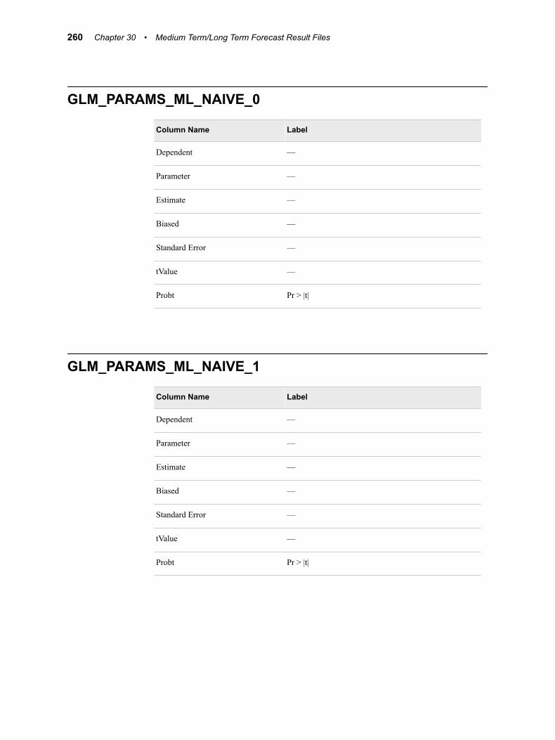
GLM_PARAMS_ML_NAIVE_0

Column Name Label

Dependent —

Parameter —

Estimate —

Biased —

Standard Error —

tValue —

Probt Pr > |t|

GLM_PARAMS_ML_NAIVE_1

Column Name Label

Dependent —

Parameter —

Estimate —

Biased —

Standard Error —

tValue —

Probt Pr > |t|


GLM_PARAMS_ML_RECENCY_0

Column Name Label

Dependent —

Parameter —

Estimate —

Biased —

Standard Error —

tValue —

Probt Pr > |t|

GLM_PARAMS_ML_RECENCY_1

Column Name Label

Dependent —

Parameter —

Estimate —

Biased —

Standard Error —

tValue —

Probt Pr > |t|

GLM_PARAMS_ML_RECENCY_1 261

GLM_PARAMS_ML_WEEKEND_0

Column Name Label

Dependent —

Parameter —

Estimate —

Biased —

Standard Error —

tValue —

Probt Pr > |t|

GLM_PARAMS_ML_WEEKEND_1

Column Name Label

Dependent —

Parameter —

Estimate —

Biased —

Standard Error —

tValue —

Probt Pr > |t|

HIST_FCST_RESULTS_ML_NAIVE_0Contains the predicted load generated with the actual weather scenario for naïve model for economic scenario 0


The HIST_FCST_RESULTS_ML_NAIVE_0 table contains the following columns:

Column Name Label

Datetime Datetime

Date Date

Hour Hour



Year Year




HIST_FCST_RESULTS_ML_RECENCY_0Contains the predicted load generated with the actual weather scenario for recency model for economic scenario 0

The HIST_FCST_RESULTS_ML_RECENCY_0 table contains the following columns:

Column Name Label

Datetime Datetime

Date Date

Hour Hour



Year Year




HIST_FCST_RESULTS_ML_RECENCY_0 263

HIST_FCST_RESULTS_ML_WEEKEND_0Contains the predicted load generated with the actual weather scenario for weekend model for economic scenario 0

The HIST_FCST_RESULTS_ML_WEEKEND_0 table contains the following columns:

Column Name Label

Datetime Datetime

Date Date

Hour Hour



Year Year




HIST_FCST_RESULTS_ML_HOLIDAY_0Contains the predicted load generated with the actual weather scenario for holiday model for economic scenario 0

The HIST_FCST_RESULTS_ML_HOLIDAY_0 table contains the following columns:

Column Name Label

Datetime Datetime

Date Date

Hour Hour




Column Name Label

Year Year




HIST_FCST_RESULTS_ML_HOLIDAY_0 265

sas energy forecasting 3.1: user's guide · 2016-12-20 · forecasting needs of the entire...

Documents