Chapter 3

Sampling and Sampled-Data

Systems

3.1 Introduction

Today, virtually all control systems are implemented digitally, on platformsthat range from large computer systems (e.g. the mainframe of an industrialSCADA1 system) to small embedded processors. Since computers work withdigital signals and the systems they control often live in the analog world, partof the engineered system must be responsible for converting the signals fromone domain to another. In particular, the control engineer should understandthe principles of sampling and quantization, and the basics of Analog to Digitaland Digital to Analog Converters (ADC and DAC).

Control systems that combine an analog part with some digital componentsare traditionally referred to as sampled-data systems. Alternative names suchas hybrid systems or cyber-physical systems (CPS) have also been used morerecently. In this case, the implied convention seems to be that the digitalpart of the system is more complex than in traditional sampled-data systems,involving in particular logic statements so that the system can switch betweendifferent behaviors. Another important concern for the development of CPSis system integration, since we must often assemble complex systems fromheterogeneous components that might be designed independently using perhapsdifferent modeling abstractions. In this chapter however we are concerned withthe classical theory of sampled-data system, and with digital systems that areassumed to be essentially dedicated to the control task, and as powerful forthis purpose as needed. Even in this case, interesting questions are raised bythe capabilities of modern digital systems, such as the possibility of very highsampling rates. Moreover, we can build on this theory to relax its unrealisticassumptions for modern embedded implementation platforms and to considermore complex hybrid system and CPS issues, as discussed in later chapters.

1SCADA = Supervisory Control and Data Acquisition

25

PhysicalContinuous-TimeSystem (Plant)

AAF QHS

disturbancesmeasurement

noise

digitalsignal

digitalsignal

ADC

Figure 3.1: Sampled-data model. H = hold, S = sampler, Q = quantizer (+decoder), AAF = anti-aliasing (low-pass) filter. Continuous-time signals arerepresented with full lines, discrete-time signals with dashed lines.

Organization of Sampled-Data Systems

The input signals of a digital controller consist of discrete sequences of finiteprecision numbers. We call such a sequence a digital signal. Often we ignorequantization (i.e., finite precision) issues and still call the discrete sequence adigital signal. In sampled-data systems, the plant to be controlled is an ana-log system (continuous-time, and usually continuous-state), and measurementsabout the state of this plant that are initially in the analog domain need tobe converted to digital signals. This conversion process from analog to digitalsignals is generally called sampling, although sampling can also refer to a par-ticular part of this process, as we discuss below. Similarly, the digital controllerproduces digital signals, which need to be transformed to analog signals to ac-tuate the plant. In control systems, this transformation is typically done bya form of signal holding device, most commonly a zero-order hold (ZOH) pro-ducing piecewise constant signals, as discussed in section 3.3. Fig. 3.1 showsa sampled-data model, i.e. the continuous plant together with the DAC andADC devices, which takes digital input signals and produces digital output sig-nals and can be connected directly to a digital controller. The convention usedthroughout these notes is that continuous-time signals are represented with fulllines and sampled or digital signals are represented with dashed lines. Notethat the DAC and ADC can be integrated for example on the microcontrollerwhere the digital controller is implemented, and so the diagram does not nec-essarily represents the spatial configuration of the system. We will revisit thispoint later as we discuss more complex models including latency and commu-nication networks. The various parts of the system represented on Fig. 3.1 arediscussed in more detail in this chapter.

26

3.2 Sampling

Preliminaries

We first introduce our notation for basic transforms, without discussing is-sues of convergence. Distributions (e.g. Dirac delta) are also used informally(Fourier transforms can be defined for tempered distributions).

Continuous-Time Fourier Transform (CTFT): For a continuous-timefunction f(t), its Fourier transform is

f(ω) = Ff(ω) =

� ∞

−∞

f(t)e−iωtdt.

Inverting the Fourier transform, we then have

f(t) =1

2π

� ∞

−∞

f(ω)eiωtdω.

Laplace Transform: generalizes the Fourier transform. In control however,one generally uses the one-sided Laplace transform

f(s) = Lf(s) =� ∞

0−f(t)e−stdt, s ∈ C,

which is typically not an issue since we also assume that signals are zero fornegative time. We can invert it using

f(t) =1

2πi

�c+i∞

c−i∞

f(s)estds,

where c is a real constant that is greater than the real parts of all the singu-larities of f(s).

Discrete-Time Fourier Transform (DTFT): for a discrete-time sequence{x[k]}k, its Fourier transform is

x(eiω) = Fx(eiω) =∞�

k=−∞

x[k]e−iωk.

The inversion isx[k] =

1

2π

�π

−π

x(eiω)eiωkdω,

where the integration could have been performed over any interval of length2π. Since we use both continuous-time and discrete-time signals, we use theterm discrete-time Fourier transform for the Fourier transform of a discrete-time sequence. The notation should remind the reader that x(eiω) is periodic

27

of period 2π (similarly in the following, we use x(eiωh), which is periodic ofperiod ωs = 2π/h). It is sufficient to consider the DTFT of a sequence overthe interval (−π,π]. The frequencies close to 0 + 2kπ correspond to the lowfrequencies, and the frequencies close to π + 2kπ to the high frequencies. Thetheory of the DTFT is related to that of the Fourier series for the periodicfunction x(eiω).

z-transform and λ-transform: generalizing the DTFT for a discrete se-quence {x[k]}k, we have the two-side z-transform

x(z) =∞�

k=−∞

x[k]z−k, z ∈ C.

In control however, we often use the one-sided z-transform

x(z) =∞�

k=0

x[k]z−k, z ∈ C,

but this not an issue, because the sequences are typically assumed to be zero fornegative values of k. The z-transform is analogous to the Laplace transform,now for discrete-time sequences. It is often convenient to use the variableλ = 1/z instead, and we call the resulting transform the λ-transform

x(λ) =∞�

k=−∞

x[k]λk, λ ∈ C.

For G a DT LTI system (discrete-time linear time-invariant system) withmatrices A,B,C,D, as usual and impulse response {g(k)}, its transfer function(a matrix in general) is

g(λ) = D + λC(I − λA)−1B,

org(z) = D + C(zI −A)−1B,

and also denoted �A BC D

�.

Periodic Sampling of Continuous-Time Signals

In sampled-data systems the plant lives in the analog world and data conversiondevices must be used to convert its analog signals in a digital form that canbe processed by a computer. We first consider the output signals of the plant,which are transformed into digital signals by an Analog-to-Digital Converter(ADC). For our purposes, an ADC consists of four blocks2.

2this discussion assumes a “Nyquist-rate” ADC rather than an “oversampling” Delta-Sigma converter, see [Raz95].

28

1. First, an analog low-pass filter limits the signal bandwidth so that sub-sequent sampling does not alias unwanted noise or signal componentsinto the signal band of interest. In a control system, the role of thisAnti-Aliasing Filter (AAF) is also to remove undesirable high-frequencydisturbances that can perturb the behavior of the closed-loop system.Aliasing is discussed in more details in the next paragraph. For thepurpose of analysis, the AAF can be considered as part of the plant (thedynamics of the AAF can in some rare instances be neglected, see [ÅW97,p.255]). Note that most analog sensors include some kind of filter, butthe filter is generally not chosen for a particular control application andtherefore might not be adequate for our purposes.

2. Next, the filter output is sampled to produce a discrete-time signal, stillreal-valued.

3. The amplitude of this signal is then quantized, i.e., approximated by oneof a fixed set of reference levels, producing a discrete-time discrete-valuedsignal.

4. Finally, a digital representation is of this signal is produced by a de-coder and constitutes the input of the processor. From the mathematicalpoint of view, we can ignore this last step which is simply a choice ofdigital signal representation, and work with the signal produced by thequantizer.

Let x(t) be a continuous-time signal. A sampler (block S on Fig. 3.1)operating at times tk with k = 0, 1, . . . or k = . . . ,−1, 0, 1, . . ., takes x asinput-signal and produces the discrete sequence {xk}k, with xk = x(tk). Tra-ditionally, sampling is performed at regular intervals, as determined by thesampling period denoted h, so that we have tk = kh. This is the situationconsidered in this chapter. We then let ωs =

2πh

denote the sampling frequency(in rad/s), and ωN = ωs

2 = π

his called the Nyquist frequency. Note that we

will revisit the periodic sampling assumption in later chapters, because it canbe hard to satisfy in networked embedded systems.

Aliasing

Sampling is a linear operation, but sampled systems in general are not time-invariant. Perhaps more precisely, consider a simple system HS, consisting ofa sampler followed by a perfectly synchronized ZOH device. This system mapsa continuous-time signal into another one, as follows. If u is the input signal,then the output signal y is

y(t) = u(tk), tk ≤ t < tk+1, ∀k,

where {tk}k is the sequence of sampling (and hold) times. It is easy to seethat it is linear and causal, but not time-invariant. For example, consider theoutput produced when the input is a simple ramp, and shift the input ramp

29

in time. This system is periodic of period h if the sampling is periodic withthis period, in the sense that shifting the input signal u by h results in shiftingthe output y by h. Indeed, periodically sampled systems are often periodicsystems.

Exercise 2. Assume that two systems H1S1 and H2S2 with sampling periodsh1 and h2 are connected in parallel. For what values of h1, h2 is the connectedsystem periodic?

In particular, sampled systems do not have a transfer function, and newfrequencies are created in the signal by the process of sampling, leading to thedistortion phenomenon known as aliasing. Consider a periodic sampling blockS, with sampling period h, analog input signal y and discrete output sequenceψ, i.e., ψ[k] = y(kh) for all k.

yS

ψ

The following result relates the Fourier transforms of the continuous-time inputsignal and the discrete-time output signal. Define the periodic-extension ofy(ω) by

ye(ω) :=∞�

k=−∞

y(ω + kωs),

and note that ye is periodic of period ωs, and is characterized by its values inthe band (−ωN ,ωN ].

Lemma 3.2.1. The DTFT of ψ = {y(kh)}k and the CTFT of y are relatedby the relation

ψ(eiωh) =1

hye(ω),

i.e.,ψ(eiω) =

1

hye

�ωh

�.

Proof. Consider the impulse-train�

kδ(t − kh) (or Dirac comb), which is a

continuous-time signal of period h. The Poisson summation formula gives theidentity �

k

δ(t− kh) =1

h

�

k

eikωst.

Then define the impulse-train modulation

v(t) = y(t)�

k

δ(t− kh) =1

h

�

k

y(t)eikωst.

Taking Fourier transforms, we get

v(ω) =1

h

�

k

y(ω + kωs) =1

hye(ω).

30

On the other hand, we can also write

v(t) =�

k

ψ(k)δ(t− kh).

And taking again Fourier transforms

v(ω) =

� ��

k

ψ(k)δ(t− kh)

�eiωtdt

=�

k

ψ(k)e−iωkh

= ψ(eiωh).

In other words, periodic sampling results essentially in the periodization ofthe Fourier transform of the original signal y (the rescaling by h in frequencyis not important here: it is just due to the fact that the discrete-time sequenceis always normalized, with intersample distance equal to 1 instead of h forthe impulse train). If the frequency content of y extends beyond the Nyquistfrequency ωN , i.e. y is not zero outside of the band (−ωN ,ωN ), then the sumdefining ye involves more than one term in general at a particular frequency,and the signal y is distorted by the sampling process. On the other hand, if yis limited to (−ωN ,ωN ), then we have ψ(eiωh) = y(ω) for the defining interval(−ωN ,ωN ) and the sampling block does not distort the signal, but acts as asimple multiplicative block with gain 1/h. The presence of an anti-aliasing low-pass filter, with cut-off frequency at ωN , is then a means to avoid the folding ofhigh signal frequencies of the continuous-time signals into the frequency bandof interest due to the sampling process.

Sampling Noisy Signals

The previous discussion concerns purely deterministic signals and justifies theAAF to avoid undesired folding of high-frequency components in the frequencyband of interest. Now for a stochastic input signal y to the sampler, it isperhaps more intuitively clear that direct sampling is not a robust scheme,as the values of the samples become overly sensitive to high-frequency noise.Instead, a popular way of sampling a continuous-time stochastic signal is tointegrate (or average) the signal over a sampling period before sampling

ψ[k] =

�kh

t=(k−1)hy(τ)dτ,

which is in fact also form of (low-pass) prefiltering since we can rewrite

ψ[k] = (f ∗ y)(t)|t=kh,

31

where

f(t) =

�1, 0 ≤ t < h

0, otherwise.(3.1)

This filter can be called an averaging filter or “integrate and reset” filter. Inother words, the continuous-time signal y(t) first passes through the filter thatproduces a signal y(t), in this case

y(t) =

�t

(k−1)hy(s)ds, for (k − 1)h ≤ t < kh.

Note that y((kh)+) = 0, ∀k, i.e., the filter resets the signal just after the sam-pling time. Also, even though the signal is reset, if we have access to the samples{ψ[k]}k, we can immediately reconstruct the integrated signal z(t) =

�t

0 y(s)ds

at the sampling instants, since z(kh) =�

k

i=1 ψ[k], and hence the signal y(t)at the sampling instants as well (since y = z). In Section 3.4 we provide ad-ditional mathematical justification for the integrate and reset filter to samplestochastic differential equations.

Exercise 3. Compute the Fourier transform of f in (3.1) and explain why thisis a form of low pass filtering.

3.3 Reconstruction of Analog Signals: Digital-to-AnalogConversion

Zero-Order Hold

The simplest and most popular way of reconstructing a continuous-time sig-nal from a discrete-time signal in control systems is to simply hold the signalconstant until a new sample becomes available. This transforms the discrete-time sequence into a piecewise constant continuous-time signal3, and the deviceperforming this transformation is called a zero-order hold (ZOH). Let us con-sider the effect of the ZOH in the frequency domain, assuming an inter-sampleinterval of h seconds. Introduce

r(t) =

�1/h, 0 ≤ t < h

0, elsewhere.

Then the relationship between the input and output of the zero-order holddevice

ψZOH

y

3This is again a mathematical idealization. In practice, the physical output of the holddevice is continous.

32

can be writteny(t) = h

�

k

ψ[k] r(t− kh).

Taking Fourier transforms, we get

y(ω) = h�

k

ψ[k] r(ω)e−iωkh

= hr(ω)ψ(eiωh).

Note that we can write

r(t) =1

h1(t)− 1

h1(t− h),

and so we have the Laplace transform

r(s) =1− e−sh

sh.

We then get the Fourier transform

r(ω) =1− e−iωh

iωh

= e−iωh/2 sinωh

2

ω h

2

.

Note in particular that r(s) ≈ e−sh/2 at low frequency, and so in this regime racts like a time delay of h/2.

Lemma 3.3.1. The Fourier transforms of the input and output signals of thezero-order hold device are related by the equation

y(ω) = hr(ω)ψ(eiωh).

First-Order Hold

Other types of hold devices can be considered. In particular, we can try toobtain smaller reconstruction errors by extrapolation with high-order polyno-mials. For example, a first-order hold is given by

y(t) = ψ[k] +t− tk

tk − tk+1(ψ[k]− ψ[k − 1]), tk ≤ t < tk+1,

where the times tk are the times at which new samples ψ[k] become avail-able. This produces a piecewise linear CT signal, by continuing a line passingthrough the two most recent samples. The reconstruction is still discontinuoushowever. Postsampling filters at the DAC can be used if these discontinuitiesare a problem.

33

vH

uG

yS

ψ

Figure 3.2: Step-invariant transformation for discretizing G. H here is a ZOH.

One can also try a predictive first-order hold

y(t) = ψ[k] +t− tk

tk+1 − tk(ψ[k + 1]− ψ[k]), tk ≤ t < tk+1,

but this scheme is non-causal since it requires ψ[k + 1] to be available at tk.For implementing a predictive FOH, one can thus either introduce a delay orbetter use a prediction of ψ[k + 1]. See [ÅW97, chapter 7] for more details onthe implementation of predictive FOH. In any case, an important issue withany type of higher-order hold is that it is usually not available in hardware,largerly dominated by ZOH DAC devices4.

3.4 Discretization of Continuous-Time Plants

Step-Invariant discretization of linear systems

We can now consider the discrete-time system obtained by putting a zero-orderhold device H and sampling block S at the input and output respectively ofa continuous-time plant G, see Fig. 3.2. Let us assume that S is a peri-odic sampling block and H is a perfectly synchronized with S. The resultingdiscrete-time system is denoted Gd = SGH, and is called the step-invarianttransformation of G. The name can be explained by the fact that unit stepsare left invariant by the transformation, in the sense that

GdS1 = Gd1d = SGH1d = SG1,

where 1 and 1d are the CT and DT unit steps respectively. Using Lemmas3.2.1 and 3.3.1, we obtain the following result.

Theorem 3.4.1. The CTFT g(ω) of G and the DTFT of Gd obtained by astep-invariant transformation are related by the equation

gd(eiωh) =

∞�

k=−∞

g(ω + kωs)r(ω + kωs),

or

gd(eiω) =

∞�

k=−∞

g�ωh+ kωs

�r�ωh+ kωs

�.

4There is also the possibility of adding an inverse-sinc filter and a low-pass filter at theback-end of the ZOH DAC, see [Raz95].

34

Proof. To compute gd, we take v on Fig. 3.2 to be the discrete-time unitimpulse, whose DTFT is the constant unit function. Then we have u(ω) =hr(ω), thus y = g(ω)u(ω), and the result follows from Lemma 3.2.1.

Note that if the transfer function g(ω) of the continous-time plant G thatis bandlimited to the interval (−ωN ,ωN ), we have then

gd(eiωh) = g(ω)r(iω), −ωN < ω < ωN ,

and at low frequenciesgd(e

iωh) ≈ g(iω),

or somewhat more precisely, the ZOH essentially introduces a delay of h/2.Otherwise distortion by aliasing occurs, which can significantly change thefrequency content of the system. This in particular intuitively justifies thepresence of an anti-aliasing filter (AAF) with cutoff frequency ωN < ωs/2at the output of the plant, if a digital control implementation with samplingfrequency ωs is expected. Indeed, aliasing can potentially introduce undesiredoscillations impacting the performance of a closed-loop control system withoutproper AAF. The following example, taken from [ÅW97, chapter 1], illustratesthis issue.

Example 3.4.1. Consider the continuous-time control system shown on Fig.3.3. The plant in this case is a disk-drive arm, which can be modeled approxi-mately by the transfer function

P (s) =k

Js2,

where k is a constant and J is the moment of inertia of the arm assembly. Thearm is should to be positioned with great precision at a given position, in thefastest possible way in order to reduce access access time. The controller isimplemented for this purpose, and we focus here to the response to step inputsuc. Classical continuous-time design techniques suggest a controller of the form

K(s) = M

�b

aUc(s)−

s+ b

s+ aY (s)

�= M

�b

aUc(s)− Y (s) +

a− b

s+ aY (s)

�,

(3.2)where

a = 2ω0, b = ω0/2, and M = 2Jω2

0

k,

and ω0 is a design coefficient. The transfer function of the closed loop systemis

Y (s)

U(s)=

ω202 (s+ 2ω0)

s3 + 2ω0s2 + 2ω20s+ ω3

0

. (3.3)

This system has a settling time to 5% equal to 5.52/ω0. The step response ofthe closed-loop system is shown on Fig. 3.3 as well.

35

Let us now assume that a sinusoidal signal n(t) = 0.1 sin(12t) of amplitude0.1 and frequency 12 rad/s perturbs the measurements of the plant output.It turns out that this disturbance has little impact on the performance of thecontinuous-time closed-loop system, see the left column of Fig. 3.4. Thenconsider the following simple discretization of the controller (3.2). First, acontinuous-time state-space realization of the transfer function K(s) is realizedby

u(t) = M

�b

auc(t)− y(t) + x(t)

�

x(t) = −ax+ (a− b)y.

Next, we approximate the derivative of the controller state with a simple for-ward difference scheme (we will see soon that we could be more precise here,but this will do for now)

x(t+ h)− x(t)

h= −ax(t) + (a− b)y(t),

where h is the sampling period. We then obtain the following approximationof the continuous-time controller

x[k + 1] = (1− ah)x[k] + h(a− b)y[k],

u[k] = M

�b

auc[k]− y[k] + x[k]

�,

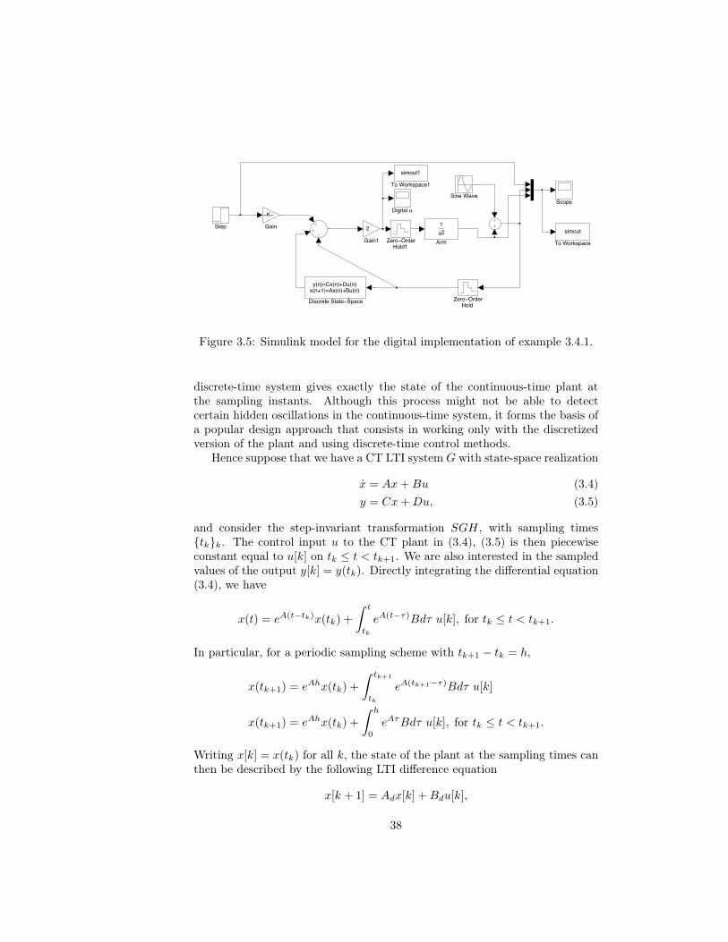
where uc[k] = uc(kh) and y[k] = y(kh) are the sampled values of the inputreference and (noise perturbed) plant output. A Simulink model of this im-plementation is shown on Fig. 3.5. As you can see on the right of Fig. 3.4,for a choice of sampling period h = 0.5 that is too large, there is a significantdeterioration of the output signal due to the presence of a clearly visible lowfrequency component.

This phenomenon is explained by the aliasing phenomenon, as discussedabove. We have ωs = 2π/h = 2π/0.5 ≈ 12.57 rad/s, and the measured signalhas a frequency 12 rad/s, well above the Nyquist frequency. After sampling,we then have the creation of a low frequency component with the frequency12.57 − ωs = 0.57 rad/s, in other word with a period of approximately 11 s,which is the signal observed on the right of Fig. 3.4.

Exercise 4. Derive (3.3).

Step-Invariant discretization of linear state-space systems

In this section, we consider a state-space realization of an LTI plant insteadof working in the frequency domain as in the previous paragraph. It turnsout that the step-invariant discretization of such as plant can be describedexactly (i.e., without approximation error) by a discrete-time LTI system. This

36

K Plant Py

ucu

0 5 10 150

0.2

0.4

0.6

0.8

1

1.2

1.4

time

uc(t)y(t)

Figure 3.3: Feedback control system and step response for example 3.4.1 withJ = k = ω0 = 1.

0 5 10 15−0.2

0

0.2

0.4

0.6

0.8

1

1.2

input uc

measured outputplant output

0 5 10 15−0.6

−0.4

−0.2

0

0.2

0.4

0.6

0.8

time

0 5 10 15 20 25−0.2

0

0.2

0.4

0.6

0.8

1

1.2

1.4

time

input uc

measured outputplant output

0 5 10 15 20 25−0.4

−0.3

−0.2

−0.1

0

0.1

0.2

0.3

0.4

0.5

0.6

time

Figure 3.4: Effect of a periodic perturbation on the continuous-time design(left) and discretized design with sampling period 0.5 (right), for example 3.4.1.The bottom row shows the analog input u to the plant. The analog controllerprovides a significant action, whereas the digital controller does not seem to beable to detect the high-frequency measurement noise.

37

Zero OrderHold1

Zero OrderHold

To Workspace1

simout1

To Workspace

simoutStep

Sine WaveScope

Gain1

2Gain

K

Discrete State Space

y(n)=Cx(n)+Du(n)x(n+1)=Ax(n)+Bu(n)

Digital u

Arm

1s 2

Figure 3.5: Simulink model for the digital implementation of example 3.4.1.

discrete-time system gives exactly the state of the continuous-time plant atthe sampling instants. Although this process might not be able to detectcertain hidden oscillations in the continuous-time system, it forms the basis ofa popular design approach that consists in working only with the discretizedversion of the plant and using discrete-time control methods.

Hence suppose that we have a CT LTI system G with state-space realization

x = Ax+Bu (3.4)y = Cx+Du, (3.5)

and consider the step-invariant transformation SGH, with sampling times{tk}k. The control input u to the CT plant in (3.4), (3.5) is then piecewiseconstant equal to u[k] on tk ≤ t < tk+1. We are also interested in the sampledvalues of the output y[k] = y(tk). Directly integrating the differential equation(3.4), we have

x(t) = eA(t−tk)x(tk) +

�t

tk

eA(t−τ)Bdτ u[k], for tk ≤ t < tk+1.

In particular, for a periodic sampling scheme with tk+1 − tk = h,

x(tk+1) = eAhx(tk) +

�tk+1

tk

eA(tk+1−τ)Bdτ u[k]

x(tk+1) = eAhx(tk) +

�h

0eAτBdτ u[k], for tk ≤ t < tk+1.

Writing x[k] = x(tk) for all k, the state of the plant at the sampling times canthen be described by the following LTI difference equation

x[k + 1] = Adx[k] +Bdu[k],

38

with Ad = eAh and Bd =�h

0 eAτBdτ . Note that this exact discretization couldhave been used in example 3.4.1 instead of the approximate Euler scheme.In summary, with periodic sampling the plant is represented at the samplinginstants by the DT LTI system

x[k + 1] = Adx[k] +Bdu[k]

y[k] = Cx[k] +Du[k].

Remark. The matrix exponential, necessary to compute Ad, can be computedusing the MATLAB expm funtion. There are various ways of computing Bd.The most straightforward is to simply use the MATLAB function c2d whichperforms the step-invariant discretization with a sampling period value pro-vided by the user. Actually this function also provides other types of discretiza-tion, including plant discretization using FOH, and other types of discretizationfor continuous-time controllers (rather than controlled plants), discussed laterin this chapter.

A few identities are sometimes useful for computations or in proofs. Firstdefine

Ψ =

�h

0eAτdτ = Ih+

Ah2

2!+ . . .

Then we have Bd = ΨB, and Ad = I + AΨ. Moreover, we have the followingresult.

Lemma 3.4.2. Let A11 and A22 be square matrices, and define for t ≥ 0

exp

�t

�A11 A12

0 A22

��=

�F11(t) F12(t)

0 F22(t)

�. (3.6)

Then F11(t) = etA11 , F22 = etA22 , and

F12(t) =

�t

0e(t−τ)A11A12e

τA22dτ.

Using this lemma, one can compute Ad and Bd using only the matrix ex-ponential function for example, by taking t = h,A11 = A,A22 = 0, A12 = B,so that F11(h) = Ad and F12(h) = Bd.

Proof. The expressions for F11 and F22 are immediate since the matrices areblock triangular. To obtain F12, differentiate (3.6)

d

dt

�F11(t) F12(t)

0 F22(t)

�=

�A11 A12

0 A22

� �F11(t) F12(t)

0 F22(t)

�,

henced

dtF12(t) = A11F12(t) +A12F22(t).

We then solve this differential equation, using the facts F22(t) = etA22 andF12(0) = 0.

39

Discretization of Linear Stochastic Differential Equations

Mathematically, it is also impossible to sample directly a signal containingwhite noise, a popular form of disturbance in control and signal processingmodels. Formally, the autocovariance function of a continuous-time zero-mean,vector valued white noise process w(t) is a Dirac delta

E[w(t)w(t�)T ] = r(t− t�) = W δ(t− t�). (3.7)

In other words, the values of the signal at different times are uncorrelated, asfor discrete-time white noise. The power spectral density of w is defined as theFourier transform of the autocovariance function

φw(ω) =

� ∞

−∞

r(t)e−iωtdt =

� ∞

−∞

W δ(t)e−iωtdt = W,

hence W is called the power spectral density matrix of w. The frequency con-tent of w is flat with infinite bandwidth. Hence intuitively, according to thefrequency folding phenomenon illustrated in lemma 3.2.1, the resulting sampledsignal would have infinite power in the finite band (−ωN ,ωN ).

Mathematically rigorous theories for manipulating models involving whitenoise are usually developed by working instead with an integral version of whitenoise

B(t) =

�t

0w(s)ds, B(0) = 0.

One can then use this theory to justify a posteriori the engineering formulasoften formulated in terms of Dirac deltas such as (3.7) 5. The stochastic processB has zero mean value and its increments I(s, t) = B(t) − B(s) over disjointintervals are uncorrelated with covariance

E[(B(t)−B(s))(B(t)−B(s))T ] = |t− s|W.

For this reason, Wdt is sometimes called the incremental covariance matrix ofthe process B. The stochastic process B is called Brownian motion or Wienerprocess if in addition the increments have a Gaussian distribution. Note thatin this case the increments over disjoint intervals are in fact independent, as aconsequence of a well-known property of Gaussian random variables. We thencalled the corresponding white noise (zero-mean) Gaussian white noise.

Gaussian white noise (or equivalently the Wiener process) is the most im-portant stochastic processes for control system applications, in particular be-cause one can derive from it other noise processes with a desired spectral densityby using it as an input to an appropriate filter (this is a consequence of spec-tral factorization, which you might want to review). The advantage of thisapproach is that we can then only work with white noise and take advantageof the uncorrelated samples property to simplify computations.

5Another approach would be to work with white noise rigorously using the theory ofdistributions, but in general this is unnecessarily complicated and it is just simpler to useintegrated signals.

40

Continuous-time processes with stochastic disturbances are thus often de-scribed by a stochastic differential equation, e.g. of linear form

dx

dt= Ax+Bu+ w(t),

where w is a zero-mean white noise process with power spectral density matrixW , which moreover we will assume to be Gaussian. Mathematically, it is thenmore rigorous to write this equation in the incremental form

dx = (Ax+Bu)dt+ dB1(t), (3.8)

where B1 is a Wiener process with incremental covariance R1dt. This equationjust means the integral form

x(t) = x(0) +

�t

0(Ax+Bu)dt+

�t

0dB1(t),

where the last term is called a stochastic integral and can be rigorously defined.Similarly, white noise can be used to model measurement noise. In this case,instead of the form

y = (Cx+Du) + v,

where y is the measured signal and v is white Gaussian noise with powerspectral density matrix V , we work with the integrated signal z(t) =

�t

0 y(s)ds,so that we can write again more rigorously

dz = (Cx+Du)dt+ dB2(t), (3.9)

where B2 is a Wiener process with incremental covariance R2dt. It is assumedthat the processes B2 and B2 are independent.

Now assume that the process is sampled at discrete times {tk}k, and thatwe want as in the deterministic case to relate the values of x and z at thesampling times. Integrating (3.8) and denoting hk = tk+1 − tk, we get6

x(tk+1) = eAhkx(tk) +

�tk+1

tk

eA(tk+1−τ)Gudτ +

�tk+1

tk

eA(tk+1−τ)dB1(τ).

Assuming a fixed value hk = h for the intersample intervals and a ZOH, we get

x[k + 1] = Adx[k] +Bdu[k] + w[k],

where Ad and Bd are obtained as in the deterministic case, and the sequence{w[k]}k is a random sequence. This random sequence has the following prop-erties, which come from the construction of stochastic integrals. First, therandom variables w[k] have zero mean

E(w[k]) = E��

tk+1

tk

eA(tk+1−τ)dB1(τ)

�= 0,

6This can be admitted formally, by analogy with the deterministic case.

41

and a Gaussian distribution, which are general properties of these stochasticintegrals. Their variance is equal to

E(w[k]w[k]T ) = E��

tk+1

tk

eA(tk+1−τ)dB1(τ)

�tk+1

tk

dBT

1 (τ�)eA

T (tk+1−τ�)

�

=

�tk+1

tk

�tk+1

tk

eA(tk+1−τ)W δ(τ − τ �)eAT (tk+1−τ

�)dτdτ �

=

�tk+1

tk

eA(tk+1−τ)WeAT (tk+1−τ)dτ. (3.10)

Here we have used the formal manipulations of Dirac deltas, but this formulais in fact a consequence of the Ito isometry. Finally, essentially by the inde-pendent increment property of the Brownian motion, we have that variablesw[k] and w[k�] for k �= k� are uncorrelated (or independent here since they areGaussian)

E(w[k]w[k�]) = 0, k �= k�.

In other work, {w[k]}k is a discrete-time white Gaussian noise sequence withcovariance matrix Wd given by (3.10), which we can rewrite

Wd =

�h

0eAtWeA

Ttdt,

by the change of variables u = tk+1 − τ . Note in particular that

Wd ≈ Wh

for h small.Let us now consider the sampling of the stochastic measurement process

(3.9). Note first that we have

y[k + 1] = z(tk+1)− z(tk) =

�tk+1

tk

y(τ)dτ, (3.11)

which corresponds physically to the fact mentioned earlier that the randomsignal y containing high-frequency noise is not sampled directly but first inte-grated7. Thus we have

y[k + 1] = z(tk+1)− z(tk)

=

��tk+1

tk

CeA(t−tk)dt

�x[k] +

��tk+1

tk

�t

tk

CeA(t−τ)dτdtB +Dhk

�u[k] + v[k],

=:Cdx[k] +Ddu[k] + v[k],

7Other forms of analog pre-filtering are possible and must be accounted for explicitly,by including a state-space model of the AAF filter. The simple integrate and reset filter (oraverage and reset) is the most commonly discussed in the literature on stochastic systemshowever.

42

where

v[k] = +

�tk+1

tk

�t

tk

CeF (t−τ)dB1(τ)dt+B2(tk+1)−B2(tk).

Note first that the expressions for Cd, Dd can be rewritten

Cd =

�h

0CeAtdt

Dd =

�tk+1

tk

�tk+1

τ

CeA(t−τ)dtdτB +Dh

=

�tk+1

tk

��tk+1−τ

0CeAsds

�dτB +Dh

=:

�tk+1

tk

θ(tk+1 − τ)dτB +Dh

=

�h

0θ(u)duB +Dh.

Note the definition θ(t) := C�t

0 eAsds. Similarly for v[k] we have

v[k] =

�tk+1

tk

θ(tk+1 − τ)dB1(τ) +B2(tk+1)−B2(tk).

Again {v[k]} is a sequence of Gaussian, zero-mean and independent randomvariables, i.e., discrete-time Gaussian white noise. We can also immediatelycompute [Åst06, p.83]

E(v[k]v[k]T ) =�

tk+1

tk

θ(tk+1 − τ)Wθ(tk+1 − τ)dτ + V h

=

�h

0θ(s)WθT (s)ds+ V h =: Vd

E(w[k]v[k�]T ) = δ[k − k�]

�h

0eAsWθT (s)ds =: δ[k − k�]Sd.

Note in particular that the discrete samples w[k] and v[k] are not independenteven if B1 and B2 are independent Wiener processes!

In summary, we obtain after integration of the output and sampling astochastic difference equation of the form

x[k + 1] = Adx[k] +Bdu[k] + w[k] (3.12)y[k + 1] = Cdx[k] +Ddu[k] + v[k] (3.13)

where the covariance matrix of the discrete-time noise can also be expressed as

E��

w[k]v[k]

� �w[k]v[k]

�T�=

�Wd Sd

ST

dVd

�=

�h

0eAt

�W 00 V

�eA

Ttdt, (3.14)

43

withA =

�A 0C 0

�⇒ eAt =

�eAt 0

C�t

0 eAτdτ I

�,

using Lemma 3.4.2.Remark. Some authors assume that the measurements are of the averagingform

y[k + 1] =1

h

�tk+1

tk

y(t)dt,

instead of (3.11), see e.g. [GYAC10]. Then θ(t) ≈ C for t close to zero, insteadof θ(t) ≈ Ct as t → 0 here. This results in a covariance matrix where (3.14)should be multiplied on the left and right by blkdiag(I, I/h). As a consequenceof this choice however, the variance of the discrete-time measurement noisev[k] diverges as h → 0, and one should work with power spectral densities[GYAC10].Remark. Note that in (3.13), there is a delay in the measurement, in con-trast to the standard form of difference equations. Such a discrete-time de-lay is theoretically not problematic, since we can redefine the state as x[k] =[x[k]T , x[k − 1]T ]T and the measurement as y[k] =

�0 Cd

�x[k]. Doubling the

dimension of the state space has computational consequences however.

Nonlinear Systems

Poles and Zeros of Linear Sampled-Data Systems

Incremental Models

Choice of Sampling Frequency

Generalized Sample and Hold Functions

3.5 Discretization of Continuous-Time Controllers

3.6 Quantization Issues

3.7 Complements on Modern Sampling Theory andReconstruction

44