frequency domain analysis of sampled-data control systems
TRANSCRIPT

Frequency Domain Analysis ofSampled-Data Control Systems
Julio Hernan Braslavsky
A thesis submitted in partial fulfilment ofthe requirements for the degree of
Doctor of Philosophy
THE DEPARTMENT OFELECTRICAL AND COMPUTER ENGINEERING
THE UNIVERSITY OF NEWCASTLENEW SOUTH WALES, 2308
AUSTRALIA
October 1995

Copyright c©1995 by Julio H. BraslavskyDepartment of Electrical and Computer EngineeringThe University of NewcastleNSW 2308 Australia
Revised April 1, 1996.
ISBN 7259 0905 6
Frequency Domain Analysis of Sampled-data Control SystemsBraslavsky, Julio Hernan - The University of Newcastle.Thesis - With index, references.Subject headings: Control systems analysis, sampled-data systems, discrete-time systems, frequency response.
This thesis was typeset by the author on a DEC Station using LATEX 2.09 +NFSS and Emacs. Typeset chapters where translated into PostScript files us-ing dvips. The typeface used for the main text is Concrete Roman, designedby Donald Knuth, and the mathematics font is Euler, designed by HermannZapf.
Printed in Australia by Lloyd Scott Document Production Services.

I hereby certify that the work embodied in this thesis is the re-sult of original research and has not been submitted for a higherdegree to any other University or Institution.
Julio H. Braslavsky


Acknowledgments
As somebody1 once said: “These summer days go very slow, but — let me tellyou, sweetheart — the years . . . fly by.”. And so went my years of postgrad stu-dent at the bushy campus of the University of Newcastle. Today, this period isalmost at its end, and the time of looking back has come. I’m indebted to manypeople for making this an enriching and unforgettable experience. First of all,I’d like to thank my supervisor, Rick Middleton. To work with him has been areal pleasure to me, with heaps of fun and excitement. Rick has oriented andsupported me with promptness and care, and has always been patient and en-couraging in times of difficulties. Above all, he made me feel a mate, whichI appreciate from my heart. My deep gratitude goes also to Jim Freudenberg.His dropping in Newcastle initiated the project that made this thesis possible. Ilearned many things from Jim, who has always been generous and patient in let-ting me grasp them. I was certainly lucky in having such a fine duo in the sameteam, of which I’m very proud to be part.
Thanks go also to Marcelo Laca, George Willis, and Brailey Sims. These guysendured with grace my visits to the Math Department, and deciphered the gib-berish I brought into well-formulated questions. I truly enjoyed the sessions of“amplification of doubts” spent with Marcelo in some lazy afternoons. Manytimes, I walked back the hill with some precious answers too.
The postgrads and post-postgrads of the EF Building have been an invaluablesupport day in, day out, during all these years. Special thanks to Juan, SingKiong, Gjerrit, Huai Zhong, Yash, Guillermo, Dragana, Misko, Lin, Bhujanga,Kim, Peng, Teresa, Brett, Steve, Jovica, Yuming, Ross, Jing Qiong, and Jaehoon.Very special thanks go to Gjerrit, a hero that proofread the thing and — at leastin compensation — enjoyed finding mistakes in my proofs2. Without the magicpowers of the wizard Huai Zhong — and, at the beginning of times, MichaelLund — working in front of the screen would have been a real pain. Thanks tothem for this.
Finally, my dearest thanks to people in this unique Department: Graham, Car-los, Minyue, Stefan, Hernan, Peter, Andrew S., Fernando, Andrew A., Marcia,Dianne, Denise, Roslyn and Vilma. You made me love this place. I take you all inmy heart3.
1Frank — Richard Harris in the excellent movie Wrestling Ernest Hemingway (1993).2I forgive him; he also introduced me to the enchanting art of boomeranging.3Hopefully, some of them will also remember a fisherman that once put a handkerchief in his
mouth.

Agradecimientos
Mi mas calido reconocimiento es para quienes estuvieron siempre conmigo— aun sin estar — y ası hicieron esta experiencia posible, con apoyo constantey, sobre todo, con mucho mucho carino. Para mi mama y mi papa, Marıa Elenay Julio, que incansablemente estimularon mis iniciativas, a pesar de que muchasde ellas significaran largos anos de vivir a la distancia, lejos del pago familiartan querido. A ellos que con su ejemplo me ensenaron que toda experiencia valemucho mas si es compartida.
Para Martha y Rafael, que fueron una conexion constante con la matria rosa-rina. Un afecto que no se puede medir en las toneladas de diarios, revistas ycompacts, que se la pasaron en gruesos sobres marrones haciendo el transpolarpara aterrizar en Newcastle.
Para los entranables amigos y companeros de estudio y de trabajo: German,Sergio, Monina, Juan Carlos, Roberto Riva4; de los que me lleve una parte en elcorazon5 y a los que volvere. Para Roberto Gonzalez y Ricardo Aimaretti, conquienes, alla lejos y hace tiempo, empezo toda esta historia.
Para Carmen, que a fuerza de carino hizo de Newcastle nuestro lugar.Y especialmente, para Marimar, mi companera y amada. Para ella tambien,
mi cancion es otra.
4Bueh, este de trabajo mucho no. . . pero buena joda.5Juan Carlos caso extremo: se vino entero.

A Marıa Elena y Julio Oscar.A Encarnacion.


Contents
Abstract 1
1 Introduction 31.1 Recent Developments in Sampled-data Systems . . . . . . . . . . . 41.2 Contributions of this Thesis . . . . . . . . . . . . . . . . . . . . . . . 7
2 Preliminaries 112.1 Analog and Discrete Signals . . . . . . . . . . . . . . . . . . . . . . . 11
2.1.1 Signal Spaces . . . . . . . . . . . . . . . . . . . . . . . . . . . 112.1.2 Samplers and Holds . . . . . . . . . . . . . . . . . . . . . . . 122.1.3 A Key Sampling Formula . . . . . . . . . . . . . . . . . . . . 15
2.2 Hybrid Systems . . . . . . . . . . . . . . . . . . . . . . . . . . . . . . 172.2.1 Basic Feedback Configuration . . . . . . . . . . . . . . . . . . 172.2.2 Non-pathological Sampling and Internal Stability . . . . . . 20
2.3 Summary . . . . . . . . . . . . . . . . . . . . . . . . . . . . . . . . . . 21
3 Generalized Sampled-data Hold Functions 233.1 Frequency Response of Generalized Sampled-data Holds . . . . . . 24
3.1.1 Norms and the Frequency Response of a GSHF . . . . . . . 253.1.2 GSHF Frequency Responses from Boundary Values . . . . . 273.1.3 Two Simple Classes of GSHFs . . . . . . . . . . . . . . . . . . 28
3.2 Distribution of Zeros of GSHFs . . . . . . . . . . . . . . . . . . . . . 303.2.1 Zeros of PC and FDLTI GSHFs . . . . . . . . . . . . . . . . . 313.2.2 GSHFs with all Zeros on the jω-axis . . . . . . . . . . . . . . 323.2.3 Example: Zeros of a FDLTI GSHF . . . . . . . . . . . . . . . 36
3.3 Integral Relations . . . . . . . . . . . . . . . . . . . . . . . . . . . . . 383.3.1 Poisson Integral for GSHFs . . . . . . . . . . . . . . . . . . . 403.3.2 Middleton Integral for GSHFs . . . . . . . . . . . . . . . . . 423.3.3 Example: Tradeoffs in H(jω) . . . . . . . . . . . . . . . . . . 46
3.4 Summary . . . . . . . . . . . . . . . . . . . . . . . . . . . . . . . . . . 46
4 Frequency Response and Performance Limitations 494.1 Frequency Response of a Sampled-data System . . . . . . . . . . . . 504.2 Interpolation Constraints . . . . . . . . . . . . . . . . . . . . . . . . . 554.3 Hybrid Disturbance Rejection Properties . . . . . . . . . . . . . . . . 614.4 Integral Relations . . . . . . . . . . . . . . . . . . . . . . . . . . . . . 68
4.4.1 Notation . . . . . . . . . . . . . . . . . . . . . . . . . . . . . . 694.4.2 Poisson Sensitivity Integral . . . . . . . . . . . . . . . . . . . 70

x Contents
4.4.3 Poisson Complementary Sensitivity Integral . . . . . . . . . 734.4.4 Poisson Harmonic Response Integral . . . . . . . . . . . . . 754.4.5 Bode Sensitivity Integral . . . . . . . . . . . . . . . . . . . . . 774.4.6 Middleton Complementary Sensitivity Integral . . . . . . . 77
4.5 Summary . . . . . . . . . . . . . . . . . . . . . . . . . . . . . . . . . . 80
5 Sensitivity Operators on L2 815.1 A Frequency-domain Lifting . . . . . . . . . . . . . . . . . . . . . . . 825.2 L2-induced Norms and Frequency-gains . . . . . . . . . . . . . . . . 85
5.2.1 Sensitivity Operators . . . . . . . . . . . . . . . . . . . . . . . 855.2.2 Numerical Implementation . . . . . . . . . . . . . . . . . . . 93
5.3 Summary . . . . . . . . . . . . . . . . . . . . . . . . . . . . . . . . . . 99
6 Stability Robustness 1016.1 Multiplicative Perturbation . . . . . . . . . . . . . . . . . . . . . . . 1026.2 Divisive Perturbation . . . . . . . . . . . . . . . . . . . . . . . . . . . 1106.3 Summary . . . . . . . . . . . . . . . . . . . . . . . . . . . . . . . . . . 113
7 An Application: Design Implications of Discrete Zero-placement 1157.1 Discrete Zero-placement and ORHP Zeros of GSHFs . . . . . . . . . 1177.2 Gedanken Experiment No. 1: Analog Performance . . . . . . . . . . 1207.3 Gedanken Experiment No. 2: Discrete Response . . . . . . . . . . . 122
7.3.1 Formulation of Gedanken Experiment No. 2 . . . . . . . . . 1227.3.2 Interpolation Constraints and an Integral Relation . . . . . . 1247.3.3 Result of Gedanken Experiment No. 2 . . . . . . . . . . . . . 1267.3.4 Example: Robustness of Zero-placement . . . . . . . . . . . 129
7.4 Summary . . . . . . . . . . . . . . . . . . . . . . . . . . . . . . . . . . 132
8 Conclusions 133
A Proofs of Some Results in the Chapters 137A.1 Proofs for Chapter 2 . . . . . . . . . . . . . . . . . . . . . . . . . . . . 137A.2 Proofs for Chapter 3 . . . . . . . . . . . . . . . . . . . . . . . . . . . . 139A.3 Proofs for Chapter 4 . . . . . . . . . . . . . . . . . . . . . . . . . . . . 141
A.3.1 Proof of Lemma 4.1.2 . . . . . . . . . . . . . . . . . . . . . . . 141A.3.2 Proof of Theorem 4.4.11 . . . . . . . . . . . . . . . . . . . . . 144
A.4 Proofs for Chapter 5 . . . . . . . . . . . . . . . . . . . . . . . . . . . . 147A.5 Proofs for Chapter 6 . . . . . . . . . . . . . . . . . . . . . . . . . . . . 148
B Order and Type of an Entire Function 151
C Discrete Sensitivity Integrals 153
Bibliography 157
Notation 165

Abstract
This thesis is aimed at analysis of sampled-data feedback systems. Our approachis in the frequency-domain, and stresses the study of sensitivity and complemen-tary sensitivity operators. Frequency-domain methods have proven very success-ful in the analysis and design of linear time-invariant control systems, for whichthe importance and utility of sensitivity operators is well-recognized. The exten-sion of these methods to sampled-data systems, however, is not straightforward,since they are inherently time-varying due to the intrinsic sample and hold oper-ations.
In this thesis we present a systematic frequency-domain framework to de-scribe sampled-data systems considering full-time information. Using this frame-work, we develop a theory of design limitations for sampled-data systems. Thistheory allows us to quantify the essential constraints in design imposed by in-herent open-loop characteristics of the analog plant. Our results show that: (i)sampled-data systems inherit the difficulty imposed upon analog feedback de-sign by the plant’s non-minimum phase zeros, unstable poles, and time-delays,independently of the type of hold used; (ii) sampled-data systems are subject toadditional design limitations imposed by potential non-minimum phase zeros ofthe hold device; and (iii) sampled-data systems, unlike analog systems, are sub-ject to limits upon the ability of high compensator gain to achieve disturbancerejection. As an application, we quantitatively analyze the sensitivity and robust-ness characteristics of digital control schemes that rely on the use of generalizedsampled-data hold functions, whose frequency-response properties we describein detail.
In addition, we derive closed-form expressions to compute the L2-inducednorms of the sampled-data sensitivity and complementary sensitivity operators.These expressions are important both in analysis and design, particularly whenuncertainty in the model of the plant is considered. Our methods provide someinteresting interpretations in terms of signal spaces, and admit straightforwardimplementation in a numerically reliable fashion.


1Introduction
This thesis deals with frequency-domain properties and essential design limita-tions in linear sampled-data feedback control systems.
A sampled-data system combines both continuous and discrete-time dynamicsubsystems. Because of this inherent mixture of time domains, we shall also referto a sampled-data system as a hybrid system, understanding both terms as syn-onyms. A typical hybrid feedback control configuration is shown in Figure 1.1.Although the plant is usually a continuous-time, or analog, system, the controlleris a discrete-time device in most practical applications. This is mainly due to thenumerous advantages that digital equipments offer over their analog counter-parts. With the great advances in computer technology, today digital controllersare more compact, reliable, flexible and often less expensive than analog ones.
There is a fundamental operational difference between digital and analog con-trollers: the digital system acts on samples of the measured plant output ratherthan on the continuous-time signal. A practical implication of this difference isthat a digital controller requires special interfaces that link it to the analog world.
?ib
bbaa qiib
6
-
--- -
?
- ?-+
−
Referenceinput
noiseMeasurement
Output
Digital Controller
Plant
+
+ +
Outputdisturbances
+
DigitalcomputerA-D
D-A
Figure 1.1: Typical sampled-data feedback configuration.
A digital controller can be idealized as consisting of three main elements: theanalog-to-digital (A-D) interface, the digital computer, and the digital-to-analog(D-A) interface. The A-D interface, or sampler, acts on a physical variable, nor-mally an electric voltage, and converts it into a sequence of binary numbers,which represent the values of the variable at the sampling instants. These num-bers are then processed by the digital computer, which generates a new sequence

4 1. Introduction
of binary numbers that correspond to the discrete control signal. This control sig-nal is finally converted into an analog voltage by the D-A interface, also calledthe hold device.
The digital computer implements the control algorithm as a set of differenceequations, which represent a dynamic system in the discrete-time domain. Weshall refer to this system as the discrete controller. In general, the discrete controllerwill include nonlinearities and varying parameters in it; our discussion here isrestricted to linear time-invariant controllers, which nevertheless constitute anuseful and important case in analysis and design.
Essentially, two classic approaches are taken in engineering practice for thedesign of a discrete controller. The first technique, referred to as emulation [Franklinet al., 1990], is the most widely applied in industry. Emulation consists in firstdesigning an analog controller such that the closed-loop system has satisfactoryproperties, and then translating the analog design into a discrete one using asuitable discretization method (see Keller and Anderson [1992] for a recent ap-proach). This technique has the advantage that the synthesis is done in continuous-time, where the design goals are typically specified, and where most of the de-signer’s experience and intuition resides. Also, the system’s analog performancewill in general be recovered for fast sampling. Yet, the hybrid performance cannotbe expected to be better than the analog, and there may be a serious degradationif the sampling is not sufficiently fast. This is an important drawback, since thesampling rate is a critical constraint in many applications.
The second traditional technique consists in discretizing the plant and per-forming a discrete design. The main benefit of this approach is that the synthesisprocedure is again simplified, since the discretized plant is linear time-invariant(LTI) in the discrete-time domain. However, a serious limitation of discrete de-sign is that it is generally difficult to translate the analog specifications into dis-crete. Furthermore, the simple models obtained by discretization fail to representthe full response of the system, since intersample behavior is inherently lost or hid-den1.
In particular, neither of these approaches offers an adequate framework foranalysis of the continuous-time time-varying hybrid system. Emulation is purelya method of synthesis, whereas discrete design gives a partial answer, since onlythe sampled behavior can be studied in the discretized model. On the other hand,the analysis of the hybrid system requires the consideration of both sampled andintersample behavior. This is crucial especially when considering robustness andsensitivity properties of the system, since analog uncertainties, disturbances andnoise are frequently the issues of practical significance.
1.1 Recent Developments in Sampled-data Systems
Naturally, in view of the technological appeal of digital implementations, sampled-data systems have been the subject of many research works in recent years. Two
1Some intersample information can still be handled in a discrete model by using the modified Z-transform introduced by Jury [1958]. However, this line of work seems to have been largely aban-doned.

1.1 Recent Developments in Sampled-data Systems 5
research directions in particular have generated much activity. First, various op-timal control problems have been stated and solved for hybrid systems usingframeworks that incorporate intersample behavior [e.g., Chen and Francis, 1991,Bamieh and Pearson, 1992, Dullerud and Francis, 1992, Tadmor, 1992, Kabambaand Hara, 1993, Bamieh et al., 1993]. Second, several researchers have exploredthe potential ability of nonstandard hold functions, periodic digital controllers,and multirate sampling to circumvent design limitations inherent to LTI sys-tems [e.g., Khargonekar et al., 1985, Kabamba, 1987, Francis and Georgiou, 1988,Hagiwara and Araki, 1988, Das and Rajagopalan, 1992, Yan et al., 1994]. Withinthese two research avenues, we shall restrict the discussion here to optimal H∞sampled-data control, and control techniques using generalized sampled-data holdfunctions (GSHFs).
The earliest efforts to extend H∞ control methods to sampled-data systemsfocused on the computation of the induced L2-norm. The L2-induced norm mea-sures the maximum gain of an operator acting on spaces of square integrable,or “finite energy”, signals. For a LTI system, the optimization of the L2-inducednorm is equivalent to the minimization of the H∞-norm of its transfer matrix.This is not trivial to extend to sampled-data systems, since they are time-varyingdue to the presence of the sampler, and hence we cannot describe their input-output behavior with ordinary transfer matrices. Therefore, special procedureshave been developed. For example, Thompson et al. [1983], and Thompson et al.[1986] provided the first bounds for the norm of open-loop hybrid systems usingconic sector techniques. Exact expressions of the L2-induced norms were lateron obtained by Chen and Francis [1990] via frequency-domain methods. In 1991,Leung et al. derived a formula for sampled-data feedback systems with band-limited signals.
In recent years, different general frameworks to handle intersample behaviorappeared on the scene, and led the way to the solution of certain hybrid optimalH∞ control problems2. These frameworks include lifting techniques [Bamieh et al.,1991, Toivonen, 1992, Bamieh and Pearson, 1992, Yamamoto, 1993, 1994], descrip-tor system techniques [Kabamba and Hara, 1993], and techniques based on linearsystems with jumps [Sun et al., 1993, Sivashankar and Khargonekar, 1994]. Morespecifically, the lifting technique consists on transforming the original sampled-data system into an equivalent LTI discrete-time system with infinite-dimensionalinput-output signal spaces. Then, the L2-induced norm of the sampled-data sys-tem is shown to be less than one if and only if the H∞-norm of this equivalentdiscrete system is less than one. In the descriptor system approach, on the otherhand, the system is represented by a hybrid state-space model, from which thedescriptor system is formulated. The solution of the H∞ sampled-data problemis then characterized by the solution of certain associated Hamiltonian equation.In contrast with these procedures, the theory of linear systems with jumps allowsa direct characterization of the problem in similar — although more involved —terms to those of standard LTIH∞-control problems, and leads to a pair of Riccatiequations. Despite the procedural differences in all these approaches, the results
2Yet, as pointed out by Glover [1995], practical design guidelines are still under development.

6 1. Introduction
obtained are mathematically equivalent.
On the other hand, new control schemes using GSHFs were introduced to ap-proach various problems that are insoluble with LTI control schemes. A GSHFreconstructs an analog signal from a discrete sequence of values, but instead ofholding these values constant along the sample period — as it is the case of a clas-sic zero-order hold (ZOH) — a GSHF scales a fixed suitable waveform. In particu-lar, by selecting this waveform it is possible to assign the zeros of the discretizedplant, and hence, e.g., convert a non-minimum phase (NMP) analog plant intoa minimum phase discrete plant [Bai and Dasgupta, 1990]. This is the key tech-nique of several applications of GSHFs. For example, Kabamba [1987] obtainedsimultaneous pole-assignment of an arbitrary finite number of plants using a sin-gle GSHF; and Yan et al. [1994] proposed the combination of a discrete controllerwith a GSHF to achieve arbitrary gain-margin improvement of continuous-timeNMP linear systems. Other applications of GSHFs include decoupling, exactmodel-matching, and exact discrete loop transfer recovery of NMP plants [Liuet al., 1992, Paraskevopoulos and Arvanitis, 1994, Er and Anderson, 1994].
Besides the benefits offered by GSHFs, some authors have pointed out theexistence of intersample difficulties and serious robustness and sensitivity prob-lems associated with the use of these devices [Araki, 1993, Feuer and Goodwin,1994, Zhang and Zhang, 1994]. For example, Feuer and Goodwin [1994] haveargued that GSHF control relies on the generation of high-frequency harmonics,which tend to make the system more sensitive to high-frequency plant uncer-tainty, disturbances and noise. As a consequence, the potential utility of GSHFsin overcoming LTI design limitations seems still to be a matter of debate.
Despite these advances in synthesis, there is as yet no well-developed the-ory of inherent design limitations for hybrid feedback systems. For analog feed-back systems, on the other hand, many results on design limitations are available.Bode first stated the sensitivity integral theorem in 1945, whose importance forfeedback control was emphasized by Horowitz [1963]. Later extensions were ob-tained by several researchers; of particular relevance to the present discussion arethe results of Freudenberg and Looze [1985] and Middleton [1991]. Briefly, thetheory describes how plant properties such as NMP zeros, unstable poles, andtime delays limit the achievable performance of a feedback system consisting ofa LTI plant and a continuous-time controller. These limitations manifest them-selves as tradeoffs between desirable system properties in different frequencyranges, and are expressed mathematically using Bode and Poisson integrals.
A parallel theory of inherent design limitations for purely discrete-time feed-back systems is also available [Sung and Hara, 1988, Middleton and Goodwin,1990, Mohtadi, 1990, Middleton, 1991]. Unfortunately, this theory is insufficientto describe fundamental limitations in hybrid systems. Indeed, discrete-time re-sults do not consider intersample behavior, and therefore do not tell us the wholestory (in particular, good sampled behavior is necessary but not sufficient forgood overall behavior). The development of an equivalent theory for sampled-data systems is one of the main goals of this thesis.

1.2 Contributions of this Thesis 7
1.2 Contributions of this Thesis
This thesis is aimed at analysis of sampled-data feedback systems. Our approachis in the frequency-domain, and stresses the study of sensitivity and complemen-tary sensitivity operators. Our main contributions may be summarized as fol-lows:
(i) We expound a systematic frequency-domain framework to describe sampled-data systems considering full-time information. This framework allows usto study important properties of the system in a way that appears to besimpler than in alternative state-space approaches. There are two reasonswhy we believe the frequency-domain approach to be simpler. First, thisfrequency-domain setting has better links with classical frequency-domainanalysis for analog control systems, in which a large heuristic knowledgeis available. Second, the mathematics involved seems easier to understandand relate to the original plant model.
(ii) We develop a theory of design limitations for sampled-data systems. Thistheory allows us to quantify the essential constraints imposed by NMP ze-ros of the hold function, and NMP zeros and unstable poles of the analogplant and discrete controller. As an application, we quantitatively analyzethe sensitivity and robustness properties of control schemes that rely onGSHF discrete zero-shifting capabilities.
(iii) We derive closed-form expressions to compute the L2-induced norms of thehybrid sensitivity and complementary sensitivity operators. These expres-sions have interesting interpretations in terms of signal spaces associatedwith the hold, the plant and the anti-aliasing filter. All our formulas admitstraightforward implementation in a numerically reliable fashion.
(iv) We study the frequency-domain properties of GSHFs, providing results thatdescribe in detail their zero-distribution, and some integral relations thattheir frequency response must satisfy. In particular, these results show thesource of some of the difficulties associated with the use of GSHFs.
The framework of (i), and the results of (iii) are valid for multiple-input multiple-output (MIMO) systems. The results in (ii) and (iv) are restricted to the single-input single-output (SISO) case. Due to the issue of directionality, the general-ization of these results to multivariable is difficult — for (ii) this is so even in theanalog case — and hence we have not pursued it here.
Many of the results referred to in (ii) have been developed in collaboration,and published in Freudenberg et al. [1995] and Freudenberg et al. [1994], withsignificant input from the first author. The results in (i) and (iii) have been par-tially communicated in Braslavsky et al. [1995b], while some of the results in (iv)will appear in Braslavsky et al. [1995a].
We now give an overview of the rest of the thesis.
Chapter 2: This chapter introduces most of our notation, main assumptions, andthe basic preliminary results upon which the rest of the chapters will be

8 1. Introduction
developed. Here, we define the mathematical representations of the A-Dand D-A interfaces, the sampler, and the hold device. A distinctive fea-ture of our approach is that the hold device is not restricted to the ZOH.Indeed, we shall consider that the hold is a GSHF of the type introduced byKabamba [1987], which will allows us to develop a comprehensive frame-work to study sampled-data systems. We also present in this chapter a basicbut key sampling formula concerning the Laplace transform of a sampledsignal. This relation will be the starting point of our discussion on the fre-quency response of hybrid systems in the following chapters. We concludewith a review of two important results concerning the closed-loop stabiliz-ability properties of sampled-data systems.
Chapter 3: The focus of this chapter is the frequency response of a GSHF. Asopposed to that of a ZOH, the frequency response of a GSHF may havelarge high-frequency peaks that compromise the robustness properties ofthe system. It is also known that GSHFs may have zeros off the jω-axis thatpose discrete stabilizability difficulties. In this chapter we go deeper intothe analysis of these issues by studying fundamental properties of the fre-quency response of GSHFs. Specifically, we describe their zero-distributionand the constraints that these zeros impose on the values on the jω-axis.One of the main results of this chapter is that GSHFs with “asymmetric”pulse response function will necessarily have zeros off the jω-axis.
Chapter 4: In this chapter, we study the frequency response of a sampled-datasystem, and develop a theory of design limitations wherein we considerthe response of the analog system output. To do this, we use the fact thatthe steady-state response of a hybrid feedback system to a sinusoidal inputconsists of a fundamental component at the frequency of the input togetherwith infinitely many harmonics, located at frequencies spaced integer mul-tiples of the sampling frequency away from the fundamental. This fact al-lows us to define fundamental sensitivity and complementary sensitivityfunctions that relate the fundamental component of the response to the in-put signal. These sensitivity and complementary sensitivity functions mustsatisfy integral relations analogous to the Bode and Poisson integrals forpurely analog systems. The relations show, for example, that design limi-tations due to NMP zeros of the analog plant constrain the response of thesampled-data feedback system regardless of whether the discretized systemis minimum phase, and independently of the choice of hold function.
Chapter 5: This chapter deals with the analysis and computation of the L2-inducednorm of operators in sampled-data systems. We first expound a frequency-domain lifting technique to derive “closed-form” expressions for the fre-quency gains of hybrid sensitivity operators in a MIMO setup. We showthat these frequency-gains can be characterized by the maximum eigen-value of certain finite-dimensional discrete transfer matrices; even in thecase of the sensitivity operator, which — since it is known to be non-compact— presents extra difficulties for the analysis. The L2-induced norm is then

1.2 Contributions of this Thesis 9
computed by searching the maximum of this eigenvalue over a finite rangeof frequencies. At the end of the chapter, we provide expressions fromwhich the generation of numerical algorithms to compute these norms isstraightforward.
Chapter 6: This chapter is about stability robustness of sampled-data systems.Dullerud and Glover [1993] have derived necessary and sufficient condi-tions for robust stability of hybrid systems against multiplicative perturba-tions in the analog system. These authors have used a frequency-domainformulation based on state-space lifting techniques. We show in this chap-ter that the same type of result may be obtained in a simpler way whenthe problem is directly formulated in the frequency-domain. We do thisby using the frequency-domain lifting framework introduced in Chapter 5.We also give both necessary conditions and sufficient conditions for robuststability as simple expressions that emphasize the role played by the fun-damental and harmonic sensitivity functions defined in Chapter 4. We con-clude the chapter by showing that the same framework may be used toapproach the problem of robust stability against divisive perturbations.
Chapter 7: As an application of the preceding results, in this chapter we studythe difficulties associated with the zero-shifting capabilities of GSHFs. ManyGSHF-based proposed schemes rely on zero-shifting, since this appears tocircumvent fundamental limitations imposed by analog NMP zeros. Weshow that if the plant has a NMP zero with significant phase lag within thedesired closed-loop bandwidth of the system, then zero-shifting will nec-essarily lead to serious robustness and sensitivity problems in both analogand discrete performances of the system.
Chapter 8: In this chapter we summarize the main results of the thesis, and givesome concluding remarks and directions for future research.


2Preliminaries
This chapter defines most of our notation, and introduces general assumptionsand preliminary results required in the sequel. We present a key formula concern-ing the Laplace transform of a sampled signal that will play an important role inthe rest of this thesis. This formula yields the well-known infinite summation ex-pression showing that the response of the discretized plant at a given frequencydepends upon that of the analog plant at infinitely many frequencies. We finishthe chapter reviewing the basic conditions for closed-loop stability of sampled-data systems; i.e., a non-pathological sampling assumption, and the closed-loopstability of the discretized system.
2.1 Analog and Discrete Signals
2.1.1 Signal Spaces
We start introducing some standard signal spaces. We denote the set of complexnumbers by C. The open and closed right halves of C are denoted by C+ and C+
respectively, and sometimes we shall use the acronyms ORHP and CRHP. Corre-spondingly, we denote by C− and C− the open and closed left halves of C, alsoreferred as OLHP and CLHP, respectively. We denote the set of real numbers byR, and by R+
0 we represent the set of non-negative real numbers, i.e., the segment[0,∞). The open and closed unit disks in C are denoted by D , z : |z| < 1 andD , z : |z| ≤ 1 respectively; we denote their complements by DC and D
C.
As usual, Lnp(R+0 ) denotes the space of Lebesgue measurable functions f from
R+0 to Rn that satisfy
‖f‖Lp ,(∫∞0
|f(t)|p dt
)1/p<∞ for 1 ≤ p <∞,
and‖f‖L∞ , ess sup
t∈R+0
|f(t)| <∞,where | · | denotes the Euclidean norm in Rn. We denote by Lnpe(R
+0 ) the extended
space of Lnp(R+0 ), i.e., the space of functions whose truncations to intervals [0, a)
are in Lnp(R+0 ) for any finite real number a.

12 2. Preliminaries
In a similar way, Ln2 denotes the space of functions F(jω) defined on jR withvalues over Cn and satisfying
‖F‖L2 ,(∫∞
−∞ |F(jω)|2 dω
)1/2<∞.
Here the Euclidean norm | · | is taken on Cn, i.e., |F| =√F∗F, where F∗ denotes the
complex conjugate transpose of F. In general, we shall denote the transpose of amatrixM byMT, and byM its conjugate.
In discrete-time we represent by `np the space of sequences u , uk∞k=−∞
valued in Cn and satisfying
‖u‖`p ,
( ∞∑k=−∞ |uk|
p
)1/p<∞ for 1 ≤ p <∞,
and‖u‖`∞ , sup
k
|uk| <∞.We shall dispense with the superscript n in the above notations whenever the
dimension of the spaces is clear from the context. We shall also omit the subindexthat indicates the spaces in the notation of norms ‖ · ‖ when they are clear fromthe context.
We shall represent linear dynamic systems as input-output operators actingon Lp spaces. If M is a linear operator defined by
M : Lp(R+0 )→ Lp(R
+0 )
: u 7→ y = Mu,
the Lp-induced norm of the operator M is defined as
‖M‖p , sup‖My‖Lp‖u‖Lp
: for u in Lp(R+0 ), and ‖u‖Lp 6= 0
.
A quick-reference list of the above notations may be found on page 165.
2.1.2 Samplers and Holds
As discussed in Chapter 1, the implementation of a controller for a continuous-time system by means of a digital device, such as a computer, implies the processof sampling and reconstruction of analog signals. By sampling, an analog signalis converted into a sequence of numbers that can then be digitally manipulated.The hold device performs the inverse operation, translating the output of thedigital controller into a continuous-time signal. We shall assume throughout thatnonlinearities associated with the process of discretization, such as finite memoryword-length, quantization, etc., have no significant effect on the sampled-datasystem.

2.1 Analog and Discrete Signals 13
We assume also that sampling is regular, i.e., if T is the sampling period, sam-pling is performed at instants t = kT , with k = 0,±1,±2, . . .. Associated with T ,we define the sampling frequency ωs = 2π/T . By ΩN we denote the Nyquist rangeof frequencies [−ωs/2,ωs/2].
We consider an idealized model of the sampler. If y is an analog signal definedon the time set R+
0 with values over Cn, we define the sampling operator withsampling period T , denoted by ST , as
ST y = yk∞k=−∞, (2.1)
where yk∞k=−∞ is the sequence representing the sampled signal, and yk = y(kT+)1.
Thus, the sampler is a linear, periodically time-varying operator. Note that thesampler operator may be unbounded in many standard signal spaces, as for ex-ample from Lp(R
+0 ) to `p when 1 ≤ p < ∞ Chen and Francis [1991]. Therefore,
we need to specify with some care the class of signals that are “sampleable”.A class of functions that guarantee that the sampling operator is well-defined
is the class of functions of bounded variation (BV). These functions will be requiredto define the hold devices we shall deal with, and to assure the validity of a sam-pling formula that will be the starting point of our approach to sampled-datasystems. The following definition is taken from Riesz and Sz.-Nagy [1990].
Definition 2.1.1 (Function of Bounded Variation)A function f defined over a real interval (a, b) is of BV if the following sum isbounded,
n∑k=1
|f(tk) − f(tk−1)| <∞, (2.2)
for every partition of the interval (a, b) into subintervals (tk, tk−1), where k =1, 2, . . . , n, and t0 = a, tn = b. The least upper bound of the sum in (2.2) is calledthe total variation of f in the interval (a, b).
A function of BV is not necessarily continuous, but it is differentiable almosteverywhere and its derivative is a function in L1(a, b) Rudin [1987]. Moreover,the limits f(t+) and f(t−) are well defined for every t in (a, b), which means thatf can have discontinuities of at most the finite-jump type.
The hold device that we shall consider is a GSHF a la Kabamba [1987], definedby the operation
u(t) = h(t− kT)uk, for kT ≤ t < (k+ 1)T, (2.3)
where uk∞k=−∞ is a discrete sequence, and h is a bounded function with support
on the interval [0, T). We consider the case in which the sequence uk∞k=−∞ takes
values in Rp, and so h takes values in Rp×p. We shall assume throughout that hsatisfies the following technical conditions.
1Here, y(kT±) denotes the right (left) limit of y(·) at t = kT , i.e.,
y(kT±) , limε↓0 f(kT ± ε), for ε > 0,
whenever the limit exists.

14 2. Preliminaries
Assumption 1The hold function h is a function of BV on [0, T).
As discussed in Middleton and Freudenberg [1995], we can associate a fre-quency response function to this hold device, defined by
H(s) =
∫T0
e−st h(t)dt. (2.4)
Since h is supported on a finite interval, it follows that H is an entire function,i.e., analytic at every s in C. For example, in the case of the ZOH we have thewell-known responseH(s) = (1− e−sT )/s. Frequency responses of other types ofholds will be studied in detail in Chapter 3.
We shall be particularly interested in the zeros of the response function H.These have transmission blocking properties, and may affect the stabilizability ofthe discretized system Middleton and Freudenberg [1995]. Furthermore, as weshall see in Chapter 4, they are an important factor in analysis of the achievableperformance of the sampled-data system.
Definition 2.1.2 (Zeros of the Hold Middleton and Freudenberg [1995])Consider a response function defined by (2.4) and suppose that det(H) is notidentically zero. Then the zeros of H are those values s in C for which H(s) hasless than full rank.
bb - -Huk u
Figure 2.1: Response of a GSHF.
The frequency response of the hold defined in (2.4) is useful to compute theLaplace transform of the output of the hold device (see Figure 2.1). As describedin Middleton and Freudenberg [1995], the i-th column of the frequency responsefunction (2.4) represents the Laplace transform of the output of the hold to anunitary pulse in the ith input. More generally, if Ud is the Z-transform of theinput sequence uk
∞k=−∞, then we have the following Astrom and Wittenmark
[1990].
Lemma 2.1.1Consider the hold defined by (2.3) and its associated frequency response (2.4).Then
U(s) = H(s)Ud(esT ).

2.1 Analog and Discrete Signals 15
GSHFs have been proposed as a more versatile alternative to the traditionalZOH [see for example Kabamba, 1987], and indeed, recent studies have shownthat if a solution to the sampled-data H∞ control problem exists, then it maybe realized by a LTI discrete controller and a GSHF Sun et al. [1993]. Neverthe-less, these devices certainly are much more complex to be implemented and —as some authors have suggested and we shall expand on — they may bring inserious intersample difficulties.
2.1.3 A Key Sampling Formula
Our approach to sampled-data systems is in the frequency-domain. We nowpresent a result that is essential to the understanding of the frequency-domainproperties of sampled-data systems and will play a central role throughout thefollowing chapters. Unfortunately, despite the fact that the result is well-knownand appears in many textbooks [e.g., Astrom and Wittenmark, 1990, Franklinet al., 1990, Kuo, 1992, Ogata, 1987], it is difficult to find in the literature a proofthat is rigorous and self-contained, and which clearly delineates the classes ofsignals to which it is applicable. Indeed, this fact has stimulated discussion in thepast [cf. Pierre and Kolb, 1964, Carroll and W.L. McDaniel, 1966, Phillips et al.,1966, 1968].
Let g be a function of BV in every finite interval of R+0 , and letG be its Laplace
transform,
G(s) =
∫∞0
e−st g(t)dt.
If σG is the abscissa of absolute — and uniform — convergence of G, we denoteby DG the strip
DG , s = x+ jy,with x > σG and y inΩN.
Given a sequence gk∞k=0, we introduce the Z-transform, Gd = Zgk, defined
by
Gd(z) =
∞∑k=0
gkz−k. (2.5)
For a continuous-time signal g defined on R+0 , and g(t) = 0 for t < 0, we define
the Z-transform as the transformation of its sampled version,
Gd(z) = ZST g
=
∞∑k=0
g(kT+) z−k.
Then we have the following lemma.
Lemma 2.1.2If g is a function of BV in every finite interval of R+
0 , then for every s in DG
Gd(esT ) =
g(0+)
2+
∞∑k=1
g(kT+) − g(kT−)
2e−skT +
1
T
∞∑n=−∞G(s+ jnωs). (2.6)
16 2. Preliminaries
Proof: See Appendix A, §A.1.
Lemma 2.1.2 shows the well-known fact that the frequency response of a sam-pled signal is built upon the superposition of infinitely many copies of the orig-inal frequency response of the signal. If the signal has finite discontinuities atthe sampling instants, then correction terms of half of the jumps at the corre-sponding sampling instants have to be included — cf. the property of the Laplaceand Fourier inverse transforms which converge to the average of the limits of thefunction from left and right at a jump discontinuity. In particular, (2.6) is closelyrelated to an important identity in Fourier analysis known as the Poisson Summa-tion Formula2. See further remarks in Appendix A, §A.1.
Moreover, Lemma 2.1.2 clearly de-
?c b b c- -
u yF
yd
ST
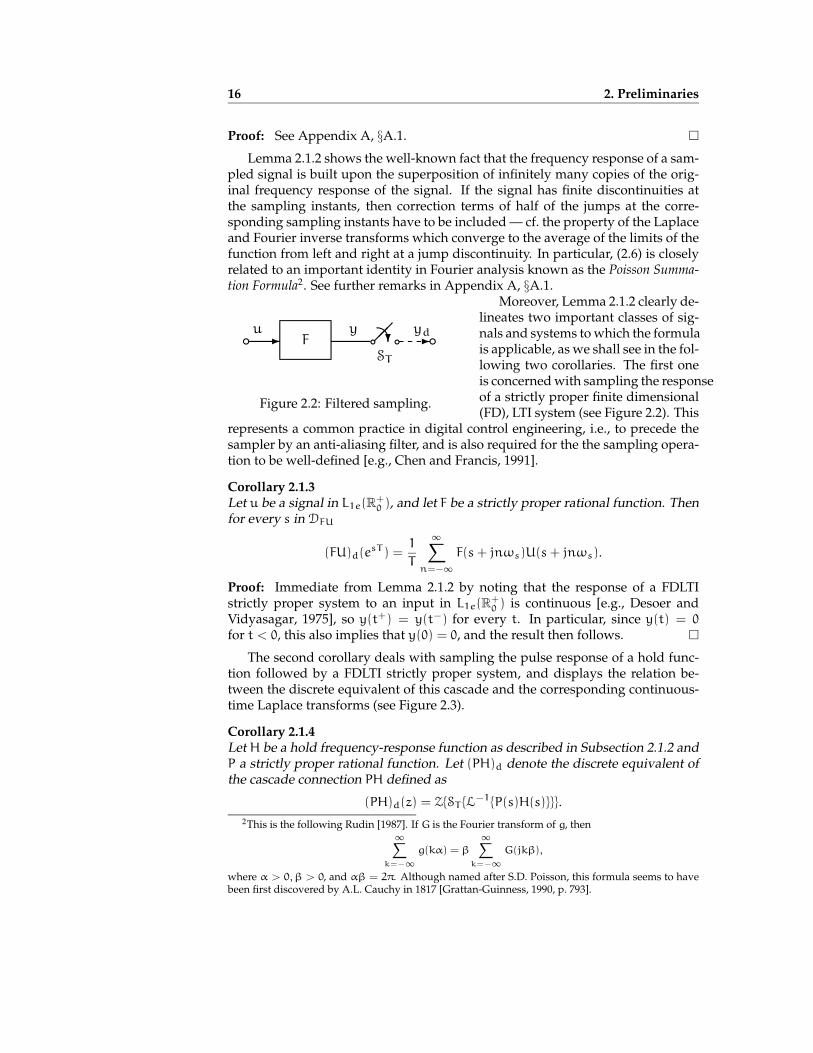
Figure 2.2: Filtered sampling.
lineates two important classes of sig-nals and systems to which the formulais applicable, as we shall see in the fol-lowing two corollaries. The first oneis concerned with sampling the responseof a strictly proper finite dimensional(FD), LTI system (see Figure 2.2). This
represents a common practice in digital control engineering, i.e., to precede thesampler by an anti-aliasing filter, and is also required for the the sampling opera-tion to be well-defined [e.g., Chen and Francis, 1991].
Corollary 2.1.3Let u be a signal in L1e(R+
0 ), and let F be a strictly proper rational function. Thenfor every s in DFU
(FU)d(esT ) =
1
T
∞∑n=−∞ F(s+ jnωs)U(s+ jnωs).
Proof: Immediate from Lemma 2.1.2 by noting that the response of a FDLTIstrictly proper system to an input in L1e(R+
0 ) is continuous [e.g., Desoer andVidyasagar, 1975], so y(t+) = y(t−) for every t. In particular, since y(t) = 0
for t < 0, this also implies that y(0) = 0, and the result then follows.
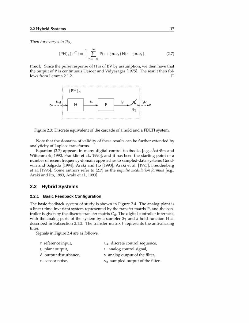
The second corollary deals with sampling the pulse response of a hold func-tion followed by a FDLTI strictly proper system, and displays the relation be-tween the discrete equivalent of this cascade and the corresponding continuous-time Laplace transforms (see Figure 2.3).
Corollary 2.1.4Let H be a hold frequency-response function as described in Subsection 2.1.2 andP a strictly proper rational function. Let (PH)d denote the discrete equivalent ofthe cascade connection PH defined as
(PH)d(z) = ZST L−1P(s)H(s).
2This is the following Rudin [1987]. If G is the Fourier transform of g, then∞∑k=−∞g(kα) = β
∞∑k=−∞G(jkβ),
where α > 0,β > 0, and αβ = 2π. Although named after S.D. Poisson, this formula seems to havebeen first discovered by A.L. Cauchy in 1817 [Grattan-Guinness, 1990, p. 793].
2.2 Hybrid Systems 17
Then for every s in DP,
(PH)d(esT ) =
1
T
∞∑n=−∞P(s+ jnωs)H(s+ jnωs). (2.7)
Proof: Since the pulse response of H is of BV by assumption, we then have thatthe output of P is continuous Desoer and Vidyasagar [1975]. The result then fol-lows from Lemma 2.1.2.
?c bb c-- - -
....................................................................
....................................................................
...
...
...
...
...
...
...
...
...
..
...
...
...
...
...
...
...
...
...
..
u
(PH)d
yP
ST
ydH
ud
Figure 2.3: Discrete equivalent of the cascade of a hold and a FDLTI system.
Note that the domains of validity of these results can be further extended byanalyticity of Laplace transforms.
Equation (2.7) appears in many digital control textbooks [e.g., Astrom andWittenmark, 1990, Franklin et al., 1990], and it has been the starting point of anumber of recent frequency-domain approaches to sampled-data systems Good-win and Salgado [1994], Araki and Ito [1993], Araki et al. [1993], Freudenberget al. [1995]. Some authors refer to (2.7) as the impulse modulation formula [e.g.,Araki and Ito, 1993, Araki et al., 1993].
2.2 Hybrid Systems
2.2.1 Basic Feedback Configuration
The basic feedback system of study is shown in Figure 2.4. The analog plant isa linear time-invariant system represented by the transfer matrix P, and the con-troller is given by the discrete transfer matrix Cd. The digital controller interfaceswith the analog parts of the system by a sampler ST and a hold function H asdescribed in Subsection 2.1.2. The transfer matrix F represents the anti-aliasingfilter.
Signals in Figure 2.4 are as follows,
r reference input,y plant output,d output disturbance,n sensor noise,
uk discrete control sequence,u analog control signal,v analog output of the filter,vk sampled output of the filter.

18 2. Preliminaries
? k
kk bb r
cc
cc -
6
?-
?
- - - - -
T
r
d
n
+ y+
+
+
+
−
uk uv vkF Cd H P
Figure 2.4: Sampled-data control system.
Analog signals are given as functions defined over t in R+0 , while discrete
signals are sequences defined at entire multiples k of the sampling time T . Weshall assume that the input signals satisfy the following condition.
Assumption 2The reference signal r, disturbance d, and noise n are functions in L1e(R+
0 ).
It is straightforward to verify that this assumption is satisfied by signals thatare steps, ramps, sinusoids or exponentials, and signals in Lp(R+
0 ) for 1 ≤ p ≤∞Chen and Francis [1991]. Signals that contain impulses are excluded.
We shall assume throughout that the following conditions are satisfied by theplant, filter, and compensator.
Assumption 3The plant, filter, and compensator are full column rank rational transfer matrices,each free of unstable hidden modes, and they satisfy the following additionalhypotheses,
(i) P(s) = P0(s) e−sτ, where P0 is proper and τ ≥ 0,
(ii) F is strictly proper, stable and minimum-phase, and
(iii) Cd is proper.
The assumption that the filter F is strictly proper is standard and guaran-tees that the sampling operation is well-defined [e.g., Chen and Francis, 1991,Sivashankar and Khargonekar, 1993]. The assumptions that F has no poles orzeros in C+ may be removed, and are only invoked to facilitate discussion. Inpractice anti-aliasing filters will satisfy these assumptions.
We define the discretized plant as the discrete transfer function of the seriesconnection of hold, plant, filter, and sampler,
(FPH)d(z) , ZST L−1F(s)P(s)H(s). (2.8)

2.2 Hybrid Systems 19
It follows from Assumptions 1 and 3, and Corollary 2.1.4 that the discretizedplant satisfies the well-known relation
(FPH)d(esT ) =
1
T
∞∑k=−∞ Fk(s)Pk(s)Hk(s), (2.9)
where the notation Fk(s) represents F(s + jkωs), i.e., the shift of F(·) by an entirenumber of times the sampling frequency in the direction of the imaginary axis.We shall use this notation throughout this thesis.
Suppose now that in the loop of Figure 2.4 we assume r = 0 and consider adisturbance x at the input of the plant. Introduce a ficticious hold at x, and shiftthe filter and sampler to the inputs at the summation point of n, as shown inFigure 2.5. From this diagram we obtain the discrete loop of Figure 2.6.
? bi a a ....................... nnk+
+F
?a a.......................
i i
b b
b- - - - -?
-?
?
?
+
Cd PH− +
H
x
xk
uvk
d
ykF
y
Figure 2.5: Sampled-data system with input disturbances.
We now define the discrete sensitivity and discrete complementary sensitivityfunctions. Since the setup is multiple-input multiple output, there are two pairs offunctions corresponding to the scalar ones, depending where the loop is openedFreudenberg and Looze [1988]. We shall require only the following input discretesensitivity function,
Sd(z) , [I+ Cd(z)(FPH)d(z))]−1, (2.10)
and output discrete complementary sensitivity function,
Td(z) , (FPH)d(z)Sd(z)Cd(z). (2.11)
These functions map signals in the discrete loop of Figure 2.6 as
Ud(z) = Sd(z)Xd(z) and Yd(z) = Td(z)Nd(z),
where Ud, Xd, Yd, andNd correspond to the Z-transforms of the signals ux, xk, yk,and nk, respectively.

20 2. Preliminaries
Cd
?ib bi baa- - -
6
- -
?
........................................................
........................................................
...
...
...
...
...
...
...
...
...
...
...
...
...
...
...
...
- .......................xk
Hykuk
(FPH)d
− nk
P F
Figure 2.6: Discrete sensitivity functions.
2.2.2 Non-pathological Sampling and Internal Stability
As with the case of a ZOH, closed-loop stability is guaranteed by the assumptionsthat sampling is non-pathological and that the discretized system is closed-loopstable. The next result is a generalization of the well-known result of Kalmanet al. [1963] to the case of GSHFs.
Lemma 2.2.1 (Non-pathological Sampling, Middleton and Freudenberg [1995])Suppose that P and F are as defined in Subsection 2.2.1 and assume further that
(i) if λi and λk are CRHP poles of P, then
λi 6= λk + jnωs, n = ±1,±2, · · · (2.12)
(ii) if λi is a CRHP pole of P, then H(s) has no zeros at s = λi.
Then the discretized plant (2.8) is free of unstable hidden modes.
In particular, Lemma 2.2.1 says that since the response of a GSHF may havezeros in C+, it may be necessary to require that none of these coincides with anunstable pole of the analog plant (note that this is necessary in the SISO case). Un-der the non-pathological sampling hypothesis, it is straightforward to extend theexponential and L2 input-output stability results of Francis and Georgiou [1988]and Chen and Francis [1991] to the case of GSHF.
Lemma 2.2.2Suppose that P, F, Cd, and H are as defined in Subsections 2.1.2 and 2.2.1, thatthe nonpathological sampling conditions (i) - (ii) are satisfied, that the product(FPH)d Cd has no pole-zero cancelations in DC, and that all poles of Sd lie inD. Then the feedback system in Figure 2.4 is exponentially stable and L2 input-output stable.
Proof: The proof may be obtained by simple modification of the proofs of Fran-cis and Georgiou [1988, Theorem 4] and Chen and Francis [1991, Theorem 6].
Lemma 2.2.2 establishes the conditions for the nominal stability of the sampled-data system of Figure 2.4, and will be required in most of the remaining chapters.In particular, this result guarantees that the operators mapping disturbances andnoise to the output are bounded on L2. This will be the starting point for theanalysis developed in Chapter 5.

2.3 Summary 21
2.3 Summary
This chapter has introduced the main notation, definitions, and preliminary re-sults that will be required in the rest of this thesis.


3Generalized Sampled-data
Hold Functions
Generalized Sampled-data Hold Functions [e.g., Kabamba, 1987, Bai and Das-gupta, 1990, Yan et al., 1994, Er et al., 1994] have been proposed as an approachto several control problems that do not have answers with analog LTI, or tra-ditional sampled-data settings based on the ZOH. GSHF-based control schemesare sampled-data systems where the D-A conversion is performed using a specialwaveform instead of the constant function generated by the ZOH (see Figure 3.1).The choice of this waveform is an additional degree of freedom incorporatedto the design, and it seems to give a number of advantages over other controlschemes. For example, it has been recently shown that if there exist a solution tothe H∞ control problem for sampled-data systems, then this solution can be im-plemented by a GSHF following a LTI discrete controller. [e.g., Sun et al., 1993].
However, serious robustness and sensitivity problems associated with the useof GSHFs have been pointed out by some authors Feuer and Goodwin [1994],Zhang and Zhang [1994] showing that many of the most impressive features ofGSHFs come along with quite undesirable “side-effects”. For example, Feuer andGoodwin [1994] have shown that the arbitrary shaping of the sampled frequencyresponse of a system by means of a GSHF necessarily relies on the generationof high frequency components in the continuous-time output. This exposes themechanism by which sensitivity and robustness properties of the system are com-promised, since in practice high frequency uncertainty is very common.
Furthermore, as we shall see in Chapter 4, there are essential continuous-timedesign limitations that are inherited by the sampled-data system, irrespective ofthe particular discretization method employed. Particularly linked to these is-sues are the frequency response and the zeros of the hold device. It turns out, forexample, that “non-minimum phase” holds, i.e., holds with zeros in C+, imposeextra limitations in the achievable continuous-time performance of the system.These “non-minimum phase” zeros of the hold may also lead to poorly condi-tioned discretized systems, as has been discussed by Middleton and Freudenberg[1995] and Middleton and Xie [1995].
In this chapter, we study the frequency response and zero distribution ofGSHFs. The results obtained here allow us to go deeper into the understanding

24 3. Generalized Sampled-data Hold Functions
T
GSHF
ZOH
Figure 3.1: D-A conversion with ZOH and GSHF
of the design tradeoffs associated with the use of these devices. For example, oneof the key results of this chapter is that holds with “asymmetric” pulse responsewill necessarily have zeros off the jω-axis, which may lead to the aforementioneddifficulties.
The organization of the chapter is as follows. In §3.1, we collect several prop-erties of the frequency response of a GSHF. Among these properties are someinteresting relations between the frequency response of a generalized hold andthat of a ZOH. The distribution of zeros of GSHFs is the theme of §3.2. In §3.3, weestablish some connections between these zeros and the values of the frequencyresponse on the jω-axis. Finally, we provide some concluding remarks in §3.4.
3.1 Frequency Response of Generalized Sampled-data Holds
The most standard and simplest D-A converter in digital control implementationsis the ZOH. Given a discrete input sequence uk
∞k=0, the ZOH is defined by
u(t) = uk, for kT ≤ t < (k+ 1)T.
In particular, the ZOH can be seen as a particular case of the GSHF defined in(2.3) with the hold function
h(t) =
1 t ∈ [0, T)
0 otherwise
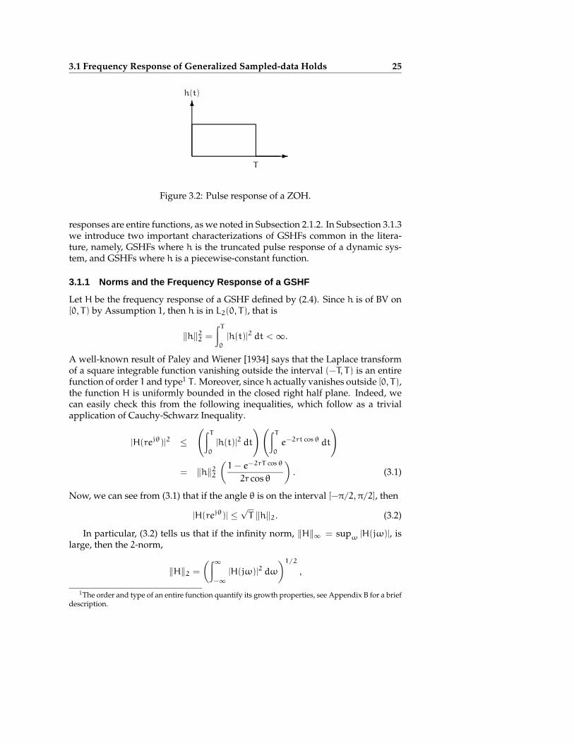
(see Figure 3.2).The idea of a GSHF is to allow h to be some suitably chosen function instead
of just holding the discrete values constant during the sampling interval. In thisway a new degree of freedom is introduced in the sampled-data control designproblem, in addition to the choice of the discrete controller.
In this section we present some preliminary results concerning the frequencyresponse of a GSHF. In Subsections 3.1.1 and 3.1.2, we obtain some general prop-erties of the frequency response of a GSHF, norms and reconstruction from bound-ary values. These properties are intimately linked to the fact that GSHF frequency
3.1 Frequency Response of Generalized Sampled-data Holds 25
6
-
h(t)
T
Figure 3.2: Pulse response of a ZOH.
responses are entire functions, as we noted in Subsection 2.1.2. In Subsection 3.1.3we introduce two important characterizations of GSHFs common in the litera-ture, namely, GSHFs where h is the truncated pulse response of a dynamic sys-tem, and GSHFs where h is a piecewise-constant function.
3.1.1 Norms and the Frequency Response of a GSHF
Let H be the frequency response of a GSHF defined by (2.4). Since h is of BV on[0, T) by Assumption 1, then h is in L2(0, T), that is
‖h‖22 =
∫T0
|h(t)|2 dt <∞.A well-known result of Paley and Wiener [1934] says that the Laplace transformof a square integrable function vanishing outside the interval (−T, T) is an entirefunction of order 1 and type1 T . Moreover, since h actually vanishes outside [0, T),the function H is uniformly bounded in the closed right half plane. Indeed, wecan easily check this from the following inequalities, which follow as a trivialapplication of Cauchy-Schwarz Inequality.
|H(rejθ)|2 ≤
(∫T0
|h(t)|2 dt
)(∫T0
e−2rt cosθ dt
)
= ‖h‖22(1− e−2rT cosθ
2r cos θ
). (3.1)
Now, we can see from (3.1) that if the angle θ is on the interval [−π/2, π/2], then
|H(rejθ)| ≤√T ‖h‖2. (3.2)
In particular, (3.2) tells us that if the infinity norm, ‖H‖∞ = supω |H(jω)|, islarge, then the 2-norm,
‖H‖2 =
(∫∞−∞ |H(jω)|2 dω
)1/2,
1The order and type of an entire function quantify its growth properties, see Appendix B for a briefdescription.

26 3. Generalized Sampled-data Hold Functions
will also be large, since by Parseval’s Formula ‖H‖2 =√2π ‖h‖2.
Another interesting connection between frequency and time domain values isgiven by the following lemma [cf. Yamamoto and Araki, 1994, Lemma 3.3].
Lemma 3.1.1 (Parseval’s Equality for Holds)For any real numberω and any H defined by (2.4),
1
T
∞∑k=−∞ |H(jω+ jkωs)|
2 = ‖h‖22 (3.3)
Proof: Consider the function fω(t) = h(t) e−jωt, with support on the interval[0, T). Its Fourier series representation is
fω(t) =
∞∑k=−∞ ck e
jkωst, for t in [0, T)
where the Fourier coefficients are
ck =1
T
∫T0
fω(t) e−jkωst dt
=1
TH(jω+ jkωs) (3.4)
Hence, by Parseval’s Formula we have that
1
T
∫T0
|fω(t)|2 dt =
∞∑k=−∞ |ck|
2.
The result is then obtained by noting that |fω(t)| = |h(t)|, and replacing ck from(3.4).
An interpretation in terms of frequency aliasing can be given to the above result.Suppose that H(0) 6= 0, i.e., the hold has non-zero DC-gain, and (without loss ofgenerality) assume thatH(0) = 1. If |H(jω)| has a large peak, say ‖H‖∞ 1, thenfrom (3.2) and (3.3) follows that
∞∑k=−∞ |H(jω+ jkωs)|
2 1. (3.5)
Hence, evaluation of (3.5) at small values ofω still gives a large sum, and so theremust be a significant number of other terms (k 6= 0) adding to |H(jω)| to give alarge 2-norm. Thus, a peak of |H(jω)| necessarily implies a lot of frequency “fold-ing” going on. In particular, note that since HZOH has zeros at integer multiplesof the sampling frequency ωs, then the ZOH has the minimum L2-norm over allthe holds that satisfy H(0) = 1.
Yet a last property of GSHFs gives us the “gain” of the hold viewed as aninput-output operator. Let H denote the hold operator mapping `p to Lp, 1 ≤p ≤ ∞, defined by (2.3). The lemma below is a generalization to GSHFs of aresult for the ZOH in Francis [1991].

3.1 Frequency Response of Generalized Sampled-data Holds 27
Lemma 3.1.2 (Input-output norm of a hold operator)The hold operator H : `p → Lp is bounded and of norm ‖h‖p.
Proof: We prove this for p <∞; the case p =∞ follows similar steps. Let u be afunction in Lp, and v = vk
∞k=−∞ a sequence in `p, such that u = Hv. Then,
‖u‖pp =
∫∞−∞ |u(t)|p dt
=
∞∑k=−∞
∫ (k+1)T
kT
|h(t− kT)vk|p dt
=
(∫T0
|h(t)|p dt
)( ∞∑k=−∞ |vk|
p
)= ‖h‖pp ‖v‖pp.
In particular, Lemma 3.1.2 tells us that the induced norm of the hold operator inthe case of bounded-input, bounded-output (BIBO) spaces (p = ∞) is precisely‖h‖∞. Therefore, we see that a large value of ‖h‖∞ implies a “high gain” hold,viewed as a BIBO device. Combining (3.2) with the fact that ‖h‖2 ≤
√T ‖h‖∞,
we obtain‖H‖∞ ≤ T ‖h‖∞.
So, we see that, for a given sampling rate, a large peak in |H(jω)| also implies alarge BIBO gain. Since the output of the hold is typically the input to the plant,such large gain may introduce serious difficulties due to actuator saturations,present in most real systems Gilbert [1992].
3.1.2 GSHF Frequency Responses from Boundary Values
Analytic functions can be reconstructed from their boundary values by means ofintegral formulas like Poisson’s or Cauchy’s [e.g., Hoffman, 1962]. Not surpris-ingly, since they are entire functions, GSHF frequency responses can be recov-ered from similar relations. The interesting fact is that the frequency response ofa ZOH is involved in these reconstructions. In this subsection we present tworesults on reconstruction from boundary values of the frequency response of aGSHF.
Denote by HZOH the response of a ZOH,
HZOH(s) =1− e−sT
s.
The following lemma is a straightforward consequence of the Fourier representa-tion of h [See also Feuer and Goodwin, 1996].

28 3. Generalized Sampled-data Hold Functions
Lemma 3.1.3 (Hold Response from Boundary Values: “Discrete” Version)For any complex number s and any H defined by (2.4),
H(s) =1
T
∞∑k=−∞H(jkωs)HZOH(s− jkωs) (3.6)
Proof: Expand h into Fourier series,
h(t) =
∞∑K=−∞ ck e
jkωst, where ck =1
T
∫T0
h(t) e−jkωst dt = H(jkωs). (3.7)
Then, the Laplace transform of (3.7) gives
H(s) =1
T
∞∑k=−∞H(jkωs)
1− e−sT
s− jkωs,
completing the proof.
Interestingly, there exists a — not so obvious — “continuous” version of theabove formula, arising from properties of Paley-Wiener spaces of entire functionsDe Branges [1968].
Lemma 3.1.4 (Hold Response from Boundary Values: “Continuous” Version)For any complex number s and any H defined by (2.4),
H(s) =1
2π
∫∞−∞H(jω)HZOH(s− jω)dω (3.8)
Proof: If f is a function that vanishes outside the interval [−T/2, T/2], and itsLaplace transform, F, is such that
∫∞−∞ |F(jω)|2dω < ∞, then F is an entire func-
tion of type T/2 [De Branges, 1968, p. 45]. Moreover, for any complex numbers,
F(s) =
∫∞−∞ F(jω)
sinh(jωT/2− sT/2)
π(jω− s)dω. (3.9)
Applying (3.9) to the function H(s) e−sT/2 gives the result.
3.1.3 Two Simple Classes of GSHFs
To further study properties of the frequency responses of GSHFs we need to de-scribe them in greater detail. In this subsection we present two different classesof GSHFs that are important for their simple mathematical description. Theseholds have been suggested by different authors, and were studied in the presentformulation by Middleton and Freudenberg [1995].
The first class of GSHFs is characterized by a pulse response h generated asthe response of a finite dimensional linear time-invariant system truncated tohave support on the interval [0, T) (see Figure 3.3). This family covers, for ex-ample, the type of GSHFs suggested by Kabamba [1987] to achieve simultaneous

3.1 Frequency Response of Generalized Sampled-data Holds 29
h(t)
T
Figure 3.3: Pulse response of aFDLTI GSHF.
6
-
h(t)
T
Figure 3.4: Pulse response of a PCGSHF.
stabilization of a finite number of continuous-time plants, decoupling, discretemodel matching, discrete simultaneous optimal noise rejection, and arbitrarygain-margin improvement [See also Bai and Dasgupta, 1990, Liu et al., 1992, Had-dad et al., 1994, Yang and Kabamba, 1994, Paraskevopoulos and Arvanitis, 1994].
Definition 3.1.1 (Finite Dimensional Linear Time-invariant GSHF)Given suitably dimensioned matrices K, L and M, we define a finite dimensionallinear time-invariant GSHF (FDLTI GSHF) by the pulse response
h(t) = KeL(T−t)M, for t ∈ [0, T). (3.10)
FDLTI GSHFs have a simple and convenient model for analysis and design ofGSHF-based control systems. Yet, this model still seems an impractical schemefor implementation.
The second class of GSHFs is characterized by a piecewise-constant pulse re-sponse function h, typically with a regular partition ofN subintervals of the sam-pling interval [0, T) (see Figure 3.4). Clearly [e.g. Yan et al., 1994], this type ofholds can arbitrarily approximate any GSHF of the form (3.10) by taking N suf-ficiently large and, in addition, appears as a much more feasible alternative fora practical implementation. Holds of this class have been suggested for discreteloop transfer recovery, and arbitrary gain-margin improvement of continuous-time non-minimum phase linear systems [Yan et al., 1994, Er et al., 1994, Er andAnderson, 1994].
Definition 3.1.2 (Piecewise-constant GSHF)A piecewise-constant GSHF (PC GSHF) is given by the following pulse response:
h(t) =
a0 if t ∈ [0, T/N),
a1 if t ∈ [T/N, 2T/N),
. . . . . .
aN−1 if t ∈ [(N− 1)T/N, T).
(3.11)

30 3. Generalized Sampled-data Hold Functions
The frequency response functions for FDLTI and PC GSHFs can be easily com-puted from their definitions, and are given by the following lemmas taken fromMiddleton and Freudenberg [1995].
Lemma 3.1.5 (Frequency Response Function of a FDLTI GSHF)The frequency response function of a FDLTI GSHF defined by (3.10) is:
H(s) = K(sI+ L)−1(eLT − e−sT I)M. (3.12)
Lemma 3.1.6 (Frequency Response Function of a PC GSHF)The frequency response function of a PC GSHF defined by (3.11) is:
H(s) =1− e−sT/N
sAd(e
−sT/N), (3.13)
where Ad(z) is the polynomial
Ad(z) ,N−1∑k=0
ak zk. (3.14)
In the rest of the chapter we shall assume that the following additional condi-tion is satisfied by the pulse response h.
Assumption 4The hold function h is non-zero almost everywhere in neighborhoods of t = 0
and t = T .
This is a technical condition required only for simplicity of analysis; it may beremoved at the expense of more complexity in the notation. This assumption maybe interpreted as that the hold pulse response h has “effective” support on thewhole interval [0, T), e.g., no pure time-delays. This is clearly satisfied by FDLTIGSHFs, as is easily seen from (3.12). For PC GSHFs Assumption 4 is equivalentto a0 6= 0 6= aN−1.
3.2 Distribution of Zeros of GSHFs
Zeros of a hold response function have important connections with fundamentalproperties of the sampled-data system. For example, Middleton and Freudenberg[1995] have shown that these zeros have transmission blocking properties andcan also affect the stabilizability properties of the discretized system (cf. §2.2.2 inChapter 2). Furthermore, zeros of the hold in C+ impose design tradeoffs in theachievable performance of the sampled-data system, as we shall see in Chapter 4.
This section focuses on the distribution of zeros of the hold frequency re-sponse H. In Subsection 3.2.1 we describe the precise location and asymptotic

3.2 Distribution of Zeros of GSHFs 31
distribution of the zeros of PC and FDLTI holds. Apart from the mentioned ef-fects of “non-minimum phase” zeros on the system performance, it turns out —and we shall see it in §3.3 — that all zeros compromise the shape of the holdfrequency response on the jω-axis. In Subsection 3.2.2, we derive a necessarycondition for these GSHFs to have frequency responses with all their zeros onthe jω-axis. We finish in Subsection 3.2.3 with an example that illustrates theseresults.
3.2.1 Zeros of PC and FDLTI GSHFs
It is difficult to make general statements about the distribution of the zeros of aGSHF. However, for important special cases, the locations and asymptotic distri-bution of these zeros can be described precisely. The following lemma character-izes exhaustively the zeros of PC holds, which are the GSHFs of greatest practicalsignificance.
Lemma 3.2.1 (Zeros of a Piecewise-constant GSHF)Consider a GSHF given by (3.11) with associated frequency response function Hgiven by (3.13) and (3.14). Then the zeros of H are at
s = j`Nωs, where ` = ±1,±2, . . . , (3.15)
ands = −
N
Tlog ξi + jkNωs, with k = 0,±1,±2, . . . , (3.16)
where ξi, with i = 1, 2, . . . ,N, is any zero of Ad(z).
Proof: From Lemma 3.1.6, H can be written as (3.13). The zeros of
1− e−sT/N
s
are given by (3.15). It remains, therefore, to determine the zeros of Ad(e−sT/N),which are given precisely by (3.16). The assumption that a0 6= 0 implies thatξi 6= 0 for every i, and hence log ξi is defined.
This result tells us that the zeros of a PC GSHF are essentially determined bythose of the polynomial Ad, and the sampling period.
Zeros of FDLTI holds are harder to determine, but we can say something inparticular cases. Consider a hold defined by (3.10), and suppose that h is notidentically zero. Letm and n be the smallest nonnegative integers such that
h(m)(0+) 6= 0 and h(n)(T−) 6= 0, (3.17)
where h(k) denotes the kth-derivative of h. We define
η ,h(m)(0+)
h(n)(T−), (3.18)

32 3. Generalized Sampled-data Hold Functions
which, for the particular case of FDLTI GSHFs, equals
η =K(−L)meLTM
K(−L)nM.
Then we have the following result concerning the asymptotic locations of thezeros of FDLTI GSHFs.
Lemma 3.2.2 (High Frequency Zeros of a FDLTI GSHF)If H is the frequency response of a FDLTI GSHF, then it has an unbounded se-quence of zeros γ`
∞=1 “converging to infinity”. Furthermore, these zeros con-
verge to the roots of the equation η = e−φTφn−m. In particular, if n = m, thezeros converge to the sequence defined by
φ` = −1
Tlogη+ j`ωs, ` = 0,±1,±2, . . . (3.19)
Proof: See §A.2 in Appendix A.
A precise description of the zeros of a FDLTI hold is possible in a particularcase, as we see in the following lemma.
Lemma 3.2.3 (Zeros of a FDLTI GSHF (Special Case))Consider a FDLTI GSHF, and suppose that KM 6= 0. Assume that L = λI, whereI is the identity matrix and λ is a scalar. Then the zeros of H are located preciselyat
γ` = −λ+ j`ωs, ` = ±1,±2, . . . (3.20)
Proof: Since KM 6= 0,H is not identically zero. The special structure of L impliesthat
H(s) = KMeλT − e−sT
s+ λ,
and the result follows.
Remark 3.2.1 (Approximation of the zeros of a FDLTI GSHF) Notice that sincea FDLTI GSHF will most probably be implemented as a PC GSHF, the additionaldifficulty in characterizing zeros of FDLTI holds over PC holds is somehow de-prived of practical significance2.
3.2.2 GSHFs with all Zeros on the jω-axis
A well-known property of a hybrid control system using a ZOH in conjunctionwith a discrete integrator is the ability to asymptotically reject step disturbances.This arises from the fact that the ZOH frequency response has zeros at multiplesof the sampling frequencyωs = 2π/T on the jω-axis,
HZOH(jkωs) = 0, for k = ±1,±2, . . . .2See the example in Subsection 3.2.3.

3.2 Distribution of Zeros of GSHFs 33
In addition, these zeros contribute to diminish high frequency components ofthe plant response that are aliased down to low frequencies. This is particularlyimportant in sampled-data control applications, where the low-frequency rangeis typically of great interest.
The response of a GSHF, on the other hand, need not have zeros at these fre-quencies, and thus high frequency plant behavior (and uncertainty) may havesignificant effect on the low-frequency range of the hybrid control system [cf.Feuer and Goodwin, 1994]. To get a preliminary intuitive view of this, comparefor example the GSHF response with the response of a ZOH, plotted in Figure 3.5;this GSHF is taken from Kabamba [1987, Example 2].
GSHFZOH
10−2
10−1
100
101
102
10−4
10−3
10−2
10−1
100
101
102
Frequency [rad/s]
|H(jw
)|
Figure 3.5: Frequency response of hold functions.
In addition, zeros ofH close to unstable open-loop poles of the plant may ren-der an ill-conditioned discrete-time system Middleton and Freudenberg [1995],Middleton and Xie [1995], due to an approximate pole-zero cancelation that tendto violate the non-pathological sampling assumption of Lemma 2.2.1. Moreover,as will become clear in §3.3, also zeros in C− compromise the frequency responseof the hold, depending on the specifications that this frequency response is re-quired to meet.
An interesting question then arises from the above observations: What is theclass of GSHFs that, as the ZOH, have all their zeros on the jω-axis? The fol-lowing proposition gives a necessary condition that the hold frequency responsemust satisfy to have such a zero distribution.
Proposition 3.2.4Let H be the frequency response function of a PC or a FDLTI GSHF; suppose thath satisfy Assumption 4. Then if H has all its zeros on the jω-axis, either
H(s) = e−sT H(−s), (3.21)
orH(s) = −e−sT H(−s). (3.22)

34 3. Generalized Sampled-data Hold Functions
Proof: Suppose that jak are the nonzero zeros of H repeated according to mul-tiplicity, and thatH has a zero at z = 0 of order p ≥ 0 (p = 0means thatH(0) 6= 0).Since H is an entire function of exponential type T , using the Hadamard Factor-ization Theorem [e.g., Markushevich, 1965] we can represent it as
H(s) = speg0+g1s∞∏k=1
(1−
s
jak
)es/jak , (3.23)
where g0 and g1 are real numbers. Without lost of generality we may assumeg0 = 0 (since otherwise we considerH(s)e−g0), and since the zeros are symmetricwith respect to the real axis, (3.23) simplifies to
H(s) = speg1s∞∏`=1
(1+
s2
a2`
), (3.24)
where now a` denote the zeros in the upper (or lower) half of the jω-axis.As in Subsection 3.2.1 let m and n be the smallest integers such that (3.17)
holds. Notice that both h(m)(0+) and h(n)(T+) are nonzero finite numbers for PCand FDLTI GSHFs with compact support on [0, T). Hence, the number η definedin (3.18) is also nonzero and finite. Next we use the Initial Value Theorem [e.g.,Zemanian, 1965] to compute h(n)(0+) from (3.24). Thus, for x real we have that
h(m)(0+) = limx→∞ xm+1H(x)
= limx→∞ xp+m+1eg1x
∞∏k=1
(1+
x2
a2`
). (3.25)
An analogous expression can be obtained for h(n)(T−) following similar stepswith H(−s)e−sT ,
h(n)(T−) = limx→∞(−x)n+1e−xTH(−x)
= limx→∞(−1)n+pxp+n+1e−(g1+T)x
∞∏k=1
(1+
x2
a2`
). (3.26)
Therefore, we can write from (3.25) and (3.26),
η =h(m)(0+)
h(n)(T−)
= limx→∞(−1)n+pxm−ne(2g1+T)x. (3.27)
Since η is nonzero and finite, it necessarily follows from (3.27) that m = n andg1 = −T/2. With this value of g1 in (3.24), it is easy to check that H verifies therequired conditions (3.21) or (3.22) (the sign depending on the order of the zeroat s = 0), completing the proof.

3.2 Distribution of Zeros of GSHFs 35
Notice in the proof above that the conditions m = n, and g1 = −T/2 implythat η = (−1)n+p, which in turn, by Lemma 3.2.2, tells us that the zeros of Happroach asymptotically to the jω-axis as the distance from the origin increases.We could say then that conditions (3.21) and (3.22) become also “sufficient” forlarge values of s.
The fact that η = (−1)n+p also suggests that if H has all its zeros on the jω-axis, then h has some kind of symmetry with respect to the middle point of theinterval [0, T). For example, if n = 1 and p = 0 say, then h(0+) = 0 = h(T−),and the corresponding derivatives are mirrored, h ′(0+) = −h ′(T−). In fact, con-ditions (3.21) and (3.22) are equivalent to “symmetry” of h, as we shall prove next.Let us first make more precise what we mean by this.
Definition 3.2.1 (Symmetry of h)We say that h has even (odd) symmetry if h(t) = h(T − t) (h(t) = −h(T − t)). Wesay that h is symmetric if h has either even or odd symmetry.
The following corollary to Proposition 3.2.4 establishes that holds with alltheir zeros on the jω-axis are necessarily symmetric in the sense just defined.
Corollary 3.2.5If H has all its zeros on the jω-axis, then h is symmetric. Moreover,
(i) ifH has none or an even number of zeros at s = 0, then h is even symmetric;
(ii) if H has an odd number of zeros at s = 0, then h is odd symmetric.
Proof: We prove only (i); the proof of (ii) is obtained in a similar way. We knowfrom Proposition 3.2.4 that if H has all its zeros on the jω-axis — and none or aneven number of them at s = 0, then condition (3.21) is satisfied. Write the FourierSeries representation of h,
h(t) =
∞∑k=−∞ ck e
jkωst, (3.28)
with
ck =1
T
∫T0
e−jkωst h(t)dt
=H(jkωs)
T.
We prove now that condition (3.21) is satisfied if and only if all ck — i.e.,H(jkωs)— are real. Indeed, if ck is real for all k, then H(jkωs) = H(−jkωs), and using

36 3. Generalized Sampled-data Hold Functions
Lemma 3.1.3 we have that
H(s) =1
T
∞∑k=−∞H(jkωs)HZOH(s− jkωs)
=1
T
∞∑`=−∞H(j`ωs)HZOH(s+ j`ωs)
=e−sT
T
∞∑`=−∞H(j`ωs)HZOH(−s− j`ωs)
= e−sTH(−s).
The converse is immediate. Finally, (i) follows easily from noting that h has allreal Fourier coefficients if and only if it is even symmetric.
This corollary provides an easy way of determining whether the hold fre-quency responseHmay have zeros off the jω-axis by just examining the shape ofthe hold function h; i.e., an asymmetric hwill necessary imply zeros in either C+
or C−.
Remark 3.2.2 (A Conjecture for a General GSHF) Strictly, we have proved theseresults only for PC and FDLTI GSHFs; nevertheless, we could conjecture that theyhold for the general case. Indeed, notice that any admissible h can be arbitrarilyapproximated by a piecewise-constant function hPC, and then the zeros of HPCwill approximate the zeros of H. Then, it is clear that if H has all its zeros onthe jω-axis, we can build a sequence of symmetric PC functions whose zeros willapproach to the jω-axis. Since the result holds for HPC, we can expect that, in thelimit, it will hold also for H. A rigorous proof seems difficult, though.
3.2.3 Example: Zeros of a FDLTI GSHF
In this example we illustrate the previous results on zero locations of GSHFs. Weconsider the FDLTI GSHF used in Kabamba [1987, Example 2] to simultaneouslystabilize two continuous-time systems that violate the appropriate parity inter-lacing property (cf. Example 7.1.1). The matrices that define the hold functionwith the characterization given by Definition 3.1.1 are
K =[1 0 0
], L =
1 1 0
2 0 1
0 0 0
, M =
87.5619
−616.49371322.6
.The sampling period is T = 1s, to which corresponds a sampling frequency
ωs = 2π. The hold function h is shown on the left in Figure 3.6.As we can see in the figure, h is not symmetric, so we know by Corollary 3.2.5
that the corresponding frequency response H will have zeros off the jω-axis. In-deed, this can be seen in Figure 3.7, where we have plotted a section of the func-tion log |H| for s = x + jy, with −1.5 ≤ x ≤ 0.5 and −ωs/2 ≤ y ≤ 3ωs. The zeros

3.2 Distribution of Zeros of GSHFs 37
0 0.5 1−140
−120
−100
−80
−60
−40
−20
0
20
40
60
t
h(t)
jy/ω
s
−1.5 −1 −0.5 0 0.5−0.5
0
0.5
1
1.5
2
2.5
3
x
Figure 3.6: Hold function h, and contour plot of H.
x jy/ω s
−2−1
01 0
12
3−4
−3
−2
−1
0
1
2
3
4
5
log(
|H(s
)|)
Figure 3.7: Zeros of H.

38 3. Generalized Sampled-data Hold Functions
are indicated by the negative peaks on this surface; a contour plot is given on theright in Figure 3.6.
Let us check the asymptotic behavior of the zeros ofH. Following the notationof Lemma 3.2.2 we compute η from (3.18), which, for the values of K, L, and Mgiven is η = 1.4718, with n = 0 = m. Then, by Lemma 3.2.2 we know that thereis an infinite sequence of zeros that approach asymptotically to a sequence givenby (3.19), which for this case is
φ` = −0.3865+ j`ωs. (3.29)
This is can be anticipated already in Figure 3.6, where for reference we havedrawn a vertical line at x = −0.3865.
As we discussed in Remark 3.2.1, the zeros of a FDLTI GSHF can be ap-proximated by the zeros of a PC GSHF, which are completely characterized inLemma 3.2.1. This is verified in Figures 3.8, 3.9, and 3.10, where we have de-picted analogs to Figure 3.6 for PC approximations to hwith 4, 32, and 256 parti-tions respectively. We can see there how the zeros approach to the locations givenin Figure 3.6 as the number of partitions is increased. Notice, however, that theconvergence is slow, particularly for those zeros on the real axis.
0 0.5 1−140
−120
−100
−80
−60
−40
−20
0
20
40
60
t
h(t)
jy/ω
s
−1.5 −1 −0.5 0 0.5−0.5
0
0.5
1
1.5
2
2.5
3
x
Figure 3.8: PC approximation to h, N = 4.
3.3 Integral Relations
Integral relations quantifying inherent limitations in the achievable performanceof feedback control systems have been known for some time. Bode and Poisson

3.3 Integral Relations 39
0 0.5 1−140
−120
−100
−80
−60
−40
−20
0
20
40
60
t
h(t)
jy/ω
s
−1.5 −1 −0.5 0 0.5−0.5
0
0.5
1
1.5
2
2.5
3
x
Figure 3.9: PC approximation to h, N = 32.
0 0.5 1−140
−120
−100
−80
−60
−40
−20
0
20
40
60
t
h(t)
jy/ω
s
−1.5 −1 −0.5 0 0.5−0.5
0
0.5
1
1.5
2
2.5
3
x
Figure 3.10: PC approximation to h, N = 256.

40 3. Generalized Sampled-data Hold Functions
integrals on the sensitivity and complementary sensitivity functions of continuous-time systems have been used to describe design tradeoffs arising from the feed-back structure, and the requirement of closed-loop stability Freudenberg andLooze [1985]. Similar results have been also extended to discrete-time systemsSung and Hara [1988], Middleton and Goodwin [1990]. In Chapter 4 we shallstudy the case of sampled-data systems.
In this section, we present two types of integral relations for the frequencyresponse of a GSHF. These integrals translate the connection between growthcharacteristics and the distribution of zeros into constraints that the magnitudeof the frequency response of the GSHF must satisfy on the jω-axis. We show howzeros off the jω-axis impose tradeoffs over the values of the frequency responseof the hold at all frequencies. In contrast, a zero on the jω-axis only imposes aconstraint at one point (namely, the frequency response is zero at that frequency).
3.3.1 Poisson Integral for GSHFs
Let H be the frequency response function of a GSHF defined by (2.4). Recall thedefinition of the Poisson kernel for the half plane, [e.g., Freudenberg and Looze,1988]. Let s = x + jy, s in C, and let ω be a real number. We define the Poissonkernel for the half plane, Ψ(s,ω), by
Ψ(s,ω) ,x
x2 + (ω− y)2+
x
x2 + (ω+ y)2. (3.30)
The following proposition presents a Poisson integral relation for the function1−H.
Proposition 3.3.1 (Poisson integral for 1−H)Let ξ = x+ jy be a zero of H. Then
(i) if x > 0, ∫∞0
log |1−H(jω)|Ψ(ξ,ω)dω ≥ 0; (3.31)
(ii) if x < 0, ∫∞0
log |1−H(jω) ejωT |Ψ(−ξ,ω)dω ≥ 0. (3.32)
Proof: We prove only (3.31); (3.32) is obtained in a similar way. Consider thefunction F = 1−H. Since H is entire, so is F, and therefore, we may factorize it as
F = F B,
where F is an entire function without zeros in C+, and B is the Blaschke productof the sequence of zeros of F, φk
Nφk=1 (with Nφ possibly infinite), in C+,
B =
Nφ∏k=1
φk − s
φk + s.

3.3 Integral Relations 41
Note that log F is analytic in C+, and furthermore, it satisfies the conditions fora Poisson Integral representation Freudenberg and Looze [1988]. Hence, we canwrite, ∫∞
0
log |F(jω)|Ψ(s,ω)dω = π log |F(s)|
= π log |F(s)| − π log |B(s)|. (3.33)
Evaluating (3.33) at a zero of H in C+, and noting that |F(jω)| = |F(jω)| and− log |B(s)| ≥ 0 for each s in C+, we get inequality (3.31), completing the proof.Inequality (3.32) is obtained similarly by starting with the function F(s) = 1 −H(−s) e−sT .
It follows from (3.31) and (3.32) that zeros of the hold off the jω-axis imposedesign tradeoffs on its frequency response. More specifically, if we require that|H(jω)| be close to 1 over some range of frequencies, |H(jω)| will necessarily showa peak somewhere else. The extent of this difficulty is linked to the relative lo-cation of these zeros, and depends on the specifications that the hold frequencyresponse is required to satisfy on the low-frequency range, as we see next.
Consider an interval of low frequencies Ω = [0,ωb], where ωb ≤ ωs/2, andsuppose that we require the hold response H(jω) to be close to 1 over this inter-val. The interval Ω may be interpreted as the closed-loop bandwidth of a hybridfeedback system with hold H. Asking H(jω) not too large on Ω is a reasonablespecification in practice, since a “high gain” hold may bring in difficulties withactuator saturations (cf. Lemma 3.1.2 and the discussion following). We state thisrequirement as
|1−H(jω)| < α, forω inΩ = [0,ωb], (3.34)
where α is a small positive number.Assume that H has a zero ξ = x + jy in either C+ or C−. Let Θ(ξ,Ω) denote
the weighted length of the intervalΩwith the Poisson kernel for the half plane,
Θ(ξ,Ω) ,∫ωb0
Ψ(ξ,ω)dω, (3.35)
It is not difficult to check that
Θ(ξ,Ω) = arctan(ωb − y
x
)+ arctan
(ωb + y
x
).
As discussed in Freudenberg and Looze [1985] and Freudenberg and Looze [1988],the weighted length Θ(ξ,Ω) may also be interpreted as a phase lag introducedby the term of a Blaschke product corresponding to the zero ξ over Ω; e.g., if ξ isreal, then
Θ(ξ,Ω) = −^ξ− jωs
ξ+ jωs; (3.36)

42 3. Generalized Sampled-data Hold Functions
i.e., the weighted length of the interval Ω equals the negative of the phase lagcontributed by the Blaschke product (ξ− s)/(ξ+ s) at the upper end point of theinterval.
The following result is a straightforward consequence of Proposition 3.3.1.
Corollary 3.3.2Suppose that |H(jω)| satisfies (3.34). Then, if ξ = x+ jy is a zero of H, with x 6= 0,
(i) if x > 0,
supω>ωb
|H(jω)| ≥(1
α
)MΩ(ξ)
− 1, (3.37)
(ii) if x < 0,
supω>ωb
|H(jω)| ≥(1
α
)MΩ(−ξ)
− 1, (3.38)
where
MΩ(ξ) =Θ(ξ,Ω)
π−Θ(ξ,Ω)
Note from (3.37) and (3.38), that the effect of zeros in C− is as detrimentalas the effect of zeros in C+. To illustrate these bounds, suppose that we wishto design a hold satisfying specification (3.34), and that due to the type of holdchosen, there will be a real zero ξ = x. It follows that if the hold response haszeros off the jω-axis, and we require |H(jω)| very close to 1 on Ω, then |H(jω)|will necessarily have a large peak at higher frequencies. The tradeoff relaxes asthe zero tends to be located at relatively high frequencies. By contrast, if the zerogets closer to the jω-axis, the constraint worsen. In the limit, when the zero is onthe jω-axis, then the Poisson integrals (3.31) and (3.32) collapse into an algebraicconstraint3: 0 ≤ log |1 − H(ξ)| = 0. Figure 3.11 shows plots of the bounds (3.37)and (3.38) vs. the location of the zero inΩ for different values of the specificationα.
3.3.2 Middleton Integral for GSHFs
Another integral relation that evidences the penalties imposed by zeros and polesof an analytic function over its values on the jω-axis has been proposed by Mid-dleton and Goodwin [1990, Corollary 13.4.1]. This integral relation can be usedto quantify the effect of zeros off the jω-axis of the frequency response of holdswith H(0) 6= 0. In contrast with the previous integral relation, here we obtain asingle integral for both cases of zeros in C− and C+.
Denote by λkNλk=1 and ρk
Nρk=1 the sequence of zeros of H, counted with mul-
tiplicities, in C− and C+, respectively. Typically, Nλ + Nρ = ∞. Without lost ofgenerality, we also assume H(0) = 1. Then, we have the following result.
3For which the specification (3.34) becomes incompatible unless α ≥ 1.

3.3 Integral Relations 43
x/ ωb
α =0.9
α =0.7
α =0.5
α =0.3
0 0.1 0.2 0.3 0.4 0.5 0.6 0.7 0.8 0.9 10
1
2
3
4
5
6
7
8
9
10
Bou
nd
Figure 3.11: Lower bound (3.37) (or (3.38)) for a real zero.
Proposition 3.3.3 (Middleton Integral for H)
∫∞0
log |H(jω)|
ω2dω =
π
4
−T − 2
Nλ∑k=1
1
λk+ 2
Nρ∑k=1
1
ρk
. (3.39)
Proof: Factorize H as H = H Bρ, where Bρ is the Blaschke product of the zerosof H in C+,
Bρ(s) =
Nρ∏k=1
ρk − s
ρk + s.
From similar arguments to those in the proof of Proposition 3.3.1, we obtain thefollowing Poisson Integral relation, which we evaluate at a real s = x, x > 0,∫∞
0
log |H(jω)|2x
x2 +ω2dω = π log |H(x)| − π log |Bρ(x)|. (3.40)
Dividing both sides of (3.40) by x, and taking the limit when x→ 0 yields4.
2
∫∞0
log |H(jω)|
ω2dω = lim
x→0πlog |H(x)|
x− limx→0π
log |Bρ(x)|
x. (3.41)
The application of L’Hopital’s rule to the limits on the RHS of (3.41), our assump-tionH(0) = 1, and the fact that zeros ofHmust occur in complex conjugate pairs,yield
2
∫∞0
log |H(jω)|
ω2dω =
dH(s)
ds
∣∣∣∣s=0
+ 2
Nρ∑k=1
1
ρk. (3.42)
4The interchange between limit and integration on the LHS is valid by the Lebesgue DominatedConvergence Theorem Riesz and Sz.-Nagy [1990]

44 3. Generalized Sampled-data Hold Functions
From analogous arguments applied to H(−s)e−sT , and noting that |H(jω)| =|H(−jω)|, we obtain an integral relation for the zeros of H in C−,
2
∫∞0
log |H(jω)|
ω2dω = −T −
dH(s)
ds
∣∣∣∣s=0
− 2
Nλ∑k=1
1
λk. (3.43)
Finally, adding term-to-term (3.42) and (3.43) yields (3.39), completing the proof.
In the particular case of a PC hold, the location of zeros is well determined, andtherefore, we obtain a more specific result. As it follows from Lemma 3.2.1, zerosoff the jω-axis for a PC hold are determined by the zeros of the discrete polyno-mial Ad(z). Denote by φk
Nφk=1 and ψk
Nψk=1 the set of zeros of Ad(z) inside and
outside the unit circle, respectively (note that there is a finite number of them,Nψ +Nφ ≤ N). The following corollary states the analog to Proposition 3.3.3 forPC holds.
Corollary 3.3.4 (Middleton Integral for PC GSHFs)
∫∞0
log |H(jω)|
ω2dω =
πT
4
1
N
Nψ∑k=1
ψk + 1
1−ψk+1
N
Nφ∑k=1
φk + 1
φk − 1− 1
. (3.44)
Proof: From Lemma 3.2.1 we have that zeros of H in C+ are
ρk,i = −N
Tlogφi + jkNωs, with i = 1, . . . ,Nφ and k = 0,±1,±2 . . . (3.45)
and zeros in C− are
λk,i = −N
Tlogψi + jkNωs, with i = 1, . . . ,Nψ and k = 0,±1,±2 . . . , (3.46)
From (3.45) and (3.46), and using the identity [Rudin, 1987, p. 195]
e2πx + 1
e2πx − 1=1
π
∞∑k=−∞
x
x2 + k2,
in the forme2πα/β + 1
e2πα/β − 1=β
π
∞∑k=−∞
1
α+ jkβ,
we obtain the following closed forms for the series on the RHS of (3.39),
Nφ∑i=1
∞∑k=−∞
1
λk,i=
T
2N
Nφ∑i=1
φk + 1
φk − 1,
andNψ∑i=1
∞∑k=−∞
1
ρk,i=
T
2N
Nψ∑i=1
ψk + 1
ψk − 1.
Replacing these in (3.39) yields (3.44), concluding the proof.
3.3 Integral Relations 45
Proposition 3.3.3 and Corollary 3.3.4 show that if |H(jω)| < 1 over some fre-quency range, then it must necessarily be greater than one at other frequencies.This tradeoff is minimized if H has all its zeros on the jω-axis, and can onlyworsen if there are zeros off the jω-axis. Indeed, notice on the RHSs of (3.39)and (3.44) that the terms due to zeros off the jω-axis are always positive. In par-ticular, the RHSs of (3.39) and (3.44) can get arbitrarily large with real zeros of Happroaching s = 0.
Remark 3.3.1 (Middleton Integral and Zero Density) There is an interesting con-nection between this integral relation and the results of §3.2. Let ak denote theinfinite sequence of zeros of H repeated according multiplicity. If n(r) denotesthe number of zeros of moduli not exceeding r, i.e., the number of ak such that|ak| < r, with r real positive, we define the density of zeros δ as
δ , limr→∞ n(r)
r.
The following is a well-known result for entire functions of exponential type.
Proposition 3.3.5 (Boas [1954, Theorem 8.2.1])IfH is an entire function of exponential type with all its zeros on the jω-axis, thenthe following two conditions
limR→∞
∫R−R
|H(jω)|
ω2dω = −π2B, (3.47)
and
limr→∞ n(r)
r= 2B (3.48)
are equivalent.
If we consider the integral relation (3.39) for a GSHF without zeros off thejω-axis, we obtain ∫∞
0
log |H(jω)|
ω2dω = −
πT
4. (3.49)
Since |H(jω)| = |H(−jω)| we can change the interval of integration on the LHS of(3.49) to (−∞,∞) by multiplying by 2 its RHS. Then, according to (3.47) we havethat B = ω−1
s , and therefore by Proposition 3.3.5 the density of zeros of H is
δ = 2/ωs.
From this we can deduce that the number of zeros ofH in a ball of radius r = kωsis approximately 2k when k is large, in agreement with our previous result ofLemma 3.2.2.

46 3. Generalized Sampled-data Hold Functions
3.3.3 Example: Tradeoffs in H(jω)
To illustrate the above results, we take an example from Er and Anderson [1994],where a PC hold of two steps is used to achieve discrete-time perfect loop transferrecovery of a non-minimum phase continuous plant. The zero-placement capa-bilities of GSHFs are used in their algorithm. The PC hold obtained for a samplingtime T = 0.04s, is the following:
h(t) =
−1957 for 0 ≤ t < 0.021707 for 0.02 ≤ t < 0.04
(3.50)
From Lemma 3.2.1 we see that there is an infinite sequence of zeros at
s = −6.8338+ jkωs, k = 0,±1,±2, . . . ,
withωs = 157.0796. Figure 3.12 shows the normalized magnitude ofH(jω) (suchthat H(0) = 1), compared to that of a ZOH. We can see that the frequency re-sponse of this GSHF displays large peaks both within and outside the Nyquistrange of frequencies, peaks that will tend to amplify potential plant uncertain-ties and disturbances at those frequencies. The magnitude of these peaks maybe estimated by considering the bound (3.38). In this case, the bandwidth of theclosed loop system is given [from Er and Anderson, 1994] byωb = 15.3rad/s, sowe have that the ratio x/ωb = 0.44. This value in Figure 3.11 gives an indicationof the peak expected in |H(jω)| when we require that the specification (3.34) besatisfied on the interval [0,ωb].
jω/ωs
|H(j
ω)|
0 0.5 1 1.5 2 2.5 3 3.5 4 4.5 50
2
4
6
8
10
12
GSHF
ZOH
Figure 3.12: GSHF frequency response.
3.4 Summary
In this chapter, we have analyzed the frequency response and zero locations ofnon-traditional D-A devices known as GSHFs. We have presented general prop-erties and results concerning norms and boundary values arising from the fact

3.4 Summary 47
that the frequency response of a GSHF is an entire function. In particular, wehave shown that a frequency response with a large infinity-norm implies a holddevice with large BIBO gain, which may bring in implementation difficulties inconjunction with the presence of plant input saturation.
Differently to the ZOH, GSHFs may have zeros off the jω-axis, which — as weshall see in detail in the following chapter — may seriously damage sensitivityand robustness properties of the hybrid system. For two important classes ofGSHFs, we have obtained exact and asymptotic characterizations of their zerolocations in function of the hold response data. A key result of this chapter showsthat if the hold has all its zeros on the jω-axis, then necessarily its pulse responsefunction has to meet certain condition of symmetry on its interval of definition.
In addition, we have derived integral relations displaying the connections be-tween zero locations and the frequency response of the hold. Our results indicatethere exist design tradeoffs that may imply frequency responses with relativelylarge values at high frequencies. This again, may be detriment on the sensitivityand robustness characteristics of the hybrid system, since these large values willamplify the effects of high frequency plant behavior and uncertainty on lowerfrequencies.


4Frequency Response andPerformance Limitations
In this chapter we develop a theory of inherent design limitations for sampled-data feedback systems wherein we consider full intersample behavior.
As pointed out in Chapter 1, a well-developed theory of design limitations isavailable for LTI feedback systems, both in continuous and discrete-time cases.Yet, this theory is insufficient to deal with hybrid systems, since they are periodi-cally time-varying due to the action of the sampler. As explained in textbooks onsampled-data control, this fact implies that one cannot use transfer functions todescribe system input-output properties1. However, it is possible to calculate theLaplace transform of the response of a hybrid system to a particular input, andhence one may evaluate the steady-state response of a stable hybrid system to asinusoidal input of given frequency. For analog systems, the response to such aninput is a sinusoid of the same frequency as the input, but with amplitude andphase modified according to the transfer function of the system evaluated at theinput frequency. The response of a stable hybrid system to an input signal, onthe other hand, consists of a sum of infinitely many sinusoids spaced at integermultiples of the sampling frequency away from the frequency of the input. Weshall refer to that component with the same frequency as the input as the funda-mental, and the other components as the harmonics2. Each of these components isgoverned by a frequency-response function with many properties similar to those ofa transfer function. In particular, the response functions have sufficient structureto allow complex analysis to be applied to derive a set of formulas analogous tothe Bode and Poisson integrals. As in the continuous-time case, these integralsdescribe tradeoffs between system properties in different frequency ranges.
Frequency response properties of hybrid systems have been discussed in sev-eral recent papers [e.g., Thompson et al., 1983, 1986, Leung et al., 1991, Arakiand Ito, 1993, Araki et al., 1993, Yamamoto and Khargonekar, 1993, Goodwin and
1An interesting notion of transfer function defined using lifting techniques is developed in Ya-mamoto and Araki [1994], and Yamamoto and Khargonekar 1993, 1996.
2In fact, the fundamental corresponds to the first harmonic. Our denomination is motivated bythe fact that the first harmonic will be predominant in most applications, since the anti-aliasing filtershould be designed to suppress higher frequency components.
50 4. Frequency Response and Performance Limitations
Salgado, 1994, Feuer and Goodwin, 1994, Yamamoto and Araki, 1994]. The fre-quency response of periodic analog feedback systems was treated in Wereley andHall [1990]. Particularly related to our setting are the works of Goodwin andSalgado [1994], Araki and Ito [1993], and Araki et al. [1993]. Goodwin and Sal-gado first introduced the idea of sensitivity functions to describe the fundamentalresponse of a sampled-data system, and so give insights into the analysis of its in-tersample behavior. A frequency-domain framework to analyze both the funda-mental and the harmonics, was communicated in Araki and Ito [1993] and Arakiet al. [1993]. This framework introduced the concept of FR-operators, which area hybrid system counterpart of transfer functions, and emphasized on the studyof the sensitivity and complementary sensitivity operators. In this chapter, wedevelop similar methods to analyze fundamental properties of the frequency re-sponse of a sampled-data system.
The chapter is organized as follows. In §4.1 we define the hybrid fundamentalsensitivity, fundamental complementary sensitivity, and the harmonic responsefunctions. These functions have many common properties with transfer func-tions and govern the steady-state response of the hybrid system to sinusoidaldisturbance and noise inputs. Using these functions we discuss the use of high-gain feedback, and describe differential sensitivity properties of the sampled-datasystem. §4.2 is devoted to a catalogue of interpolation constraints for these hy-brid functions. As with their analog counterparts, the values of these functionsat points in the ORHP is constrained by poles, zeros, and time delays in the plantand controller. Unlike the analog case, the constraints imposed by the compen-sator manifest themselves differently than do those imposed by the plant, andthis fact leads to interesting design interpretations. Some of this interpretationsare given in §4.3 in terms of steady-state disturbance rejection properties of thehybrid system. In §4.4, these interpolation constraints are used to derive gen-eralizations of the Bode and Poisson integrals to the hybrid response functions.Design implications of these integrals are discussed in detail. Of particular inter-est is the fact that non-minimum phase zeros of the analog plant impose inherenttradeoffs upon the values of the fundamental sensitivity function on the jω-axis.Non-minimum phase zeros of the discretized plant, on the other hand, do not. Asummary discussion of the costs and benefits of sampled-data feedback is givenin §4.5.
4.1 Frequency Response of a Sampled-data System
The steady-state response of a stable hybrid feedback system to a complex sinu-soidal input consists of a fundamental component at the frequency of the inputas well as additional harmonics located at integer multiples of the sampling fre-quency away from the fundamental. This well-known fact is discussed in text-books [cf. Astrom and Wittenmark, 1990, Franklin et al., 1990], and has beenemphasized in several recent research papers3 Araki and Ito [1993], Araki et al.
3Similar results for systems with periodically time-varying analog controllers were derived byWereley and Hall [1990].

4.1 Frequency Response of a Sampled-data System 51
[1993], Goodwin and Salgado [1994], Yamamoto and Araki [1994], Feuer andGoodwin [1994].
We now present expressions for the response of y in Figure 2.4 to disturbancesand noise. Analogous expressions may be stated for the response to the refer-ence input, and for the response of the control u to these signals. When evalu-ated along the jω-axis, the following expressions are identical to those derived inGoodwin and Salgado [1994, Theorem 2.1] using Fourier transform techniques.
Recall the notation introduced in (2.9) on page 19, i.e., we write Fk(s) to rep-resent F(s+ jkωs), for k = 0,±1,±2, . . .
Lemma 4.1.1Denote the responses of y to each of d and n by yd and yn respectively. Then theLaplace transforms of these signals are given by
Yd(s) =
[I−
1
TP(s)H(s)Sd(e
sT )Cd(esT ) F(s)
]D(s)
−
∞∑k=−∞k 6=0
[1
TP(s)H(s)Sd(e
sT )Cd(esT ) Fk(s)
]Dk(s),
(4.1)
and
Yn(s) = −
[1
TP(s)H(s)Sd(e
sT )Cd(esT ) F(s)
]N(s)
−
∞∑k=−∞k6=0
[1
TP(s)H(s)Sd(e
sT )Cd(esT ) Fk(s)
]Nk(s).
(4.2)
Proof: These formulas may be derived using standard techniques from sampled-data control theory [e.g., Franklin et al., 1990, Astrom and Wittenmark, 1990]. Wepresent only a derivation of (4.2). Assume that r and d are zero. Block diagramalgebra in Figure 2.4 and Lemma 2.1.1 yield
Yn(s) = P(s)H(s)Ud(esT ) (4.3)
andUd(z) = −Sd(z)Cd(z)Vd(z). (4.4)
The sampled output of the antialiasing filter can be written as
Vd(z) = ZST L−1V(s)
= ZST L−1F(s)N(s).
The assumptions that F is strictly proper and that n satisfies Assumption 2 allowCorollary 2.1.3 to be applied, yielding
V(esT ) =1
T
∞∑k=−∞ Fk(s)Nk(s). (4.5)
Substituting (4.4) - (4.5) into (4.3) and rearranging yields the desired result.

52 4. Frequency Response and Performance Limitations
If the feedback system is stable, then the preceding formulas may be usedto derive the steady-state response of the system to a periodic input. As notedabove, the response will be equal to the sum of infinitely many harmonics ofthe input frequency. The magnitude of each component is governed by a func-tion analogous to the usual sensitivity or complementary sensitivity function forFDLTI systems.
Definition 4.1.1 (Hybrid Sensitivity Functions)We define the fundamental sensitivity and complementary sensitivity functions by
S0(s) , I−1
TP(s)H(s)Sd(e
sT )Cd(esT ) F(s) (4.6)
andT0(s) ,
1
TP(s)H(s)Sd(e
sT )Cd(esT ) F(s) (4.7)
respectively. For k 6= 0 define the k-th harmonic response function by
Tk(s) ,1
TPk(s)Hk(s)Sd(e
sT )Cd(esT ) F(s) (4.8)
These hybrid response functions are not transfer functions in the usual sense,because they do not equal the ratio of the transforms of output to input signals.Moreover, note that they are not even rational functions, since their definition in-volves functions of the variable esT , likeH(s), Cd(esT ), and Sd(esT ). However, asthe following result shows, these functions do govern the steady-state frequencyresponse of the sampled-data system. We note that (4.6) and (4.7) are identicalto the disturbance and reference gain functions defined in Goodwin and Salgado[1994].
From now and for the rest of this chapter, we confine our analysis to the caseof a SISO system.
Lemma 4.1.2 (Steady-State Frequency Response)Suppose that the hypotheses of Lemma 2.2.2 are satisfied and assume that d(t) =
ejωt, t ≥ 0, and n(t) = ejωt, t ≥ 0. Then as t→∞, we have that
yd(t)→ ydss(t) and yn(t)→ ynss(t),
where
ydss(t) = S0(jω)ejωt −
∞∑k=−∞k6=0
Tk(jω)ej(ω+kωs)t, (4.9)
and
ynss(t) = −T0(jω)ejωt −
∞∑k=−∞k6=0
Tk(jω)ej(ω+kωs)t. (4.10)

4.1 Frequency Response of a Sampled-data System 53
Proof: The proof is a straightforward but tedious contour integration, so it isdeferred to Subsection A.3.1 of Appendix A.
Note that the fundamental component of the disturbance response can poten-tially be reduced through use of feedback. The fundamental component of thenoise response, on the other hand, is only increased by using feedback. Thesefacts are analogous to the continuous-time case. Two other properties of (4.9)-(4.10) are unique to hybrid systems. First is the presence of harmonics at frequen-cies other than that of the input. The existence of these harmonics is due to theuse of sampled-data feedback, and is a cost of feedback having no counterpartfor analog systems. A second difference between analog and hybrid feedbacksystems is a limitation upon the ability of high-gain feedback to reduce the mag-nitude of the fundamental component of the disturbance response4.
Lemma 4.1.3 (High Compensator Gain)Assume that (FPH)d(e
jωT ) 6= 0. Then, in the limit as |Cd(ejωT )| → ∞, we have
that S0(jω)→ SHG(jω), where
SHG(s) , 1−F(s)P(s)H(s)
T(FPH)d(esT )(4.11)
andSd(e
jωT )→ 0. (4.12)
Furthermore, the steady-state responses of the system output and the samplerinput to a disturbance d(t) = ejωt, t ≥ 0, satisfy
ydss(kT) =
[1−
F(jω)∑∞n=−∞ Pn(jω)Hn(jω)
T(FPH)d(ejωT )
]ejωkT (4.13)
andvdss(kT) = 0. (4.14)
Proof: The formula (4.11) follows from (2.9) and the proof of Theorem 4.2.1 (vii).The limit (4.12) is obvious. Equation (4.13) follows by setting t = kT in (4.9).Finally, (4.14) follows by first showing that
vdss(t) = F(jω)S0(jω) ejωT −
∞∑k=−∞k6=0
T0(j(ω+ kωs))F(j(ω+ kωs))ej(ω+kωs)t
yieldingvdss(kT) = Sd(e
jωT )F(jω)ejωkT . (4.15)
Together (4.12) and (4.15) yield (4.14).
4By contrast, recall that the disturbance response of an analog system can be made arbitrarily smallat a given frequency provided that the plant gain is nonzero there.

54 4. Frequency Response and Performance Limitations
It follows from (4.11) that use of high gain in the digital controller does not ingeneral diminish the fundamental component of the disturbance response arbi-trarily closely to zero5. For a disturbance lying in the Nyquist range, the obstruc-tion to doing so is precisely the fact that the discrete frequency response dependsupon the high frequency behavior of the plant, prefilter, and hold. It is true, ofcourse, that the response of the sampler input may be reduced to zero at the sam-pling instants (cf. (4.14)). On the other hand, the sampled steady-state output dueto a disturbance in the Nyquist range will be nonzero unless F is an ideal low passfilter, i.e., F(jω) = 1, for allω ∈ ΩN, and F(jω) = 0 otherwise.
The fundamental sensitivity and complementary sensitivity functions, togetherwith the harmonic response functions, may be also used to describe differentialsensitivity properties of a hybrid feedback system. It is well-known Bode [1945],that the sensitivity function of a continuous-time feedback system governs therelative change in the command response of the system with respect to smallchanges in the plant. Derivations similar to those of Lemma 4.1.2 show that thesteady-state response of the system in Figure 2.4 to a command input r(t) = ejωt,t ≥ 0, is given by
yrss(t) = T0(jω)ejωt −
∞∑k=−∞k6=0
Tk(jω)ej(ω+kωs)t. (4.16)
Since T0(jω) depends upon Sd(ejωT ), it follows from (2.8) that the fundamen-tal component of the command response at a particular frequency is sensitive tovariations in the plant response at infinitely many frequencies.
Lemma 4.1.4 (Differential Sensitivity)At each frequency ω, the relative sensitivity of the steady state command re-sponse (4.16) to variations in P(j(ω+ `ωs)) is given by
(i) For ` = 0,P(jω)
T0(jω)
∂T0(jω)
∂P(jω)= S0(jω). (4.17)
(ii) For all ` 6= 0,P`(jω)
T0(jω)
∂T0(jω)
∂P`(jω)= −T0(j(ω+ `ωs)) (4.18)
Proof: The proof is a straightforward calculation, keeping in mind the depen-dence of Sd(ejωT ) upon P(s+ j`ωs).
These results may best be interpreted by considering frequencies in the Nyquistrange. Fixω ∈ ΩN. Then (4.17) states that the sensitivity of the fundamental com-ponent of the command response to small variations in the plant at that frequencyis governed by the fundamental sensitivity function and hence may potentially
5However, see the remarks following Theorem 4.2.1 concerning the ZOH and use of integrators inCd.
4.2 Interpolation Constraints 55
be reduced through use of feedback6. On the other hand, (4.18) states that thesensitivity of the fundamental component to higher frequency plant variations isgoverned by the fundamental complementary sensitivity function evaluated atthe higher frequency, and thus cannot be reduced through the use of feedback.Further note that since
T0(j(ω+ `ωs)) =1
TP(s+ j`ωs)H(s+ j`ωs)F(s+ j`ωs)Cd(e
jωT )Sd(ejωT ),
the sensitivity of the command response at a frequency in the Nyquist range tohigher frequency plant variations is proportional to the gain of the hold frequencyresponse at the higher frequency, thus suggesting that the hold response shouldnot be excessively large at high frequencies7.
4.2 Interpolation Constraints
It is well known that the sensitivity and complementary sensitivity functions ofa stable, continuous-time feedback system must satisfy certain interpolation con-straints at the CRHP poles and zeros of the plant and compensator. Specifically,the sensitivity function must equal zero at the CRHP poles, and the complemen-tary sensitivity function must equal zero at the CRHP zeros.
As shown by Freudenberg and Looze [1985], these constraints may be usedin conjunction with the Poisson integral to describe frequency dependent designtradeoffs. An entirely analogous set of interpolation constraints and design trade-offs applies to the discrete-time part of a hybrid feedback system Sung and Hara[1988], Mohtadi [1990], Middleton [1991], Middleton and Goodwin [1990].
In this section we present a set of interpolation constraints that must be satis-fied by the hybrid sensitivity functions defined in (4.6)-(4.8). Hybrid sensitivityresponses have fixed values on C+ that are determined by the open-loop zerosand poles of the plant, hold response, and digital compensator. As we shall seelater, a significant difference between the hybrid case and the continuous-timeonly or discrete-time only cases is that the poles and zeros of the compensatoryield different constraints than do those of the plant. The following theorem de-scribe these interpolation relations for the fundamental sensitivity and comple-mentary sensitivity functions.
Theorem 4.2.1 (Interpolation Constraints for S0 and T0)Assume that P, F,H and Cd satisfy all conditions stated in Chapter 2 and that thehybrid feedback system of Figure 2.4 is stable. Then the following conditions aresatisfied:
(i) S0 and T0 have no poles in C+.
6See the comments following Lemma 4.1.2.7See also the preliminary remarks in Subsection 3.2.2, Chapter 3.

56 4. Frequency Response and Performance Limitations
(ii) Let p ∈ C+ be a pole of P. Then
S0(p) = 0,
T0(p) = 1.(4.19)
(iii) Let ζ ∈ C+ be a zero of P. Then
S0(ζ) = 1,
T0(ζ) = 0.(4.20)
(iv) Let γ ∈ C+ be a zero of H. Then
S0(γ) = 1,
T0(γ) = 0.
(v) Let a ∈ DC be a zero of Cd. Define
am ,1
Tlog(a) + jmωs, m = 0,±1,±2, · · ·
Then
S0(am) = 1,
T0(am) = 0.
(vi) Let p ∈ C+ be a pole of P. Define
pm , p+ jmωs, m = ±1,±2, · · ·
Then
S0(pm) = 1,
T0(pm) = 0.(4.21)
(vii) T0 has no CRHP zeros other than those given by (iii) - (vi) above.
(viii) Let b ∈ DC be a pole of Cd. Define
bm ,1
Tlog(b) + jmωs, m = 0,±1,±2, · · ·
Then
S0(bm) = 1−P(bm)H(bm) F(bm)
T(FPH)d(b), (4.22)
T0(bm) =P(bm)H(bm) F(bm)
T(FPH)d(b). (4.23)

4.2 Interpolation Constraints 57
Proof: Introduce factorizations
P(s) F(s) = e−sτ N(s)
M(s),
where N andM are coprime rational functions with no poles in C+, and
(FPH)d(z) =Nd(z)
Md(z), (4.24)
where Nd and Md are coprime rational functions with no poles in DC. By theYoula parameterization, all controllers Cd that stabilize (4.24) have the form8
Cd =Yd +MdQd
Xd −NdQd, (4.25)
where Qd, Xd, and Yd are stable, and Xd and Yd satisfy the Bezout identity
MdXd +NdYd = 1. (4.26)
It follows that Sd = Md(Xd −NdQd) and
CdSd = Md(Yd +MdQd). (4.27)
Using (4.27) in (4.6) and (4.7) yields
S0(s) = 1−1
Te−sτN(s)H(s)
M(s)Md(e
sT )[Yd(e
sT ) +Md(esT )Qd(e
sT )]
(4.28)
and
T0(s) =1
Te−sτN(s)H(s)
M(s)Md(e
sT )[Yd(e
sT ) +Md(esT )Qd(e
sT )]. (4.29)
(i) T0 is stable because each factor in the numerator of (4.29) is stable, and becausethe assumption of non-pathological sampling guarantees that any unstablepole of 1/Mmust be canceled by a corresponding zero ofMd(e
sT ).
(ii) It follows from (4.26) that Yd(epT ) = 1/Nd(epT ). Using this fact, and evaluat-
ing (4.28) in the limit as s→ p yields
S0(s) −→ 1− lims→p F(s)P(s)H(s)
T(FPH)d(esT ).
Replace (FPH)d(esT ) using (2.8):
S0(s) −→ 1− lims→p H(s)P(s)F(s)∑∞
k=−∞ F(s+ jkωs)P(s+ jkωs)H(s+ jkωs). (4.30)
By the assumptions that F is stable and that sampling is non-pathological,P and F have no poles at p + jkωs, k 6= 0. Using this fact, and the factthatH has no finite poles, yields that each term in the denominator of (4.30)remains finite as s→ p except the term k = 0. The result follows.
8We suppress dependence on the transform variable when convenient; the meaning will alwaysbe clear from context.
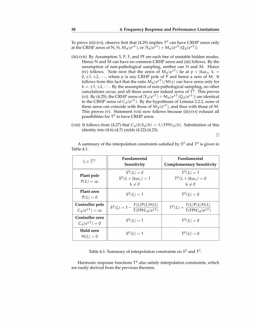
58 4. Frequency Response and Performance Limitations
To prove (iii)-(vi), observe first that (4.29) implies T0 can have CRHP zeros onlyat the CRHP zeros of N, H,Md(e
sT ), or [Yd(esT ) +Md(e
sT )Qd(esT )].
(iii)-(vii) By Assumption 3, P, F, and PF are each free of unstable hidden modes.Hence N and M can have no common CRHP zeros and (iii) follows. By theassumption of non-pathological sampling, neither can H and M. Hence(iv) follows. Note next that the zeros of Md(e
sT ) lie at p + jkωs, k =0,±1,±2, · · · , where p is any CRHP pole of P and hence a zero of M. Itfollows from this fact that the ratio Md(e
sT )/M(s) can have zeros only fork = ±1,±2, · · · . By the assumption of non-pathological sampling, no othercancelations occur, and all these zeros are indeed zeros of T0. This proves(vi). By (4.25), the CRHP zeros of [Yd(e
sT ) +Md(esT )Qd(e
sT )] are identicalto the CRHP zeros of Cd(esT ). By the hypotheses of Lemma 2.2.2, none ofthese zeros can coincide with those of Md(e
sT ), and thus with those of M.This proves (v). Statement (vii) now follows because (iii)-(vi) exhaust allpossibilities for T0 to have CRHP zeros.
(viii) It follows from (4.27) that Cd(b)Sd(b) = 1/(FPH)d(b). Substitution of thisidentity into (4.6)-(4.7) yields (4.22)-(4.23).
A summary of the interpolation constraints satisfied by S0 and T0 is given inTable 4.1.
ξ ∈ C+Fundamental Fundamental
Sensitivity Complementary Sensitivity
Plant poleS0(ξ) = 0 T0(ξ) = 1
P(ξ) =∞ S0(ξ+ jkωs) = 1 T0(ξ+ jkωs) = 0
k 6= 0 k 6= 0
Plant zeroS0(ξ) = 1 T0(ξ) = 0
P(ξ) = 0
Controller poleS0(ξ) = 1−
F(ξ)P(ξ)H(ξ)
T(FPH)d(eξT )T0(ξ) =
F(ξ)P(ξ)H(ξ)
T(FPH)d(eξT )Cd(eξT ) =∞
Controller zeroS0(ξ) = 1 T0(ξ) = 0
Cd(eξT ) = 0
Hold zeroS0(ξ) = 1 T0(ξ) = 0
H(ξ) = 0
Table 4.1: Summary of interpolation constraints on S0 and T0.
Harmonic response functions Tk also satisfy interpolation constraints, whichare easily derived from the previous theorem.

4.2 Interpolation Constraints 59
Corollary 4.2.2 (Interpolation constraints for Tk)Under the same hypotheses of Theorem 4.2.1 the following conditions are satis-fied:
(i) Tk has no poles in C+.
(ii) Let p be a pole of P with p in C+. Then
Tk(p) = 0. (4.31)
(iii) Let ζ be a zero of P with ζ in C+. Then
Tk(ζ− jkωs) = 0. (4.32)
(iv) Let γ be a zero of H with γ in C+. Then
Tk(γ− jkωs) = 0.
(v) Let a be a zero of Cd with a in DC, and am as defined in Theorem 4.2.1 (v).Then
Tk(am) = 0.
(vi) Let p be a pole of P with p in C+, and pm as defined in Theorem 4.2.1 (vi).Then
Tk(pm) =
F(pm)
F(p)ifm = −k,
0 ifm 6= −k
(4.33)
(vii) Tk has no CRHP zeros other than those given by (iii) - (vi) above.
(viii) Let b be a pole of Cd with b in DC, and bm as defined in Theorem 4.2.1 (viii).Then
Tk(bm−k) =P(bm)H(bm) F(bm−k)
T(FPH)d(b). (4.34)
Proof: Note that the harmonic functions Tk can be expressed as
Tk(s− jkωs) =F(s− jkωs)
F(s)T0(s). (4.35)
By Assumption 3, F is minimum phase and stable, so F−k/F is bistable. The resultthen follows straightforward from Theorem 4.2.1.
There are a number of differences between the interpolation constraints forthe hybrid and the continuous-time cases; we now describe these in detail.
Remark 4.2.1 (CRHP Plant Poles) Each CRHP plant pole yields constraints (4.19)directly analogous to the continuous-time case. Furthermore, each of these polesyields the additional constraints (4.21), which arise from the periodically spacedzeros of Sd(esT ) and the fact that non-pathological sampling precludes all but oneof these zeros from being canceled by a pole of P.

60 4. Frequency Response and Performance Limitations
Remark 4.2.2 (CRHP Plant Zeros) Each CRHP plant zero yields constraints (4.20)directly analogous to the continuous-time case. Note in particular that these con-straints are present independently of the choice of the hold function. The zeros ofthe discretized plant lying in DC, on the other hand, do not impose any inherentconstraints on S0. Indeed, suppose that ν ∈ DC is a zero of (FPH)d. Then for eachνk , 1
T log(ν) + jkωs, k = 0,±1,±2, · · · , it follows that
S0(νk) = 1−1
TP(νk)H(νk)Cd(ν)F(νk), (4.36)
and thus the size of S0(νk) is not independent of the choice of compensator.
Remark 4.2.3 (Unstable Compensator Poles) For analog systems, unstable plantand compensator poles yield identical constraints on the sensitivity and comple-mentary sensitivity functions; namely, when evaluated at such a pole, sensitivitymust equal zero and complementary sensitivity must equal one. Comparing (ii)and (vii) in Theorem 4.2.1, we see that in a hybrid system unstable plant andcompensator poles will generally yield different constraints on sensitivity andcomplementary sensitivity. In particular, unstable compensator poles will yieldcorresponding zeros of S0 only in special cases.
Remark 4.2.4 (Zeros of Cd) Each zero of the compensator lying inDC imposes in-finitely many interpolation constraints upon the continuous-time system becausethere are infinitely many points in the s-plane that map to the location of the zeroin the z-plane. These constraints are due to the fact that a pole at any of thesepoints will lead to an unstable discrete pole-zero cancelation.
Remark 4.2.5 (Zeros of Hold Response) By Theorem 4.2.1 (iv), zeros of H lyingin the CRHP impose constraints on the sensitivity function identical to those im-posed by CRHP zeros of the plant. A ZOH has CRHP zeros only on the jω-axis.As discussed in Chapter 3, GSHF response functions may have zeros in the openright half plane.
Remark 4.2.6 (Zeros of S0) Our list of CRHP zeros for T0 and Tk is exhaustive;however, our list for S0 is not. It is interesting to contrast this situation withthe analog case. For analog systems, the CRHP zeros of the sensitivity functionconsist precisely of the union of the CRHP poles of the plant and compensator.On the other hand, by Theorem 4.2.1 (ii) and (vii), unstable plant poles yieldzeros of S0 while unstable compensator poles generally do not. Furthermore, asthe following example shows, S0 may have CRHP zeros even if both plant andcompensator are stable.
Example 4.2.1 Consider the plant P(s) = 1/(s + 1). Discretizing with a ZOH,sample period T = 1, and no anti-aliasing filter (i.e., F(s) = 1) yields (FPH)d(z) =.6321/(z− .3670). A stabilizing discrete controller for this plant is
Cd(z) =(4.8158)(z2 + .1z+ 0.3988)
(z2 − 1.02657z+ 0.9025).

4.3 Hybrid Disturbance Rejection Properties 61
Both plant and compensator are stable; yet it may be verified that S0 has zeros ats = 0.2± j (see Figure 4.1).
00.1
0.20.3
0.40.5
0.6 0
0.5
1
−8
−7
−6
−5
−4
−3
−2
−1
x
jy/wN
log|
S0(
s)|
Figure 4.1: Fundamental sensitivity for Example 4.2.1
4.3 Hybrid Disturbance Rejection Properties
In the last section we derived a set of interpolation constraints that must be satis-fied by the hybrid sensitivity responses S0, T0, and Tk in the CRHP. As we shallsee in this section, these constraints have interpretations in terms of steady-statedisturbance rejection properties of the system. In particular, we analize periodicdisturbances of frequencies within and outside the Nyquist range, and the effectthat corresponding unstable poles of the plant and compensator have on theserejection properties. For analog systems, it is well-known that, by the internalmodel principle, an input disturbance can be asymptotically rejected if the sys-tem includes the dynamics of the disturbance [e.g., Wonham, 1985]. As we shallsee in this section, this is not generally the case for sampled-data systems.
We start analyzing those properties that are associated with unstable poles ofthe plant.
Corollary 4.3.1Assume that P has a pole at s = jω, ω ∈ ΩN. Then the steady-state response toa disturbance d(t) = ej(ω+`ωs)t, t ≥ 0,ω ∈ ΩN, ` = 0,±1,±2, . . ., is given asfollows.

62 4. Frequency Response and Performance Limitations
(i) If ` = 0, thenydss(t) = 0 . (4.37)
(ii) If ` 6= 0, then
ydss(t) = ej(ω+`ωs)t −F(j(ω+ `ωs))
F(jω)ejωt. (4.38)
Proof: By (4.9) the steady-state response is given by
ydss(t) = S0(j(ω+ `ωs))ej(ω+`ωs)t −
∞∑k=−∞k6=0
Tk(j(ω+ `ωs))ej(ω+(k+`)ωs)t
(i) By (4.19) and (4.31), S0(jω) = 0 and Tk(jω) = 0.
(ii) By (4.21), S0(j(ω + `ωs)) = 1. From (4.33) follows that Tk(j(ω + `ωs)) = 0
if k 6= −`, and T−`(j(ω+ `ωs)) = F(j(ω+ `ωs))/F(jω) if k = −`.
It follows from (4.37) that a disturbance of frequency ω ∈ ΩN will be asymp-totically rejected if the plant has a pole at jω (if necessary, the pole may be aug-mented to the plant via an analog precompensator). However, any high frequencydisturbance of frequencyω+ `ωs,ω ∈ ΩN, ` 6= 0will be passed directly throughto the output along with an alias of frequencyω whose amplitude is determinedby the ratio of the gains of the anti-aliasing filter evaluated at the two frequencies.
As pointed out in Remark 4.2.4, unstable compensator poles do not yield thesame type of constraints on S0 as the unstable poles of the plant. Moreover, unsta-ble compensator poles do not in general yield asymptotic disturbance rejection,as the following result shows.
Corollary 4.3.2Assume that Cd has a pole at z = ejωT , and that P has no poles at s = j(ω+kωs),k = 0,±1,±2, . . .. Then the steady-state response to a disturbance input d(t) =ej(ω+`ωs)t, t ≥ 0,ω ∈ ΩN, ` = 0,±1,±2, . . ., satisfies
ydss(t) = S0` (jω)ej(ω+`ωs)t −
∞∑k=−∞k6=0
Tk` (jω)ej(ω+(k+`)ωs)t, (4.39)
where
S0` (jω) = 1−P(j(ω+ `ωs))H(j(ω+ `ωs)) F(j(ω+ `ωs))
T(FPH)d(ejωT )(4.40)
and
Tk` (jω) =P(j(ω+ (k+ `)ωs))H(j(ω+ (k+ `)ωs)) F(j(ω+ `ωs))
T(FPH)d(ejωT ). (4.41)

4.3 Hybrid Disturbance Rejection Properties 63
Note that even for ` = 0 the steady-state disturbance response is in generalnonzero. For continuous-time systems, it is well known that a periodic distur-bance may be asymptotically rejected by incorporating the dynamics of the dis-turbance into the system. For a hybrid system, Corollaries 4.3.1 and 4.3.2 showthat for asymptotic disturbance rejection to be present, the dynamics should beaugmented to the plant using an analog precompensator. Including a discretizedversion of these dynamics in the digital compensator will not, in general, achievethe desired result. Exceptions to this statement may be obtained by imposingadditional structure on the hold response function.
Corollary 4.3.3Let the hypotheses of Corollary 4.3.2 be satisfied. Chooseω ∈ ΩN. Assume that
P(jω) 6= 0 (4.42)H(jω) 6= 0 (4.43)
andH(j(ω+ kωs)) = 0, for all k = ±1,±2, · · · (4.44)
Then
(i) the steady-state response to an input d(t) = ejωt, t ≥ 0 satisfies ydss(t) = 0,
(ii) the steady-state response to an input d(t) = ej(ω+`ωs)t, t ≥ 0, ` = ±1,±2, · · ·satisfies
ydss(t) = ej(ω+`ωs)t −F(j(ω+ `ωs))
F(jω)ejωt (4.45)
Proof:
(i) The steady-state response to ejωt is given by (4.9). Hypotheses (4.42)-(4.43)imply that (FPH)d(e
jωt) = 1T F(jω)P(jω)H(jω) 6= 0, and it follows from
Theorem 4.2.1 (iv) that the coefficient of ejωt in (4.9) equals one. Using(4.44) in (4.41) shows that the coefficients of the higher frequency terms in(4.9) all equal zero.
(ii) Hypotheses (4.42)-(4.44) imply that (4.40) equals one, (4.41) equals zero fork+ ` 6= 0, and that
T−`(j(ω+ `ωs)) =F(j(ω+ `ωs))
F(jω).
These facts, together with (4.39) yield (4.45).
A consequence of Corollary 4.3.3 is the well known fact that a discrete inte-grator may be used in conjunction with a ZOH to achieve asymptotic rejection ofconstant disturbances. Related results for hybrid systems with a ZOH are foundin Franklin and Emami-Naeini [1986] and Urikura and Nagata [1987]. A recent
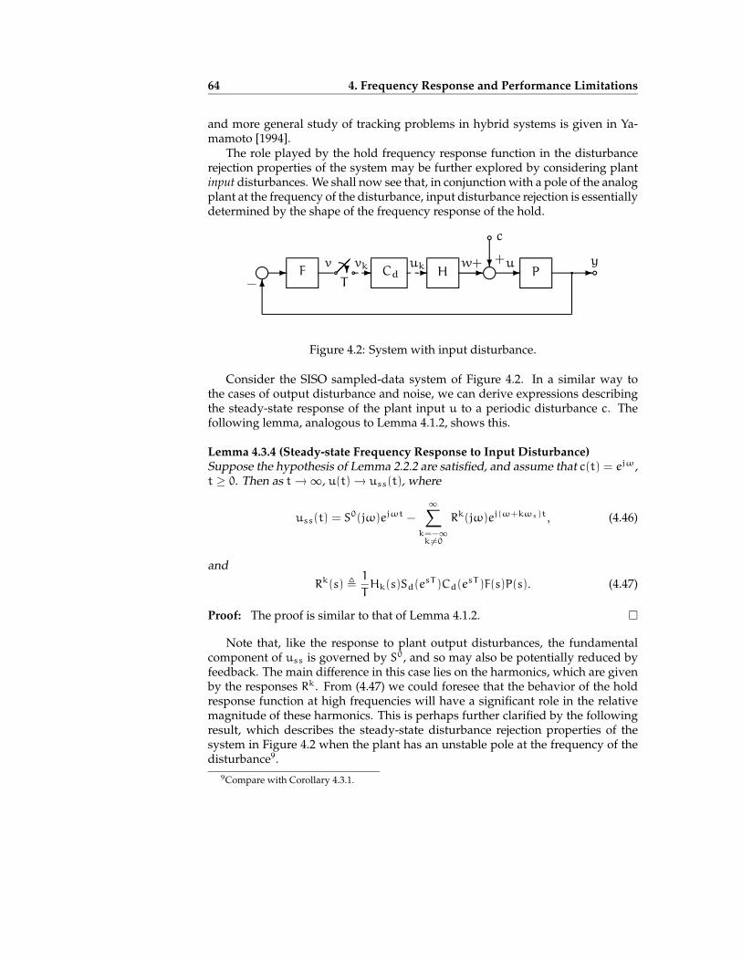
64 4. Frequency Response and Performance Limitations
and more general study of tracking problems in hybrid systems is given in Ya-mamoto [1994].
The role played by the hold frequency response function in the disturbancerejection properties of the system may be further explored by considering plantinput disturbances. We shall now see that, in conjunction with a pole of the analogplant at the frequency of the disturbance, input disturbance rejection is essentiallydetermined by the shape of the frequency response of the hold.
?i aa bi
bq- - - - --
?
6 T
y
−
ukv vk + +u
c
wF Cd H P
Figure 4.2: System with input disturbance.
Consider the SISO sampled-data system of Figure 4.2. In a similar way tothe cases of output disturbance and noise, we can derive expressions describingthe steady-state response of the plant input u to a periodic disturbance c. Thefollowing lemma, analogous to Lemma 4.1.2, shows this.
Lemma 4.3.4 (Steady-state Frequency Response to Input Disturbance)Suppose the hypothesis of Lemma 2.2.2 are satisfied, and assume that c(t) = ejω,t ≥ 0. Then as t→∞, u(t)→ uss(t), where
uss(t) = S0(jω)ejωt −
∞∑k=−∞k 6=0
Rk(jω)ej(ω+kωs)t, (4.46)
and
Rk(s) ,1
THk(s)Sd(e
sT )Cd(esT )F(s)P(s). (4.47)
Proof: The proof is similar to that of Lemma 4.1.2.
Note that, like the response to plant output disturbances, the fundamentalcomponent of uss is governed by S0, and so may also be potentially reduced byfeedback. The main difference in this case lies on the harmonics, which are givenby the responses Rk. From (4.47) we could foresee that the behavior of the holdresponse function at high frequencies will have a significant role in the relativemagnitude of these harmonics. This is perhaps further clarified by the followingresult, which describes the steady-state disturbance rejection properties of thesystem in Figure 4.2 when the plant has an unstable pole at the frequency of thedisturbance9.
9Compare with Corollary 4.3.1.

4.3 Hybrid Disturbance Rejection Properties 65
Lemma 4.3.5Assume that P has a pole at s = jω, ω in ΩN. Then the steady-state responseto an input disturbance c(t) = ej(ω+`ωs)t, t ≥ 0, ` = 0,±1,±2, . . ., is given asfollows:
(i) if ` = 0
uss(t) = −
∞∑k=−∞k 6=0
Hk(jω)
H(jω)ej(ω+kωs)t, (4.48)
(ii) if ` 6= 0
uss(t) = ej(ω+`ωs)t. (4.49)
Proof: From Lemma 4.3.4 we have that the steady-state response is given by
uss(t) = S0(j(ω+ `ω))ej(ω+`ωs)t −
∞∑k=−∞k6=0
Rk(j(ω+ `ωs))ej(ω+(k+`)ωs)t. (4.50)
(i) By the assumption of non-pathological sampling H(jω) 6= 0 holds, and socomparing (4.47) and (4.7) we may alternatively write
Rk(jω) =Hk(jω)
H(jω)T0(jω). (4.51)
Replacing (4.51) in (4.50), and applying Theorem 4.2.1 (ii) gives S0(jω) = 0
and T0(jω) = 1, from which the result follows.
(ii) Theorem 4.2.1 (vi) yields S0(j(ω + `ωs)) = 1. Since Sd(ejωT ) = 0 ands = j(ω + `ωs) could not be a pole of P by the non-pathological samplingassumption, we have that
Rk(j(ω+ `ωs)) =1
THk+`(jω)Sd(e
jωT )Cd(ejωT )F`(jω)P`(jω)
= 0.
Equation (4.49) follows.
Notice from (4.49) that harmonics are asymptotically rejected if the frequencyof the disturbance is higher than the Nyquist frequency, but the fundamentalcomponent is passed directly to the input of the plant (cf. Corollary 4.3.1).
In the case of a disturbance of frequency ω within ΩN, it follows from (4.48)that the fundamental component of the steady-state response will be asymptot-ically rejected if the plant has a pole at s = jω. However, harmonics of thisfrequency will pass with amplitudes proportional to the ratios |Hk(jω)/H(jω)|,with k = ±1,±2, . . .
In practice, the system will have acceptable asymptotic rejection propertiesif the hold frequency response rolls off at frequencies higher than the Nyquist

66 4. Frequency Response and Performance Limitations
frequency, as is the case of a ZOH10. If on the other hand the hold response islarge at high frequencies, as from Chapter 3 we know it may happen with GSHFs,harmonics at those frequencies will be amplified, thereby degrading the inputdisturbance rejection properties of the hybrid system. In addition, the presenceof these harmonics in conjunction with plant input saturation phenomena maycompromise the system’s overall performance11.
The connection between the hold response and the “size” of the steady-statesignals generated by a disturbance in case (i) of Lemma 4.3.5 is further illustratedby the following straightforward corollary. Let w denote the output of the holddevice, i.e.,
w(t) = uss(t) − c(t). (4.52)
From Lemma 4.3.5 follows that if c(t) = ejωT , and the plant has a pole at s = jω,then w is given by
w(t) =
∞∑k=−∞
Hk(jω)
H(jω)ej(ω+kωst). (4.53)
Notice that w is not necessarily periodic. However, its amplitude does corre-spond to that of a periodic function, since
|w(t)| =
∣∣∣∣∣∞∑
k=−∞Hk(jω)
H(jω)ejkωst
∣∣∣∣∣ . (4.54)
We measure the size of the steady-state value ofw by its 2-norm, over an intervalof length T . From (4.54) it follows that this is the same as
‖w‖2 =
(∫T0
|w(t)|2 dt
) 12
.
We then have the following result.
Corollary 4.3.6Assume the conditions of Lemma 4.3.5 are satisfied. Then for a disturbance c(t) =
ejωt, withω inΩN,1
T‖w‖22 =
‖h‖22|H(jω)|2
. (4.55)
Proof: From (4.53) we have that w(t)e−jωT is periodic with Fourier Series rep-resentation
w(t)e−jωT =
∞∑k=−∞
Hk(jω)
H(jω)ejkωst. (4.56)
10Notice then that the hold should have similar roll-off properties as those of the anti-aliasing filter.Further related comments are given in Chapter 5, Remark 5.2.3.
11See remarks following Lemma 3.1.2 in Chapter 3.
4.3 Hybrid Disturbance Rejection Properties 67
Application of Parseval’s Identity [e.g., Rudin, 1987] to the series (4.56) yields∫T0
|w(t)|2 dt =
∞∑k=−∞
∣∣∣∣Hk(jω)
H(jω)
∣∣∣∣2=
T‖h‖22|H(jω)|2
where in the last equality we have used Lemma 3.1.1. The result follows.
Corollary 4.3.6 shows that the “average power” of the signal generated at theoutput of the hold device by a periodic disturbance in the Nyquist range ΩN isproportional to the 2-norm of the hold pulse response h. Noting that
|H(jω)| ≤∫T0
|h(t)|dt
= ‖h‖1,
we obtain the lower bound
‖w‖2 ≥√T‖h‖2‖h‖1
. (4.57)
Since ‖h‖1 ≥√T‖h‖2, we get that ‖w‖2 ≥ 1 always. It is interesting to note that
for a ZOH ‖h‖1 =√T‖h‖2, and so it achieves the lowest bound for the size of the
signal w.We illustrate these results with a numerical example.
Example 4.3.1 (GSHF control of a harmonic oscillator) We consider Example 1in Kabamba [1987], where a GSHF is designed to stabilize the plant
P(s) =1
s2 + 1
by output feedback. The setup corresponds to the system in Figure 4.2 withF(s) = 1. This system cannot be made asymptotically stable by continuous-timedirect output feedback. However, it can be asymptotically stabilized by a digitalcompensator and a ZOH, although the closed-loop eigenvalues cannot be arbi-trarily assigned. The technique proposed by Kabamba allows the stabilizationwith just a GSHF (i.e., Cd = 1), and arbitrary closed-loop eigenvalues. The holdsuggested is a FDLTI GSHF (Definition 3.1.1) given by the matrices
K =[0 1
]L =
[0 −11 0
]M =
[−13.16827.0898
].
The sampling period selected was T = 1. This GSHF sets the closed-loop discreteeigenvalues to z = 0, so the system is stabilized in two sampling periods. Forcomparison, we alternatively computed a stabilizing solution using a ZOH and

68 4. Frequency Response and Performance Limitations
a discrete compensator. A constant compensator of gain k = −0.9348 renders adouble real pole of the discretized system at z = 0.7552.
We computed the frequency response of this GSHF using the formula givenby Lemma 3.1.5 in Chapter 3. This is plotted in Figure 4.3, together with theresponse of the ZOH for reference. We have indicated with dotted lines the ab-scissas corresponding to the frequencies ω, ω +ωs, and ω + 2ωs, where ω = 1
is the frequency of the complex poles of the plant.
GSHFZOH
0 0.5 1 1.5 2 2.5 310
−3
10−2
10−1
100
101
102
|H(jw
)|
ωΤ / 2π
ω ω+2π/Τ ω+4π/Τ
Figure 4.3: Frequency response ofGSHF and ZOH.
35 40 45 50−10
−5
0
5
10
Time
35 40 45 50−10
−5
0
5
10
Figure 4.4: Response to input distur-bance.
In reference to the summation of (4.48), we can see in this plots that the GSHFwill have a larger number of terms with significant contribution than the ZOH.Therefore, we should expect from the GSHF solution a larger steady-state re-sponse to a sinusoidal input disturbance of frequency ω = 1. This is illustratedin Figure 4.4, where we plotted the corresponding steady-state responses u forthe GSHF system (above) and for the ZOH system (below). The amplitude of thesignal produced in the GSHF case is approximately 10 times larger than that ofthe ZOH case.
4.4 Integral Relations
The interpolation constraints derived in the preceding section fix the values of thehybrid response functions at points of the CRHP. For continuous-time systems,the Poisson integral may be used to translate the interpolation constraints intoequivalent integral relations that the sensitivity and complementary sensitivityfunctions must satisfy along the jω - axis Freudenberg and Looze [1985]. In thissection, we show that similar integral relations must be satisfied by the hybridsensitivity functions. We also show that these functions must satisfy generaliza-tions of the Bode sensitivity integral Bode [1945] and its dual for complementarysensitivity Middleton and Goodwin [1990], Middleton [1991].

4.4 Integral Relations 69
4.4.1 Notation
Denote the non-minimum phase zeros of P by
ζi; i = 1, . . . ,Nζ, (4.58)
the non-minimum phase zeros of H by
γi; i = 1, . . . ,Nγ, (4.59)
the non-minimum phase zeros of Cd by
ai; i = 1, . . . ,Na (4.60)
and the ORHP poles of P by
pi; i = 1, . . . ,Np, (4.61)
including multiplicities in each case. To each ai and pi, denote the associatedNMP zeros of T0 by
aik =1
Tlog(ai) + jkωs, k = 0,±1,±2, . . . (4.62)
andpik = pi + jkωs, k = ±1,±2, . . ., (4.63)
respectively. As discussed in Chapter 3, it is possible that the hold function has acountable infinity of NMP zeros, and thus that Nγ in (4.59) equals infinity.
Denote the Blaschke products of NMP zeros of P and H by
Bζ(s) =
Nζ∏i=1
(ζi − s
ζi + s
)(4.64)
and12
Bγ(s) =
Nγ∏i=1
(γi − s
γi + s
). (4.65)
Denote the Blaschke product of ORHP plant poles by
Bp(s) =
Np∏i=1
(pi − s
pi + s
)(4.66)
For each NMP zero of Cd and for each ORHP pole of P, denote the Blaschkeproducts of associated NMP zeros of T0 by12
Bai(s) =
∞∏k=−∞
(aik − s
aik + s
)(4.67)
12That the Blaschke product (4.65) converges even if Nγ is infinite follows from Hoffman [1962].The same is valid for (4.67)-(4.68).

70 4. Frequency Response and Performance Limitations
and
Bpi(s) =
∞∏k=−∞k 6=0
(pik − s
pik + s
). (4.68)
4.4.2 Poisson Sensitivity Integral
We now derive an integral inequality that must be satisfied by log |S0(jω)|.
Theorem 4.4.1 (Poisson integral for S0)Assume that the hypotheses of Lemma 2.2.2 are satisfied. Let ξ = x + jy equalone of (4.58)-(4.59) or (4.62)-(4.63). Then∫∞
0
log |S0(jω)|Ψ(ξ,ω)dω ≥ π log|B−1p (ξ)|, (4.69)
where Ψ(s,ω) is the Poisson kernel for the half plane defined in (3.30).
Proof: Denote the NMP zeros of S0 by µ1, µ2, · · · and define the Blaschke prod-uct
Bµ(s) =∏i
µi − s
µi + s.
Then S0 = SBµ where S has no poles or zeros in the ORHP. The Poisson integral[Levinson and Redheffer, 1970, p. 225] implies that (4.69) holds with equality ifBp(ξ) is replaced by Bµ(ξ). Since the set of NMP zeros of S0 due to the ORHPpoles of P is generally a proper subset of all such zeros (cf. Remark 4.2.6) inequality(4.69) follows.
Theorem 4.4.1 has several design implications, which we describe in a seriesof remarks.
Remark 4.4.1 (NMP Plant Zeros) As in the continuous time case, if the plant isnon-minimum phase, then requiring that |S0(jω)| < 1 over a frequency range Ωimplies that, necessarily, |S0(jω)| > 1 at other frequencies. The severity of thistradeoff depends upon the relative location of the NMP zero and the frequencyrangeΩ. We now discuss this in more detail.
We recall the definition of the weighted length of an interval by the Poissonkernel for the half plane, introduced in Chapter 3, (3.35). Let ξ = x+ jy be a pointlying in C+, and consider the frequency intervalΩ = [0,ω0). Then, we had that
Θ(ξ,Ω) ,∫ω00
Ψ(ξ,ω)dω.
We have seen in Subsection 3.3.1 thatΘ(ξ,Ω) equals the negative of the phase lagcontributed by a Blaschke product of ξ at the upper end point of the interval Ω.With this notation, the following result is an immediate consequence of (4.69).

4.4 Integral Relations 71
Corollary 4.4.2Suppose that ζ = x+ jy is a NMP zero of the plant, and suppose that
|S0(jω)| ≤ α, for allω inΩ.
Then
supω>ω0
|S0(jω)| ≥ (1/α)Θ(ζ,Ω)π−Θ(ζ,Ω)
∣∣B−1p (ζ)
∣∣ ππ−Θ(ζ,Ω) (4.70)
The bound (4.70) shows that if disturbance attenuation is required throughout afrequency interval in which the NMP zero contributes significant phase lag, thendisturbances will be greatly amplified at some higher frequency. The term due tothe Blaschke product in (4.69) shows that plants with approximate ORHP pole-zero cancelations yield particularly sensitive feedback systems.
Remark 4.4.2 (NMP Hold Zeros) A non-minimum phase zero of the hold responseimposes precisely the same tradeoff as does a zero of the plant in the same loca-tion. This tradeoff is exacerbated if the NMP hold zero is near an unstable plantpole. Poor sensitivity in this case is to be expected, as an exact pole-zero cancela-tion yields an unstable hidden mode in the discretized plant13.
Remark 4.4.3 (Unstable Plant Poles) Using an analog controller, the sensitivityfunction of a system with an unstable, but minimum phase, plant can be madearbitrarily small over an arbitrarily wide frequency range Zames and Bensous-san [1983] while maintaining sensitivity bounded outside this range. This is nolonger true for digital controllers and the fundamental sensitivity function. Thefollowing result is an immediate consequence of (4.69).
Corollary 4.4.3(i) Assume that the plant has a real ORHP pole, p = x. Then
‖S0‖∞ ≥√1+
(x
ωN
)2(4.71)
(ii) Assume that the plant has an ORHP complex conjugate pole pair, p = x +jy, p = x− jy. Then for k = ±1,±2 . . .
‖S0‖∞ ≥√1+
(x
kωN
)2√1+
(x
y− kωN
)2(4.72)
13See the conditions for non-pathological sampling in Lemma 2.2.1. An example of a poorly condi-
tioned discretized system is given at the end of §7.1 in Chapter 7.

72 4. Frequency Response and Performance Limitations
Proof: We show only (i); (ii) is similar. Evaluate (4.69) with ξ equal one of (4.63),i.e., ξ = x+ jkωs, with k = ±1,±2, . . . Then
π log ‖S0‖∞ ≥∫∞0
log |S0(jω)|Ψ(ξ,ω)dω
≥ π log∣∣∣∣2x+ jkωs
−jkωs
∣∣∣∣ . (4.73)
From (4.73) follows
|S0‖∞ ≥√1+
(x
kωN
)2≥
√1+
(x
ωN
)2.
In either case of Corollary 4.4.3, the fundamental sensitivity function neces-sarily has a peak strictly greater than one.
For a real pole, achieving good sensitivity requires that the sampling ratebe sufficiently fast with respect to the time constant of the pole; e.g., achieving‖S0‖∞ < 2 requires that ωN > x/
√3. This condition is also necessary for a com-
plex pole pair. Furthermore, sensitivity will be poor if y ≈ kωN for some k 6= 0.The reason for poor sensitivity in this case is clear; if y = kωN, then the com-plex pole pair violates the non-pathological sampling condition (2.12), and thediscretized plant will have an unstable hidden mode.
More generally, we have
Corollary 4.4.4Assume that the plant has unstable poles pi and p` with pi 6= p`. Then
‖S0‖∞ ≥ maxk6=0
∣∣∣∣ pi + p` + jkωs
pi − p` − jkωs
∣∣∣∣ (4.74)
and
‖S0‖∞ ≥ maxk6=0
∣∣∣∣pi + p` + jkωs
pi − p` − jkωs
∣∣∣∣ (4.75)
It follows that if sampling is “almost pathological”, in that pi − p` ≈ jkωs, orpi − p` ≈ jkωs, then sensitivity will be large.
Remark 4.4.4 (Approximate Discrete Pole Zero Cancelations) Suppose that thediscrete compensator has an NMP zero ai. Then (4.69) holds with ξ equal to oneof the points aik (4.62) in the s-plane that map to ai in the z-plane. If the plant hasan unstable pole near one of these points, then the right hand side of (4.69) willbe large, and S0 will have a large peak. Poor sensitivity is plausible, because thissituation corresponds to an approximate pole-zero cancelation between a NMPzero of the compensator and a pole of the discretized plant.

4.4 Integral Relations 73
4.4.3 Poisson Complementary Sensitivity Integral
We now derive a result for T0 dual to that for S0 obtained in the previous section.An important difference is that we can characterize all NMP zeros of T0, and thusobtain integral equalities.
First, we note an additional property of the hold response function.
Lemma 4.4.5The hold response function (2.4) may be factored as
H(s) = H(s)e−sτHBγ(s), (4.76)
where τH ≥ 0, Bγ is given by (4.65), and log |H| satisfies the Poisson integralrelation.
Proof: Follows from Hoffman [1962, pp. 132-133].
As we discussed in Chapter 3, page 30, for a FDLTI GSHF, τH = 0. For a PCGSHF, defined by (3.11), if k denotes the smallest value of k for which ak 6= 0,then is easily seen from (3.13)-(3.14) that τH = kT/N.
We have seen in Chapter 3 explicit expressions for the zeros of a piecewiseconstant hold with α0 6= 0 and approximations to the zeros of a FDLTI hold.We remark that, in each case, H possesses infinitely many zeros which approachinfinity along well defined paths which may lie in the ORHP (See §3.2).
Theorem 4.4.6 (Poisson integral for T0)Assume that the hypotheses of Lemma 2.2.2 are satisfied. Let p` = x + jy be anORHP pole of P. Then∫∞
0
log |T0(jω)|Ψ(p`,ω)dω = πxτP + πxτH + πxNCT
+ π log |B−1ζ (p`)| + π log |B−1
γ (p`)|
+ π
Np∑i=1
log |B−1pi
(p`)| + π
Na∑i=1
log |B−1ai
(p`)|
(4.77)
where Ψ(s,ω) is the Poisson kernel for the half plane defined in (3.30).
Proof: Note that T0 has an inner-outer factorization
T0(s) = T(s) e−sτP e−sτH e−sτNCT Bζ(s)Bγ(s)
Np∏i=1
Bpi(s)
Na∏i=1
Bai(s)
where log |T | satisfies the Poisson integral Levinson and Redheffer [1970]. Sincelog |T(jω)| = log |T0(jω)|, the result follows.
We comment on the design implications of Theorem 4.4.6 in a series of re-marks.

74 4. Frequency Response and Performance Limitations
Remark 4.4.5 The first three terms on the right hand side of (4.77) show that|T0(jω)| will display a large peak if there is a long time delay in the plant, digitalcontroller, or hold function.
Remark 4.4.6 The fourth and fifth terms on the right hand side of (4.77) show that|T0(jω)| will display a large peak if there is an approximate unstable pole-zerocancelation in the plant, or between the plant and the hold function. By the non-pathological sampling condition (ii) in Lemma 2.2.1, the latter peak correspondsto an approximate unstable pole-zero cancelation in the discretized plant.
The following result is analogous to Corollary 4.4.4 for T0.
Corollary 4.4.7(i) Assume that p` = x, a real pole. Then
‖T0‖∞ ≥sinh
(πx
ωN
)(πx
ωN
) . (4.78)
(ii) Assume that p` = x+ jy, a complex pole. Then
‖T0‖∞ ≥sinh
(πx
ωN
)(πx
ωN
)∣∣∣∣∣∣∣∣sinh
(πp`
ωN
)(πp`
ωN
)∣∣∣∣∣∣∣∣∣∣∣∣∣∣∣∣(πy
ωN
)sin(πy
ωN
)∣∣∣∣∣∣∣∣ . (4.79)
Proof: By rearranging definition (4.68), we have
Bpi(s) =
∞∏k=1
1−
(pi − s
jkωs
)21−
(pi + s
jkωs
)2Using the identities [Levinson and Redheffer, 1970, p. 387],
sinπαπα
=
∞∏k=1
(1−
α2
k2
)and sin jα = j sinhα yields
Bpi(s) =
sinhπ(pi − s
ωs
)π
(pi − s
ωs
) π
(pi + s
ωs
)sinhπ
(pi + s
ωs
) (4.80)

4.4 Integral Relations 75
Note that the first factor on the right hand side of (4.80) converges to one ass→ pi. It follows that
Bp`(p`) =
(πx
ωN
)sinh
(πx
ωN
) (4.81)
Inverting yields (4.78). Furthermore
Bp`(p`) =
sin(πy
ωN
)(πy
ωN
)(πp`
ωN
)sinh
(πp`
ωN
) (4.82)
Together (4.81)-(4.82) yield (4.79).
Figure 4.5(a) give plots of the bound (4.79) versus Re p` for various valuesof Im p`, and Figure 4.5(b) give plots of the bound (4.79) versus Im p` for var-ious values of Re p`. The pole location has been normalized by the Nyquistfrequency. Note in Figure 4.5(b) that for a complex pole ‖T0‖∞ will become arbi-trarily large as y→ kωN, k = ±1,±2 . . . , because sampling becomes pathologicalat such frequencies. It follows from these plots that to achieve good robustnessthe Nyquist frequency should be chosen several times larger than the radius ofany unstable pole.
0.0
0.7
0.9
0.95
x/ω N
y/ω N
0 0.1 0.2 0.3 0.4 0.5 0.6 0.7 0.8 0.9 10
1
2
3
4
5
6
7
8
9
10
Mag
nitu
de
(a)
0.30.60.9
y/ω N
x/ω N
0 0.5 1 1.5 2 2.5 3 3.5 4 4.5 510
0
101
102
103
104
105
Mag
nitu
de
(b)
Figure 4.5: Lower bounds on ‖T0‖∞.
4.4.4 Poisson Harmonic Response Integral
Harmonic response functions (4.8) also satisfy Poisson integral relations. As forthe case of T0, in this case we also obtain an integral equality, since all the zeros of

76 4. Frequency Response and Performance Limitations
Tk in C+ are characterized. The result follows as a straightforward corollary toTheorem 4.4.6.
Corollary 4.4.8 (Poisson Integral for Tk)Assume that the hypotheses of Lemma 2.2.2 are satisfied. Let p` = x + jy be anORHP pole of P. Then∫∞0
log |Tk(jω)|Ψ(p` − jkωs,ω)dω = π log∣∣∣∣F−k(p`)
F(p`)
∣∣∣∣+ πxτP + πxτH + πxNCT
+ π log |B−1ζ (p`)| + π log |B−1
γ (p`)|
+ π
Np∑i=1
log |B−1pi
(p`)|
+ π
Na∑i=1
log |B−1ai
(p`)|
(4.83)
where Ψ(s,ω) is the Poisson kernel for the half plane defined in (3.30).
Proof: Immediately from relation (4.35),∫∞0
log |Tk(jω)|Ψ(p` − jkωs,ω)dω =
∫∞0
log∣∣∣∣ F(jω)
Fk(jω)
∣∣∣∣ Ψ(p` − jkωs,ω)dω
+
∫∞0
log |T0(j(ω+ kωs))|Ψ(p` − jkωs,ω)dω.
The first integral on the RHS of the equation above gives the first term on the RHSof (4.83), since by our assumptions on F, log(F(s)/F(s− jkωs)) satisfies a Poissonintegral relation. The second integral is the Poisson Complementary SensitivityIntegral of (4.77). The result follows.
The implications of this integral constraint are similar to those for T0, since —except for the first — all terms on the RHS of (4.83) are the same on the RHS of(4.77). Hence |Tk(jω)| will display a large peak if there are long time delays in theplant, digital controller, or hold function. There will be also large peaks if thereare approximate unstable pole-zero cancelations in the plant or between the plantand the hold function. Differently in this case, these constraints are relaxed by thepresence of the first term on the RHS of (4.83), which will be generally negativesince the anti-aliasing filter is normally designed to roll off at high frequencies.The following corollary, corresponding with Corollary 4.4.7, shows this.
Corollary 4.4.9(i) Assume that p` = x, a real pole. Then
‖Tk‖∞ ≥sinh
(πx
ωN
)(πx
ωN
) ∣∣∣∣F−k(x)
F(x)
∣∣∣∣ .
4.4 Integral Relations 77
(ii) Assume that p` = x+ jy, a complex pole. Then
‖Tk‖∞ ≥sinh
(πx
ωN
)(πx
ωN
)∣∣∣∣∣∣∣∣sinh
(πp`
ωN
)(πp`
ωN
)∣∣∣∣∣∣∣∣∣∣∣∣∣∣∣∣(πy
ωN
)sin(πy
ωN
)∣∣∣∣∣∣∣∣∣∣∣∣F−k(p`)
F(p`)
∣∣∣∣ .
4.4.5 Bode Sensitivity Integral
The following is a generalization of the classical sensitivity integral theorem ofBode [1945]. As in the case of the Poisson sensitivity integral, we only obtainan inequality, because S0 may possess NMP zeros in addition to those associatedwith ORHP plant poles.
Theorem 4.4.10Assume that the hypotheses of Lemma 2.2.2 are satisfied.
∫∞0
log |S0(jω)|dω ≥ πNp∑i=1
Re pi (4.84)
Proof: Assumption 1 implies that |sH(s)| is bounded on C+ (see (A.12) in Chap-ter A). This fact, together with the assumption that F is strictly proper, implythat
lims→∞Res≥0
|s T0(s)| = 0.
Hence the technique used in Freudenberg and Looze [1985] to derive the continuous-time version of (4.84) may be applied.
The sensitivity integral states that if |S0(jω)| < 1 over some frequency range,then necessarily |S0(jω)| > 1 at other frequencies. Hence there is a tradeoff be-tween reducing and amplifying the fundamental component of the response todisturbances at different frequencies. This tradeoff is exacerbated if the plant hasORHP poles. As in the analog cases, (4.84) does not impose a meaningful designlimitation unless an additional bandwidth constraint is imposed [e.g., Freuden-berg and Looze, 1985]. The need to prevent aliasing in hybrid systems impliesthat bandwidth constraints are potentially more severe than in the analog case.Design implications remain to be worked out, but it should be noted that the fre-quency response of the hold function as well as that of the anti-aliasing filter willneed to be considered.
4.4.6 Middleton Complementary Sensitivity Integral
We here derive an integral relation for T0 that is dual to the Bode sensitivity inte-gral obtained for S0 in the preceding section. This result is a generalization to hy-brid systems of the complementary sensitivity integral introduced in Middleton

78 4. Frequency Response and Performance Limitations
and Goodwin [1990], and Middleton [1991]. As in the case of the Poisson com-plementary sensitivity integral, exhaustive knowledge of the zeros of T0 yieldsan integral equality.
Theorem 4.4.11Assume that the hypotheses of Lemma 2.2.2 are satisfied. Suppose also thatT0(0) 6= 0. Define T0(0) = dT0/ds|s=0. Then
∫∞0
log∣∣∣∣T0(jω)
T0(0)
∣∣∣∣ dωω2 =π
2(τP + τH +NCT) + π
Nζ∑k=1
1
ζk+ π
Nγ∑k=1
1
γk− π
Np∑k=1
1
pk
+πT
2
Np∑k=1
coth(pkT
2
)+πT
2
Na∑k=1
coth(akT
2
)
+π
2
T0(0)
T0(0).
(4.85)
Proof: See §A.3 in Appendix A.
This result states that if the ratio |T0(jω)/T0(0)| < 1 over some frequencyrange, then necessarily this ratio must exceed one at other frequencies. Hence,there is a tradeoff between reducing and amplifying the fundamental componentof the response to noise in different frequency ranges. Further comments arefound in the following series of remarks.
Remark 4.4.7 The first term on the right hand side of (4.85) show that the tradeoffworsens if the plant, hold, or compensator has a time delay. The second threeterms show that the tradeoff worsens if the plant, hold, or compensator has NMPzeros. It is easy to verify that the sum of the fifth and sixth terms is positive, andthus the tradeoff also worsens if the plant has ORHP poles. For an interpretationof the seventh term, see Remark 4.4.9 below.
Remark 4.4.8 One difference between (4.85) and the analogous results in Mid-dleton and Goodwin [1990], Middleton [1991] is that the latter references assumethe presence of an integrator in the system. We avoid this requirement by insteadassuming that T0(0) 6= 0 and normalizing T0 by its DC value. This approachcould also have been taken in Middleton and Goodwin [1990], Middleton [1991];we have adopted it here to obtain a more general result. If there is indeed anintegrator in the system, then the following corollary, which follows from Corol-laries 4.3.1 and 4.3.2, shows that the normalization factor is unnecessary.
Corollary 4.4.12Assume that
(i) P contains at least one integrator, and/or

4.4 Integral Relations 79
(ii) Cd contains at least one integrator and H is a ZOH.
Then T0(0) = 1.
Remark 4.4.9 We now provide an interpretation for the ninth term in (4.85). Todo this, we consider the hybrid system depicted in Figure 4.6.
?b i aa
ibb
- - - - - -
6
-
-
6
-
r +
− T
uk uv vk
+
−y
e
1T0(0) F Cd H P
Figure 4.6: Hybrid system.
The proof of the following result is straightforward, and hence omitted.
Lemma 4.4.13Suppose that the hypotheses of Lemma 2.2.2 are satisfied.
(i) Consider the response of the system to a unit step input. Then, as t → ∞,e→ ess, where
ess(t) =
∞∑`=−∞`6=0
−P(j`ωs)H(j`ωs)
P(0)H(0)ej`ωst (4.86)
Furthermore, if H is a ZOH and/or if P contains an integrator, then ess = 0.
(ii) Consider the response of the system to a unit ramp input. Then as t → ∞,e→ ess, where
ess(t) = −T0(0)
T0(0)−
∞∑`=−∞6=0
[α` + β`t] ej`ωst, (4.87)
with
α` =d
ds
[T0(s)
T0(0)
F(s+ j`ωs)
F(s)
]∣∣∣∣s=−j`ωs
(4.88)
and
β` =P(−j`ωs)H(−j`ωs)
P(0)H(0). (4.89)
Furthermore, if H is a ZOH and/or if P contains an integrator, then β` = 0
and ess is bounded. If both these conditions are satisfied, then α` = 0 and
ess(t) = −T0(0)
T0(0). (4.90)
80 4. Frequency Response and Performance Limitations
It follows from part (ii) of Lemma 4.4.13 that the constant T0(0)/T0(0) playsa role similar to that played by the reciprocal of the velocity constant in a Type-1analog feedback system14. Hence the ninth term on the right hand side of (4.85)can ameliorate the severity of the design tradeoff only if the steady-state error toa ramp input is large and positive, so that the output lags the reference inputsignificantly.
4.5 Summary
We conclude this chapter with a brief summary of inherent design limitations forhybrid feedback systems.
Perhaps most important is the fact that those plant properties such as non-minimum phase zeros, unstable poles, and time delays that pose design diffi-culty for analog feedback systems continue to pose difficulty when the controlleris implemented digitally. Furthermore, the existence of such a difficulty is in-dependent of the type of hold function used. It is important, however, that theintersample behavior be examined if the problems are to be detected. Examiningsystem response only at the sampling instants may be misleading.
There are also a number of design limitations unique to digital controller im-plementations. First, there are limits upon the ability of high compensator gainto achieve disturbance rejection unless the hold function satisfies additional con-straints. Second, there are design limitations due to potential non-minimumphase zeros of the hold function. Perhaps most interesting are the design limi-tations due to unstable plant poles. If the sample rate is “almost pathological”and/or is slow with respect to the time constant of the pole, then sensitivity, ro-bustness, and response to exogenous inputs will all be poor.
Furthermore, as it is apparent from the results in Araki and Ito [1993], Leunget al. [1991], and Thompson et al. [1983], the fundamental and harmonic responsefunctions introduced here have connections with the L2-induced norm of the sys-tem, and therefore with its robustness properties against linear time-varying per-turbations. We shall deal with these issues in depth in the forecoming chapter.
Perhaps most interesting is the observation that the hold response functionplays a role identical to that of the anti-aliasing filter in mapping high frequencyplant behavior, including uncertainty, into the response of the discretized plant.This will be the main subject of Chapter 7.
14For an analog version of (4.90), see Truxal [1955, p. 286]

5Sensitivity Operators on L2
This chapter studies the computation of L2-induced norms of sampled-data sen-sitivity operators. The L2-induced norm is the operator norm when inputs andoutputs belong to the space of square-integrable signals L2, and it is closely re-lated to important control problems. Indeed, for LTI systems, the L2-inducednorm of a system’s operator is the H∞-norm of its transfer matrix, which repre-sents an extremely useful measure in many applications of modern control theory[e.g., Francis, 1991].
Concepts and methods associated with LTI H∞ control bear no immediateequivalent for sampled-data systems, since in this case the operators are time-varying and no transfer functions are associated with them. In view of this, con-siderable research during the last years has focused on the study of L2-norms andH∞ related problems for sampled-data systems.
Early works considering L2-norms for hybrid systems studied restricted classesof sampled-data systems Thompson et al. [1983, 1986], Chen and Francis [1990],Leung et al. [1991]. Conic sectors were applied by Thompson et al. [1983] andThompson et al. [1986] to obtain upper bounds for the L2-norm of cascade con-nections involving a sampler and a ZOH. Exact expressions for these open-loopsystems appeared later on in Chen and Francis [1990]. A formula for the L2-normof hybrid operators in a general feedback configuration was derived by Leunget al. [1991] for the case of band-limited signals.
More recent works introduced the use of lifting techniques for the H∞ analy-sis and synthesis of sampled-data systems Bamieh and Pearson [1992], Toivonen[1992], Yamamoto [1990, 1993]. As mentioned in Chapter 1, the lifting techniquetransforms the sampled-data system into a discrete time-invariant equivalent sys-tem acting over infinite-dimensional signals. Time-invariance comes as a con-sequence of periodicity, but in contrast to the classical pure discrete approach,intersample behavior is built in the model, which is reflected in the infinite di-mensionality of the transformed signals. Sampled-data H∞-norm computationand optimization Bamieh and Pearson [1992], Toivonen [1992], Yamamoto [1993],robust stabilization to LTI perturbations Dullerud and Glover [1993], and track-ing Yamamoto [1994] are some recent results obtained via lifting.
Other time-domain approaches include the formulation of an associated Hamil-tonian descriptor system Kabamba and Hara [1993], and the solution of continu-ous and discrete Riccati equations derived using the theory of linear systems with
82 5. Sensitivity Operators on L2
jumps Sivashankar and Khargonekar [1994], Sun et al. [1993], Tadmor [1991].An interesting and novel application derived from the computation of L2-
norms is the extension of the LTI concept of frequency-gain to sampled-data sys-tems Araki and Ito [1993], Araki et al. [1993], Yamamoto and Khargonekar [1996],Hagiwara et al. [1995], Yamamoto and Araki [1994]. The so-called frequency-gainof a sampled-data system is equivalent to the magnitude of a Bode plot of certaindiscrete transfer function associated with the hybrid system. In Yamamoto andKhargonekar [1996] lifting techniques were used to compute the frequency-gainof a sampled-data system. In Hagiwara et al. [1995] the same issue was addressedusing a frequency-domain framework that uses the notion of FR-operators Arakiand Ito [1993], Araki et al. [1993].
Our approach in this chapter evolves from the frequency-domain formulationintroduced in Chapter 4. In §5.1 we expound a frequency-domain lifting framework,which further exposes the harmonic structure of the sampled-data system, yield-ing a compact description of the operators that govern its behavior. This frame-work is equivalent to that of FR-operators introduced by Araki and Ito [1993]and Araki et al. [1993]. Yet, our formulation builds up on spaces of Fourier trans-forms of the original signals, while the FR-operators are defined on special spacesof time-domain signals called SD-sinusoids. The advantages of both methodsover time-domain alternatives are similar, and arise from the simplicity of thefrequency-domain description.
In §5.2 we exploit the benefits of the frequency-domain lifting to compute theL2-induced norms and frequency-gains of sampled-data sensitivity and comple-mentary sensitivity operators. Note that the complementary sensitivity opera-tor is a finite-rank operator — and therefore compact — which implies that itsnorm can be computed relatively easily. On the other hand, the sensitivity oper-ator is non-compact, which imposes a greater difficulty in the computation ofits norm Yamamoto and Khargonekar [1996]. We show that either norm andthe frequency-gains can be computed in a straightforward way from finite di-mensional discrete transfer functions. The expressions derived are easily imple-mented in numerically reliable algorithms, as we show in §5.2.2.
5.1 A Frequency-domain Lifting
Many important concepts and methods for LTI systems have no immediate ex-tension to sampled-data systems for the simple fact that sampled-data systemsare time-varying. Nevertheless, they belong to a particular class of time-varyingsystems that have a lot of structure, namely, they can be represented by periodicoperators. Most of recent advances in sampled-data control theory have beenbased on mathematical frameworks that profit from this periodic characteristic.An example of this is the time-domain lifting technique of Bamieh and Pearson[1992] and Yamamoto 1990, 1994. By lifting, a signal valued in a finite dimen-sional space is bijectively mapped into a signal valued in infinite dimensionalspaces. The great attractiveness of the transformation lies on the fact that in thenew spaces the operators are represented as LTI operators, which allow a simpler

5.1 A Frequency-domain Lifting 83
treatment of many important problems.In this section we describe a similar mathematical formalism that we call the
frequency-domain lifting1. The lifting of Bamieh and Pearson [1992] and Yamamoto[1994] is done over signals in the time-domain, which leads to state-space repre-sentations of the sampled-data system. The main difference in our approach isthat we lift signals directly in frequency-domain, which — as we shall see in theremaining sections of this chapter — may allow a simpler and more intuitivetreatment2 of problems that are naturally formulated in input-output scenarios.
Consider a signal y in the space L2(0,∞). Then, its Fourier transform Y(jω)is known to belong to L2(−∞,∞). Introduce the following sequence of functionsconstructed from Y(jω),
Yk(jω) = Y(j(ω+ kωs)), (5.1)
for ω in the Nyquist range ΩN and k integer. We arrange this sequence in aninfinite vector, and we denote it by
y(ω) ,
...Y1(jω)Y0(jω)Y−1(jω)
...
. (5.2)
We say that the infinite vector y(ω) is the — frequency-domain — lifting of thesignal Y(jω). Figure 5.1 illustrates the action of the lifting operation, which chopsup the function Y(jω) defined on (−∞,∞) into a sequence of functions Yk(jω),k = 0,±1,±2, . . . defined onΩN.
F
−2ωN−3ωN −ωN ωN
|Y(jω)|
ω
2ωN 3ωN ωN−ωN
|Y0(jω)|
2ωNωN
|Y1(jω)|
3ωN2ωN
|Y2(jω)|
ω ω ω
· · · · · ·
Figure 5.1: Action of the frequency-domain lifting operation.
Thus, y(ω) can be seen as a function defined a.e.3 over ΩN taking values in`2. Moreover, the space of such functions is a Hilbert space under the norm
‖y‖ ,(∫ΩN
‖y(ω)‖2`2dω)1/2
, (5.3)
1The concept of frequency-domain lifting is not new; it was developed in the signal processingliterature for linear discrete-time periodic systems [e.g., Shenoy et al., 1994].
2Simpler and more intuitive in the sense explained in Chapter 1, §1.2 (i).3With respect to the standard Lebesgue measure.

84 5. Sensitivity Operators on L2
and inner product
〈y, x〉 ,∫ΩN
〈y(ω), x(ω)〉`2 dω . (5.4)
We denote this space by L2(ΩN; `2) [cf. Balakrishnan, 1981]. Since the signals inL2(ΩN; `2) are basically rearrangements of signals in L2(−∞,∞), it is not difficultto see that both spaces are isomorphic with preservation of norm, as the followinglemma asserts.
Lemma 5.1.1The space L2(ΩN; `2) is isometrically isomorphic to L2(−∞,∞).
Proof: See Appendix A, §A.4.
Lemma 5.1.1 tells us that there is a bijective relation between elements inL2(−∞,∞) and elements in L2(ΩN; `2), and moreover, they have the same mea-sure, i.e.,
‖y‖L2(ΩN;`2) = ‖Y‖L2(−∞,∞).
We formalize this relationship by defining the frequency-domain lifting operator,F, mapping
F : L2(−∞,∞) → L2(ΩN; `2)
Y(jω) 7→ y(ω) .
Evidently from Lemma 5.1.1, F is invertible, and moreover, ‖F‖ = 1 = ‖F−1‖. Inparticular, if M is a bounded linear operator from L2(−∞,∞) to L2(−∞,∞), thenthe lifted operator M = F M F−1 is a bounded linear operator from L2(ΩN; `2) toL2(ΩN; `2) with the same operator norm. A key observation at this point is that itwill be in general easier and numerically more tractable to compute ‖M‖ ratherthan ‖M‖.
The representation of sampled-data operators by their liftings also revealsstructure with interesting similarities to ordinary LTI operators and their cor-responding transfer matrices. Indeed, it turns out that the lifted operator M isa multiplication operator in `2 sense, so it has an associated representation as aninfinite-dimensional “transfer matrix”. In other words, we can write (My)(ω) =Mωy(ω), where Mω is a bounded linear operator in `2 at (almost) every fixed ωin ΩN. An important consequence of this fact is that the L2-induced norm of theoperator can be computed as [cf. Yamamoto and Khargonekar, 1996]
‖M‖ = supω∈ΩN
‖Mω‖`2 , (5.5)
where ‖Mω‖`2 denotes the induced `2-norm of the operator Mω. Notice thesimilarity of (5.5) to the familiar expression of the L2-induced norm of an operatorin a LTI system, i.e., the H∞-norm of its associated transfer matrix.
In particular, we shall be concerned with compact and approximable operatorson these spaces, so we finish the section with a brief discussion of these concepts.This follows Willis [1994].

5.2 L2-induced Norms and Frequency-gains 85
Recall that a set K in a metric space is compact if each sequence in K has aconvergent subsequence. Equivalently, for any collection of open sets Vk thatcovers K, then K is compact if and only if Vk has a finite subcollection that coversK. To say that a set is compact is to say that it is “small” in some sense. The Heine-Borel Theorem [e.g., Rudin, 1987] asserts that a set in a finite-dimensional spaceis compact if and only if it is closed and bounded.
Definition 5.1.1 (Compact Operator)Let X and Y be metric spaces, and let BX denote the unit ball in X. Then theoperator T : X → Y is said to be compact if the closure of T(BX) is a compactset.
Compact operators are very close to finite-rank operators, i.e., operators whoserange is finite-dimensional. Since T(BX) is bounded if T is a bounded operator,it follows from the Heine-Borel Theorem that each finite-rank operator is com-pact. In a sense, a “converse” of this is also true in the spaces we are interestedin. Namely, a compact operator on these spaces is approximable by sequencesof finite-rank operators; i.e., if En is a sequence of finite-rank operators, thenlimn→∞ ‖En − T‖ = 0, where ‖ · ‖ denotes the induced operator norm.
5.2 L2-induced Norms and Frequency-gains
5.2.1 Sensitivity Operators
We study the sensitivity and complementary sensitivity operators for the sampled-data system of Figure 2.4. As for LTI systems, we define these operators as themappings relating output disturbance d and noise n to the output y, and denotethem respectively by
S : L2 → L2Sd 7→ y
and T : L2 → L2Tn 7→ y.
Under the assumptions of closed-loop L2-stability, S and T are bounded operatorson L2.
The actions of the sensitivity and complementary sensitivity operators are re-spectively defined in frequency-domain by the steady-state responses (4.1) and(4.2) introduced in Chapter 4, §4.1. From the definition of frequency-domain lift-ing in §5.1, it is straightforward to alternatively write (4.1) and (4.2) evaluated ats = jω in a very compact form as
y = Sωd and y = −Tωn , (5.6)
where Tω and Sω are the following infinite-dimensional transfer matrices de-fined onΩN
Tω =
. . .
......
· · · GkFk GkFk−1 · · ·· · · Gk−1Fk Gk−1Fk−1 · · ·
......
. . .
, (5.7)

86 5. Sensitivity Operators on L2
Sω =
. . .
......
· · · 1−GkFk −GkFk−1 · · ·· · · −Gk−1Fk 1−Gk−1Fk−1 · · ·
......
. . .
, (5.8)
where, to ease notation, we have omitted the explicit dependence of the variablejω in the entries of the matrices. Keep also in mind the notation Fk(jω) repre-senting F(j(ω + kωs)), which will be profusely used in the sequel. Here F(jω) isthe transfer matrix of the anti-aliasing filter, and the function G(jω) denotes theproduct
G(jω) ,1
TP(jω)H(jω)Sd(e
jωT )Cd(ejωT ) . (5.9)
Associated with F(jω) and G(jω) we define the following discretized transfermatrices that will be required to formulate our results,
Gd(ejωT ) ,
∞∑k=−∞G
∗k(jω)Gk(jω), (5.10)
and
Fd(ejωT ) ,
∞∑k=−∞ Fk(jω)F∗k(jω), (5.11)
where F∗ denotes the conjugated transpose of F. Note that if y, n, and d are valuedin Rm, then Gd(ejωT ) and Fd(ejωT ) arem×m discrete transfer matrices.
Operators Sω and Tω are infinite-dimensional transfer matrix representationsof the hybrid sensitivity and complementary sensitivity operators S and T, andverify the complementarity relation Sω + Tω = I [cf. Araki and Ito, 1993, Arakiet al., 1993, Yamamoto and Araki, 1994]. From (5.5) their induced norms are givenby
‖T‖ = supω∈ΩN
‖Tω‖`2 and ‖S‖ = supω∈ΩN
‖Sω‖`2 , (5.12)
and so, they can be evaluated by computing the functions ‖Tω‖`2 and ‖Sω‖`2 —the so-called frequency-gains of the hybrid operators [e.g., Hagiwara et al., 1995]— and then searching for suprema over the finite intervalΩN.
An important fact about the complementary sensitivity operator T is that ithas finite rank (and therefore is compact, as discussed in §5.1). We show this inthe following lemma.
Lemma 5.2.1If the inputs to the system in Figure 2.4 are valued in Rm, then T has at most rankm.
Proof: Partition F(jω) by rows, and G(jω) by columns, i.e.,
F(jω) =
f1(jω)f2(jω)
...fm(jω)
, and G(jω) =[g1(jω) g2(jω) · · · gm(jω)
].

5.2 L2-induced Norms and Frequency-gains 87
Introduce the liftings for F∗(jω) and G(jω),
f(ω) ,
...F∗1(jω)F∗0(jω)F∗−1(jω)
...
, and g(ω) ,
...G1(jω)G0(jω)G−1(jω)
...
. (5.13)
Using the partitions above, we can alternatively write
f(ω) =[f1(ω) f2(ω) . . . fm(ω)
],
andg(ω) =
[g1(ω) g2(ω) . . . gm(ω)
],
where each column fi = Ff∗i in f, and gi = Fgi in g is certainly a vector inL2(ΩN; `2), since F and G are both stable and strictly proper from our assump-tions in Chapter 2. Using this notation, the action of Tω can be alternativelywritten as
Tωn =
m∑i=1
gi〈n, fi〉`2 , (5.14)
where, 〈n, fi〉`2 is a scalar-valued function defined a.e. on ΩN4. Equation (5.14)shows that Tω is the sum ofm rank-one operators on L2(ΩN; `2). Hence it has atmost rankm, and so does T.
The fact that T is compact — and so approximable — suggests a way of nu-merically computing the norm of T by truncating Tω between harmonics −nand n, say, and evaluating the maximum singular value of the finite dimensionaltransfer matrix so obtained Araki et al. [1993]. The convergence of this sequenceof computations could be slow, though, since in generalG(jω) and F(jω) decay as1/ωp, where p is some integer depending on the relative degrees of the transfermatrices involved.
Actually, since T is of finite-rank, more efficient ways of numerically evaluat-ing the induced norm of Tω are possible and already available. Using frequency-domain techniques similar to ours, Hagiwara et al. [1995] have shown that thecomputation of the frequency-gain of a compact operator can be obtained as themagnitude of an associated discrete-time transfer matrix. For the case of ZOH,they show how to implement their procedures in a numerically reliable fashion.
The following theorem is analogous to the result of Hagiwara et al. [1995]for the case of the hybrid complementary sensitivity operator T. The patternof our proof is quite different though, and importantly, we shall use the samepattern for the more difficult case of the hybrid sensitivity operator, which is non-compact. Our results extend to the case of GSHF, and are also implementable ina numerically reliable way, as we shall see in Subsection 5.2.2.
4Often, we shall drop the dependence of the independent variable when convenient; meaning willalways be clear from context.

88 5. Sensitivity Operators on L2
We denote by λmax[M] the maximum eigenvalue of a square matrix M. Thenwe have the following result.
Theorem 5.2.2 (L2-induced Norm of the Complementary Sensitivity Operator)If the hybrid system of Figure 2.4 is L2-input-output stable, then
‖T‖2 = supω∈ΩN
λmax[Gd(e
jωT )Fd(ejωT )
]. (5.15)
Proof: Using (5.13) write Tω as a dyadic product
Tω = g(ω)f(ω)∗,
where f∗ denotes the conjugate transpose of f (i.e., f∗ is composed of “row” vec-tors of L2(ΩN, `2)). From (5.12) we have that ‖T‖ = supω∈ΩN ‖Tω‖`2 . Fix ω inΩN, and decompose `2 into
`2 = PF ⊕ P⊥F ,where PF is the subspace of `2 spanned by the range of f, and P⊥F its orthogonalcomplement. Hence, if v is a vector in P⊥F then Tωv = 0. So,
‖Tω‖`2 = supv∈`2v 6=0
‖Tωv‖`2‖v‖`2
= supv∈PFv 6=0
‖Tωv‖`2‖v‖`2
.
Vectors of `2 in PF can be finitely parameterized as
v = fα,
where α belongs to Cm, withm the number of inputs of F. Thus, we have
‖Tω‖2`2 = supα
fα6=0
α∗f∗fg∗gf∗fαα∗f∗fα
= λmax
[(f∗f)1/2(g∗g)(f∗f)1/2
]. (5.16)
Notice that both (g∗g) and (f∗f) are finitem×mmatrices, and particularly, f∗f isnon-singular since F was assumed full column rank.
Since eigenvalues are invariant under similarity transformations, (5.16) yields
‖Tω‖2`2 = λmax [(g∗g)(f∗f)] .
The proof is finished by noting that
(g∗g)(ω) = Gd(ejωT )
and(f∗f)(ω) = Fd(e
jωT )
are the discrete transfer matrices defined in (5.10) and (5.11).

5.2 L2-induced Norms and Frequency-gains 89
The case of S has to be considered more carefully, since this is a non-compactoperator, and as such, it may not be in principle approximable by sequences offinite-rank operators (which means that the norms of progressive truncations ofSω would not necessarily converge to the norm of the operator). Frequency-gains of possibly non-compact sampled-data operators have been discussed inYamamoto and Khargonekar [1996]. Their method computes the frequency-gainγω at the frequency ω by searching for the maximum value γ such that a γ-dependent generalized eigenvalue problem has an eigenvalue ejωT . Yet, the pro-cedure seems in general very hard to be implemented numerically in a reliablefashion Hagiwara et al. [1995].
The following theorem gives an expression for the frequency-gain and L2-induced norm of the hybrid sensitivity operator S. Our result relies on the factthat S verifies the complementarity relation
S = I − T,
and since T is of finite rank, it is also possible to reduce the computation of thefrequency-gain of S to a finite-dimensional eigenvalue problem. As for Theo-rem 5.2.2, these results admit a simple and reliable numerical implementation.
Theorem 5.2.3 (L2-induced Norm of the Sensitivity Operator)If the hybrid system of Figure 2.4 is L2-input-output stable, then
‖S‖2 = 1+ supω∈ΩN
λmax
[Fd(e
jωT )Gd(ejωT ) − Td(e
jωT ) −Fd(ejωT )
Td(e−jωT )Gd(e
jωT ) −Gd(ejωT ) −Td(e
−jωT )
]. (5.17)
Proof: The same idea for the proof of Theorem 5.2.2 works here. Again, for afixedω inΩN, decompose `2 into
`2 = P(F,G) ⊕ P⊥(F,G),
where P(F,G) denotes the subspace spanned by both f and g, and P⊥(F,G) its orthog-onal complement. Since Sω is block diagonal in these spaces,
‖Sω‖`2 = max
supv∈P(F,G)
v 6=0
‖Sωv‖`2‖v‖`2
, supv∈P
(F,G)⊥
v 6=0
‖Sωv‖`2‖v‖`2
= max
supv∈P(F,G)
v 6=0
‖Sωv‖`2‖v‖`2
, 1
. (5.18)
Now, any vector v in P(F,G) can be finitely parameterized as
v = fα+ gβ= [f,g]γ, (5.19)
90 5. Sensitivity Operators on L2
with γ in C2m. Denote h , [f,g], and M , h∗h. Notice that M is a finite-dimensional Hermitian matrix and, moreover, since for any vector η in C2m wehave that η∗Mη = η∗h∗hη = ‖hη‖2, M is also non-negative definite, i.e., M ≥0. Using the notation introduced in (5.10) and (5.11), and the definition of thediscrete output complementary sensitivity function (2.11) (i.e., notice that Td =f∗g), we can writeM as
M =
[Fd TdT∗d Gd
].
Introduce also the matrix N,
N ,
[Gd −I−I 0
].
It then follows that h∗(I−fg∗)(I−gf∗)h = (I+MN)M, and hence we obtain from(5.19) that
supv∈P(F,G)
v 6=0
‖Sωv‖2`2‖v‖2`2
= supγ∈C2m
γ∗Mγ+ γ∗MNMγ
γ∗Mγ
= 1+ λmax
[M1/2NM1/2
](5.20)
= 1+ λmax [MN] . (5.21)
Since in (5.21) the productMN is
MN =
[FdGd − Td −FdT∗dGd −Gd −T∗d
],
from (5.18) and (5.21) we see that it remains to show that λmax [MN] is nonnega-tive to complete the proof. This follows easily from the fact that M ≥ 0. Indeed,ifM is positive definite, i.e.,M > 0, then
δ =
[Fd TdT∗d Gd
]−1/2 [I
0
],
gives δ∗M1/2NM1/2δ = Gd ≥ 0. Thus λmax in (5.20) is nonnegative. If otherwiseM is not positive definite it is then necessarily singular, and therefore 0 must bein the spectrum ofM1/2NM1/2, which then shows that λmax [MN] ≥ 0. The proofis now complete.
Remark 5.2.1 (L2-norms and Hybrid Sensitivity Functions) As anticipated at theend of Chapter 4, the L2-induced norm of these operators may be linked to certainmeasure of the hybrid sensitivity functions S0, T0, and Tk. In fact, this connec-tion establishes that large harmonics will necessarily imply a large norm of theoperator on L2, as we shall see next. We define first the hybrid (k,m)-harmonicresponse
Tk,m , GkFm.

5.2 L2-induced Norms and Frequency-gains 91
Notice that Tk,m for k,m = ±1,±2, . . . appear as the off-diagonal entries of theinfinite-dimensional transfer matrices Tω and Sω in (5.7) and (5.8). In particu-lar, Tk,0 = Tk and T0,0 = T0, the harmonic and fundamental complementarysensitivity responses of Chapter 4. We require the following preliminary lemma.
Lemma 5.2.4Let A,B1, B2, . . . , Bk, . . . be square hermitian positive-definite matrices. Then
λmax
[∑k
BkA
]≥ max
kλmax [BkA] .
Proof:
λmax
[∑k
BkA
]= λmax
[∑k
[A12BkA
12 ]
]= maxν,‖ν‖=1
∑k
[ν∗A12BkA
12ν]
≥ maxk
maxν,‖ν‖=1
ν∗A1/2BkA1/2ν
= maxkλmax [BkA]
Now we have the following result.
Proposition 5.2.5Assume the conditions of Lemma 2.2.2 are satisfied. Then
‖T‖ ≥ maxk,m‖Tk,m‖∞
Proof: From Theorem 5.2.2,
‖T‖2 =1
T2supω∈ΩN
λmax
[(∑k
G∗kGk
)(∑m
FmF∗m
)].
Use Lemma 5.2.4 with A = (∑kG∗kGk), and Bm = FmF
∗m to get
‖T‖2 ≥ 1
T2supω∈ΩN
maxmλmax
[∑k
G∗kGkFmF∗m
],
and once more with A = FmF∗m, and Bk = G∗kGk. This yields
‖T‖2 ≥ 1
T2supω∈ΩN
maxk,m
λmax [G∗kGkFmF∗m]
= maxk,m
supω∈ΩN
‖ 1TGkFm‖22
= maxk,m‖Tk,m‖2∞.

92 5. Sensitivity Operators on L2
This result establishes that a peak in any of the harmonics will increase the L2-induced norm of T, reducing the system’s stability robustness properties againstT -periodic perturbations Sivashankar and Khargonekar [1993].
In the particular case of SISO systems, we can derive simpler formulas fromTheorems 5.2.2 and 5.2.3. The operator T is then of rank one, and so the compu-tation of its norm and the norm of S reduces to a single-eigenvalue problem.
Corollary 5.2.6If the hybrid system of Figure 2.4 is SISO, then
‖T‖ = supω∈ΩN
Φd(ejωT )|Td(e
jωT )|, (5.22)
and
‖S‖ = supω∈ΩN
1
2
(√(Φ2d(e
jωT ) − 1)|Td(ejωT )|2 + (|Sd(ejωT )| + 1)2
+
√(Φ2d(e
jωT ) − 1)|Td(ejωT )|2 + (|Sd(ejωT )| − 1)2), (5.23)
where
Φ2d(ejωT ) =
Fd(ejωT )Gd(e
jωT )
|Td(ejωT )|2. (5.24)
Proof: The proof of (5.22) follows immediately from Theorem 5.2.2. Formula(5.23) is obtained by computing λmax in (5.17) and after some algebraic manipu-lation.
The function Φd may be given some interesting interpretations that we con-sider in the following remarks.
Remark 5.2.2 (Φd as a Measure of Intersample Activity) The function Φd maybe given an interpretation as a “fidelity function”, that is, a measure of the amountof intersample behavior in the sampled-data system. Indeed, note that Φd isalways greater than or equal to 1, since by Cauchy-Schwarz
|(FPH)d(ejωT )|2 =
∣∣∣∣∣ 1T∞∑
k=−∞ Fk(jω)Pk(jω)Hk(jω)
∣∣∣∣∣2
≤
( ∞∑k=−∞ |Fk(jω)|2
)(1
T2
∞∑k=−∞ |Pk(jω)Hk(jω)|2
).
Thus, from (5.22) we can see that
‖T‖ ≤ ‖Φd‖∞‖Td‖∞,so ‖Φd‖∞ is an upper bound of the quotient between the L2-induced norms con-sidering full-time information, and sampled behavior respectively.

5.2 L2-induced Norms and Frequency-gains 93
Also notice that since Φd ≥ 1, for all ω in ΩN, then ‖T‖ ≥ ‖Td‖∞; i.e., the L2-induced norm of the discretized system gives a lower bound for the L2-inducednorm of the sampled-data system, as should be expected. The following resultformalizes this observation.
Corollary 5.2.7Under the assumptions of Corollary 5.2.6,
limΦd→1 ‖T‖ = ‖Td‖∞ (5.25)
limΦd→1 ‖S‖ = ‖Sd‖∞ (5.26)
Proof: Proof of (5.25) is immediate from (5.22). For (5.26) we have the followingfrom (5.23):
limΦd→1 ‖S‖ = lim
Φd→1 supω∈ΩN
|Sd(ejωT )| + 1+ ||Sd(e
jωT )| − 1|
2
= max‖Sd‖∞, 1= ‖Sd‖∞.
(5.27)
Hence, for example, if ‖Φd‖∞ is close to 1, then ‖T‖ ≈ ‖Td‖∞ and ‖S‖ ≈ ‖Sd‖∞,and we should expect little intersample activity.
Remark 5.2.3 (An Alignment Condition) Notice that Φd is independent of thecontroller, but depends on the prefilter, plant, and hold function. This suggestsa possibly interesting way of looking at an optimization problem; i.e., selectinga suitable discrete complementary sensitivity function Td, and then choosing theprefilter and hold to minimize Φd. In particular, when Φd = 1 the matrix onthe RHS of (5.17) becomes singular, since the vectors f and g “align”. Therefore,minimization of the intersample behavior may be interpreted as an “alignmentcondition” between the hold, plant, and prefilter. This remains as a topic forfuture investigation. Further related comments may be found in Hagiwara andAraki [1995].
5.2.2 Numerical Implementation
The expressions for the frequency-gains and L2-induced norms obtained in thelast section can be readily numerically implemented by computing Gd and Fdfrom (5.10) and (5.11). These computations can be approached as “special dis-cretizations” by considering relations similar to (2.8). In this way, the argumentsof supω∈ΩN in (5.15) and (5.17) are expressed by two rational transfer functionsin z = ejωT — the frequency-gains of the sampled-data sensitivity operators. Theinduced norms can then be computed by a straightforward search of maximaover the finite intervalΩN5.
5Similar formulas have been derived for the case of ZOH in Leung et al. [1991, Theorem 3].
94 5. Sensitivity Operators on L2
Computation of Fd(ejωT )
We compute (5.11) from the discretization Fd(z) = TZST L−1F(s)F(s) (see Fig-
ure 5.2), where F(s) denotes F(−s)T. Since F is a strictly proper rational function,the sampling of the output of FF is well-defined.
?a aT
b b- - -uk y yk
FF
Figure 5.2: Scheme to compute Fd(ejωT ).
Let a, b, c, 0 be a minimal state-space realization of F. Then, a minimal real-ization for FF is given by
A =
[a bbT
0 −aT
], B =
[0
−cT
], C =
[c 0
].
We then have the following.
Lemma 5.2.8 (Computation of Fd(ejωT ))The function Fd(ejωT ) is given by
Fd(ejωT ) = TC(ejωT I− eAT )−1B.
Proof: At the sampling instants the state response of FF is given by
xk+1 = eATxk +
∫T0
eA(T−τ)Bu(τ)dτ
= eATxk +
∫T0
eA(T−τ)Bδ(τ− T)dτuk , (5.28)
where δ is Dirac’s delta, since there is no hold device at the input of the system.From (5.28) we get the discrete system
xk+1 = Adxk + Bduk
yk = Cxk ,
where Ad = eAT and Bd = B. The result then follows from application ofLemma 2.1.2.
Computation of Gd(ejωT )
The case of Gd is slightly more complicated than the previous one, but can beapproached in a similar fashion. From (5.10) we have
Gd(ejωT ) =
∞∑k=−∞G
∗k(jω)Gk(jω)
=1
TC∗d(e
jωT )S∗d(ejωT )Ed(e
jωT )Sd(ejωT )Cd(e
jωT ),

5.2 L2-induced Norms and Frequency-gains 95
where
Ed(ejωT ) ,
1
T
∞∑k=−∞H
∗k(jω)P∗k(jω)Pk(jω)Hk(jω). (5.29)
Hence, to compute Gd we need to evaluate Ed(ejωT ). We do this by discretizingthe system depicted in Figure 5.3, i.e., the cascade of the hold H, the system PP,and the hold H. Since H is proper by definition, so is the cascade, and thereforethe sampling operation is again well-defined.
?a aTbvkb -- - - -
uk H PPy
Hu v
Figure 5.3: Scheme for computing (5.29).
Suppose that the plant P has a minimal realization a, b, c, d. Then, a minimalrealization for PP is given by
A =
[a 0
cTc −aT
], B =
[b
cTd
], C =
[dTc −bT
], D =
[dTd
]We consider the case of a FDLTI GSHF; similar derivations are also valid for a
PC GSHF. As seen in Chapter 3, a LTI GSHF is defined by a pulse response h,
h(t) =
KeL(T−t)M if t ∈ [0, T)0 otherwise
, (5.30)
for matrices K, L, and M of appropriate dimensions. The following lemma givesa formula for the computation of Ed(ejωT ) given the matrices A,B,C,D, andK, L,M.
Lemma 5.2.9 (Computation of Ed(ejωT ))The function Ed(ejωT ) in (5.29) is given by
Ed(ejωT ) = Cd(e
jωT I−Ad)Bd +Dd, (5.31)
where
Ad = eAT
Bd =
∫T0
eAτBKeLτMdτ
Cd =
∫T0
MTeLT(T−τ)KTCeAτ dτ
Dd =
∫T0
MTeLTτKTDKeLτMdτ+
∫T0
MTeLT(T−τ)KTC
∫τ0
eA(τ−σ)BKeL(T−σ)Mdσdτ

96 5. Sensitivity Operators on L2
Proof: We discretize the system of Figure 5.3 in four steps. Suppose t is in theinterval [kT, (k+ 1)T ]. First we compute the continuous-time response of the holdH to a pulse in uk. This is
u(t) = KeL((k+1)T−t)Muk. (5.32)
Second, feed u from (5.32) into PP to get
x(t) = eA(t−kT)xk +
∫t−kT0
eA(t−kT−σ)BKeL(T−σ)Mdσuk (5.33)
y(t) = Cx(t) +DKeL((k+1)T−t)Muk. (5.34)
Third, compute the response of the hold H to the output y given by (5.34) above.By Lemma 3.1.5 we know that the frequency response of the LTI GSHF is H(s) =K(sI+L)−1(eLT−e−sT )M. Let h denote the impulse response of the “conjugated”hold whose frequency response is H(s) = MT(sI−LT)−1(e−LTT−e−sT )eL
TTesTKT.Here, we neglect for the moment the “advance” of one sampling period due tothe non-causality of H, i.e., we are considering e−sT H(s) instead. It follows thenthat
h(t) =
MTeL
TtKT if t ∈ [0, T)0 otherwise
. (5.35)
We get
v(t) =
∫tkT
h(t− τ)y(τ)dτ
=
∫t−kT0
MTeLT(t−kT−τ)KTCx(τ+ kT)dτ
+
∫t−kT0
KeLT(t−kT−τ)KTDu(τ+ kT)dτ.
(5.36)
Denote the first integral on the RHS of (5.36) by v1, and the second by v2. Replacex(τ+ kT) and u(τ+ kT) in (5.36) using (5.33) and (5.32) to obtain
v1(t) =
(∫t−kT0
MTeLT(t−kT−τ)KTCeAτ dτ
)xk
+
(∫t−kT0
MTeLT(t−kT−τ)KTC
∫τ0
eA(τ−σ)BKeL(τ−σ)Mdσdτ
)uk,
(5.37)
and
v2(t) =
(∫t−kT0
MTeLT(t−kT−τ)KTDKeL(T−τ)Mdτ
)uk. (5.38)
Finally, we evaluate v = v1 + v2 at t = (k+ 1)T , which renders
xk+1 = Adxk + Bduk
vk+1 = Cdxk +Dduk,(5.39)

5.2 L2-induced Norms and Frequency-gains 97
where Ad, Bd, Cd and Dd are as claimed. To conclude, compute the Z-transformof the expressions in (5.39) above, and eliminate X to get
zV(z) = (Cd(zI−Ad)−1Bd +Dd)U(z). (5.40)
If we introduce now the advance of one sampling period neglected before, thefactor z on the RHS of (5.40) is canceled, rendering Ed(z) = V(z)/U(z) = Cd(zI−Ad)
−1Bd +Dd. Application of Lemma 2.1.2 gives the result.
Remark 5.2.4 Matrices Bd, Cd andDd in the above expressions can be easily nu-merically evaluated using matrix exponential formulas suggested by Van Loan[1978]. So, we have
Bd = [eAT 0] exp[
−A BK
0 L
]T
[0
M
],
Cd = [MT 0] exp[LT KTC
0 A
]T
[0
I
],
Dd = [MTeLT 0] exp[
−LT KTDK
0 L
]T
[0
M
]
+[MT 0] exp
LT KTC 0
0 A BK
0 0 −L
T[
0
eLTM
].
Example 5.2.1 (Sensitivity of gain-margin improvement with GSHFs) The use ofthese formulas is illustrated by computing the “frequency gain” of a system froman example in Yang and Kabamba [1994]. In this paper the authors present atechnique based on GSHFs to achieve arbitrary gain-margin improvement of afeedback system.
The plant considered in the example is the following,
P(s) =s− 2
(s− 1)(s+ 2).
Since the plant is non-minimum phase, there is a limit to the gain-margin achiev-able by LTI compensation Khargonekar et al. [1985], which in this case is 4.
Using the technique suggested by Yang and Kabamba, this plant can be stabi-lized by a FDLTI GSHF (Definition 3.1.1) determined by the matrices
K =[0 1
], L =
[0 2
1 −1
], M =
[−12616312.8194
],
and a sampling period of T = 0.05, yielding a gain-margin of 10. However, thisimprovement of gain-margin comes at the cost of a very large sensitivity to inputdisturbances. Indeed, consider the feedback loop of Figure 5.4, where we haveintroduced a plant input disturbance c. Figure 5.5 shows the frequency-gain of

98 5. Sensitivity Operators on L2
?
kb b
c-
-?
@@
-
ST
+ u+H P
c
Figure 5.4: System with plant input disturbance.
ω/ωN
Frequency Gain Discrete Sensitivity
0 0.2 0.4 0.6 0.8 110
−1
100
101
102
103
Mag
nitu
de
Figure 5.5: Hybrid frequency gains.
5.3 Summary 99
the hybrid operator on L2 mapping c to u. For comparison we also plotted thefrequency response of the discrete sensitivity function Sd.
The corresponding L2-induced norms are
‖S‖ = 134.69
‖Sd‖∞ = 1.0785,
which display a great difference. In a sense, this says that the discretized modeldoes not represent the true behavior of the system. Indeed, these norms showthat taking in account just the sampled behavior in this system gives only a veryconservative lower bound of the actual L2-gain of the hybrid system. As a conse-quence, a significant part of the system’s dynamics is “hidden” from a sampledanalysis as intersample activity. A large ‖S‖means high sensitivity to L2 plant in-put disturbances, which is particularly problematic if in addition there exist plantinput saturations. Furthermore, a large ‖S‖will also imply poor robustness prop-erties to time-varying perturbations Sivashankar and Khargonekar [1993].
5.3 Summary
This chapter has considered the hybrid sensitivity and complementary sensi-tivity operators on L2. We have described a mathematical framework called“frequency-domain lifting”, which provides a representation of these operatorsas infinite dimensional “transfer matrices”. Based on this representation we havecharacterized the frequency-gains of these operators as the maximum eigenvalueof an associated finite dimensional discrete transfer matrix. The L2-induced normof the operators is then computed by performing a search of maxima of theseeigenvalues over a finite interval of frequencies. The expressions obtained can beeasily implemented numerically to any desired degree of accuracy in a reliablefashion.
Similar expressions have been communicated in the literature for the case ofthe compact operators, like the complementary sensitivity operator [e.g., Hagi-wara and Araki, 1995]. Hybrid non-compact operators impose additional dif-ficulties in the evaluation of frequency-gains and L2-induced norms Yamamotoand Khargonekar [1993]. Perhaps most interesting in our results is the fact thatalso the sensitivity operator, which is non-compact, can be characterized as a fi-nite dimensional eigenvalue problem feasible of a numerically reliable implemen-tation.
These formulas have immediate application in the analysis of stability robust-ness for LTV unstructured perturbations, and H∞ control synthesis problems.Particularly, since our expressions allow the use of GSHFs, they provide a reli-able computational tool for the evaluation of performance of a general class ofsampled-data designs.


6Stability Robustness
Since no mathematical model can completely describe the exact behavior of aphysical system, the consideration of model uncertainty in the analysis and de-sign of feedback systems is an issue of unarguable theoretical and practical signif-icance. In this respect, one of the fundamental problems is the analysis of the sta-bility robustness of the control system, i.e., the property by which the closed-loopsystem remains stable under perturbations. This is a well-studied problem forFDLTI systems, where several useful tools, like H∞ and µ methods, have provensuccessful.
The analysis of stability robustness for sampled-data systems is more difficult,again due to their time-varying characteristics, and has attracted the attention ofa number of researchers in recent years. For example, Thompson et al. [1983]and Thompson et al. [1986] have used conic sector techniques to obtain sufficientconditions for robust stability. Similar results have been derived by Hara et al.[1991] using the L2-induced norm and the Small-gain Theorem. More recently,Sivashankar and Khargonekar [1993] have shown that the L2-induced norm ac-tually gives both necessary and sufficient conditions for robust stability when theclass of unstructured perturbations include periodic time-varying perturbations.However, as illustrated in Dullerud and Glover [1993], the L2-induced norm maybe a very conservative measure of robust stability under LTI perturbations, whichare a more natural class of uncertainties to consider since the plant is normally as-sumed LTI. Indeed, under the assumption of stable LTI perturbations, Dullerudand Glover [1993] have shown that the necessary and sufficient condition for ro-bust stability reduces to a µ type of test. This result has now been generalizedto the case of unstable perturbations by Hagiwara and Araki [1995], who usedNyquist type of arguments and the frequency-domain framework suggested inAraki and Ito [1993] and Araki et al. [1993].
The approach followed in Dullerud and Glover [1993] is based on a state-space representation of the sampled-data system, and uses time-domain liftingtechniques and a generalization of the Z-transform to obtain a representationof the operators in frequency-domain. As pointed out by Yamamoto and Khar-gonekar [1996], this detour through state-space to describe input-output opera-tors might complicate the analysis.
In this chapter, we show how these results can be obtained in a very intu-

102 6. Stability Robustness
itive and simple way — almost entirely by block-diagram manipulation — if theproblem is set up directly in frequency-domain. In §6.1 we consider stable LTImultiplicative perturbations on the analog plant. Using the frequency-domainframework introduced in Chapter 5, we derive a µ-test that corresponds with theresults of Dullerud and Glover. In the particular case of SISO systems, this testcan be reduced to an `1-type condition involving the fundamental complementarysensitivity function, T0(s), introduced in §4.1. This has an important link with theresults of Chapter 4, since it shows that peaks of T0 will have direct deleteriouseffects on the stability robustness properties of the system.
It is interesting to note that under our framework, the problem is easily broughtto the classical basic perturbation model of Figure 6.1 [see also Hagiwara and Araki,1995]. Moreover — and perhaps unsurprisingly too — we shall see that the inter-connection matrix G will be Tω, the infinite matrix representation of the sampled-data complementary sensitivity operator introduced in §5.2. Note that this is in com-plete analogy with the corresponding LTI case, where the interconnection matrixis the complementary sensitivity function [e.g., Doyle et al., 1992].
Moreover, we shall see in §6.2 that
-
−
∆G
G
Figure 6.1: Basic perturbation model.
this carries over to the problem of ro-bust stability under a divisive perturba-tion model. Again in analogy with theLTI case, this time G is Sω, the infinitematrix representation of the sampled-datasensitivity operator. The correspondingµ-test, though, will be only conjectured,since the sensitivity operator is non-compact,a fact that makes the analysis much more
intricate than the multiplicative case. Nevertheless, a necessary condition for ro-bust stability with the divisive perturbation model is easily obtained in the SISOcase. This shows that peaks in the fundamental sensitivity function S0 will nec-essarily reduce the stability margin of the hybrid system respect to this type ofperturbations.
6.1 Multiplicative Perturbation
Consider the multivariable sampled-data system depicted in Figure 6.2. The per-turbed plant is represented by the multiplicative uncertainty model
P(s) = (I+W(s)∆(s))P(s) , (6.1)
where ∆(s) is a FDLTI perturbation given by a stable rational function satisfying‖∆‖∞ < 1; we call such ∆ and admissible perturbation. The weighting functionW(s) is assumed a fixed stable, minimum-phase rational function, and such thatF(s)W(s)P(s) is proper. This type of uncertainty model is useful to represent highfrequency plant uncertainty Doyle and Stein [1981].
Assuming closed loop stability of the nominal hybrid system, i.e., for∆(s) = 0,we shall determine necessary and sufficient conditions for the perturbed systemto remain stable under the class of admissible perturbations.

6.1 Multiplicative Perturbation 103
?a a@@T
ii
-
-
-
?
-
?
+ +
v y
uk −Cd FH
P
∆ W
Figure 6.2: System with multiplicative uncertainty.
Suppose that we discretize the system of Figure 6.2 by opening the loop at theinput and output of the discrete controller Cd. Then, we obtain the simplifieddiscrete diagram of Figure 6.3, where (FPH)d is the discretized series of hold,perturbed plant and anti-aliasing filter. Applying Corollary 2.1.4 to (FPH)d yieldsthe infinite sum representation
(FPH)d(esT ) =
1
T
∞∑k=−∞ Fk(s)(I+Wk(s)∆k(s))Pk(s)Hk(s) . (6.2)
Equation (6.2) displays the multi
i
-
?−Cd
(FPH)d
Figure 6.3: Discretized perturbed system.
frequency structure induced by thesampling operation. This relation canbe translated directly into the blockdiagram of Figure 6.4. Note in thispicture that although the sampler isnot represented explicitly, its actionis structurally embedded in the blockdiagram as the parallel of an infinitenumber of direct paths where each harmonic component of the signals operates.We use this representation to derivate an expression where all the perturbations∆k are blocked together.
Take the k-harmonic direct path in Figure 6.4. Then, we can write
Vk(s) =1
TPk(s)Hk(s)Ud(e
sT ), (6.3)
where Ud is the Z-transform of the output of the controller. To ease notation, weshall drop the independent variables in the sequel of this derivation, understand-ing that all signals and transfer functions are functions of s, save for the discreteones, like Cd and Ud, which are functions of esT . Now, we have that Ud is given

104 6. Stability Robustness
h
h
h
h h h
h-
-
?-
--
?-
-
-
-
?-
- - ?
66
??
6
-
?
-
-
-
-
-
Fk1TPkHk
∆k
Cd(esT )
......
· · · · · ·++ + ++
+
+
+
+
+
+ +
......
1TP−1H−1
∆−1
F−1
1TPH F
∆ W
W−1V−1 Y−1
V Y
Vk YkWk
−
...
...
...Ud(esT )
Figure 6.4: Harmonic structure of the perturbed system.
by
Ud = −Cd
∞∑k=−∞ Fk
(WkYk +
1
TPkHkUd
)
= −Cd∑k
FkWkYk − Cd
(1
T
∑k
FkPkHk
)Ud . (6.4)
Noting that by Corollary 2.1.4 1/T∑k FkPkHk is the nominal discretized plant
(FPH)d, from (6.4) we get
Ud = −SdCd∑k
FkWkYk , (6.5)
whereSd(z) = [I+ Cd(z)(FPH)d(z))]
−1 (6.6)
is the nominal discrete Sensitivity Function. Now, replacing Ud from (6.5) andYk = ∆kVk into (6.3) yields
Vk =1
TPkHkSdCd
∑m
FmWm∆mVm . (6.7)
In the lifted domain, (6.7) can be written as
(I + TωWω∆ω) v = 0, (6.8)

6.1 Multiplicative Perturbation 105
where I is the infinite identity matrix (the identity operator in `2) and Tω is theinfinite matrix representation of the complementary sensitivity operator, definedin (5.7). Wω and ∆ω are infinite-dimensional block diagonal matrices,
Wω , diag[. . . ,Wk(jω),Wk−1(jω), . . .],
and∆ω , diag[· · · , ∆k(jω), ∆k−1(jω), · · · ],
while v is the lifted vector
v(ω) ,
...V1(ω)V0(ω)V−1(ω)
...
. (6.9)
Equation (6.8) collects system knowns and perturbations in two separatedblocks, as in the basic perturbation model of Figure 6.5. Thus, we can see clearlyin the form of∆ω how the original time-varying problem with unstructured ana-log perturbations conduces to a time-invariant, infinite-dimensional, problemwith a very structured class of perturbations. From this setup it is standard toderive the conditions for the internal stability of the loop of Figure 6.5 as a µ-test.
- ∆ω
TωWω
v−
Figure 6.5: Basic perturbation model for multiplicative uncertainty.
Before proceeding, we need to recall a few definitions relative to the struc-tured singular value µ required to state the results; we refer for example to Packardand Doyle [1993] for more details. The structured singular value of a given n×ncomplex matrix M is a nonnegative real number defined with respect to a set ∆of perturbation matrices ∆ in Cn×n of prescribed structure. Denote by σ∆ themaximum singular value of ∆. Then we define µ∆(M) as
µ∆(M) ,1
min∆∈∆
σ∆ : det(I−M∆) = 0,
unless no ∆ ∈ ∆makes (I−M∆) singular, in which case µ∆(M) , 0. The pertur-bation set ∆ is defined as the set ol perturbations ∆ of the form
∆ = diag[δ1Ir1 , δ2Ir2 , . . . , δSIrS , ∆S+1, . . . , ∆S+F], (6.10)

106 6. Stability Robustness
where δi ∈ C, ∆S+j ∈ Cmj×mj , for i = 1, 2, . . . , S, and j = 1, 2, . . . , F. With Iriwe denote Cri×ri identity matrices. Note that for dimensional consistency it isnecessary that
∑Si=1 ri +
∑Fj=1mj = n.
With these definitions, we can now state necessary and sufficient conditionsfor robust stability of the hybrid system of Figure 6.2, adapted from the result ob-tained by Dullerud and Glover [1993]. The result reduces to a µ-problem on theinfinite dimensional matrices of Figure 6.5, and it is expressed as a sequence ofall the finite dimensional µ-problems obtained by truncating the original matri-ces. Denote by [Tω]n, [Wω]n and [∆ω]n the corresponding truncations keepingall harmonics between −n and n, for some positive integer n. For each ω inΩN,[∆ω]n has a block diagonal structure, where each block ∆k(jω) is as in (6.10).Let ∆n denote the set of all these finite dimensional block diagonal matrix per-turbations, ∆n , diag[∆n, . . . , ∆−n] : ∆i ∈ ∆. Then, we have the followingproposition.
Proposition 6.1.1 (Dullerud and Glover [1993])For all ∆ such that ‖∆‖∞ < 1 the system of Figure 6.2 is internally stable if andonly if for each integer n > 0 the following inequality is satisfied
maxω∈ΩN
µ∆n([Tω]n[Wω]n) ≤ 1 . (6.11)
As mentioned before, although we started with unstructured perturbationson the analog plant, they are mapped into a very structured type of perturba-tions in the lifted space L2(`2;ΩN). In general, assuming also ∆ω unstructuredSivashankar and Khargonekar [1993] will lead to a small-gain type of test in termsof the L2-induced norm
‖TωWω‖ ≤ 1.
This small-gain condition is only sufficient for LTI perturbations, and it may bequite conservative. This has been analyzed by means of example by Dullerudand Glover [1993]. Other interesting related remarks are given in Hagiwara andAraki [1995].
A necessary condition for robust stability may be stated in terms of the fun-damental complementary sensitivity function of Chapter 4.
Theorem 6.1.2 (Necessary Condition for Robust Stability)A necessary condition for the the system of Figure 6.2 to remain stable for all ∆such that ‖∆‖∞ < 1 is that
‖T0(jω)W(jω)‖∞ ≤ 1. (6.12)
Proof: It is necessary for closed loop stability that
Sd(z) = [I+ Cd(z)(FPH)d(z)]−1 (6.13)

6.1 Multiplicative Perturbation 107
have no poles in DC. Rearranging yields
Sd(z) = [I+ Sd(z)Cd(z)(FW∆PH)d(z)]−1Sd(z). (6.14)
Since the nominal system is stable, then Sd will have no poles in DC if and only if
det[I+ Sd(ejωT )Cd(e
jωT )(FW∆PH)d(ejωT )] 6= 0 for allω. (6.15)
The proof proceeds by contradiction, following that in Chen and Desoer [1982,Theorem 2]. Denote Q(jω) , T0(jω)W(jω), and suppose that (6.12) is violated.Then there exists a frequencyω1 such that σ1 , σQ(jω1) > 1, where σ·, recall,denotes the maximum singular value. Performing a singular value decomposi-tion of Q(jω1) yields
Q(jω1) = Udiag[σ1 . . .]V∗,
where U , uij and V , vij are unitary matrices. Now assume for the momentthat there exists an admissible ∆ that also satisfies
∆(jω1) =
v11...vn1
(−σ1)−1[u∗11 . . . u∗n1
]= V diag[(−σ1)
−1, 0, . . . , 0]U∗,
(6.16)
and
∆(j(ω1 + kωs)) = 0 for k = ±1,±2, . . ., and k 6= −2ω1/ωs. (6.17)
The assumptions onW, and∆, imply that Corollary 2.1.4 may be used to calculate(FW∆PH)d. Using (6.16) and (6.17) yields
(FW∆PH)d(ejω1T ) = −
1
TF(jω1)W(jω1)V diag[−
1
σ1, 0, . . . , 0]U∗P(jω1)H(jω1),
(6.18)and therefore1
det[I+ Sd(ejω1T )Cd(e
jω1T )(FW∆PH)d(ejω1T )]
= det[I+ SdCd1
TFWV diag[(−σ1)
−1, 0, . . . , 0]U∗PH]
= det[I+ V diag[(−σ1)−1, 0, . . . , 0]U∗
1
TPHSdCdFW]
= det[I+ V diag[(−σ1)−1, 0, . . . , 0]U∗Q(jω1)]
= [I+ V diag[−1, 0, . . . , 0]V∗]
= det[V ] det[diag[0, 1, 1, . . . , 1]] det[V∗]= 0.
1We suppress dependence on the transform variable when convenient, meaning will be clear fromcontext.

108 6. Stability Robustness
Hence, (6.15) fails and so the perturbed system is unstable.It remains to show that ∆ satisfying the required properties exists. We do this
following a construction in Chen and Desoer [1982]. Consider
∆(s) ,
α1(s)...αn(s)
(−1
σ1
)fq(s)
k ′ z(s)[β1(s), . . . , βn(s)
]
where k ′ is a natural number, and
fq(s) ,ω1s
q(s2 +ω21) +ω1s, q > 0
αi(s) ,s
ω1Im vi1 + Re vi1
βi(s) , −s
ω1Im ui1 + Re ui1
z(s) ,HZOH(s− jω1)HZOH(s+ jω1)
T |HZOH(j2ω1)|η(s),
η(s) ,
(−s
ω1sin(^HZOH(j2ω1)) + cos(^HZOH(j2ω1))
),
where HZOH(s) is the frequency response function of the ZOH, and ^ denotesthe phase of a complex number. It is then straightforward to verify that
(i) ∆(jω1) satisfies (6.16) and (6.17), and
(ii) by choosing both k ′ and q large enough, ∆ is exponentially stable and, forallω 6= ±ω1, limω→∞ σ∆(jω)→ 0, i.e., ‖∆‖∞ < 1 is satisfied.
In relation to the results of Chapter 4, for SISO systems follows that if |T0(jω)|is very large at any frequency, then the hybrid system will exhibit poor robustnessto uncertainty in the analog plant at that frequency.
The necessary and sufficient condition of Proposition 6.1.1 yields an explicitexpression that also involves T0 in the SISO case. We state this in the followingcorollary.
Corollary 6.1.3 (Robust Stability Test — SISO case)If the system of Figure 6.2 is SISO, then, for all ∆ satisfying ‖∆‖∞ < 1, the systemis internally stable if and only if
∞∑k=−∞ |T0(j(ω+ kωs))W(j(ω+ kωs))| ≤ 1 for allω inΩN (6.19)
Proof: By Proposition 6.1.1, the system will be robustly stable if and only if alltruncated systems satisfy µ-condition (6.11). Fix an integer n > 0 and ω in ΩN.

6.1 Multiplicative Perturbation 109
The standard approach to evaluate µ∆n([Tω]n[Wω]n) is through the computa-tion of upper and lower bounds. Define the sets
Q , Q ∈ ∆n : Q∗Q = I (6.20)D , D ∈ ∆n : D = D∗ > 0 and D∆nω = ∆nωD for all ∆nω ∈ ∆
n . (6.21)
Then we have the following inequalities Packard and Doyle [1993]
maxQ∈Q
ρ(Q[Tω]n[Wω]n) ≤ µ∆n([Tω]n[Wω]n) ≤ infD∈D
σD[Tω]n[Wω]nD−1 .
(6.22)Note that the structure of the uncertainty in this case is diagonal,
∆nω = diag[δn(jω), . . . , δ−n(jω)],
with δi(jω) in C. As the truncated [Tω]n[Wω]n is rank-one, we can work out inclosed form the values of ρ(Q[Tω]n[Wω]n) and σD[Tω]n[Wω]nD−1 in (6.22).We show that there exist matrices Q0 and D0 such that upper and lower boundsin (6.22) coincide, yielding the expression for µ∆n([Tω]n[Wω]n). To lighten nota-tion we write in the remaining TW for [Tω]n[Wω]n.
We compute first the lower bound, i.e., the spectral radius ρ(QTW). Sincein the SISO case the complementary sensitivity operator is rank-one, so is TW,and its matrix may then be written as a dyad, i.e., in an outer product form,TW = g w∗, where the vectors
g =1
TSd Cd
PnHn
Pn−1Hn−1
...P−nH−n
and w =
F∗nW
∗n
F∗n−1W∗n−1
...F∗−nW
∗−n
.Then, QTW is also a rank-one matrix, and its only eigenvalue is λ = w∗Qg, soρ(QTW) = |w∗Qg|.
Consider the particular matrix Q0 = diag[Qn,Qn−1, . . . ,Q−n], with
Qi ,
P∗i H
∗i C∗d S∗d F∗iW∗i
|PiHi Cd Sd FiWi|if PiHi Cd Sd FiWi 6= 0
1 otherwise
Then
ρ(Q0TW) =
n∑i=−n
|PiHi Cd Sd Fi| Wi, (6.23)
and Q0 is certainly in Q.We now consider the upper bound σDTWD−1. The 2-norm of a rank-one
matrix TW = g w∗ is given by σTW = ρ(TW∗TW)1/2 = σg σw. ConsiderσD0TWD−1
0 with D0 = diag[Dn, Dn−1, . . . , D−n] and let
Di ,
∣∣∣∣ TFiWi
PiHiCdSd
∣∣∣∣1/2 if PiHiCdSdFiWi 6= 0,
1 otherwise.

110 6. Stability Robustness
Therefore,
σD0TWD−10 =
n∑i=−n
|PiHi Cd Sd FiWi| , (6.24)
with D0 in D.From (6.22), (6.23), and (6.24), we conclude that
µ∆n(QTW) =
n∑i=−n
|PiHi Cd Sd FiWi| . (6.25)
Note that (6.25) is valid for an arbitrary integer n > 0 andω inΩN.The proof is completed by recalling that
T0(s) =1
TP(s)H(s)Cd(e
sT )Sd(esT )F(s)
and using Proposition 6.1.1.
Again, as for Theorem 6.1.2, we see from this result that a large value of T0
at any frequency reduces the stability robustness properties of the system at thatfrequency. Notice that in this case the condition is an `1-type condition on thelifted vector representing T0, in contrast to that of Theorem 6.1.2, which is an`∞-type condition. Hence, for the SISO case, the condition of Theorem 6.1.2 isstraightforwardly implied by condition (6.19), since `1 ⊂ `∞.
Remark 6.1.1 This result may also be obtained dispensing with the µ-framework,in a similar way to Theorem 6.1.2. An outline of this alternative proof is providedin Appendix A, §A.5.
6.2 Divisive Perturbation
We now consider the stability robustness properties of the sampled-data systemof Figure 6.6, i.e., with a divisive type of uncertainty model. We assume that ∆andW satisfy the conditions stated in §6.1. The perturbed plant is represented by
P(s) = (I+W(s)∆(s))−1 P(s) . (6.26)
The derivation of necessary and sufficient conditions for robust stability ofthe hybrid system with this class of perturbations is considerably more difficultthan the multiplicative case, and remains as a challenging open problem. In thissection we show that the problem can be also represented by a basic perturbationmodel, where the infinite dimensional matrix Sω appears in the interconnectionmatrix. A small-gain type sufficient condition follows immediately from this rep-resentation. We also provide a necessary condition for the SISO case, that imposesa bound on the values of the fundamental sensitivity function of Chapter 4 on thejω-axis.

6.2 Divisive Perturbation 111
?a a@@Ti
i
-
?
?-
uk −
y
+ −
v
FCdH
P
W ∆
Figure 6.6: System with divisive uncertainty.
Again, we have for ∆ and W the same assumptions made for the multiplica-tive uncertainty in the previous subsection. This time, the discretized perturbedplant is given by
(FPH)d(esT ) =
1
T
∞∑k=−∞ Fk(s)(I+Wk(s)∆k(s))
−1Pk(s)Hk(s) . (6.27)
Following similar steps to those for the multiplicative case, we obtain theblock diagram of Figure 6.7 displaying the harmonic structure of the system aris-ing from the sampling process.
h h h
h
h
h
h
-
-
-
- - ?
66
??
6
-
?
-
- -
-
-
?
?
?
-
Fk1TPkHk
......
· · · · · ·+
−
+ + ++ +
......
1TP−1H−1 F−1
1TPH F
YkWk
YW
Y−1W−1
+
+
+
−
−
−
Ud(esT )
∆V
Cd(esT )
∆−1
V−1
...
...
...
∆kVk
Figure 6.7: Harmonic structure of the perturbed system with divisive uncertainty.
Based on this picture, we compute an expression analogous to (6.7) for the
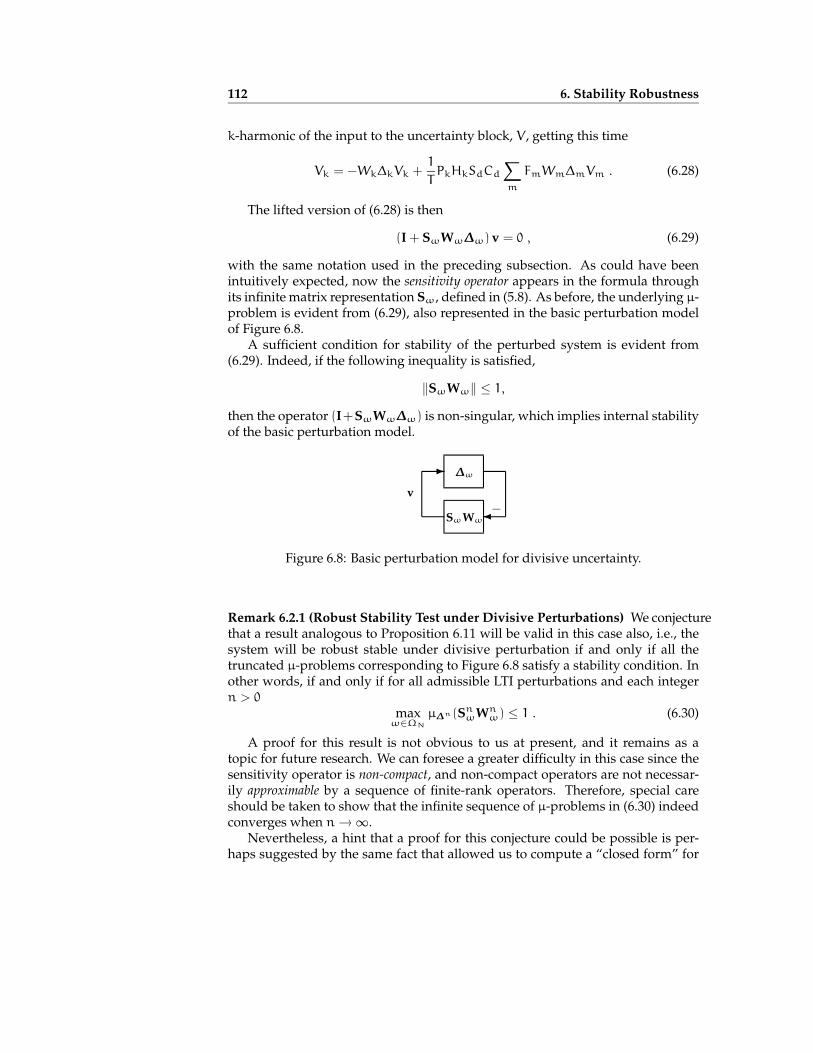
112 6. Stability Robustness
k-harmonic of the input to the uncertainty block, V , getting this time
Vk = −Wk∆kVk +1
TPkHkSdCd
∑m
FmWm∆mVm . (6.28)
The lifted version of (6.28) is then
(I + SωWω∆ω) v = 0 , (6.29)
with the same notation used in the preceding subsection. As could have beenintuitively expected, now the sensitivity operator appears in the formula throughits infinite matrix representation Sω, defined in (5.8). As before, the underlying µ-problem is evident from (6.29), also represented in the basic perturbation modelof Figure 6.8.
A sufficient condition for stability of the perturbed system is evident from(6.29). Indeed, if the following inequality is satisfied,
‖SωWω‖ ≤ 1,
then the operator (I+SωWω∆ω) is non-singular, which implies internal stabilityof the basic perturbation model.
-
SωWω
∆ω
−
v
Figure 6.8: Basic perturbation model for divisive uncertainty.
Remark 6.2.1 (Robust Stability Test under Divisive Perturbations) We conjecturethat a result analogous to Proposition 6.11 will be valid in this case also, i.e., thesystem will be robust stable under divisive perturbation if and only if all thetruncated µ-problems corresponding to Figure 6.8 satisfy a stability condition. Inother words, if and only if for all admissible LTI perturbations and each integern > 0
maxω∈ΩN
µ∆n(SnωWnω) ≤ 1 . (6.30)
A proof for this result is not obvious to us at present, and it remains as atopic for future research. We can foresee a greater difficulty in this case since thesensitivity operator is non-compact, and non-compact operators are not necessar-ily approximable by a sequence of finite-rank operators. Therefore, special careshould be taken to show that the infinite sequence of µ-problems in (6.30) indeedconverges when n→∞.
Nevertheless, a hint that a proof for this conjecture could be possible is per-haps suggested by the same fact that allowed us to compute a “closed form” for
6.3 Summary 113
the frequency-gain of this operator in Chapter 5, i.e., the sensitivity operator S isnot an arbitrary non-compact operator, since it can be written as
S = I − T,
where T is always finite-rank. Moreover, notice that a condition like (6.30) wouldin principle be valid if we impose additional restrictions on the weighting func-tion W, e.g., if it is assumed stable and strictly proper. In this case the corre-sponding infinite matrix Wω represents a compact operator, which also makesthe product SωWω compact.
A necessary condition for robust stability is easily obtained in the SISO case.In parallel with the result of Theorem 6.1.2, this condition involves the funda-mental sensitivity function S0, as we see next.
Lemma 6.2.1A necessary condition for the the system of Figure 6.6 to remain stable for all ∆such that ‖∆‖∞ < 1 is that
‖S0(jω)W(jω)‖∞ ≤ 1. (6.31)
Proof: The proof follows the same lines of that of Theorem 6.1.2 after noting thatwe can alternatively write the perturbed discrete sensitivity function as
Sd =[1+ Cd(FPH)d
]−1=
[1+ Cd(FPH)d − Cd
(F∆WPH
1+W∆ d
)]−1
=
[1− SdCd
(F∆WPH
1+W∆ d
)]−1
Sd. (6.32)
That the nonsingularity of the term between brackets in (6.32) implies (6.31) maybe shown by a contrapositive argument similar to that for the proof of Theo-rem 6.1.2, and is omitted here to avoid repetition.
In connection with the results of Chapter 4, this lemma shows that if |S0(jω)|is large at any frequency, then the system will have poor robustness to divisiveuncertainties in the analog plant at that frequency.
6.3 Summary
In this chapter we have considered the stability robustness of a hybrid system tounstructured LTI perturbations of the analog plant.
Using the frequency-domain lifting introduced in Chapter 5, we have deriveda robust stability test in the form of a structured singular value for the case of mul-tiplicative perturbations. The expression obtained was first given by Dullerudand Glover [1993] based on time-domain lifting techniques. Our procedures,
114 6. Stability Robustness
though, are considerably simplified by the use of the frequency-domain liftingtechnique.
For the case of divisive perturbations, our framework allows the problem tobe easily recasted as a basic perturbation model, from which a small-gain typesufficient condition for robust stability is directly obtained. The derivation ofnecessary and sufficient conditions for this type of perturbation model is a muchharder problem than that of multiplicative perturbations, and is left as subject ofulterior research.
For both types of perturbation models, we have drawn important connectionswith the discussion of Chapter 4 by obtaining necessary conditions for robust sta-bility of the hybrid system in terms of the fundamental sensitivity and comple-mentary sensitivity functions S0 and T0. A key conclusion of these results is thatlarge peaks in either S0 or T0 will necessarily degrade the robustness stabilityproperties of the hybrid system respect to uncertainty in the analog plant.

7An Application: DesignImplications of Discrete
Zero-placement
Non-minimum phase zeros of a linear time invariant plant impose inherent de-sign limitations that cannot be overcome by any linear time invariant controller[see Freudenberg and Looze, 1985, Middleton, 1991]. This fact suggests that moregeneral compensation schemes, such as periodic linear time-varying control, mayprove useful in controlling NMP systems. Sampled-data control, wherein an ana-log plant is controlled by a digital computer through the use of periodic sampleand hold, is one class of periodic controllers. Indeed, several authors have notedthat the zeros of a discretized plant (unlike the poles) bear no straightforward re-lationship to the zeros of the original analog plant [e.g., Kabamba, 1987, Astromand Wittenmark, 1990]. In particular, use of a GSHF with a linear time invariantdigital controller allows the zeros of the discretized plant to be placed arbitrarilyKabamba [1987], Astrom and Wittenmark [1990], Yan et al. [1994]. Hence it istempting to conclude that design limitations due to non-minimum phase zerosof an analog plant may be circumvented by assigning the zeros of the discretizedplant to be minimum phase Bai and Dasgupta [1990], Er and Anderson [1994].
On the other hand, several authors have pointed out potential disadvantagesto the use of GSHF control. In Astrom and Wittenmark [1990, p. 75] the authorsnote that “the control signal may become highly irregular”. Kabamba [1987]notes that systems with GSHF control can sometimes exhibit intersample ripple.Furthermore, Feuer and Goodwin [1994] present analyses and simulations thatsuggest that systems with GSHF controllers are prone to robustness difficultiesin addition to poor intersample behavior. Hence the potential utility of GSHFcontrol in overcoming linear time invariant design limitations is still a matter ofdebate Feuer and Goodwin [1992], Araki [1993].
We have shown in Chapter 4 that design limitations imposed by NMP zerosof the analog plant remain present when the plant is discretized using a GSHFhold, even if the discretized plant is minimum phase. In this chapter we shall providefurther interpretations to this fact by analyzing robustness properties of sampled-

116 7. Design Implications of Discrete Zero-placement
data feedback designs that rely on GSHF zero-placement capabilities.
Let us now consider a common procedure by which a digital compensator isdesigned to control an analog plant. Namely, one discretizes the plant at an ap-propriate sample rate and designs the compensator so that the discretized feed-back system has acceptable properties. As a consequence, the behavior of theanalog signals in the resulting hybrid feedback system will be acceptable at thesampling instants. One then simulates the hybrid system to verify that the inter-sample behavior is also acceptable. If the plant is discretized with a ZOH, and ifan appropriate sample rate and anti-aliasing filter are used, then this is very oftenthe case.
As noted above, an interesting feature of GSHF control is its ability to locatethe zeros of the discretized plant arbitrarily. Suppose that the analog plant hasa NMP zero within the desired closed loop bandwidth, but that the discretizedplant does not. Suppose also that the discrete closed loop system possesses feed-back properties that would be unachievable if the discretized plant also had aproblematic NMP zero. It follows as a straightforward corollary to the results ofChapter 4 that these feedback properties cannot also be present in the intersamplebehavior of the hybrid system.
A more intriguing question is whether the use of GSHF control to relocate ze-ros is responsible for sensitivity and robustness difficulties in the resulting feed-back system above and beyond those due to the NMP zero of the analog plant.It was argued in Feuer and Goodwin [1994] that the poor robustness propertiesof GSHF control are due to the way in which components of the high frequencyplant response are aliased down into the Nyquist range to form the frequencyresponse of the discretized plant. In this chapter we shall investigate this phe-nomenon in detail by developing a framework in which the robustness difficul-ties associated with zero-shifting may be studied quantitatively.
The remainder of this chapter is organized as follows. §7.1 presents a prelim-inary result that implies that the use of GSHFs to locate discrete zeros, introduceserious limitations in the continuous-time response and stabilizability propertiesof certain hybrid systems. This section motivates the more general discussion ofSections 7.2 and 7.3. In §7.2 we state and resolve the first of two Gedanken ex-periments. The first experiment shows that if one is concerned about the qualityof the intersample response, then GSHF control cannot circumvent design limita-tions due to an analog NMP zero. In §7.3 we state the second Gedanken experi-ment; unlike the first, this experiment is concerned only with performance at thesampling instants. Indeed, the analog plant enters only as a source of modelinguncertainty in the discretized system. This experiment shows that if the analogplant has at least one NMP zero with significant phase-lag contribution on theclosed-loop bandwidth of the system, then there is a tradeoff between requiring(i), high performance of the discrete system, and (ii), stability robustness withrespect to high-frequency analog plant uncertainty.

7.1 Discrete Zero-placement and ORHP Zeros of GSHFs 117
7.1 Discrete Zero-placement and ORHP Zeros of GSHFs
This section analyzes some preliminary implications of discrete zero-placementwith GSHFs. Based on a property of real pole-zero parity preservation under dis-cretization, we shall see that GSHF discrete zero-placement, as used for the strongstabilization of certain systems, will require a GSHF with zeros in the ORHP. Inview of the results of Chapters 3 and 4, these zeros may bring in stabilizabilitydifficulties and serious limitations to the continuous-time response of the hybridsystem.
Even in the case of a ZOH, a simple classification of the zeros of a discretizedsystem is not possible, except in special cases. Astrom et al. [1984] have givenasymptotic formulae for slow and fast sampling rates. Hara et al. [1989] exam-ined parity interlacing properties of real zeros and poles. The key result of theirwork is that the parity1 of the number of real zeros between any two real poles ispreserved under discretization — except possibly for cases of pathological samplingKalman et al. [1963].
At first glance, it might be expected that since GSHFs are capable of zero as-signment in the discretized plant [Bai and Dasgupta, 1990, Er and Anderson,1994, e.g.][], that no similar property holds. The proposition below, however,shows that there is a generalization of the result of Hara et al. [1989] to the caseof GSHFs.
Consider the strictly proper SISO plant P, and a GSHFH of Figure 7.1. Denoteby (PH)d the discretized plant with sampling period T ,
(PH)d(z) = ZST L−1P(s)H(s), (7.1)
where L · and Z· denote the Laplace and Z-transforms, respectively, and ST ·the sampling operation. We assume that P and H satisfy the conditions for non-pathological sampling stated in Lemma 2.2.1.
?aaT
b b-- - -
....................................................................
....................................................................
...
...
...
...
...
...
...
...
...
.
...
...
...
...
...
...
...
...
...
.
uk u
(PH)d
y ykH P
Figure 7.1: Discrete plant configuration.
Proposition 7.1.1 (Real Pole, Zero Parity Preservation in GSHF Systems)Suppose that the plant P has simple real poles at s = p1 and s = p2. Then theparity of the number of real zeros of PH on the interval (p1, p2) is the same as theparity of the number of real zeros of the discretized plant (PH)d on the interval(ep1T , ep2T ).
1Parity is even (odd) if there is an even (odd) number of zeros between the two poles.

118 7. Design Implications of Discrete Zero-placement
Before proving Proposition 7.1.1, we require the following lemma from Mid-dleton and Freudenberg [1995].
Lemma 7.1.2 (Discretized Plant by Partial Fractions Expansion)Suppose P has only simple poles, and thus let
P(s) =
n∑i=1
ri
s− pi.
Then,
(PH)d(z) =
n∑i=1
riH(pi)epiT
z− epiT.
Proof of Proposition 7.1.1: From Lemma 7.1.2,
limz→(ep1T )+
sign (PH)d(z) = sign r1H(p1)
= lims→p+
1
signP(s)H(s).
Similarly,lim
z→(ep2T )−sign (PH)d(z) = lim
s→p−2
signP(s)H(s),
from which the result follows.
Note that for the ZOH case, H has no real zeros, and so we recover the resultof Hara et al. [1989]. Also note that alteration of the zero parity of the discretizedplant — e.g., as required for strong stabilization of some systems — can only beachieved at the cost of introducing non-minimum phase zeros in the hold.
The implications of a NMP hold function in the sampled-data system are im-portant. First, it follows from the discussion in Chapter 4 that NMP zeros of thehold worsen the tradeoffs on design by adding extra limitations to the achievableanalog performance of the system. Second, and perhaps more critically, even thestabilizability properties of the system could be seriously affected by a NMP holdif its NMP zero happens to be too close to an unstable pole of the analog plant,rendering sampling “almost pathological”. This is illustrated by the followingexample.
Example 7.1.1 (Simultaneous stabilization by GSHF) In Kabamba [1987, Exam-ple 2] a FDLTI GSHF is designed to simultaneously stabilize the two systemsgiven by the transfer functions
P1(s) =1
s+ 1and P2(s) =
s− 1.5
s(s− 2), (7.2)
in the parallel configuration of Figure 7.2.

7.1 Discrete Zero-placement and ORHP Zeros of GSHFs 119
?aaT
j-
- 6
?-
+
−H
P2
P1
Figure 7.2: Simultaneous stabiliza-tion via GSHF.
.................................. .................................................................... c c6
-..................................
Im s
Re s
+∞21−1
Figure 7.3: Pole-zero map of thecombined system.
Note that the combined system,
P1(s) − P2(s) =−1.5(s− 1)
s(s+ 1)(s− 2), (7.3)
does not satisfy the conditions for strong stabilizability, namely, there is an oddnumber of positive real poles (one at s = 2) between two positive real zeros (ats = 1 and s = +∞); see Figure 7.3. Hence simultaneous stabilization is impossible[Vidyasagar, 1985, § 5.4, Corollary 12]. Following the procedures suggested byKabamba, we design a FDLTI hold with sampling time T = 1 to simultaneouslystabilize the parallel. The matrices K, L, and M corresponding to this hold weregiven in the example of Subsection 3.2.3.
1
Im z
0 ∞Re z
Figure 7.4: Discrete pole-zero map.
−2 −1.5 −1 −0.5 0 0.5 1 1.5 2−2
0
2
4
6
8
10
x
H(x
)
Figure 7.5: H on the real axis.
The discretized combined plant with this hold is
((P1 − P2)H)d(z) =(z− 0.9433)(z− 0.3641)
(z− 1)(z− e−1)(z− e2).
Notice that it is minimum phase, and so strongly stabizable. There is also onereal zero between the real poles z = e−1 and z = 1; see Figure 7.4. Hence, by

120 7. Design Implications of Discrete Zero-placement
Lemma 7.1.1, the product (P1 − P2)H will have an even number of zeros in theinterval (0, 2), and an odd number of zeros in the interval (−1, 0). By inspecting(P1 − P2) in (7.3), we conclude that H necessarily has an odd number of zeros inthose intervals. Indeed, as we see in Figure 7.5, H has zeros at s = −0.9967 ands = 0.0518.
Notice that since the NMP zero of H is very close to the open loop pole of thecontinuous plant at the origin, by Lemma 2.2.1 sampling is almost pathological,and so we should expect the discretized plant to be almost non-stabilizable/non-detectable. Indeed, this may be checked by computing the singular values of theHankel matrix for the discretized system, which are
Σ =[23163 0.1178 0.0005
].
7.2 Gedanken Experiment No. 1: Analog Performance
We have seen in the previous section that discrete zero-placement, as used insome applications of GSHF for strong stabilization, may bring in extra limitationsto the achievable analog performance of the system. In this section we broadenthis discussion by showing that if the analog plant is NMP, then the analog per-formance of the system is subject to constraints that are inescapable to GSHFsampled-data control.
Consider the following scenario. We wish to design a digital compensatorfor an analog plant having a problematic NMP zero. Suppose that a GSHF isused so that the discretized plant is minimum phase, or has NMP zeros only atless problematic locations. Then one can design a digital controller so that thediscrete sensitivity function satisfies the specification∣∣Sd(ejωT )∣∣ ≤ β1 , 0 ≤ ω ≤ ω1 (7.4)∣∣Sd(ejωT )∣∣ ≤ γ , ω1 < ω ≤ ωN, (7.5)
where β1 < 1 and γ satisfies the lower bound (C.3) imposed by the discrete Bodesensitivity integral (see Appendix C). On the other hand, the intersample behav-ior of the hybrid system must satisfy constraints due to the analog NMP zero. Wenow present a Gedanken experiment whose result shows that these constraintsmanifest themselves as limitations upon the ability of the analog response to ap-proximate that of the discretized system.
Gedanken Experiment No. 1: Suppose that we wish to design a digital con-troller for an analog plant. Then the following three questions (among others) areof interest:
(A1) Is the nominal response of the discretized system satisfactory? Equivalently,is the response of the sampled-data system satisfactory at the sampling in-stants?
7.2 Gedanken Experiment No. 1: Analog Performance 121
(A2) Does the nominal analog response approximate that of the discrete system,so that a satisfactory discrete response will correspond to satisfactory inter-sample behavior?
(A3) Is the analog response insensitive to plant uncertainty, disturbances, and sen-sor noise?
Clearly it is desirable that the answers to all three questions be affirmative. Theproposed experiment is to determine whether affirmative answers to all three of thesequestions can be obtained simultaneously.
We shall consider that the answer to (A1) is affirmative if the discrete sensi-tivity and complementary sensitivity functions are well behaved. Specifically, werequire that Sd(ejωT ) satisfy bounds of the form (7.4)-(7.5). It follows from theidentity
Sd(esT ) + Td(e
sT ) = 1 (7.6)
that if the bounds (7.4)-(7.5) are satisfied, then |Td(ejωT )| is also bounded.
To quantify the answer to (A2), define the fidelity function.
Sf(s) , S0(s) − Sd(e
sT )
= −T0(s) + Td(esT )
(7.7)
If |Sf(ejωT )| 1, then at frequency ω the fundamental component of the analog
response to disturbances, noise, and commands will closely approximate that ofthe discretized system.
Since the discrete frequency response is periodic inω, it is clearly not possible(nor desirable) that S0(jω) and T0(jω) closely approximate the discrete responsesat all frequencies. Hence we shall consider that the answer to (A2) is affirmativeif fidelity is achieved over a low frequency range:
|Sf(jω)| ≤ β2 , for 0 ≤ ω ≤ ω2 < ωN. (7.8)
Finally, as discussed in Chapter 4, it is necessary to keep the fundamentalsensitivity and complementary sensitivity functions bounded at all frequencies toprevent large intersample response to disturbances and noise, as well as to keepdifferential sensitivity from being poor. Moreover, from the results in Chapter 6(particularly Theorem 6.1.2 and Lemma 6.2.1), this is also required to preventstability robustness from being poor. Hence an affirmative answer to (A3) willrequire that S0(jω) and T0(jω) satisfy upper bounds of the form
|S0(jω)| ≤MS(ω) (7.9)
and|T0(jω)| ≤MT (ω) (7.10)
at all frequencies.It follows immediately from Theorem 4.4.1 that the analog NMP zero imposes
a limitation upon our ability to achieve affirmative answers to all of questions(A1)-(A3).

122 7. Design Implications of Discrete Zero-placement
Corollary 7.2.1Suppose that the hybrid feedback system is stable and that (7.4) and (7.8) bothhold. Defineω∗ , minω1,ω2, andΩ∗ = [0,ω∗). If the analog plant has a NMPzero at ξ, it follows that
supω>ω∗
|S0(jω)| ≥(
1
β1 + β2
) Θ(ξ,Ω∗)π−Θ(ξ,Ω∗) ∣∣B−1
p (ξ)∣∣ ππ−Θ(ξ,Ω∗) , (7.11)
where Bp is the Blaschke product of the unstable poles of the plant (cf. Subsec-tion 4.4.1), and Θ(ξ,Ω∗) is the weighted length of the interval Ω∗, defined inChapter 3, (3.35).
Proof: It follows as a direct application of Corollary 4.4.2, taking into accountbounds (7.4) and (7.8).
The peak in |S0(jω)| associated with making both β1 and β2 small will tend toviolate the bounds (7.9)-(7.10) unless ω∗ is sufficiently small that the NMP zerodoes not contribute significant phase lag at this frequency.
7.3 Gedanken Experiment No. 2: Discrete Response
We argued in the preceding section that GSHF control is ineffective at removingthe design limitations due to analog NMP zeros. Indeed, there exists a tradeoffbetween the quality of the response at sampling instants and that of the inter-sample behavior. Specifically, if |Sd(e
jωT )| is made small over a wide frequencyband relative to the location of the NMP zero, then |S0(jω)| cannot closely ap-proximate the discrete response over this band without incurring large peaks athigher frequencies.
In the present section, we shall argue that use of GSHF control to shift zerosso that the discrete sensitivity function can be made small over a wide frequencyrange may lead to unacceptable robustness difficulties even if no requirement isimposed upon the analog response. The source of these difficulties is the necessity tomaintain stability robustness against the contribution of high frequency aliases tothe discrete plant response.
7.3.1 Formulation of Gedanken Experiment No. 2
Consider the formula (2.9), which shows that the response of the discretized plantat a frequency ω ∈ ΩN depends upon the response of the analog plant, prefilter,and hold function at infinitely many frequenciesω+ kωs, k = 0,±1,±2, . . .
To explore this phenomenon further, let us rewrite (2.9) as
(FPH)d(esT ) =
1
TF(s)P(s)H(s) +
1
TΥ(s), (7.12)
whereΥ(s) ,
∑k 6=0
Fk(s)Pk(s)Hk(s). (7.13)

7.3 Gedanken Experiment No. 2: Discrete Response 123
It follows from (7.12)-(7.13) that if for some value of s the analog plant hasa zero, P(s) = 0, but the discretized plant does not, (FPH)d(e
sT ) 6= 0, then nec-essarily the response of the discretized plant at z = esT must depend upon theresponse of the analog plant at one or more of the frequencies s+ jkωs, k 6= 0. Asa corollary, the response of the discretized system will be potentially sensitive touncertainty in the analog plant at these frequencies. This fact is significant in thatuncertainty in the plant model generally increases at higher frequencies. Henceif a strong dependence upon high frequency plant behavior is required to shift azero, then one might suspect that the sensitivity and robustness of the resultingdesign would be poor. We now propose another Gedanken experiment whoseresult should serve to clarify this issue.
Gedanken Experiment No. 2: Suppose that we wish to design a digital con-troller for an analog plant. Then the following two questions (among others) areof interest:
(D1) Is the nominal response of the discrete system satisfactory?
(D2) Is the discrete response insensitive to uncertainty in the analog plant?
Clearly, it is desirable that the answers to both questions be affirmative. The pro-posed experiment is to determine whether affirmative answers to both of these questionscan be obtained simultaneously.
Note that we are now concerned solely with the response of the system atthe sampling instants and are imposing no requirement that the nominal or robustintersample behavior be satisfactory. The only requirement concerning the analogsystem is that the behavior at sampling instants be robust against uncertainty inthe analog plant.
Let us now revisit the problem of achieving robust stability against linear timeinvariant uncertainty in the analog plant. Motivated by the discussion surround-ing (7.12)-(7.13), we shall consider separately uncertainty in the two terms on theright hand side of (7.12). In particular since uncertainty in the analog plant tendsto increase with frequency, it follows that for ω ∈ ΩN uncertainty in the termF(jω)P(jω)H(jω) will tend to be dominated by uncertainty in the term Υ(jω)due to the high frequency aliases.
Consider uncertainty in the discretized plant due to analog plant uncertaintyof the form
P(s) = P(s) (1+W(s)∆(s)) , (7.14)
where ∆ is stable and proper, with |∆(jω)| < 1 for all ω, and W is a stable, min-imum phase weighting function used to represent frequency dependence of themodeling error. A necessary and sufficient condition for the sampled-data sys-tem to remain stable under uncertainty of the form (7.14) was derived in Dullerudand Glover [1993], and was discussed in Chapter 6. This condition concerns aninfinite sequence of µ-tests, but in the case of SISO systems simplifies to the ex-

124 7. Design Implications of Discrete Zero-placement
pression
supω∈ΩN
∞∑k=−∞ |T0k (jω)Wk(jω)| ≤ 1, (7.15)
as we stated in Corollary 6.1.3. We have also seen in Chapter 6, Theorem 6.1.2,that a necessary condition for robust stability was
|T0(jω)W(jω)| ≤ 1 for allω in R. (7.16)
Typically, |W(jω)| becomes unbounded at high frequencies, and thus it is neces-sary that |T0(jω)| → 0 sufficiently rapidly as ω → ∞. An inspection of the proofof this result in Chapter 6 reveals that the effects of aliases in (7.12) are ignoredin deriving (7.16). We now develop a stronger necessary condition that does takealiases into account. Define
w = infω6∈ΩN
|W(jω)|. (7.17)
Then, we have the following.
Corollary 7.3.1A necessary condition for robust stability of the sampled-data system is that
|T0(jω)W(jω)| +w|Sf(jω)| ≤ 1, for allω inΩN. (7.18)
Proof: It follows immediately from (7.15) and (7.7), since∑k
|T0k(jω)Wk(jω)| ≥ |T0(jω)W(jω)|
+w
T
∑k 6=0
|Fk(jω)Pk(jω)Hk(jω)Sd(ejωT )Cd(e
jωT )|
≥ |T0(jω)W(jω)| +w|Sf(jω)|.
Since relative uncertainty in the analog plant (7.14) typically becomes large athigh frequencies, and since the Nyquist frequency is usually chosen to be around5 times the desired closed loop bandwidth, it is not unreasonable to assume thatw in (7.17) is greater than 1. Hence (7.18) requires that |Sf(jω)| < 1 over theNyquist range. This fact is significant since, as we shall see in the next subsection,Sf must satisfy a Poisson integral relation.
7.3.2 Interpolation Constraints and an Integral Relation
We now state a set of interpolation constraints and an integral relation that mustbe satisfied by the fidelity function, Sf. We first require an additional assumptionthat will hold generically.

7.3 Gedanken Experiment No. 2: Discrete Response 125
Assumption 5If ξ is a CRHP zero of P or H, then eξT is not a zero of (FPH)d.
Proposition 7.3.2 (Interpolation Constraints for the Fidelity Function)Suppose that the sampled-data feedback system is stable, and that P, F,H, and Cdsatisfy all assumptions stated in Chapter 2 as well as Assumption 5. Then thefollowing conditions are satisfied:
(i) Let ζ be a CRHP zero of P. Then
Sf(ζ) = Td(eζT ). (7.19)
(ii) Let γ be a CRHP zero of H. Then
Sf(γ) = Td(eγT ). (7.20)
(iii) Let a be a zero of Cd with a ∈ DC. Define
ak ,1
Tlog(a) + jkωs, with k = 0,±1,±2, . . .. (7.21)
ThenSf(ak) = 0, for all k. (7.22)
(iv) Let p be a CRHP pole of P. Define
pk , p+ jkωs, with k = ±1,±2, . . .. (7.23)
ThenSf(p) = 0 and Sf(pk) = 1 (7.24)
(v) Let δ be a CRHP zero of Υ. Then
Sf(δ) = 0. (7.25)
(vi) Sf has no CRHP zeros other than those given in (iii), (iv), and (v).
Proof: From (7.7) and (7.13) we can alternatively write
Sf(s) =1TΥ(s)
(FPH)d(esT )Td(e
sT ). (7.26)
Conditions (i) and (ii) follow then from Assumption 5, and the identity (7.26).Condition (iii) follows from the identity
Sf(s) =1
TΥ(s)Sd(e
sT )Cd(esT ). (7.27)
Condition (iv) follows from (7.26). Condition (v) follows from (7.27). Finally,(7.27) shows that the zeros of Sf are restricted to those of Υ(s), Sd(esT ), andCd(e
sT ), and condition (vi) follows.

126 7. Design Implications of Discrete Zero-placement
These interpolation constraints fix the values of the fidelity function at somepoints of the CRHP. As we have seen in Chapter 4, the Poisson integral may beused to translate the interpolation constraints into an equivalent integral relation.The following result shows this.
Theorem 7.3.3 (Poisson Integral for the Fidelity Function)Let ξ = x+ jy equal one of the NMP zeros of P or H. Then∫∞
0
log |Sf(jω)|Ψ(ξ,ω)dω ≥ π log∣∣Td(eξT )∣∣ (7.28)
where Ψ(ξ,ω) is the Poisson kernel for the half plane defined in (3.30).
Proof: Note that we can write
Sf(s) = Sf(s)Bp(s)Ba(s)Bρ(s)Bδ(s)e−sτ∆e−sNcT ,
where Sf satisfies the Poisson integral relation Hoffman [1962], and2
Bp is the Blaschke product of the poles of P in C+,Ba is the Blaschke product of the poles of Cd(esT ) in C+,Bρ is the Blaschke product of the poles of (FPH)d(e
sT ) in C+, andBδ is the Blaschke product of the zeros of Υ in C+.
This fact, together with the identities |Sf(jω)| = |Sf(jω)| and Sf(ξ) = Td(ξ), yieldthe desired results.
The integral (7.28) imposes a constraint upon values of |Sf(jω)|. Analysis ofdesign implications is deferred to the next section.
7.3.3 Result of Gedanken Experiment No. 2
Suppose that the analog plant has at least one NMP zero and is subject to largemodeling uncertainty at high frequencies. Using the Poisson integrals for Sd(ejωT )(see Appendix C), and Sf(jω) given by (7.28), we now show that there exists alimitation upon the ability of a sampled-data feedback system to satisfy, with af-firmative answers, questions (D1) and (D2) of this Gedanken experiment. Specif-ically, we shall show that there exists a tradeoff between requiring (i) high per-formance in the discrete system and (ii) stability robustness with respect to theanalog plant uncertainty. The severity of this tradeoff is determined by the rel-ative location of the analog NMP zero, and is independent of whether or not thediscretized plant is minimum phase. Furthermore, the tradeoff exists even if no per-formance requirements are imposed upon intersample behavior.
We shall state performance requirements in terms of bounds upon the discretesensitivity function:
|Sd(ejωT )| ≤ β, for allω inΩε , [0, εωN) (7.29)
|Sd(ejωT )| ≤ γ, with εωN < ω ≤ ωN, for ε < 1, (7.30)
2Compare with Subsection 4.4.1 in Chapter 4.

7.3 Gedanken Experiment No. 2: Discrete Response 127
where β < 1, and γ satisfies the lower bound γ > (1/β)ε/(1−ε) imposed by thediscrete version of the Bode sensitivity integral, (C.3) in Appendix C.
If the discretized plant is minimum phase, then any such specification can beachieved. Note that the bounds (7.29)-(7.30) imply that |Td(e
jωT )| is also bounded.We now show that requiring Sd(ejωT ) to satisfy bounds such as (7.29)-(7.30) im-poses constraints upon the values of Td(esT ) off the unit circle.
Lemma 7.3.4Assume that Sd is stable and that Sd(ejωT ) satisfies the bounds (7.29)-(7.30). Con-sider ν = eξT , where ξ ∈ ORHP. Then
|Td(eξT )| ≥ FT (ξ, β, γ, ε), (7.31)
where
FT (ξ, β, γ, ε) , 1− βΘd(ξ,Ωε)
π γπ−Θd(ξ,Ωε)
π (7.32)
Proof: It follows from Corollary C.1.4 in Appendix C that
|Td(eξT ) − 1| ≤ β
Θd(ξ,Ωε)π γ
π−Θd(ξ,Ωε)π |Bξ(e
ξT )|, (7.33)
from which the result follows.
This result shows that if the specification imposed upon |Sd(ejωT )| is very strin-
gent (i.e., if β 1) then the lower bound on |Td(eξT )| will nearly equal one.
Proximity to one is determined by the relative location of the zero with respectto the interval Ωε. This point is illustrated for a real zero, ξ = x, in Figure 7.6,wherein we plot FT (ξ, β, γ, ε) vs. the ratio x/εωN for γ = 2, ε = 0.2, and variousvalues of β. For each β, the lower bound on
∣∣Td(exT )∣∣ increases monotonically asthe zero location decreases relative to the frequency intervalΩε.
β=0.2
β=0.1
β=0.05
ξ / εω N
0 0.5 1 1.5 2 2.5 3 3.5 4 4.5 50
0.1
0.2
0.3
0.4
0.5
0.6
0.7
0.8
0.9
1
Figure 7.6: Bound (7.31) on Td.
ζT/ Nω
w_=1.1w_=1.5w_=2.0
0 0.2 0.4 0.6 0.8 10
2
4
6
8
10
Figure 7.7: FS(w, x) vs. x.
We shall suppose that the analog plant is subject to uncertainty of the form(7.14), where ∆ is arbitrary save for the bound |∆(jω)| < 1, and |W(jω)| → ∞

128 7. Design Implications of Discrete Zero-placement
as ω → ∞. Let w be given by (7.17). It follows from Theorem 6.1.2 and Corol-lary 7.3.1 that necessary conditions for robust stability are that
|Sf(jω)| < 1/w , for allω inΩN, (7.34)
and
|T0(jω)| < 1/w , for allω 6∈ ΩN (7.35)
Our next result is an immediate corollary to Theorem 7.3.3.
Corollary 7.3.5Assume that the feedback system of Figure 2.4 is stable. Let ζ denote a NMP zeroof P. Suppose that Sf satisfies the bound (7.34). Then
supω>ωN
|Sf(jω)| ≥ FS(w, ζ)|Td(eζT )|π
π−Θ(ζ,ωN) , (7.36)
where
FS(w, ζ) , (w)Θ(ζ,ωN)π−Θ(ζ,ωN) . (7.37)
Furthermore,
supω>ωN
|T0(jω)| ≥ FS(w, ζ)|Td(eζT )|π
π−Θ(ζ,ωN) −∣∣|Sd(ejωT )| − 1∣∣ (7.38)
Proof: The bound (7.36) follows from (7.28) by imposing (7.34), exponentiatingboth sides, and rearranging the result. The bound (7.38) follows from this and(7.7).
Consider Figure 7.7, which contains plots of FS(w, ζ) vs. the location of a realzero, ζ = x, for various values of w. These plots show that, for a fixed value ofw, FS(w, ζ) is large when ζ is at a relatively low frequency with respect to ωN.In this case |Sf(jω)| will have a large peak outside the Nyquist range unless thevalue of |Td(e
ζT )| is sufficiently small. If |Sd(ejωT )| satisfies bounds as (7.29)-
(7.30), then (7.38) shows that there exists a corresponding peak in |T0(jω)|. Thelatter peak will, in turn, imply that (7.35) will be violated, and thus that the sys-tem will not be robustly stable. These remarks imply that to satisfy the stabilityrobustness requirements (7.34)-(7.35) it is necessary that |Td(e
ζT )| be small. How-ever, as Lemma 7.3.4 shows, requiring |Td(e
ζT )| to be small imposes a limitationupon the response of the discretized system even if the discrete plant is minimumphase. Specifically, for a given intervalΩε, the value of β cannot be required to bevery small, and this limitation worsens as ε approaches 1. Indeed, the followingis a straightforward corollary of Lemma 7.3.4.

7.3 Gedanken Experiment No. 2: Discrete Response 129
Corollary 7.3.6Suppose that ε and γ are fixed and that we require
|Td(eξT )| < c < 1 . (7.39)
Then necessarily the value of β in (7.29) must satisfy
β > (1− c)π
Θd(ξ,Ωε)γΘd(ξ,Ωε)−πΘd(ξ,Ωε) (7.40)
This result shows that if |Td(eξT )| is required to be very small to prevent large
peaks in |Sf(jω)| and |T0(jω)|, then there is a lower limit on the level of discretesensitivity reduction that may be required by (7.29).
It follows from the above discussion that design limitations due to analogNMP zeros must be taken into account in the design of the discretized feedbacksystem even if no performance requirement is imposed upon the intersamplebehavior. Neglecting such limitations will lead to poor robustness propertiesagainst uncertainty in the analog plant. We illustrate these results with an ex-ample in the following subsection.
7.3.4 Example: Robustness of Zero-placement
In this section, we analyze robustness properties of a design application of GSHFsto loop transfer recovery (LTR). The procedure of LTR, originally developed byDoyle and Stein [1979], 1981, briefly consists on suitably tuning a parameter ina dynamic output-feedback compensator to “recover” the properties of a state-feedback design. This design technique has become very popular in recent years[e.g., Zhang and Freudenberg, 1990, Fu, 1990, Shi et al., 1994, Turan and Mingori,1995].
A crucial requirement for satisfactory LTR is that the plant has to be minimumphase, since this procedure renders a controller that essentially involves an in-verse of the plant. Design limitations imposed by NMP zeros have been analyzedby Zhang and Freudenberg [1990] in the continuous-time case. In sampled-dataimplementations these limitations are even more severe. Indeed, since the systemoperates “open-loop” between samples, analog disturbances can never be com-pletely rejected (see §4.3 in Chapter 4), and therefore perfect LTR is impossible ifintersample behavior is considered Shi et al. [1993].
Nevertheless, a technique to achieve perfect discrete LTR “irrespective of whetherthe underlying continuous-time plant is minimum phase or not” has been sug-gested by Er and Anderson [1994]. The basic idea of this paper is first to usea GSHF to relocate the discrete zeros so that the discretized plant is minimumphase, and then apply a standard discrete-time LTR procedure. Naturally, perfectLTR at the sampling times is then feasible independently of the zero distribution ofthe analog plant. Unfortunately, as we have seen in the previous section, such atechnique is inherently non-robust to uncertainty in the analog plant, even if just

130 7. Design Implications of Discrete Zero-placement
the sampled behavior is of concern. We show this on the design example providedby Er and Anderson.
The system structure for GSHF-based LTR is shown in Figure 7.3.4. The plantconsidered was stable but non-minimum phase, and is given by
P(s) =s− 5
(s+ 1)(s+ 3).
The target state-feedback design satisfied the following specifications:
• Rise time, tr = 0.1s
• Settling time, ts ≤ 0.5s
• Maximum overshoot,Mp ≤ 15%.
According to these requirements, the sampling time was selected T = 0.04s, andthe closed-loop bandwidthωb = 15.3 rad/s, approximately a 20% of the Nyquistrange. Notice that these choices leave the NMP zero of the plant well inside theclosed-loop bandwidth, which, according to our results, will have a significantincidence in the sensitivity and robustness properties of the system.
?bbT
c - l c- -
6
-+
−
r ykyPlant
LQR/LQGGSHFCompensator
Figure 7.8: Structure for GSHF-based LTR.
0 5 10 15 20 25 30−10
−5
0
5y(
t)
0 5 10 15 20 25 30−10
−5
0
5
y(kT
)
t/T
Figure 7.9: Analog and discrete stepresponse with q = 3.
The GSHF proposed was PC type with two steps, and was given by (3.50) onpage 46. The LQR/LQG compensator for the system discretized with this GSHFis parameterized with the weight R = 1/q2, with q ≥ 0, and yields asymptoticLTR as q → ∞. Figure 7.9 shows the analog and discrete step responses of theclosed-loop system with q = 3, as suggested by the authors. We see that for thisvalue of q the specifications are satisfied by the discrete response, although thecontinuous-time response shows large oscillations. This can be predicted fromFigure 7.10 by analyzing the plot of the corresponding fidelity function Sf(jω),

7.3 Gedanken Experiment No. 2: Discrete Response 131
which displays significantly large values over the system’s closed-loop band-width. Notice that this is even worse for larger values of q, which will give betterdiscrete recovery of the loop.
ω/ω N0 0.5 1 1.5 2 2.5 3
0
1
2
3
4
5
6
q=0.1q=1.0q=3.0q=9.0
Figure 7.10: Sf(jω) for different val-ues of recovery q.
0 10 20 30 40 50 60
−20
0
20
y(kT
)
0 10 20 30 40 50 60
−20
0
20
y(t)
t/T
Figure 7.11: System destabilized bya time delay θ = 0.0023s.
More critically, it follows from the discussion in Subsection 7.3.3 that the sys-tem is prone to stability problems under plant uncertainty, since Sf(jω) has im-portant peaks on the Nyquist band. Indeed, suppose that there is a small unmod-eled time delay θ, with θ ≥ 0, in the analog plant. This may be represented by amultiplicative perturbation model as in (7.14), with
∆(s) =1− e−sθ
sθ(1+ δ), and W(s) =
−θs
(1+ δ),
where 0 < δ 1. Notice that both ∆ and W satisfy the conditions requiredin Subsection 7.3.1, so they are admissible. Consider the plots in Figure 7.10 forq = 3. From (7.34) we see that if
infω6∈ΩN
|W(jω)| >1
5.52,
then the condition for stability of the perturbed system will be violated, since
supω∈ΩN
|Sf(jω)| = 5.52
from the plots. Equivalently, since infω6∈ΩN |W(jω)| = θ(1 + δ)ωN, it followsfor this perturbation — assuming δ ≈ 0 — that if the delay θ is greater thanθ0 = T/5.52π ≈ 0.0023s, then condition (7.34) is violated. The system actuallybecomes unstable. This may be appreciated in Figure 7.11, where we plotted thestep responses for the system perturbed with a delay θ = θ0.

132 7. Design Implications of Discrete Zero-placement
7.4 Summary
This chapter has studied robustness and sensitivity properties of a sampled-datasystem with a GSHF. Based on the results of previous chapters, we have shownhere that shifting NMP zeros with GSHF control may lead to serious robustnessdifficulties in both the analog and discrete performances of the system.
In particular when the plant has NMP zeros, we have presented two instancesin which GSHF zero-placement is generally prejudicial:
(i) If good nominal discrete performance is required, then necessarily the dis-crete response will be sensitive to uncertainty in the analog plant.
(ii) If good nominal discrete performance and satisfactory intersample behavioris required, then necessarily the analog response will be sensitive to plantuncertainty, disturbances and sensor noise.
In addition, we have shown that GSHF zero-placement, as used for robuststabilization of certain systems, will necessarily require a GSHF with NMP zeros.From the results in Chapters 3 and 4, these zeros yield extra limitations in analogperformance, and moreover, may render sampling “almost pathological”, whichin turn implies a discretized system with poor stabilizability properties.

8Conclusions
We have provided a frequency-domain framework to study sampled-data feed-back control systems. This framework incorporates full information of the continuous-time response of the system, and has emphasized the description of the hybridoperators governing the steady-state response to output disturbances and mea-surement noise. Using this framework,
(i) We have developed a theory of design limitations for SISO sampled-datasystems. This theory allows the quantification of performance limitationsthat are inherent to open-loop properties of the plant and hold function.Briefly, we found that
• Hybrid systems inherit the difficulty imposed upon analog feedbackdesign by those plant properties such as NMP zeros, unstable poles,and time-delays. Furthermore, such difficulty is independent of thetype of hold used.
• Hybrid systems are subject to extra design limitations due to potentialNMP zeros of the hold. In particular, if there is a hold zero close to aplant pole in the ORHP, sampling is “almost pathological”, and thensystem’s sensitivity, robustness, and response to disturbances will bepoor.
• Hybrid systems, unlike the analog case, are subject to limits upon theability of high compensator gain to achieve disturbance rejection. Thislimits can be overcome in some cases by imposing additional con-straints on the structure of the hold.
(ii) We have derived MIMO closed-form expressions for the frequency-gainsand L2-induced norms of hybrid sensitivity and complementary sensitivityoperators. These expressions characterize the frequency-gain of both oper-ators as the maximum eigenvalue of an associated finite-dimensional dis-crete transfer matrix. The induced norm is then computed by performinga search of maximum over a finite range of frequencies. The results admitstraightforward implementation in a numerically reliable fashion.
(iii) We have shown that certain robust stability tests for sampled-data systems

134 8. Conclusions
may be derived in simpler and more intuitive way with a pure frequency-domain approach than with alternative state-space based formulations.
(iv) We have analyzed GSHFs and GSHF-based feedback control systems. Fromour results we conclude that control schemes relying on GSHF zero-placementcapabilities cannot circumvent fundamental limitations imposed by analogNMP plant zeros. Furthermore, if the analog plant has a NMP zero withinthe desired system’s closed-loop bandwidth, and GSHF zero-shifting is usedto attempt removing the limitations imposed by this zero, then the follow-ing design tradeoffs arise:
(a) If good nominal discrete performance is required, then necessarily thediscrete response will be sensitive to uncertainty in the analog plant.
(b) If good nominal discrete performance and satisfactory intersample be-havior is required, then necessarily the analog response will be sensi-tive to plant uncertainty, disturbances and sensor noise.
From the above discussion, it seems that only a marginal improvement inperformance may be expected from using a GSHF instead of a ZOH. Inany case, it should be noted that the potential advantages of GSHFs mayaltogether evaporate at the time of a practical implementation. Indeed, itis not obvious how to actually construct a LTI GSHF other than as an ap-proximation by a PC GSHF, and even in this case, the realization will beconsiderably more demanding than that of the simpler ZOH.
A number of other issues remain as topics for future research. Perhaps anobvious first step would be the application of the analysis tools developed in thisthesis to synthesis of discrete controllers. In this direction, the frequency-domainmethods presented may prove useful, offering clear interpretations, and reliablenumerical algorithms.
For example, a potential line of research is connected with the expressionsderived in Chapter 5 for operator frequency-gains and L2-induced norms. InCorollary 5.2.6 we introduced the discrete function Φd, which was indicated asa measure of intersample activity, since it serves to quantify the difference inL2-induced norms between hybrid and discrete sensitivity operators. For exam-ple, Φd could be useful to perform hybrid H∞ loop shaping, i.e., by consideringthe frequency-gain of the hybrid complementary sensitivity operator, and then“shaping” the responses of Φd and the discrete complementary sensitivity func-tion. This function has some other intriguing interpretations that might be worth-wile analyzing further:
(i) Φd may be seen as a “distance” between the spaces spanned by the plant,hold, and anti-aliasing filter in the lifted domain (cf. Remark 5.2.3). Theminimization of this distance might be considered, for example, to drawalternative design guidelines for the anti-aliasing filter.
(ii) Φd is linked to the degree of conservativeness of the L2-induced norm asa measure of hybrid stability robustness against LTI uncertainties [Hagi-wara and Araki, 1995]. In relation to this, we might consider the problem of

135
mapping analog uncertainties to discrete, and devise a procedure to reducea hybrid robust stability problem to a simpler discrete one. More concretely,suppose that ∆ is some admissible uncertainty in the analog plant P,
P = P(1+ ∆).
Then, if F is the anti-aliasing filter, and H the hold, we may write the dis-cretized perturbed plant as
(FPH)d = (FPH)d
(1+
(FP∆H)d
(FPH)d
).
Let us then define the discrete perturbation by ∆d , (FP∆H)d/(FPH)d.Thus, if ‖∆‖∞ ≤ γ, then it is not difficult to see that
‖∆d‖∞ ≤ γ‖Φd‖∞,which characterizes a class of uncertainties for an associated discrete-timerobust stability problem. The conditions obtained from this discrete prob-lem will be conservative, but this may be quantified from the analysis ofΦd.
An extension of our theory of hybrid performace limitations to a multivariablesetting is also a path worth pursuing in the future. This could be approached,for example, by combining our results with those obtained by Freudenberg andLooze [1988], and more recently by Gomez and Goodwin [1995], for analog mul-tivariable linear systems.
In relation to the possible improvement in performance obtained from usingGSHFs, it would be indeed interesting to compare the different optimalH∞ solu-tions to the sampled-data control problem; as for example those given by Bamiehand Pearson [1992] and Sun et al. [1993]. Bamieh and Pearson solve the problemassuming that the hold is a ZOH, whereas Sun et al. do not make this assump-tion, and thus obtain a more general solution that involves a discrete controllerand a GSHF. The loss of performance arising from the use of the ZOH may wellbe quantified by using our formulas for the L2-induced norms, which considerGSHFs, and are easily programmable.
In a wider perspective for further work, one of the issues that comes to mindis to examine how pervasive these fundamental design limitations are. For sometime, we have known that NMP zeros and unstable poles of the plant impose de-sign constraints on analog systems. We have now shown that these limitationscarry over to sampled-data systems. It seems that this would also follow to someextent to related control schemes such as periodic and multirate, which are sub-jects of current research. Do these limitations apply to any linear controller? Oreven perhaps to any controller whatsoever?
At present, no answer to these general questions seems to be known, but it isexpected that different analysis techniques would need to be applied.


AProofs of Some Results in the
Chapters
A.1 Proofs for Chapter 2
In this section we prove Lemma 2.1.2. A proof for the strict conditions we statedmay be found in Henrici [1977, Theorem 10.10a]1; we shall give here a more com-pact version under an additional hypotesis.
We start with a few definitions and preliminary results. Given a function G(the Laplace transform of a function g) we introduce the following sequence offunctions defined over the domain DG.
ΓN(s) ,1
T
N∑n=−N
G(s+ jnωs), for N = 0, 1, 2, . . . (A.1)
We shall assume the following, which is required for our proof of Lemma 2.1.2.
Assumption 6The sequence ΓN∞N=0 is uniformly convergent in the strip DG.
The convergence of the sequence ΓN∞N=0 established above delineates theconditions under which the RHS of (2.6) is mathematically meaningful.
Remark A.1.1 The uniform convergence of the series 1T
∑∞n=−∞G(s + jnωs) is
also the condition required by the proof of Doetsch [1971]. We suspect that as-suming that g is a function of BV should imply the uniform convergence of theseries, and then allow a reasonably compact proof of Lemma 2.1.2 without re-sourcing to the Poisson Summation Formula Henrici [1977]. However, we couldnot complete this proof by the time of writing this monograph. This assumptionon g would then be a more restrictive condition, although somehow more in-sightful if one is interested in a time-domain characterization. That this conditionis in fact sufficient to prove Lemma 2.1.2 follows from Henrici [1977].
1Henrici refers to this result as the Polya Formula, and derives it as a corollary of the PoissonSummation Formula.

138 A. Proofs of Some Results in the Chapters
Many of the proofs for results related to Lemma 2.1.2 available in the literaturerely on the introduction of the “function”
δT (t) =
∞∑k=−∞ δ(t− kT),
defined as an infinite series of impulses, or Dirac’s deltas Pierre and Kolb [1964],Carroll and W.L. McDaniel [1966], Phillips et al. [1966], Astrom and Wittenmark[1990]. A Dirac’s delta is not well-defined as a function; it is in fact a distribution,and so special care must be taken regarding the sense in which certain mathemat-ical manipulations are performed [cf. Zemanian, 1965].
Our approach dispenses with the use of δT , and instead resources to the Dirich-let Kernel, a classical tool in proving convergence of Fourier series. The DirichletKernel is defined by
DN(t) =sin((2N+ 1)t)
sin(t),
where N is a positive integer. DN is periodic and its integral on [0, π/2] has afixed value independent of N, ∫π/2
0
DN(t)dt =π
2.
A key property of the Dirichlet Kernel is related to the following Dirichlet Integral[e.g., Carslaw, 1950, § 94].
Lemma A.1.1 (Dirichlet Integral.)If f is a function of BV on the interval [0, π], then
limN→∞
∫π0
f(t)DN(t)dt =π
2[f(0+) + f(π−)]
Note thatDN is very much like an approximation to δT , with many similar prop-erties, but is well-defined as a function (see Figure A.1).
Proof of Lemma 2.1.2 Consider the finite series∑
|n|≤NG(s + jnωs) for some sin DG. Then, we have:∑
|n|≤N
G(s+ jnωs) =∑
|n|≤N
∫∞0
e−(s+jnωs)t g(t)dt
=∑
|n|≤N
∞∑k=0
∫ (k+1)T
kT
e−(s+jnωs)t g(t)dt
=∑
|n|≤N
∞∑k=0
∫T0
e−s(t+kT) e−jnωst g(t+ kT)dt
=
∞∑k=0
∫T0
e−s(t+kT) g(t+ kT)
∑|n|≤N
e−jnωst
dt(A.2)

A.2 Proofs for Chapter 3 139
0 0.5 1 1.5 2−5
0
5
10
15
20
t /π
D8(
t)
Figure A.1: Dirichlet Kernel for N = 8.
Note that the summation inside the integral in (A.2) is precisely the DirichletKernel introduced before, since∑
|n|≤N
e−jnωst = DN(ωst/2).
Hence, for each kwe obtain a Dirichlet Integral on e−s(t+kT) g(t+ kT),
∑|n|≤N
G(s+ jnωs) =
∞∑k=0
∫T0
e−s(t+kT) g(t+ kT)DN(ωst/2)dt. (A.3)
Take limits on both sides of (A.3) and, since the series on the LHS is uniformlyconvergent, we can interchange limit and summation, which yields
limN→∞
∑|n|≤N
G(s+ jnωs) =
∞∑k=0
limN→∞
∫T0
e−s(t+kT) g(t+ kT)DN(ωst/2)dt.
=T
2
∞∑k=0
(g(kT+) + g((k+ 1)T−)
)e−skT . (A.4)
Adding and subtracting∑∞k=0 g(kT
+)e−skT/2, we obtain T Fd(esT ) on the RHSof (A.4). Finally, noting that g(0−) = 0, expression (2.6) follows, completing theproof.
A.2 Proofs for Chapter 3
This section provides the proof of Lemma 3.2.2, on the asymptotic location of thezeros of a FDLTI GSHF.
Proof of Lemma 3.2.2 We first prove, by contradiction, that n,m < N−1, whereL ∈ R
N×N. Suppose n ≥ N − 1. Then KLiM = 0 for i = 1, 2, . . . ,N − 1.

140 A. Proofs of Some Results in the Chapters
By the Cayley-Hamilton Theorem Chen [1984], KLiM = 0 for all i. However,since dih/dti
∣∣t=T
= KLiM, this implies that h is identically zero [Chen, 1984,Appendix B]. This argument also shows that the coefficient of e−sT in (3.12) isnonzero. A similar argument shows thatm < N− 1.
Consider next the ratio
F(s) =K(sI+ L)−1Me−sT
K(sI+ L)−1eLTM.
Note that F is analytic in a neighborhood of infinity and has an essential singular-ity at infinity (the latter is due to the presence of e−sT with a nonzero coefficient).It follows from the Great Picard Theorem [Conway, 1973, p. 302] that in eachneighborhood of infinity F assumes each complex number with one possible ex-ception, infinitely many times. Because of the term e−sT , this exceptional valuemust equal zero. Hence there exists a sequence γ`
∞=1 converging to infinity
such that F(γ`) = 1, and thus H(γ`) = 0 for all `.We now show that if n = m, then the γ`’s necessarily converge to the values
given in (3.19). To do this note that for each integer k,
(sI+ L)−1 =1
s
((−L
s
)k+1(I+
L
s
)−1
+
k∑i=0
(−L
s
)i)
Using this identity and the definitions ofm and n yields
H(s) =1
sm+1
(Q(s) − R(s) e−sT sm−n
),
where
Q(s) = K(−L)m eLTM+1
sK(−L)m+1
(I+
L
s
)−1
eLTM,
and
R(s) = K(−L)nM+1
sK(−L)n+1
(I+
L
s
)−1
M.
For γ` a zero of H, we have Q(γ`) = γm−n` R(γ`) e
γ`T . Note that for ` sufficientlylarge, Q(γ`) and R(γ`) are both nonzero and constant. Taking logarithms andrearranging shows that there exists k such that
γ` = −1
Tlog
Q(γ`)
R(γ`)+m− n
Tlogγ` + jkωs.
If n = m, then taking limits yields
γ` → −1
Tlogη+ jkωs.
Noting that zeros must occur in conjugate pairs yields (3.19).

A.3 Proofs for Chapter 4 141
A.3 Proofs for Chapter 4
This section provides an sketch of a proof for Lemma 4.1.2 on the steady-statefrequency response of the hybrid system to input disturbances and noise. Wealso give here a proof for the complementary sensitivity integral constraint ofTheorem 4.4.11.
A.3.1 Proof of Lemma 4.1.2
We consider only the disturbance response, calculations for the noise responsebeing entirely analogous. To evaluate the steady-state response to d(t) = ejωt,we must first evaluate the inverse Laplace transform of Yd, and then discard allterms due to those poles lying in C−. Inverting the Laplace transform requiresthat we evaluate the Bromwich integral Levinson and Redheffer [1970]
yd(t) =1
2πj
∫γ+j∞γ−j∞ e
stYd(s) ds , (A.5)
where γ > 0. This integral may be evaluated using the residue theorem.It follows from (4.1) that Yd has poles due to the disturbance located along the
imaginary axis at s = j(ω+ kωs), k = 0,±1,±2, . . .. By the assumption of closedloop stability all other poles of Yd lie in the C−. Using (4.1), it may be shown thatthese poles have the following properties:
(i) they all lie to the right of some vertical line Re[s] = c < 0,
(ii) there are finitely many poles due to P and no poles due to H, and
(iii) there are finitely many sequences of poles due to Cd(esT ), Sd(esT ), andF(s+ jkωs), k = 0,±1,±2, . . . lying on vertical lines and spaced at intervalsequal toωs.
Next, it is straightforward to verify that the residues of estYd at the jω-axispoles are given by
lims→j(ω+kωs)
(s− j(ω+ kωs))estYd(s) =
S0(jω)ejωt if k = 0
−Tk(jω)ej(ω+kωs)t if k 6= 0. (A.6)
We need not calculate explicitly the residues at the other poles; as we shall show,they do not contribute to the steady-state response.
Consider the contours of integration Cn, n = 1, 2, 3, . . . depicted in Figure A.2,and chosen so that (i) C1 encloses only that jω-axis pole lying in ΩN, (ii) thehorizontal line Im[s] = R1 does not contain any OLHP poles of Yd, and (iii)Rn+1 = Rn +ωs.
Figure A.2 and subsequent calculations are appropriate for the case that ω isin ΩN (modifications to the general case are straightforward). Our construction

142 A. Proofs of Some Results in the Chapters
Re s
jIm s
Cn
(I)
γc
j(ω+ωs)
jω
j(ω+ωs)
j(ω+ (n− 1)ωs)
(II)
(III)
Rn
(IV)j(ω− nωs)
j(ω−ωs)
ΩN
Figure A.2: Contours of integration.

A.3 Proofs for Chapter 4 143
of the contour of integration guarantees that for n sufficiently large no poles ofYd will lie on CN. Hence the residue theorem may be applied to yield
1
2πj
∫IestYd(s)ds+
∫IIestYd(s)ds+
∫IIIestYd(s) ds+
∫IVestYd(s)ds
= S0(jω)ejωt −
N∑k=−Nk 6=0
Tk(jω)ej(ω+kωs)t + Ψ(t) ,(A.7)
where Ψ(t) denotes the contribution of the poles in C−.We now sketch a proof that as t→∞, Ψ(t)→ 0. First, it is clear that the contri-
bution to Ψ from each pole of P converges to zero. Consider next the contributionof one of the finitely many sequences of poles described in (iii) above. Let thissequence be denoted ρk , ρ + jkωs, k = 0,±1,±2, . . ., and Re ρ < 0. We shallassume that ρ is real for notational simplicity, and shall also assume for simplicitythat each ρk is a simple pole. Then, for any fixed value of t, the contribution to Ψfrom this sequence of poles is given by
yρ(t) , eρt limK→∞
K∑k=−K
Res(ρk)ejkωst , (A.8)
where Res(ρk) = lims→ρk(s−ρk)Yd(s). By the Riesz-Fischer Theorem [Riesz andSz.-Nagy, 1990, p.70], if it may be shown that the sequence Res(ρk) is square-summable, then the series in (A.8) will converge to a bounded periodic functionof t. Since ρ < 0, it thus follows that yρ(t) → 0 as t → ∞. Since there are onlyfinitely many sequences of the form (A.8), we then have that Ψ(t)→ 0.
We now show that the sequence Res(ρk) is square-summable. From the (4.1),we have that
Yd(s) = D(s) − P(s)H(s)Cd(esT )Sd(e
sT )Vd(esT ), (A.9)
where Vd(esT ) is given by (cf. the proof of Lemma 4.1.1)
V(esT ) =1
T
∞∑k=−∞ Fk(s)Dk(s).
Hence
Res(ρk) = −P(ρk)H(ρk) lims→ρk(s− ρk)Cd(e
sT )Sd(esT )Vd(e
sT ) . (A.10)
Because Cd(esT ), Sd(esT ), and Vd(esT ) are each periodic in s along vertical lines,it may be shown that the limit on the right hand side of (A.10) is independent ofk. Denote the common value of this limit by Lρ. Then (A.8) becomes
yρ(t) = eρtLρ limK→∞
K∑k=−K
P(ρk)H(ρk)ejkωst . (A.11)

144 A. Proofs of Some Results in the Chapters
By Assumption 3, |P(ρk)| converges to a finite constant as k → ∞. Next, usingthe definition of H (2.4) and integration by parts write for s in C−
|sH(s)| =
∣∣∣∣∣h(0+) − e−sTh(T−) +
∫T0
e−sth(t)dt
∣∣∣∣∣≤ |h(0+)| + |h(T−)|e−ResT + e−ResT
∫T0
|h(t)|dt.
(A.12)
Since h is of BV by Assumption 1, h is integrable on [0, T), and then from (A.12)
|H(ρk)| ≤c1 + c2e
−ρT
|ρk|.
It follows that the sequence P(ρk)H(ρk) is square summable, thus completingthe proof that Ψ(t)→ 0.
The desired result (4.9) will hold if it may be shown that the last three integralsin (A.7) converge to zero asN→∞. We now show that the integral (II) convergesto zero; similar calculations apply to (IV). Consider values of s such that s =x+jRn, c ≤ x ≤ γ, and Rn is sufficiently large that Rn > ω and that Cn encloses allpoles of P. It may be shown that there exists constants M and MP, independentof n, such that |Cd(e
sT )Sd(esT )Vd(e
sT )| ≤ M and |P(s)| ≤ MP for all such s.Furthermore, it is not difficult to see from similar arguments as those in (A.12)that for t ≥ T there exists a constantMγ with
|sestH(s)| ≤Mγ, for all swith Re s ≤ γ. (A.13)
Using these bounds in (A.8) yields
|estYd(s)| ≤ eγt(Rn −ω)−1 +MMpMγ(Rn −ω)−1 (A.14)
Using this bound in (II) yields that the integral converges to zero as Rn →∞.It remains to show that the integral (III) converges to zero. This follows by
(i) parameterizing (III) by s = c + Rnejθ, with π/2 ≤ θ ≤ 3π/2, and defining
σ = s − c; contour (III) is then a semicircle ϕn centered at the origin of the σ-plane and extended into the left half plane; (ii) showing that Yd is bounded onϕn; and (iii) using Jordan’s Lemma [Levinson and Redheffer, 1970, p. 199] toobtain a bound on the integral ∫
ϕn
|eσTdσ|.
Hence, for t > T , integral (III) converges to zero as Rn →∞.
A.3.2 Proof of Theorem 4.4.11
This result is analogous to the integral constraint we proved for holds in Chap-ter 3, Proposition 3.3.3. The proof is in a similar pattern. We need the followingpreliminary result.

A.3 Proofs for Chapter 4 145
Lemma A.3.1Suppose thatG is an analytic function bounded in the CRHP; suppose thatG(0) =1. Then
limx→0∫∞0
log |G(jω)|
x2 +ω2dω =
∫∞0
log |G(jω)|
ω2dω (A.15)
Proof: The result follows from the Lebesgue Dominated Convergence Theorem[e.g., Riesz and Sz.-Nagy, 1990, p. 37]. To apply this result, it suffices to
• note that | log |G(jω)|/(x2 +ω2)| ≤ | log |G(jω)|/ω2| for all x andω, and
• show that the integral on the right hand side of (A.15) is finite.
The latter follows by noting that
(i) | log |G(jω)|| is bounded on the jω-axis except at zeros of G(jω),
(ii) these zeros, including a possible zero at infinity, are removable singularitiesLevinson and Redheffer [1970] and thus do not cause the integral to becomeunbounded, and
(iii) the integral approaches a finite limit asω→ 0.
Statement (iii) follows by using L’Hospital’s Rule to show that
limω→0
logG(jω)
ω2=G ′(0)2 −G ′′(0)
2,
where G ′(0) = dG(s)/ds|s=0 and G ′′(0) = d2G(s)/ds|s=0.
Proof of Theorem 4.4.11 We begin by applying the Poisson integral to the fun-damental complementary sensitivity function for an arbitrary real x > 0. Sub-tracting log |T0(0)| from both sides yields
2
π
∫∞0
log
∣∣∣∣∣T0(jω)
T0(0)
∣∣∣∣∣ x
x2 +ω2dω = x(τP + τH +NcT) + log |B−1
ζ (x)|
+ log |B−1γ (x)| +
Np∑k=1
log |B−1pk
(x)|
+
Na∑k=1
log |B−1ak
(x)| + log
∣∣∣∣∣T0(x)T0(0)
∣∣∣∣∣,(A.16)
where the terms on the right hand side are as defined in Subsection 4.4.1. Di-viding both sides by x, taking the limit as x → 0, and applying Lemma A.3.1
146 A. Proofs of Some Results in the Chapters
yields
2
π
∫∞0
log
∣∣∣∣∣T0(jω)
T0(0)
∣∣∣∣∣ 1
x2 +ω2dω = τP + τH +NcT + lim
x→01
xlog |B−1
ζ (x)|
+ limx→0
1
xlog |B−1
γ (x)| + limx→ω 1x
Np∑k=1
log |B−1pk
(x)|
+ limx→0
1
x
Na∑k=1
log |B−1ak
(x)| + limx→0
1
xlog
∣∣∣∣∣T0(x)T0(0)
∣∣∣∣∣.(A.17)
We now use L’Hospital’s rule and the fact that the zeros and poles (4.58)-(4.63)must occur in complex conjugate pairs to evaluate the various limits on the righthand side of (A.17):
(i)
limx→0
1
xlog |B−1
ζ (x)| = limx→0
1
x
Nζ∑k=1
log |ζk + x
ζk − x|
=
Np∑k=1
limx→0
d
dx
(1
xlog[ζk + x
ζk − x
])
=
Np∑k=1
2Re(ζk)
|ζx|2
= 2
Np∑k=1
1
ζk. (A.18)
(ii) A calculation similar to (i) applies to the fifth term in the RHS of (A.17) ifit may be shown that the possibly infinite sum
∑Npk=1 1/γk converges. Con-
vergence of this series follows from: (i) the fact that T0(0) 6= 0 ⇒ H(0) 6= 0
and (ii) applying arguments based on properties of zeros of functions ana-lytic in the CRHP (cf. p. 132 of Hoffman [1962]).
(iii)
limx→0
1
x
Na∑k=1
log |B−1ak
(x)| = limx→0
1
x
Na∑k=1
log∞∏
`=−∞∣∣∣∣∣ ak` + x
ζ` − x
∣∣∣∣∣ . (A.19)
It follows from p. 175 of Conway [1973] that
∞∏`=−∞
∣∣∣∣∣ ak` + x
ak` − x
∣∣∣∣∣ =∣∣∣∣∣sinh((ak + x)T2 )
sinh((ak − x)T2 )
∣∣∣∣∣ (A.20)
Substituting (A.20) into (A.19) and applying L’Hospital’s rule yields the de-sired result.

A.4 Proofs for Chapter 5 147
(iv) A calculation similar to (iii) applies to the sixth term on the RHS of (A.17),keeping in mind that the factor ` = 0 is not present in the infinite productthat corresponds to (A.20).
(v) Applying L’Hospital’s rule yields
limx→0
1
xlog
∣∣∣∣∣T0(x)T0(0)
∣∣∣∣∣ = limx→0
d
dx
(1
2log(T0(x)
T0(0)
)2)
=T0(0)
T0(0)
A.4 Proofs for Chapter 5
In this section we prove that the frequency-domain lifting transformation definedin Chapter 5 is an isometric isomorphism between the spaces L2(−∞,∞) andL2(`2;ΩN).
Proof of Lemma 5.1.1 Let Y(jω) be in L2. Then we have that
‖Y‖2 =
∫∞−∞ |Y(jω)|2 dω (A.21)
=
∞∑k=−∞
∫ (2k+1)ωN
(2k−1)ωN
|Y(jω)|2 dω
=
∞∑−∞∫ωN−ωN
|Y(j(ω+ kωs))|2dω. (A.22)
As ‖Y‖2 is finite by assumption, the series∑∫
|Yk(jω)|2 dω is convergent. Then,by Levi’s Theorem Riesz and Sz.-Nagy [1990], we can interchange summationand integration in (A.22), and using (5.1), we have that
∞∑−∞∫ωN−ωN
|Yk(jω)|2dω =
∫ωN−ωN
∞∑−∞ |Yk(jω)|2dω (A.23)
= ‖y‖2 (A.24)
From (A.21)-(A.24) it follows that there is an isometry between L2(−∞,∞) andL2(ΩN; `2). To see that the isometry is isomorphic, we have to show that it isonto, that is, each function in L2(ΩN; `2) is the image of a function in L2(−∞,∞).Actually, it suffices to show that this is the case for each element in a basis forL2(ΩN; `2), and so we shall do next.
Let γk∞k=−∞ be an orthonormal basis for `2, and ψk(ω)∞k=−∞ an orthonor-
mal basis for L2(ΩN). It is not difficult to prove that the double sequence
ψn(ω)γm∞n,m=−∞

148 A. Proofs of Some Results in the Chapters
is an orthonormal base on L2(ΩN; `2). Now, take for exampleψn(ω)γm, for fixedintegers n,m. This element of L2(ΩN; `2) is precisely
...0
ψn(ω)0...
...m+1
m
m−1
...
, (A.25)
which corresponds to the function
ψ(ω) =
ψn(ω) ifω ∈ [−ωN +mωs,ωN +mωs]0 otherwise . (A.26)
But ψ(ω) is obviously in L2(−∞,∞), since it is a function of finite support andintegrable there. Therefore, every element in L2(ΩN; `2) is the image of an ele-ment in L2(−∞,∞) and the proof is completed.
A.5 Proofs for Chapter 6
In this section we include the sketch of an alternative proof for Corollary 6.1.3that dispenses with the µ-framework. The arguments are similar to those in The-orem 6.1.2.
Proof of Corollary 6.1.3 We start by noting that the perturbed discrete sensitiv-ity function can be written as
Sd =Sd
1+ (FPW∆H)dSdCd
=Sd
1+∑∞n=−∞ T0kWk∆k (A.27)
We prove both implications in Corollary 6.1.3 by contrapositive arguments.
(⇐) Suppose that there exist an admissible ∆ such that Sd is unstable. Then, bycontinuity arguments there also exist some admissible∆ ′ such that Sd is marginallystable, i.e., it has a pole at s = jω0, for someω0. From (A.27) it follows that
∞∑n=−∞ T
0k(ω0)Wk(ω0)∆
′k(ω0) = −1 .
Hence, ∞∑n=−∞ |T0k(ω0)Wk(ω0)∆
′k(ω0)| ≥ 1 ,

A.5 Proofs for Chapter 6 149
but as ‖∆ ′‖∞ < 1, then
∞∑n=−∞ |T0k(ω0)Wk(ω0)| > 1 .
(⇒) Suppose that there existsω0 inΩN such that
∞∑n=−∞ |T0k(ω0)Wk(ω0)| = α > 1 .
Then, it is possible to find an admissible perturbation ∆ that interpolates
∆(j(ω0 + kωs)) = −1/αe−jθk ,
where θk , ^T0k(ω0)Wk(ω0). Then Sd has a pole at z = ejω0T and so the per-turbed system is not asymptotically stable.


BOrder and Type of an Entire
Function
This appendix provides a brief description of the concepts of order and type ofentire functions; for further reference see Markushevich [1965]. We recall that anentire function, F, is a function defined and analytic for all finite values of thecomplex variable s. An entire function that is not a polynomial is called an entiretranscendental function. For such a function F, define the maximum modulus as
M(r) = max|s|=r
|F(s)|.
It can be seen [e.g., Markushevich, 1965] that, since F is analytic everywhere,M(r)is a strictly increasing function, and, moreover, limr→∞M(r) = ∞. An entirefunction is said to be of finite order if there exists a positive number µ such that as|s| = r→∞, we have that1
F(s) = O(erµ
). (B.1)
Clearly, if (B.1) is satisfied for some µ, it will also be satisfied for any µ ′ > µ. Theinfimum of the numbers satisfying (B.1) is defined as the order, ρ, of the entirefunction F. We shall be interested in entire functions of exponential type, i.e., offinite order 1 for which there exists a positive constant K such that as |s| = r→∞,
F(s) = O(eKr). (B.2)
The lower bound σ of numbers K for which (B.2) is true is called the type of theentire function. We say then that F is of exponential type σ.
1Here we use the notation F(s) = O(erµ
), which means that M(r) < kerµ
for some constant kwhen r is near to some given limit.


CDiscrete Sensitivity Integrals
Discrete sensitivity functions satisfy analytic constraints in the form of Bode andPoisson integral relations analogous to those satisfied by their continuous-timecounterparts. The results in this section are adapted from Sung and Hara [1988],to which we refer for further details.
Let di, i = 1, . . . ,Nd denote the poles of (FPH)dCd lying in DC. Then we have
the following.
Proposition C.1.1 (Bode Discrete Sensitivity Integral)Assume that Sd is stable and that (FPH)dCd is strictly proper. Then∫ωN
0
log |Sd(ejωT )|dω = ωN
Nd∑i=1
log |di|. (C.1)
For a fixed sampling period, this integral implies a non-trivial sensitivity trade-off even if no bandwidth constraint is imposed. The next corollary is a straight-forward consequence of Proposition C.1.1.
Corollary C.1.2Assume the conditions of Proposition C.1.1. Suppose in addition that
|Sd(ejωT )| ≤ β forω in [0,ω0], withω0 < ωN. (C.2)
Then necessarily
supω0<ω<ωN
|Sd(ejωT )| ≥
(1
β
) ω0ωN−ω0
∣∣∣∣∣Nd∏i=1
di
∣∣∣∣∣ωN
ωN−ω0
. (C.3)
Denote by ρi, i = 1, . . . ,Nρ the poles of (FPH)d in DC, and denote by Bρ the
associated Blaschke product
Bd(z) ,Nd∏i=1
z− di
1− diz.

154 C. Discrete Sensitivity Integrals
Define also the Poisson kernel Ψd(rejθ,ω),
Ψd(rejθ,ω) ,
T2 (r2 − 1)
1− 2r cos(ωT + θ) + r2+
T2 (r2 − 1)
1− 2r cos(ωT − θ) + r2. (C.4)
Then Sd satisfy the following Poisson integral relation.
Proposition C.1.3 (Poisson Discrete Sensitivity Integral)Assume that Sd is stable. Let ν = rejθ lie in D
C. Then∫ωN
0
log |Sd(ejωT )|Ψd(ν,ω)dω ≥ π log |Bρ
−1(ν)| + π log |Sd(ν)|. (C.5)
Note that equality may be achieved in (C.5) by incorporating terms due to unsta-ble poles of the compensator into the Blaschke product Bρ.
We shall require the weighted length
Analog Discrete
ω 0 / ω N
0 0.2 0.4 0.6 0.8 10
0.2
0.4
0.6
0.8
1
1.2
1.4
1.6
Leng
th [r
ad]
Figure C.1: Weighted lengths of inter-vals.
of an interval by the Poisson kernel(C.4) (cf. the corresponding for the Pois-son kernel for the half plane, in Chap-ter 3, (3.35)). Consider an intervalΩ =[0,ω0), where ω0 ≤ ωN, and a pointξ = x+jy in the open right half plane.The image of the intervalΩ under themapping z = esT is an arc,Ωd = (1, ejω0T ),of the unit circle, and the image of ξ isa point eξT in D
C. Define the length of
Ωd, as weighted by eξT , to be
Θd(ξ,Ω) ,∫ω00
Ψd(eξT ,ω)dω .
(C.6)In the case that ξ is real, we then have that
Θd(ξ,Ω) = −^∞∏
k=−∞ξ− j(ω0 − kωs)
ξ+ j(ω0 + kωs)(C.7)
= −^sinh
((ξ− jω0)
T2
)sinh
((ξ+ jω0)
T2
) ; (C.8)
i.e., the weighted length of the interval Ω equals the negative of the sum of thephase lags contributed by the Blaschke product (ξ − s)/(ξ + s) at each of thepoints ω0 + kωs, k = 0,±1,±2, . . . , that are mapped to the upper end point ofthe interval. It is straightforward to verify that the length of the discrete arc Ωdweighted by the point eξT is greater than that of the corresponding analog intervalΩ = [0,ω0) as weighted by the point ξ (cf. (3.36)). As an example, see Figure C.1,which contains plots of Θ(ξ,Ω) and Θd(ξ,Ω) for the point ξ = 1/T and values ofω0 ranging from 0 toωN. Similar remarks apply to the case of a complex ξ.
The following result is derived immediately from Proposition C.1.3.

155
Corollary C.1.4Suppose that ∣∣Sd(ejωT )∣∣ ≤ α, for allω inΩ = [0,ω0), (C.9)
whereω0 ≤ ωN, and let ν = eξT , where ξ lies in C+. Then
supω∈[ω0,ωN)
∣∣Sd(ejωT )∣∣ ≥ (1/α)Θd(ξ,Ω)π−Θd(ξ,Ω)
∣∣B−1ρ (ν)
∣∣ ππ−Θd(ξ,Ω) |Sd(ν)|
ππ−Θd(ξ,Ω)
(C.10)
If ν is a NMP zero of the discretized plant, then Sd(ν) = 1 and |Sd(ejωT )|
is guaranteed to have a peak greater than one. Since Θd(ξ,ω0) ≥ Θ(ξ,ω0) itfollows that the infimum of this peak is guaranteed to be greater than that givenby (C.8) in the analog case.


Bibliography
M. Araki. Recent developments in digital control theory. In Proceedings of the 12thWorld Congress of the IFAC, pages IX–251, 1993.
M. Araki, T. Hagiwara, and Y. Ito. Frequency response of sampled-data systemsII: Closed-loop consideration. In Proceedings of the 12th World Congress, pagesVII–293, Sydney, 1993. IFAC.
M. Araki and Y. Ito. Frequency response of sampled-data systems I: Open-loopconsideration. In Proceedings of the 12th World Congress, pages VII–289, Sydney,1993. IFAC.
K.J. Astrom, P. Hagander, and J. Sternby. Zeros of sampled-data systems. Auto-matica, 20(1):31–38, 1984.
K.J. Astrom and B. Wittenmark. Computer-Controlled Systems: Theory and Design.Prentice Hall, Englewood Cliffs NY, 2nd edition, 1990.
E.-W. Bai and S. Dasgupta. A note on generalized hold functions. Systems andControl Letters, 14:363–368, 1990.
A.V. Balakrishnan. Applied functional analysis. Springer-Verlag New York Inc.,1981.
B.A. Bamieh, M.A. Dahleh, and J.B. Pearson. Minimization of the l∞-inducednorm for sampled-data systems. IEEE Trans. on Automatic Control, AC-38(5):717–732, May 1993.
B.A. Bamieh and J.B. Pearson. A general framework for linear periodic systemswith applications to H∞ sampled-data control. IEEE Trans. on Automatic Con-trol, AC-37(4):418–435, April 1992.
B.A. Bamieh, J.B. Pearson, B.A. Francis, and A. Tannenbaum. A lifting techiniquefor linear periodic systems with applications to sampled-data control. Systemsand Control Letters, 17:79–88, 1991.
R.P. Boas. Entire functions. Academic Press, 1954.
H.W. Bode. Network Analysis and Feedback Amplifier Design. D. van Nostrand, NewYork, 1945.
J.H. Braslavsky, R.H. Middleton, and J.S. Freudenberg. Frequency response ofgeneralized sampled-data hold functions. In Proceedings of the 34th CDC, NewOrleans, LO, December 1995a.

158 Bibliography
J.H. Braslavsky, R.H. Middleton, and J.S. Freudenberg. Sensitivity and robustnessof sampled-data control systems: a frequency domain viewpoint. In Proceedingsof the 1995 ACC, pages 1040–1044, Seattle, WA, June 1995b.
S.N. Carroll and Jr. W.L. McDaniel. Use of convolution integral in sampled-datatheory. IEEE Trans. on Automatic Control, AC-11:328–329, April 1966.
H.S. Carslaw. Theory of Fourier’s series and integrals. Dover, 3rd edition, 1950.Reprint. Orig. McMillan, 1930.
C.T. Chen. Introduction to linear system theory. Holt Rinehart and Winston, NY,1984.
M.J. Chen and C.A. Desoer. Necessary and sufficient condition for robust stabilityof linear distributed feedback systems. Int. J. of Control, 35(2):255–267, 1982.
T. Chen and B.A. Francis. On the L2-induced norm of a sampled-data system.Systems and Control Letters, 15:211–219, 1990.
T. Chen and B.A. Francis. Input-output stability of sampled-data systems. IEEETrans. on Automatic Control, AC-36(1):50–58, January 1991.
J.B. Conway. Functions of One Complex Variable. Springer-Verlag, New York, 1973.
S.K. Das and P.K. Rajagopalan. Periodic discrete-time systems: Stability analysisand robust control using zero placement. IEEE Trans. on Automatic Control, AC-37(3):374–378, March 1992.
L. De Branges. Hilbert spaces of entire functions. Prentice-Hall, Inc., EnglewoodCliffs, N.J., 1968.
C.A. Desoer and M. Vidyasagar. Feedback systems: input-output properties. Aca-demic Press, 1975.
Gustav Doetsch. Guide to the Applications of Laplace and Z-transforms. D. van Nos-trand, Princeton NJ, 2nd. edition, 1971.
J.C. Doyle, B.A. Francis, and A.R. Tannenbaum. Feedback Control Theory. Macmil-lan Publishing Company, New York, 1992.
J.C. Doyle and G. Stein. Robustness with observers. IEEE Trans. on AutomaticControl, AC-24(4):607–611, August 1979.
J.C. Doyle and G. Stein. Multivariable feedback design: concepts for a classi-cal/modern synthesis. IEEE Trans. on Automatic Control, AC-26, 1981.
G. Dullerud and B. Francis. l1 analysis and design of sampled-data systems. IEEETrans. on Automatic Control, AC-37(4):436–446, April 1992.
G. Dullerud and K. Glover. Robust stabilization of sampled-data systems to struc-tured LTI perturbations. IEEE Trans. on Automatic Control, AC-38(10):1497–1508,October 1993.

Bibliography 159
M.J. Er and B.D.O. Anderson. Discrete-time loop transfer recovery via gener-alized sampled-data hold functions based compensators. Int. J. of Robust andNonlinear Control, 4:741–756, 1994.
M.J. Er, B.D.O. Anderson, and W.-Y. Yan. Gain margin improvement using gen-eralized sampled-data hold function based multirate output compensator. Au-tomatica, 30(3):461–470, 1994.
A. Feuer and G.C. Goodwin. Generalized sample hold functions: Facts and falla-cies. In Proceedings of the 31st. CDC, Tucson, AZ, 1992.
A. Feuer and G.C. Goodwin. Generalized sample hold functions: Frequencydomain analysis of robustness, sensitivity, and intersample difficulties. IEEETrans. on Automatic Control, AC-39(5):1042, May 1994.
A. Feuer and G.C. Goodwin. Sampling in Digital Signal Processing and Control.Birkhauser, 1996.
B. Francis. Lectures on H∞ control and sampled-data systems. In C. Foias,E. Mosca, and L. Pandolfi, editors, H∞-control theory: lectures given at the 2nd.session of the CIME, Lecture notes in mathematics, pages 37–105. Springer-Verlag, 1991.
B.A. Francis and T.T. Georgiou. Stability theory for linear time-invariant plantswith periodic digital controllers. IEEE Trans. on Automatic Control, AC-33(9):820–832, January 1988.
G.F. Franklin and A. Emami-Naeini. Design of ripple-free multivariable ser-vomechanisms. IEEE Trans. on Automatic Control, AC-31(7):661–664, July 1986.
G.F. Franklin, J.D. Powell, and M.L. Workman. Digital Control of Dynamic Systems.Addison-Wesley, Reading, MA, 2nd edition, 1990.
J.S. Freudenberg and D.P. Looze. Right half plane poles and zeros and designtradeoffs in feedback systems. IEEE Trans. on Automatic Control, AC-30(6):555–565, June 1985.
J.S. Freudenberg and D.P. Looze. Frequency Domain Properties of Scalar and Multi-variable Feedback Systems, volume 104 of Lecture Notes in Control and InformationSciences. Springer-Verlag, 1988.
J.S. Freudenberg, R.H. Middleton, and J.H. Braslavsky. Robustness of zero-shifting via generalized sampled-data hold functions. In Proceedings of the 33thCDC, pages 231–235, Florida, December 1994.
J.S. Freudenberg, R.H. Middleton, and J.H. Braslavsky. Inherent design limita-tions for linear sampled-data feedback systems. International Journal of Control,61(6):1387–1421, June 1995.
M. Fu. Exact, optimal, and partial loop transfer recovery. In Proceedings of the 29thCDC, pages 1841–1846, Honolulu, December 1990.

160 Bibliography
E.G. Gilbert. Linear control systems with pointwise-in-time constraints: What dowe do about them? In Proceedings of the 1992 ACC, 1992.
K. Glover. Progress in applied robust control. In A. Isidori, editor, Trends in control:A European perspective. Springer-Verlag, 1995.
G.I. Gomez and G.C. Goodwin. Vectorial sensitivity constraints for linear multi-variable systems. In Proceedings of the 34th CDC, New Orleans, LO, December1995.
G.C. Goodwin and M. Salgado. Frequency domain sensitivity functions for con-tinuous time systems under sampled data control. Automatica, 30(8):1263, Au-gust 1994.
I. Grattan-Guinness. Convolutions in French mathematics, 1800-1840, volume 2.Birkhauser Verlag, 1990.
W.M. Haddad, H.H. Huang, and D.S. Berstein. Sampled-data observers withgeneralized holds for unstable plants. IEEE Trans. on Automatic Control, 39(1):229–234, January 1994.
T. Hagiwara and M. Araki. Design of a stable state feedback controller based onthe multirate sampling of the plant output. IEEE Trans. on Automatic Control,AC-33(9):812–819, September 1988.
T. Hagiwara and M. Araki. Robust stability of sampled-data systems under pos-sibly unstable additive/multiplicative perturbations. In Proceedings of the 1995ACC, pages 3893–3898, June 1995.
T. Hagiwara, Y. Ito, and M. Araki. Computation of the frequency response gainsand H∞-norm of a sampled-data system. Systems and Control Letters, 25:281–288, 1995.
S. Hara, H. Katori, and R. Kondo. The relationship between real poles and realzeros in SISO sampled-data systems. IEEE Trans. on Automatic Control, 34(6):632–635, 1989.
S. Hara, M. Nakajima, and P.T. Kabamba. Robust stabilization in digital controlsystems. In Proceedings, pages 481–486, Japan, 1991. MTNS.
P. Henrici. Applied and computational complex analysis, volume 2. John Wiley &Sons, 1977.
K. Hoffman. Banach spaces of analytic functions. Dover, New York, 1962.
I.M. Horowitz. Synthesis of feedback systems. Academic Press, New York, 1963.
E.I. Jury. Sampled-data control systems. John Wiley & Sons, 1958.
P.T. Kabamba. Control of linear systems using generalized sampled-data holdfunctions. IEEE Trans. on Automatic Control, pages 772–783, September 1987.
Bibliography 161
P.T. Kabamba and S. Hara. Worst-case analysis and design of sampled-data con-trol systems. IEEE Trans. on Automatic Control, 38:1337–1357, 1993.
R. Kalman, B.L. Ho, and K. Narendra. Controllability of linear dynamical sys-tems. In Contributions to differential equations. Interscience, 1963. Vol.1.
J.P. Keller and B.D.O. Anderson. A new approach to the discretization ofcontinuous-time controllers. IEEE Trans. on Automatic Control, AC-37(2):214–233, 1992.
P. Khargonekar, K. Poolla, and A. Tannenbaum. Robust control of linear time-invariant plants using periodic compensation. IEEE Trans. on Automatic Control,AC-30(11):1088–1096, November 1985.
B.C. Kuo. Digital control systems. Saunders College Publishing, Harcourt BraceJovanovich, Ft. Worth, TX, 2nd. edition, 1992.
G.M.H. Leung, T.P. Perry, and B.A. Francis. Performance analysis of sampled datacontrol systems. Automatica, 27(4):699–704, 1991.
N. Levinson and R.M. Redheffer. Complex Variables. Holden-Day, Inc., 1970.
J.S. Liu, Y.S. Chou, and F.R. Chang. Decoupling of continuous-time linear time-invariant systems using generalized sampled-data hold functions. Systems andControl Letters, 19:61–69, 1992.
A.I Markushevich. Theory of functions of a complex variable, volume 2. Prentice-Hall, Inc., Englewood Cliffs, N.J., 1965.
R.H. Middleton. Trade-offs in linear control systems design. Automatica, 27(2):281–292, March 1991.
R.H. Middleton and J.S. Freudenberg. Non-pathological sampling for generalisedsampled-data hold functions. Automatica, 31(2), February 1995.
R.H. Middleton and G.C. Goodwin. Digital control and estimation. A unified ap-proach. Prentice-Hall, Inc., 1990.
R.H. Middleton and J.Q. Xie. Non-pathological sampling for high order gener-alised sampled-data hold functions. In Proceedings of the ACC, Seattle, WA, June1995.
C. Mohtadi. Bode’s Integral Theorem for discrete-time systems. IEEE Proceedings,137 Pt. D(2):57–66, March 1990.
K. Ogata. Discrete-time control systems. Prentice Hall, Englewood Cliffs, NJ, 1987.
A. Packard and J. Doyle. The complex structured singular value. Automatica, 29(1):71–109, 1993.
R.E.A.C. Paley and N. Wiener. Fourier transforms in the complex domain. AmericanMathematical Society, Providence, 1934.

162 Bibliography
P.N. Paraskevopoulos and K.G. Arvanitis. Exact model matching of linear sys-tems using generalizad sampled-data hold functions. Automatica, 30(3):503–506, 1994.
C.L. Phillips, J.L. Lowry, and III R.K. Calvin. On the starred transform. IEEETrans. on Automatic Control, AC-11:760, October 1966.
C.L. Phillips, III R.K. Calvin, and D.L. Chenoweth. A note on the Laplace trans-form of discrete functions. IEEE Trans. on Automatic Control, AC-13:118–119,February 1968.
D.A. Pierre and R.C. Kolb. Concerning the Laplace transform of sampled signals.IEEE Trans. on Automatic Control, AC-9:191–192, April 1964.
F. Riesz and B. Sz.-Nagy. Functional Analysis. Dover, New York, 1990.
W. Rudin. Real and complex analysis. McGraw-Hill Book Co., 3rd. edition, 1987.
R.G. Shenoy, D. Burnside, and T.W. Parks. Linear periodic systems and multiratefilter design. IEEE Trans. on Signal Processing, 42(9):2242–2256, September 1994.
P. Shi, M. Fu, and C. De Souza. Loop transfer recovery for systems under sampledmeasurements. Technical Report EE9331, Dept of E&CE, The University ofNewcastle, 1993. Submitted to IEEE Proceedings.
P. Shi, M. Fu, and C. De Souza. Loop transfer recovery for sampled-data systems.In Proceedings of the ACC, pages 3232–3233, Baltimore, June 1994.
N. Sivashankar and P. Khargonekar. Robust stability and performance analysisfor sampled-data systems. IEEE Trans. on Automatic Control, 39(1):58–69, Jan-uary 1993.
N. Sivashankar and P. Khargonekar. Characterization of the L2-induced norm forlinear systems with jumps with applications to sampled-data systems. SIAM J.Control and Optimization, 32(4):1128–1150, July 1994.
W. Sun, K. Nagpal, and P. Khargonekar. H∞ control and filtering for sampled-data systems. IEEE Transactions on Automatic Control, AC-38(8):1162–1175, Au-gust 1993.
H.-K. Sung and S. Hara. Properties of sensitivity and complementary sensitivityfunctions in single-input single-output digital control systems. Int. J. of Control,48(6):2429–2439, 1988.
G. Tadmor. H∞ optimal sampled data control in continuous time systems. In Pro-ceedings 1991 American Control Conference, Boston, MA, pages 1658–1663, 1991.
G. Tadmor. H∞ optimal sampled data control in continuous time systems. Int. J.of Control, 56(1):99, July 1992.
P.M Thompson, R.L. Daily, and J.C. Doyle. New conic sectors for sampled-datafeedback systems. Systems and Control Letters, 7:395–404, 1986.
Bibliography 163
P.M Thompson, G. Stein, and M. Athans. Conic sectors for sampled-data feedbacksystems. Systems and Control Letters, 3:77–82, 1983.
H.T. Toivonen. Sampled-data control of continuous-time systems with an H∞optimality criterion. Automatica, 28(1):45–54, 1992.
J.G. Truxal. Control System Synthesis. McGraw-Hill, New York, 1955.
L. Turan and D.L. Mingori. A unified loop transfer recovery approach to robustcontrol using H∞ optimization methods. Automatica, 31(7):1045–1052, 1995.
S. Urikura and A. Nagata. Ripple-free deadbeat control for sampled-data sys-tems. IEEE Trans. on Automatic Control, AC-32(6):474–482, June 1987.
C.F. Van Loan. Computing integrals involving the matrix exponential. IEEE Trans.on Automatic Control, AC-23(3):395–404, June 1978.
M. Vidyasagar. Control System Synthesis, A Factorization Approach. MIT Press,Cambridge, 1985.
N.M. Wereley and S.R. Hall. Frequency reponse of linear time-periodic systems.In Proceesings, pages 3650–3655, Honolulu, December 1990. 29th CDC.
G. Willis. Functional analysis. Lecture Notes, The University of Newcastle, NSW,Australia, 1994.
W.M. Wonham. Linear multivariable control: A geometric approach. Springer-Verlag,3rd edition, 1985.
Y. Yamamoto. New approach to sampled-data systems: a function space method.In Proceedings of the 29th CDC, pages 1882–1887, 1990.
Y. Yamamoto. On the state space and frequency domain characterization of H∞-norm of sampled-data systems. Systems and Control Letters, 21:163–172, 1993.
Y. Yamamoto. A function space approach to sampled data control systems andtracking problems. IEEE Trans. on Automatic Control, 39(4):703–713, April 1994.
Y. Yamamoto and M. Araki. Frequency responses for sampled-data systems -Their equivalence and relationships. Linear Algebra and its Applications, 206:1319–1339, 1994.
Y. Yamamoto and P. Khargonekar. Frequency response of sampled-data systems.In Proceedings of the 32nd CDC, pages 799–804, December 1993. Also IEEE Trans.on Automatic Control, vol. 39, pp. 166-176, February 1996.
Y. Yamamoto and P. Khargonekar. Frequency response of sampled-data systems.IEEE Trans. on Automatic Control, 41(2):166–176, 1996.
W. Yan, B.D.O. Anderson, and R.R. Bitmead. On the gain margin improvementusing dynamic compensation based on generalized sampled-data hold func-tions. IEEE Trans. on Automatic Control, 39(11):2347, November 1994.

164 Bibliography
C. Yang and P.T. Kabamba. Multi-channel output gain margin improvement us-ing generalized sampled-data hold functions. IEEE Trans. on Automatic Control,39(3):657–661, March 1994.
G. Zames and D. Bensoussan. Multivariable feedback, sensitivity, and decentral-ized control. IEEE Trans. on Automatic Control, AC-28(11):1030–1035, November1983.
A.H. Zemanian. Distribution theory and transform analysis. McGraw-Hill, 1965.
J. Zhang and C. Zhang. Robustness analysis of control systems using generalizedsample hold functions. In Proceedings of the 33th CDC, Lake Buena Vista, FL,December 1994.
Z. Zhang and J.S. Freudenberg. Loop transfer recovery for nonminimum phaseplants. IEEE Trans. on Automatic Control, AC-35(5):547–553, May 1990.

Notation
For purposes of reference, we include here a brief list of special symbols used inthis thesis.
R,C The sets of real and complex numbers.
R+0 The set of real non-negative numbers; [0,∞).
Rn,Cn The sets of n-dimensional real and complex vectors.
C+,C+,C−,C− The open and closed right halves of the complex plane,
the open and closed left halves of the complex plane.
M,MT,M∗ The conjugate, transpose, and conjugate transpose of amatrixM.
|v| The Euclidian norm of a vector v in Rn; |v| = (v∗v)1/2.
D,D The open and closed unit disks in C; D , z ∈ C : |z| < 1
and D , z ∈ C : |z| ≤ 1.
XC, X⊥ The complement and orthogonal complement of a spaceX.
Lnp(R+0 ) The space of Lebesgue measurable functions f : R+
0 → Rn
that satisfy∫∞0
|f(t)|p dt <∞ for a finite positive numberp.
Ln∞(R+0 ) The space of Lebesgue measurable functions f : R+
0 →Rn; that satisfy ess supt∈R |f(t)| <∞.
Lnpe(R+0 ) The extended space Lnp(R+
0 ); i.e., the space of functionsf : R+
0 → Rn that satisfy
∫a0
|f(t)|p dt < ∞ for any finitereal number a.
Ln2 The space of square Lebesgue integrable functions f : R→Cn;∫a0
|f(t)|2 dt <∞.
`np The space of sequences u = uk∞k=−∞, with uk in Cn,
satisfying ‖u‖`2 ,(∑∞
k=−∞ |uk|p)1/p
<∞.
T,ωs The sampling period and the sampling frequency; ωs =2π/T .
166 Notation
ΩN The Nyquist range of frequencies; ω : ω ∈ [−ωs/2,ωs/2].
L2(ΩN; `2) The space of functions f : ΩN → `2 that satisfy∫ΩN‖f(ω)‖2`2 dω <∞.
Z·,L· The Z and Laplace transform operators.
ST · The sampling operator with period T .
Fk(·) F(·+ jkωs).
(F)d The discretization of the function F; (F)d = ZST L−1F.
σF The abscissa of absolute and uniform convergence of theLaplace transform F = L f.
DF The domain s = x+ jy,with x > σF and y inΩN.
S0, T0, Tk The fundamental sensitivity, fundamental complemen-tary sensitivity, and harmonic hybrid responses.

Index
A-D interface, 4, 13actuator saturations, 27, 66, 99admissible perturbation, 102aliasing, 26, 77alignment, 93analog vs. sampled-data, 53, 59, 80analog performance, 120–122analog plant, see plantanti-aliasing filter, 18, 76
and hold device, 66napproximable operator, 85, 87approximate pole-zero cancellation,
76approximate pole-zero cancellation,
72, 118, 120
band-limited signals, 5, 81baseband, see Nyquist rangebasic perturbation model, 102, 105Bezout Identity, 57Blaschke Products, 42, 69, 126, 154Bode Integral
analog, 6discrete, 153for the fundamental sensitivity,
77bounded variation, 13, 15, 138bounds
for robust stability, 121on L2 induced operator norms,
93on GSHF frequency responses,
42on intersample behavior, 92on the discrete sensitivity, 120on the fundamental complemen-
tary sensitivity, 74on the fundamental sensitivity,
70
on the harmonic response func-tions, 76
Bromwich Integral, 141
Cauchy & Poisson, 16nCauchy-Schwarz Inequality, 25, 92closed-loop stability, 20compact operator, 85, 87compact set, 85complementary sensitivity
discrete function, 19complementary sensitivity
analog function, 55hybrid fundamental function, 52
and robust stability, 108, 110and velocity constant, 80lower bounds, 74Middleton Integral, 77–80Poisson Integral, 73–75
hybrid operator on L2, 85–93frequency gain, 88
conic sector techniques, 5, 81, 101controller
designclassic procedures, 4, 116
digital implementation, 3discrete, 4high-gain, see high-gain feedbackLQR/LQG, 131non-minimum phase zeros, 60,
69unstable poles, 60, 62
costs and benefits of sampled-data feed-back, 80
D-A interface, 4, 13descriptor system techniques, 5, 82design tradeoffs
analog, 6, 55

168 Index
discrete, 6, 132GSHF, 41hybrid, 70–72, 78–80, 132
from GSHF NMP zeros, 71from plant NMP zeros, 70from plant unstable poles, 71
differential sensitivity, 55differential sensitivity, 54Dirac’s Delta, 138Dirichlet Integral, 138Dirichlet Kernel, 138discrete design, 4discrete response, 122–129discrete sensitivity functions, 19discretized plant, 19
by partial fractions expansion, 118disturbance
rejection, 61–68steady-state response, 52
divisive perturbation model, 110–113
emulation, 4entire function, 25, 28, 45, 151essential singularity, 140exponential stability, 20
fidelity, 92, 121fidelity function, 121
integral constraints, 126interpolation constraints, 124
filter, see anti-aliasing filterfinite-rank operators, 85, 86Fourier transform, 16nFR-operators, 82frequency gain of a hybrid operator,
82frequency-domain lifting, 82–85
isomorphism, 84operation, 83operator, 84
fundamentalhybrid complementary sensitiv-
ity, 52lower bounds, 74Middleton Integral, 77–80Poisson Integral, 73–75
hybrid sensitivity, 52Bode Integral, 77lower bounds, 70Poisson Integral, 70–72zeros, 60
fundamental response, 49integral constraints, 68–80interpolation constraints, 55–58
gain-margin improvement via GSHF,97
Gedanken experimentanalog performance, 120–122discrete response, 122–129
generalized hold function, see GSHFGreat Picard Theorem, 140GSHF, 13, 23–47
a la Kabamba, see FDLTI GSHFand analog performance, 120–122and discrete response, 122–129DC-gain, 26design tradeoffs, 41, 45, 46, 132disturbance rejection properties,
64FDLTI, 29, 32frequency response function, 14,
24–30boundary values, 27–28bounds on, 42Middleton Integral, 42–45Parseval Equality, 26peaks in, 27, 41, 42, 46Poisson Integral, 40–42
gain-margin improvement, 97input-output operator, 27loop transfer recovery, 131loop transfer recovery, 46, 129non-minimum phase, 24, 31, 71,
78, 118norms, 25–27output feedback, 67piecewise constant, 29, 31, 46simultaneous stabilization, 36, 118–
120symmetry, 35

Index 169
transmission blocking properties,14, 33
undesirable side-effects, 23, 115,131
wonderful capabilities, 23, 115zero placement, 46, 115–132
design tradeoffs, 132zeros, 14, 31–38, 45, 60, 69, 71
Hadamard Factorization Theorem, 34Hankel singular values, 120harmonic oscillator, 67harmonics, 49
and L2-induced norms, 90hybrid response function, 52
interpolation constraints, 58lower bounds, 76Poisson Integral, 75–77
Heine-Borel Theorem, 85high-gain feedback, 53–54H∞-control of hybrid systems, 5H∞-methods, 101H∞-norm, 84hold device, see GSHFhybrid, see sampled-datahybrid sensitivity functions, 52
and L2 norms, 90integral constraints, 68–80interpolation constraints, 55–61
impulse modulation formula, 17Initial Value Theorem, 34inner-outer factorization, 73input disturbance, 64input saturations, 27, 66, 99instability due to plant variations, 131integral relations, 68–80, 126interpolation constraints, 55–61, 125intersample behavior, 4, 68, 80, 92isometry, 147isometry between L2 and L2(ΩN; `2),
84, 147
Jordan’s Lemma, 144jump discontinuities, 13, 16
L’Hopital’s Rule, 43
L’Hospital’s Rule, 145–147Laplace transform, 15
inversion, 141Laplace transform of a sampled sig-
nal, 16Lebesgue Dominated Convergence,
43n, 145Levi Theorem, 147lifting techniques
and robust stability, 101lifting operation, 83lifting techniques, 5, 81–85limitations in sampled-data systems,
80, 132linear time-invariant perturbations, 101linear systems with jumps, 5, 82loop transfer recovery, 46, 129–131Lp, 11
extended spaces, 11induced operator norms, 12
lp signal spaces, 12LQR/LQG compensator, 131L2, 12, 83
induced operator norms, 81, 84,85
and hybrid sensitivity functions,90
and stability robustness, 99hybrid complementary sensi-
tivity, 88hybrid sensitivity, 89lower bounds, 93numerical implementation, 93–
99input-output stability, 20
L2(ΩN; `2), 84, 147
matrix exponential formulas, 97Middleton Integral
for GSHF, 42–45for the fundamental complemen-
tary sensitivity, 77–80intrpretations, 78–80
modified Z-transform, 4nµ, 101, 105
170 Index
multiplicative perturbation model, 102–110
multirate sampling, 5
noise steady-state response, 52non-minimum phase
GSHF, 31non-minimum phase
GSHF, 24, 71, 78, 118plant, 70, 78, 118, 130, 132
non-pathological sampling, 20, 33non-robustness of zero placement, 131Nyquist range, 55Nyquist range, 13, 54
order of an entire function, 25n, 151output feedback by GSHF, 67
Paley & Wiener, 25Paley-Wiener spaces, 28Parseval’s Formula, 26peaks
in GSHF frequency responses, 27,41, 42, 46
in the harmonic response func-tions, 76
in the fidelity function, 131in the fundamental complemen-
tary sensitivity response, 74and robust stability, 114
in the fundamental sensitivity re-sponse, 71, 72, 122
and robust stability, 114in the harmonic response func-
tionsand L2-induced norms, 92
periodic controllers, 5periodic disturbances, 63, 64, 66periodic systems, 50, 51nperiodic time-varying perturbations,
101perturbation
linear time-invariant, 101, 131periodic time-varying, 101
plant, 18non-minimum phase zeros, 60,
69, 70, 78, 118, 130, 132
unstable poles, 59, 61, 64, 69plant uncertainty, 102, 110, 127, 131
sensitivity, 54Poisson & Cauchy, 16nPoisson Integral
analog, 6, 55discrete sensitivity, 154for GSHF, 40–42for harmonic response functions,
75–77for the fidelity function, 126for the fundamental complemen-
tary sensitivity, 73–75for the fundamental sensitivity,
70–72interpretations, 70, 73–75
Poisson Kernel, 154for the half plane, 41, 70
Poisson Summation Formula, 16, 137npole-zero parity preservation, 118poles
and disturbance rejection, 61interpolation constraints, 59
Polya Formula, 137nprefilter, see anti-aliasing filter
Riccati Equations, 6, 82Riesz-Fischer Theorem, 143robust stability, 81, 101–113
and fundamental complementarysensitivity, 108, 110
necessary and sufficient condi-tions, 106, 108
necessary conditions, 106, 124small-gain condition, 106via Nyquist criterion, 101
robustness of zero-placement, 129–131
sampled-data, 3vs. analog, 53, 59, 80vs. discrete, 99basic feedback system, 3, 17frameworks, 6frequency gains, 82frequency response, 50–55

Index 171
harmonic structure, 103H∞-control, 5, 81infinite-dimensional transfer ma-
trices, 84, 86input-output stability, 20L2-induced operator norms, 85–
99robust stability, 81, 101–113sensitivity operators, 85–93tracking, 64, 80, 81transfer function, 49n
sampler, 4, 13unbounded operator, 13
sampling formula, 15–17, 137–139domain of validity, 17
sampling frequency, 13sampling period, 13saturations, see actuator saturationssensitivity
analog function, 55differential, 54–55discrete function, 19hybrid fundamental function, 52
Bode Integral, 77lower bounds, 70Poisson Integral, 70–72
hybrid operator on L2, 85–93frequency gain, 89
to plant uncertainty, 54, 131simultaneous stabilization, 36small-gain condition for robust sta-
bility, 106stability, see closed-loop stabilitystability robustness, see robust stabil-
itysteady-state
disturbance rejection, 61–68frequency response, 52, 85ramp tracking, 80
strong stabilization, 117, 119structured singular value, see µ
time-domain lifting, 83type of an entire function, 25n, 151
uncertainty
divisive, 110multiplicative, 102sensitivity, 54
weighted length of an interval, 41,70, 154
weighting function, 102, 110
Youla Parametrization, 57
Z-transform, 15zero placement, see GSHF zero place-
mentzero-pole parity preservation, 118zeros
and Poisson Integral, 70interpolation constraints, 60of a discretized plant, 117of a GSHF, 31–38, 45, 60of the fundamental sensitivity, 60phase lag, 41, 70, 154
ZOH, 24, 33better than GSHF, 27, 33, 46, 67–
68disturbance rejection properties,
64, 68