sam ple size a rough guide -...

Sample Size: introduction 1

Sample size

A rough guide

Ronán Conroy

[email protected]

How to use this guide

This guide has sample size ready-reckoners for a number of common research designs. Each section is self-contained You need only read the section that applies to you.

Examples

There are examples in each section, aimed at helping you to describe your sample size calculation in a research proposal or ethics committee submission. They are largely non-specialist. If you have useful examples, I welcome contributions.

Feedback

If you have trouble following this guide, please email me. Your comments help to improve it.

Sample Size: introduction 2

Introduction

Sample size is an important issue in research. Ethics committees and funding agencies are aware that if a research project is too small, it misses failing to find what it set out to detect. Not only does this waste the input of the study participants (and frequently, in the case of animal research, their lives) but by producing a false negative result a study may do a disservice to research by discouraging further exploration of the area. When choosing a sample, there are two important issues: will the sample be representative of the population, and will the sample be precise enough. An unrepresentative sample will result in biased conclusions, and the bias cannot be eliminated by taking a larger sample. For this reason, sampling methodology is the first thing to get right. The second issue is precision. The larger the sample, the smaller the margin of uncertainty (confidence interval) around the results. However, there is another factor that also affects precision: the variability of the thing being measured. The more something that varies from person to person the bigger your sample needs to be to achieve the same degree of certainty about your results.

Key questions

Before you can calculate a sample size, you need some idea about the degree of precision you require or, equivalently, the degree of uncertainty you are prepared to tolerate in your findings. Many sample size calculations also require you to stipulate an effect size. This is the smallest effect that is clinically significant (as opposed to statistically significant). It can be hard to decide how big a difference between two groups should be before it would be regarded as clinically important, and there is no hard-and-fast answer to this question. In fact the whole question of what constitutes a clinically significant finding is outside the scope of statistics. However, you will see from the tables that I have tried to help out by translating the rather abstract language of effect size into terms of patient benefit or differences between people.

The utter unknown

It sometimes happens that there is no previous research in an area and there is nothing known about the phenomenon you are studying. In cases like this, conventional sample size formulas cannot be applied. I have given a method for determining the size of such pilot studies based on guidelines from organizations which promote the ethical treatment of animals in research.

Sample Size: studies measuring a percentage or proportion 3

1. Sample size for percentages or proportions

This section give guidelines for sample sizes for studies which measure the proportion or percentage of people who have some characteristic, and for studies which compare this proportion with either a known population or with another group. This characteristic can be a disease, and opinion, a behaviour, anything that can be measured as present or absent. Prevalence is the technical term for the proportion of people who have some feature. You should note that for a prevalence to be measured accurately, the study sample should be a valid sample. That is, it should not contain any significant source of bias.

1.1 Sample size for simple prevalence studies

The sample size needed for a prevalence study depends on how precisely you want to measure the prevalence. (Precision is the amount of error in a measurement) The bigger your sample, the less error you are likely to make in measuring the prevalence, and therefore the better the chance that the prevalence you find in your sample will be close to the real prevalence in the population. You can calculate the margin of uncertainty around the findings of your study using confidence intervals. A confidence interval gives you a maximum and minimum plausible estimate for the true value you were trying to measure.

Step 1: decide on an acceptable margin of error

The larger your sample, the less uncertainty you will have about the true prevalence. However, you do not necessarily need a tiny margin of uncertainty. For an exploratory study, for example, a margin of error of ±10% might be perfectly acceptable. A 10% margin of uncertainty can be achieved with a sample of only 100. However, to get to a 5% margin of error will require a sample of 384 (four times as large).

Step 2: Is your population finite?

Are you sampling a population which has a defined number of members? Such populations might include all the physiotherapists in private practice in Ireland, or all the pharmacies in Ireland. If you have a finite population, the sample size you need can be significantly smaller.

Step 3: Simply read off your required sample size from table 1.1.


Acceptable margin of error

Size of population

Large 5000 2500 1000 500 200

±20% 24 24 24 23 23 22

±15% 43 42 42 41 39 35

±10% 96 94 93 88 81 65

±7.5% 171 165 160 146 127 92

±5% 384 357 333 278 217 132

±3% 1067 880 748 516 341 169

Table 1.1

Sample sizes for prevalence studies

Example 1: Sample size for a study of the prevalence of anxiety disorders in students at a large university

A researcher is interested in carrying out a prevalence study using simple random sampling from a population of over 11,000 university students. She would like to estimate the prevalence to within 5% of its true value. Since the population is large (more than 5,000) she should use the first column in the table. A sample size of 384 students will allow the study to determine the prevalence of anxiety disorders with a confidence interval of ±5%. Note that if she wants extra precision, she will have to sample over 1,000 for ±3%. Sample sizes increase rapidly when very high precision is needed.

Example 2: Sample size for a study of a finite population

A researcher wants to study the prevalence of bullying in registrars and senior registrars working in Ireland. She is willing to accept a margin of uncertainty of ±7.5%. Since the population is finite, with roughly 500 registrars and senior registrars, the sample size will be smaller than she would need for a study of a large population. A representative sample of 127 will give the study a margin of error (confidence interval) of ±7.5% in determining the prevalence of bullying in the workplace, and 341 will narrow that margin of error to ±3%.


Frequently asked questions

Analysing subgroups

In some cases, you may be interested in percentages or prevalences within subgroups of your sample. In this case, you should check that they sample size will have enough power to give you an acceptable margin of error within the smallest subgroup of interest. For example, you may be interested in the percentage of mobile phone users who are worried about the effects of radiation. A sample of 384 will allow you to measure this percentage with a margin of error of no more than ±5% of its true value. However, you are also interested in subgroups, such as men and women, older and younger people, people with different levels of education etc. You reckon that the smallest subgroup will be older men, who will probably make up only 10% of the sample. This would give you about 38 men, slightly fewer than you need for a margin of error of ±20%. If this is not acceptable, you might increase the overall sample size, or decide not to analyse rarer subgroups. If you want to compare subgroups, however, go to section 1.3

What if I can only survey a fixed number of people?

You can use the table to find the approximate margin of error of your study. You will then have to ask yourself if this margin of error is acceptable. You may decide not to go ahead with the study because it will not give precise enough results to be useful.

How can I calculate sample size for a different margin of error?

All these calculations were done on a simple web page at http://www.surveysystem.com/sscalc.htm

Sample Size: studies comparing a percentage with a known value 6

1.2 Sample sizes for studies comparing a

prevalence with a hypothesised value

You may want to demonstrate that the population you are studying has a higher (or lower) prevalence than some other population that you already know about. You might want to demonstrate that medical students have a lower prevalence of smoking than other third level students, whose prevalence is already known from previous work. In this case, you need to ask what is the smallest difference between the prevalence in the population you are studying and the prevalence in the reference population that would be considered meaningful in real life terms? This difference is often called a clinically significant difference in medicine, to draw attention to the fact that it is the smallest difference that would be important enough to have practical implications. The bigger your study, the greater the chance that you will detect such a difference. And, of course, the smaller the difference that you consider to be clinically significant, the bigger the study you need to detect it.

Step 1: Decide on the smallest difference the study should be capable of detecting

You will have to decide what is the smallest difference between the group that you are studying and the general population that would constitute a 'clinically significant difference' – that is, a difference that would have real-life implications. If you found a difference of 5%, would that have real-life implications? If not, would 10%? There is a certain amount of guesswork involved, and you might do well to see what the norm was in the literature. For instance, if you were studying smoking in medical students and discovered that the rate was 5% lower than the rate for the general population, would that have important clinical implications? How about if it was 10% higher? 20% higher?

Step 2: How common is the feature that you are studying in the population?

Sample sizes are bigger when the feature has a prevalence of 50% in the population. As the prevalence in the population group goes towards 0% or 100%, the sample size requirement falls. If you do not know how common the feature is, you should use the sample size for a 50% prevalence as being the worst-case estimate. The required sample size will be no larger than this, no matter what the prevalence turns out to be.


Step 3: what power do you want to detect a difference between the study group and the population?

A study with 90% power is 90% likely to discover the difference between the groups if such a difference exists. And 95% power increases this likelihood to 95%. So if a study with 95% power fails to detect a difference, the difference is unlikely to exist. You should aim for 95% power, and certainly accept nothing less than 90% power. Why run a study that has more than a 10% chance of failing to detect the very thing it is looking for?

Step 4: Use table 1.2 to get an idea of sample size

Population

prevalence 50% Population


prevalence 10%

Power Power Power

Difference between the prevalences

90% 95% 90% 95% 90% 95%

5% 1047 1294 825 1028 438 553

10% 259 319 214 267 122 156

15% 113 139 97 122 59 76

20% 62 76 56 70 35 46

25% 38 46 36 45 24 31

30% 25 30 25 31 17 22

Table 1.2

Comparing a sample with a known population

The table gives sample sizes for 90% and 95% power in three situations: when

the population prevalence is 50%, 25% and 10%. If in doubt, err on the high side.

Example: Study investigating whether photosensitivity is more common in patients with Asperger's syndrome than in the general population, using a limited number of available patients. Photosensitivity has a prevalence of roughly 10% in the general population. There are approximately 60 persons with Asperger's syndrome in the two study centres who will all be invited to participate in the research. A sample size of 60 would give the study approximately 90% power to detect a 15% higher


prevalence of photosensitivity in Asperger's syndrome compared with the general population. This sample size would have roughly a 95% power to detect a 20% higher prevalence.

Population



prevalence 10%

Power Power Power

Difference between the prevalences

90% 95% 90% 95% 90% 95%

5% 1047 1294 825 1028 438 553

10% 259 319 214 267 122 156

15% 113 139 97 122 59 76

20% 62 76 56 70 35 46

25% 38 46 36 45 24 31

30% 25 30 25 31 17 22

Example: Study recruiting patients with low HDL cholesterol levels to see if there is a higher frequency of an allele suspected of being involved in low HDL. The population frequency of the allele is known to be 25%

The researchers decide that to be clinically significant, the prevalence of the allele would have to be twice as high in patients with low HDL cholesterol. A sample of 36 patients will give them a 90% chance of detecting a difference this big or bigger, while 45 patients will give them a 95% chance of detecting it.

Sample Size: comparing proportions between groups 9

1.3 Sample sizes for studies comparing

proportions between two groups

This is a frequent study design in which two groups are compared. In some cases, the two groups will be got by taking samples from two populations. However, in some cases the two groups may actually be subgroups of the same sample. If this is true, the sample size will have to be increased. Instructions for doing this are at the end of the section.

Step 1: Decide on the difference the study should be capable of detecting

You will have to decide what is the smallest difference between the two groups that you are studying that would constitute a 'clinically significant difference' – that is, a difference that would have real-life implications. If you found a difference of 5%, would that have real-life implications? If not, would 10%? There is a certain amount of guesswork involved, and you might do well to see what the norm was in the literature.

Step 2: How common is the feature that you are studying in the comparison group?

Sample sizes are bigger when the feature has a prevalence of 50% in one of the groups. As the prevalence in one group goes towards 0% or 100%, the sample size requirement falls. If you do not know how common the feature is, you should use the sample size for a 50% prevalence as being the worst-case estimate. The required sample size will be no larger than this no matter what the prevalence turns out to be.

Step 3: what power do you want to detect a difference between the two groups?


Step 4: Use table 1.3 to get an idea of sample size

The table gives sample sizes for 90% and 95% power in three situations: when the prevalence in the comparison group is 50%, 25% and 10%. If in doubt, err


on the high side. The table shows the number in each group, so the total number is twice the figure in the table!

Prevalence in

one group 50% Prevalence in

one group 25% Prevalence in

one group 10%

Power Power Power

Difference between the

groups

90% 95% 90% 95% 90% 95%

5% 2134 2630 1714 2110 957 2134

10% 538 661 460 563 286 538

15% 240 293 216 264 146 240

20% 134 163 128 155 92 134

25% 85 103 85 103 65 85

30% 58 70 61 73 49 58

Table 1.3

Numbers needed in each group

Example: Study investigating the effect of a pre-discharge treatment programme on rate of readmission

The investigator is planning a study of the effect of a pre-discharge programme on readmission rate. She knows that up to 25% of patients will be readmitted in the first year after discharge. She feels that the pre-discharge programme would make a clinically important contribution to management if it reduced this to 15%. From the table she can see that two groups of 460 patients would be needed to have a 90% power of detecting a difference of at least 10%, and two groups of 563 patients would be needed for 95% power. She writes in her ethics submission: Previous studies in the area suggest that as many as 25% of patients are readmitted within a year of discharge. The proposed sample size of 500 patients in each group (intervention and control) will give the study a power to detect a 10% reduction in readmission rate that is between 90% and 95%.

Example: Study comparing risk of hypertension in women who continue to work and those who stop working during a first pregnancy.


Women in their first pregnancy have roughly a 10% risk of developing hypertension. The investigator wishes to compare risk in women who stop working and women who continue. She decides to give the study sufficient power to have a 90% chance of detecting a doubling of risk associated with continued working. The sample size, from the table, is two groups of 286 women. She writes in her ethics submission: Women in their first pregnancy have roughly a 10% risk of developing hypertension. We propose to recruit 350 women in each group (work cessation and working). The proposed sample size has a 90% power to detect a twofold increase in risk, from 10% to 20%.

Frequently-asked questions

What is 90% or 95% power?

Just because a difference really exists in the population you are studying does not mean it will appear in every sample you take. Your sample may not show the difference, even though it is there. To be ethical and value for money, a research study should have a reasonable chance of detecting the smallest difference that would be of clinical significance (if this difference actually exists, of course). If you do a study and fail to find a difference, even though it exists, you may discourage further research, or delay the discovery of something useful. For this reason, you study should have a reasonable chance of finding a difference, if such a difference exists. A study with 90% power is 90% likely to discover the difference between the groups if such a difference exists. And 95% power increases this likelihood to 95%. So if a study with 95% power fails to detect a difference, the difference is unlikely to exist. You should aim for 95% power, and certainly accept nothing less than 90% power. Why run a study that has more than a 10% chance of failing to detect the very thing it is looking for?

What if I can only study a certain number of people?

You can use the table to get a rough idea of the sort of difference you study might be able to detect. Look up the number of people you have available.

What if the groups are not the same size?

This often happens when the two groups being compared are subgroups of a larger sample. For example, if you are comparing men and women coronary patients and you know that two thirds of patients are men. A detailed answer is beyond the scope of a ready-reckoner table, because the final sample size will depend on the relative sizes of the groups being compared. Roughly, if one group is twice as big as the other, the total sample size will be 20% higher, if one is three times as big as the other, 30% higher. In the case of the coronary patients, if two thirds of patients are men, one group will be twice


the size of the other. In this case, you would calculate a total sample size based on the table and then increase it by 20%.

Sample Size: comparing means of two groups 13

2: Sample sizes and powers for comparing two

means where the variable is measured on a

continuous scale that is (more or less) normally

distributed.

2.1 Comparing the means of two groups

Studies frequently compare a group of interest with a control group or comparison group. If your study involved measuring something on the same people twice, once under each of two conditions, you need the next section.

Step 1: decide on the difference that you want to be able to detect and express it in standard deviation units.

The first step in calculating a sample size is to decide on the smallest difference between the two groups that would be 'clinically significant' or 'scientifically significant'. For example, a difference in birth weight of 250 grammes between babies whose mothers smoked and babies whose mothers did not smoke would be certainly regarded as clinically significant, as it represents the weight gain of a whole week of gestation. However, a smaller difference might not be. It is hard to define the smallest difference that would be clinically significant. An element of guesswork in involved. What is the smallest reduction in cholesterol that would be regarded as clinically worthwhile? It may be useful to search the literature and see what other investigators have done. Note, however, that the sample size depends on the smallest clinically significant difference, not, on the size of the difference you expect to find.

Step 2: Convert the smallest clinically significant difference to standard deviation units.

1. What is the expected mean value for the control or comparison group? 2. What is the standard deviation of the control or comparison group? If you do not know this exactly, you can get a reasonable guess by identifying the highest and lowest values that would typically occur. Since most values will be within ±2 standard deviations of the average, then the highest typical value (2 standard deviations above average) and lowest typical value (2 below) will span a range of four standard deviations. An approximate standard deviation is therefore

Approximate SD = (Highest typical value — lowest typical value) ÷ 4


For example: a researcher is measuring fœtal heart rate, to see if mothers who smoke have babies with slower heart rates. A typical rate is 160 beats per minute, and normally the rate would not be below 135 or above 175. The variation in 'typical' heart rates is 175–135 = 30 beats. This is about 4 standard deviations, so the standard deviation is about 7.5 beats per minute. (This example is real, and the approximate standard deviation is pretty close to the real one!) 3. What is the smallest difference between the treated and control group (or between any two groups in the study) that would be considered of scientific or clinical importance. This is the minimum difference which should be detectable by the study. You will have to decide what is the smallest difference between the two groups that you are studying that would constitute a 'clinically significant difference' – that is, a difference that would have real-life implications. In the case of the foetal heart rate example, a researcher might decide that a difference of 5 beats per minute would be clinically significant. Note that the study should be designed to have a reasonable chance of detecting the minimum clinically significant difference, and not the difference that you think is actually there. 4. Convert the minimum difference to be detected to standard deviation units by dividing it by the standard deviation

Minimum difference to be detected standard deviation

Following our example, the minimum difference is 5 beats, and the standard deviation is 7.5 beats. The difference to be detected is therefore two thirds of a standard deviation (0.67)

Step 3: Use table 2.1 to get an idea of the number of participants you need in each group to detect a difference of this size.

Following the example, the nearest value in the table to 0.67 is 0.7. The researcher will need two groups of 43 babies each to have a 90% chance of detecting a difference of 5 beats per minute between smoking and non-smoking mothers' babies. To have a 95% chance of detecting this difference, the researcher will need 54 babies in each group.


Difference to be detected (SD units)

N in each group 90%

power

N in each group 95%

power

Chance that someone in group 1 will score higher

than someone in

group 2

2 6 7 92%

1.5 10 12 86%

1.4 11 14 84%

1.3 13 16 82%

1.25 14 17 81%

1.2 15 19 80%

1.1 18 22 78%

1 22 26 76%

0.9 26 33 74%

0.8 33 41 71%

0.75 38 47 70%

0.7 43 54 69%

0.6 59 73 66%

0.5 85 104 64%

0.4 132 163 61%

0.3 234 289 58%

0.25 337 416 57%

0.2 526 650 55%

Table 2.1

Numbers required for comparing the mean values of two groups If you intend using a nonparametric test, multiply the sample size by 1.16



Just because a difference really exists in the population you are studying does not mean it will appear in every sample you take. Your sample may not show the difference, even though it is there. To be ethical and value for money, a research study should have a reasonable chance of detecting the smallest difference that would be of clinical significance (if this difference actually exists, of course). If you do a study and fail to find a difference, even though it exists, you may discourage further research, or delay the discovery of something useful. For this reason, you study should have a reasonable chance of finding a difference, if such a difference exists.



How do I interpret the column that shows the chance that a person in one group will have a higher score than a person in another group?

Some scales have measuring units that are hard to imagine. We can imagine foetal heart rate, which is in beats per minute, but how do you imagine scores on a depression scale? What constitutes a 'clinically significant' change in depression score? One way of thinking of differences between groups is to ask what proportion of the people in one group have scores that are higher than average for the other group. For example we could ask what proportion of smoking mothers have babies with heart rates that are below the average for non-smoking mothers? Continuing the example, if we decide that a difference of 5 beats per minute is clinically significant (which corresponds to just about 0.7 SD), this means that there is a 69% chance that a non-smoking mother's baby will have a higher heart rate than a smoking mother's baby. (Of course, if there is no effect of smoking on heart rate, then the chances are 50% – a smoking mothers' baby is just as likely to have higher heart rate as a lower heart rate). This information is useful for planning clinical trials. We might decide that a new treatment would be superior if 75% of the people would do better on it. (If it was just the same, then 50% of people would do better and 50% worse.) This means that the study needs to detect a difference of about 1 standard deviation (from the table). And the required size is two groups of 26 people for 95% power. The technical name for this percentage, incidentally, is the Mann-Whitney statistic.

I have a limited number of potential participants. How can I find out power for a particular sample size?

You may be limited to a particular sample size because of the limitations of your data. There may only be 20 patients available, or your project time scale only allows for collecting data on a certain number of participants. You can use the table to get a rough idea of the power of your study. For example, with only 20 participants in each group, you have more than 95% power to detect a difference of 1.25 standard deviations (which only needs two groups of 17) and slightly less than 90% power to detect a difference of 1 standard deviation (you would really need 2 groups of 22).


But what if the difference between the groups is bigger than I think?

Sample sizes are calculated to detect the smallest clinically significant difference. If the difference is greater than this, the study's power to detect it is higher. For instance, a study of two groups of 43 babies has a 90% power to detect a difference of 0.7 standard deviations, which corresponded (roughly) to 5 beats per minute, the smallest clinically significant difference. If the real difference were bigger – say, 7.5 beats per minute (1 standard deviation) then the power of the study would actually be 99.6%. (This is just an example, and I had to calculate this power specifically; it's not in the table.) So if your study has adequate power to detect the smallest clinically significant difference, it has more than adequate power to detect bigger differences. I intend using a Wilcoxon (Mann Whitney) test because I don't think my data will be normally distributed Fine. Relative to a t-test or regression, the Wilcoxon test (also called the Mann Whitney U test) can be less efficient, especially if your data are close to normally distributed. However, a statistician called Pitman showed that the test was never less than 86.4% as efficient. So inflating your sample by 1.16 should give you at least the same power that you would have using a t-test with normally distributed data.

Sample Size: comparing means of same people measured twice 18

2.2 Sample sizes for comparing means in the same

people under two conditions

One common experimental design is to measure the same thing twice, once under each of two conditions. This sort of data are often analysed with the paired t-test. However, the paired t-test doesn't actually use the two values you measured; it subtracts one from the other and gets the average difference. The null hypothesis is that this average difference is zero. Likewise, sample size for paired measurements doesn't involve specifying the means for each condition but specifying the mean difference.

Step 1: decide on the difference that you want to be able to detect and express it in standard deviation units.

The first step in calculating a sample size is to decide on the smallest difference between the two measurements that would be 'clinically significant' or 'scientifically significant'. For example, if you wanted to see how effective an exercise programme was in reducing weight in people who were overweight, you might decide that losing two kilos over the one-month trial period would be the minimum weight loss that would count as a 'significant' weight loss.. It is often hard to define the smallest difference that would be clinically significant. An element of guesswork in involved. What is the smallest reduction in cholesterol that would be regarded as clinically worthwhile? It may be useful to search the literature and see what other investigators have done. Note, however, that the sample size depends on the smallest clinically significant difference, not, on the size of the difference you expect to find.

Step 2: Convert the smallest clinically significant difference to standard deviation units.

1. What is the standard deviation of the differences? This is often very hard to ascertain. You may find some published data. Even if you cannot you can get a reasonable guess by identifying the biggest positive and biggest negative differences that would typically occur. The biggest positive difference is the biggest difference in the expected direction that would typically occur. The biggest negative difference is the biggest difference in the opposite direction that would be expected to occur. Since most values will be within ±2 standard deviations of the average, then the biggest positive difference (2 standard deviations above average) and biggest negative (2 below) will span a range of four standard deviations. An approximate standard deviation is therefore


Approximate SD =

(biggest typical positive difference — biggest typical negative difference) ÷ 4

For example: though we are hoping for at least a two kilo weight loss following exercise, some people may lose up to five kilos. However, others might actually gain as much as a kilo, perhaps because of the effect of exercise on appetite. So the change in weight can vary from plus five kilos to minus one, a range of six kilos. The standard deviation is a quarter of that range: one and a half kilos. 2. Convert the minimum difference to be detected to standard deviation units by dividing it by the standard deviation

Minimum difference to be detected standard deviation of the differences

Following our example, the minimum difference is 2 kilos, and the standard deviation is 1.5 kilos. The difference to be detected is therefore one and a third standard deviations (1.33).

Step 3: Use table 2.2 to get an idea of the number of participants you need in each group to detect a difference of this size.

Following the example, the nearest value in the table to 1.33 is 1.3. The researcher will need to study seven people to have a 90% chance of detecting a weight loss of 2 kilos following the exercise programme. To have a 95% chance of detecting this difference, the researcher will need 8 people.


Difference to be detected (SD units)

N required for 90% power

N required for 95% power

Percentage of people who will

change in the hypothesised

direction

2 3 4 98%

1.5 5 6 93%

1.4 6 7 92%

1.3 7 8 90%

1.25 7 9 89%

1.2 8 10 88%

1.1 9 11 86%

1 11 13 84%

0.9 13 17 82%

0.8 17 21 79%

0.75 19 24 77%

0.7 22 27 76%

0.6 30 37 73%

0.5 43 52 69%

0.4 66 82 66%

0.3 117 145 62%

0.25 169 208 60%

0.2 263 325 58%

Table 2.2

Sample sizes for studies which compare mean values on the same people measured under two different conditions



Just because a difference really exists in the population you are studying does not mean it will appear in every sample you take. Your sample may not show the difference, even though it is there. To be ethical and value for money, a research study should have a reasonable chance of detecting the smallest difference that would be of clinical significance (if this difference actually exists, of course). If you do a study and fail to find a difference, even though it exists, you may discourage further research, or delay the discovery of something useful. For this


reason, you study should have a reasonable chance of finding a difference, if such a difference exists. A study with 90% power is 90% likely to discover the difference between the two measurement conditions if such a difference exists. And 95% power increases this likelihood to 95%. So if a study with 95% power fails to detect a difference, the difference is unlikely to exist. You should aim for 95% power, and certainly accept nothing less than 90% power. Why run a study that has more than a 10% chance of failing to detect the very thing it is looking for?

How do I interpret the column that shows the percentage of people who will change in the hypothesised direction?

Some scales have measuring units that are hard to imagine. We can imagine foetal heart rate, which is in beats per minute, but how do you imagine scores on a depression scale? What constitutes a 'clinically significant' change in depression score? One way of thinking of differences between groups is to ask what proportion of the people will change in the hypothesised direction. For example we could ask what proportion of depressed patients on an exercise programme would have to show improved mood scores before we would consider making the programme a regular feature of the management of depression. If we decide that a we would like to see improvements in at least 75% of patients, then depression scores have to fall by 0.7 standard deviation units. The sample size we need is 22 patients for 90% power, 27 for 95% power (the table doesn't give 75%, I've used the column for 76%, which is close enough). The technical name for this percentage, incidentally, is the Mann-Whitney statistic.

I have a limited number of potential participants. How can I find out power for a particular sample size?

You may be limited to a particular sample size because of the limitations of your data. There may only be 20 patients available, or your project time scale only allows for collecting data on a certain number of participants. You can use the table to get a rough idea of the power of your study. For example, with only 20 participants, you have more than 90% power to detect a difference of 0.75 standard deviations (which only needs two groups of 17) and slightly less than 95% power to detect a difference of 0.8 standard deviations (you would really need 21 participants).

But what if the difference is bigger than I think?

Sample sizes are calculated to detect the smallest clinically significant difference. If the actual difference is greater than this, the study's power to detect it is higher.

Sample Size: comparing means: rule of thumb 22

Calculating sample sizes for comparing two

means: a rule of thumb

Sample size for comparing two groups

Gerald van Belle gives a good rule of thumb for calculating sample size for comparing two groups. You do it like this: 1. Calculate the smallest difference between the two groups that would be of scientific interest. 2. Divide this by the standard deviation to convert it to standard deviation units (this is the same two steps as before) 3. Square the difference 4. For 90% power to detect this difference in studies comparing two groups, the number you need in each group will be

21 (Difference)2

Round up the answer to the nearest whole number. 5. For 95% power, change the number above the line to 26. Despite being an approximation, this formula is very accurate.

Studies comparing one mean with a known value

If you are only collecting one sample and comparing their mean to a known population value, you may also use the formula above. In this case, the formula for 90% power is

11 (Difference)2

Round up the answer to the nearest whole number. For 95% power, replace the number 11 above the line by 13. See the links page at the end of this guide for the source of these rules of thumb

Sample Size: correlations 23

Sample size for correlations between two

Variables measured on a numeric scale

Correlations are not widely used in medicine, because they are hard to interpret. On interpretation of a correlation can be got by squaring it: this gives the proportion of variation in one variable that is linked to variation in another variable. For example, there is a correlation of 0.7 between illness-related stigma and depression, which means that just about half the variation in depression (0.49, which is 0.72) is linked to variation in illness-related stigma. Step 1: How much variation in one variable should be linked to variation in the other variable for the relationship to be clinically important? This is hard to decide, but it is hard to imagine a correlation being of 'real life' importance if less than 20% of the variation in one variable is linked to variation in the other variable. Step 2: Use the table to look up the corresponding correlation and sample size

% Shared variation

Correlation Sample size 90% power

Sample size 95% power

10% 0.32 99 121

20% 0.45 48 59

30% 0.55 30 37

40% 0.63 22 27

50% 0.71 16 20

Sample Size: reliability studies 24

Sample size for reliability studies

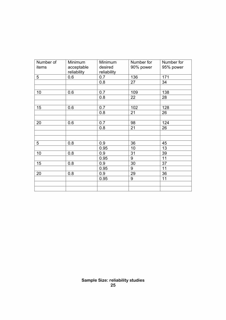
The reliability of a measurement scale is the degree to which all the items measure the same thing. In developing a new measurement scale, or showing that a measurement scale works on a new population, it is useful to measure its reliability. Reliability is measured using Cronbach's alpha coefficient, which is scaled between zero and one, with zero meaning that the items in the scale have nothing in common and one meaning that they are all perfectly correlated. In practice, it is wildly unlikely that anyone would develop a scale in which all the items were unrelated, so there is no point in testing whether your reliability is greater than zero. Instead, you have to specify a minimum value for the reliability coefficient. A value of 0.6 is usually taken as indicating that the scale has inadequate reliability. The second value you have to stipulate is the value at which the scale would be useful. Nunnally and Bernstein1 recommend a value of at least 0.7 for a scale under development, but where the scale will be used to make judgments about individuals (such as screening for mood disorders or selecting people for jobs) then a value of at least 0.9 is needed, and ideally 0.95. Step 1 Decide on the reliability at which the scale would be unacceptable. Recommendation: use 0.6 for scale development and 0.8 for scales that are used to make decisions about individuals. Step 2 Decide on the minimum reliability that would be needed for a worthwhile scale. Recommendation: set a minimum of 0.8 for scale development, and a value of 0.9 for scales that are to be used to make decisions about people. Step 3 Decide how many items are to be in the scale

1 Nunnally JC and Bernstein IH. Psychometric Theory, 3rd ed. New York, McGraw-Hill 1994

Sample Size: reliability studies 25

Number of items

Minimum acceptable reliability

Minimum desired reliability

Number for 90% power

Number for 95% power

5 0.6 0.7 136 171

0.8 27 34

10 0.6 0.7 109 138

0.8 22 28

15 0.6 0.7 102 128

0.8 21 26

20 0.6 0.7 98 124

0.8 21 26

5 0.8 0.9 36 45

0.95 10 13

10 0.8 0.9 31 39

0.95 9 11

15 0.8 0.9 30 37

0.95 9 11

20 0.8 0.9 29 36

0.95 9 11

Sample Size: when nothing is known in advance 26

Sample size for animal experiments in which not

enough is known to calculate statistical power

In animal experiments, the investigator may have no prior literature to turn to. The potential means and standard deviations of the outcomes are unknown, and there is no reasonable way of guessing them. In a case like this, sample size calculations cannot be applied.

The resource equation method

The resource equation method can be used for minimising the number of animals committed to an exploratory study. It is based on the law of diminishing returns: each additional animal committed to a study tells us less than the one to reach the threshold where adding further animals will be uninformative. It should only be used for pilot studies or proof-of-concept studies.

Applying the resource equation method

1. How many treatment groups will be involved? Call this T.

2. Will the experiment be run in blocks? If so, how many blocks will be used? Call this B

A block is a batch of animals that are tested at the same time. Each block may have a different response because of the particular conditions at the time they were tested. Incorporating this information into a statistical analysis will increase statistical power by removing variability between experimental conditions on different days.

3. Will the results be adjusted for any covariates? If so, how many? Call this C

Covariates are variables that are measured on a continuous scale, such as the weight of the animal or the initial size of the tumour. Results can be adjusted for such variables, which increases statistical power.

4. Combine these three figures:

(T–1) + (B+C–1) = D

Sample Size: when nothing is known in advance 27

5. Add at least 10 and at most 20

The sample size should be at least (D+10) and at most (D+20).

Example of the resource equation method

An investigator wishes to examine the effect of a new delivery vehicle for an anti-inflammatory drug. The experiment will involve four treatments: a control, a group receiving a saline injection, a group receiving the vehicle alone and a group receiving the vehicle plus drug. Because of laboratory limitations, only four animals can be done on one day. The experimenter doesn't plan on adjusting the results for factors like the weight of the animal. In this case, T (treatments) is 4 and C (covariates) is zero. So the sample size is at least 10 + (T–1) which is 10 + 3, which is 13. However, 13 animals will have to be done in at least 3 batches (assuming that the lab could manage a batch of five). This means that the experiment will probably have a minimum of 3 blocks, and more likely four. So, taking the blocks into consideration, the minimum sample size will be 10 + (T–1) + (B–1), which is 10 + 3 + 3, which is 16 animals. The experimenter might like to aim for the maximum number of animals, to reduce the possibility that the experiment will come to a false-negative conclusion. In this case, 20 + (T–1) suggests 23 animals, which will have to be done in 6 blocks of four. 20 + (T–1) + (B–1) is 28, which means running 7 blocks of four, which requires another adjustment: an extra animal is needed because the number of blocks is now 7. The final maximum sample size is 29. As you can see, when you are running an experiment in blocks, the sample size will depend on the number of blocks, which, in turn, may necessitate a small adjustment to the sample size.

Sample Size: Resources on the intenet 28

Resources for animal experiments

There are several excellent papers on reducing the numbers of animals needed in animal research. FRAME (http://www.frame.org.uk/index.htm) publishes and links to a number of papers. The following are recommended reading, and include information on sample size, http://embryo.ib.amwaw.edu.pl/invittox/er/ER/ER%2029.pdf http://www.frame.org.uk/atlafn/statsguidelines.pdf The Institute for Laboratory Animal Research has a whole issue of their journal devoted to the subject: http://dels.nas.edu/ilar_n/ilarjournal/43_4/ There is a collection of useful papers at http://embryo.ib.amwaw.edu.pl/invittox/er There are also good general guidelines on http://www.rgs.uci.edu/ora/rp/acup/policies/animalnumbers.htm


Computer and online resources

Standard statistical packages

Don't forget that many statistical packages will do sample size calculation. JMP does (read the help file before you fill in the dialog!). Stata also has a sample size routine, and there are many user-written routines to calculate sample sizes for various types of study. Use the command findit sample size to get a listing

of user-written commands that you can install. The free professional package R includes sample size calculation (but requires a lot of experience to use!) And no; SPSS will sell you a sample size package, but it isn't included with SPSS itself.

Sample size calculators and Online resources

You can look for sample size software to download at http://statpages.org/javasta2.html The Graph Pad website has a lot of helpful resources http://graphpad.com/welcome.htm They make an excellent sample-size calculator application called StatMate which gets high scores for a simple, intelligent interface and very useful explanations of the process. It has a tutorial that walks you through. http://graphpad.com/StatMate/statmate.htm There is a Windows sample size calculator at http://homepage.usask.ca/~jic956/work/MorePower.html and the very useful free package Epicalc 2000 includes sample size calculation as well as a host of useful ways of analysing tabulated data http://www.brixtonhealth.com/epicalc.html There is a free calculator for the Palm at http://www.bobwheeler.com/stat/SSize/ssize.html which includes a very extensive manual. The interface is a bit sparse but the manual makes it all clear.

Try the online sample size calculators at

http://home.clara.net/sisa/sampshlp.htm http://statpages.org/index.html#Power http://hedwig.mgh.harvard.edu/sample_size/size.html


Good help pages at http://www.cmh.edu/stats/size.asp and both help and online calculation at http://www.stat.uiowa.edu/~rlenth/Power/ There is a free Windows power calculation program at Vanderbilt Medical Center http://biostat.mc.vanderbilt.edu/twiki/bin/view/Main/PowerSampleSize Gerard van Belle's chapter on rules of thumb for sample size calculation can be downloaded from his website (http://www.vanbelle.org/) It's extracted from his book and is the only downloadable chapter. Finally, Ask Professor Mean is an excellent resource for all your statistical queries. The page relevant to sample size is at http://www.cmh.edu/stats/size.asp

sam ple size a rough guide -...

Documents