s o c r a t i c l e c t u r e s
TRANSCRIPT

S O C R A T I C L E C T U R E S
5TH INTERNATIONAL MINISYMPOSIUM, LJUBLJANA, 16. APRIL 2021
PEER REVIEWED PROCEEDINGS
EDITED BY: VERONIKA KRALJ-IGLIČ
FACULTY OF HEALTH SCIENCES, UNIVERSITY OF LJUBLJANA

I
Socratic lectures 5th International Minisymposium, Ljubljana, April 16., 2021 Peer Reviewed Proceedings Edited by Prof. Veronika Kralj-Iglič, Ph.D. Reviewers: Prof. Rok Vengust, M.D., Ph.D., Karin Schara, M.D., Ph. D. Published by: University of Ljubljana, Faculty of Health Sciences Design and photos: Anna Romolo, Matevž Tomaževič, Veronika Kralj-Iglič Image on the front page: Matevž Tomaževič Publication is available online in PDF format at: https://www.zf.uni-lj.si/images/stories/datoteke/Zalozba/Sokratska_5.pdf Ljubljana, 2021
This work is available under a Creative Commons Attribution 4.0 International
___________________
Kataložni zapis o publikaciji (CIP) pripravili v Narodni in univerzitetni knjižnici v Ljubljani
COBISS.SI-ID 69120259
ISBN 978-961-7112-05-4 (PDF)
___________________

II
The members of the Organizing Committee of Socratic Lectures: Kralj Iglič
Veronika, Vauhnik Renata, Stražar Klemen, Kristan Anže, Prelovšek Anita
Program
Socratic Symposium April 16, 2021, 16:00 – 20:00 (Ljubljana time)
Plenary lecture 16:00 – 16:45 Soeballe Kjeld, Aarhus University Hospital, Aarhus, Denmark: Surgical
treatment of acetabular dysplasia 16:45 –16:50 Weiss Silvius Leopold: Fantasia. Guitar: Masi Giovanni 16:50 - 17:00 Break
Parallel Sections Section 1: Emergent Problems in Orthopaedics and Traumatology
organized and moderated by Stražar Klemen and Kristan Anže, University Medical Centre
Ljubljana, Ljubljana, Slovenia
17:00-17:25 Spasovski Duško, Banjica Clinics, Belgrade, Serbia: Operative treatment of hip
dysplasia
17:25-17:50 Skala-Rosenbaum Jiri, University Medical Centre Prague, Czech Republik: Femur
malrotation after trochanteric fracture: incedence and concequences
17:50-18:15 Stražar Klemen, University Medical Centre Ljubljana, Ljubljana, Slovenia: Limits of
hip arthroscopy
18:15-18.20 Break
18:20-18:45 Atul Kamath, Cleveland Clinic, Cleveland, U.S.A., Role of hip preservation in 2021
18:45-18.55 Kristan Anže, University Medical Centre Ljubljana, Ljubljana, Slovenia, Influence of
implant placement and of reduction of trochanteric fractures type A2 on mobility
of the patient after healing of the fracture and on probability of mechanical
failures
18:55-19:05 Šarler Taras, University Medical Centre Ljubljana, Ljubljana, Slovenia, Anatomic
and kinematic planning of arthroscopic femoroacetabular osteoplasty
19:05-19:15 Jug Marko, University Medical Centre Ljubljana, Ljubljana, Slovenia, Spinal cord
injury and decompression- a question of time and pressure
19:15-19:25 Ambrožič Miha, Kovačič Ladislav: University Medical Centre Ljubljana, Ljubljana,
Slovenia, Platelet-rich plasma injection following arthroscopic rotator cuff repair -
Is there any benefit?
19:25-19:35 Tomaževič Matevž, University Medical Centre Ljubljana, Ljubljana, Slovenia, The
effect of stress distribution in artificial hip joint on the dislocation of the hip
endoprosthesis
19:35-19:45 Zore Anderj Lenart, University Medical Centre Ljubljana, Ljubljana, Slovenia,
Computer assistance in periacetabular osteotomy

III
Section 2: Emergent Problems in Physiotherapy organized and moderated by Vauhnik Renata and Rugelj Darja, University of Ljubljana, Faculty of Health Sciences 17:00-17:30 Daniel Munoz Garcia, University La Salle, Madrid, Spain, Prior cortical activity
differences during an action observation plus motor imagery task related to motor performance of a coordinated multi-lmb complex task.
17:30-18:00 Alon Wolf, Technion, Israel Institute of Technology, Faculty of Mechanical Engineering, Haifa, Israel, Biomechanics: When science and engineering meet sport
18:00-18:30 Carmen Belen Martinez Cepa, Juan Carlos Zuil Escobar, Rocio Palomo, University CEU San Pablo, Madrid, Spain, Action observation therapy combined with mirror therapy in children with unilateral cerebral palsy: randomized controlled trial protocol and feasibility study
18:30 - 18:45 Darja Rugelj, University of Ljubljana, Faculty of Health Sciences, Ljubljana, Slovenia: Postural sway on inclined surfaces
18:45-19:00 Renata Vauhnik, University of Ljubljana, Faculty of Health Sciences, Ljubljana, Slovenia: Can we decrease knee anterior laxity?
19:00-19:15 Marko Vidovič, University of Ljubljana, Faculty of Health Sciences, Ljubljana, Slovenia: Increasing hand dexterity through the use of various somatosensory stimuli such as vibration, electrical stimulation, and textured materials
19:15-19:30 Helena Žunko, University of Ljubljana, Faculty of Health Sciences, Ljubljana, Slovenia: Ankle dorisflexion range of motion measurement tools
19:30-19:45 Maja Petrič, University of Ljubljana, Faculty of Health Sciences, Ljubljana, Slovenia: The effect of yoga and stabilization exercises on trunk muscle endurance and flexibility in healthy adults
Section 3: Free topics organized and moderated by Prelovšek Anita 17:00-17:45 Muršič Rajko, University of Ljubljana, Faculty of Philosophy, Ljubljana, Slovenia:
Creativity and music - essential elements in human development 17:45-18:45 Paliska Nelfi, Music School Koper, Koper, Slovenia, Mozart's travels to Italy 18:45-19:15 Gala Kušej Nina, Protocol of Republic of Slovenia, Music and protocol 19:15-19:30 Pečan Irenej, Jeran Marko, University of Ljubljana, Faculty of Health Sciences,
Ljubljana, Slovenia: Step into the Future by Bauman Moscow State Technical University & Russian Youth Engineering Society.
19:30 - 19:45 Ipavec Marija, Government of Republic of Slovenia, 42 years of experience with above-knee prosthesis.
20:00 Closing Ceremony with Cultural program. Chopin Frederic: Variations on the theme by Giaccomo Rossini; flute: Prelovšek Anita

IV
Editorial
In the academic year 2020/2021 the Socratic Lectures were organized twice: in December, with
co-production of the Ves4us consortium, and in April. This was a reflection of the decision of the
Medical Faculty to reorganize the performance of the optional courses into the “package” form, to
be completed in November or in June. The course “Biomechanics of joints” was completed in the
first semester and as the Socratic Lectures have always been the final event of the course, the
symposium was organized in December 2020. The original timing of the course Special
biomechanics for students of the 1st year of Orthotics and Prosthetics at the Faculty of Health
Sciences remained the same (February –April) and ended with Socratic Lectures as the final event
in April.
The online form of the symposium enabled participation of world top professionals and scientists.
Following the inspiring plenary lecture given by prof. Kjeld Soeballe from Aarhus University
Hospital, Aarhus, Denmark, the symposium featured tree sections: Emergent problems in
Orthopaedics and Traumatology, Emergent problems in Physiotherapy and Free topics. The
members of the organizing committee were prof. Veronika Kralj-Iglič, prof. Klemen Stražar, prof.
Anže Kristan, prof. Renata Vauhnik, prof. Darja Rugelj and dr. Anita Prelovšek. Cultural program
was performed by dr. Anita Prelovšek on the flute and by Giovanni Masi on the guitar.
Anita Prelovšek, PhD, studied flute in Ljubljana, Slovenia and in Trieste, Italy and finished
postgraduate studies in France. She is a free-lance artist and performs worldwide. Also she
completed postgraduate study of Musicology at the University of Ljubljana, Faculty of Philosophy.
Her choice in Socratic Lectures was Variations on a Theme of Rossini in E major for flute by Frederic
Chopin.
Giovanni Masi (2002) studied guitar at the musical high school P.E. Imbriani, Avellino, Italy under
the guidance of Mº Gianluca Allocca and currently attends the specialized guitar course at the D.
Cimarosa Conservatory, Avellino, under the guidance of Mº Lucio Matarazzo. He is performing
publicly since he was 14 years old and has won over 20 national and international competitions. At
Socratic Lectures he performed Fantasia by Silvius Leopold Weiss (1687-1750).
An addition to the present issue were photographs taken by Matevž Tomaževič in Namibia shortly
after the symposium. He participated at the symposium with a contribution which was a subject of
his PhD that took place a day before the symposium.
The April Socratic Lectures was a meaningful event that will remain in the memories of the
participants (the joint section was attended by approximately 120 participants), in particular the
students.
Veronika Kralj-Iglič, Anna Romolo

V
Contents
1. Kristan Anže: How can we influence the mobility of the patients and probability
of mechanical failures in trochanteric fractures type A2? ……………………………………………2
2. Tomaževič Matevž, Cimerman Matej , Kralj Iglič Veronika: The effect of stress
distribution in artificial hip joint on the dislocation of the hip endoprosthesis……………..8
3. Stražar Klemen : Limits of hip arthroscopy………………………………………………………………….21
4. Jug Marko:Spinal cord injury and decompression- a question of time and pressure…..27
5. Ambrožič Miha, Kovačič Ladislav : Platelet-rich plasma injection following
arthroscopic rotator cuff repair: Is there any benefit?...................................................33
6. Šarler Taras, Stražar Klemen: Anatomic and Kinematic Planning of Arthroscopic
Femoroacetabular Osteoplasty ………………………………………………………………………………….50
7. Zore Lenart Andrej, Stražar Klemen: Computer assistance in periacetabular
Osteotomy.………………………………………………………………….................................................60 8. Vidovič Marko, Rugelj Darja : Increasing hand dexterity through the use of
various somatosensory stimuli: a pilot study………………………………………………………………66 9. Rugelj Darja, Bedek Jure, Benko Žiga, Drobnič Matej, Vauhnik Renata: The effect
of knee extensor and flexor strengthening, coupled with passive anterior tibial
translation, on knee anterior laxity in the ACL injured knee. A case report…………..…….78
10. Rugelj Darja, Pilih Iztok , Vauhnik Renata : Effect of repeated passive anterior
loading on knee anterior laxity in injured knee: case report……………………………………….86
11. Leban Pia, Baucon Kralj Mojca, Griessler Bulc Tjaša, Prosenc Franja: Extraction
of polyethylene terephthalate (PET) microplastics from alluvial soil: comparison
of density separation and oil-based extraction…………………………………………………………..93
12. Jeran Marko, Božič Darja, Novak Urban, Hočevar Matej, Romolo Anna, Iglič Aleš,
Kralj-Iglič Veronika : European spruce (Picea abies) as a possible sustainable source
of cellular vesicles and biologically active compounds …………………………………………….104
13. Koren Jerneja, Scott Derek, Jeran MarKo : Renin-angiotensin system inhibitors
and their implications for COVID-19 treatment………………………………………………………..115
14. Pečan Luka Irenej, Štukelj Roman, Torkar Godič Karmen, Jeran Marko : Study
of the cannabinoid profile and microbiological activity of industrial hemp
(Cannabis Sativa subsp. Sativa L.)……………………………………………………………………………..125
15. Jan Zala: In vitro cell experiments as important approach in cellular vesicles
research……………………………………………………………………………………………………………………140
16. Kušej Gala Nina: Music and protocol………………………………………………………………………. 149
17. Prelovšek Anita : The role of painting in the life and works of Fyodor Mikhailovich
Dostoevsky ……………………………………………………………………………………………………………..156
18. Romolo Anna, Kralj-Iglič Veronika : The wanishing memory of the bourgeois
world in Rožna dolina and Mirje districts in Ljubljana, Slovenia……..…………………………177
19. Rugelj Darja : Postural sway on inclined surfaces……………………………………………………….188

1

2
___________________
How can we influence the mobility of the patients and probability of
mechanical failures in trochanteric fractures type A2?
Kristan Anže*
Department of Traumatology, University Medical Centre Ljubljana, Ljubljana, Slovenia
Abstract
In the first part of this paper, we are discussing the influence of reduction and implant
placement on position of the healed trochanteric fracture AO/OTA A2 and how it influences
the walking ability after healing. In the second part we are analysing factors which can be
influenced during the surgery and can lead to mechanical failure and reoperation in these
fractures.
___________________
3
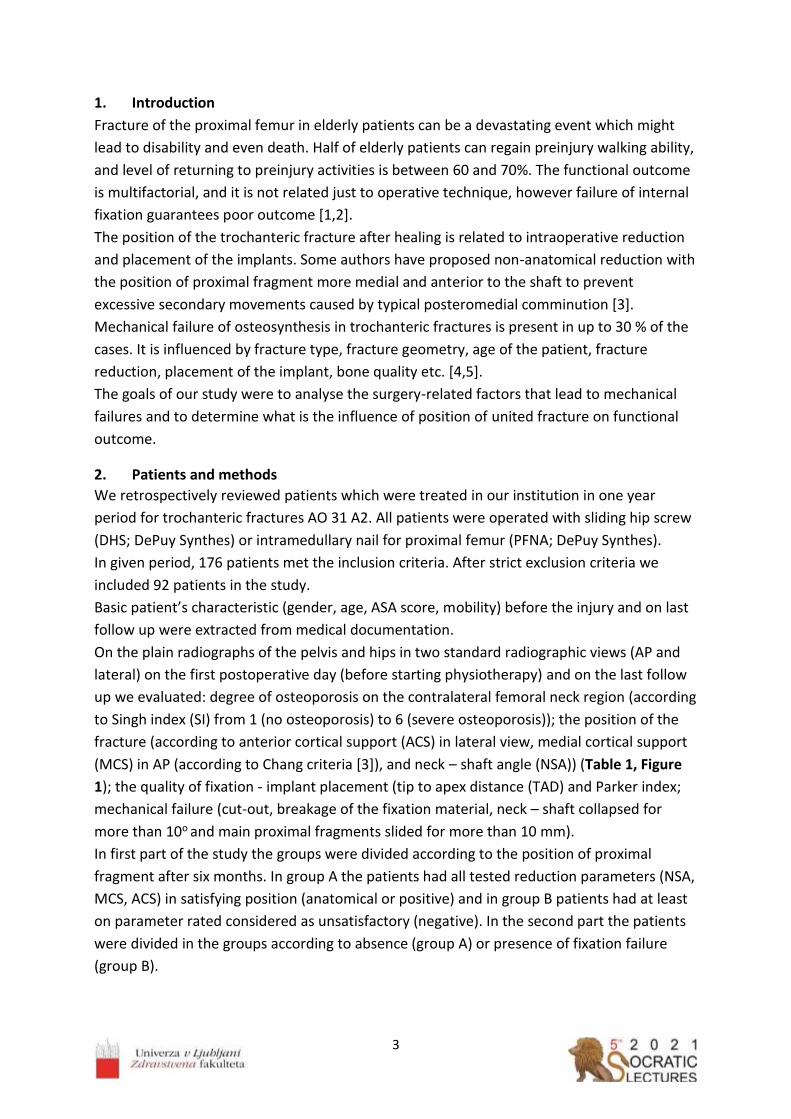
1. Introduction
Fracture of the proximal femur in elderly patients can be a devastating event which might
lead to disability and even death. Half of elderly patients can regain preinjury walking ability,
and level of returning to preinjury activities is between 60 and 70%. The functional outcome
is multifactorial, and it is not related just to operative technique, however failure of internal
fixation guarantees poor outcome [1,2].
The position of the trochanteric fracture after healing is related to intraoperative reduction
and placement of the implants. Some authors have proposed non-anatomical reduction with
the position of proximal fragment more medial and anterior to the shaft to prevent
excessive secondary movements caused by typical posteromedial comminution [3].
Mechanical failure of osteosynthesis in trochanteric fractures is present in up to 30 % of the
cases. It is influenced by fracture type, fracture geometry, age of the patient, fracture
reduction, placement of the implant, bone quality etc. [4,5].
The goals of our study were to analyse the surgery-related factors that lead to mechanical
failures and to determine what is the influence of position of united fracture on functional
outcome.
2. Patients and methods
We retrospectively reviewed patients which were treated in our institution in one year
period for trochanteric fractures AO 31 A2. All patients were operated with sliding hip screw
(DHS; DePuy Synthes) or intramedullary nail for proximal femur (PFNA; DePuy Synthes).
In given period, 176 patients met the inclusion criteria. After strict exclusion criteria we
included 92 patients in the study.
Basic patient’s characteristic (gender, age, ASA score, mobility) before the injury and on last
follow up were extracted from medical documentation.
On the plain radiographs of the pelvis and hips in two standard radiographic views (AP and
lateral) on the first postoperative day (before starting physiotherapy) and on the last follow
up we evaluated: degree of osteoporosis on the contralateral femoral neck region (according
to Singh index (SI) from 1 (no osteoporosis) to 6 (severe osteoporosis)); the position of the
fracture (according to anterior cortical support (ACS) in lateral view, medial cortical support
(MCS) in AP (according to Chang criteria [3]), and neck – shaft angle (NSA)) (Table 1, Figure
1); the quality of fixation - implant placement (tip to apex distance (TAD) and Parker index;
mechanical failure (cut-out, breakage of the fixation material, neck – shaft collapsed for
more than 10o and main proximal fragments slided for more than 10 mm).
In first part of the study the groups were divided according to the position of proximal
fragment after six months. In group A the patients had all tested reduction parameters (NSA,
MCS, ACS) in satisfying position (anatomical or positive) and in group B patients had at least
on parameter rated considered as unsatisfactory (negative). In the second part the patients
were divided in the groups according to absence (group A) or presence of fixation failure
(group B).

4
Table 1. Reduction criteria according to Chang.
reduction anatomical positive negative
parameter
NSA 125o – 137o > 137o < 125o
MCS anatomical medial to the shaft lateral to the shaft
ACS anatomical anterior to the shaft posterior to the shaft
NSA: neck-shaft angle, MCS: medial cortical support, ACS: anterior cortical support.
Figure 1. Reduction criteria according to Chang. If proximal fragment is anteriorly to the shaft, ACS it is positive
(+ACS), if it is posteriorly to the shaft, ACS is negative (-ACS). If proximal fragment is medial to the shaft, MCS is positive
(+MCS) if it is lateral to the shaft, MCS is negative (-MCS).
3. Results
In first part we divided our patients in two groups according to position of united fractures
(Group A – good position; group B – unsatisfying). We had equal number of patients in both
groups (46). They did not differ in basic patients’ characteristics, degree of osteoporosis,
type of implant used or placement.
The only significant difference was in reduction parameters during the surgery, which got
worse during the healing (Table 2).

5
Table 2. Comparison of groups A and B in reduction parameters after the surgery and six months later (in
statistical probability of the t-test pertaining to the difference between the groups)
reduction A vs. B (op) A vs. B (6m) A (op) vs. A (6m) B (op) vs. B (6m)
NSA 0.074 0.003 0.290 0.719
MCS 0.057 < 0.001 0.014 0.002
ACS 0.001 < 0.001 0.076 0.435
A: group A, B: group B, op: immediately after the surgery, 6m: six months after the surgery, NSA: neck-shaft
angle, MCS: medial cortical support, ACS: anterior cortical support.
These differences influence the mobility level after healing. In both groups the mobility was
worse after the healing of the fracture comparing to the preinjury level. But in group B the
difference was bigger. (Table 3) [6]. We found statistically significant difference in mobility
between Group A and Group B determined 6 months after the surgery (p = 0.029).
Table 3. Comparing mobility level before injury and six months after the surgery for groups A and B.
mobility Group A n (%)
Group A 6m n (%)
p Group B n (%)
Group B 6m n (%)
p
no assistance 31 (67.4%) 16 (34.8%) 25 (54.3%) 5 (10.9%)
assistance 15 (32.6%) 28 (60.8%) 0.006 21 (45.7%) 37 (80.4) <0,001
wheelchair 0 (0%) 2 (4.4%) 0 (0%) 4 (8.7%)
n: number of patients, p: p-value - statistical probability, op: postoperatively, 6m: six months after the surgery
In the second part of the study, we compared patients with mechanical failure (group B) to
those with uneventful healing (group A). In group B there were 30 % of all operated patients.
Less frequent was most catastrophic event of cut-out which happened in 4.2% of our
patients, followed by neck – shaft collapse (for more than 10o) in 8.3 %. The most frequent
was excessive sliding of main proximal fragments (for more than 10 mm) - in 16.7%. There
were no cases of breakage of osteo-synthetic material in our series. The only difference
between groups at the surgery was reduction in MCS. At follow up, the differences were
significant in all parameters except NSA and TAD (Table 4) [7].
Table 4. Comparison of groups A and B in reduction parameters after the surgery and six months later.
Probability pertaining to the difference between the groups, calculated by the t-test is given.
Parameter A vs. B (OP) A vs. B (FU)
NSA 0.860 0.892
MCS 0.006* < 0.001*
ACS 0.246 0.001*
TAD 0.546 0.092
PIAP 0.213 0.029*
PIL 0.828 0.015*
A: group A, B: group B, OP: immediately after the surgery, FU: last follow up, NSA: neck-shaft angle, MCS: medial cortical support, ACS: anterior cortical support, TAD: tip to apex distance, PIAP: Parker index in anteroposterior projection, PIL: Parker index in lateral projection, *: statistically significant.

6
4. Conclusions In our study we clearly showed the influence of unsatisfactory position of the proximal
fragment on walking ability of patients with trochanteric fracture type A2 after half a year.
With retrograde analysis from the known outcome, we were able to show decisive influence
of anterior cortical support on final position of proximal fragment. The parameters which
were controlled in anteroposterior projections were less important, however more attention
during surgery should be put on anterior cortical support in the future.
Regarding mechanical failure we can conclude that reduction in AP view is the most
important prognostic factor for mechanical failure of A2 trochanteric fractures. However the
effects of NSA, ACS and the position of the implant should be considered in the future.
Knowing that the proximal fragment is a three-dimensional structure, it is not possible to
strictly divide ACS, MCS and NSA when judging the quality of reduction. In future studies,
more attention must be devoted to rotational malalignment of the proximal fragment itself.
Its relation to the shaft of the femur would give some additional information on position of
the fracture (NSA, MCS and ACS) and on its influence on mechanical failure and functional
outcome.
References
1. Shah MR, Aharonoff GB, Wolinsky P, Zuckerman JD, Koval KJ. Outcome afterhip fracture
in individuals ninety years of age and older. J Orthop Trauma.2001; 15(1):34–39.
doi: 10.1097/00005131-200101000-00007
2. Koval KJ, Skovron ML, Aharonoff GB, Zuckerman JD. Predictors of functional recovery
after hip fracture in the elderly. Clin Orthop Relat Res. 1998; 348:22–28.
3. Chang SM, Zhang YQ, Du SC, Ma Z, Hu SJ, Yao XZ, et al. Anteromedial cortical support
reduction in unstable pertrochanteric fractures: a comparison of intra-operative
fluoroscopy and post-operative three-dimensional computerized tomography
reconstruction. Int Orthop. 2018; 42(1):183-189. doi: 10.1007/s00264-017-3623-y
4. Hsueh KK, Fang CK, Chen CM, Su YP, Wu HF, Chiu FY. Risk factors in cutout of sliding hip
screw in intertrochanteric fractures: an evaluation of 937 patients. Int Orthop. 2010;
34(8):1273-1276. doi: 10.1007/s00264-009-0866-2
5. Ye KF, Xing Y, Sun C, Cui ZY, Zhou F, Ji HQ, Guo Y, Lyu Y, Yang ZW, Hou GJ, Tian Y, Zhang
ZS. Loss of the posteromedial support: a risk factor for implant failure after fixation of
AO 31-A2 intertrochanteric fractures. Chin Med J (Engl). 2020; 5;133(1):41-48.
doi: 10.1097/CM9.0000000000000587
6. Kristan A, Benulič Č, Jaklič M. Influence of reduction and implant placement on
mechanical failure in A2 type of trochanteric fractures. AOTT. 2021 in revision.
7. Kristan A, Benulič Č, Jaklič M. Reduction of trochanteric fractures in lateral view is
significant predictor for radiological and functional result after six months. Injury. 2021;
S0020-1383(21)00141-8. doi: 10.1016/j.injury.2021.02.038

7

8
_________________
The effect of stress distribution in artificial hip joint on the dislocation of the
hip endoprosthesis
Tomaževič Matevž1,*, Cimerman Matej1, Kralj Iglič Veronika2. 1University Medical Centre Ljubljana, Department of Traumatology, Ljubljana, Slovenia 2University of Ljubljana, Faculty of Health Sciences, Laboratory of Clinical Biophysics,
Ljubljana, Slovenia
Abstract
Dislocation after hip arthroplasty is still a major concern. Recent study of the volumetric
wear of the cup has suggested that stresses studied in a one-legged stance model could
predispose arthroplasty dislocation. The aim of this work was to study whether
biomechanical parameters of contact stress distribution in total hip arthroplasty during a
neutral hip position can predict a higher possibility of the arthroplasty dislocating.
Biomechanical parameters were determined using 3-dimensional mathematical models of
the one-legged stance within the HIPSTRESS method. Geometrical parameters were
measured from standard anteroposterior X-ray images of the pelvis and proximal femora.
Fifty-five patients subjected to total hip arthroplasty that later suffered dislocation of the
head and, for comparison, 95 total hip arthroplasties that were functional at least 10 years
after the implantation, were included in the study. Arthroplasties that suffered dislocation
had on average a 6% higher resultant hip force than the control group (p=0.004), 11% higher
peak stress on the load-bearing area (p=0.001) and a 50% more laterally positioned stress
pole (p=0.026), all parameters being less favorable in the group of unstable arthroplasties.
There was no statistically significant difference in the hip gradient index or in the functional
angle of the weight bearing. Our study showed that arthroplasties that show a tendency to
push the head out of the cup in the representative body position - the one-legged stance -
are prone to dislocation. An unfavorable resultant hip force, peak stress on the load bearing
and laterally positioned stress pole are predictors of arthroplasty dislocation.
_________________

9
1. Introduction
Based on patient reported outcome measures, hip arthroplasty is the most successful
elective surgical procedure [1]. Today more than 95% of arthroplasties survive more than 10
years [2,3]. Some total hip arthroplasties (THAs) nevertheless fail and revision surgery is
needed. Hip dislocation after THA is the second most common cause of revision surgery [2].
The reported rate of revision due to dislocation after primary THA is 2-4 % in the first six
months [4] and increases to 6% after 20 years [5]. After revision surgery, the dislocation rate
levels at 5.4% in the first year after the operation [6]. Dislocation studies of THA have been
performed based on component positioning, with an emphasis on cup orientation [7-10], the
effect of artificial head size [5,11,12] and impingement as causes of a prosthesis head
dislocation [13-15]. More than 50 % of dislocations occur when the cup is in the so-called
safe zone position [10]. A larger femoral head diameter increases the range of motion before
the prosthesis neck impinges on the acetabulum liner, which causes the prosthesis to
dislocate [5,11,16]. Despite the careful positioning of THA components, dislocations still
occur. The question arises as to whether THA changes the geometry of the hip in such a way
to affect the biomechanical parameters in the joint, forcing the hip to dislocate at the edge
of the motion range.
The HIPSTRESS method was developed to calculate biomechanical parameters in the hip
considering pelvis and femur anatomy [17,18].
The HIPSTRESS method demonstrates that linear wear occurs in the direction of the stress
pole [19,20] and that it is proportional to the peak stress on the weight bearing area[19].
Because of this effect, the volumetric wear on the cup is less for a larger abduction angle of
the cup [21], since the head partly migrates out of the socket [21]. On the other hand, it has
been shown that this could be unfavorable in terms of dislocation [21].
The aim of this work was that check whether biomechanical parameters (higher peak stress,
more lateral position of stress pole and less negative stress gradient index) are predictors for
dislocation of a THA. To test this hypothesis, we compared the biomechanical parameters of
a THA population that had suffered dislocation and a THA population that did not dislocate
at least 10 years post-operatively.
2. Methods
The study was designed as a retrospective individual case control study, level of evidence 3B.
It was approved by Slovene National Medical Ethics Committee letter No.: 110/04/15.
Anteroposterior (AP) X-ray images of the hip and pelvic skeleton of patients that had
undergone THA were used to measure geometrical parameters relevant for a determination
of biomechanical parameters within the HIPSTRESS method. X-ray images of patients that
had suffered dislocation of hip arthroplasties were included in the study group. Patients
were chosen from the emergency department database based on a diagnosis of hip
dislocation, ICD S73.0. Patients admitted to the Emergency Department, University Clinical
Center Ljubljana from November 2012 until September 2015 were included. Images were
downloaded from the Impax server and coded. Eighty-one patients with a diagnosis of

10
dislocation of the hip joint were gathered. Exclusion criteria were patients that had suffered
hip dislocation due to high energy trauma (17 patients), patients with whom dislocation had
occurred due to material breakage of the hip prosthesis (2 patients), patients where the
contours of the femur or pelvis were not clearly visible on the X-ray image (1 patient) and
patients with partial endoprosthesis (6 patients). X-ray images taken immediately after
reduction of the dislocation were used for analysis. After excluding the patients with the
exclusion criteria, 55 patients remained in the study group. Twenty-five (41%) of them had
already undergone hip arthroplasty on the contralateral hip.
Standard X-ray images of the hip and pelvis taken at the Emergency Department, University
Medical Center Ljubljana were assumed to have an average magnification of 115% and the
size of the prosthesis head was estimated by rounding to 28mm, 32mm or 36 mm using
software developed for preoperative planning at the Department of Traumatology,
University Medical Center Ljubljana. Twenty-six (47%) hips in the study group with THA had a
femoral head diameter of 28 mm, 12 (22%) had a femoral head diameter of 32 mm and 17
(31%) had a femoral head diameter of 36 mm. On average, the radius of the prosthesis head
was 15.67 mm ± 1.75 mm.
To define the control group, we examined X-ray images of 311 patients who had undergone
total hip arthroplasty (THA) at the Orthopedic Hospital Valdoltra, Slovenia. The first available
X-ray images or THA with whole pelvis (in terms of date) were taken from the Impax server
at the hospital. Inclusion criteria were an X-ray image of the pelvis and proximal femora after
implantation, no event of hip dislocation or septic or aseptic loosening and regular follow-up
for at least 10 years. Patients who had undergone any revision procedure during that time
were also excluded. Ninety-four hips (54 (63%) right and 35 (37%) left) of 77 patients that
met the inclusion criteria (45 female and 32 male) were included in the analysis. Sixty-nine of
them also had a prosthesis on the contralateral side. The average age of the patients
included at the time of implantation was 59.6 years. There were 79 (84%) THA with a
femoral head diameter of 28mm, 2 (2%) of them had a femoral head diameter of 32 mm and
13 (14%) had a femoral head diameter of 36mm.
For biomechanical evaluation, three-dimensional mathematical models of an adult human
hip within the HIPSTRESS method were used [18,22]. The models are described in detail
elsewhere (see for example ref. [22]) so only a brief description will be given here. The
method consists of two mathematical models: one for determination of the resultant hip
force in the representative body position for everyday activities [23], i.e., the one-legged
stance (24), and the other for determination of contact hip stress distribution [17]. The
model for resultant hip force is based on force and torque equilibrium equations [18,24].
The model describes a system composed of two segments: the loaded leg and the rest of the
body. It includes 9 effective muscle forces, the weight of the segments and the intersegment
force (the resultant hip force). The reference muscle attachment points are obtained from
measurements performed on a cadaver and then re-scaled for the individual hip considered.
Since the X-ray image is two-dimensional, data in the third dimension are taken to be equal
to the reference values. The model for force uses as input the geometrical parameters of

11
pelvis and proximal femur: pelvic width (C) and height (H), inter-hip distance (l) and the
position of the muscle attachment point on the greater trochanter (x,z) (Figure 1). Stress
integrated over the load-bearing area yields the resultant hip force R = ʃ p dA, where p is
stress and dA is the area element. The calculations and procedures have been explained
previously [19,22,25,26].
HIPSTRESS models use hip and pelvis geometric parameters as input data: inter-hip distance
(l), height of the pelvis (H), horizontal distance from the prosthesis head center to the lateral
edge of the pelvis (C), position of the greater trochanter relative to the prosthesis head
center in the coordinate system of the femur (distances z and x) and abduction angle. The
geometrical parameters were determined using CorelDRAW Graphics Suite X7, 2015,
Ottawa, Canada, by two blinded measurers. HIPSTRESS software (26) was used for
calculation of the biomechanical parameters. (Figure 1). Previous studies [28-32] have
indicated that the peak stress on the load-bearing area pmax is a useful biomechanical
parameter. If the stress pole is located inside the load bearing area, pmax is equal to the value
of the stress at the pole. If the stress pole lies outside the load-bearing area, contact stress is
highest at the point of the load-bearing area that is closest to the pole,
pmax = p0 cos(/2 – ϑabd - Θpole) , (1)
where p0 is the value of stress at its pole, abd is the abduction angle of the prosthesis cup
and pole is the angle of the stress pole (Figure 1). Another indicator of the stress distribution
is the gradient of stress, represented by its value at the lateral rim of the cup Gp (Eq. (2))
[21,33]
Gp = - p0 cos( - ϑabd - Θpole)/r , (2)
where r is the radius of the articular surface. If the pole of stress distribution lies outside the
load-bearing area (i.e., if Θpole ˃ /2 – ϑabd), then Gp is positive, stress attains its highest value
at the lateral rim and falls off rapidly in the medial direction, while the corresponding weight
bearing area is small [34]. Such a distribution represents dysplastic hips [34]. If, however, the
pole of stress distribution lies inside the load–bearing area (if Θpole ˂ /2 – ϑabd), then stress
reaches its peak within the weight bearing area, which is consequently larger and Gp is
negative [34]. The functional angle of load bearing ϑf is defined as
ϑf = ( - ϑabd - Θpole) . (3)
In relation to dislocation, high resultant hip force and high peak stress are unfavorable.
However, a high gradient index and more laterally positioned pole are expected to represent
an even greater risk of dislocation, since the head is pushed more laterally each time the leg
is loaded.

12
Figure 1. Geometric and biomechanical parameters within the HIPSTRESS models that are used for calculation of
stress distribution in a right artificial hip. R resultant hip force; pmax peak stress on the load bearing area; pole
angle of the stress pole; abd abduction angle; R angle of the resultant hip force; C horizontal distance between the center of the prosthesis head and the most lateral point on the iliac crest; H vertical distance between the center of the prosthesis head and the highest point on the iliac crest; x vertical distance between the center of the prosthesis head and the point on the greater trochanter in the direction of the femur; z distance between the center of the prosthesis head and the point on the greater trochanter perpendicular to the femur axis; l distance between the centers of the femoral heads [27].
The peak stress pmax is proportional to r-2, while the hip stress gradient index Gp is
proportional to r-3 [17,34]. Since different sizes of prosthesis heads were involved, the effect
of the femoral head size on biomechanical parameters was eliminated by multiplying pmax by
r2 and Gp by r3. The resultant hip force, peak stress and stress gradient index are also
proportional to body weight Wb. Since the body weight was unknown, its effect was
eliminated by normalizing the respective parameters by Wb. The normalized biomechanical
parameters R/WB, pmaxr2/Wb, Gpr3/Wb, ϑf and Θpole express the geometry of the pelvis and
13
the proximal femur and the geometry and position of the arthroplasty’s elements (but not
the size of the artificial head).
Statistical analysis of the biomechanical parameters between the two groups was done using
the Student T - test. If the p value was ≤ 0.05, the difference between these two groups was
significant. The statistical power (1-β) of the result was taken as sufficient when the power
was ˃80%. Statistical analysis was done using Microsoft Excel 2010 (14.0.7188.5000,
Microsoft Corporation, Santa Rosa, California, USA). The power of the statistics was
calculated using a statistics power calculator on the internet:
http://clincalc.com/Stats/Power.aspx
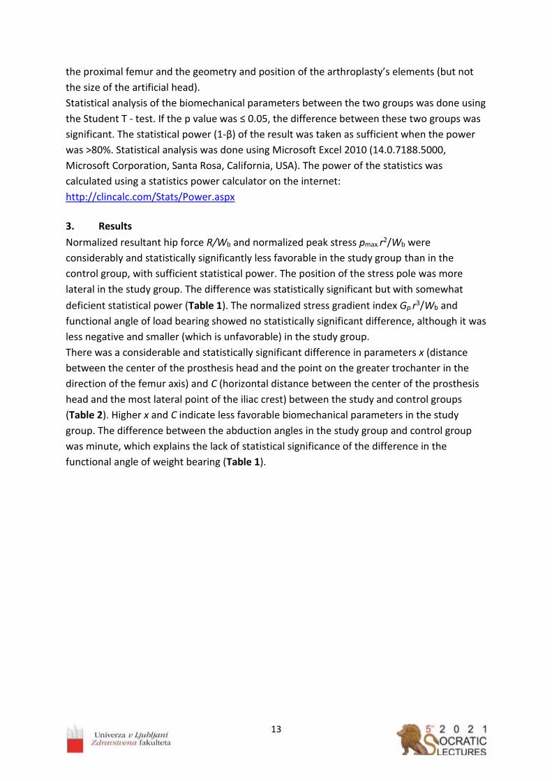
3. Results
Normalized resultant hip force R/Wb and normalized peak stress pmaxr2/Wb were
considerably and statistically significantly less favorable in the study group than in the
control group, with sufficient statistical power. The position of the stress pole was more
lateral in the study group. The difference was statistically significant but with somewhat
deficient statistical power (Table 1). The normalized stress gradient index Gpr3/Wb and
functional angle of load bearing showed no statistically significant difference, although it was
less negative and smaller (which is unfavorable) in the study group.
There was a considerable and statistically significant difference in parameters x (distance
between the center of the prosthesis head and the point on the greater trochanter in the
direction of the femur axis) and C (horizontal distance between the center of the prosthesis
head and the most lateral point of the iliac crest) between the study and control groups
(Table 2). Higher x and C indicate less favorable biomechanical parameters in the study
group. The difference between the abduction angles in the study group and control group
was minute, which explains the lack of statistical significance of the difference in the
functional angle of weight bearing (Table 1).

14
Table 1. Comparison of biomechanical parameters of the hips with THA in the study and control group.
R/Wb, resultant hip force normalized by body weight; pmax*r2/Wb; effect of pelvis geometry on peak stress on the load bearing area normalized by body weight; Gp*r3/Wb; effect of pelvic geometry on the peak hip gradient
index; f (°), functional angle of the load bearing; pole (°), position of the stress pole. (*) An asterisk denotes a value with higher risk for dislocation.
Table 2. Comparison of geometrical parameters of the hips with THA in the study group and control group
H (mm), vertical distance between the center of the prosthesis head and the highest point on the iliac crest; z (mm), distance between the center of the prosthesis head and the point on the greater trochanter perpendicular to the femur axis; x (mm), vertical distance between the center of the prosthesis head and the point on the greater trochanter in the direction of the femur; C (mm), horizontal distance between the center of the prosthesis head and the most lateral point on the iliac crest; l (mm), horizontal distance between the
right and left center of the femoral head; abd (°), abduction angle. (*) An asterisk denotes a value with a higher risk of dislocation.
Average ± SD Study group (55 THA)
Control group (94 THA)
Difference (%) p Power (1-β)
R/Wb mean 2.71 (SD 0.36)*
mean 2.54 (SD 0.32)
6.3 0.004 89.9%
pmax*r2/Wb mean 152.11 (SD 37.04)*
mean 135.32 (SD 21.42)
11.0 0.001 92.7%
Gp*r3/Wb mean -828287.70 (SD 413381.01)*
mean -871926.04 (SD 220240.41)
-5.27 0.400 10.9%
f (°) mean 129.13 (SD 17.57)
mean 132.90 (SD 13.60)
-2.9 0.146 39.5%
pole (°) mean 5.77 (SD 9.71)*
mean 2.86 (SD6.08)
50.0 0.026 62.9%
Average ± SD Study group (55 THA)
Control group (94 THA)
Difference (%) P Power (1-β)
H (mm) mean 136.80 (SD 13.53)
mean 133.78 (SD11.18)
2.2 0.144 40.6%
z (mm) mean 56.73 (SD 8.71)
mean 59.18 (SD 6.73)
-4.3 0.057 56.3%
x (mm) mean 14.77 (SD 8.69)*
mean 7.81 (SD 5.34)
47.1 0.000 100%
C (mm) mean 59.58 (SD 8.87)*
mean 55.52 (SD 9.22)
6.8 0.010 84.8%
l (mm) mean 179.61 (SD 11.15)
mean 177.13 (SD 10.26)
1.38 0.169 10.9%
abd (°) mean 45.10 (SD9.12)
mean 44.24 (SD 7.97)
1.9 0.547 14.5%

15
4. Discussion
Our study proved that contact stress distribution on the prosthesis head is a predictor of
arthroplasty dislocation.
It is shown above (Table 1) that THA that had suffered dislocation had a less favorable
distribution of contact stress (given by its peak value and the position of the pole), which
pushed the artificial head more laterally than in the case of prostheses that were functional
at least 10 years post-operatively. A previous study had shown that the head migrates in the
direction of the stress pole [19]. This process changes the shape of the interface between
the head and the cup and contributes to the development of a lever that leads to
dislocation. In contrast to the previous study, there were no significant differences in the
abduction angle of the actebulum, but the acetabulum was positioned more medial in the
study group than in the control group.
Dislocation of the hip joint after THA is one of the major side complications (2% - 4% after
primary total hip arthroplasty) [2,35] and its causes have been studied previously [5,7-16,35-
38]. Among procedure related factors, the measured parameters of component positions, a
cup inclination out of the range of 40° ± 10°, a cup anteversion of less than 10° or more
than 35°, a stem anteversion out of the range of 14.8° ± 6,01° and a height of hip rotation
center outside the range of 2.16 mm ± 9.11 mm, increased the risk of dislocation [8,9,36].
The artificial head size, leg length discrepancy and acetabular inclination were all studied in
two separate studies and it was found that these are not statistically important factors
predicting dislocation of the femoral head [7,39] On the other hand, in a study by Berry [5], a
smaller size of the prosthesis head was shown to be related to a higher dislocation rate of
THA. In a study by Forde et al. (2018) [7], it was reported that if the femoral offset was at
least 3 mm greater than on the contralateral side, the risk of dislocation was lower [7].
Offset is expressed in the HIPSTRESS model by parameter z. A larger z is biomechanically
favorable, since it implies a lower resultant force and larger angle of inclination, which
consequently means lower peak stress, a more medial location of the pole, a smaller
gradient index and a larger functional angle of weight bearing [22]. Our results additionally
pointed out the importance of position of the acetabulum in the pelvis in the mediolateral
direction.
In a study by Rijavec et al. (2015) [21] that considered the effect of cup inclination on
predicted contact stress-induced volumetric wear in THA, stress distribution was proposed
as a relevant factor connected to the probability of dislocation of the artificial head. Our
results show that normalized stress was indeed considerably and statistically significantly
less favorable in the study group. The position of the pole was statistically significantly less
favorable in the study group, while the difference in gradient index Gpr3/Wb, albeit showing
a less favorable configuration in the study group, was not statistically significant. Since three
of the parameters were on average less favorable in the study group, our results support the
proposed hypothesis.
Our study and control groups had a different distribution of artificial head sizes and we
focused on the effect of the geometry of the pelvis and the proximal femur and the
16
inclination of the artificial cup. We therefore chose biomechanical parameters that were
independent of the artificial head size.
Preoperative planning is advised before implantation of an artificial hip and is usually done
[40]. Optimization of the choice and position of prosthesis elements using simulation with a
mathematical model could be included in preoperative planning. Simulation of
postoperative biomechanical parameters would be useful in planning the configuration of
prostheses, especially in demographic groups in which hips are more vulnerable to
dislocation, or in revision cases. In cases in which preoperative planning predicted an
arthroplasty prone to dislocation, the surgeon could decide on another implant
configuration.
Our results showed that the shape of the pelvis and proximal femur after total hip
arthroplasty impacted on a less favorable stress distribution in the representative everyday
activity, the one-legged stance, in prostheses that had suffered dislocation. Although the hip
does not dislocate during the one-legged stance, these hips had higher stress, accumulated
more laterally, than arthroplasties that were functional for at least 10 years. The more
lateral position of the stress pole could remodel the joint and predispose dislocation during
other activities.
Acknowledgements
The authors thank the Slovenian Research Agency for grant P3-0388.
References
1. Finalised Patient Reported Outcome Measures (PROMs) in England for Hip and Knee
Replacement Procedures (April 2017 to March 2018). Available at:
https://digital.nhs.uk/data-and-information/publications/statistical/patient-reported-
outcome-measures-proms/hip-and-knee-replacement-procedures---april-2017-to-
march-2018
2. Ferguson RJ, Palmer AJ, Taylor A, Porter ML, Malchau H, Glyn-Jones S. Hip
replacement. The Lancet. 2018; 392(10158):1662–1671.
doi: 10.1016/S0140-6736(18)31777-X
3. Annual reports from The Swedish Hip Arthroplasty Register · Svenska
höftprotesregistret. 2018. Available at https://shpr.registercentrum.se/shar-in-
english/annual-reports-from-the-swedish-hip-arthroplasty-register/p/rkeyyeElz
4. Goel A, Lau EC, Ong KL, Berry DJ, Malkani AL. Dislocation rates following primary total
hip arthroplasty have plateaued in the medicare population. J Arthroplasty. 2015;
30(5):743–746. doi: 10.1016/j.arth.2014.11.012
5. Berry DJ. Effect of femoral head diameter and operative approach on risk of dislocation
after primary total hip arthroplasty. J Bone Joint Surg Am. 2005; 87(11):2456. doi:
10.2106/JBJS.D.02860

17
6. Badarudeen S, Shu AC, Ong KL, Baykal D, Lau EC, Malkani AL. Complications after
revision total hip arthroplasty in the medicare population. J Arthroplasty. 2017;
32(6):1954–1958. doi: 10.1016/j.arth.2017.01.037
7. Forde B, Engeln K, Bedair H, Bene N, Talmo C, Nandi S. Restoring femoral offset is the
most important technical factor in preventing total hip arthroplasty dislocation. J
Orthop. 2018; 15(1):131–133. doi: 10.1016/j.jor.2018.01.026
8. Lewinnek GE, Lewis JL, Tarr R, Compere CL, Zimmerman JR. Dislocations after total hip-
replacement arthroplasties. J Bone Joint Surg. 1978; 60(2):217–220.
9. Yoon Y-S, Hodgson AJ, Tonetti J, Masri BA, Duncan CP. Resolving inconsistencies in
defining the target orientation for the acetabular cup angles in total hip arthroplasty.
Clin Biomech. 2008; 23(3):253–259. doi: 10.1016/j.clinbiomech.2007.10.014
10. Abdel MP, von Roth P, Jennings MT, Hanssen AD, Pagnano MW. What safe zone? The
vast majority of dislocated THAs are within the Lewinnek safe zone for acetabular
component position. Clin Orthop. 2016; 474(2):386–391.
doi: 10.1007/s11999-015-4432-5
11. Kluess D, Martin H, Mittelmeier W, Schimtz K-P, Bader R. Influence of femoral head
size on impingement, dislocation and stress distribution in total hip replacement. Med
Eng Phys. 2007; 29(4):465–471. doi: 10.1016/j.medengphy.2006.07.001
12. Bunn A, Colwell CW, D’Lima DD. Effect of head diameter on passive and active dynamic
hip dislocation. J Orthop Res. 2014; 32(11):1525–1531.
doi: 10.1002/jor.22659. Epub 2014 Jun 24
13. Nadzadi ME, Pedersen DR, Yack HJ, Callaghan JJ, Brown TD. Kinematics, kinetics, and
finite element analysis of commonplace maneuvers at risk for total hip dislocation. J
Biomech. 2003; 36(4):577–591. doi: 10.1016/s0021-9290(02)00232-4
14. Elkins JM, Kruger KM, Pedersen DR, Callaghan JJ, Brown TD. Edge-loading severity as a
function of cup lip radius in metal-on-metal total hips – a finite element analysis. J
Orthop Res Off Publ Orthop Res Soc. 2012; 30(2):169–177. doi: 10.1002/jor.21524
15. Scifert CF, Brown TD, Lipman JD. Finite element analysis of a novel design approach to
resisting total hip dislocation. Clin Biomech. 1999; 14(10):697–703.
doi: 10.1016/s0268-0033(99)00054-6
16. Tanino H, Harman MK, Banks SA, Hodge WA. Association between dislocation,
impingement, and articular geometry in retrieved acetabular polyethylene cups. J
Orthop Res. 2007; 25(11):1401–1407. doi: 10.1002/jor.20410
17. Ipavec M, Brand RA, Pedersen DR, Mavčič B, Kralj-Iglič V, Iglič A. Mathematical
modelling of stress in the hip during gait. J Biomech. 1999; 32(11):1229–1235.
doi: 10.1016/s0021-9290(99)00119-0
18. Iglič A, Srakar F, Antolic V. Influence of the pelvic shape on the biomechanical status of
the hip. Clin Biomech. 1993; 8(4):223–224. doi: 10.1016/0268-0033(93)90019-E
19. Košak R, Kralj-Iglič V, Iglič A, Daniel M. Polyethylene wear is related to patient-specific
contact stress in THA. Clin Orthop. 2011; 469(12):3415–3422.
doi: 10.1007/s11999-011-2078-5
18
20. Košak R, Antolič V, Pavlovčič V, Kralj-Iglič V, Milošev I, Vidmar G, idr. Polyethylene wear
in total hip prostheses: the influence of direction of linear wear on volumetric wear
determined from radiographic data. Skeletal Radiol. 2003; 32(12):679–686.
doi 10.1007/s00256-003-0685-2
21. Rijavec B, Košak R, Daniel M, Kralj-IgliČ V, Dolinar D. Effect of cup inclination on
predicted contact stress-induced volumetric wear in total hip replacement. Comput
Methods Biomech Biomed Engin. 2015; 18(13):1468–1473.
doi: 10.1080/10255842.2014.916700
22. Kralj-Iglič V. Validation of Mechanical Hypothesis of hip Arthritis Development by
HIPSTRESS Method. V: Chen Q, urednik. Osteoarthritis - Progress in Basic Research and
Treatment [Internet]. InTech; 2015; doi: 10.5772/59976
23. Debevec H, Pedersen DR, Iglic A, Daniel M. One-legged stance as a representative
static body position for calculation of hip contact stress distribution in clinical studies. J
Appl Biomech. 2010; 26(4):522–525. doi: 10.1123/jab.26.4.522
24. Iglič A, Srakar F, Antolič V, Kralj-Iglič V, Batagelj V. Mathematical analysis of Chiari
osteotomy. Acta Orthop Iugosl. 1990; 20:35–39.
25. Kralj-Iglič V, Dolinar D, Ivanovski M, List I, Daniel M. Role of Biomechanical Parameters
in Hip Osteoarthritis and Avascular Necrosis of Femoral Head. V: Naik GR, urednik.
Applied Biological Engineering - Principles and Practice [Internet]. InTech; 2012.
doi: 10.5772/30159
26. Iglič A, Kralj-Iglič V, Daniel M, Maček-Lebar A. Computer determination of contact
stress distribution and size of weight bearing area in the human hip joint. Comput
Methods Biomech Biomed Engin. 2002; 5(2):185–192.
doi: 10.1080/10255840290010300
27. Tomaževič M, Kaiba T, Kurent U, Trebše R, Cimerman M, Kralj-Iglič V. Hip stress
distribution - Predictor of dislocation in hip arthroplasties. A retrospective study of 149
arthroplasties. PLOS ONE. 2019; 14(11):e0225459. doi: 10.1371/journal.pone.0225459
28. Mavčič B, Pompe B, Antolič V, Daniel M, Iglič A, Kralj‐Iglič V. Mathematical estimation
of stress distribution in normal and dysplastic human hips. J Orthop Res. 2002;
20(5):1025–1030. doi: 10.1016/S0736-0266(02)00014-1
29. Mavčič B, Iglič A, Kralj-Iglič V, Brand RA, Vengust R. Cumulative hip contact stress
predicts osteoarthritis in DDH. Clin Orthop. 2008; 466(4):884–891.
doi: 10.1007/s11999-008-0145-3
30. Kralj M, Mavčič B, Antolič V, Iglič A, Kralj-Iglič V. The Bernese periacetabular
osteotomy: clinical, radiographic and mechanical 7–15-year follow-up of 26 hips. Acta
Orthop. 2005; 76(6):833–840. doi: 10.1080/17453670510045453
31. Recnik G, Kralj-Iglič V, Iglič A, Antolič V, Kramberger S, Vengust R. Higher peak contact
hip stress predetermines the side of hip involved in idiopathic osteoarthritis. Clin
Biomech. 2007; 22(10):1119–1124. doi: 10.1016/j.clinbiomech.2007.08.002

19
32. Recnik G, Vengust R, Kralj-Iglič V, Vogrin M, Krajnc Z, Kramberger S. Association
between sub-clinical acetabular dysplasia and a younger age at hip arthroplasty in
idiopathic osteoarthritis. J Int Med Res. 2009.
https://doi.org/10.1177/147323000903700541
33. Pompe B, Daniel M, Sochor M, Vengust R, Kralj-Iglic V, Iglic A. Gradient of contact
stress in normal and dysplastic human hips. Med Eng Phys. 2003; 25(5):379–385.
doi: 10.1016/s1350-4533(03)00014-6
34. Pompe B, Antolic V, Iglic A, Jaklic A, Kralj-Iglic V, Mavcic B. How should dysplastic
human hips be evaluated? Cell Mol Biol Lett. 2002; 7(1):144–146.
35. Dargel J, Oppermann J, Brüggemann G-P, Eysel P. Dislocation following total hip
replacement. Dtsch Ärztebl Int. 2014; 111(51–52):884–890.
doi: 10.3238/arztebl.2014.0884
36. Kim Y-H, Choi Y, Kim J-S. Influence of Patient-, design-, and surgery-related factors on
rate of dislocation after primary cementless total hip arthroplasty. J Arthroplasty.
2009; 24(8):1258–1263. doi: 10.1016/j.arth.2009.03.017
37. Sikes CV, Lai LP, Schreiber M, Mont MA, Jinnah RH, Seyler TM. Instability after total hip
arthroplasty. J Arthroplasty. 2008; 23(7):59–63. doi: 10.1016/j.arth.2008.06.032
38. Soong M, Rubash HE, Macaulay W. Dislocation after total hip arthroplasty. J Am Acad
Orthop Surg. 2004; 12(5):314–321. doi: 10.5435/00124635-200409000-00006
39. Brennan MSA, Khan F, Kiernan C, Queally JM, McQuillan J, Gormley IC, et al.,
Dislocation of primary total hip arthroplasty and the risk of redislocation: Hip Int. 2018.
doi: 10.5301/HIP.2012.9747
40. Eggli S, Pisan M, Müller ME. The value of preoperative planning for total hip
arthroplasty. J Bone Joint Surg Br. 1998; 80(3):382–390.
doi: 10.1302/0301-620x.80b3.7764

20

21
_________________
Limits of hip arthroscopy
Stražar Klemen1,2,* 1University Medical Centre Ljubljana, Department for Orthopaedic Surgery, Ljubljana, Slovenia 2University of Ljubljana, Faculty of Medicine, Chair of Orthopaedics, Ljubljana, Slovenia [email protected]
Abstract
Hip arthroscopy has been popularized in the last 15 years and numerous indications have
been introduced. Most common indication for hip arthroscopy is femoroacetabular
impingement with its consequent pathology, chondral and labrum lesions. Preoperatively, it
is essential to define all morphological abnormalities that need to be corrected. Most of
these pathologies represent risk for later osteoarthritis. The risk becomes significant when
treatment is substantially delayed. According to clinical studies, hip arthroscopy is
contraindicated in advance osteoarthritis and in moderate to severe acetabular dysplasia if it
is not combined with corrective osteotomy. Author presents limits of hip arthroscopy
according to his own clinical experience and the evidence from the literature.
_________________

22
1. Introduction
In 2003, Ganz and coworkers from Bern (Switzerland) defined two basic types of
femoroacetabular impingement (FAI), the acetabular type – pincer and the femoral type –
CAM [1]. Correlation between developmental morphological abnormalities and intraarticular
lesions, i.e. focal chondral injury and labrum tear, was described. Knowledge about FAI
together with simultaneous technical progress instantly popularized hip arthroscopy. In the
following years, several indications for hip arthroscopy were introduced with FAI remaining
far most common among them. It has been verified that most of indications for hip
arthroscopy present significant risk for later development of osteoarthritis (OA). Limits of hip
arthroscopy have been tested in patients with different degrees of OA and with
developmental disorders different from FAI, the acetabular dysplasia in particular [2].
Various combinations of morphological abnormalities have been described and importance
to thoroughly study each single case prior surgery has been stressed. Recently, computer
science has been introduced in hip arthroscopy [3]. First, kinematic planning from CT based
3D models of the joint has been implemented. Second, surgical execution can be supported
by intraoperative navigation based on preoperative plan. Third, end result of surgical
correction can be studied by using postoperative CT based 3D models. According to clinical
experience of experts and increased evidence from the literature, limits of hip arthroscopy
have been set. Furthermore, arthroscopy has been suggested for treatment of
pertrochanteric pathology and for recently described extraarticular causes of impingement,
e.g. ischiofemoral or subspinal impingement [4].
2. Limits of hip arthroscopy for treatment of FAI
During arthroscopy, enlarged field of view enables to observe minor surface abnormalities
but limits overall perception of the joint geometry on the other hand. The later limitation is
the reason why surgical reshaping in case of FAI (osteoplasty) is technically demanding.
Under-resection of CAM deformity has been found the most common reason for revision hip
arthroscopy [5]. Intraoperative navigation has been suggested to improve surgical accuracy
but it is still in developing phase [3] (Figure 1). Not all severe and complex combined
deformities of the hip with mechanical impingement, e.g. post-Perthes deformity, could be
treated by arthroscopy alone [6]. Combined arthroscopic and open approach is advocated in
many instances. According to publications and our clinical experience patient’s age over 45
years present risk factor for worse final outcome after arthroscopic treatment of FAI due to
more global involvement of the joint and OA in particular [7]. Adjustment of activities may
temporarily improve symptoms although long-term conservative treatment of FAI is not
recommended [8]. It was suggested to restore labrum function, to treat focal chondral
lesions and to restore joint anatomy before the pathology advances in OA. According to
clinical studies, it is recommended to perform hip arthroscopy for CAM FAI not later than 1.5
year after first symptoms [8]. Best results of treatment of patients with FAI can be expected

23
in young patient with pure mechanical symptoms in the groin especially during sitting or
during dynamic activities with hips in flexion.
A B
Figure 1. Intraoperative navigation during arthroscopic osteoplasty of the femoral head (patient with CAM FAI
deformity); setting in operating room (A), surgical navigation (B)
3. Limited role of hip arthroscopy in acetabular dysplasia In acetabular dysplasia, constant increased hip stress has been found responsible for
increase incidence of early OA changes [9]. Epidemiological studies have shown that patients
with moderate to severe acetabular dysplasia (CE angle < 20°) have 50% of chance to get
dysplastic hip replaced before age 55 due to OA [10]. Unfortunately, these patients do not
profit from arthroscopy alone even in cases of isolated labrum lesion (Figure 2). There was
significant risk found for postoperative instability and subjective worsening when hip
capsulotomy/capsulectomy was performed on dysplastic hips [11]. In borderline dysplasia
(CE angle 20 - 25°) patient may report up to 5 years of subjective improvement if labrum is
preserved and plication of capsule is performed [11]. Majority of symptomatic patients with
acetabular dysplasia have labrum tears or focal chondral lesions. The only long-term solution
in this patients is periacetabular osteotomy (PAO) [3]. According to author’s personal
communication with prof Soeballe K and based on Danish PAO registry only 20% of patients
who undergo PAO needs additional arthroscopy. Despite limited evidence for this, some hip
centers prefer one or two stage combined arthroscopy and PAO. According to author’s own
experience rupture of ligamentum capitis femoris represent additional negative prognostic
factor in this patients if arthroscopy is considered.
A B C

24
Figure 2. Moderate acetabular dysplasia (A) treated by arthroscopy. Subluxation 8 months after arthroscopy
(B). Hip replaced by endoprosthesis 2 years after arthroscopy.
4. Advanced osteoarthritis – contraindication for hip arthroscopy
Unfavorable result or even progression of symptoms can be expected when advanced hip
OA is treated arthroscopically (Figure 3). According to ISHA (International Society for Hip
Arthroscopy) arthroscopy is contraindicated in Tönnis II or higher degree of hip OA or when
joint space is less than 2 mm wide or its width is less than 50% in comparison with
contralateral healthy hip. Pain at rest and during the night is commonly seen in patients with
advanced OA. Another hint that hip OA is in its advanced stage are progressive decrease of
ROM and positive provocative tests other then FADIR, e.g. FABER and log-roll tests.
Figure 3. Arthroscopy of the osteoarthritic hip. To predict the outcome of treatment, the degree of OA should
be estimated prior surgery.
5. Conclusion and future of hip arthroscopy
Hip preservation surgery is becoming more complex and demands thorough knowledge
about wide spectrum of intra- and extra-articular causes for symptoms and functional
disability. As some pathologies are good indications for arthroscopy others are better solved
with open approach. Surgeons are already forced to gain skills in both arthroscopic and open
surgery. In the future, limits of hip arthroscopy as well as indications for open preservation
surgery will be further clarified. Optimum short- and long-term functional result remains the
ultimate goal of individualized approach. Technical advances in computer assistance will
most probably change clinical praxis substantially.
References
1. Ganz R, Parvizi J, Beck M, Leunig M, Nötzli H, Siebenrock KA.(2003) Femoroacetabular impingement: a cause for osteoarthritis of the hip. Clin Orthop Relat Res. 2003; 417:112–120. doi: 10.1097/01.blo.0000096804.78689.c2
2. Seijas R, Ares O, Sallent A, Cuscó X, Álvarez-Díaz P, Tejedor R, Cugat R. Hip arthroscopy complications regarding surgery and early postoperative care: retrospective study and review of literature. Musculoskelet Surg. 2017; 101(2):119–131. doi: 10.1007/s12306-016-0444-x

25
3. Stražar K. Computer assistance in hip preservation surgery-current status and introduction of our system. Int Orthop. 2021; 45(4):897-905. doi: 10.1007/s00264-020-04788-3
4. Perets I, Rybalko D, Mu BH, Friedman A, Morgenstern DR, Domb BG. Hip Arthroscopy: extra-articular Procedures. Hip Int. 2019; 29(4):346-354. doi: 10.1177/1120700019840729
5. Mansor Y, Perets I, Close MR, Mu BH, Domb BG. In search of the spherical femoroplasty: cam overresection leads to inferior functional scores before and after revision hip arthroscopic surgery. Am J Sports Med. 2018; 46(9):2061–2071. doi: 10.1177/0363546518779064
6. Goyal T, Barik S, Gupta T. Hip Arthroscopy for sequelae of Legg-Calve-Perthes Disease: a systematic review. Hip Pelvis. 2021; 33(1):3-10. doi: 10.5371/hp.2021.33.1.3
7. Elwood R, El-Hakeem O, Singh Y, Shoman H, Weiss O, Khanduja V. Outcomes and rate of return to play in elite athletes following arthroscopic surgery of the hip. Int Orthop. 2021; doi: 10.1007/s00264-021-05077-3
8. Larson CM, Giveans RM, Taylor M. Does arthroscopic FAI correction improve function with radiographic arthritis? Clin Orthop Relat Res. 2011; 469(6):1667-1676. doi: 10.1007/s11999-010-1741-6
9. Mavcic B, Iglic A, Kralj-Iglic V, Brand RA, Vengust R. Cumulative hip contact stress predicts osteoarthritis in DDH. Clin Orthop Relat Res. 2008; 466(4):884–891. doi: 10.1007/s11999-008-0145-3
10. Manek NJ, Lane NE. Osteoarthritis: current concepts in diagnosis and management. Am Fam Physician. 2000; 61(6):1795-1804. PMID: 10750883.
11. Maldonado DR, Perets I, Mu BH, Ortiz-Declet V, Chen AW, Lall AC, Domb BG. Arthroscopic capsular plication in patients with labral tears and borderline dysplasia of the hip: analysis of risk factors for failure. Am J Sports Med. 2018; 46(14):3446–3453. doi: 10.1177/0363546518808033

26

27
__________________
Spinal cord injury and decompression- a question of time and pressure
Jug Marko 1,*
1University Medical Centre Ljubljana, Department of Traumatology, Ljubljana, Slovenia
Abstract
Traumatic spinal cord injury (tSCI) is a devastating event, which often results in permanent
neurologic disability. Current treatment strategies are limited and focused on secondary
injury mitigation. Early decompression of the injured spinal cord and blood pressure
augmentation represent current treatment options, but controversies persist regarding the
ideal timing for decompression and the value of targeted blood pressure. In addition, other
factors as degree of spinal canal compromise (SCC) and severity of injury may influence
nerologic outcome.
Here were present the results of our previuos work regarding the effects of the timing of
decompression, SCC and severity of injury on neurological recovery in a cohort of
subsequent patients with cervical tSCI. In addition, we present the preliminary results of
intraspinal pressure monitoring in patients with cervical spinal cord injury to help blood
pressure management and the its effect on spinal cord perfusion pressure.
The optimal timing for surgical decompression to achieve a significant neurologic recovery in
our cohort was within 4 h of injury (95% CI: 4-9 h). Increasing the time from injury to
decompression or the degree of SCC significantly reduced the chances of significant
neurologic improvement. Injury severity was a marginally significant predictor of neurologic
recovery due to the strong correlation with SCC. Intraspinal pressure monitoring helped
blood pressure management in achieving the target spinal cord perfusion pressure.
Our results show that patients with cervical tSCI should undergo surgical decompression as
soon as possible, preferably in the first hours after injury and that increasing levels of spinal
cord compression and severity of injury reduce the chances of neurologic recovery.
Intraspinal pressure monitoring after decompression offers the possibility for individual
spinal cord perfusion pressure management.
__________________

28
1. Introduction
Traumatic spinal cord injury (tSCI) is a devastating event, which often results in permanent
neurologic disability. Current treatment strategies are limited and focused on secondary
injury mitigation 1. Early decompression of the injured spinal cord and blood pressure
augmentation represent current treatment options, but controversies persist regarding the
ideal timing for decompression and the value of targeted blood pressure. In addition, other
factors as severity of spinal canal compromise (SCC) and severity of injury may influence
nerologic outcome. The result of decompression is a drop in intraspinal pressure (ISP) and
better spinal cord perfusion, but spinal cord perfusion pressure (SCPP) my not only be
compromised by spinal cord compression due to bony fragments and hematoma, but also
due to intrinsic oedema in the noncompliant dural space 1-3. On the other hand, SCPP not
only depends on ISP but also on mean arterial blood pressure (MAP)4. Therefore,
continuous invasive mean arterial pressure (MAP) monitoring and management to prevent
hypotension and a target MAP between 85 and 90 mm Hg is suggested for at least 5-7 days
after injury 4. However, the ideal MAP depends on ISP and ISP monitoring could help in
MAP management. In the present paper the effects of the timing of decompression, SCC and
severity of injury on neurological recovery in a cohort of subsequent patients with cervical
tSCI are presented. In addition, intraspinal pressure monitoring was introduced to help blood
pressure management and its effect on spinal cord perfusion pressure is presented 5.
2. Methods
A prospective cohort study was conducted to evaluate the effect of timing of
decompression, degree of spinal canal compromise and severity of injury in a cohort of
consecutive patients with acute cervical tSCI and fracture or dislocation of the subaxial
cervical spine operated on within the first 24 h in our institution. To allow the comparison of
a potential two AIS-grade improvement only patients presenting with overall ASIA
Impairment Scale (AIS) grades A–C were enrolled. The degree of SCC was assessed on a
midsagital T2-weighted MRI and re-examined after surgery with CT scan. The time of SD was
defined as the time from injury to successful SD. Patients were neurologically reevaluated 6
months after injury. Analyses were exploratory and performed using R environment.
Comparisons between groups were made by Mann-Whitney or Fisher exact tests. Receiver
operating characteristic (ROC) curve was used to determine the optimal cut-point for the
time from injury to SD in which a maximal gain in significant neurologic recovery is achieved
2. In a later cohort of patients with cervical tSCI in addition to SD a pressure probe was
inserted in the subarachnoid space and ISP was monitored in the first week in the ICU and
the effect of ISP on blood pressure management was evaluated 2.

29
3. Outcome
The optimal time window for SD to achieve a neurologic recovery of at least two AIS grades
in our cohort of 67 patients was within 4 h of injury (bootstrapped 5 h) (95% bootstrap CI:
4h, 9h). The association between neurologic recovery and time to SD, degree of SCC, and
injury severity is presented in Figure 1 2. Increasing the delay from injury to SD or
increasing the degree of SCC before SD (controlling for other variables in the model) lowered
the chances of a neurologic improvement of at least two AIS grades. There was also a
tendency towards a lower probability of an at least two AIS grades neurologic recovery for
AIS A patients, although it was not statistically significant 2. The ISP was successfully
monitored for one week in seven patients. ISP monitoring revealed a patient specific pattern
of ISP dynamics with ISP ranging from 5 to 30 mm Hg significantly influencing MAP
management (Figure 2).
Figure 1. Plot of the estimated effects for different times to surgical decompression (SD), spinal canal compromise (SCC) before decompression and spinal cord injury severity (AIS A vs. AIS B or AIS C) at
presentation on neurologic recovery of at least two AIS grades 2). (AIS- ASIA Impairment Scale)
Figure 2. ISP monitoring in a patient with cervical spinal cord injury and posterior decompression and fusion. A: Intraopretaive picture of epidural (blue arrow) and intradural probe (white arrow); B: CT showing intradural probe (white arrow); C: Recordings of SCPP, ISP and MAP (ICP =ISP, CPP=SCPP, ART= MAP).
A B C

30
4. Discussion
Our results suggest that the first 4 to 9 h of cervical tSCI represent a window of opportunity
for SD with the best chances for neurologic recovery entailing at least two AIS grades 6
months after injury. In addition to the SD timing, the degree of SCC was found to be a
significant predictor of neurological recovery, with high degrees of SCC resulting in worse
neurologic outcome in spite of decompression in the first hours after injury. In this view, we
can assume there are patients whose severe primary injury and/or high degree of SCC make
them unresponsive for significant neurologic recovery even to ultra-early SD, with degrees of
SCC higher than 60% consistent with complete cervical tSCI at admission and the follow-up
in our cohort 2. This may be the result of more prominent local swelling of the spinal cord
reported in patients with complete compared to patients with incomplete tSCI 6-9 leading
to a devastating injury with higher SCC, which renders patients unresponsive to ultra-early
SD. Interestingly, the preliminary data of ISP monitoring revealed a gradual elevation in the
ISP profile in most patients after SD, but different the levels of maximal and prevalent ISP
within the cohort suggesting a patient specific ISP profile, which resulted better
management of MAP and SCPP. Surprisingly, our results suggest that the completeness of
injury at admission, especially in the elderly, is not necessarily linked with elevated ISP.
However, despite ISP monitoring results in improved SCPP due to better blood pressure
regulation, the effect on neurologic recovery still has to be evaluated in further studies.
5. Conclusions
Our results show that patients with cervical tSCI should undergo surgical decompression as
soon as possible, preferably in the first hours after injury and that increasing levels of spinal
cord compression and severity of injury reduce the chances of neurologic recovery. Intraspinal
pressure monitoring after decompression offers the possibility for individual spinal cord
perfusion pressure management.
Acknowledgements
I thank Fajko F. Bajrović and Nataša Kejžar for scientific support.
References
1. Ahuja CS, Badhiwala JH, Fehlings MG. "Time is spine": the importance of early
intervention for traumatic spinal cord injury. Spinal Cord. 2020; 58(9):1037-1039.
doi: 10.1038/s41393-020-0477-8
2. Jug M, Kejžar N, Cimerman M, Bajrović FF. Window of opportunity for surgical
decompression in patients with acute traumatic cervical spinal cord injury. J Neurosurg
Spine, 2019; 27:1-9. doi: 10.3171/2019.10.SPINE19888

31
3. Jug M, Kejžar N, Vesel M, Al Mawed S, Dobravec M, Herman S, Bajrović FF.
Neurological recovery after traumatic cervical spinal cord injury is superior if surgical
decompression and instrumented fusion are performed within 8 hours versus 8 to 24
hours after injury: A Single center experience. J Neurotrauma. 2015; 32(18):1385-1392.
doi: 10.1089/neu.2014.3767
4. Saadoun S, Chen S, Papadopoulos MC. Intraspinal pressure and spinal cord perfusion
pressure predict neurological outcome after traumatic spinal cord injury. J Neurol
Neurosurg Psychiatry. 2017; 88(5):452–453. doi: 10.1136/jnnp-2016-314600
5. Saadeh YS, Smith BW, Joseph JR, Jaffer SY, Buckingham MJ, Oppenlander ME, Szerlip
NJ, Park P. The impact of blood pressure management after spinal cord injury: a
systematic review of the literature. Neurosurg Focus. 2017; 43(5):E20.
doi: 10.3171/2017.8.FOCUS17428
6. Mihai G, Nout YS, Tovar CA, Miller BA, Schmalbrock P, Bresnahan JC, et al. Longitudinal
comparison of two severities of unilateral cervical spinal cord injury using magnetic
resonance imaging in rats. J Neurotrauma. 2008; 25:1-18. doi: 10.1089/neu.2007.0338
7. Rutges JPHJ, Kwon BK, Heran M, Ailon T, Street JT, Dvorak MF, et al. A prospective
serial MRI study following acute traumatic cervical spinal cord injury. Eur Spine J. 2017;
26:2324-2332. doi: 10.1007/s00586-017-5097-4
8. Shabani S, Kaushal M, Budde M, Kurpad SN, et al. Correlation of magnetic resonance
diffusion tensor imaging parameters with American Spinal Injury Association score for
prognostication and long-term outcomes. Neurosurg Focus. 2019; 46(3):E2.
doi: 10.3171/2018.12.FOCUS18595
9. Miyanji F, Furlan JC, Aarabi B, Arnold PM, Fehlings MG, et al. Acute cervical traumatic
spinal cord injury: MR imaging findings correlated with neurologic outcome--
prospective study with 100 consecutive patients. Radiology. 2007; 243:820-827.
doi: 10.1148/radiol.243306058

32

33
_______________
Platelet-rich plasma injection following arthroscopic rotator cuff repair: Is
there any benefit?
Ambrožič Miha1, Kovačič Ladislav2
*University Clinical Centre Ljubljana, Clinical Department of Traumatology, Ljubljana, Slovenia
Abstract
Rotator cuff repair remains a non-negligible source of iterative ruptures after reconstruction
and disappointing functional results, especially in degenerative tendons with poor healing
potential. Autologous platelet-rich plasma (PRP) has been used to improve tendon healing
and potentially reduce the incidence of subsequent tendon re-tears. Objective of this work is
to investigate recent literature for differences in re-tear rates and patient-reported
outcomes (PROMs), after augmentation of arthroscopic rotator cuff repair with PRP. A
systematic search of online databases PubMed, Google Scholar and Cochrane Library was
conducted, in accordance with the PRISMA guidelines, from the 20th of February until 22nd
of March. Prospective randomised clinical studies, comparing PROMs and structural results
after rotator cuff augmentation with PRP, were included. Articles published in the last five
years were taken into account. Only level of evidence 1 and 2 studies were considered.
The search strategy ultimately identified 10 randomised control studies (RCTs), eligible for
inclusion. A number of different, yet established PROMs, and imaging techniques were
applied. Groups were equally divided into PRP-augmented groups and control groups. Two
studies showed reduced pain levels in short-term outcomes, one study outlined better
results in PROMs and one study displayed significantly better strength in PRP groups. Two
level 1 studies and one level 2 study showed significantly less re-tear rates in PRP groups.
Other investigated studies gave no significant difference in results, for either group.
There is still no clear evidence in recent literature, to support routine use of PRP in
arthroscopic rotator cuff repair. Radiological results and PROMs have displayed a trend
towards less re-tears and better early functional outcomes (with reduced pain), in PRP
groups. Standardisation of PRP preparation and application has been advocated.
_______________

34
1. Introduction
Rotator cuff tear is one of the most common shoulder conditions, that drives patients to
seek treatment 1. Its increase in incidence is due to tendon degeneration with increasing
age in population, which leads to pain and functional limitation. The gold standard for
treatment is arthroscopic repair when conventional treatment fails 2. Even though this
procedure is highly effective, concerns still exist about the demanding postoperative
rehabilitation and the risk of tear recurrence; no particular surgical technique has showed
superiority in regard to rotator cuff tendon structure healing 3. Functional outcomes have
been correlated with postoperative integrity of the rotator cuff 4. The incidence of re-tears
following rotator cuff repair has been reported to be as high as 80% to 90% in the radiology
literature and as high as 57% in the orthopaedic literature 5,6, with mean re-tear rates still
remaining close to 30% 7,8. Re-tear rates have been reported higher in degenerative cuff
(advanced age), large tears and fatty infiltration of rotator cuff muscles 2,9. Tendon re-
tears may be due to a specific re-injury at repair site but may also reflect incomplete or
failed primary healing after surgery 4,10. Because of significant rate of re-tears, different
techniques were developed in order to improve fixation strength. A double-row repair and
anchors with stronger suture material and greater pull-out strength were introduced
11,12. Whilst mechanical problems were addressed, the optimal biologic environment for
healing still remained a problem. For these reasons, new biological strategies, use of so -
called ortobiologic substances, such as autologous plasma serum and mesenchymal stem
cells (MSCs) 13, has been proposed to overcome these drawbacks 14. The improvement
and quickening of the repair mechanisms of the tendon would thus reduce the rate of post-
surgical recurrence, and enhance long-term shoulder functionality after arthroscopic repair
15. One of broadly used ortobiologic preparations has become platelet-rich plasma (PRP)
13. PRP is an autologous blood product acquired from part of plasma fraction, created via
centrifugation of whole blood. By definition it has a platelet concentration above
physiological levels (2-5 times that of a normal value) 16. It has gained wide popularity in
sports medicine, orthopaedics and traumatology, but it's clinical efficacy in rotator cuff
healing is still unclear.
PRP is basically a blood-derived plasma suspension containing high concentration of
platelets. Although the initial focus on platelets centred on their role in coagulation, it was
soon discovered that platelets harbour over 1,100 proteins, including growth factors (GFs),
such as such as platelet-derived growth factor (PDGF), transforming growth factor – beta
(TGF - ) and vascular endothelial growth factor (VEGF); immune system messengers,
enzymes, and other bioactive compounds, that are involved in various aspects of tissue
repair 17–19. The administered platelets also synthesize additional cytokines and bioactive
compounds, which coincide with the inflammatory and repair process of the tendon 20–
22. Supra-physiological levels of GFs can therefore theoretically stimulate resolution of
chronic pathological processes in tissues, that don't have a rich blood supply, like tendons,
ligaments and cartilage 16. While the mechanism and effect of PRP has been demonstrated

35
in vitro by different studies 23, clear clinical benefit has yet to be proven. Since the
beginning of PRP's use, a number of different preparations have been developed and
administered in an attempt to augment the repair. A larger portion of diversity comes with a
preparation of different cell ratio (pure platelet-rich plasma or P-PRP, leukocyte-platelet-rich
plasma or L-PRP). PRP can also be applied as liquid (with or without calcium-based cascade
activation) or can be implanted as a solid matrix, in the form of platelet-rich fibrin (PRF).
Similarly to PRP, two forms of PRF exist, regarding their cell ratio: pure platelet-rich fibrin (P-
PRF) and leukocyte-rich fibrin (L-PRF). The four types of preparations of PRP were described
in one of the first classifications, by Ehrenfest et al 24. PRF differs from PRP, in that blood is
collected without the use of anticoagulant or activator and is immediately centrifuged and
administered. In PRP, calcium chloride has an activating role in order to start fibrinogen
polymerisation. It allows an increased platelet degranulation 25. If PRP is created in the
absence of anticoagulant (citrate dextrose-A or citrate phosphate dextrose), the resulting
PRP product is subject to the normal clotting cascade, and, thus, consideration must be given
to the time between blood draw and PRP injection.
This review will outline the current evidence for the novel frontier in the management of
rotator cuff disease, with PRP augmentation of arthroscopic surgical repair, and its effect on
functional result and re-tear rates.
2. Methods
A systematic review of literature was conducted in accordance with the PRISMA guidelines
using the three major online database sources: PubMed, Cochrane Library and Google
Scholar. Articles published in English were considered for eligibility. Only primary research
was considered for review. Data-base search started on 20th of February 2021 and ended on
the 22nd of March 2021. Time frame was set for the last 5 years (January 2015 - December
2020). No other search strategies were employed. Data was extracted uniformly, and
gathered in Microsoft Excel 2021, version 16.47.1. Search words for Google Scholar were set
as: »rotator cuff + plasma«; for PubMed as: rotator cuff AND plasma (only clinical trials and
randomised clinical trials were included); and for Cochrane library as: rotator cuff, repair,
plasma. Search platforms included in Cochrane library were PubMed, Embase, CT.gov,
CINAHIL, ICTRP.
Inclusion criteria: prospective clinical study with level of evidence 1 or 2, arthroscopically
repaired rotator cuff tendon, imaging control after a period of time, for evaluation of repair
integrity, at least one acknowledged internationally used patient-reported outcome
measure. Studies had to compare one group with PRP augmentation after arthroscopic
reconstruction (any kind or form of PRP) and control group with only arthroscopically
reconstructed tendon, without augmentation. Timing of PRP application was not considered
(intraoperatively or delayed).
Exclusion criteria: conservative treatment, augmentation with other substrate than PRP, any
pathology other than full-thickness rotator cuff tendon rupture, any form of research other
than prospective clinical study (meta-analyses, review articles, case reports and case-control
36
studies, technique descriptions, letters to editors, expert opinion, in-vitro studies, animal
research, etc.) were excluded. Non-English papers were not evaluated.
3. Results
Google scholar: 170 published articles were gathered. After reviewing only the titles of
studies, 73 were eliminated, mostly due to type of treatment (conservative). After reading
through abstracts, another 30 were eliminated for various reasons. We ended up with 7
prospective randomised studies. PubMed: 19 articles met inclusion criteria. Duplicated
articles from Google Scholar were excluded. After reviewing titles and abstracts, only 8
studies remained, mainly because of conservative treatment for rotator cuff tears. Cochrane
library: 42 articles were found. Duplicated articles from Google Scholar and PubMed were
excluded. After reviewing titles and abstracts of remaining articles, 4 articles were left. 16
articles were marked as duplicated. From 170 published studies we ended up with 18,
potentially eligible studies. 2 studies were later identified as biomechanical studies and were
excluded. Another 2 studies were excluded because of eligibility problems (not able to
retrieve full text). After thoroughly reviewing remaining studies, we excluded 4 studies, that
weren't appraised as level of evidence 1 or 2. In the end, 10 eligible randomised control
studies (RCTs) were appraised for analysis 20,21,26–33 (Table 1, Table 2).
Surgical repair was done arthroscopically in all included studies. Unless mentioned
specifically, subacromial decompression and tenotomy (or tenodesis) of the long head of
biceps tendon was done, when deemed necessary by the surgeon. When applying PRP at the
site of the repair, saline was removed from the shoulder, thus applying PRP in a relatively dry
manner and minimising the so-called »washout effect«. When delayed application was used,
it was done under ultrasound control at the site of tendon repair 21,27,31. Pure-PRP or LP-
PRP (leukocyte-poor PRP) was used in research by D'Ambrosi, Pandey, Ebert, Flury, Zhang
and Malavolta ; LP-PRP gel was used in a research by Jo 34; L-PRP (leukocyte-rich PRP) was
used in research by Snow 27, PRPFM (PRP in fibrin matrix) was used in research by Walsh
29.

37
Table 1: Study characteristics and patient reported outcome measures results.
LoE-level of evidence, NA- non-augmentated, SSP – supraspinatus, RC – rotator cuff, AP – anteroposterior, PROMs – patient-reported outcome measures, OSS – Oxford Shoulder Score, Constant – Constant-Murley Score, SST – Simple Shoulder Test, UCLA – University of California-Los Angeles score, ASES – The American Shoulder and Elbow Surgeons score, VAS – visual analogue scale, SPADI – Shoulder Pain and Disability Index, US – ultrasound, MRI – magnetic resonance imaging, WORC – Western Ontario, Rotator Cuff score, CSA – cross-sectional area

38
Table 2: Imaging results with retear rates and complications.
NA- non-augmented, SSP – supraspinatus, RC – rotator cuff, AP – anteroposterior, PROMs – patient-reported outcome measures, OSS – Oxford Shoulder Score, Constant – Constant-Murley Score, SST – Simple Shoulder Test, UCLA – University of California-Los Angeles score, ASES – The American Shoulder and Elbow Surgeons score, VAS – visual analogue scale, SPADI – Shoulder Pain and Disability Index, US – ultrasound, MRI – magnetic resonance imaging, WORC – Western Ontario, Rotator Cuff score, CSA – cross-sectional area
4. Functional results
Most of the reviewed studies have shown no significant difference in patient-reported
outcome measures (PROMs) between groups 21,27–30,34. Yet, there are some studies
that showed better clinical outcomes in early follow-up. In a study by Pandey et al 20,
results were better at 12 and 24 months in Constant scores (average 92.6 (standard
deviation 5.07) PRP vs 88.9 (8.47) control, p = 0.008; and 93.2 (4.97) PRP vs 87.6 (8.12)
control, p = 0.0001) and at 6, 12 and 24 months in UCLA scores (25.40 (1.58) PRP vs 23.50
(3.55) control, p = 0.002; and 34.73 (0.69) PRP vs 33.09 (3.67) control, p = 0.002; 34.75 (0.72)
PRP vs 32.22 (3.55) control; p = 0.0001). Groups in the study were relatively heterogeneous
regarding tear size, male predominance and they were without established consensus on
treatment of concomitant lesions; but power analysis was strong and loss to attrition was
small. D'Ambrosi et al 26 have published a double-blinded RCT study, where they
compared two groups. One group had only single-row repair, the other had repair and PRP
augmentation. Long head of biceps tenotomy was done without exception. Full-thickness

39
tears were included with classification of C2-C3 by Snyder on MRI 35. Visual analogue scale
(VAS), Constant-Murley score and the Disabilities of the Arm, Shoulder and Hand score
(DASH), all showed significant improvement after operation in regard to preoperative scores,
but displayed no significant differences between groups. There was however a significantly
better VAS in the first week and during the first month (2.5 +/- 1.9 vs 5.3 +/- 2.1; p < 0.05).
PRP thus led to a reduction in pain during a short-term follow-up (26). However, study had
the smallest number of patients enrolled (20 in each group). Similar short-term pain
reduction was demonstrated by Pandey et al (at 1, 3, and 6 months, but not latter). In a
longer follow-up of 3.5 years by Ebert et al 31, there was a significant difference in
Constant subscale of strength found, after adjusting for gender, in the PRP group (95% CI,
1.0-5.7; p = 0.006).
5. Radiological results
To evaluate quality and continuity of a repair, imaging control has to be employed, such as
ultrasound (US) and/or magnetic resonance imaging (MRI). Jo et al have proved a decreased
rate of re-tears in PRP group (3%) vs control group (20%); p=0.032 [34]. They also showed an
increased cross-sectional area (CSA) of supraspinatus muscle on MRI, with significant
difference between groups in benefit of PRP group (–36.76 45.31 mm2 in the PRP group
and 267.47 47.26 mm2 in the conventional group (p = 0.014)). This parameter is however
not reported in other research, so inter-study comparisons cannot be made. They also had a
lower follow-up rate of MRI in the control group 34. Pandey at al demonstrated a lower
incidence of re-tears with large rotator cuff ruptures (3-5 cm), which was statistically
significant in favour of PRP (1:6 re-tears, p < 0.035). Subjective assessment by US has showed
significantly increased vascularity in augmented repairs (3 and 6 months; p = 0.01 to 0.0001)
and in peri bursal tissue (3, 6 and 12 months; p = 0.003); results are influenced by subjective
measurements and by an on-site designed score, that wasn't validated 20. All results are
based on a validated, morphological scoring system as a measurement tool, but still remain
subjective and qualitative 31. Other studies demonstrated no statistically significant
differences between PRP and control groups in structural tendon quality or rate of re-tears.
6. Discussion
The aim of our review article was to recognise any relevant benefit, in augmenting
arthroscopic rotator cuff repair with PRP, special focus being on patient-reported outcome
measures and retear rates. Majority of studies haven't found differences, but there were a
few reported statistically significant results. There doesn't seem to be any considerable
advantage in compositional differences, production or carrier forms of PRP, neither is there
a known the optimal timing of application.
Significant differences in level of pain in short-term outcomes, were published in a study by
D'Ambrosi et al 26. They compared groups with single-row arthroscopic repair, with and
without PRP augmentation. Study had reportedly low risk of any bias 36, albeit with a
relatively low number of patients. VAS, Constant-Murley score and DASH score in all groups

40
showed significant improvement in regard to preoperative scores but displayed no
significant differences between groups. There was however a lower VAS in the first week
and during the first month (p < 0.05) in PRP group. PRP thus led to a reduction in pain during
a short-term follow-up 26, but it is however a study with the smallest number of patients
enrolled. A possible explanation for this result, as explained by Asfaha, could be analgesic
properties of platelets (analgesic mechanism related to protease-activated receptor-4 (or
PAR4) peptides 37. Pandey stated, that the analgesic effects of PRP are dose-dependent
and that proper PRP can also exert a good analgesic effects 20. There was a short-term
comparison in pain levels by Flury et al, that resulted in the same pain-reducing effect of
pure PRP injection, compared to anaesthetic (ropivacaine) injection 30. In the same study,
smoking at baseline was associated with decreased effect on Oxford Shoulder Score (OSS) in
PRP group (p=0.004), and persisted at all time points. Strength of rotator cuff muscles was a
parameter, that was not routinely independently observed and measured in studies. It is
however a part of some patient-reported outcome measures, like Constant-Murley score
38. Ebert et al have made a sub-analysis, adjusted to gender, and found out, that strength
at a mean time of 3,5 years post-op was significantly better in PRP group (p = 0.006) 31.
Walsh et all have however not found any significant differences, in separately measured
strength with dynamometer 29. PRP augmentation gave better PROMs in two other
studies. In a study by Pandey et al (2016)[20], results were significantly different at 12 and
24 months in Constant scores (p = 0.008, p = 0.0001, respectively) and at 6, 12 and 24
months in UCLA scores (p = 0.002; p = 0.002; p = 0.0001, respectively). Although differences
were proven, there is a tendency towards bias in PROMs measurements, since patients were
not blinded. Also, there was noted a ceiling effect in using measurement tools, like
quickDASH and OSS, which are not sufficiently sensitive to detect differences in higher
functioning shoulders 31.
Retear rate is one of the most studied outcomes in rotator cuff surgery in general and has a
marked influence on functional outcome. Sonnabend et al 39, in a primate model of
rotator cuff repair, showed that a significant proportion of Sharpey fibres begin to
reconstitute at 3 months with maturation at 4 months after surgery. Thus, the early tendon
healing stage is critical for long-term success of rotator cuff repair. There have been previous
reports of improved structural tendon integrity, but only for small to medium-sized tears
40–42. In a recent meta-analysis by Cavendish et al. (2020), they report a 25% reduction in
the risk of repair failure with PRP augmentation, with low heterogeneity among 16 studies
included. A significant protective effect was seen for studies, which included only small to
medium tears (7 studies) (p = 0.007) and studies including large or massive tears (9 studies)
(p<0.001) 36. Although Malavolta et al. (2018) [28] haven't reported any statistically
significant differences, they made a remark, that a better panorama was observed in PRP
group (higher frequency of Sugaya types I and II and lower frequency of Sugaya types III, IV,
and V), which may mean a positive effect of PRP in tendon healing. Most retears do occur in
a period of the first 6 months 43, but only a few studies had a longer follow-up to asses
retear rates 28,31. Should a benefit exist in creating a more robust repair and therefore
41
creating a tendon, that is more resistant to future reinjuries, then RCTs with a longer follow-
up are essential to evaluate the full potential benefit of PRP 31. Research by Pandey et al
(2016) had shown a decreased retear rate in PRP group for large tears (3-5 cm), but not for
medium-sized tears. Doppler US control displayed increased vascularity, as subjectively
assessed by an experienced radiologist in repair site at 3 months' follow-up. They theorize in
discussion, that adding PRP produces an angiogenesis effect, especially in early phase up to 3
months, even in relatively avascular fields, and may stimulate healing of tendon 20. Jo et
al. (2015) have proved a decreased rate of retears in PRP group (3%) vs control group (20%)
34. They included patients with medium- to large-sized tears, as this is the population
where majority of patients are eligible for rotator cuff repair; also, smaller ruptures would
not benefit largely from PRP, and massive ones would have to much collateral variables, that
would make results meaningful 34.
Although not included for analysis in this review article, we have to acknowledge three very
recent meta-analyses 36,44,45. They also screened studies for PROMs and structural
integrity and had some promising results. All patients underwent arthroscopic rotator cuff
repair. Yang et al revealed a significant decrease in re-tear rate in PRP groups (p = 0.0009).
They included 7 RCTs from 2013 to 2018 with 273 patients in the PRP groups and 268
patients in control groups [44]. Meta-analysis also revealed a difference in PROMs and pain
levels in short-term outcomes Constant score (p = 0.0004), short‐term UCLA score (p =
0.0001), and short‐term VAS (p = 0.002). Wang et al have published a meta-analysis of
randomised controlled studies, comprised of 566 patients altogether. They concluded, that
although long-term re-tear rates and functional scores didn't show any statistical difference,
the short-term outcomes in Constant and UCLA scores, together with re-tear rates and VAS
scores, showed statistically significant differences, in favour of PRP groups 45. Based on
their meta-analysis they conservatively infer that PRP can only promote the recovery of
short-term shoulder function, especially in single-row fixation. Cavendish reports in a 2020
meta-analysis, that among 16 studies investigating rotator cuff repairs, PRP augmentation
resulted in a 25% reduction in the risk of repair failure (as defined by postoperative imaging
studies including magnetic resonance imaging, ultrasound, and computed tomography)
(pooled risk ratio [RR], 0.75; 95% confidence interval [CI], 0.67-0.85), with low heterogeneity
among the included studies (I2 = 0%) (36). Intraoperative administration of PRP has thus led
to a consistent reduction in the failure risk of rotator cuff repairs, regardless of tear size 36.
One important reason for controversies in interpreting outcomes, is the difference of PRP's
used. These include: variation of preparation, variable cell concentration, viscosity level
(liquid, gel or solid form), volume and number of applications, activation or no activation,
and method of application 32. Therefore, because all PRP products are not the same, the
success or failure of specific PRP or PRP-related product cannot be universally applied to all
46. It is not practical to standardize preparation and application of PRP in daily routine
practice, but efforts should be sought in clinical research, to standardize the process and to
provide adequate information that could characterize PRP 34. Even so, important
variations in the quantity and quality of platelets and growth factors can be detected in PRP

42
of different individuals 47. Barberet al., (2011) concluded that the addition of two platelet-
rich plasma fibrin matrix (PRPFM) constructs sutured into a primary rotator cuff tendon
resulted in lower re-tear rates identified on magnetic resonance imaging (MRI) than repairs
without the constructs 48. Bergeson et al., (2012) however has not shown any improved
retear rates or functional scores compared with control group 49. Their study thus suggests
a benefit with PRP for improving pain-free abduction strength.
The role of leukocytes in PRP is conflicting in the literature; leukocytes in fact increase
catabolic signalling molecules. Furthermore, L-PRP has a proinflammatory effect when
injected in rabbits and increases the levels of MMPs when assayed in tenocyte cultures
50,51. Other studies, instead, report the positive role of leukocytes as regulating immune
agents and as anti-infectious. The leukocyte content does not seem to induce negative
effects or impair the potentially beneficial effects of PRP and no uncontrolled immune
reactions of L-PRPs have been reported either; on the contrary, the use of L-PRP could
diminish inflammation of the treated sites 52,53.
Another observed treatment difference is timing of PRP administration. Three studies have
used a delayed technique, administering the substrate with the help of ultrasound-guided
injection 21,30,31. Interval from surgery to administration was 7 and 14 days (research by
Ebert et al. (2017) 31 al and Wang et al. (2017) 21, and between 10 to 14 days in study
by Snow et al. (2020) 27. As explained by Wang et al. (2017), there are two reasons for this
delayed technique. First being, sustained up-regulation. After activation, platelets release
growth factors almost immediately with total elution within 1 hour 46, and the half-life of
growth factors is a matter of minutes to hours 54. However, it has been acknowledged that
biological augmentation of tendon repairs too early in the tendon healing cascade may be
ineffective 55. Platelet-derived growth factors at day 7 have a more pronounced effect on
tendon cellular maturation and biomechanical strength, than earlier application. Growth
factors, including bone morphogenetic protein–13 (BMP- 13), platelet-derived growth
factor–B, and transforming growth factor–B1, are expressed maximally at days 7 and 14, and
the cytokine-mediated temporal expression of collagen types I and III increases from day 7
onward. The second reason being purely mechanical; delayed delivery of PRP can avoid the
potential dilution and wash-out effect of arthroscopic administration 21. Concentration of
administered PRP at the site of repair is hence believed greater.
We still don't know which patients would benefit from augmented PRP treatment the most.
There is no consensus on tear location, tear size and tendon quality. A recent study also
reported a decrease of growth-factor receptor expression in ligament fibroblasts as a
function of age 56. Thus, it is not only the presence of growth factors that dictate the level
of the healing response but also the presence and ability of target cells to use these factors
in the appropriate manner. It is well established that fatty degeneration and muscle atrophy
are independent predictors of poor functional outcomes. In study by Snow et al. (2020) 27,
there was a significant reduction in fatty atrophy progression following repair in the PRP
group. The mechanism of fatty atrophy is unclear. Suprascapular nerve entrapment has been
implicated; however, there is evidence for a cellular mechanism regulated through the Wnt

43
pathway 57. Takase et al. (2017) 58 have demonstrated, that PRP promoted proliferation
of myoblast cells while inhibiting adipogenic differentiation of myoblast cells and
suppressing fatty degeneration change in rat torn rotator cuff muscles.
Beyond PRP application treatment, there are also two other important factors, that surely
have an effect on the final result: surgery and rehabilitation protocol. Some surgeons do a
single-row fixation, others may trust in a double-row fixation; and there are also new
techniques, like knotless bridge repair, incorporating biceps tendon, bursal tissue, and so on.
With the exception of one study 26, there is only surgeon's preference in decision making
about treatment of concomitant injuries, e.g. biceps tenotomy or tenodesis and
acromioplasty. Even if we could standardise the surgical part, differences in surgical
technique are in-avoidable, hence making comparison between studies even more difficult.
Rehabilitation protocols after surgical treatment did differ but were still quite conservative
for start of active motion. Active exercises were uniformly reserved until after 6th
postoperative week, in which time only passive exercises were allowed. Rapid passive
rehabilitation was omitted in only one study 34. Rehabilitation protocol would continue
with progressive active exercises and gentle strengthening program would usually
commence after 10th week post-op.
7. Conclusion
Orthobiologic augmentation is a novel treatment in rotator cuff repairs, and PRP has been
used often as substrate of choice. Augmentation in arthroscopic RC tendon repair has shown
promising results. Although there still isn't enough evidence to provide clear advantage for
routine use in clinical practice, there are some benefits. Short-term pain reduction could
allow for more rapid mobilisation and also improvement in functionality, while lower retear
rates optimistically suggest better healing and superior treatment outcomes.
References
1. Gomoll AH, Katz JN, Warner JJP, Millett PJ. Rotator cuff disorders: Recognition and
management among patients with shoulder pain. Arthritis Rheum. 2004; 50(12):3751–
3761. doi: 10.1002/art.20668
2. Rashid MS, Cooper C, Cook J, Cooper D, Dakin SG, Snelling S, et al. Increasing age and
tear size reduce rotator cuff repair healing rate at 1 year. Acta Orthop. 2017;
88(6):606–611. doi:10.1080/17453674.2017.1370844
3. Ji X, Bi C, Wang F, Wang Q. Arthroscopic versus mini-open rotator cuff repair: an up-to-
date meta-analysis of randomized controlled trials. Arthrosc J Arthrosc Relat Surg.
2015; 31(1):118–124. doi: 10.1016/j.arthro.2014.08.017
4. Boileau P. Arthroscopic repair of full-thickness tears of the supraspinatus: does the
tendon really heal? J Bone Jt Surg Am. 2005; 87(6):1229. doi: 10.2106/JBJS.D.02035
5. Charousset C, Bellaïche L, Kalra K, Petrover D. Arthroscopic repair of full-thickness
rotator cuff tears: is there tendon healing in patients aged 65 years or older?
Arthroscopy. 2010; 26(3):302–309. doi: 10.1016/j.arthro.2009.08.027

44
6. Liem D, Bartl C, Lichtenberg S, Magosch P, Habermeyer P. Clinical outcome and tendon
integrity of arthroscopic versus mini-open supraspinatus tendon repair: a magnetic
resonance imaging–controlled matched-pair analysis. Arthroscopy. 2007; 23(5):514–
521. doi: 10.1016/j.arthro.2006.12.028
7. Aurégan J-C, Klouche S, Levy B, Bauer T, Rousselin B, Ferrand M, et al. Autologous
Conditioned Plasma for tendon healing following arthroscopic rotator cuff repair.
Prospective comparative assessment with magnetic resonance arthrography at 6
months’ follow-up. Orthop Traumatol Surg Res. 2019; 105(2):245–249.
doi:10.1016/j.otsr.2019.01.00
8. McElvany MD, McGoldrick E, Gee AO, Neradilek MB, Matsen FA. Rotator Cuff Repair:
Published evidence on factors associated with repair integrity and clinical outcome.
Am J Sports Med. 2015; 43(2):491–500. doi: 10.1177/0363546514529644
9. Mall NA, Tanaka MJ, Choi LS, Paletta GA. Factors affecting rotator cuff healing. J Bone
Joint Surg. 2014; 96(9):778–788. doi: 10.2106/JBJS.M.00583
10. Carpenter JE, Thomopoulos S, Flanagan CL, DeBano CM, Soslowsky J, Arbor A. Rotator
cuff defect healing: A biomechanical and histologic analysis in an animal model. 1998;
7(6):599-605. doi: 10.1016/s1058-2746(98)90007-6
11. Park MC, ElAttrache NS, Ahmad CS, Tibone JE. "Transosseous-equivalent" rotator cuff
repair technique. Arthroscopy. 2006; 22(12):1360.e1-1360.e5.
doi:10.1016/j.arthro.2006.07.017
12. Virk MS, Bruce B, Hussey KE, Thomas JM, Luthringer TA, Shewman EF, et al.
Biomechanical performance of medial row suture placement relative to the
musculotendinous junction in transosseous equivalent suture bridge double-row
rotator cuff repair. Arthroscopy. 2017; 33(2):242–250.
doi:10.1016/j.arthro.2016.06.020
13. Dhillon M, Patel S, Shetty V, Behera P. Orthobiologics and platelet rich plasma. Indian J
Orthop. 2014; 48(1):1. doi: 10.4103/0019-5413.125477
14. Martinelli D, Fornara P, Stecco A, Grassi F. Does intraoperative platelet-rich plasma
improve clinical and structural outcomes after arthroscopic repair of isolated tears of
the supraspinatus tendon? Indian J Orthop. 2019; 53(1):77.
doi:10.4103/ortho.IJOrtho_35_17
15. Randelli P, Randelli F, Ragone V, Menon A, D’Ambrosi R, Cucchi D, et al. Regenerative
Medicine in Rotator Cuff Injuries. BioMed Res Int. 2014; 2014:1–9.
doi: 10.1155/2014/12951
16. Alves R, Grimalt R. A Review of platelet-rich plasma: History, biology, mechanism of
action, and classification. Skin Appendage Disord. 2018; 4(1):18–24.
doi: 10.1159/000477353
17. Foster TE, Puskas BL, Mandelbaum BR, Gerhardt MB, Rodeo SA. Platelet-rich plasma:
From basic science to clinical applications. Am J Sports Med. 2009; 37(11):2259–2272.
doi:10.1177/036354650934992
45
18. Blair P, Flaumenhaft R. Platelet α-granules: basic biology and clinical correlates. Blood
Rev. 2009; 23(4):177–189. doi: 10.1016/j.blre.2009.04.00
19. Leslie M. Beyond Clotting: The powers of platelets. Science. 2010; 328(5978):562–564.
doi:10.1126/science.328.5978.562
20. Pandey V, Bandi A, Madi S, Agarwal L, Acharya KKV, Maddukuri S, et al. Does
application of moderately concentrated platelet-rich plasma improve clinical and
structural outcome after arthroscopic repair of medium-sized to large rotator cuff
tear? A randomized controlled trial. J Shoulder Elbow Surg. 2016; 25(8):1312–1322.
doi:10.1016/j.jse.2016.01.036
21. Wang A, McCann P, Colliver J, Koh E, Ackland T, Joss B, Zheng M, Breidahl B. Do
postoperative platelet-rich plasma injections accelerate early tendon healing and
functional recovery after arthroscopic supraspinatus repair? A randomized controlled
trial. Am J Sports Med. 2015; 43: 1430-1437. doi: 10.1177/0363546515572602
22. Holtby R, Christakis M, Maman E, MacDermid JC, Dwyer T, Athwal GS, et al. Impact of
platelet-rich plasma on arthroscopic repair of small- to sedium-sized rotator cuff tears:
A randomized controlled trial. Orthop J Sports Med. 2016; 4(9):232596711666559. doi:
10.1177/2325967116665595
23. Jo CH, Kim JE, Yoon KS, Shin S. Platelet-rich plasma stimulates cell proliferation and
enhances matrix gene expression and synthesis in tenocytes from human rotator cuff
tendons with degenerative tears. Am J Sports Med. 2012; 40(5):1035–1045.
doi: 10.1177/0363546512437525
24. Dohan Ehrenfest DM, Rasmusson L, Albrektsson T. Classification of platelet
concentrates: from pure platelet-rich plasma (P-PRP) to leucocyte- and platelet-rich
fibrin (L-PRF). Trends Biotechnol. 2009; 27(3):158–167.
doi:10.1016/j.tibtech.2008.11.009
25. Anitua E, Andia I, Ardanza B, Nurden P, Nurden A. Autologous platelets as a source of
proteins for healing and tissue regeneration. Thromb Haemost. 2004; 91(01):4–15.
doi:10.1160/TH03-07-0440
26. D’Ambrosi R, Palumbo F, Paronzini A, Ragone V, Facchini RM. Platelet-rich plasma
supplementation in arthroscopic repair of full-thickness rotator cuff tears: a
randomized clinical trial. Musculoskelet Surg. 2016; 100(S1):25–32.
doi:10.1007/s12306-016-0415-2
27. Snow M, Hussain F, Pagkalos J, Kowalski T, Green M, Massoud S, et al. The Effect of
delayed injection of leukocyte-rich platelet-rich plasma following rotator cuff repair on
patient function: A randomized double-blind controlled trial. Arthrosc J Arthrosc Relat
Surg. 2020; 36(3):648–657. doi: 10.1016/j.arthro.2019.09.026
28. Malavolta EA, Gracitelli MEC, Assunção JH, Ferreira Neto AA, Bordalo-Rodrigues M, de
Camargo OP. Clinical and structural evaluations of rotator cuff repair with and without
added platelet-rich plasma at 5-year follow-up: A prospective randomized study. Am J
Sports Med. 2018; 46(13):3134–3141. doi: 10.1177/0363546518795895

46
29. Walsh MR, Nelson BJ, Braman JP, Yonke B, Obermeier M, Raja A, et al. Platelet-rich
plasma in fibrin matrix to augment rotator cuff repair: a prospective, single-blinded,
randomized study with 2-year follow-up. J Shoulder Elbow Surg. 2018; 27(9):1553–
1563. doi:10.1016/j.jse.2018.05.003
30. Flury M, Rickenbacher D, Schwyzer H-K, Jung C, Schneider MM, Stahnke K, et al. Does
pure platelet-rich plasma affect postoperative clinical outcomes after arthroscopic
rotator cuff repair?: A randomized controlled trial. Am J Sports Med. 2016; 44(8):2136–
2146. doi: 10.1177/0363546516645518
31. Ebert JR, Wang A, Smith A, Nairn R, Breidahl W, Zheng MH, et al. A midterm evaluation
of postoperative platelet-rich plasma injections on arthroscopic supraspinatus repair: A
randomized controlled trial. Am J Sports Med. 2017; 45(13):2965–2974.
doi:10.1177/0363546517719048
32. Jo CH, Shin JS, Lee YG, Shin WH, Kim H, Lee SY, et al. Platelet-rich plasma for
arthroscopic repair of large to massive rotator cuff tears: A randomized, single-blind,
parallel-group trial. Am J Sports Med. 2013; 41(10):2240–2248.
doi:10.1177/0363546513497925
33. Zhang Z, Wang Y, Sun J. The effect of platelet-rich plasma on arthroscopic double-row
rotator cuff repair: a clinical study with 12-month follow-up. ACTA Orthop Traumatol
Turc. 2016; 50(2):191-197 doi: 10.3944/AOTT.2015.15.0113
34. Jo CH, Shin JS, Shin WH, Lee SY, Yoon KS, Shin S. Platelet-rich plasma for arthroscopic
repair of medium to large rotator cuff tears: a randomized controlled trial. Am J Sports
Med. 2015; 43(9):2102–2110. doi: 10.1177/0363546515587081
35. Snyder SJ, Pachelli AF, Del Pizzo W, Friedman MJ, Ferkel RD, Pattee G. Partial thickness
rotator cuff tears: results of arthroscopic treatment. Arthrosc J Arthrosc Relat Surg.
1991; 7(1):1–7. doi: 10.1016/0749-8063(91)90070-e
36. Cavendish PA, Everhart JS, DiBartola AC, Eikenberry AD, Cvetanovich GL, Flanigan DC.
The effect of perioperative platelet-rich plasma injections on postoperative failure
rates following rotator cuff repair: a systematic review with meta-analysis. J Shoulder
Elbow Surg. 2020; 29(5):1059–1070. doi: 10.1016/j.jse.2020.01.084
37. Asfaha S, Cenac N, Houle S, Altier C, Papez MD, Nguyen C, et al. Protease-activated
receptor-4: a novel mechanism of inflammatory pain modulation: PAR 4 is anti-
nociceptive. Br J Pharmacol. 2007; 150(2):176–185. doi: 10.1038/sj.bjp.070697
38. Kukkonen J, Kauko T, Vahlberg T, Joukainen A, Äärimaa V. Investigating minimal
clinically important difference for Constant score in patients undergoing rotator cuff
surgery. J Shoulder Elbow Surg. 2013; 22(12):1650–1655.
doi: 10.1016/j.jse.2013.05.002
39. Sonnabend DH, Howlett CR, Young AA. Histological evaluation of repair of the rotator
cuff in a primate model. J Bone Joint Surg Br. 2010; 92-B(4):586–594.
doi:10.1302/0301-620X.92B4.22371

47
40. Saltzman BM, Jain A, Campbell KA, Mascarenhas R, Romeo AA, Verma NN, et al. Does
the use of platelet-rich plasma at the time of surgery improve clinical outcomes in
arthroscopic rotator cuff repair when compared with control cohorts? A systematic
review of meta-analyses. Arthrosc J Arthrosc Relat Surg. 2016; 32(5):906–918.
doi:10.1016/j.arthro.2015.10.007
41. Vavken P, Sadoghi P, Palmer M, Rosso C, Mueller AM, Szoelloesy G, et al. Platelet-rich
plasma reduces retear rates after arthroscopic repair of small- and medium-sized
rotator cuff tears but is not cost-effective. Am J Sports Med. 2015; 43(12):3071–3076.
doi:10.1177/0363546515572777
42. Cai Y, Zhang C, Lin XJ. Efficacy of platelet-rich plasma in arthroscopic repair of full-
thickness rotator cuff tears: a meta-analysis. J Shoulder Elbow Surg. 2015; 24(12):1852-
1898. doi: 10.1016/j.jse.2015.07.035
43. Iannotti JP, Deutsch A, Green A, Rudicel S, Christensen J, Marraffino S, et al. Time to
failure after rotator cuff repair: a prospective imaging study. J Bone Joint Surg. 2013;
95(11):965–971. doi: 10.2106/JBJS.L.00708
44. Yang F-A, Liao C-D, Wu C-W, Shih Y-C, Wu L-C, Chen H-C. Effects of applying platelet-
rich plasma during arthroscopic rotator cuff repair: a systematic review and meta-
analysis of randomised controlled trials. Sci Rep. 2020; 10(1):17171.
doi:10.1038/s41598-020-74341-0
45. Wang C, Xu M, Guo W, Wang Y, Zhao S, Zhong L. Clinical efficacy and safety of platelet-
rich plasma in arthroscopic full-thickness rotator cuff repair: A meta-analysis. Fragkos
KC, editor. PLOS ONE. 2019; 14(7):e0220392. doi: 10.1371/journal.pone.0220392
46. Arnoczky SP, Delos D, Rodeo SA. What is platelet-rich plasma? Oper Tech Sports Med.
2011; 19(3):142–148. doi:10.1053/j.otsm.2010.12.001
47. A. Zumstein M, Berger S, Schober M, Boileau P, W. Nyffeler R, Horn M, et al.
Leukocyte- and platelet-rich fibrin (L-PRF) for long-term delivery of growth factor in
rotator cuff repair: Review, preliminary results and future directions. Curr Pharm
Biotechnol. 2012; 13(7):1196–1206. doi: 10.2174/138920112800624337
48. Barber FA, Hrnack SA, Snyder SJ, Hapa O. Rotator cuff repair healing influenced by
platelet-rich plasma construct augmentation. Arthrosc J Arthrosc Relat Surg. 2011;
27(8):1029–1035. doi: 10.1016/j.arthro.2011.06.010
49. Bergeson AG, Tashjian RZ, Greis PE, Crim J, Stoddard GJ, Burks RT. Effects of platelet-
rich fibrin matrix on repair integrity of at-risk rotator cuff tears. Am J Sports Med.
2012; 40(2):286–293. doi: 10.1177/0363546511424402
50. Everts PAM, Knape JTA, Weibrich G, Hoffmann J, Overdevest EP, Box HAM, et al.
Platelet-rich plasma and platelet gel: A review. J Extra Corpor Technol. 2006; 8:174-
187. A file:///C:/Users/Predavalnica/Downloads/c2.pdf
51. Zumstein MA, Rumian A, Thélu CÉ, Lesbats V, O’Shea K, Schaer M, et al. SECEC
Research Grant 2008 II: Use of platelet- and leucocyte-rich fibrin (L-PRF) does not
affect late rotator cuff tendon healing: a prospective randomized controlled study. J
Shoulder Elbow Surg. 2016; 25(1):2–11. doi: 10.1016/j.jse.2015.09.018

48
52. Everts PA, Devilee RJJ, Brown Mahoney C, van Erp A, Oosterbos CJM, Stellenboom M,
et al. Exogenous application of platelet-leukocyte gel during open subacromial
decompression contributes to improved patient outcome. A prospective randomized
double-blind study. Eur Surg Res. 2008; 40(2):203–210. doi: 10.1159/000110862
53. Mishra A, Pavelko T. Treatment of chronic elbow tendinosis with buffered platelet-rich
plasma. Am J Sports Med. 2006; 34(11):1774–1778. doi: 10.1177/0363546506288850
54. Mooren RECM, Hendriks EJ, van den Beucken JJJP, Merkx MAW, Meijer GJ, Jansen JA,
et al. The effect of platelet-rich plasma in vitro on primary cells: Rat osteoblast-like
cells and human endothelial cells. Tissue Eng Part A. 2010; 16(10):3159–3172.
doi:10.1089/ten.tea.2009.0832
55. Gulotta LV, Rodeo SA. Growth factors for rotator cuff repair. Clin Sports Med. 2009;
28(1):13–23. doi: 10.1016/j.csm.2008.09.002
56. Vavken P, Saad FA, Murray MM. Age dependence of expression of growth factor
receptors in porcine ACL fibroblasts. J Orthop Res. 2010; 28(8):1107–1112.
doi: 10.1002/jor.21111
57. Itoigawa Y, Kishimoto KN, Sano H, Kaneko K, Itoi E. Molecular mechanism of fatty
degeneration in rotator cuff muscle with tendon rupture. J Orthop Res. 2011;
29(6):861–866. doi: 10.1002/jor.21317
58. Takase F, Inui A, Mifune Y, Sakata R, Muto T, Harada Y, et al. Effect of platelet-rich
plasma on degeneration change of rotator cuff muscles: In vitro and in vivo
evaluations. J Orthop Res. 2017; 35(8):1806–1815. doi: 10.1002/jor.23451

49

50
__________________
Anatomic and kinematic planning of arthroscopic femoroacetabular
osteoplasty
Šarler Taras1,*, Stražar Klemen1,2
1University Medical Centre Ljubljana, Department for Orthopaedic Surgery, Ljubljana,
Slovenia 2University of Ljubljana, Faculty of Medicine, Chair of Orthopaedics, Ljubljana, Slovenia
Abstract
Femoroacetabular impingement (FAI) is a common hip pathology entity. It is diagnosed with
clinical examination and typical appearance on radiologic modalities.
In preoperative evaluation, the most important radiologic modality is radial MRI. The most
frequent and the most important femoral radiologic parameter is the angle between the
orientation of the femoral neck and the margin of the femoral head on axial radiogram (α
angle). The treatment of FAI usually consists of hip arthroscopy with osteoplasty of femur,
acetabulum or both. Osteoplasty can be planned anatomically or kinematically. In this
contribution, both planning approaches are assessed in terms of their advantages and
disadvantages. Additionally, our experience with different types of planning is presented
based on a representative case.
__________________

51
1. Introduction
Femoroacetabular impingement (FAI), first mentioned in English literature in 1999 [1], is a
pathologic condition in which the femoral head-neck junction abuts to the acetabular rim. It
is classified as cam, pincer or mixed type [2]. FAI soon became an important clinical entity.
The numbers of FAI treatment procedures are rising. Most FAI pathology can be treated
arthroscopically. The results of FAI surgery are encouraging [3]. However, there is a lack of
long-term clinical results comparing different plan approaches. There is also still no golden
standard on how to plan and execute FAI patient treatment [4,5].
The focus of our research is on the computational planning of FAI treatment. In this
contribution, we present both types of planning and demonstrate their use on a practical
example.
2. Radiologic diagnostics
FAI is diagnosed when typical clinical signs are present and radiologic parameters are
pathologic [2]. The radiologic parameters describe the pathoanatomy of the femoral head-
neck junction and the inclination and the orientation of the acetabulum and its rim. Typical
x-ray projections are pelvis AP, Dunn projection and false profile view projection. The
pathologic values are most commonly defined as femoral head-neck offset < than 8mm, α
angle > 50 and offset ratio < 0.18. Acetabular over coverage is defined as LCEA>35° and
severe over coverage as LCEA>39 [6-8].
The most frequently used parameter for radiologic evaluation of cam deformity is α angle. It
was first described on axial oblique MRI (magnetic resonance imaging) in 2002 [9]. It is
defined as the angle formed by the line that goes through the center of the femoral head
and the middle of the femoral neck and the line that goes through the center of the femoral
head and through the point where the head loses sphericity (9). Later, more advanced
imaging modalities were developed, the most advanced being radial MRI. In this imaging
modality cuts are made radially through the femoral neck axis. Each MRI slice can be labeled
with corresponding number using clock-face. 12h is superior and 3h is anterior. The related
labeling convention is given in Figures 1 and 2 [10]. In that way the extent and position of
the most extensive cam deformity can be determined. α angle can be applied on every
imaging modality, and its pathologic value is most commonly defined >50°[11].

52
Figure 1. Radial MRI. From [10].

53
Figure 2. Clock-face positions. From [10].
3. Anatomic planning
The goal of anatomic planning is to restore the femoral head-neck offset and to reduce the α
angle in all MRI planes to <50°. There is, however, no agreement regarding the optimal
length and inclination of the corrective osteoplasty [12]. Too vigorous cam osteoplasty can
cause the loss of labral “suction seal” effect, it can cause uneven edges cortical noticing and
the most devastating complication, iatrogenic femoral neck fracture [13]. To delineate the
boundaries of safe resection, finite element method stress analysis was performed by
Rothenfluh in 2012. The study showed that the resection length should not exceed 35% and
the depth of resection should not exceed 20% of the femoral neck [14].
Acetabular rim trimming is performed to decrease acetabular overcoverage. The LCEA angle
is reduced to <35° and local acetabular over coverage is reduced to normal acetabular
anteversion: 5° at 1h, 10° at 2h and 15° at 3h [15]. Excessive rim trimming can cause an
increase of joint reactive forces with subsequent chondrolabral overload and iatrogenic
instability [16].
4. Kinematic planning
Kinematic planning is composed of several steps. Firstly, 3D reconstruction by segmentation
of pelvis and proximal femur is made from CT or, most recently, MRI scans [17].
Then the movement of the virtual proximal femur model is simulated. There are various
possible simulation methods regarding the hip joint centre. The centre can be dynamic or
static, as described by Puls et al. [18]. The femur is moved into desired ROM (range of
motion) positions, and the overlap between the pelvis and the femur in various positions is
marked. The overlaps from different positions are summed and removed from either pelvis,
femur or proportionally from both as seen in Figure 3 [19].

54
Figure 3. Kinematically planned model.
5. The model
CT scan of a patient with FAI was made. 3D reconstruction and segmentation were
performed with EBS software (Ekliptik, Slovenia). STL files of the femur and pelvis were
imported into the open-access Blender software. There, the centre of the femoral head and
the centre of the femoral neck were determined. Radial cuts of femoral head and neck were
made, equivalent to radial MRI. The position and extent of cam deformity (femoral head-
neck offset, 3D α angle) were measured (Figure 4), and dynamic ROM measurements were
made.
The femoral head-neck junction was remodelled so that the 3D α angle was 45°. We made
four different virtual osteoplasties by changing the inclination, length and depth of the
osteoplasty (Figure 5). In all cases, the depth and length of osteoplasties were in the
boundaries of the safe zone [14].
Then the virtual ROM analysis with each virtual model was performed. Despite the same 3D
α angle of 45°, we could observe differences in ROM. Femoral flexion and internal rotation
increased with progressive resection depth and length. After acetabular rim trimming (LCEA
corrected to 34° and AV corrected), ROM was further improved and achieved physiologic
values, flexion >120° and internal rotation >30°at 90° flexion. The femur was also virtually
reshaped using kinematic planning (Figure 3). Femur was set in 120° flexion position and
30°of IR at 90° flexion. The overlap from both positions was removed from the femoral side.
Substantially less bone had to be removed to achieve the same virtual ROM by using
kinematic planning.

55
Figure 3. Different osteotomy lines on radial view (labeled black).
Figure 5. Different versions of anatomic osteoplasties with the 45° α angle.

56
6. Conclusions
The advantages of anatomic planning over kinematic planning are low cost and good
availability. The execution of the plan is relatively simple, and it can be checked with
intraoperative fluoroscopy. The disadvantages originate from the fact that FAI is a dynamic
3D problem, however, anatomic planning relies on static 2D measurements. Moreover, the
values of radiologic parameters are frequently revised and modified [20].
The advantage of kinematic planning over anatomic planning is that it allows patient-specific
detection of too prominent osseous margins. Based on our example, much less bone had to
be removed to achieve the same virtual ROM. The drawbacks of this planning are high price
and substantial time-consumption. When simulating ROM soft tissues are not taken into
account. It requires advanced computer software and technical support. In order to be
efficient, it later has to be coupled with navigation to achieve the desired surgical precision
[21].
The upgrades of the presented research are focused on optimization of the anatomic planning
by analyzing different virtual resection variants. The essential future goal is also to automate
specific planning steps of anatomic and kinematic planning to make it more user friendly,
reliable and less time-consuming.
Acknowledgements
The authors would like to thank Uroš Volk, PhD, for the technical support with EBS software
and Leon Lazič for the technical support with Blender software.
References 1. Myers SR, Eijer H, Ganz R. Anterior femoroacetabular impingement after
periacetabular osteotomy. Clin Orthop. 1999; (363):93–99.
2. Clohisy JC, Knaus ER, Hunt DM, Lesher JM, Harris-Hayes M, Prather H. Clinical
presentation of patients with symptomatic anterior hip impingement. Clin Orthop.
2009; 467(3):638–644. doi: 10.1007/s11999-008-0680-y
3. Casp A, Gwathmey FW. Hip arthroscopy. Common Problems and Solutions. Clin Sports
Med. 2018; 37(2):245–263. doi: 10.1016/j.csm.2017.12.005
4. Philippon MJ, Bolia I, Locks R, Utsunomiya H. Treatment of femoroacetabular
impingement: labrum, cartilage, osseous deformity, and capsule. Am J Orthop. 2017;
46(1):23-27
5. Tibor LM, Leunig M. The pathoanatomy and arthroscopic management of
femoroacetabular impingement. Bone Jt Res. 2012; 1(10):245–257.
doi: 10.1302/2046-3758.110.2000105
6. Eijer H, Leunig M, Mahomed MN, Ganz R. Cross-table lateral radiographs for screening
of anterior femoral head-neck offset in patients with femoro-acetabular impingement.
HIP Int. 2001; 11(1):37–41. doi:10.1177/112070000101100104

57
7. Tannast M, Fritsch S, Zheng G, Siebenrock KA, Steppacher SD. Which radiographic hip
parameters do not have to be corrected for pelvic rotation and tilt? Clin Orthop Relat
Res. 2015; 473(4):1255–1266. doi: 10.1007/s11999-014-3936-8
8. Tannast M, Siebenrock KA, Anderson SE. Femoroacetabular impingement: radiographic
diagnosis—What the radiologist should know. Am J Roentgenol. 2007; 188(6):1540–
1552. doi: 10.2214/AJR.06.0921
9. Nötzli HP, Wyss TF, Stoecklin CH, Schmid MR, Treiber K, Hodler J. The contour of the
femoral head-neck junction as a predictor for the risk of anterior impingement. J BONE
Jt Surg. 2002; 84(4):5. https://doi.org/10.1302/0301-620X.84B4.0840556
10. Klenke FM, Hoffmann DB, Cross BJ, Siebenrock KA. Validation of a standardized
mapping system of the hip joint for radial MRA sequencing. Skeletal Radiol. 2015;
44(3):339–343. doi: 10.1007/s00256-014-2026-z
11. Smith KM, Gerrie BJ, McCulloch PC, Lintner DM, Harris JD. Comparison of MRI, CT,
Dunn 45° and Dunn 90° alpha angle measurements in femoroacetabular impingement.
HIP Int. 2018; 28(4):450–455. doi: 10.5301/hipint.5000602
12. Kobayashi N, Inaba Y, Kubota S, Higashihira S, Choe H, Ike H, et al. Computer-assisted
hip arthroscopic surgery for femoroacetabular impingement. Arthrosc Tech. 2018;
7(4):e397–403. doi: 10.1016/j.eats.2017.10.013
13. Mardones RM, Gonzalez C, Chen Q, Zobitz M, Kaufman KR, Trousdale RT. Surgical
treatment of femoroacetabular impingement: Evaluation of the effect of the size of
the resection. J Bone Jt Surg Essent Surg Tech. 2006; 88(1_suppl_1):84-91.
doi: 10.2106/JBJS.E.01024
14. Rothenfluh E, Zingg P, Dora C, Snedeker JG, Favre P. Influence of resection geometry
on fracture risk in the treatment of femoroacetabular impingement: A finite element
study. Am J Sports Med. 2012; 40(9):2002–2008. doi: 10.1177/0363546512456011
15. Tannast M, Hanke MS, Zheng G, Steppacher SD, Siebenrock KA. What are the
radiographic reference values for acetabular under- and overcoverage? Clin Orthop
Relat Res. 2015; 473(4):1234–1246. doi: 10.1007/s11999-014-4038-3
16. Bhatia S, Lee S, Shewman E, Mather RC, Salata MJ, Bush-Joseph CA, et al. Effects of
acetabular rim trimming on hip joint contact pressures: How much is too much? Am J
Sports Med. 2015; 43(9):2138–2145. https://doi.org/10.1177/0363546515590400
17. Lerch TD, Degonda C, Schmaranzer F, Todorski I, Cullmann-Bastian J, Zheng G, et al.
Patient-specific 3-D magnetic resonance imaging–Based dynamic simulation of hip
impingement and range of motion can replace 3-D computed tomography–based
simulation for patients with femoroacetabular impingement: Implications for planning
open hip preservation surgery and hip arthroscopy. Am J Sports Med. 2019;
47(12):2966–2977. doi: 10.1177/0363546519869681
18. Puls M, Ecker TM, Tannast M, Steppacher SD, Siebenrock KA, Kowal JH. The equidistant
method – a novel hip joint simulation algorithm for detection of femoroacetabular
impingement. Comput Aided Surg. 2010; 15(4–6):75–82.
doi: 10.3109/10929088.2010.530076

58
19. Kubiak-Langer M, Tannast M, Murphy SB, Siebenrock KA, Langlotz F. Range of motion
in anterior femoroacetabular impingement. Clin Orthop Relat Res. 2007; 458:117-124.
doi: 10.1097/BLO.0b013e318031c595
20. Kalia V, Fader RF, Mintz DN, Bogner EA, Buly RL, Carrino JA, et al. Quantitative
evaluation of hip impingement utilizing computed tomography measurements. J Bone
Jt Surg. 2018; 100(17):1526–1535. doi: 10.2106/JBJS.17.01257
21. Stražar K. Computer assistance in hip preservation surgery—current status and
introduction of our system. Int Orthop. 2021; 45(4):897-905.
doi: 10.1007/s00264-020-04788-3

59

60
_________________
Computer assistance in periacetabular osteotomy Zore Lenart Andrej1, Stražar Klemen1,2
1 Department for Orthopaedic Surgery, University Medical Centre Ljubljana, Zaloška 9, SI-
1000 Ljubljana, Slovenia 2 Chair of Orthopaedics, Faculty of Medicine, University of Ljubljana, Vrazov trg 2, SI-1000
Ljubljana, Slovenia
Abstract
Hip dysplasia has been recognized as one of main risk factors for pain in younger population.
Dysplastic changes represent higher risk for early degenerative changes to the hip joint.
Therefore, we recognize the importance of early diagnosis of this disease and precise
surgical treatment with Bernese periacetabular osteotomy (PAO). PAO is a complex
procedure where we need to resect dysplastic acetabulum from the pelvis, do the reposition
of the free acetabular fragment and fix it in the new, biomechanically optimal position. By
that we gain satisfactory acetabular coverage of the femoral head and get more symmetrical
distribution of forces through the hip joint. Right position of the osteotomized acetabulum is
chosen by direct visualization and by the AP radiograph of pelvis during the operation. These
method is relatively subjective and do not provide optimal checkup. In our article we present
our computer assisted planning and execution of PAO by EBS medical software and
navigation with electromagnetic navigation system Guiding Star, which, we think, is much
more precise.
_________________
61
1. Introduction
Hip dysplasia is a developmental disorder of variable pattern of shallow pelvic acetabulum
and reduced femoral coverage which symptoms can present at various time points in the
developing human skeleton. It can be congenital or can develop later during skeletal growth
[1,2]. This pathoanatomy can result in instability and uneven distribution of stress in the hip
joint, which can produce mechanical overloading of specific areas of acetabular surfaces and
can trigger premature osteoarthritis of hip joint [1]. It is essential to recognize the pathology
early and treat patients with symptomatic dysplastic deformities before the osteoarthritis
develop [2,3]. The golden standard for hip dysplasia treatment is surgical procedure called
periacetabular osteotomy (PAO) first described by Ganz et al. [4]. Bernese periacetabular
osteotomy which maintains the integrity of posterior pillar and does not break the
acetabular articular surface covered with cartilage [4,5] is used widely around the world as
well as in our institution. PAO consists of pelvic osteotomies to release acetabulum as a free
fragment, which enables its reorientation to achieve better acetabular coverage of femoral
head and more balanced distribution of the loads on the articular surface of the hip joint.
Free acetabular fragment is reoriented in order to correct lateral coverage of the femoral
head, to medialize center of rotation of the femoral head and to correct the anterior-
posterior femoral head coverage [4]. Reorientation is navigated under direct vision and
under fluoroscopy, which is not as optimal as we would like, especially not with
unexperienced or low volume surgeons. For many years surgeons try to objectivize the
correct position of the osteotomized acetabular fragment [6,7,8].
2. The case We present our patient, 27 years old female, with right groin pain. AP X-ray of pelvis with
hips showed pronounced right hip dysplasia with Lateral central edge angle (CE) measured
14 degrees and Acetabular index (AI) 21 degrees.
The patient was operated with PAO procedure and the intraoperative fluoroscopy of pelvis
was done to confirm the right position of acetabular fragment. The new position on
intraoperative fluoroscopy showed improved lateral coverage, medialization of the femoral
head and better anterior-posterior femoral coverage. We could also see the elevation of
osteotomized pubic fragment.
After the surgery we did control x-ray of pelvis with hips and measured CE 16 degrees and AI
13 degrees, which showed insufficient operative correction. We further did CT scan with 3D
reconstruction of pelvis which confirmed insufficient position of osteotomized acetabular
fragment. The patient had to undergo revision surgery where we had to re-do the
osteotomies and correct the free acetabular fragment of the right hip. Control x-ray of pelvis
showed satisfactory angles CE 30 degrees and AI 9 degrees. Patients reported significant
symptomatic improvement after revision surgery.

62
3. Can we better control the reposition of acetabular fragment and can it be done more
precisely?
In orthopedics surgery two navigation systems are used. One type of navigation is visional
[9] and other is via electromagnetic field. In collaboration with Slovenian company Ekliptik,
which has developed intraoperative electromagnetic navigation, we use it in PAO surgery. To
plan the navigation assisted surgery, we need low dosage CT scan of pelvis with hips in order
to make 3D reconstruction of pelvis and hips. We import the 3D reconstruction in the EBS
medical software application from
Ekliptik (Figure 1) and plan the osteotomies, divide osteotomized fragments, make their
repositions and compare initial and corrected positions (Figure 2). We also do the kinematic
simulations to prevent under or over correction and to preserve good mobility. The final plan
is then to send electromagnetic system Guiding Star, a computer controlled, image guided
navigation system.
Figure 1. Planing the osteotomies in the 3D model (left) and testing for optimal position of free acetabular
fragment (right).
Figure 2. Live monitoring of osteotomies on the 3D model on the screen (left) and live monitoring of planed (red)
with the actual position of free acetabular fragment (green) (right).
63
The surgical approach for PAO, using Guiding Star navigation, is the same as with classic
surgery through minimally invasive approach. When we prepare the pelvis for osteotomies,
we do calibration of Guiding Star to match points on pelvis with the points in the 3D plan on
the screen. We than do the osteotomies with the specific osteotome recognized by
electromagnetic navigation. As we move the osteotome we also see real time movements
on the screen on our surgical plan so we can control progression of cuts and compare them
with planned osteotomies. We place sensors in the free osteotomized acetabular fragment,
do the reposition under the control of the plan on the screen and match it to the 3D planned
reposition. After we get satisfactory result, we fix acetabular fragment in the standard
manner with two or three screws. We make control x-ray to additionally confirm correct
position of the acetabular fragment and to confirm right position of the screws.
Advances and drawbacks of using Guiding Star electromagnetic navigation
Firstly, any kind of navigation needs also a good initial screening with quality input data from
where precise plan of surgery is made. Before navigation preoperative X-rays were sufficient
to measure hip dysplasia, but with navigation we need low dosage CT scan of pelvis with hips
with 3D reconstruction. This represents additional patient exposure to radiation but is
needed for EBS software to plan the surgery. On other hand, we need less fluoroscopy
during operation due to precise guidance of navigation which means less intraoperative
radiation for patient and medical stuff during surgery. Making osteotomies under the
navigation and checking position of the cuts live on screen on 3D model is done under better
control as just with fluoroscopic 2D checkups. When osteotomies are done, moving the free
fragment under 3D supervision is a lot easier and lead to optimal position for femoral head
coverage as well as for optimal bone healing. On the other hand, we can also prevent
overcorrection and impingement in hip joint.
Conclusion
After 30 years of standardized PAO procedure with only minor updates of technique,
navigation is making this procedure a lot more controlable. PAO surgery is very demanding
surgery done on young patients in order to relieve symptoms and preserve the hip joint.
Some osteotomies and reposition of the free acetabular fragment are in standard procedure
done only under indirect supervision of 2D fluoroscopy, which can lead in errors, especially
with younger and low volume surgeons. Using navigation provide us with exact plan and
control during the procedure.
References
1. Kamath AF. Bernese periacetabular osteotomy for hip dys- plasia: surgical technique
and indications. World J Orthop. 2016; 7:280-286. doi: 10.5312/wjo.v7.i5.280
2. Klisic PJ. Congenital dislocation of the hip--a misleading term: brief report. J Bone Joint
Surg Br. 1989; 71(1):136. doi: 10.1302/0301-620X.71B1.2914985

64
3. Henak CR, Abraham CL, Anderson AE, Maas SA, Ellis BJ, Peters CL, et al. Patient-specific
analysis of cartilage and labrum mechanics in human hips with acetabular dysplasia.
Osteoarthritis Cartilage. 2014; 22(2):210-217.
doi: 10.1016/j.joca.2013.11.003
4. Ganz R, Klaue K, Vinh T, Mast J. A new periacetabular osteotomy for the treatment of
hip dysplasias. Technique and preliminary results. Clin Orthop Relat Res. 1988;
232:26–36. PMID: 3383491
5. Troelsen A, Elmengaard B, Søballe K. A new minimally invasive transsartorial approach
for periacetabular osteotomy. J Bone Joint Surg Am. 2008; 90:493-498.
doi: 10.2106/JBJS.F.01399
6. Troelsen A. Surgical advances in periacetabular osteotomy for treatment of hip
dysplasia in adults. Acta Orthop Suppl. 2009; 80(332): 1-33.
doi: 10.1080/17453690610046585
7. Murphy RJ, Armiger RS, Lepistö J, Mears SC, Taylor RH, Armand M. Development of a
biomechanical guidance system for periacetabular osteotomy. Int J CARS. 2015;
10(4):497-508. doi: 10.1007/s11548-014-1116-7.
8. Zaltz I. How to properly correct and to assess acetabular position: an evidence-based
approach. J Pediatr Orthop. 2013; 33 Suppl 1:S21-8.
doi: 10.1097/BPO.0b013e31828114a
9. Hooper JM, Mays RR, Poultsides LA, Castaneda PG, Muir JM, Kamath AF.
Periacetabular osteotomy using an imageless computer-assisted navigation system: a
new surgical technique. J Hip Preserv Surg. 2019; 6(4):426-431.
doi: 10.1093/jhps/hnz058.

65

66
___________________
Increasing hand dexterity through the use of various somatosensory stimuli: a
pilot study
Vidovič Marko1,2*, Rugelj Darja3 1University Rehabilitation Institute – Soča, Republic of Slovenia, Ljubljana, Slovenia 2University of Ljubljana, Faculty of Medicine, Ljubljana, Slovenia 3University of Ljubljana, Faculty of Health Sciences, Biomechanical Laboratory, Ljubljana,
Slovenia
Abstract
Mechanoreceptors of the skin and muscle receptors influence motor behaviour if
stimulated. Some methods, such as vibration, have been used for decades to alter cutaneous
and proprioceptive input while, the effects of mechanical pressure stimulation have been
studied less frequently, and its impact on the dexterity of the hand has not yet been widely
researched. The purpose of the pilot study was to investigate which of the three different
somatosensory stimulation has significant effect on hand dexterity. Methods: Forty healthy
participants were assigned to four different groups: Group 1 (15 minutes mechanical
stimulation; MS); group 2 (30 minutes focal muscle vibration; f-MV); group 3 (30 minutes
somatosensory electrical stimulation; SES); control group (without stimulation; CON). Two
outcome measurements were used: Purdue Pegboard test and Hand grip strength test. The
results within the groups ANOVA showed a significant increase in all the Purdue Pegboard
test tasks in all experimental groups (MS, f-MV, SES, including CON group) (p < 0.001). Post
hoc testing showed significant increase in Purdue pegboard tasks for the f-MV and SES group
for two and four measured tasks respectively. In the between-groups analysis ANOVA the
right-hand task demonstrated a significant increase with Purdue Pegboard test (p < 0.05).
Post hoc tests showed a significant increase after f-MV stimulation and SES stimulation as
compared to CON group (p < 0.05). The Purdue Pegboard test with the left hand, both hands
and both hand assembling the ANOVA analysis didn’t show statistically significant changes (p
> 0.05). Grip strength didn’t show statistical different changes within and between groups. In
conclusion, only the right hand, mostly dominant, resulted in a increased hand dexterity.
But significant changes within F-MV and SES groups compared to the CON group suggests
that these somatosensory stimuli have the potential to increase manual dexterity, however
it is not clear the impact of motor learning.
___________________

67
1. Introduction
As we go about our daily activities, humans encounter external somatosensory stimuli that
influence our motor control. Proprioception is important for effective motor control of
voluntary as well as automatic movement, as it provides sensory information that the
central nervous system uses to correct movement in real time [1]. The absence of
proprioception input can suppress motor plasticity and learning [2,3]. To enhance process of
motor recovery and motor learning is therapeutic option to increase somatosensory influx
with sensory stimulation [4]. For this purpose, most frequently peripheral stimulation
modalities include electrical nerve stimulation and vibration [5-7]. Natural modalities of
peripheral stimulation, such as tactile and pressure through the use of textured materials
have been studied less extensively [8,9]. These multiple effects of peripheral sensory
stimulation is consistent with its impact on somatosensory networks involved in various
sensory-motor functions. Enhanced peripheral stimulation may modulate somatosensory
(S1) and motor (M1) cortex and may result in plastic reorganization at the spinal and
supraspinal levels, perhaps changing the central nervous system’s ability to elaborate
available proprioceptive information [10].
Mechanical pressure stimulation of the skin whit rough textured material (MS) activates four
types of afferents which are defined based on their receptive fields and discharge pattern:
slow-adapting type I afferents (SA-I,) respond to static stimuli; slow-adapting type II for skin
stretching; fast- adapting type I detecting flutter up to 40-50 Hz; and fast-adapting type II
responding to high-frequency vibratory stimuli up to 400 Hz. Mechanical pressure of skin
excites mainly SA-I afferents, which respond to static pressure, as well as mechanical
stimulation with low frequency (usually below 5 Hz) and skin deformation [11,12]. Before
reaching the cortex, information from cutaneous afferents is already combined with motor
efferent signals at multiple levels of the central nervous system, including the spinal cord
grey matter, brainstem nuclei and thalamus [6,13].
The use of focal muscle vibration (f-MV) in neuro-rehabilitation [14] has shown acute and
long-lasting benefits, reducing spasticity and ameliorating motor function [15]. It is also
known to influence motor performance in healthy participants [16]. Vibrations at low
amplitude (1 mm) and a frequency of 80Hz are a strong and safe stimulus for activation of
muscle spindle primary endings. Vibrations at this frequency increase kinesthetics inflows
and thus modulate proprioceptive perception. In addition, Golgi tendon organs (Ib fibers),
along with other somatosensory mechanoreceptors, can respond to mechanical vibrations
[10].
Threshold somatosensory electrical stimulation (SES) is a promising therapeutic method for
targeted recovery of hand motor skills [17]. It is known to be a powerful tool to focally
modulate sensorimotor cortices in healthy and stroke participants [17-20]. Different studies
have shown short-term and long-term improvements in hand function after SES [17-20].
Additionally, sensory amplitude electrical stimulation has been reported to induce changes
in the corticospinal excitability of the hand area in healthy participants. Based on that report,

68
SES has been proposed as a possible supplemental therapy to facilitate motor functions, for
example performing hand tasks in patients with stroke [21].
Peripheral afferent stimulation was therefore used to address plasticity of the human motor
system with the aim of improving motor function [22], in our case increasing hand dexterity.
However, the extent to which following various somatosensory stimulation might be related
to substantial functional consequences in the hand dexterity has not been thoroughly
investigated. In this pilot study we investigated which of three different somatosensory
stimulation has the most pronounced influence on hand dexterity. We hypothesised those
various somatosensory stimuli such as textured materials, vibration and electrical
stimulation of the forearm will increase hand dexterity as measured with Purdue Pegboard
test.
2. Methods
2.1 Participants Forty healthy participants, (3 males and 37 females; mean age 27.3 years, range 20–33
years; mean height 167 cm, range 160- 185 cm; mean weight 59 kg, range 51–81 kg; 35 right
and 5 left hands dominant) were included in this study. The participants were assigned to
one of four different groups: group 1 (MS; n = 10;); group 2 (f-MV; n = 10;); group 3 (SES; n =
10;) group 4 (CON; n = 10) (without stimulation). All participants were free from any upper
limb motor deficits. All participants were also free from cognitive, neurological, and visual
impairment deficits. Prior to any measurements, all participants read the information about
the testing protocol, received additional verbal explanations when required, and were
provided with written informed consent.
2.2 Assessment protocol
2.2.1 Purdue Pegboard test The Purdue Pegboard test (Lafayette Instrument Company, Lafayette, Indiana, USA)
measures the ability to quickly and controllably manipulate small objects, which involves
finger dexterity and goal-oriented hand-to-hand actions [23]. Participants are asked to
retrieve a pin from a cup and place it into one of the holes on the board, beginning with the
first hole that is closest to the cups. The objective is to fill as many holes with the pins as
possible within a 30-second time limit. Participants are asked to begin with their dominant
hand. Before the initial measurements begins participants had the opportunity to practice
with 5 pins at the start of each session. The participants have only one attempt whit
dominant hand and then continues these steps with their nondominant hand. Once this
portion of the test is finished, the participants is asked to complete the task using both
hands simultaneously to place as many pins as possible down both rows. The number of pins
successfully inserted into the holes in 30 s represents the result for this task. The last task is
to use both hands simultaneously while assembling pins, washers and collars. In this task,
the participants have 60 second. The Validity coefficients of Purdue Pegboard among
industrial jobs is ranged from .07 to .76, depending on the score used, the job, and the
criterion [24].

69
2.2.2 Hand grip strength
The purpose of this test is to measure the maximum isometric strength of the hand and
forearm muscles. We used a Jamar smart digital hand dynamometer (Patterson Medical Ltd.,
Nottinghamshire, United Kingdom). The participants hold the dynamometer in the tested
hand, with the elbow by the side of the body and flexed 90 degrees. When ready the
participants squeeze the dynamometer with maximum isometric effort, which is maintained
for about 5 seconds [25]. No other body movement is allowed. Three trials were allowed and
the average value was used for further analysis. The Hand grip test has excellent concurrent
validity for 0.98 to 0.99 by healthy adults [26].
2.3 Experimental protocol
The participants were asked to attend the laboratory for one single experimental session.
The measurements used in the experiment were the Purdue Pegboard test board test and
hand grip strength. Purdue Pegboard test was performed four times (before, immediately
after, then follow up after 10 minutes, and after 20 minutes). The hand grip was measured
three times (before, immediately after and 20 minutes after sensory stimulation). The
detailed sequence is illustrated in Figure 1. During sensory stimulation, participants sat
comfortably in a chair with both hands resting on armrest.
Figure 1. Experiment flow chart.
2.3.1. Protocol 1 – Mechanical stimulation For the MS rough sand was used and applied on the dorsal and volar side of the forearm. The coarse sand massage lasted 15 minutes. We aimed at stimulation of skin mechanoreceptors [21].
2.3.2. Protocol 2 - Focal muscle vibration
f-MV stimulation was performed with the device EAI Tactor control unit (Engineering
acoustics, INC, USA). Four vibration tactors were placed on the forearm muscles (m. extensor
carpi ulnaris and m. fleksor carpi radialis). Tactors were placed perpendicular to the skin and
with light pressure. The vibration frequency was set at 80 Hz and the oscillation amplitude
was limited between 0.8 - 1 mm. During the stimulation itself, the muscles of the upper
Pre TEST Post TEST 1 Post TEST 2 Post TEST 3
Han
d g
rip
P
urd
ue
test
MS f-MV SES
Control
After 10 minutes
After 10 minutes
Han
d g
rip
P
urd
ue
test
P
urd
ue
test
Han
d g
rip
P
urd
ue
test

70
extremity are relaxed and the forearm is in a neutral position (supination - pronation). The
stimulation lasted 30 minutes.
2.3.3 Protocol 3 - Somatosensory electrical stimulation
For SES stimulation we used Tensmed S84 (Enraf Nonius Rotterdam. Netherlands) device. 2 x
3.5 cm electrodes were chosen (Axelgaard PALS, Axelgaard Manufecturing Co. Ltd., CA, USA).
The Asymmetrical biphasic waveform was used with a frequency of 10 Hz. The intensity of
the stimulus was increased until the participants reported strong still comfortable sensations
of paraesthesia (tingling), but to a level where no muscle contraction was present and
stimulation was painless. To prevent adaptation, we increased intensity of the stimulus to
point they report again paraesthesia (tingling). Electrodes were placed in the area of the skin
supplied by ulnar and median nerve. The second pair of electrodes was placed on the skin
area supplied by radial nerve. We stimulated both hands simultaneously. The intensity of SES
stimulation was adjusted for each participant and for each channel separately. And
stimulation duration for 30 minutes.
2.3.4 Protocol 4 – Control without stimulation
During pre- and post-test period, participants remained sitting for 5 minutes in the absence
of stimulation.
2.4. Statistical analysis The Statistical Package for Social Sciences (SPSS 26, SPSS Inc., Chicago, IL USA) was used for
the statistical analysis. Descriptive statistics were calculated for the considered variables.
Normal distribution was checked by Shapiro-Wilks’s test. For variables that are normally
distributed (p > 0.05), the parametric ANOVA test for repeated measurements (RM ANOVA /
Greenhouse - Geisser correction) was used. Where statistically significant differences were
found, the Bonferroni correction and post-hoc test was used to determine the differences
between the groups. A statistically significant difference was accepted at level p <0.05.
3. Results
The intensity of SES stimulation was in the left arm: “Radial nerve / 7 ± 1.4 mA; ulnar and
median nerve / 3.4 ± 1 mA”. In the right arm: “Radial nerve / 3.9 ± 1.7 mA; ulnar and median
nerve 3.4 ± 1.7mA”.

71
Table 1. Results of Purdue Pegboard test and hand grip strength measures (Mean (SD)) for all three
somatosensory stimuli groups and control group. The significant results are marked bold.
Group MS
Pre Post 1 Post 2 Post 3
P-value
ANOVA
Purdue Pegboard test
Left hand (pins) 15.1 (1.2) 14.9 (1.2) 15.3 (1) 15.3 (0.6) < 0.001
Right hand (pins) 15.9 (1.6) 15.8 (1.4) 15.9 (1.2) 16.2 (1.2) < 0.001
Both hands (pins) 14.2 (1.6) 14.9 (0.8) 14.4 (1) 14.9 (0.8) < 0.001
Both hand assembling (pins) 41.8 (5.9) 42.5 (6) 43 (5.5) 44 (2.4) < 0.001
Grip strength
Left hand (kg) 33.5 (7) 32.8 (7.1) / 30.6 (11.8) 0,688
Right hand (kg) 36.8 (7.8) 35.6 (7.1) / 36 (6.7) 0,884
Group f-MV
Pre Post 1 Post 2 Post 3
P-value
ANOVA
Purdue Pegboard test
Left hand (pins) 14.2 (2.1) 15.4 (1.4)* 16.5 (1.1)* 17.3 (1.8)* < 0.001
Right hand (pins) 15.6 (2.3) 17.3 (1.3)* 18.3 (1.2)* 18.5 (1.3)* < 0.001
Both hands (pins) 13 (0.8) 14.1 (0.8) 15.1 (0.9) 15,4 (0.9) < 0.001
Both hand assembling (pins) 40.5 (4.2) 43.5 (5.3) 47 (4.5) 48 (4) < 0.001
Grip strength
Left hand (kg) 29.3 (2) 29.6 (2.6) / 30.2 (3) 0,688
Right hand (kg) 31.1 (3.2) 31.5 (3.2) / 31.8 (3.2) 0,884
Group SES
Pre Post 1 Post 2 Post 3
P-value
ANOVA
Purdue Pegboard test
Left hand (pins) 14.3 (1.1) 16.6 (0.5)* 17.2 (0.6)* 17.3 (0.4)* < 0.001
Right hand (pins) 15.5 (2.2) 18.2 (0.7)* 19.2 (1.3)* 19 (1.5)* < 0.001
Both hands (pins) 13.3 (1.6) 14.7 (1)* 14.7 (0.8)* 15 (0.6)* < 0.001
Both hand assembling (pins) 39.9 (4.9) 42.7 (3.4)* 47.4 (4.6)* 47.2 (3.2)* < 0.001
Grip strength
Left hand (kg) 32.5 (3.7) 32.6 (2) / 31.9 (5) 0,688
Right hand (kg) 35.6 (4.1) 37.8 (3.2) / 35.5 (5.9) 0,884
Group control
Pre Post 1 Post 2 Post 3
P-value
ANOVA
Purdue Pegboard test
Left hand (pins) 14.3 (1,6) 15.3 (1.7) 15.8 (1.5) 16 (1.1)* < 0.001
Right hand (pins) 15 (1.9) 15.7 (1.3) 16.4 (1.7) 16.8 (0.6) < 0.001
Both hands (pins) 13.2 (1.8) 14 (1.6) 14.3 (1.1) 14.3 (1.5) < 0.001
Both hand assembling (pins) 38.2 (7.2) 41.6 (6.6) 43.7 (3.4)* 45.6 (3.6)* < 0.001
Grip strength
Left hand (kg) 33.5 (6.3) 33.4 (5.6) / 34.3 (5.3) 0,688
Right hand (kg) 36.7 (7.2) 36.2 (5.7) / 37.3 (6) 0,884
MS Mechanical stimulation, f-MV focal muscle vibration, SES sensory electrical stimulation, Pre pre-
intervention test, Post 1 post-intervention performance, Post 2 post-intervention performance after 10
minutes, Post 3 post-intervention performance after 20 minutes, * represents a significant difference from pre-
intervention - post hoc test (Bonferroni).
72
Overall, there was a significant increase in all the Purdue Pegboard test task within the groups (ANOVA p < 0.001; MS, f-MV, SES stimulations), also the control group (p < 0.001). Post hoc testing showed significant increase in the group within f-MV by left- and right-hand task. In SES stimulation group post hoc, testing showed significant increase in all 4 test conditions (left hand, right hand, both hands and both hand assembling). MS and control group post hoc testing did not show statistically significant changes (p > 0.05). Also, we found no differences in initial values across within the groups for grip strength (p > 0.05) in left and right hand. Detailed results are described in Table 1. In the between-groups analysis ANOVA reviled a significant increase when performing
Purdue Pegboard test with the right hand (p < 0.05). Post hoc testing showed significant
increase in two different conditions; f-MV stimulation as compared to control group (p <
0.05); SES stimulation as compared to control group (p < 0.05). Performing Purdue Pegboard
test with the left hand, both hands and both hand assembling ANOVA analysis didn’t show
statistically significant changes (p > 0.05). We also did not find statistically significant
changes between-groups for grip strength (p > 0.05).
4. Discussion
This study was aimed at exploring the possibility of modulating the motor function via
manipulation of somatosensory input by stimulation paradigm characterized by MS, f-MV
and SES stimulation. The purpose of the present work was to compare various somato-
sensory stimulation on hand dexterity and hand grip strength. Our results indicate, that
various somatosensory stimulation has mild effect on hand dexterity. While there was no
effect on hand grip strength. The difference after intervention was significant in two groups,
(f-MV and SES group). We can relate these results to hand dominance since 35 participants
were right-handed. Performing Purdue Pegboard test with the left hand, both hands and
both hand assembling show significant changes. Our main finding is, that f-MV and SES
stimulation may improve hand dexterity in the dominant hand of young healthy participants.
The significant changes within the group also in CON group for Purdue Pegboard test. More
precise and faster assembling of pegboard tasks is expected after several repetitions
indicating motor learning. The increase in the control group after three repetition indicates
motor learning. When comparing the results of CON group to results of other three groups
with intervention it can be seen that dexterity increased immediately after intervention and
not only during third post-test as it is the case in the CON group. These results indicate, that
motor learning is not the only possible explanation for the obtained results.
Increase dexterity in dominant hand by Purdue Pegboard test indicate that f-MV effects on
motor performance are probably due to the vibration impact on the proprioceptive
networks involved in the motor control of movement. There is growing evidence that
cortical connections between somatosensory and motor cortex during motor learning can
change rapidly (27) and that motor practice rapidly establishes changes in motor cortex
representations (10). In addition to affecting the somatosensory cortex, f-MV at high
frequency can also cause plastic changes in the primary motor cortex, with the consequence
that spindle endings might send to the brain a more accurate information ameliorating the

73
motor control. Therefore, it is reasonable to assume that these forms of vibration-induced
neuronal reorganization may affect motor output to target muscles, thereby reducing
unwanted activations and improving motor movement control [10]. It seems that the
modulation of central proprioceptive networks due to vibration might allow a better
representation of the desired movement and/ or a minimization of the execution error when
the desired movement is provided, and this has an impact on increased dexterity in
dominant hand.
Our results by SES stimulation showed that the same as with f-MV statistically significant
improvements dexterity in dominant hand. The specific mechanism for increased
fractionation ability after SES is unclear. Previous research suggests that SES affects complex
motor skills through reorganization and altered sensorimotor cortex irritability.
Neuroanatomical, electrophysiological, and imaging data have shown that unilateral
electrical stimulation, including SES, can bilaterally activate contralateral S1 and S2 [28,29].
It's interesting that different studies have shown no effects on peripheral nerve M-wave and
spinal cord excitability (H waves) with SES, further suggesting that the changes in excitability
most likely occur at the level of the cortex [30]. Mechanical pressure stimulation has no
effect on hand dexterity and hand grip strength. The rough textured material applied to
forearm did not seem to activate enough skin mechanoreceptors to modulate
somatosensory (S1) and motor (M1) cortex and may result in increasing hand dexterity or
hand grip strength. Peripheral mechanical pressure stimulation with rough textured
modalities muscle contraction overt involuntary tonic and phasic movements, postural
sways, and modification of voluntary motor actions during and after the stimulation [6].
Similar modulation of motor behaviour, including involuntary motor responses and
outlasting motor after effects, has also been demonstrated after mechanical pressure
stimulation (MS) [11].
Limitation of our study is relatively small number of participants divided into four groups.
Another limitation might be the recruitment of healthy participants as their hand dexterity is
already at a high level and they cannot progress. A further limitation could be related to the
participants’ interpretation of the instruction to execute the task as rapidly as possible,
which can cause panic and stress.
5. Conclusions
In conclusion, this study suggests that various somatosensory stimuli such as vibration,
electrical stimulation, had facilitatory effect only for right (dominant) hand after f-MV and
SES. While stimulation with textured materials was not effective. The increase after three
repetitions in the control group indicates also motor learning as a confounding factor. In our
experiment the improvement of hand dexterity after application of various somatosensory
stimuli was mild. However, tendency to progress in the dominant hand with application of
various somatosensory stimuli indicate that it would be interesting to use this stimulation in
a group of stroke patients with decreased hand dexterity. These results will serve for the
74
sample size calculation in future studies where treatment will be applied to patients who
suffered a stroke.
Acknowledgements Authors acknowledge support of ARRS, grant P3-0388. References 1. Desmurget M, Grafton S. Forward modeling allows feed- back control for fast reaching
movements. Trends Cogn Sci. 2000; 4(11):423–431. doi: 10.1016/s1364-6613(00)01537-0
2. Pavlides C, Miyashita E, Asanuma H. Projection from the sensory to the motor cortex is
important in learning motor skills in the monkey. J Neurophysiol. 1993; 70(2):733-741.
doi: 10.1152/jn.1993.70.2.733
3. Rosenkranz K, Rothwell JC. Modulation of proprioceptive integration in the motor
cortex shapes human motor learning. J Neurosci. 2012; 32(26):9000–9006.
doi: 10.1523/JNEUROSCI.0120-12.2012
4. Wilson RD, Page SJ, Delahanty M, et al. Upper-limb recovery after stroke: a
randomized controlled trial comparing EMG-triggered, cyclic, and sensory electrical
stimulation. Neurorehabil Neural Repair. 2016; 30: 978–987.
doi: 10.1177/1545968316650278
5. Chipchase LS, Schabrun SM, Hodges PW. Peripheral electrical stimulation to induce
cortical plasticity: a systematic review of stimulus parameters. Clin Neurophysiol. 2011;
122(3):456-463. doi: 10.1016/j.clinph.2010.07.025
6. Proske U, Gandevia SC. Kinesthetic Senses. Compr Physiol. 2018; 8(3):1157-1183.
doi: 10.1002/cphy.c170036
7. Souron R, Besson T, Millet GY, Lapole T. Acute and chronic neuromuscular adaptations
to local vibration training. Eur J Appl Physiol. 2017; 117(10):1939-1964.
doi: 10.1007/s00421-017-3688-8
8. Hok P, Opavsky J, Kutin M, Tudos Z, Kanovsky P, Hlustik P. Modulationof the
sensorimotor system by sustained manual pressure stimulation. Neuroscience. 2017;
348:11-22. . doi: 10.1016/j.neuroscience.2017.02.005 9. Hok P, Opavsky J, Labounek R, Kutín M, Šlachtova M, Tüdös Z, Kanovsky P, Hluštík P.
Differential Effects of Sustained Manual Pressure Stimulation According to Site of
Action. Front Neurosci. 2019; 13:722. doi: 10.3389/fnins.2019.00722
10. Contemori S, Dieni CV, Sullivan JA, et al. Sensory inflow manipulation induces learning-
like phenomena in motor behavior. Eur J Appl Physiol. 2020; 120(4):811-828.
doi: 10.1007/s00421-020-04320-w
11. Hok P, Hlustik P. Modulation of the human sensorimotor system by afferent
somatosensory input: evidence from experimental pressure stimulation and
physiotherapy. Biomed Pap Med Fac Univ Palacky Olomouc Czech Repub. 2020;
164(4):371-379. doi: 10.5507/bp.2020.052

75
12. Johansson RS, Flanagan JR. Coding and use of tactile signals from the fingertips in
object manipulation tasks. Nat Rev Neurosci. 2009; 10(5):345-359.
doi: 10.1038/nrn2621
13. Abraira VE, Ginty DD. The sensory neurons of touch. Neuron. 2013; 79(4):618-639. doi:
10.1016/j.neuron.2013.07.051
14. Murillo N, Valls-Sole J, Vidal J, Opisso E, Medina J, Kumru H. Focal vibration in
neurorehabilitation. Eur J Phys Rehabil Med. 2014; 50(2):231–242.
15. Rosenkranz K, Butler K, Williamon A, Rothwell JC. Regain- ing motor control in
musician’s dystonia by restoring sensori- motor organization. J Neurosci 2009;
29(46):14627–14636. doi: 10.1523/JNEUROSCI.2094-09.2009
16. Pettorossi VE, Panichi R, Botti FM, Biscarini A, Filippi GM, Schiep- pati M. Long-lasting
effects of neck muscle vibration and contraction on self-motion perception of
vestibular origin. Clin Neurophysiol 2015; 126(10):1886–1900.
doi: 10.1016/j.clinph.2015.02.057
17. Ikuno K, Kawaguchi S, Kitabeppu S, Kitaura M, Tokuhisa K, Morimoto S, Matsuo A,
Shomoto K. Effects of peripheral sensory nerve stimulation plus task-oriented training
on upper extremity function in patients with subacute stroke: a pilot randomized
crossover trial. Clin Rehabil. 2012; 26(11):999–1009.
doi: 10.1177/0269215512441476
18. Hamdy S, Rothwell JC, Aziz Q, Singh KD, Thompson DG. Long-term reorganization of
human motor cortex driven by short-term sensory stimulation. Nat Neurosci. 1998;
1(1):64–68. doi: 10.1038/264
19. Kaelin-Lang A, Luft AR, Sawaki L, Burstein AH, Sohn YH, Cohen LG. Modulation of
human corticomotor excitability by somatosensory input. J Physiol. 2002; 540(Pt
2):623–633. doi: 10.1113/jphysiol.2001.012801
20. CW W, van Gelderen P, Hanakawa T, Yaseen Z, Cohen LG. Enduring representational
plasticity after somatosensory stimulation. NeuroImage. 2005; 27(4):872–884.
doi: 10.1113/jphysiol.2001.012801
21. Ikuno K, Matsuo A, Shomoto K. Sensory Electrical Stimulation for Recovery of Hand and
Arm Function in Stroke Patients: A Review of the Literature. J Nov Physiother. 2012;
S1:007. doi:10.4172/2165-7025.S1-007
22. Ridding MC, McKay DR, Thompson PD, Miles TS. Changes in corticomotor
representations induced by prolonged peripheral nerve stimulation in humans. Clin
Neurophysiol. 2001; 112(8):1461-1469. doi: 10.1016/s1388-2457(01)00592-2
23. Desai, K., Kene, K., Doshi, M., More, S. H., & Desai, S. Normative data of Purdue
pegboard on Indian population. IJOT. 2006; 37(3), 69–72.
24. Tiffin, J., & Asher, E. J. The Purdue Pegboard: norms and studies of reliability and
validity. Journal of Applied Psychology. 1948; 32(3), 234–247. doi: 10.1037/h0061266
25. Schmidt RT, Toews JV. Grip force as measured by the Jamar dynamometer. Arch Phys
Med Rehabil. 1970; 51:321–327.

76
26. Vahdat S, Darainy M, Milner TE, Ostry DJ. Functionally specific changes in resting-state
sensorimotor networks after motor learning. J Neurosci. 2011; 31(47):16907–16915.
doi: 10.1523/JNEUROSCI.2737-11.2011
27. Mathiowetz V. Comparison of Rolyan and Jamar dynamometers for measuring grip
strength. Occup Ther Int. 2002; 9(3):201-209. doi: 10.1002/oti.165
28. Aman JE, Elangovan N, Yeh IL, Konczak J. The effectiveness of proprioceptive training
for improving motor function: a system- atic review. Front Hum Neurosci. 2014;
8:1075. doi: 10.3389/fnhum.2014.01075
29. Sasaki R, Kotan S, Nakagawa M, Miyaguchi S, Kojima S, Saito K, Inukai Y, Onishi H.
Presence and absence of muscle contraction elicited by peripheral nerve electrical
stimulation differentially modulate primary motor cortex excitability. Front Hum
Neurosci. 2017; 11:146. doi: 10.3389/fnhum.2017.00146
30. Ftime-Nielsen SD, Christensen MS, Vingborg RJ, Sinkjaer T, Roepstorff A, Grey MJ.
Interaction of electrical stimulation and voluntary hand movement in SII and the
cerebellum during simulated therapeutic functional electrical stimulation in healthy
adults. Hum Brain Mapp. 2012; 33(1):40–49. doi: 10.1002/hbm.21191

77

78
_________________
The effect of knee extensor and flexor strengthening, coupled with passive
anterior tibial translation, on knee anterior laxity in the ACL injured knee. A
case report
Rugelj Darja1,2, Bedek Jure1, Benko Žiga1, Drobnič Matej3, Vauhnik Renata1,2,4,*
1University of Ljubljana, Faculty of Health Sciences, Department of Physiotherapy, Ljubljana,
Slovenia 2University of Ljubljana, Faculty of Health Sciences Biomechanics Laboratory, Ljubljana,
Slovenia 3University Medical Centre Ljubljana, Department of Orthopaedic Surgery, Ljubljana, Slovenia 4Arthron, Institute for Joint and Sport Injuries, Slovenia
Abstract
Increased knee anterior laxity results when the anterior cruciate ligament is injured. This
increased laxity can cause knee dysfunction. Until recently, this laxity was believed to be only
diminished through surgery. However, recent findings indicate that knee anterior laxity may
be decreased with repeated loading of the knee. Subject was a 23-years old female. Her
body height was 180 cm and her body mass was 72 kg. The ACL injury occurred 12 months
before the first testing. A subtotal ACL injury was confirmed by MRI. Knee anterior laxity was
measured with GNRB® knee arthrometer. The Lysholm Knee Scoring Scale was used to
assess subjective knee function. Hop tests were used to evaluate lower limb function.
Isokinetic muscle testing of knee extensors and flexors was performed at 60°/sec and
180°/sec on Cybex dynamometer to assess the muscle strength. The results showed that the
12-week knee-extensor and flexor-strengthening program, coupled with passive anterior
translation did not change knee anterior laxity. In order to make a more comprehensive
evaluation of the simultaneous effects of active and passive knee loading further research is
required.
_________________

79
1. Introduction
Increased knee anterior laxity results when the anterior cruciate ligament is injured. It is
believed that for the injured knee joint, the only way to decrease knee joint laxity is with a
surgical reconstruction of the affected ligament. On contrary, certain animal experiments
demonstrated an increased ligament strength after repeated mechanical loading [1-5].
Mechanical loading therefore plays a significant role in the maintenance and adaptation of
the mechanical, ultrastructural, histological and functional properties of connective tissues
[6] via mechanotransduction [7]. In vitro studies have demonstrated the ability of the knee
medial collateral ligament complex to respond to mechanical loading (at loads that fall
within the linear region of the load-deformation response curve for that tissue), via an
increase in mechanical and ultrastructural properties such as ultimate load to failure,
stiffness and cross sectional area [2-5]. In support of these animal studies, Morrissey et al.
(2008) [8] have found that knee joint loading in ACL injured subjects can reduce knee
anterior laxity. Similarly, study by Barcellona et al. (2015) [9] suggested that low load open
kinetic chain knee extensor exercises decrease knee anterior laxity in ACL injured subjects. In
these investigations, loading was applied with open chain resistance exercise of the knee
extensor muscle group with knee anterior laxity reduced from this training. During this type
of exercise, anterior directed load is placed on the knee joint structures such as the anterior
cruciate ligament, which is the primary restraint of knee anterior laxity, indicating that the
above mentioned training increase the strength not only of the muscles but it is coupled
with changes in ligaments tensile properties. Ligaments are viscoelastic materials, designed
especially to resist tensile forces, additional passive loading with anterior tibial translation
might decrease knee anterior laxity. The purpose of this single case report was to evaluate
the effect of knee extensor and flexor strengthening, coupled with passive anterior tibial
translation on knee anterior laxity in the ACL injured knee.
2. Methods
Subject was a 23-years old female. Her body height was 180 cm and her body mass was 72
kg. The ACL injury occurred 12 months before the first testing. ACL injury was confirmed by
MRI. The study was approved by Slovenia National Medical Ethics Committee (permit No.
164/07/13). Exercise programme took place 3 times per week over the course of 12 weeks.
The exercise programme consisted of a 5-minute warm-up protocol using a stepper, an
elementary training programme to strengthen knee flexor and extensor muscles and the
final part of the exercise programme which included the use of the seated knee extensor
training device, which allowed passive loading with added anterior tibial translation during
knee extension exercise at the same time.
The elementary part of the exercise programme included three exercises: the first one was a
squat with added resistance in the direction of adduction elicited by the Theraband®
resistance tubing loop ending with a heel raise on the Airex® balance pad. The second
exercise was the ball leg curl. The third one was a lunge with emphasis on the back leg. Each

80
exercise was performed in 3 sets of 10 repetitions. The number of repetitions was increased
to 12 after 7 weeks of the exercise programme. Exercises were performed in a form of circuit
training with 30 seconds of rest between exercises. Each circuit (set) was followed by 2
minutes of rest.
Figure 1. The machine with self-standing stand and the part fixed on the seated knee
extensor training device for coupling active and passive loading of the knee.
The final part of the exercise programme was done on the seated knee extensor training
device. The first exercise was done in 2 sets of 20 repetition maximum (RM) as suggested in
study by Barcellona et al. (2015) [9]. The RM was adjusted according to the progress of the
subject. The second exercise was done in 3 sets of 10 repetitions with a load of 10 kg and
with added passive anterior tibial translation. Concentric knee extensor activity occurred
during the extension of the knee joint. During the first 60° of knee flexion, eccentric
contraction of knee extensors occurred. The last 30° of flexion was performed by concentric
activation of knee flexors because of the anterior pull elicited by the device.
The device consisted of 2 components, the self-standing platform and the part fixed on the
seated knee extensor training device (Figure 1). A dog collar was placed around the proximal
part of the tibia of the patient. One end of a wire rope was attached to the collar, while two
weights with a combined mass of 20 kg were attached to the other side. The rope ran from
the dog collar, over the first sheave which was placed in a manner that ensured the force
elicited on the tibia was perpendicular. From there, the rope ran upwards and sideways
towards and over the second sheave, where it was redirected straight towards the ground
by the force of the weights. The pulley caused the anterior translation of the tibia and
ensured the force was perpendicular to the tibia throughout the full range of motion. One of
the physiotherapists helped to stabilize the self-standing stand while the other lifted the
weights between repetitions to relieve the pressure on the calf and prevent a reduction of

81
blood flow in the lower limb. Passive force in the direction of anterior tibial translation was
measured by fixing a dynamometer attachment onto the dog collar. The force pulling on the
calf was 150N with a fluctuation of 10N according to the measurement.
3. Results
Knee anterior laxity, the main outcome measure, was measured with the GNRB® knee
arthrometer. Knee anterior laxity measurements were performed as described in Vauhnik et
al. (2013)[10]. In addition to the knee anterior laxity measurements, the following outcome
measures were used. The Lysholm Knee Scoring Scale [11] was used to assess subjective
knee function before and after the training programme. Hop tests were used to evaluate
lower limb function. A battery of tests was conducted that included the single leg hop for
distance test, the triple hop for distance test, the one-legged timed hop test and the
crossover triple hop for distance test. A modified version of hop tests, described by Barber et
al., (1992) [12], was used. Isokinetic muscle testing of knee extensors and flexors was
performed at 60°/sec and 180°/sec on Cybex dynamometer as described by the
manufacturer. The first testing was performed before the start of the exercise programme,
the second testing was performed after 6 weeks of the exercise programme and the third
testing was performed after 12 weeks of the exercise programme. At the first and the third
testing all 4 outcome measurements were performed, while during the second testing only
the measurements of knee anterior laxity were performed. The results of the following
outcome measurements, knee anterior laxity, hop tests and muscle strength are presented
in Table 1. The Lysholm Knee Scoring Scale did not change between the first and the third
testing. Subject had maximum score (100 points) in both occasions.
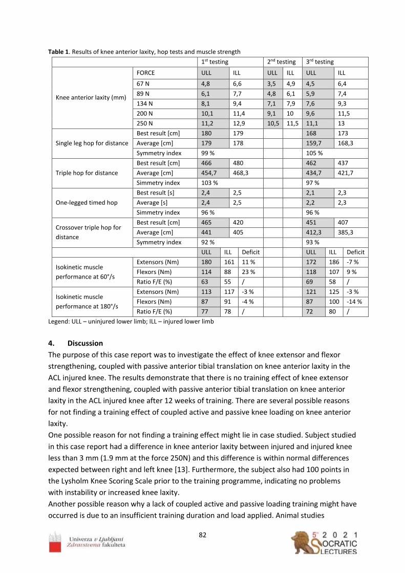
82
Table 1. Results of knee anterior laxity, hop tests and muscle strength
1st testing 2nd testing 3rd testing
Knee anterior laxity (mm)
FORCE ULL ILL ULL ILL ULL ILL
67 N 4,8 6,6 3,5 4,9 4,5 6,4
89 N 6,1 7,7 4,8 6,1 5,9 7,4
134 N 8,1 9,4 7,1 7,9 7,6 9,3
200 N 10,1 11,4 9,1 10 9,6 11,5
250 N 11,2 12,9 10,5 11,5 11,1 13
Single leg hop for distance
Best result [cm] 180 179 168 173
Average [cm] 179 178 159,7 168,3
Symmetry index 99 % 105 %
Triple hop for distance
Best result [cm] 466 480 462 437
Average [cm] 454,7 468,3 434,7 421,7
Simmetry index 103 % 97 %
One-legged timed hop
Best result [s] 2,4 2,5 2,1 2,3
Average [s] 2,4 2,5 2,2 2,3
Simmetry index 96 % 96 %
Crossover triple hop for
distance
Best result [cm] 465 420 451 407
Average [cm] 441 405 412,3 385,3
Symmetry index 92 % 93 %
ULL ILL Deficit ULL ILL Deficit
Isokinetic muscle
performance at 60°/s
Extensors (Nm) 180 161 11 % 172 186 -7 %
Flexors (Nm) 114 88 23 % 118 107 9 %
Ratio F/E (%) 63 55 / 69 58 /
Isokinetic muscle
performance at 180°/s
Extensors (Nm) 113 117 -3 % 121 125 -3 %
Flexors (Nm) 87 91 -4 % 87 100 -14 %
Ratio F/E (%) 77 78 / 72 80 /
Legend: ULL – uninjured lower limb; ILL – injured lower limb
4. Discussion
The purpose of this case report was to investigate the effect of knee extensor and flexor
strengthening, coupled with passive anterior tibial translation on knee anterior laxity in the
ACL injured knee. The results demonstrate that there is no training effect of knee extensor
and flexor strengthening, coupled with passive anterior tibial translation on knee anterior
laxity in the ACL injured knee after 12 weeks of training. There are several possible reasons
for not finding a training effect of coupled active and passive knee loading on knee anterior
laxity.
One possible reason for not finding a training effect might lie in case studied. Subject studied
in this case report had a difference in knee anterior laxity between injured and injured knee
less than 3 mm (1.9 mm at the force 250N) and this difference is within normal differences
expected between right and left knee [13]. Furthermore, the subject also had 100 points in
the Lysholm Knee Scoring Scale prior to the training programme, indicating no problems
with instability or increased knee laxity.
Another possible reason why a lack of coupled active and passive loading training might have
occurred is due to an insufficient training duration and load applied. Animal studies

83
investigating the response of connective tissues to load training, have used different
durations of training, with training programs lasting from 6 to 40 weeks [14-16]. Since the
duration of the training program in this case report was 12 weeks, it is possible that a
training duration was not long enough, or the effect of a delayed nature did occur but was
not found because of the lack of follow-up testing. Furthermore, we do not know accurately
the amount of load transferred to the ligament. We performed the dynamometer
measurement outside the knee joint and we can only speculate whether the measured load
(150N) was transferred to the ligament inside the knee joint and this load might not be
sufficient.
In addition, this case report was presented on a female patient. We are aware that female
patients are not an appropriate model for pilot trial on ligaments due to the menstrual cycle
significantly changing ligament strength. Future research is needed and should focus on
male subjects with increased knee anterior laxity as a consequence of ACL injury.
Acknowledgements
The authors acknowledge the financial support from the Slovenian Research Agency
(research core funding no. P3-0388).
References
1. Burroughs P, Dahners LE. The effect of enforced exercise on the healing of ligament
injuries. Am J Sports Med. 1990; 18: 376-378. doi: 10.1177/036354659001800407
2. Laros GS, Tipton CM, & Cooper RR. Influence of physical activity on ligament insertions
in knees of dogs. J Bone Joint Surg. 1971; 53A: 275-286.
3. Tipton CM, Vailas AC, Matthens RD. Experimental studies on the influences of physical
activity on ligament, tendons and joints: A brief review. Acta Med Scand Suppl 1986;
711: 157-168. doi: 10.1111/j.0954-6820.1986.tb08945.x
4. Woo SLY, Amiel D, Akeson WH, Kuei SC, Tipton CM. Effect of long-term exercise on
ligaments, tendons and bones of swine. Med Sci Sports Ex. 1979; 11: 105.
5. Woo SLY, Gomez MA, Woo YK, Akeson WH. Mechanical properties of tendons and
ligaments: the relationships of immobilization and exercise on tissue remodelling.
Biorheology. 1982; 19: 397-408. doi: 10.3233/bir-1982-19302
6. Woo SL, Abramowitch SD, Kilger R, Liang R. Biomechanics of knee ligaments: injury,
healing, and repair. J Biomech. 2006; 39:1-20. doi: 10.1016/j.jbiomech.2004.10.025
7. Kjaer M. Role of extracellular matrix in adaptation of tendon and skeletal muscle to
mechanical loading. Physiol Rev. 2004; 84: 649-698.
doi: 10.1152/physrev.00031.2003
8. Morrissey MC, Perry MC, King JB. Is knee laxity change after anterior cruciate ligament
injury and surgery related to knee extensor training load? Am J Phys Med Rehabil.
2009; 88: 369-375. doi: 10.1097/PHM.0b013e3181a0d7ed.

84
9. Barcellona MG, Morrissey MC, Milligan P, et al. The effect of knee extensor open
kinetic chain resistance training in the ACL-injured knee. Knee Surg Sports Traumatol
Arthrosc. 2015; 23:3168-3177. doi: 10.1007/s00167-014-3110-6.
10. Vauhnik R, Perme MP, Barcellona MG, et al. Robotic knee laxity testing: reliability and
normative data. Knee. 2013; 20: 250-255. doi: 10.1016/j.knee.2012.10.010
11. Lysholm J, Tegner Y. Knee injury rating scales. Acta Orthop. 2007; 78:445-53.
doi: 10.1080/17453670710014068
12. Barber SD, Noyes FR, Mangine R, DeMaio M. Rehabilitation after ACL reconstruction:
function testing. Orthopedics. 1992; 15(8): 969-74.
13. Daniel DM, Stone ML, Dobson BE, Fithian DC, Rossman DJ, Kaufman KR. Fate of the
ACL-injured patient. A prospective outcome study. Am J Sports Med. 1994; 22:632-644.
doi: 10.1177/036354659402200511
14. Cabaud HE, Chatty A, Gildengorini V, Feltman RJ. Exercise effects on the strength of the
rat anterior cruciate ligament. Am J Sports Med. 1980; 8: 79-86.
doi: 10.1177/036354658000800204
15. Sakuma K, Mizuta H, Takagi K. Effects of enforced exercise on biomechanical
properties of the anterior cruciate ligament in bipedal rats. J Japan Orthop Assoc 1992;
66: 1146-1155.
16. Vidik A. Elasticity and tensile strength of the anterior cruciate ligament in rabbits as
influenced by training. Acta Physiol Scand 1968; 74: 372-380. doi: 10.1111/j.1748-1716.1968.tb04245.x
85

86
_________________
Effect of repeated passive anterior loading on knee anterior laxity in injured
knee: A case report
Rugelj Darja1,2, Pilih Iztok3, VauhnikRenata1,2,3,* 1University of Ljubljana, Faculty of Health Sciences, Department of Physiotherapy, Slovenia 2Biomechanics Laboratory, Faculty of Health Sciences, University of Ljubljana, Slovenia 3Arthron, Institute for Joint and Sport Injuries, Slovenia
Abstract
It is believed that the only way to decrease knee joint laxity after anterior cruciate ligament
(ACL) injury, is with the surgical tightening of the knee. However, recent studies are
suggesting that low load open kinetic chain knee extensor exercises decrease knee anterior
laxity in ACL injured subjects. During this type of exercise, anterior directed load is placed on
the knee joint structures such as the ACL, which is the primary restraint of knee anterior
laxity. If anterior directed load is placed to the knee joint passively by knee arthrometer, a
decrease in knee anterior laxity might occur, since according to the mechanical properties,
ligaments are viscoelastic materials, designed especially to resist tensile forces. The purpose
was to evaluate the effect of repeated passive anterior loading on knee anterior laxity in the
injured knee. The partial anterior cruciate ligament tear was confirmed with MRI. We
performed repeated passive anterior loading with the GNRB® knee arthrometer. One loading
unit contained of 40 repetitions of anterior tibial translation at the force of 250N. We
performed passive anterior loading of the injured knee 3 to 5 times per week for a period of
20 weeks. Repeated passive anterior loading might decrease knee anterior laxity, however
future research is needed to define the appropriate duration and the amount of loading.
_________________

87
1. Introduction It is believed that the only way to decrease knee joint laxity after anterior cruciate ligament
(ACL) injury, is with the surgical tightening of the knee. Morrissey et al. (2009) [1] have found
that knee joint loading in ACL injured subjects can reduce knee anterior laxity. Similarly,
recent study by Barcellona et al. (2015) [2] suggested that low load open kinetic chain knee
extensor exercises decrease knee anterior laxity in ACL injured subjects. In these
investigations, loading was applied with open chain resistance exercise of the knee extensor
muscle group with knee anterior laxity reduced from this training. During this type of
exercise, anterior directed load is placed on the knee joint structures such as the ACL, which
is the primary restraint of knee anterior laxity. If anterior directed load is placed to the knee
joint passively by knee arthrometer, a decrease in knee anterior laxity might occur, since
according to the mechanical properties, ligaments are viscoelastic materials, designed
especially to resist tensile forces. In vitro animal studies have demonstrated the ability of the
knee medial collateral ligament complex to respond to mechanical loading (at loads that fall
within the linear region of the load-deformation response curve for that tissue), via an
increase in mechanical and ultrastructural properties such as ultimate load to failure,
stiffness and cross sectional area [3-6]. The purpose of our case report was to evaluate the
effect of repeated passive anterior loading on knee anterior laxity in the injured knee.
2. Methods Female subject 39 years old, with body height 156 cm and body mass 51 kg participated in
our case report. The partial ACL tear was confirmed with MRI and the ACL injury occurred a
year prior to participation in the study. Slovenia National Medical Ethics Committee (permit
No. 164/07/13) approved the study.
We performed passive anterior loading in the injured knee using GNRB® knee arthrometer.
GNRB® allows automated anterior tibial translation at force of 250N. In one loading unit, we
performed 40 repetitions of automated anterior tibial translation at force of 250N. We have
chosen the force of 250N, since this force is used to assess the integrity of the ACL with
GNRB® and since our previous work [7] of passive anterior loading done on uninjured knees
indicated that the force of 170N might not be large enough for changes to occur in knee
anterior laxity. We performed loading units from 3 to 5 times per week, for a period of 20
weeks. During the passive anterior loading of the knee, we have used EMG in order to detect
any hamstring activity (V-AMP 16; Brain products). Figure 1 presents the set up for the
loading unit.
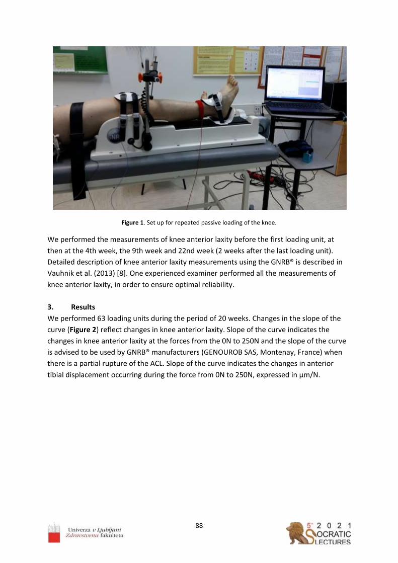
88
Figure 1. Set up for repeated passive loading of the knee.
We performed the measurements of knee anterior laxity before the first loading unit, at
then at the 4th week, the 9th week and 22nd week (2 weeks after the last loading unit).
Detailed description of knee anterior laxity measurements using the GNRB® is described in
Vauhnik et al. (2013) [8]. One experienced examiner performed all the measurements of
knee anterior laxity, in order to ensure optimal reliability.
3. Results
We performed 63 loading units during the period of 20 weeks. Changes in the slope of the
curve (Figure 2) reflect changes in knee anterior laxity. Slope of the curve indicates the
changes in knee anterior laxity at the forces from the 0N to 250N and the slope of the curve
is advised to be used by GNRB® manufacturers (GENOUROB SAS, Montenay, France) when
there is a partial rupture of the ACL. Slope of the curve indicates the changes in anterior
tibial displacement occurring during the force from 0N to 250N, expressed in μm/N.

89
Figure 2. Changes in knee anterior laxity after repeated passive anterior loading
At the first measurement of knee anterior laxity (before the loading units), the slope of the
curve was 40,6 μm/N. At the second measurement (4th week of loading) was 42.9 μm/N, at
the third measurement (9th week of loading) was 37.7 μm/N and at the fourth
measurement (22nd week (2 weeks after 20 weeks of loading)) was 44.8 μm/N, indicating
the changes in knee anterior laxity.
4. Discussion
The hypothesis tested in our case report was that repeated passive knee loading over a
number of weeks would decrease knee anterior laxity in the injured knee. The results
demonstrated that there was a decrease in knee anterior laxity in the injured knee observed
in the slope of the curve after the 8th weeks of repeated passive loading (42.9 μm/N vs 37.7
μm/N), however the knee anterior laxity increased then after 22 weeks, 2 weeks after 20
weeks of repeated passive loading. Since the slope of the curve after 22 weeks increased
compared to the slope of the curve at the first measurement (44.8 μm/N vs 40.6 μm/N), this
might indicate that passive anterior loading might increase knee anterior laxity.
For years, there is a debate in clinical and research areas, whether ACL injured subjects
should performed open kinetic chain exercises or no and whether the anterior loading of the
tibia is harmful or beneficial for ACL. Studies reports conflicting results. However, when
considering mechanical and structural properties of the ligaments, it is normal to conclude
that in order to make the ligament stronger, the proper loading must be applied and since
ligaments are responding to the tensile force, passive loading where tensile forces are
occurring in the ligament, would be a logical conclusion. Many animal studies have noted
that the forces being transmitted to ligaments and tendons will generally increase the
strength and functional capacity of these structures [3-6,9]. Mechanical loading therefore
plays a significant role in the maintenance and adaptation of the mechanical, ultrastructural,
histological and functional properties of connective tissues [10] via mechanotransduction
[11]. In vitro studies, knee medial collateral ligament complex responded to mechanical
1st week
4th week
9th week
22nd week
34
36
38
40
42
44
46
Slo
pe
of
the
curv
e (μm/N)
Weeks

90
loading (at loads that fall within the linear region of the load-deformation response curve for
that tissue), via an increase in mechanical and ultrastructural properties such as ultimate
load to failure, stiffness and cross sectional area [3-6]. In support of these animal studies,
Morrissey et al. (2009) [1] have proposed and Barcellona et al. (2015) [2] have found that
joint loading can reduce joint laxity. In these studies, loading was applied with resistance
open kinetic chain exercise of the knee extensor muscle group and knee anterior laxity
decreased from this training. These studies indicate that ligament might become stiffer,
which we suspect is due to soft tissue strengthening. Furthermore, recent study by Myrick et
al. (2019) [12] indicated that the mean volume of the anterior cruciate ligament significantly
increased from preseason to postseason among female collegiate athletes, indicating that
physical demand of sport activities influence knee laxity. Loading can have contrasting,
intensity-related effects. For example in bone, loading can be both beneficial and harmful,
depending on intensity [13]. Therefore, the possibility exists that lesser amounts of passive
joint loading may stimulate targeted tissues to increase their strength and this increased
strength may result in enhancing the tissue's ability to resist loads thereby maintaining joint
stability. In our case report, the laxity decreased after 8 weeks of passive anterior loading,
but then the laxity increased and it might be that the duration of tensile loading more than 8
weeks is not beneficial for decreasing the knee anterior laxity in humans. Animal studies,
investigating the response of ligaments to loading, have used different durations of training
programs, with training programs lasting from 6 to 40 weeks [14-16]. Furthermore, maybe
the next step is to combine active and passive knee (ligament) loading. Future research is
warranted in order to confirm what kind of loading is beneficial for the ACL ligament in
terms of the amount of force, number of repetitions and duration.
Acknowledgements
The authors acknowledge the financial support from the Slovenian Research Agency
(research core funding no. P3-0388).
References
1. Morrissey MC, Perry MC, King JB. Is knee laxity change after anterior cruciate ligament
injury and surgery related to knee extensor training load? Am J Phys Med Rehabil.
2009; 88: 369-375. doi: 10.1097/PHM.0b013e3181a0d7ed
2. Barcellona MG, Morrissey MC, Milligan P, et al. The effect of knee extensor open
kinetic chain resistance training in the ACL-injured knee. Knee Surg Sports Traumatol
Arthrosc. 2015; 23:3168-3177. doi: 10.1007/s00167-014-3110-6
3. Laros GS, Tipton CM, Cooper RR. Influence of physical activity on ligament insertions in
knees of dogs. J Bone Joint Surg. 1971; 53A: 275-286.
4. Woo SLY, Amiel D, Akeson WH, et al. Effect of long-term exercise on ligaments,
tendons and bones of swine. Med Sci Sports Ex. 1979; 11: 105.

91
5. Woo SLY, Gomez MA, Woo YK, Akeson WH. Mechanical properties of tendons and
ligaments: the relationships of immobilization and exercise on tissue remodelling.
Biorheology. 1982; 19: 397-408. doi: 10.3233/bir-1982-19302
6. Burroughs P and Dahners LE. The effect of enforced exercise on the healing of ligament
injuries. Am J Sports Med. 1990; 18: 376-378. doi: 10.1177/036354659001800407
7. Vauhnik R, Perme MP, Barcellona MG, et al. Effect of repeated passive anterior loading
on human knee anterior laxity. Man Ther. 2015; 20:709-714.
doi: 10.1016/j.math.2015.02.007
8. Vauhnik R, Perme MP, Barcellona MG, et al. Robotic knee laxity testing: reliability and
normative data. Knee. 2013; 20: 250-255. doi: 10.1016/j.knee.2012.10.010
9. Tipton CM, Vailas AC, Matthens RD. Experimental studies on the influences of physical
activity on ligament, tendons and joints: A brief review. Acta Med Scand Suppl. 1986;
711: 157-168. doi: 10.1111/j.0954-6820.1986.tb08945.x
10. Woo SL, Abramowitch SD, Kilger R, Liang R. Biomechanics of knee ligaments: injury,
healing, and repair. J Biomech. 2006; 39:1-20. doi: 10.1016/j.jbiomech.2004.10.025
11. Kjaer M. Role of extracellular matrix in adaptation of tendon and skeletal muscle to
mechanical loading. Physiol Rev. 2004; 84: 649-698. doi: 10.1152/physrev.00031.2003
12. Myrick KM, Voss A, Feinn RS, Martin T, Mele BM, Garbalosa JC. Effects of season long
participation on ACL volume in female intercollegiate soccer athletes. J Exp Orthop.
2019; 6-12. doi: 10.1186/s40634-019-0182-8
13. Guadalupe-Grau A, Fuentes T, Guerra B, Calbet JA. Exercise and bone mass in adults.
Sports Med. 2009; 6: 439-468. doi: 10.2165/00007256-200939060-00002
14. Sakuma K, Mizuta H, Takagi K. Effects of enforced exercise on biomechanical
properties of the anterior cruciate ligament in bipedal rats. J Japan Orthop Assoc.
1992; 66: 1146-1155.
15. Cabaud HE, Chatty A, Gildengorini V, Feltman RJ. Exercise effects on the strength of the
rat anterior cruciate ligament. Am J Sports Med. 1980; 8: 79-86.
doi: 10.1177/036354658000800204
17. Vidik A. Elasticity and tensile strength of the anterior cruciate ligament in rabbits as
influenced by training. Acta Physiol Scand. 1968; 74: 372-380.
doi: 10.1111/j.1748-1716.1968.tb04245.x

92

93
_________________
Extraction of polyethylene terephthalate (PET) microplastics from alluvial soil:
comparison of density separation and oil-based extraction
Leban Pia1,*,Bavcon Kralj Mojca1, Griessler Bulc Tjaša1, Prosenc Franja2,** 1University of Ljubljana, Faculty of Health Sciences, Department for Sanitary Engineering,
Ljubljana, Slovenia 2University of Ljubljana, Faculty of Health Sciences, Research Institute, Ljubljana, Slovenia
Abstract
Microplastics (MPs) have become a global environmental problem, with high occurrence in
marine and terrestrial environments. Research of MPs in soil and other organic-rich matrices
has become important in recent years, but methods for extraction, analytical methods for
quantification and identification of MPs have not yet been standardised. Two methods for
extraction of MPs from alluvial soil were compared, oil-based extraction and density
separation method. The recovery of the extracted MPs in both methods was higher than
90 %, with 97 ± 8 % (10 PET MPs per 10 g of soil) and 98 ± 3 % (20 PET MPs per 10 g of soil)
obtained using oil-based extraction, and with 93 ± 5 % (10 PET MPs per 10 g of soil) and
99 ± 2 % (20 PET MPs per 10 g of soil) for density separation method. In further research,
the two extraction methods will be tested on different MP polymers, as well as soils with
varying organic content. The optimal protocol will then be used to extract MPs from
environmental samples for further quantification and identification.
_________________

94
1. Introduction
Plastic is stable and widely applied material with intensive production worldwide, causing a
large amount of plastic waste, where almost 90 % of it ends up directly or indirectly in
terrestrial environment [1]. Plastics can enter terrestrial environment through littering and
street runoff (containing tire wear). Other pathways are atmospheric deposition,
wastewater irrigation, mulching film and application of biosolids, compost, and sewage
sludge as fertiliser [2-5]. With different natural processes, such as weathering, mechanical
wear, hydrolysis and others, plastic breaks down into countless small particles. Some of
those particles are microplastics (MPs), which are smaller than 5 mm. MPs represent a great
risk to the environment and also to the human health, because they can easily transport to
different environmental media, they can be ingested by organisms and may enter the food
chain [1]. They can also carry different hazardous substances, such as hydrophobic organic
pollutants and pesticides [6]. With high occurrence and lack of analytical methods for
quantification and identification, MPs have become and will remain a global environmental
problem [1].
Polyethylene terephthalate (PET) is a commonly and widely used polymer, usually intended
for packaging, often plastic bottles as well as clothing. It is produced by the polymerisation
of ethylene glycol and terephthalic acid [7]. PET is classified as high and low-density polymer.
The density of semi-crystalline high-density PET is between 1.37 and 1.40 g cm-3 and the
melting point is in the 255–265 °C temperature range [8]. It can be found as MPs almost
everywhere, in water, soil, compost and sewage sludge [4,5]. The method for extraction and
quantification of MPs from soil has not yet been standardised and presents multiple
challenges due to the complexity of the medium and the presence of organic matter [3].
In this study, two methods for MP extraction, made from the model polymer PET, from
alluvial soil samples were compared. The oil-based extraction, which takes advantage of the
lipophilic surface properties of most plastics, and a commonly used density separation
method, which separates MPs from soil, based on the density difference of MPs and the
saline solution were studied [9,10].
2. Methods
2.1 PET MP particle preparation
Two methods were tested on the alluvial soil and spiked with particles of the high-density PET
polymer. Square pieces of PET plastics were cut manually in the dimension range from 0.1 to
2 mm, as shown in Figure 1.

95
Figure 1. Manually prepared polyethylene terephthalate (PET) microplastic particles.
2.2 Oil-based extraction
The oil-based extraction method was tested on alluvial soil samples, spiked with PET MPs in
different quantities. For this method, a custom-made polytetrafluoroethylene (PTFE)
cylinder was made. In it, 10 g of alluvial soil was mixed with a defined number of PET MP
particles (10 and 20), 10 mL of distilled water and 3 mL of olive oil. Firstly, the closed cylinder
was shaken, then left settling for 2 h and finally put into the freezer overnight. Once frozen,
the sample was pushed out of a cylinder with a piston and the oil layer was separated from
the rest of the ice. The frozen oil layer, containing MPs was left to thaw on a glass fibre filter
(Whatman GF/C 47 mm) and then filtered through and rinsed with water and subsequently
with hexane to remove traces of oil. This protocol, shown in Figure 2, was adapted with
changes from Scopetani et al. (2020) [10].
Figure 2. The oil-based extraction method procedure; a: sedimentation step, b: the sample of alluvial soil and 10
PET MP particles (marked with red circles) on a glass fibre filter.
cm

96
2.3 Density separation
The density separation method was tested on alluvial soil sample, spiked with PET MPs in
different quantities. The extraction was done in a centrifugation tube, as follows: 10 g of
alluvial soil was mixed with a defined number of PET MP particles (10 and 20) and 50 mL of
ZnCl2 solution (ρ= 1.6 g cm-3) were added to the tube. Firstly, the closed centrifugation tube
was shaken, then put in a centrifuge (Hettich, UNIVERSAL 320) for 30 minutes at 5500 rpm.
The supernatant was gently removed from the centrifugation tube, filtered through a glass
fibre filter, and rinsed with distilled water. This protocol, shown in Figure 3, was adapted
with changes from Konechnaya et al. (2020) [9], considering speeding up the settling with
the use of a centrifuge [11].
Figure 3. The density separation method procedure; a: centrifugate tubes with samples after centrifugation, b: filtration and recycling the ZnCl2 solution.
2.4 Quantification of extracted MPs After both extraction procedures, samples on the glass fibre filters were left to air dry and MPs were then manually quantified. Recovery was calculated as follows:
𝑅𝑒𝑐𝑜𝑣𝑒𝑟𝑦 (%) = 𝑁𝑒𝑥𝑡𝑟𝑎𝑐𝑡𝑒𝑑
𝑁𝑠𝑝𝑖𝑘𝑒𝑑× 100 (1)
3. Results
a. Oil-based extraction
Based on a literature review of various oil-based extraction protocols and on the empirical
experiences gained in the presented research, several advantages and disadvantages of the
method were identified [10,12-14] as reported in Table 1.

97
Table 1. Advantages and disadvantages of oil-based extraction method.
Advantages Disadvantages
Safe and cheap method Time consuming (at least 12 h) (Scopetani et al., 2020)[11]
Custom made equipment needed (Scopetani et al., 2020) [11]
No hazardous saline solutions Using foodstuffs (olive oil)
Highly applicative to different polymer types (Scopetani et al., 2020)[11]
Required removal of oil traces (with hexane) (Scopetani et al., 2020)[11]
Require an additional step to remove organic substances from a sample
Highly applicative to various soil
types and mixtures
Low repeatability in real samples (He et al., 2020)[14]
Co-adhesion of contaminants to MPs surface (He et al., 2020)[14]
Table 2. Differences in experimental design between this and other studies.
Study Polymer type Size and shape Number of MP in sample
Matrix used Oil
Crichton et al., 2017 [12]
Expanded polystyrene (EPS) Polyvinyl chloride (PVC) Acrylonitrile butadiene styrene (ABS) Vinyl Polyamide (PA) Polyester (PES) Nylon
Particles (minimum 0.43 mm width and maximum 6.17 mm length) Fibers (minimum 0.1 mm width and maximum 20.81 mm length)
Spiked in environmental samples 10 particles of each polymer type added (60 in total) per sample (50 g of sediment)
Medium-grained sediment
Canola oil
Mani et al., 2019 [13]
Polystyrene (PS) Polypropylene (PP) Polymethyl methacrylate (PMMA) Glycol modified polyethylene terephthalate (PET)
Particles Mechanically fragmented and sieved into small (0.3–0.5 mm) and large (0.5–1.0 mm) fractions
100 MP particles (15 small and 10 large fragments of each polymer type) added per sample (1.0 g for FSS and MSS and 10.0 g for MBS and AS)
Marine suspended surface solids (MSS) Fluvial suspended surface solids (FSS) Marine beach sediments (MBS) Agricultural soil (AS)
Castor oil
Scopetani et al., 2020 [10]
Polyethylene (PE) Polyurethane (PU) Polystyrene (PS) Polycarbonate (PC) Polyvinyl chloride (PVC) Polyethylene terephthalate (PET)
Mechanically fragmented particles 0.2 – 2 mm
60 MP particles (10 particles of each polymer type) added per sample (25 g of soil and 10 g of compost)
Soil Compost
Olive oil
This study Polyethylene terephthalate (PET)
Mechanically fragmented particles 0.1 – 2 mm
10 or 20 MP particles added per sample (10 g of soil)
Alluvial soil Olive oil

98
The MPs recovery rate reported in the literature was on average 95 ± 4 % [10,12,13]. Our oil-
based extraction method recovery rate was 97 % ± 8 % and 98 % ± 3 % for 10 and 20 PET MP
particles, respectively. The recovery obtained in this study is higher than in the reported
literature, however, some important differences in the experimental design between this
and other studies exist and are shown in Table 2.
b. Density separation
With a literature review of various density separation protocols as well as the empirical experience gained in this study, several advantages and disadvantages of the method were identified [3,9,11,14,15] as shown in Table 3 below. Table 3. Advantages and disadvantages of density separation method.
Advantages Disadvantages
Simply applicable method Expensive saturated saline solutions
High density range Hazardous solutions (NaI, ZnCl2, ZnBr2 toxic and corrosive salts) [12,14,16]
Saline solution can be recycled and reused
Highly applicative to different polymer
types [15] Reactive extraction solution (CaCl2, ZnCl2) [3]
Highly applicative to various soil types and
mixtures
Different for low-/high-density MPs [14]
Require an additional step to remove organic substances from a sample
Time-efficient (cca. 4 samples per hour)
On average, the recovery rates mostly ranged between 94 % and 97 % with standard
deviation (SD) between 0.3 % and 3.3 % with decreasing particle size [9,11,15]. The recovery
rate obtained in this study was 93 ± 5 % and 99 ± 2 % 10 and 20 PET MPs, respectively.. The
recovery rate obtained in this study is in agreement with the reported literature, however,
some important differences in experimental design between this and other studies exist and
are shown in Table 4.

99
Table 4. Differences in experimental design between this and other studies.
Study Polymer type Size and shape
Number of MP in sample
Matrix used
Density separation
Konechnaya et al., 2020 [9]
Polyethylene (PE) Polypropylene (PP) Polyvinyl chloride (PVC) Polystyrene (PS) Polyethylene terephthalate (PET) Polymethyl methacrylate (PMMA) Polyurethan (PU) Polyamide (PA)
Particles Grain size fractions of 1-5 mm, 400-
1,000 µm,
200-400 µm and 100-200 µm
0.5 g of each grain size fraction of each polymer particles per sample (10 g of sea sand)
Precleaned calcinated sea sand
Stirring (3x for 2 min) Sedimentation (10 minutes) Floatation ZnCl2 solution
Vermeiren et al., 2020 [11]
Polyethylene (PE) Polypropylene (PP) Polystyrene (PS) Expanded polystyrene (EPS) Polyethylene terephthalate (PET) Nylon (PA) Polyvinyl chloride (PVC)
Mechanically fragmented particles 0.16 – 12.13 mm
60 mL of sediment was then spiked with different sized MP of different polymers
Sediment: Low intertidal mudflat High intertidal mudflat Saltmarsh (Phragmites australis)
Overflow column with top inflow Stirring (5 min followed by 5 min rest and three short stirring bursts) Sedimentation (24 h) Floatation ZnCl2 solution
This study Polyethylene terephthalate (PET)
Mechanically fragmented particles 0.1 – 2 mm
10 or 20 MP particles added per sample (10 g of soil)
Alluvial soil
Centrifugation 30 minutes at 5500 rpm Floatation ZnCl2 solution
3.3 Comparison of the two extraction methods
In terms of recovery, the two extraction methods were comparable, however, the density separation method yielded better recovery rate for 20 PET MPs than the oil-based extraction. For extraction of 10 PET MPs, the oil-based extraction was slightly better than density separation method, as shown in Figure 4. The variability of measurements (shown as SD values on the graph) were lower for density separation method for both, 10 and 20 PET MPs, making density separation a more replicable method.

100
Figure 4. Oil extraction and density separation from alluvial soil recovery rates (%) of 10 and 20 PET MPs (N=6).
4. Discussion
Both extraction methods have proven advantages and disadvantages in terms of cost, time
effectiveness and material safety.
Oil-based extraction is a safe and cheap method, which does not use any hazardous saline
solution. It is highly applicative to different polymer, such as PE, PU, PS, etc. and soil types,
such as compost and agricultural soil [10]. On the other hand, it is time consuming due to
the overnight freezing process and subsequent thawing. It also requires a custom-made
equipment (PTFE cylinder and a piston). An oil layer frequently formed on the cylinder’s wall,
where the MP particles got trapped and had to be washed off the inner walls. Moreover, the
PET MP particles also tended to stick to the outside of the frozen sample cylinder and had to
be, therefore, scraped from the surface of the frozen sample. Furthermore, this method,
albeit in small quantities, uses foodstuff. Before further analysis, removal of oil traces with
hexane is required [10]. Oil-based extraction method efficiency and accuracy vary due to
different properties of environmental samples. Lipophilic properties of plastic polymers may
also be modified, due to contaminants adhered to the surface of MPs [14].
Density separation method is a simple method and easily applicable in the laboratory. Saline
solutions with sufficiently high density can cover a wide range of different MP polymers,
from low to high-density polymers, and is, therefore, highly applicable to different polymer
and soil types [14,15]. The density of ZnCl2 solution has not changed after the first filtration,
therefore, ZnCl2 solution can be recycled to be used in further filtration processes. However,
the preparation of saturated saline solutionrequires large quantities of a chosen salt, which
makes density separation method expensive. In our study, 1 kg of ZnCl2 salt was used to
prepare 1.2 L of saturated solution with density of1.6 g cm- 3. Saline solutions for density
separation method (NaI, ZnCl2, ZnBr2) are toxic and corrosive salts, hazardous to the
environment, and what is more, highly reactive. Möller et al. (2020)[3] reported that ZnCl2

101
solution can react with natural components of the sediment, especially with carbonates
(resulting in bubbling and foam), which can hamper the procedure, however, no such thing
had occurred in our samples when ZnCl2 was used. Literature reports that low-density MPs
can be more easily extracted than high-density MPs [14], however, PET is at the high-end of
density of plastic polymers (1.38 g cm- 3), and the recoveries obtained in this study show
otherwise.
Both methods require an additional step to remove or decrease organic content from a
sample, especially for soil samples rich in organic matter (agricultural soil, compost and soil-
compost mixtures). This step was not required in our study since alluvial soil is poor in
organic matter content (2.30 ± 0.13 %).
Recovery obtained with both extraction methods in this study was better or in the similar
range as the one reported in the literature. It should be noted, however, that experimental
designs (e.g., number and size of MPs used, environmental matrices used) was different in
different studies, therefore, comparison of recovery rates is not straightforward.
Currently, oil extraction method appears to be safer for the environment, however, density
separation method is more time efficient, is easier to handle and ZnCl2 solution can be
recycled and reused again. Density separation method is able to achieve slightly higher
recovery rates and lower variability. By optimising and testing both methods on a wide range
of different polymer types, concentrations and sizes of MPs and different matrices with
varying organic matter content in comparable experimental designs, we will be able to
determine which method is more suitable and yields better recoveries.
Further work will focus on quantification and identification of microplastics in real
environmental samples, such as agricultural soil, bio-waste compost, sludge from
wastewater treatment plants and others.
Acknowledgements
This work was supported by the Slovenian Research Agency, research core funding No. P3-
0388 (Mechanisms of Health Maintenance), and research project No. Z2-2643 (Agri-iMPact:
Microplastic Prevalence and Impact in Agricultural Fields).
References 1. Zhou Y, Wang J, Zou M, Jia Z, Zhou S, Microplastics in soils: A review of methods,
occurrence, fate, transport, ecological and environmental risks. Sci Total Environ. 2020;
748: 141368. doi: 10.1016/j.scitotenv.2020.141368
2. Kumar M, Xiong X, He M, et al. Microplastics as pollutants in agricultural soils. Environ
Pollut. 2020; 265: 114980. doi: 10.1016/j.envpol.2020.114980
3. Möller J N, Löder M G, Laforsch C, Finding microplastics in soils: A review of analytical
methods. Environ Sci Technol. 2020; 54(4): 2078-2090. doi: 10.1021/acs.est.9b04618
4. Müller A, Goedecke C, Eisentraut P, Piechotta C, Braun U, Microplastic analysis using
chemical extraction followed by LC-UV analysis: a straightforward approach to
determine PET content in environmental samples. Environ Sci Eur. 2020; 32(85): 1-10.
doi: 10.1186/s12302-020-00358-x

102
5. Wang C, Zhao J, Xing B, Environmental Source, Fate, and Toxicity of Microplastics. J
Hazard Mater. 2021; 407: 124357. doi: 10.1016/j.jhazmat.2020.124357
6. Šunta U, Prosenc F, Trebše Polonca, Griessler Bulc Tjaša, Bavcon Kralj M. Adsorption of
acetamiprid, chlorantraniliprole and flubendiamide on different type of microplastics
present in alluvial soil. Chemosphere. 2020; 261: 1-9,
doi:10.1016/j.chemosphere.2020.127762
7. Britannica, T. Editors of Encyclopaedia (2020), Polyethylene terephthalate
[Encyclopedia Britannica], Accessed 29. 1. 2021. Available from
https://www.britannica.com/science/polyethylene-terephthalate
8. Nisticò R, Polyethylene terephthalate (PET) in the packaging industry. Polym Test.
2020; 90: 106707. doi: 10.1016/j.polymertesting.2020.106707
9. Konechnaya O, Lüchtrath S, Dsikowitzky L, Schwarzbauer J, Optimized microplastic
analysis based on size fractionation, density separation and μ-FTIR. Water Sci Technol.
2020; 81(4): 834-844. doi: 10.2166/wst.2020.173
10. Scopetani C, Chelazzi D, Mikola J, et al. Olive oil-based method for the extraction,
quantification and identification of microplastics in soil and compost samples. Sci Total
Environ. 2020; 733: 139338. doi: 10.1016/j.scitotenv.2020.139338
11. Vermeiren P, Muñoz C, Ikejima K, Microplastic identification and quantification from
organic rich sediments: A validated laboratory protocol. Environ Pollut. 2020; 262:
114298. doi: 10.1016/j.envpol.2020.114298
12. Crichton E M, Noël M, Gies E A, Ross P S, A novel, density-independent and FTIR-
compatible approach for the rapid extraction of microplastics from aquatic sediments.
Anal Methods. 2017; 9(9): 1419-1428. doi: 10.1039/C6AY02733D
13. Mani T, Frehland S, Kalberer A, Burkhardt-Holm P, Using castor oil to separate
microplastics from four different environmental matrices. Anal Methods. 2019; 11(13):
1788-1794. doi: 10.1039/C8AY02559B
14. He D, Zhang X, Hu J, Methods for separating microplastics from complex solid matrices:
Comparative analysis. J Hazard Mater. 2021; 409:124640.
doi: 10.1016/j.jhazmat.2020.124640
15. Li J, Song Y, Cai Y, Focus topics on microplastics in soil: analytical methods, occurrence,
transport, and ecological risks. Environ Pollut. 2020; 257: 113570.
doi: 10.1016/j.envpol.2019.113570
16. Scheurer M, Bigalke M, Microplastics in Swiss Floodplain Soils. Environ Sci Technol.
2018; 52(6): 3591−3598. doi: 10.1021/acs.est.7b0600

103

104
_________________
European spruce (Picea abies) as a possible sustainable source of cellular
vesicles and biologically active compounds
Jeran Marko1,2,*, Božič Darja1,2, Novak Urban3, Hočevar Matej4, Romolo Anna1, Iglič Aleš2,
Kralj-Iglič Veronika1
1University of Ljubljana, Faculty of Health Sciences, Laboratory of Clinical Biophysics,
Ljubljana, Slovenia 2University of Ljubljana, Faculty of Electrical Engineering, Laboratory of Physics, Ljubljana,
Slovenia 3National Institute of Chemistry, Laboratory for Biomolecular Structure, Ljubljana, Slovenia 4Institute of Metals and Technology, Physics and Chemistry of Materials, Ljubljana, Slovenia
Abstract
Cells secrete different types of particles into the extracellular space. Cellular vesicles (CVs)
are such particles that span in size downto 30 nm. CVs have been found to be involved in
various applications. Research of the formation of naturally formed CVs dates back to 1960.
The main motivation of this work is study of processes to develop large-scale production of
vesicles, which requires simple, robust, and inexpensive methods. We focused on processing
European spruce needles, which represent a "green" source of various natural organic
compounds and cellular particles. CVs were isolated from spruce needle macerates of raw,
ultrasound-treated and lecithin –treated samples by centrifugation and characterized by
microscopy (light and scanning electron (SEM) technique), flow cytometry and Fourier
Transform IR spectroscopy (FTIR). We found that macerates contained CVs of different sizes,
that CVs were formed also during processing of samples and that the concentration and the
size of CVs in isolates depended on the centripetal acceleration of the centrifuge rotor.
_________________

105
1. Introduction
Cells secrete different kinds of small particles into the extracellular space. Cellular vesicles
(CVs) are such particles that are enclosed by biomembranes. Their size extends downto
about 30 nm. It was found that CVs are involved in the horizontal transfer of cargoes,
especially nucleic acids (DNA, mRNA and microRNA) and other molecules such as
carbohydrates, lipids and secondary metabolites [1,2]. Due to these properties, CVs are
considered as mediators of cell-to-cell communication and exhibit important functions in
different physiological and pato-physiological processes; for example they are enroled in
signal transduction, cell cycle, immune response, neurological diseases, inflammation and
tumorigenesis [2]. Recently, the demands for large-scale production of vesicles has been
recognized and simple, robust, and inexpensive methods are required.
CVs are being studied in different systems, including plants [3]. Already in the sixties,
Halperin and Jensen (1967) studied embryogenesis in cell cultures derived from the wild
carrot (Daucus carota) [3,4]. By using transmission electron microscopy they observed CVs
within multivesicular bodies which seemed to fuse with the cell membrane and release the
cargo of secondary vesicles into the wall space [4]. Also they reported of smooth
endoplasmatic reticulum containing small vesicles similar to the vesicles seen in
multivesicular bodies [4].
Ultracentrifugation-based isolation methods for CVs were developed [3,6]. Low centrifugal
accelerations (cca 500 × g) were used to pellet cellular debris from macerates, followed by
higher centrifugal accelerations (cca 10 000 × g) to pellet CVs from supernatant of the first
centrifugation step [3,6]. Gradient centrifugation methods were also applied to fractionate
the samples according to the density of CVs [3]. Ju et al., (2013) isolated grape exosome-like
nanoparticles (GELNs) from grape juice using differential centrifugation and sucrose gradient
method [7]. Cryogenic electronic microscope images of a particular CV fraction of the isolate
revealed numerous vesicles with diameters between 50 and 300 nm [3,7]. Later, several
studies reported the presence of CVs in many different plant sources; e.g. in the germination
medium of olive pollen grains, in the extracellular fluid of sunflower seedlings, in coconut
milk and others [3].
Plants have the incredible ability to synthesize many of the active compounds on which
today’s drugs and therapies are based. They are able to defend themselves against external
influences (enemies) by releasing the appropriate molecules in different body parts [8]. One
of them is the European spruce (Picea abies), which is a widespread and common tree [9].
Different parts of spruce tree contain different mixtures of complex biologically active
substances. The presence and concentration of these substances in a given plant depends on
several factors (e.g. climate, time of collection in the year, accessibility to nutrients, etc.) [8].
Large-scale production of vesicles requires simple, robust, and inexpensive methods.
As phospholipid molecules form vesicles in aqueous media, we expected that their addition
to the macerate would involve them in formation of mixed vesicles. We expected that
vesicles will be forming during maceration of spruce needles.

106
Sonication can induce disruption of cell walls and membranes and is often used to improve
efficiency of isolation of active ingredients (compounds) from natural sources. Combined
with sequential extraction steps using different solvents, ultrasonic disintegration has been
shown to be effective in separating and/or resolving various natural compounds [10]. To
increase the production of CVs from plant tissues, ultrasonication (US) was used as a
pretreatment for the isolation of CVs in this study.
We report preliminary results on CVs isolated from a macerate of needles of European
spruce. We have isolated CVs by centrifugation and analyzed them by flow cytometry, FTIR
spectroscopy and scanning electron microscopy (SEM).
2. Materials and Methods
2.1. Plant material and its preparation
Branches of spruce were cut from the tree and used immediately. Branches were immersed
into 1.5 L of water at 30 oC with dissolved sodium hypochlorite (NaClO, 0.1 %) for 1 hour. The
branches were rinsed with water. The needles were cut off from the branches. Macerate
was prepared from 50 g of needles and 300 mL of 0.9 % saline solution by stirring for about
20 seconds with the stick hand mixer, (HBC804QW, Gorenje, Velenje, Slovenia). To prepare
the CVs with addition of lecithin, 5 g of lecithin granules were added to the sample during
the stirring. After maceration, larger parts were removed from the sample by filtering
through a sterile gauze. The filtered sample was left in closed sterile plastic 50 mL containers
to sediment for 2 hours while the supernatant (of almost equal volume) was used for further
processing.
2.2. Sonication of macerate
In 50 mL or 15 mL conical plastic centrifuge tubes (Isolab, Germany), the sap sample (plant
material in saline) was added and sonicated in “sweep” mode for 5 min at 37 kHz at room
temperature (ultrasonic bath Elma S 100 H, Germany).
2.3. Isolation of CVs
CVs were isolated by centrifugation as schematically depicted in Figure 1. The sample was
aliquoted in 50 mL or 15 mL conical plastic centrifuge tubes (Isolab, Germany). The aliquots
were centrifuged for 10 minutes at 300 × g and 5 oC in the Centric 400R centrifuge (Domel,
Železniki, Slovenia) equipped with the swinging rotor. After pelleting larger particles, the
supernatant was centrifuged for 30 minutes at 2000 × g and 5 oC to sediment possibly
present bacteria. The supernatant was further centrifuged for 60 minutes at 10000 × g or
17500 × g in the Centric 200R centrifuge (Domel, Železniki, Slovenia) with the Lilliput
swinging rotor or for 60 minutes at 50 000 × g at 5 oC with the L8-70M ultracentrifuge
(Beckman Coulter, USA, rotor type SW55Ti).

107
Figure 1: Flowchart of the experimental design for isolation of CVs by centrifugation.
2.4. Flow cytometry (FCM)
FCM measurements were performed using MACS QUANT flow cytometer (Miltenyi,
Bergisch-Gladbach, Germany), with lasers set at 458 V (FSC), 467 V (SSC), and the trigger set
at SSC: 1.8. Particles in fresh isolates were analyzed by flow cytometry immediately after
isolation. Gates were set based on analysis of standard beads of size 2 and 3 µm
(MACSQuant Calibration Beads, Ref: 130-093-607) (Figure 2A). A representative scatterplot
pertaining to the isolate is presented in Figure 2B.
Figure 2. Flow cytometer scatter plots of: (A) standard beads of size 2 and 3 µm – MACSQuant Calibration Beads
and (B) a representative sample of the supernatant after centrifugation for 30 minutes at 2000 × g.
2.5. Fourier Transform IR spectroscopy (FTIR)
The FTIR spectra were measured using the Bruker Vertex 80 FTIR spectrometer. We
employed Specac’s Golden gate ATR cell with diamond crystal and heated top plate. Spectra
were recorded in the range between 4000 and 600 cm-1. The final spectrum was averaged
from 128 interferograms. Before any spectral analysis, the spectrum of pure buffer was
subtracted. ATR absorbance spectra were used as recorded without post-processing due to
reflection contributions to the overall absorbance spectra. Subtracted spectra were

108
integrated in two separate regions. The first region (3000–2850 cm-1) corresponds to CH2
and CH3 stretching vibrations of fatty acids. Meanwhile, the second region (1180–960 cm-1)
corresponds to C-O and C-C stretching vibrations in combination with C-O-H, C-O-C
deformation vibrations of carbohydrates [11]. Finally, the ratio between integrated areas of
the first and the second spectra region was calculated.
2.6. Scanning electron microscopy (SEM)
The samples were fixed with OsO4, following a modified protocol adopted from Božič, et al
[12]. The pellets and the starting material (saline macerate of the plant material) were fixed
on 0.05-micron mixed-cellulose-esters’ filters (Sterlitech, USA).
Samples were incubated in 1% OsO4 for 2 h, washed 3 times with distilled water (incubation
time 10 min each), then dehydrated in graded series of ethanol (30%, 50%, 70%, 80%, 90%
and “absolute”, 10 min each; absolute ethanol was replaced 2 times) and
hexamethyldisilazane (mixed with absolute ethanol; 30%, 50% and "absolute", 10 min each)
and finally air dried. Samples were coated with Au/Pd (PECS Gatan 682) and analyzed using a
JSM-6500F Field Emission Scanning Electron Microscope (JEOL Ltd., Tokyo, Japan).
3. Results and Discussion
3.1. Visualization of samples
During the maceration, samples produced foam (Figure 3) indicating presence of
membranous structures in the samples.
Figure 3. Foam formed during maceration.
Light microscopy of the foam collected from the top of the macerate revealed giant colloid
vesicles in raw samples and in lecithin-treated sample (Figure 4A and B, respectively). Pellet
after centrifugation at 300g of the raw sample and supernatant after sedimentation of the
macerate in gravity field of the lecithin-treated sample exhibited numerous particles with
smooth contours (Figure 4C,D), heterogeneous in size. As internal structures are not
recognized, and due to the size of these particles (of the order of several m) these particles
could be cell remnants (empty cell walls, or smaller colloid vesicles). There were also
numerous smaller particles, heterogeneous in size and shape that tended to form clusters
(Figure 4C,D). Figure 4E shows supernatant of raw sample after centrifugation at 2000g with

109
numerous particles of which some have shapes of minimal membrane free energy
characteristic for membrane – enclosed particles without internal structure [13] – i.e. CVs
(Figure 4E). Giant vesicles of lecithin in saline are shown for comparison (Figure 4F).
Visualization of macerates by SEM revealed remnants of cells (white arrows), amorphous
material and sub-micrometer-sized particles (yellow arrows) which were more abundant in
the samples prepared by addition of lecithin (Figures 5A and 5C, respectively). Also isolates
(Figures 5B and 5D) contained sub-micron-sized particles with smooth contours. The
morphology of particles in samples seemed similar in supernatants and pellets, however,
with varying sizes and concentrations.
Figure 4: Visualization of European spruce macerate and isolate of CVs by light microscopy. A: Lecithin in 0.9%
saline solution, B: spruce needle macerate with addition of lecithin, foam phase, C: supernatant of
sedimentation of the filtered macerate in gravitational field, D: pellet of the sample C after centrifugation for
30 minutes at 200 × g. E - pellet of raw sample after centrifugation at 2000g, F - Giant vesicles of lecithin in
saline.

110
Figure 5: Visualization of European spruce macerate and isolate of CVs by SEM. A: macerate prepared without addition
of lecithin, B: isolate from the macerate prepared without addition of lecithin, C: macerate prepared with addition of
lecithin, D: isolate from the macerate prepared with addition of lecithin. White arrows point to large cell remnants
and yellow arrows point to CVs.
3.2. Flow cytometry
Figure 6 shows the FCM results of the prepared samples. Three groups of samples are shown
(raw, treated with ultrasound and treated by addition of lecithin). The respective
supernatants after the centrifugation at 300g showed increased concentration of small
particles due to treatment with ultrasound and increased concentration of large particles
due to addition of lecithin.
Centrifugation of samples at 2000g caused a considerable increase of the concentration of
small particles in the supernatant of raw sample with respect to the supernatant of the 300g
centrifugation while the concentration of small particles remained almost the same in the
respective ultrasound-treated sample and decreased in the lecithin-treated sample. There
were no considerable changes in concentration of larger particles in raw sample and
ultrasound-treated sample while the concentration of larger particles decreased in the
lecithin-treated sample. The effect of centripetal acceleration of the centrifuge rotor showed

111
increased concentration of both small and large particles in the pellets of all three samples
(comparing 17500g and 50 000g pellets), although the effect was considerably stronger for
small particles in raw samples and in lecithin-treated samples. There was a saturation effect
for large particles at high centripetal accelerations in all three samples. Increasing number of
small particles with centripetal acceleration indicates formation of a significant part of small
particles in these samples during the centrifugation.
Figure 6: Flow cytometry measurements of: S – raw samples of spruce needle macerate; S+US – samples treated
with ultrasound; S+L – samples with addition of lecithin.
3.3. FTIR spectroscopy
The spectrum of the FTIR exhibiting the quantity of characteristic bonds in the constituents
for the ultrasound-treated samples and the lecithin-treated sample is shown in Figure 7. Two
main peaks are notable in the spectrum. Roughly, the one corresponding to smaller 1/
pertains to carbohydrates and the other to the lipids. The peak corresponding to
carbohydrates is more pronounced (Figure 7) in both samples, however, the proportion of
lipids versus carbohydrates is different in the supernatants and pellets (Table 1) and in the
spectra in Figure 7.
It can be seen from Figure 7 and Table 1 that centrifugation at 50 000 × g for 60 min had
been more efficient to sediment particles containing higher lipid/carbohydrate ratio than
processing at 17500 × g for 60 min. It can also be seen that lipid/carbohydrate ratio was
different in the pellets, suggesting that particles with higher contents of lipids pelleted at
1
10
100
1000
S 3
00
× g
, su
per
nat
ant,
10
min
S 2
00
0 ×
g, s
up
ern
atan
t, 3
0 m
in
S 1
00
00
× g
, pel
let,
60
min
S 1
75
00
× g
, pel
let,
60
min
S 5
00
00
× g
, pel
let,
30
min
S 5
00
00
× g
, pel
let,
12
0 m
in
S+U
S 3
00
× g
, su
per
nat
ant,
10
min
S+U
S 2
00
0 ×
g, s
up
ern
atan
t, 3
0 m
in
S+U
S 1
00
00
× g
, pel
let,
60
min
S+U
S 1
75
00
× g
, pel
let,
60
min
S+U
S 5
00
00
× g
, pel
let,
60
min
S+L
30
0 ×
g, s
up
ern
atan
t, 1
0 m
in
S+L
20
00
× g
, su
per
nat
ant,
30
min
S+L
17
50
0 ×
g, p
elle
t, 6
0 m
in
S+L
50
00
0 ×
g, p
elle
t, 6
0m
in
Pa
rtic
les
×1
03/μ
L
Small particles Large particles
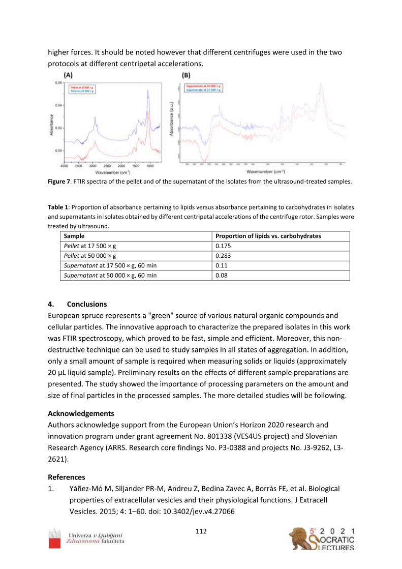
112
higher forces. It should be noted however that different centrifuges were used in the two
protocols at different centripetal accelerations.
Figure 7. FTIR spectra of the pellet and of the supernatant of the isolates from the ultrasound-treated samples.
Table 1: Proportion of absorbance pertaining to lipids versus absorbance pertaining to carbohydrates in isolates
and supernatants in isolates obtained by different centripetal accelerations of the centrifuge rotor. Samples were
treated by ultrasound.
Sample Proportion of lipids vs. carbohydrates
Pellet at 17 500 × g 0.175
Pellet at 50 000 × g 0.283
Supernatant at 17 500 × g, 60 min 0.11
Supernatant at 50 000 × g, 60 min 0.08
4. Conclusions
European spruce represents a "green" source of various natural organic compounds and
cellular particles. The innovative approach to characterize the prepared isolates in this work
was FTIR spectroscopy, which proved to be fast, simple and efficient. Moreover, this non-
destructive technique can be used to study samples in all states of aggregation. In addition,
only a small amount of sample is required when measuring solids or liquids (approximately
20 µL liquid sample). Preliminary results on the effects of different sample preparations are
presented. The study showed the importance of processing parameters on the amount and
size of final particles in the processed samples. The more detailed studies will be following.
Acknowledgements
Authors acknowledge support from the European Union’s Horizon 2020 research and
innovation program under grant agreement No. 801338 (VES4US project) and Slovenian
Research Agency (ARRS. Research core findings No. P3-0388 and projects No. J3-9262, L3-
2621).
References
1. Yañez-Mó M, Siljander PR-M, Andreu Z, Bedina Zavec A, Borràs FE, et al. Biological
properties of extracellular vesicles and their physiological functions. J Extracell
Vesicles. 2015; 4: 1–60. doi: 10.3402/jev.v4.27066

113
2. de Palma M, Ambrosone A, Leone A, del Gaudio P, Ruocco M, et al. Plant roots release
small extracellular vesicles with antifungal activity. Plants. 2020; 9: 1–14.
doi: 10.3390/plants9121777
3. Cui Y, Gao J, He Y, Jiang L, Plant extracellular vesicles. Protoplasma. 2020; 257: 3–12.
doi: 10.1007/s00709-019-01435-6
4. Halperin W, Jensen WA, Ultrastructural changes during growth and embryogenesis in
carrot cell cultures. J. Ultrasructure Res. 1967; 18: 428–443.
doi: 10.1016/S0022-5320(67)80128-X
5. Halperin W, Alternative morphogenetic events in cell suspensions. Am J Bot. 1966;
53(5): 443–453. doi: https://doi.org/10.2307/2440343
6. Zhuang X, Xiang X, Grizzle W, Sun D, Zhang S, et al. Treatment of brain inflammatory
diseases by delivering exosome encapsulated anti-inflammatory drugs from the nasal
region to the brain. Mol Ter. 2011; 19(10): 1769–1779. doi: 10.1038/mt.2011.164
7. Ju S, Mu J, Dokland T, Zhuang X, Wang Q, et al. Grape exosome-like nanoparticles
induce intestinal stem cells and protect mice from DSS-induced colitis. Mol Ther.
2013; 21(7): 1345–1357. doi: 10.1038/mt.2013.64
8. Jeran M, Barrios-Francisco R, Sedušak Kljakič A, Remškar H, Novak U, Non-destructive
characterisation of natural materials: quantitative determination of borneol and
limonene in European spruce needles (Picea abies) by FTIR spectroscopy. In Kralj-Iglic
V, editor. Socratic lectures: 4th International Minisymposium, Ljubljana, Faculty of
Health Sciences, University of Ljubljana (Slovenia). 2021; pp. 79–86. ISBN: 978-961-
7112-02-3
9. Jeran M, Navadna smreka (Picea abies) kot vir aktivnih učinkovin/ Engl. European
spruce (Picea abies) as a source of biologically active compounds. Trdoživ. 2020; 9(2):
22–24. ISSN: 2232-5999. Available from:
https://issuu.com/trdoziv/docs/trdoziv18_web_v01
10. Ebringerova A, Hromadkova Z, An overview on the application of ultrasound in
extraction, separation and purification of plant polysaccharides. Cent Eur J Chem.
2010; 8(2): 243–257. doi: 10.2478/s11532-010-0006-2
11. Naumann D, Infrared Spectroscopy of cells, tissues and body fluids. In Roberts GCK,
editor. Encyclopedia of biophysics, Berlin, Heidelberg: Springer. 2013; pp. 1057–1065.
doi: https://doi.org/10.1007/978-3-642-16712-6_120
12. Božič D, Hočevar M, Kononenko V, Jeran M, Štibler U, et al. Pursuing mechanisms of
extracellular vesicle formation. Effects of sample processing. In Bongiovanni A,
Pocsfalvi G, Manno M, Kralj-Iglič V, editors. Adv. Biomembr. Lipid Self-Assembly. 2020;
32: 113–155. doi: 10.1016/bs.abl.2020.09.003
13. Kralj-Iglič V, Pocsfalvi G, Mesarec L, Šuštar V, Hägerstrand H, Iglič A, Minimizing
isotropic and deviatoric membrane energy – An unifying formation mechanism of
different cellular membrane nanovesicle types. PLoS One. 2020; 15(12): 1–25,
doi: 10.1371/journal.pone.0244796

114

115
__________________
Renin-angiotensin system inhibitors and their implications for COVID-19
treatment
Koren Jerneja1, Scott Derek1, Jeran Marko2,3,* 1School of Medicine, Medical Sciences and Nutrition, University of Aberdeen, Aberdeen, UK 2Laboratory of Clinical Biophysics, Faculty of Health Sciences, University of Ljubljana,
Slovenia 3Laboratory of Physics, Faculty of Electrical Engineering, University of Ljubljana, Slovenia
Abstract
The novel coronavirus, SARS-CoV-2, is responsible for the recent epidemic outbreak and has
raised a lot of concern over the past year. It has so far been identified that the virus enters
the human body via a membrane-bound enzyme called Angiotensin-converting enzyme II
(ACE2), an important part of the Renin-Angiotensin System (RAS). RAS is responsible for
regulating blood pressure and volume and therefore often used as a drug target to treat
hypertension, heart conditions and diabetes. These drugs that can affect the blood pressure
by working on RAS are known as RAS inhibitors. These facts made scientists and clinicians
question, whether taking RAS inhibitors might positively or negatively impact the onset and
progression of COVID-19. This review aims to briefly explain the RAS pathway, its major
elements and roles in human physiology as well as how that is affected by RAS inhibitors. It
also aims to relate that to COVID-19 and outline the possible correlations.
__________________

116
1. Introduction
Severe acute respiratory syndrome coronavirus (SARS-CoV-2) is the novel coronavirus that
has rapidly spread around the globe since its first detection in December 2019, causing a
global pandemic [1, 2]. It is the cause of COVID-19, which is associated with respiratory
problems, fever and, in some cases, inappropriate inflammatory response resulting in mild
to severe lung damage [2, 3]. It enters the body by interacting with the Angiotensin-
Converting Enzyme 2 (ACE2) expressed on the cell surface of different tissues, including the
lungs and kidneys [3-10]. ACE2 is a part of a very important system in our body called the
Renin-Angiotensin system (RAS), which is involved in controlling blood volume and pressure
as well as, to a certain extent, inflammation [1, 9, 11]. Therefore, drugs that inhibit certain
parts of the RAS pathways, collectively known as RAS inhibitors, are often utilised to treat
hypertension in patients with cardiovascular diseases, diabetes and other pathologies, many
of which have recently been associated with potentially higher risk of severe COVID-19 [2, 3,
7, 8, 12]. Since the SARS-CoV-2 and RAS inhibitors share a target pathway, there has been a
concern that the two may interfere, resulting in increased risk of severe infection in patients
taking RAS inhibitors [3, 14]. This review systematically covers the concerning pathways and
the recent implications for RAS inhibitors in COVID-19 treatment.
2. RAS Pathway
The renin-angiotensin system (RAS) involves a cascade of enzymes, particularly proteases,
which ultimately work to regulate the blood pressure and volume as well as, to a certain
extent, inflammation [3, 9, 11, 15]. The whole process (schematically depicted in Figure 1)
starts with production of angiotensinogen in the liver, which then travels to the kidneys,
where it is cleaved by a protease called renin to produce angiotensin I (Ang I) [11]. The next
step in the pathway is cleavage of Ang I to its active form, angiotensin II (Ang II), which is
done by angiotensin-converting enzyme I (ACE), expressed on the surface of cells in the
lungs, kidneys, intestine and other organs [3, 9, 11]. Ang II can then exhibit its effects by
binding to either one of its two receptors – angiotensin II receptor type 1 (AT1R) or type 2
(AT2R). Both are G-protein coupled receptors, but they exhibit opposite effects [10, 11].
AT1R is associated with increased inflammation, mainly through the release of cytokines
including TNF-α and IL-1, water retention as well as constriction of the blood vessels [2, 3, 7,
9, 11]. AT2R, on the other hand, has primarily anti-inflammatory effects coupled with
vasodilation [3, 7, 9, 11]. AT1R and AT2R therefore exhibit antagonistic actions and work to
oppose one another [7]. An alternative Ang II pathway involves a carboxypeptidase called
Angiotensin-converting enzyme II (ACE2), which is the known entry point for SARS-CoV-2
expressed on the surface of certain cells in the lungs, blood vessels and some other specific
tissues [3, 9, 11]. ACE2 cleaves Ang II into Angiotensin-(1-7) (Ang-(1-7)) or Ang I into
Angiotensin-(1-9) (Ang-(1-9)), which is then transformed into Ang-(1-7) by ACE [4, 9, 11, 12].
Ang-(1-7) can then bind to G-protein coupled receptors called Mas receptors to achieve
similar effects than Ang II binding to AT2R – vasodilation, decreased inflammation, primarily
by lowering levels of cytokines like IL-6, and increased renal water secretion [2-4, 9, 10, 11,
16]. ACE2, Ang-(1-7) and Ang-(1-9) show opposing functions to the ACE-Ang II pathway and

117
due to this fact, ACE2 and its pathway are thought to play a protective role against
respiratory infection, lung injury, cardiovascular diseases and diabetes and reduced ACE2
presence can lead to several health issues [2-4, 7, 12, 16, 17].
Figure 4. The two opposing axis of the RAS pathway and the effects of ACE inhibitors and AT1R inhibitors on
different intermediates and enzymes in the pathway. Adapted from [11].
As outlined in this section, ACE and ACE2 have opposing effects, similar to the ones
described in AT1R and AT2R, and can therefore regulate the RAS pathway and its
physiological effects on the body [2, 3, 9, 11]. They form two important opposing axis of the
RAS pathway – the ACE/Ang II/AT1R axis and the ACE2/Ang(1-7)/Mas axis [3, 4, 9, 11]. They
have to be kept in strict balance as interruptions in regulation of these two pathways are
critical in cardiovascular diseases and hypertension [3, 9, 15, 18].
3. RAS inhibitors
There are different pharmacological substances, collectively known as RAS inhibitors, that
can interfere with specific steps in the RAS pathway to prevent increased blood pressure and
vasoconstriction [5]. These include, but are not limited to, angiotensin-converting enzyme I
(ACE) inhibitors and angiotensin II receptor type 1 blockers (ARB), which block AT1R [2, 5,
11]. They are administered to patients with increased blood pressure and different
cardiovascular problems [2]. ACE inhibitors are mainly involved in preventing ACE from
cleaving Ang I into Ang II and include clinically approved drugs like captopril and enalapril [4,
12]. Although they act via a different pathway than ACE2, it has been indicated that they can
cause upregulation of ACE2 expression as well, but only very moderate evidence is available
up to date [4, 9]. That indicates they could potentially be effective in different lung
conditions by maintaining the ACE/ACE2 ratio and therefore preserving the protective
functions of ACE2 [4]. ARBs, on the other hand, mainly inhibit AT1R and include drugs like

118
losartan and olmesartan [4, 11]. They have known anti-inflammatory abilities and
experiments on animal models showed that they can act to upregulate ACE2 expression as
well and this association seems to be more supported by evidence than the one regarding
ACE [4]. However, neither of the two mentioned RAS inhibitors interacts with ACE2 directly
[1].
4. RAS inhibitors and COVID-19
As outlined in section 2, angiotensin converting enzyme 2 (ACE2) has a role diagonally
opposite to ACE, the enzyme that ACE inhibitors act on. Through the downstream signalling
pathways, it can cause dilation of the blood vessels and consequently, a decrease in blood
pressure [16, 19]. ACE2 serves as the entry point for SARS-CoV-2 through the binding of the
viral spike proteins (S proteins), particularly the S1 subunit, with the enzyme on the cell
surface [2, 3, 4, 6, 9, 17, 19]. For the virus to successfully enter the cell, another membrane
enzyme called transmembrane protease, serin 2 (TMPRSS2) has to be present alongside
ACE2 as well [2, 12].
Studies done indicate that binding and entry of the SARS-CoV-2 lowers the presence of ACE2
on the cell surface through endocytosis of the bound virus as well as potentially targeted
downregulation of the enzyme expression, primarily by increasing metallopeptidase domain-
containing protein 17 (ADAM-17) expression [1, 2, 7, 9, 17]. ADAM-17 can then cleave of the
membrane-bound ACE2 and cause further repression of ACE2 expression, which was shown
in murine animal models [1, 2, 7, 15]. That means that the ACE1/ACE2 balance and therefore
the protective effects of the ACE2/Ang(1-7)/Mas pathway in respiratory conditions are lost
and Ang II starts accumulating leading to its increased action [2, 4, 10, 11]. It has been
proposed that administering synthetic Ang-(1-7) and Mas and AT2R agonists could
counterbalance that and therefore help in lung injury, which often presents in COVID-19
patients [10, 11]. However, the details of the signalling pathways associated with Mas
receptors are still not well understood so further preclinical and research data is required to
support the implications [10]. Another proposed novel therapeutic approach currently still
being researched is synthetic ACE2 that could be administered to COVID-19 infected patients
to reinforce the appropriate ACE/ACE2 balance [10].
Another concerning consequence of the ACE2 downregulation that offers another possible
treatment target, are high levels of Ang II, which play an important role in lung damage and
have been detected in patients with COVID-19 [2, 8, 9, 10, 17]. Ang II induces
vasoconstriction, which can lead to lower blood flow in the lungs, interrupting the gas
exchange. Additionally Ang II can also increase infiltration of immune cells and damage to
the blood vessels [2]. It has also been implicated that Ang II can act to stimulate ADAM-17
activity when it binds to AT1R [17]. In fact, higher levels of Ang II have been associated with
the onset of acute respiratory distress syndrome (ARDS), a frequent and very serious
manifestation of COVID-19 [2, 16, 18]. Based on those facts, it was suggested that using ACE
inhibitors and ARBs could potentially be beneficial as they could reduce lung damage in
COVID-19 patients by preventing the increased Ang II levels from having an effect [2, 10, 11,
18]. Although both ACE inhibitors and ARBs are well established and safe drugs, the different

119
pathways they use to achieve the results offer different possibilities as well possible
disadvantages [10].
ARBs, specifically AT1R inhibitors would prevent the Ang II from binding to AT1R and
therefore facilitate its binding to AT2R [11]. As outlined, that would result in a downstream
anti-inflammatory response and therefore exhibit protective functions – however, these
signalling pathways are still not well understood so further data must be provided to confirm
these effects [11, 18]. In addition, Ang II, not able to bind its receptor, would start to
accumulate and therefore form a pool of substrate for ACE2 [18]. ACE inhibitors, on the
other hand, inhibit Ang II formation and prevent the body from using Ang-(1-7) to form Ang-
(1-5), meaning that more of it would be preserved to bind to Mas receptors. ACE inhibitors
therefore lead to higher levels of Ang-(1-7) and decreased Ang II, which indicates that they
could have beneficial effects for COVID-19 patients [1, 11]. However, one problem
associated with this proposal is that ACE inhibitors can cause potential side effects that
include coughing, which could affect the progression of COVID-19 as a respiratory disease
[10]. However, whether these implications are clinically significant in terms of COVID-19
treatment is yet to be proven with consistent scientific clinical research [10, 11]. It is known
that there are many other factors that affect the progression of COVID-19 and even if RAS
inhibitors did prove to be efficient, detailed clinical data would have to be collected to
determine any unwanted side effects as well as the correct dose and timing of
administration [10, 11].
The points discussed mostly mention using RAS inhibitors as a treatment options in
diagnosed COVID-19 patients. However, the major concern associated with RAS inhibitors is
that they could potentially lead to higher risk of infection with SARS-CoV-2 for those taking
them [18]. That was postulated based on the implication that AT1R and ACE inhibitors might
cause an increase in ACE2 expression, which could facilitate SARS-CoV-2 entry into the cells
[3, 5, 9, 10, 20]. That is, of course, not beneficial for patients with pre-existing health
conditions such as hypertension and cardiovascular diseases [9, 20]. These effects have been
implicated mostly in ARBs, while limited data is available for ACE inhibitors [12, 18].
However, even in ARBs most evidence for these implications comes from animal studies,
where higher doses of ACE and AT1R inhibitors are often utilised [20]. In fact, most human
studies found no correlation between RAS inhibitors and increased ACE2 expression and
clinical data does not show any strong support for a higher risk of SARS-CoV infection
associated with ARBs or ACE inhibitors [10, 18, 20, 21].
Despite this contradicting evidence, much of which still needs further evaluation, it is still
hard to say, whether RAS inhibitors significantly affect the progression of COVID-19 or
increase the chances of infection for the patients taking them [3, 9]. However, it is important
to note that RAS inhibitors provide other major health benefits for the patients taking them
and strong scientific evidence proving the correlation between these drugs and an increased
risk of severe COVID-19 infection would have to be provided to outweigh the benefit [5, 9,
19]. Therefore, most scientific data advises continuing administration of RAS inhibitors until
or unless further clinical data supporting the negative correlation is provided [3, 20].

120
5. Clinical results
Consistent clinical research in this area is difficult to carry out in larger groups that would
allow statistically significant results and conclusions to be made. As outlined in the report,
there are implications for both negative and positive effects of RAS inhibitors on COVID-19
progression and infection [2]. Since the onset of the COVID-19 pandemic, several clinical
studies have been carried out to establish the link between RAS inhibitors and COVID-19 [2].
One of them was a retrospective study that included 126 patients with diagnosed
hypertension done in 2020 in Wuhan, China by Yang et al [22]. It included 126 patients, 43 of
them received either ARBs or ACE inhibitors and 83 of them received other medication [22].
Scientists found no correlation between ACE inhibitors and ARBs an increased risk of COVID-
19 infection [22]. It was observed that patients taking ACE inhibitors or ARBs actually had a
lower risk of severe infection as well as mortality rate, but these results were not statistically
significant (p = 0.061 and p = 0.216 respectively) [22]. A similar, but larger-scale study was
done on a national level in South Korea in 2020 by Jung et al. [23]. In this case, 5179 patients
were studied, of which 762 used RAS inhibitors, while the remaining 4417 did not [23]. The
results showed that RAS inhibitors did not independently statistically significantly affect the
mortality (p = 0.60) or the severity of the diseases [23]. Similar results were obtained by Lam
et al., who studied 614 patients with diagnosed hypertension that were hospitalised due to
COVID-19 [24]. The main aim of this study was to assess, whether it is more beneficial to
stop ACE inhibitor/ARBs therapy or continue with normal administration of these drugs [24].
279 of these patients did not take ACE inhibitors or ARBs (control), 171 patients stopped
using ACE inhibitors or ARBs upon hospitalisation and 164 patients followed their normal
ACE inhibitor/ARB therapy [24]. The results showed that continuous usage of ACE inhibitors
or ARBs statistically significantly lowered the mortality rate compared to terminated usage
of these drugs (p = 0.001) [24]. However, some other reported studies found no correlation
between RAS inhibitors and COVID-19 [8, 25]. This shows that the results are still lacking
consistency and more large-scale trials are needed to provide more accurate results – until
then, such data should be treated carefully [2, 18]. Several trials are currently in progress or
recruiting and more data is expected soon.
6. Conclusion
COVID-19 occurs as a consequence of an infection with the novel coronavirus, SARS-CoV-2
[26]. As outlined in the report, there are implications for both advantageous and harmful
effects of ARBs and ACE inhibitors on the infection or progression of COVID-19 [10]. It is
indicated that RAS inhibitors could stimulate expression of ACE2, which could facilitate SARS-
CoV-2 infection, but their role in limiting the damaging effects of elevated Ang II could
prevent some very serious conditions associated with COVID-19 [2, 17]. Clinical data
suggests that there is currently no strong scientific proof that ACE inhibitors or ARBs carry a
higher risk for severe COVID-19 and should therefore continue to be administered to the

121
appropriate patients [21]. Further research in preclinical and clinical trials are required to
assess those implications and form any conclusions that could affect the patients.
Acknowledgements
Authors acknowledge support from the European Union’s Horizon 2020 research and
innovation program under grant agreement No. 801338 (VES4US project) and Slovenian
Research Agency (ARRS. Research core fundings No. P3-0388 and projects No. J3-9262, L3-
2621).
References
1. Brojakowska A, Narula J, Shimony R, Bander J. Clinical Implications of SARS-CoV-
2 Interaction With Renin Angiotensin System. J Am Coll Cardiol. 2020; 75: 3085-3095.
doi: 10.1016/j.jacc.2020.04.028
2. Wang J, Edin M, Zeldin D, Li C, Wang D, Chen C. Good or bad: Application of RAAS
inhibitors in COVID-19 patients with cardiovascular comorbidities. Pharmacol Ther.
2020; 215: 107628. doi: 10.1016/j.pharmthera.2020.107628
3. Parit R, Jayavel S. Association of ACE inhibitors and angiotensin type II blockers with
ACE2 overexpression in COVID-19 comorbidities: A pathway-based analytical study. Eur
J Pharmacol. 2021; 896: 173899. doi: 10.1016/j.ejphar.2021.173899
4. Chatterjee B, Thakur S. ACE2 as a potential therapeutic target for pandemic COVID-
19. RSC Adv. 2020; 10: 39808-39813. doi: 10.1039/D0RA08228G
5. Haroon S, Subramanian A, Cooper J, et al. Renin-angiotensin system inhibitors and
susceptibility to COVID-19 in patients with hypertension: a propensity score-matched
cohort study in primary care. BMC Infect Dis. 2021; 21.
doi: 10.1186/s12879-021-05951-w
6. Kralj Iglič V, Dahmane R, Griessler Bulc T, et al. From Extracellular Vesicles to Global
Environment: A Cosmopolite Sars-Cov-2 Virus. 2020; IJCMCR, 4.
doi: 0.46998/IJCMCR.2020.04.000079
7. Santos RAS, Oudit GY, Verano-Braga T, Canta G, Steckelings UM, Bader M. The renin-
angiotensin system: going beyond the classical paradigms. Am J Physiol Heart Circ
Physiol. 2019; 316: H958-H970. doi: 10.1152/ajpheart.00723.2018
8. Shukla A, Banerjee M. Angiotensin-Converting-Enzyme 2 and Renin-Angiotensin
System Inhibitors in COVID-19: An Update. High Blood Press Cardiovasc Prev. 2021; 28:
129-139. doi: 10.1007/s40292-021-00439-9
9. South AM, Brady TM, Flynn JT. ACE2 (Angiotensin-Converting Enzyme 2), COVID-19,
and ACE inhibitor and Ang II (Angiotensin II) receptor blocker use during the pandemic.
Hypertension. 2020; 76: 16-22. doi: 10.1161/HYPERTENSIONAHA.120.15291
10. Sriram K, Loomba R, Insel P. Targeting the renin−angiotensin signaling pathway in
COVID-19: Unanswered questions, opportunities, and challenges. Proc Natl Acad Sci
USA. 2020; 117: 29274-29282. doi: 10.1073/pnas.2009875117

122
11. D’Ardes D, Boccatonda A, Rossi I, et al. COVID-19 and RAS: Unravelling an Unclear
Relationship. Int J Mol Sci. 2020; 21: 3003. doi: 10.3390/ijms21083003
12. Danser A, Epstein M, Batlle D. Renin-Angiotensin System Blockers and the COVID-19
Pandemic. Hypertension. 2020; 75: 1382-1385.
doi: 10.1161/HYPERTENSIONAHA.120.15082
13. Sharma S. COVID-19: A Concern for Cardiovascular Disease Patients. Cardiovasc
Toxicol. 2020, 20: 443-447. doi: 10.1007/s12012-020-09596-0
14. Wysocki J, Lores E, Ye M, Soler M, Batlle D. Kidney and Lung ACE2 Expression after an
ACE Inhibitor or an Ang II Receptor Blocker: Implications for COVID-19. J Am Soc
Nephrol. 2020; 31: 1941-1943. doi: 10.1681/ASN.2020050667
13. Patel VB, Zhong JC, Grant MB, Oudit GY. Role of the ACE2/Angiotensin 1–7 Axis of the
Renin–Angiotensin System in Heart Failure. Circ Res. 2016; 118: 1313-1326. doi:
10.1161/CIRCRESAHA.116.307708
14. Santos RAS, Sampaio WO, Alzamora AC, Snatos DM, Alenina N, et al. The
ACE2/Angiotensin-(1–7)/MAS Axis of the Renin-Angiotensin System: Focus on
Angiotensin-(1–7). Physiol Rev. 2018; 98: 505-553.
doi: 10.1152/physrev.00023.2016
15. Gheblawi M, Wang K, Viveiros A, et al. Angiotensin-Converting Enzyme 2: SARS-CoV-2
Receptor and Regulator of the Renin-Angiotensin System. Circ Res. 2020; 2020: 1456–
1474. doi: 10.1161/CIRCRESAHA.120.317015
16. Sarzani R, Giulietti F, Di Pentima C, Giordano P, Spannella F. Disequilibrium between
the classic renin-angiotensin system and its opposing arm in SARS-CoV-2-related lung
injury. Am J Physiol Lung Cell Mol Physiol. 2020; 319: L325-L336.
doi: 10.1152/ajplung.00189.2020
17. Patoulias D, Katsimardou A, Stavropoulos K, Imprialos K, Kalogirou M, Doumas M.
Renin-Angiotensin System Inhibitors and COVID-19: a Systematic Review and Meta
Analysis. Evidence for Significant Geographical Disparities. Curr Hypertens Rep. 2020;
22(11):90. doi: 10.1007/s11906-020-01101-w
18. Sriram K, Insel P. Risks of ACE Inhibitor and ARB Usage in COVID‐19: Evaluating the
Evidence. Clin Pharmacol Ther. 2020; 108: 236-241. doi: 10.1002/cpt.1863
19. Mackey K, Kansagara D, Vela K. Update Alert 7: Risks and Impact of Angiotensin-
Converting Enzyme Inhibitors or Angiotensin-Receptor Blockers on SARS-CoV-2
Infection in Adults. Ann Intern Med. 2021; 174: W25-W29. doi: 10.7326/L20-1446
20. Yang G, Tan Z, Zhou L, et al. Effects of Angiotensin II Receptor Blockers and ACE
(Angiotensin-Converting Enzyme) Inhibitors on Virus Infection, Inflammatory Status,
and Clinical Outcomes in Patients With COVID-19 and Hypertension. Hypertension.
2020; 76: 51-58. doi: 10.1161/HYPERTENSIONAHA.120.15143
21. Jung SY, Choi JC, You SH, Kim WY. Association of Renin-angiotensin-aldosterone
System Inhibitors With Coronavirus Disease 2019 (COVID-19)- Related Outcomes in
Korea: A Nationwide Population-based Cohort Study. Clin Infect Dis. 2020; 71: 2121-
2128. doi: 10.1093/cid/ciaa624

123
22. Lam KW, Chow KW, Vo J,Hou W, Li H, et al. Continued In-Hospital Angiotensin-
Converting Enzyme Inhibitor and Angiotensin II Receptor Blocker Use in Hypertensive
COVID-19 Patients Is Associated With Positive Clinical Outcome. J Infect Dis. 2020;
222: 1256-1264. doi: 10.1093/infdis/jiaa447
23. Mancia G, Rea F, Ludergnani M, Apolone G, Corrao G. Renin–Angiotensin–Aldosterone
System Blockers and the Risk of Covid-19. N Engl J Med. 2020; 382: 2431-2440.
doi: 10.1056/NEJMoa2006923
24. Choate J, Aguilar-Roca N, Beckett E, et al. International Educators’ Attitudes,
Experiences, and Recommendations After an Aabrupt Transition to Remote Physiology
Laboratories. Adv Physiol Educ. 2021; 45: 310-321. doi: 10.1152/advan.00241.2020

124

125
___________________
Study of the cannabinoid profile and microbiological activity of industrial hemp
(Cannabis Sativa subsp. Sativa L.)
Pečan Luka Irenej1, Štukelj Roman2,*, Torkar Godič Karmen3, Jeran Marko2,4,*
1University of Ljubljana, Biotechnical faculty, Department of Biotechnology, Ljubljana,
Slovenia 2University of Ljubljana, Faculty of Health Sciences, Laboratory of Clinical Biophysics,
Ljubljana, Slovenia 3University of Ljubljana, Faculty of Health Sciences, 3Department of Sanitary Engineering,
Ljubljana, Slovenia 4University of Ljubljana, Faculty of Electrical Engineering, Laboratoy of Physics, Ljubljana,
Slovenia
Abstract
The main motive of this research is to study cannabis for therapeutic and clinical usage. For
this purpose, chemical and microbiological analysis of ten cannabis samples for industrial
usage were studied. In the chemical part, the content of cannabinoids in the dried buds of
hemp from two different growing seasons were characterized by high performance liquid
chromatography (HPLC). We found that only the variety Futura-75 had a total concentration
of cannabidiol within the variety specification (1.50–2.00%), while the concentrations of
cannabidiol in the remaining nine varieties from both seasons were below the lower limit of
the specification for each variety. The measured Δ-9-tetrahydrocannabinol contents ranged
from 0.01% in the Uso-31 variety to 0.63% in the Antal variety. All samples had a total % Δ-9-
tetrahydrocannabinol below the permissible limit of 0.20%, except for the Tizsa and Antal
varieties. We also examined the microbiological quality of these samples after storage,
following the guidelines for the microbiological safety of food. The analysis determined the
presence of microorganisms in the samples that could be pathogenic at higher
concentrations for the end consumer when used for the preparation of herbal infusions. The
microbiological quality of all tested samples corresponded to the normatives according to
national legislation. We found differences in microbiological quality between individual
varieties, which were otherwise grown in identical growing conditions and later treated
equally in all phases of storage. The analysed material was both microbiologically and
chemically safe for use for human consumption.
___________________

126
1. Objective and purpose
The main goal of the research was to determine the chemical and microbiological profile of
ten varieties of cannabis, to find out the concentration of phytocannabinoids in each variety
and to check how the concentration of the same variety changes in two different growing
seasons.
The purpose of the research was to check the microbiological quality of dried cannabis
samples after the storage phase and determine how the quality itself is affected by growth
and storage factors. In order to determine the safety of every single sample that could be
used as food, we also determined the presence of mycotoxins (or more precisely aflatoxins)
in individual samples of dried cannabis.
2. Introduction
Cannabis (Cannabis sativa), commonly known as marijuana, has been used by mankind since
ancient times. From more than a millennium BC to the end of the 19th century, it was among
the most important agricultural crops and industrial raw material. The vast majority of fibres
and fabrics, light oil, paper, incense and medicines were made from hemp. Cannabis acts as
a stimulant, depressant (antipsychotic) and a hallucinogen. Its main psychoactive ingredient
is tetrahydrocannabinol (THC); it also contains more than 80 cannabinoids. Today it is used
for recreational, medical, nutritional and industrial purposes.
In 2019, important legal steps were taken for the “rehabilitation” of cannabis and its
decriminalization at the level of the European Union since the European Parliament
approved a Resolution on the use of cannabis for medical purposes with the aim of
encouraging governments’ support for research and the availability of medical cannabis in
EU countries. In the same year on December, a meeting of the Commission on Narcotic
Drugs was held in Vienna, attended by all EU Member States and signatories of the 1961
Convention on Narcotic Drugs and placed Cannabis in a group of predominantly harmless
substances. Tetrahydrocannabinol (THC) was also included in this group, and cannabidiol
(CBD) was excluded from the system of international surveillance, as no harm to health can
be demonstrated [1].
3. Hemp
a. Cannabis Cannabis is a genus of flowering plants from the family Cannabaceae. It is found in all
latitudes, as it is phenotypically very adaptable to environmental factors. Cannabis is an
annual, dioecious, flowering herb. The leaves are palmately compound or digitate with serrate
leaflets. The first pair of leaves usually have a single leaflet, the number gradually increases up
to a maximum of about thirteen leaflets per leaf (usually seven or nine), depending on the
variety and growing conditions. Cannabis has been described as having one of the most
complicated mechanisms of sex determination among the dioecious plants [2].

127
b. Biologically active compounds in hemp Nowadays hemp is one of the most chemically researched plants along with more than 420
known compounds. The most interesting ingredients are found in the secretion glands called
trichomes, which are distributed over the surface of hemp plant. Although trichomes are
found distributed over the entire surface of both male and female plants, they are especially
concentrated in some parts of the female inflorescence. The resin secreted by trichomes
contains various ingredients, among which cannabinoids, terpenes and flavonoids are the
important ones which are secondary metabolism products [1].
Cannabinoids are the main biologically active components of cannabis. Literature reports
over 90 different cannabinoids that have been detected until today, although some of them
are degradation products. Cannabinoids are, in a broader sense, substances that bind to
cannabinoid receptors and cause certain effect through this binding [3].
c. Δ-9-Tetrahydrocannabinol (THC) THC is a glassy solid, soluble in alcohols, hydrocarbons and oils but insoluble in water. The
boiling point of THC is 165 °C, which is the lowest required heating temperature when
administered by inhalation. As a narcotic, it is classified in the second group of illicit drugs, so
it is allowed for medical and research purposes. THC is an active substance authorized by the
US Food and Drug Administration and the European Medicines Agency, as it is used in
authorized medicines such as Marinol®, CesametTM and Sativex® [4].
The actions of THC result from its partial agonist activity at the cannabinoid receptor CB1 (Ki
= 10 nM), located mainly in the central nervous system, and the CB2 receptor (Ki = 24 nM),
mainly expressed in cells of the immune system. The psychoactive effects of THC are
primarily mediated by the activation of cannabinoid receptors which result in a decrease in
the concentration of the second messenger molecule cAMP through inhibition of adenylate
cyclase. The presence of these specialized cannabinoid receptors in the brain led researchers
to the discovery of endocannabinoids, such as anandamide and 2-arachidonoyl glyceride (2-
AG) [5].
THC is a lipophilic molecule which may bind non-specifically to a variety of entities in the
brain and body, such as adipose tissue (fat). THC, as well as other cannabinoids that contain
a phenol group, possess mild antioxidant activity sufficient to protect neurons against
oxidative stress, such as that produced by glutamate-induced excitotoxicity [6].
d. Cannabidiol (CBD) Cannabidiol (CBD) was first isolated from cannabis in 1940, and its structure was discovered
in 1963. Numerous synthetic extraction processes are known, and it is semi-synthetically
derived from limonene. At room temperature it is a colourless, white to yellow crystalline
solid boiling at 175 °C. In the presence of certain acids or high temperature during pyrolysis,
smoking can cyclize it to THC, but in very small amounts. CBD is a very popular raw material
in dietary supplements and cosmetics. Cannabidiol is a phytocannabinoid derived from the
cannabis type and has analgesic, anti-inflammatory, antineoplastic and chemo preventive
effects but no psychoactive action. CBD stimulates endoplasmic reticulum (ER) stress and

128
inhibits AKT/mTOR signalling, thereby activating autophagy and promoting apoptosis. CBD
also increases the production of reactive oxygen species (ROS), which further increases
apoptosis. This agent also regulates the expression of intercellular adhesion molecule 1
(ICAM-1) and tissue matrix metalloproteinase-1 (TIMP1) inhibitors and reduces the
expression of DNA 1 binding inhibitor (ID-1). This inhibits the invasiveness and metastasis of
cancer cells. CBD can also activate the transient receptor potential of vanilloid type 2
(TRPV2) which may increase the uptake of various cytotoxic agents into cancer cells. The
analgesic effect of CBD is mediated through its binding to CB1 receptors [7].
4. Hypotheses
a. Quantitative determination of cannabinoid concentration Hypothesis 1: In cannabis varieties for the purpose of cultivation for stems, the content of
cannabidiol (CBD) and other cannabinoids (THC, CBG, CBD, THC) will be detected by HPLC
analysis and cannabis buds at full maturity will be useful for further processing in terms of
cannabinoid content and concentration.
Hypothesis 2: Weather conditions in two seasons (2017 and 2018), harvesting time and the
entire growing season will significantly affect the presence and concentration of
cannabinoids in the same varieties. In plants with a shorter growth time, the concentration
of cannabinoids will be lower.
b. Microbiological quality of samples Hypothesis 3: In samples representing different varieties of cannabis, the number and the
presence of individual species of microorganisms will be different. These differences will be
due to weather and the specificity of each cannabis variety.
Hypothesis 4: The presence of microorganisms in cannabis samples will be under the limits
of the normative specified in the Guidelines for microbiological safety of food intended for
the final consumer.
c. Mycotoxins Hypothesis 5: In the samples in which microbiological analyses will show a higher presence
of mould and yeast, higher presence of mycotoxins will also be detected.
5. Experimental
a. Method of drying hemp samples After collecting the plant samples, they were dried in the same way under the same
conditions. The samples were dried in an oven as drying under direct sunlight affects
oxidative processes and cannabinoid degradation. In both years, the harvested plant parts
were tied into a bundle of 15 together; drying in the kiln began immediately. The bundles
were dried for 50 hours at 40 °C.
b. Samples Ten different cannabis varieties were used for the samples, namely four monoecious (Fedora
17, Santhica 27, Futura 75 and Uso 31) and six dioecious varieties (KC Dora, Kompolti hybrid
TC, Monoica, Tisza, Tiborszallasi, and Antal). All samples were obtained in 2017 in the

129
laboratory field of the Biotechnical Faculty at University of Ljubljana, where a varietal
experiment of hemp production for stem purposes was performed.
c. Preparation of the general suspension for microbiological analysis The bags in which the samples were stored were first shaken to ensure that cannabis leaves
are well mixed. They were then disinfected with 70% ethanol and aseptically opened near
the burner. Using a sterile spoon, 10.0 g of the sample was transferred to sterile bags, which
were placed in a larger beaker for easier work. 90.0 mL of sterile 2% potassium
dihydrogenphosphate was added to the bags, sealed tightly and kneaded in a kneader.
d. Determination of the number of microorganisms in the samples We used the method of colony counting on solid media after decimal dilution of the sample
to determine the number of selected groups of microorganisms using selective media
according the international standards. The number of aerobic mesophilic microorganisms
(aerobic colony count) [8], the number of Enterobacteriaceae including E. coli [9], yeasts and
moulds [10] and endospores of the genus Bacillus were determined in samples, using
standard colony count method [11]. The presence of Salmonella was also detected in 25 g of
each sample [12].
Results were expressed in number of colony forming units (CFU) per gram of sample.
e. Chromatographic analysis for the determination of cannabinoids Cannabinoids were determined using an 1100 Series Agilent Technologies liquid
chromatograph, under the conditions shown in table below. Prior to analysis, the entire
system was rinsed with the mobile phase for half an hour. The labelled vials were stacked in
order on an HPLC apparatus. First, vials with prepared standard solutions were inserted, the
results of which were used to construct a calibration curve. Other sample vials followed.
Using the program, we then determined the areas under the chromatographic peaks from
the obtained chromatograms, and using the calibration curve, we determined the
concentration of cannabinoids in the dried cannabis tops.
Table 1: Conditions for chromatography separation.
f. Preparation of samples for the determination of cannabinoid concentrations Sheaves of individual varieties were shredded and homogenized in a coffee grinder.
Weighing approximately between 500–510 mg of the homogenized sample (in 2 batches)
into a 50 mL Falcon tube and added 10.0 mL of solvent (MeOH/CHCl3, 9:1).
Column Supelco Ascentis® Express 5 μm, C18
(5 μm, 150 mm × 4.6 mm)
Mobile phase Methanol : 1% acetic acid (65:35)
Mobile phase flow 1 mL/min
Injection volume 20 μL
Column temperature 30 °C
Pressure 105 bar
Analysis time 26 minutes

130
The sample was placed in an ultrasonic bath for 15 min. 1.0 mL of the thus prepared sample
was diluted twice in the same volume of mobile phase and it was filtered via syringe into
vials.
g. Preparation of samples for the determination of mycotoxins We put 10.0 g of the dried plant sample into a conical flask and added 150.0 mL of 10% NaCl
solution. The sample was homogenized in an ultrasonic bath for 15 minutes at 25 °C. The
contents were filtered into a beaker and from there 20.0 mL of the filtrate was pipetted into
a flask. 20.0 mL of the filtrate was transferred to 50.0 mL of a mixture of distilled water and
methanol in a ratio (85:15, v/v) and stirred in an ultrasonic bath for 15 minutes. After that,
50.0 mL of dichloromethane was added and shaken for 30 min. The phases were separated
in a separatory funnel by collecting dichloromethane at the bottom of the separating funnel
in a 200 mL conical flask. The contents were dried over water-binding sodium sulphate,
which was filtered after 45 minutes. The dichloromethane phase was evaporated on a miVac
Quattro rotary evaporator and the residue dried to dryness. The dry extract was dissolved in
1.0 mL of methanol and filtered into vials by syringe through a cellulose-acetate filter.
6. Results and Discussion
a. Microbiological quality of samples The purpose of microbiological examinations was to determine the microbiological safety of
individual leaf samples of different varieties of hemp grown in the 2017 season, after two
years of storage in a closed dark place with an average temperature of 20.5 °C and relative
humidity (39%). Microbiological quality was checked according to the Guidelines for
microbiological food safety, which are intended for the final consumer [13]. The results
showed that all samples contained different amounts of microorganisms (Table 2), which is
most likely due to the design and characteristics of each of the variety and its resistance to
pathogens. Samples were stored in food storage bags with a closure system and
appropriately labelled. Samples of dried cannabis leaves could be used as herbal infusions,
so we used guidelines to determine the permitted limit values of individual microorganisms
for tea, coffee and similar products to determine microbiological quality. As can be seen
from the standards in Table 3, none of the samples exceeds the permitted limit values,
which indicates good manufacturing practice, appropriate hygiene standards and
appropriate storage. All tested samples corresponded to the normative according national
legislation. In addition to the groups of microorganisms defined in our legislation, we also
determined the presence of Bacillus species, because they represent a part of cannabis
bacterial microbiome, but can also be pathogen to humans [14].The results showed (Table 2)
that all samples contained different amounts of microorganisms, which is most likely due to
the design and characteristics of each of the variety and its resistance to pathogens. Some
studies used the bioprospecting rationale that hemp and marijuana contain medicinal
compounds that might also harbour competent microbial endophytes capable of providing
health benefits to the host plant and inhibit the growth of pathogen fungi and bacteria [14].

131
The most common endophytes harboured in buds and leaves of Cannabis sativa belong to
the genuses Bacillus, Pseudomonas and Pantoea [15].
It can be concluded that the microbiological quality depends mainly on the individual variety
and its resistance and adaptability to growing conditions, but in any case, there could be
contamination of the sample during treatment. This factor cannot be ruled out as a possible
source of plant contaminants, as soil quality, soil moisture, soil microbial flora, humidity, air
temperature and the number of sunny and rainy days significantly affect plant health and
consequently the presence of microorganisms.
Table 2: Number of individual microorganisms (MO) in CFU/g.
Variety
Total number of microorganisms (log10CFU)
Yeasts and moulds (log10CFU)
Enterobacteria (log10CFU)
Bacillus vegetative forms (log10CFU)
Bacillus endospores (log10CFU)
Santhica 27 4.518514 3.30103 2.633468 1.60206 2.041393
Fedora 17 3 3.30103 2.653213 1.477121 1.30103
Antal 3.908485 3 3.267172 1.477121 1.30103
Uso 31 5.322219 3.69897 3.478566 2,146128 0.69897
Tibor 4 3 3.176091 1.69897 1.477121
KC Dora 4.176091 3 2.579784 1.30103 1.60206
Tisza 4.544068 3 3.294466 1.954243 1.60206
Kompolti
Hybrid TC
4.544068 3 2.662758 1.812913 1
Monoica 4.886491 3.30103 3.482874 1.477121 1.60206
Futura 75 3 3 2.518514 1.30103 0.69897

132
Table 3: Type of microorganism and quality criterion [13].
b. Quantitative determination of cannabinoid concentration When determining the concentrations of total cannabinoids for 2017, the highest value for
total CBD was 15.9 mg/g for the variety Futura 75, and the lowest 2.1 mg/g for the variety
Santhica 27. Only the Futura 75 variety had a total cannabidiol (CBD) value within the
specification limits, while the other nine varieties were below the expected lower limit
(specification in Table 6). The measured THC values ranged for the highest measured in the
Antal variety, namely 3.6 mg/g and the lowest 0.3 mg/g in the Fututra 75 variety. It can be
concluded that all varieties have a total THC below the permissible limit, which is 0.2%,
except for the Tisza and Antal varieties (Table 4).
When determining the concentrations of total cannabinoids for 2018, the highest value for
total CBD was 1.18 mg/g in the variety KC Dora, and the lowest 0.28 mg/g in the variety Uso
31. In the latter, the cannabinoid cannabidiol is the most pronounced, so it is the result is
also expected and in line with the references. All ten varieties were below the expected
lower limit (Table 5). The measured THC values ranged for the highest measured in the
variety Antal, namely 0.6 mg/g and the lowest 0.01 mg/g in the variety Uso 31. It can be
established that all varieties have a total THC below the permissible limit, which is 0.2%,
except for the Antal variety (Table 5 and 6). As can be seen from the graphs and tables, the
concentration of cannabinoids in the same varieties is different in two years, namely in most
varieties lower in 2018 than in 2017, except for the varieties Antal and KC Dora. The main
reason is most likely the earlier collection of cannabis samples (26 days in 2018 compared to
2017), which also meant a shorter vegetation cycle and cessation of growth during the
period when the plant produces the most cannabinoids.
Cannabinoid content is more influenced by factors during plant growth, such as soil
composition, fertilization, soil moisture and weather conditions, with precipitation, air
temperatures and solar radiation, so the growing season also affects cannabinoid
concentration. The current results suggest a possible negative relationship between
cannabinoid concentration and the microorganisms studied.
Type of microorganism Quality criterion
Salmonella spp. n. n. in 25 g (c = 0)
Escherichia coli m = 103 cfu/gM = 104 cfu/g (c = 2)
Molds and Yeasts m = 105 cfu/g, M = 106 cfu/g (c = 1)
Aerobic mesophilic bacteria m = 107 cfu/gM = 108 cfu/g (c = 2)
Enterobacteriaceae m = 10 cfu/gM = 102 cfu/g (c = 1)

133
Table 4: Shows the weight (m) and average values of two measurements of cannabinoids (wt%) with the
corresponding standard deviations (SD) for cannabis varieties for industrial use from 2017. The average total
values of Δ-9-THC and CBD calculated by the equation (THC total = Δ-9-THC-a × 0.877) + Δ-9-THC are also
shown; (CBD total = CBD × 0.877) + CBD. PMD = below the detection limit. wt% 0.1 = 10 mg.
Variety Weight
(mg ± SD)
CBD-a
(wt% ± SD)
CBG
(wt% ± SD)
CBD
(wt% ± SD)
Δ-9-THC
(wt% ± SD)
Δ-9-THC-a
(wt% ± SD)
Sum CBD
(wt% ± SD )
Sum THC
(wt% ± SD)
Monoica 500.4 ± 0.28 1.00 ± 0.02 0.01 0.14 ± 0.01 0.04 0.14 1.02 ± 0.02 0.16
Tibor
Szallasi 500.6 ± 0.42 1.18 ± 0.10 0.01 0.21 ± 0.02 0.05 0.13 ± 0.01 1.24 ± 0.11 0.17 ± 0.02
Tisza 500.8 ± 0.07 1.16 ± 0.05 0.01 0.23 ± 0.02 0.10 ± 0.01 0.20 ± 0.01 1.25 ± 0.07 0.27 ± 0.02
Fedora 17 500.3 ± 0.35 1.26 ± 0.03 0.01 0.19 0.04 0.12 1.30 ± 0.03 0.15 ± 0.01
Kompolti
Hybrid TC 500.4 ± 0.28 0.96 ± 0.11 0.01 0.18 0.01 0.04 ± 0.01 1.02 ± 0.09 0.05
Santhica 27 500.5 ± 0.42 0.21 ± 0.04 0.09 ± 0.01 0.02 0.01 0.03 ± 0.01 0.21 ± 0.04 0.04
Futura 75 500.5 ± 0.21 1.47 0.01 0.30 ± 0.01 0.02 0.06 1.59 ± 0.01 0.08
Antal 500.3 ± 0.42 1.09 ± 0.03 0.01 0.15 ± 0.01 0.10 ± 0.01 0.29 ± 0.01 1.11 ± 0.04 0.35 ± 0.01
Uso 31 500.8 0.42 ± 0,07 n.d. 0.05 ± 0.01 0.01 0.03 ± 0.01 0.42 ± 0.07 0.03 ± 0.01
KC Dora 500.1 ± 0.07 1.13 ± 0.05 0.01 0.16 ± 0.07 0.03 ± 0.02 0.10 ± 0.04 1.15 ± 0.12 0.11 ± 0,07

134
Table 5: Mass (m) and average values of two measurements of cannabinoids (wt%) with the corresponding
standard deviations (SD) on cannabis varieties for industrial use from 2018. The average total values of Δ-9-THC
and CBD calculated according to (THC total = Δ-9-THC-a × 0.877) + Δ-9-THC;
(CBD total = CBD-a × 0,877) + CBD.
Variety Mass
(mg ± SD)
CBD-a
(wt% ± SD)
CBG
(wt% ± SD)
CBD
(wt% ± SD)
Δ-9-THC (wt%
±SD)
Δ-9-THC-a
(wt% ± SD)
Sum CBD
(wt% ± SD)
Sum THC
(wt% ± SD)
Monoica 500.8 ± 0.07 1.00 ± 0.06 0 0.10 ± 0.01 0.02 0.05 ± 0.01 0.98 ± 0.06 0.06 ± 0.01
Tibor Szallasi 500.1 1.20 ± 0.06 0.01 ± 0.02 0.11 ± 0.01 0.02 ± 0.01 0.11 ± 0.01 1.07 ± 0.06 0.12 ± 0.01
Tisza 500.5 ± 0.21 1.16 ± 0.09 0.01 0.13 ± 0.01 0.02 0.09 ± 0.01 1.15 ± 0.08 0.10 ± 0.01
Fedora 17 500.8 ± 0.14 1.04 ± 0.10 0 0.14 ± 0.02 0.01 0.06 ± 0.01 1.05 ± 0.11 0.06 ± 0.01
Kompolti Hybrid
TC 500.4 ± 0.64 1.12 ± 0.04 0.01 0.11 ± 0.01 0.01 0.04 1.09 ± 0.04 0.05
Santhica 27 500.6± 0.35 0.32 ± 0.03 0.10 ± 0.02 0.03 0 0.02 0.31 ± 0.03 0.02
Futura 75 500.7 ± 0.28 1.14 ± 0.06 0.01 0.23 ± 0.01 0.02 0.07 ± 0.01 1.47 ± 0.01 0.08
Antal 500.4 ± 0.63 1.29 ± 0.02 0.01 0.25 ± 0.01 0.11 0.59 ± 0.03 1.38 ± 0.01 0.63 ± 0.03
Uso 31 500.2 ± 0.28 0.28 ± 0.03 n.d. 0.03 0 0.01 ± 0.01 0.28 ± 0.03 0.01
KC Dora 500.4 ± 0.64 1.14 ± 0.01 0.01 0.18 0.03 0.11 1.18 ± 0.01 0.13

135
Table 6: Specifications of growth.
c. Quantitative determination of mycotoxin concentration As can be seen from Table 7, we determined a certain quantity of mycotoxins in most
samples, but this amount is generally below the statutory limit. In addition to previously
performed microbiological analyses, we also performed morphological identification of
moulds that had grown on the media using imaging keys. We found the presence of moulds:
Fusarium, Cladosporium, Alternaria and Rothotorula, none of these moulds excrete large
amounts or do not excrete aflatoxins at all which is also evident from the results of
measurements of the presence of aflatoxins. The highest concentration of aflatoxin G2 was
detected in the variety Fedora 17, 0.6064 µg/kg, and the lowest in the variety Uso 31, 0.0098
µg/kg. The presence of G2 toxin was not detected in the Kompolti Hybrid TC variety. The
highest presence of aflatoxin G1 was detected in the variety Fedora 17, namely 0.9438
µg/kg, the lowest in the variety Uso 31. Aflatoxin G1 was not detected in the variety Santica
27. The Uso 31 variety showed the highest presence of mould in microbiological analysis, but
the analysis of aflatoxins G1 and G2, unexpectedly compared to other samples, contained
the lowest concentration of them.
The highest presence of aflatoxin B2 was detected in the variety Kompolti hybrid TC, 1.1910
µg/kg, and the lowest in the variety Uso 31, otherwise 0.024 µg/kg. The presence of
aflatoxins B2 was not detected in the variety KC Dora and Santica 27. The highest
concentration of aflatoxins B1 was measured in the variety Tisza, namely 0.3373 µg/kg, and
the lowest in the variety Fedora 17, otherwise 0.1778 µg/kg. The concentration of aflatoxins
was not determined in the varieties Kmpolti hybrid TC, KC Dora, Tiborszallasi, on Santica 17.
Unfavourable growing conditions, improper handling of plant material and storage cause the
growth of moulds that release aflatoxin. During storage, moisture is one of the key factors
influencing the quality of the sample, as it creates a favourable environment for mould
growth, so it has to be monitored at regular intervals.
Variety *2017 (days of growth)
**2018 (days of growth)
Vegetation cycle THC (wt%) CBD (*CBG) (wt%)
Monica 142 116 135 < 0,12 1.50 – 2.00
Tibor-Szallasi 142 116 145 < 0,20 2.00 – 3.00
Tisza 142 116 145 < 0,12 2.00 – 3.00
Fedora 142 116 125 < 0,06 1.5 – 2.0
Kompolti hybrid TC 142 116 160 < 0,12 2.00 – 3.00
Santhica 27 142 116 135 < 0,12 1.50 – 2.00*
Futura 142 116 145 < 0,12 1.50 – 2.00
Antal 142 116 140 < 0,12 2.00 – 3.00
Uso 31 142 116 125 < 0,06 0.50 – 1.00
KC Dora 142 116 145 < 0,12 2.00 – 3.00
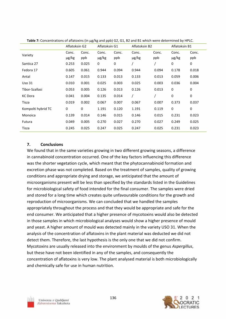
136
Table 7: Concentrations of aflatoxins (in µg/kg and ppb) G2, G1, B2 and B1 which were determined by HPLC.
Aflatoksin G2 Aflatoksin G1 Aflatoksin B2 Aflatoksin B1
Variety Conc.
µg/kg
Conc.
ppb
Conc.
µg/kg
Conc.
ppb
Conc.
µg/kg
Conc.
ppb
Conc.
µg/kg
Conc.
ppb
Santica 27 0.253 0.025 0 0 / / 0 0
Fedora 17 0.605 0.061 0.944 0.094 0.944 0.094 0.178 0.018
Antal 0.147 0.015 0.133 0.013 0.133 0.013 0.059 0.006
Uso 31 0.010 0.001 0.025 0.003 0.025 0.003 0.036 0.004
Tibor-Szallasi 0.053 0.005 0.126 0.013 0.126 0.013 0 0
KC Dora 0.041 0.004 0.135 0.014 / / 0 0
Tisza 0.019 0.002 0.067 0.007 0.067 0.007 0.373 0.037
Kompolti hybrid TC 0 0 1.191 0.120 1.191 0.119 0 0
Monoica 0.139 0.014 0.146 0.015 0.146 0.015 0.231 0.023
Futura 0.049 0.005 0.270 0.027 0.270 0.027 0.249 0.025
Tisza 0.245 0.025 0.247 0.025 0.247 0.025 0.231 0.023
7. Conclusions
We found that in the same varieties growing in two different growing seasons, a difference
in cannabinoid concentration occurred. One of the key factors influencing this difference
was the shorter vegetation cycle, which meant that the phytocannabinoid formation and
excretion phase was not completed. Based on the treatment of samples, quality of growing
conditions and appropriate drying and storage, we anticipated that the amount of
microorganisms present will be less than specified by the standards listed in the Guidelines
for microbiological safety of food intended for the final consumer. The samples were dried
and stored for a long time which creates quite unfavourable conditions for the growth and
reproduction of microorganisms. We can concluded that we handled the samples
appropriately throughout the process and that they would be appropriate and safe for the
end consumer. We anticipated that a higher presence of mycotoxins would also be detected
in those samples in which microbiological analyses would show a higher presence of mould
and yeast. A higher amount of mould was detected mainly in the variety USO 31. When the
analysis of the concentration of aflatoxins in the plant material was deducted we did not
detect them. Therefore, the last hypothesis is the only one that we did not confirm.
Mycotoxins are usually released into the environment by moulds of the genus Aspergillus,
but these have not been identified in any of the samples, and consequently the
concentration of aflatoxins is very low. The plant analysed material is both microbiologically
and chemically safe for use in human nutrition.
137
Acknowledgements
Luka Irenej Pečan, B. Sc. student was awarded 3th prize for this research work entitled
“Quantitative determination of biologically active compounds in industrial hemp (Cannabis
Sativa subsp. Sativa L.) and its Microbiological Quality” in 30th International competition of
young scientists “Step into the Future”. The competition was organized by the Bauman
Moscow State Technical University and the Russian Youth Engineering Society. The mentor
of the work was Marko Jeran and co-mentors Roman Štukelj and Karmen Godič Torkar.
The authors would like to thank the Slovenian Research Agency (ARRS) and the Ministry of
Agriculture, Forestry and Food Republic Slovenia for supporting the applicant CRP Project
No. V4-1611 and the Slovenian Research Agency for core funding No. P3-0388 and Projects
No. J1-9162, L3-2621. The authors thank the RN Institute, Ljubljana, for analytical support.
References
1. Štukelj R, Benčina M, Fanetti M, et al. Synthesis of stable cannabidiol (CBD)
nanoparticles in suspension. Mater Tehnol 2019; 53 (4): 543–549. doi:
10.17222/mit.2018.253
2. Amaducci S, Colauzzi M, Zatta A, Venturi G, Flowering dynamics in monoecious and
dioecious hemp genotypes. J Ind Hemp 2008; 13 (1): 5–19.
doi: 10.1080/15377880801898691
3. Andre CM, Hausman J-F, Guerriero G, Cannabis sativa: the plant of the thousand and
one molecules. Front Plant Sci 2016; 7: 1–17. doi: 10.3389/fpls.2016.00019
4. Ashton CH, Pharmacology and effects of cannabis: a brief review. Br J Psychiatry 2001,
178: 101–106. DOI: 10.1192/bjp.178.2.101
5. Elphick MR, Egertova M, The neurobiology and evolution of cannabinoid signalling.
Philos Trans R Soc Lond B Biol Sci 2001; 356 (1407): 381–408.
doi: 10.1098/rstb.2000.0787
6. Pertwee RG, The pharmacology of cannabinoid receptors and their ligands: an
overview. Int J Obes (Lond) 2006; 30 (1): S13–S18, doi: 10.1038/sj.ijo.0803272
7. Germano C, Baker S, Carl Germano, CNS, CDN: simple guide to the endocannabinoid
system, hemp phytocannabinoids/CBD and your health. Altern Ther Health Med 2020;
26 (S1): 32–34.
8. ISO 4833 (2003), Microbiology of food and animal feeding stuffs – Horizontal method
for the enumeration of microorganisms – Colony-count technique at 30 °C.
International Standard Organization, Brussels, Belgium, 1–6.
https://www.iso.org/standard/34524.html

138
9. ISO 16649-2 (2001), Microbiology of food and animal feeding stuffs — Horizontal
method for the enumeration of beta-glucuronidase-positive Escherichia coli — Part 2:
Colony-count technique at 44 degrees C using 5-bromo-4-chloro-3-indolyl beta-D-
glucuronide. International Standard Organization, Brussels, Belgium, 1–8.
https://www.iso.org/obp/ui/fr/#iso:std:iso:16649:-2:ed-1:v1:en
10. ISO 21527-1 (2008), Microbiology of food and animal feeding stuffs — Horizontal
method for the enumeration of yeasts and moulds — Part 1: Colony count technique
in products with water activity greater than 0.95. International Standard Organization,
Brussels, Belgium, 1–8. https://www.iso.org/standard/38275.html
11. ISO 6887-4 (2017), Microbiology of the food chain — Preparation of test samples,
initial suspension and decimal dilutions for microbiological examination — Part 4:
Specific rules for the preparation of miscellaneous products. Standard Organization,
Brussels, Belgium, 1–16. https://www.iso.org/standard/63338.html
12. ISO 6579-1 (2017), Microbiology of the food chain — Horizontal method for the
detection, enumeration and serotyping of Salmonella — Part 1: Detection of
Salmonella spp. International Standard Organization, Brussels, Belgium, 1–50.
https://www.iso.org/standard/56712.html
13. NLZOH, NVI (2019), Guidelines for the microbiological quality of food intended for the
final consumer (Slo. Smernice za mikrobiološko kakovost živil, ki so namenjena
končnemu potrošniku). In Rupel T, Lušicky M, Pavlica T, et al., editors. National
Laboratory for Health, Environment and Food, and Veterinary Faculty, University of
Ljubljana, Slovenia, 1–41.
14. Taghinasab M, Jabaji S, Cannabis microbiome and the role of endophytes in
modulating the production of secondary metabolites: an overview. Microorganisms
2020; 8 (3): 355. doi: 10.3390/microorganisms8030355
15. Kusari P, Kusari S, Lamshöft M, et al. Quorum quenching is an antivirulence strategy
employed by endophytic bacteria. Appl Microbiol Biotechnol 2014; 98 (16): 7173–
7183. doi: 10.1007/s00253-014-5807-3

139

140
_________________
In vitro cell experiments as important approach in cellular vesicles research Jan Zala1,* 1University of Ljubljana, Faculty of Health Sciences, Laboratory of Clinical Biophysics
Abstract: In the last years cellular vesicles (CVs) gain more and more interest in the scientific
community due to their specific characteristics. Research is focused on origin and function of
CVs, among which intercellular communication is the most interesting and promising.
Potential usage of CVs in diagnostic, therapy for different diseases and biotechnology is of
interest. Main reason why CVs are not yet used outside the research borders is problematic
analytics with poor robustness and low reliability of the results. To deepen knowledge about
CVs, different research approaches are used. CVs are monitored in in vitro and in vivo
processes. In this contribution, we will focus more on in vitro research with different cell
lines. Among vesiculation of the cells, also oxidative stress and inflammatory processes are
monitored to gain more information about cell development.
__________________

141
1. About cellular vesicles and in vitro cell experiments
It was suggested that cellular vesicles (CVs) are formed in the final stage of membrane
budding [1] by pinching off of the buds from the cell membranes and that they present an
intercellular communication system within the body [2,3]. CVs, discharged into the
circulation could assist with disposal of cellular waste products generated under stress
conditions and help the cells to preserve homeostasis [4]. CV formation by animal cells is
considered a physiological process [5] that can be accelerated by oxidative stress [6] and by
inflammation process [7]. CVs can be formed also by other organisms such as microalgae [8],
which are also more and more commonly used in CVs research in the last years. One of the
approaches for CVs research are in vitro cell experiments. In vitro studies are performed with
cells outside their normal biological context. It is important to establish and maintain high
standards of reproducibility and reliability when performing in vitro studies [9]. To improve
the quality of in vitro research, the concept of Good Cell Culture Practice was developed and
was widely adapted to ongoing scientific process [10]. Most commonly for in vitro studies
with cells, cancer cells are used.
Changes in in vitro cells, after being treated with CVs preparation, can be monitored in more
controlled conditions as when monitoring the in vivo changes. Among cell changes such as
cytotoxicity, oxidative stress and inflammation process [11], also vesiculation of in vitro cells
offers the information about cell response to different treatments. Also, in vitro
experiments are performed to evaluate the safety of EVs that may be therapeutically used.
2. Experiments on in vitro cells treated with preparations rich with vesicles
2.1. Cytotoxicity
For testing cytotoxicity, it is best to use different tests simultaneously to ensure better
reliability of the results. One of the most used cytotoxicity tests is uptake of the vital dye
neutral red (NR) assay provides quantitative estimation of viable cells number in a cell
culture. NR has properties of weak cationic dye, which can be retained in lysosomes only
when cell has an ability to maintain acidic pH. Test is based on the ability of viable cells to
absorb and bind the dye neutral red in the lysosomes. The absorbance of the dye is read
using a spectrophotometer [12].
Resazurin, or alamarBlue® is used as a cell health indicator - the redox reaction in resazurin-
based assays provides information about the intercellular processes and metabolic activity.
Resazurin undergoes a redox reduction to resorufin, a pink, fluorescent chemical which can
be detected via fluorescence or spectrophotometry [13]. Usually, NR and resazurin assays are
implemented together, because they can both be done on the same sample – first resazurin and then
NR assay is performed.
Trypan blue exclusion test is test for cell viability – it determines the number of viable cells
present in a cell suspension. Live cells possess intact cell membranes that exclude certain
dyes, such as trypan blue, eosin, or propidium, whereas dead cells do not. In Trypan blue
test, a cell suspension is treated with dye and then visually examined to determine whether
cells take up or exclude dye – examine and counting cells observed with microscope. It can

142
be seen that viable cells have a clear cytoplasm whereas a nonviable cells have a blue
cytoplasm [14].
With MTT (3-(4,5-dimethylthiazol-2-yl)-2,5-diphenyl tetrazolium bromide) assay cellular
metabolic activity is measured as an indicator of cell viability, proliferation and cytotoxicity.
This colorimetric assay is based on the reduction of a yellow tetrazolium salt - MTT to purple
formazan crystals by metabolically active cells. The quantity of the purple formazan crystals
is proportional to the number of living cells and is measured spectrophotometrically [15].
2. Oxidative stress
Oxidative stress is a phenomenon caused by an imbalance between production and
accumulation of oxygen reactive species (ROS): superoxide radicals (O2•-), hydrogen peroxide
(H2O2), hydroxyl radicals (•OH), and singlet oxygen (1O2), in cells and tissues and the ability of
a biological system to detoxify these reactive products. Oxidative stress is mentioned mostly
as harmful for human body, yet it is also exploited as a therapeutic approach to, with certain
degree of success, treat clinical conditions such as cancer [16]. CVs formation is considered
to be provoked by oxidative stress [6] and it is suggested that during oxidative stress,
oxidized proteins are formed, and cells release CVs as a compensatory mechanism to
remove them and to maintain homeostasis [17]. ROS are generated from both endogenous
(mainly produced by mitochondria, during both physiological and pathological conditions)
and exogenous sources - immune cell activation, inflammation, ischemia, infection, cancer,
excessive exercise, mental stress, and aging [16]. As research show oxidative stress can be
responsible for different diseases, i.e., cancer, diabetes, metabolic disorders, atherosclerosis,
and cardiovascular diseases [18].
Assay for ROS detection uses cell-permeant H2DCFDA which passively diffuses into cells and
is retained in the intracellular level after cleavage by intracellular esterases. Upon oxidation
by ROS, the nonfluorescent H2DCFDA is converted to the highly fluorescent 2', 7'-
dichlorofluorescein (DCF). Dead or dying cells produces ROS, therefore for detection of ROS
in living cells, propidium iodide (PI) or 7-AAD is used to evaluate ROS production only in
living cells which are PI/7-AAD negative. Fluorescence emission can be assessed by flow
cytometry, a standard fluorometer or fluorescence microscopy using appropriate filter [19].
Glutathione S-transferase (GST) are a family of antioxidant enzymes that act in antioxidant
defense, help in decreasing reactive oxygen species and in protecting cells from oxidative
stress [20]. It is one of the parameters, measured in connection with oxidative stress
occurrence - erythrocyte suspension GST activity has been proposed as a potential marker
for oxidative stress [21]. GST assay is measured spectrophotometrically [22].
Cholinesterase (ChE) is an enzyme needed for proper function of the nervous system, since it
is responsible for breaking down neurotransmitter acetylcholine that is believed to modulate
immune and anti-inflammatory response via the cholinergic system; a key factor in the anti-
inflammatory cholinergic pathway is supposed to be oxidative stress [23]. It was suggested
that decrease in erythrocyte suspension ChE activity may reflect an increased response of
the human body to oxidative stress [24]. For the detection of ChE activity,
spectrophotometric method adopted by Ellman [25] is used.

143
3. Inflammatory markers
Inflammation is a biological response of the immune system that can be triggered by
different factors, among which are pathogens, damaged cells and toxic compounds. These
factors can induce acute and/or chronic inflammatory responses that can result in tissue
damage or disease [26]. Systemic or acute-phase inflammation can be detected by
monitoring CRP production, stimulated by cytokines IL-6 and TNF-α, indicators of local
inflammatory response [27]. Inflammatory processes in connection with CVs are mostly
described for platelet-derived CVs (PCVs). PCV cargo can interact with cells involved in
inflammatory reactions. Also, increase in blood PCV levels has been reported in
inflammatory-associated disorders. Proinflammatory action of PCVs modulates several
processes, including activation of both immune cells and endothelium. Moreover, PCVs is
considered to be a rich potential source of proinflammatory cytokines and complement
components [28].
Interleukin-6 (IL-6) is a myokine which acts as an inflammatory mediator [29]. Tumor
necrosis (TNF-∝) was originally described as a circulating factor that can cause necrosis of
tumors but has since been identified as a key regulator of the inflammatory response [30].
Also, inflammatory cytokine interleukin 1- 𝛽 (IL-1𝛽) is of interest, since it is an important
regulator of inflammation with controlling many innate immune processes. For
measurement of cytokines in samples, commercial ELISA kits are used.
4. Isolation and characterization of cellular vesicles
Cell-derived vesicles from eukaryotic cells are considered to be important intercellular
“multipurpose carriers” involved in communication, protection against external and internal
cellular stress and in the exchange of genetic information [31].
There are many known strategies for isolation of the in vitro cell-derived vesicles. Different
authors describe different approaches for CVs isolation: using precipitation kits
(ExoQuickTM [32], Total Exosome IsolationTM [33]), differential centrifugation including
ultracentrifugation (UC) [34], filtration [35], density gradient UC [35], sucrose cushion UC
[36], custom charge-based precipitation method [37]. After CVs isolation, different
approaches are used for characterization and analysis of CVs: transmission electron
microscopy (TEM) [20] or immunogold TEM [38], flow cytometry [39], western blot [23],
nanoparticle tracking analysis (NTA), atomic force microscopy (AFM) [34], fluorescence
microscopy [40], dynamic light scattering (DLS) [38], bicinchoninic acid (BCA) assay [38],
Bradford assay [35], RNA [39], proteomics [41], custom colorimetric nanoplasmonic assay
(molar concentration)[34], zeta potential [42], quantitative real-time polymerase chain
reaction (qRT-PCR) [43,44].
5. Conclusions
Every new approach and method are an important contribution in understanding formation
and role of CVs in human body and a step closer to new era of diagnostics and therapy.
Monitoring response of in vitro cells on treatment with preparations rich with CVs can offer

144
improvement of protocols for diagnostics and therapy in vivo. With appropriate isolation and
analysis of isolates from in vitro cells, CVs formation mechanisms can be better understood.
References
1. Hurley JH, Boura E, Carlson LA, Różycki B. Membrane budding. Cell. 2010; 143(6):875-
87. doi:10.1016/j.cell.2010.11.030
2. Sorkin R, Huisjes R, Bošković F, et al. Nanomechanics of Extracellular Vesicles Reveals
Vesiculation Pathways. Small. 2018; 14(39):e1801650. doi:10.1002/smll.201801650
3. Oszvald Á, Szvicsek Z, Sandor GO, et al. Extracellular vesicles transmit epithelial growth
factor activity in the intestinal stem cell niche. Stem Cells. 2020; 38(2):291-300.
doi:10.1002/stem.3113
4. Frühbeis C, Helmig S, Tug S, Simon P, Krämer-Albers EM. Physical exercise induces
rapid release of small extracellular vesicles into the circulation. J Extracell Vesicles.
2015; 4:28239. doi:10.3402/jev.v4.28239
5. Morshed A, Karawdeniya BI, Bandara YMND, Kim MJ, Dutta P. Mechanical
characterization of vesicles and cells: A review. Electrophoresis. 2020;
doi:10.1002/elps.201900362
6. Borras C, Mas-Bargues C, Sanz-Ros J, et al. Extracellular vesicles and redox modulation
in aging. Free Radic Biol Med. 2020; 149:44-50.
doi:10.1016/j.freeradbiomed.2019.11.032
7. Chaar V, Romana M, Tripette J, et al. Effect of strenuous physical exercise on
circulating cell-derived microparticles. Clin Hemorheol Microcirc. 2011; 47(1):15-25.
doi:10.3233/CH-2010-1361
8. Picciotto S, Barone ME, Fierli D, et al. Isolation of extracellular vesicles from
microalgae: towards the production of sustainable and natural nanocarriers of
bioactive compounds. Biomater Sci. 2021; doi:10.1039/d0bm01696a
9. Hirsch C, Schildknecht S. Research Reproducibility: Keeping Up High Standards. Front
Pharmacol. 2019; 10:1484. doi:10.3389/fphar.2019.01484
10. Coecke S, Balls M, Bowe G, et al. Guidance on good cell culture practice. a report of the
second ECVAM task force on good cell culture practice. Altern Lab Anim. 2005;
33(3):261-87. doi:10.1177/026119290503300313
11. Jan Z, Drab M, Drobne D, et al. Decrease in Cellular Nanovesicles Concentration in
Blood of Athletes More Than 15 Hours After Marathon. Int J Nanomedicine. 2021;
16:443-456. doi:10.2147/IJN.S282200
12. Repetto G, del Peso A, Zurita JL. Neutral red uptake assay for the estimation of cell
viability/cytotoxicity. Nat Protoc. 2008; 3(7):1125-31. doi:10.1038/nprot.2008.75
13. Pace RT, Burg KJ. Toxic effects of resazurin on cell cultures. Cytotechnology. 2015;
67(1):13-7. doi:10.1007/s10616-013-9664-1
14. Strober W. Trypan Blue Exclusion Test of Cell Viability. Curr Protoc Immunol. 2015;
111:A3.B.1-A3.B.3. doi:10.1002/0471142735.ima03bs111
145
15. Śliwka L, Wiktorska K, Suchocki P, et al. The Comparison of MTT and CVS Assays for the
Assessment of Anticancer Agent Interactions. PLoS One. 2016; 11(5):e0155772.
doi:10.1371/journal.pone.0155772
16. Pizzino G, Irrera N, Cucinotta M, et al. Oxidative Stress: Harms and Benefits for Human
Health. Oxid Med Cell Longev. 2017; 2017:8416763. doi:10.1155/2017/8416763
17. Yarana C, St Clair DK. Chemotherapy-Induced Tissue Injury: An Insight into the Role of
Extracellular Vesicles-Mediated Oxidative Stress Responses. Antioxidants (Basel). 2017;
6(4)doi:10.3390/antiox6040075
18. Ray PD, Huang BW, Tsuji Y. Reactive oxygen species (ROS) homeostasis and redox
regulation in cellular signaling. Cell Signal. 2012; 24(5):981-90.
doi:10.1016/j.cellsig.2012.01.008
19. Ameziane-El-Hassani R, Dupuy C. Detection of Reactive Oxygen Species in Cells
Undergoing Oncogene-Induced Senescence. Methods Mol Biol. 2017; 1534:139-145.
doi:10.1007/978-1-4939-6670-7_13
20. Mergani A, Mansour AA, Askar T, et al. Glutathione S-Transferase Pi-Ile 105 Val
Polymorphism and Susceptibility to T2DM in Population from Turabah Region of Saudi
Arabia. Biochem Genet. 2016; 54(4):544-551. doi:10.1007/s10528-016-9740-2
21. Neefjes VM, Evelo CT, Baars LG, Blanco CE. Erythrocyte glutathione S transferase as a
marker of oxidative stress at birth. Arch Dis Child Fetal Neonatal Ed. 1999; 81(2): F130-
133. doi:10.1136/fn.81.2.f130
22. Mannervik B. The isoenzymes of glutathione transferase. Adv Enzymol Relat Areas Mol
Biol. 1985; 57:357-417. doi:10.1002/9780470123034.ch5
23. Villeda-Gonzalez JD, Gómez-Olivares JL, Baiza-Gutman LA, et al. Nicotinamide reduces
inflammation and oxidative stress via the cholinergic system in fructose-induced
metabolic syndrome in rats. Life Sci. 2020;250:117585. doi:10.1016/j.lfs.2020.117585
24. Duchnowicz P, Ziobro A, Rapacka E, Koter-Michalak M, Bukowska B. Changes in
Cholinesterase Activity in Blood of Adolescent with Metabolic Syndrome after
Supplementation with Extract from. Biomed Res Int. 2018; 2018:5670145.
doi:10.1155/2018/5670145
25. ELLMAN GL, COURTNEY KD, ANDRES V, FEATHER-STONE RM. A new and rapid
colorimetric determination of acetylcholinesterase activity. Biochem Pharmacol. 1961;
7:88-95. doi:10.1016/0006-2952(61)90145-9
26. Chen L, Deng H, Cui H, et al. Inflammatory responses and inflammation-associated
diseases in organs. Oncotarget. 2018; 9(6):7204-7218. doi:10.18632/oncotarget.23208
27. Petersen AM, Pedersen BK. The anti-inflammatory effect of exercise. J Appl Physiol
(1985). 2005; 98(4):1154-62. doi:10.1152/japplphysiol.00164.2004
28. Słomka A, Urban SK, Lukacs-Kornek V, Żekanowska E, Kornek M. Large Extracellular
Vesicles: Have We Found the Holy Grail of Inflammation? Front Immunol. 2018;
9:2723. doi:10.3389/fimmu.2018.02723
146
29. Mendham AE, Donges CE, Liberts EA, Duffield R. Effects of mode and intensity on the
acute exercise-induced IL-6 and CRP responses in a sedentary, overweight population.
Eur J Appl Physiol. 2011; 111(6):1035-45. doi:10.1007/s00421-010-1724-z
30. Bradley JR. TNF-mediated inflammatory disease. J Pathol. 2008; 214(2):149-60.
doi:10.1002/path.2287
31. Nieuwland R, Sturk A. Why do cells release vesicles? Thromb Res. 2010; 125 Suppl
1:S49-51. doi:10.1016/j.thromres.2010.01.037
32. Brandon-Warner E, Feilen NA, Culberson CR, et al. Processing of miR17-92 Cluster in
Hepatic Stellate Cells Promotes Hepatic Fibrogenesis During Alcohol-Induced Injury.
Alcohol Clin Exp Res. 2016; 40(7):1430-1442. doi:10.1111/acer.13116
33. Raji GR, Sruthi TV, Edatt L, Haritha K, Sharath Shankar S, Sameer Kumar VB. Horizontal
transfer of miR-106a/b from cisplatin resistant hepatocarcinoma cells can alter the
sensitivity of cervical cancer cells to cisplatin. Cell Signal. 2017; 38:146-158.
doi:10.1016/j.cellsig.2017.07.005
34. Berardocco M, Radeghieri A, Busatto S, et al. RNA-seq reveals distinctive RNA profiles
of small extracellular vesicles from different human liver cancer cell lines. Oncotarget.
2017; 8(47):82920-82939. doi:10.18632/oncotarget.20503
35. He M, Qin H, Poon TC, et al. Hepatocellular carcinoma-derived exosomes promote
motility of immortalized hepatocyte through transfer of oncogenic proteins and RNAs.
Carcinogenesis. 2015; 36(9):1008-1018. doi:10.1093/carcin/bgv081
36. Kapoor NR, Chadha R, Kumar S, Choedon T, Reddy VS, Kumar V. The HBx gene of
hepatitis B virus can influence hepatic microenvironment via exosomes by transferring
its mRNA and protein. Virus Res. 2017; 240:166-174.
doi:10.1016/j.virusres.2017.08.009
37. Deregibus MC, Figliolini F, D'Antico S, et al. Charge-based precipitation of extracellular
vesicles. Int J Mol Med. 2016; 38(5):1359-1366. doi:10.3892/ijmm.2016.2759
38. Povero D, Eguchi A, Niesman IR, et al. Lipid-induced toxicity stimulates hepatocytes to
release angiogenic microparticles that require Vanin-1 for uptake by endothelial cells.
Sci Signal. 2013; 6(296):ra88. doi:10.1126/scisignal.2004512
39. Takahashi K, Yan IK, Kogure T, Haga H, Patel T. Extracellular vesicle-mediated transfer
of long non-coding RNA ROR modulates chemosensitivity in human hepatocellular
cancer. FEBS Open Bio. 2014; 4:458-467. doi:10.1016/j.fob.2014.04.007
40. Chen L, Brigstock DR. Integrins and heparan sulfate proteoglycans on hepatic stellate
cells (HSC) are novel receptors for HSC-derived exosomes. FEBS Lett. 2016;
590(23):4263-4274. doi:10.1002/1873-3468.12448
41. Cho YE, Im EJ, Moon PG, Mezey E, Song BJ, Baek MC. Increased liver-specific proteins
in circulating extracellular vesicles as potential biomarkers for drug- and alcohol-
induced liver injury. PLoS One. 2017; 12(2):e0172463.
doi:10.1371/journal.pone.0172463

147
42. Chen L, Charrier A, Zhou Y, et al. Epigenetic regulation of connective tissue growth
factor by MicroRNA-214 delivery in exosomes from mouse or human hepatic stellate
cells. Hepatology. 2014; 59(3):1118-1129. doi:10.1002/hep.26768
43. Lambrecht J, Jan Poortmans P, Verhulst S, Reynaert H, Mannaerts I, van Grunsven LA.
Circulating ECV-Associated miRNAs as Potential Clinical Biomarkers in Early Stage HBV
and HCV Induced Liver Fibrosis. Front Pharmacol. 2017; 8:56.
doi:10.3389/fphar.2017.00056
44. Lv LH, Wan YL, Lin Y, et al. Anticancer drugs cause release of exosomes with heat shock
proteins from human hepatocellular carcinoma cells that elicit effective natural killer
cell antitumor responses in vitro. J Biol Chem. 2012; 287(19):15874-15885.
doi:10.1074/jbc.M112.340588

148

149
__________________
Music and protocol
Kušej Gala Nina *
Abstract
The article Music and Protocol examines the role of music in protocol and its effect on the
listener. It systematically sums up standard protocol occasions as well as standard music
pieces that are being used during ceremonies. In connection with that, the Police Orchestra
as the official protocol orchestra of the Republic of Slovenia is briefly presented.
Furthermore, the article stresses state celebrations as the freest performative platform in
terms of protocol music and - last but not least - in connection with that emphasizes the
importance of the performative context on the listener’s qualitative perception of music and
ceremonies in general.
__________________

150
1. Introduction
Protocol by definition means a set of formal and social rules of interaction between official
state representatives. Consequently protocol music presents the means of achieving these
rules 1.
Music as a protocol element represents a notable part of a ceremonial, as it helps to frame it
and has the ability to structurally dictate the course of action through sound and its form. At
the same time, it has the power to emotionally impact the individual and in such way
underline the true meaning of an individual protocol occasion or event.
Music has always had an important role in protocol as well as in diplomacy. The contextual
area of using music in this way is extensive and includes a wide range of various protocol
events, from strictly prescribed ceremonials (such as a reception of a foreign statesman
during an official visit), to freer ceremonial forms (such as a state celebration) 2. No matter
the form, required for an individual event, a necessary constant of such music is its message
and its effect on the listener, be it to strengthen national consciousness, glorify authority or
something else connected with »protocol«. So it is about music as a protocol element, which
is actually music in a specific function that fulfills its role to the fullest extent only when
placed within an institution or context. The signal function of the military horn would not
fulfill its actual role outside a military battle, just as a composition at a state celebration
would not fulfill its actual function without the set design or visual framing, the right
opportunity for a performance and an audience it can address.
2. Music as a key structural element of protocol events
Despite the fact that contemporary protocol of Central Europe is mostly modernized,
simplified and minimized, the traditional foundations are still visible in the primary goals of
the ceremonial, which remain largely, above all the element of music, consistently aimed at
glorifying the state, raising the national consciousness and paying homage to foreign
statesmen, while at the same time performing a signaling function (performance of an elegy
by a wind instrument ensemble during a ceremonial wreath laying is for example a sign for
the president of the republic to start walking behind the wreath bearers towards the
memorial). Protocol remains the organizational foundation for the functioning of the state
apparatus and managing the relations between individuals within this framing.
While the strict ceremonial preserves the use of traditional music forms (national anthems,
marching songs), more contemporary ceremonials, such as various receptions and state
celebrations, use a broad specter of musical and other means of expression as part of the
contemporary language of diplomacy 2. So this is a process of combining tradition,
symbolizing national identity, with the contemporary, symbolizing the future. The above
stated combination of elements as an efficient recipe to increase popular support can often
be seen in diplomatic practices of various statesmen.
An interesting example of one such combination was the enthronement of the new Dutch
king Willem-Alexander in 2013, which almost went awry at first glance, but in the end turned
to his advantage. First the media 3 practically tore the official crowning to pieces as soon as

151
the lyrics were published, claiming that the lyrics are daft. Even the fact that this popular
ballad was supposed to be carried out by some local celebrities did not help. A petition was
also launched in the Netherlands as part of the general dislike of the song. After the
inauguration ceremony the situation changed rapidly in favor of the new king, because he
also went to the concert of the world famous and very popular Dutch DJ Armin van Buuren
with the Royal Concertgebouw Orchestra with his wife and children 4. Joining tradition
(symbolized by the symphony orchestra) and popular music (in form of electronic music)
turned out to be a great success, especially because it was supported with somewhat
populist statements, which the king gave in his ceremonial speech after the inauguration,
where he also talked about how he should be addressed: »I don't care, people can address
me as they wish, as long as it makes them feel good.« 5.
The current President of the Republic of Slovenia Borut Pahor has been using similar
principles lately, in general keeping the formal framing of the ceremonial, but "softening"
and popularizing it when this is possible, often helping in this process himself. A popular rock
band performed at the award ceremony for Jabolko navdiha (The apple of inspiration)1,
which was awarded to the drummer of the band Elvis Jackson Marko Soršak - Soki for his
contribution to child music literacy. They were joint on stage by the president himself:
"Pahor the all-rounder joined the band Big Foot Mama on stage and played the song Nisem
več s tabo with them. He played the drums with drumsticks given to him by the drummer of
the band Elvis Jackson, Marko Soršak - Soki.« 6.
The former US president Barack Obama went even one step further towards popularizing
the protocol, as he gave an iPod to the Queen of the United Kingdom Elizabeth II (a political
figure personifying tradition) as part of the traditional protocol act of exchanging gifts in
2009. On the iPod were photos of her visit to Washington and Virginia and also 40 popular
Broadway songs, among them The King and I, West Side Story and Dreamgirls 6. With this
gesture he was innovative in combining a photo album (a normal gift for such occasions) and
a standard music storage medium (CD) in a product of American technology that symbolizes
looking to the future and patriotism.
3. Police orchestra of the Republic of Slovenia as the official protocol orchestra
The Slovene Police Orchestra was established in 1948 and has been active to this day under
different names, political regimes and state regulations, performing in formal state
circumstances. Since the independence of the Republic of Slovenia in 1991 it has also
officially become the state protocol orchestra and has ever since had a significant role in
Slovene State Protocol. After gaining its independence, Slovenia had to create the
foundations of a new state protocol and thereby define the role and the repertoire of the
protocol orchestra during ceremonial events 7.
Protocol events, which are based on an established ceremonial with the corresponding
music forms, are mostly performed by the Police Orchestra. During such events the
1 Jabolko navdiha is an award, given by the President of the Republic of Slovenia at a ceremonial, similar to a
presidential commendation.

152
orchestra usually appears and performs together with the Guard of Honour of the Slovene
Armed Forces. When united, the two formations are officially addressed as the Honorary
Unit of the Republic of Slovenia 8.
Most standard in terms of the musical form and at the same time the most frequently
performed musical pieces by the Police Orchestra are: anthems, marches, mourning songs
and solo performances of trumpeters. These are being regularly used in standard protocol
events such as: welcome receptions with military honours, inspections of the Guard of
Honour, wreath laying ceremonies, receptions, etc 8.
State celebrations present a wider and above all more versatile field of creative performing
options for the Police Orchestra, where the repertoire of the orchestra is not limited to the
usual standard musical literature 2.
4. Music of state celebrations
At the more relaxed events, among which the cultural programs of state celebrations are the
most expressive, there are basically only few (but important) restrictions – the principles of
moderation, adequacy and appropriateness.
The latter (cultural parts of state celebrations) vary and are characterized by, among other
factors, different producing and directing approaches to how the event is structured, which
defines the role of music as a structural element of each individual celebration. This also
defines the work of the music composer or author, as the concept of the celebration
determines, if a certain composition or piece will be performed in the original or as an
adaptation, and if the music is serving as the background or central element of the event. In
any case the music at state celebration events can be comprehensively presented only in the
context of the other structural elements, which applies not only to state celebrations, but to
protocol music in general, which actually categorizes it as a musical genre 2.
5. The crucial meaning of the performative context for the protocol music genre
Considering the fact that music is »neutral« in its original form and something we all share, it
gets its connotation only when performed with a specific background, having a role in
various situations or becoming part of the collective memory. In an example from WWII,
given by Jessica Gienow-Hecht 9, a decorated US pilot had supposedly refused to bomb a
city, in which Beethoven was born and educated. In reference to music as a universal
language, Kathleen M. Higgins 9 is of the opinion that we all, regardless our differences and
the diversity of our music, sound human.
In the first place, protocol music needs to be performed in certain objective circumstances
(location, music cast, etc.) for being able to impact the listener. Furthermore, the intensity of
its message is substantially defined by the context in which it is being performed. The term
context should be understood as a social, emotional or ambiental category which has the
capacity to determine the quality of the musical experience.
A very indicative example of the stated theory can be a musical piece originally performed by
an Oberkrainer musical band. The chosen musical example can reach into entirely different
emotional range of the listener if it's being performed in the Oberkrainer context (typical

153
musical cast, instruments, outfit of the performers and environment) in comparison with a
situation, in which just the music itself is being extracted and installed into an entirely
different context, for example a state celebration. In such case, the originally »mocking«
character of the musical piece transforms into something entirely different, perhaps even
solemn and glamorous as the context of state celebrations actually is 2.
In certain cases, it is not the ceremonial that dictates the music, but the other way around,
which means that certain music can become some sort of »parastatal protocol element« in
certain circumstances. A picturesque example of the above is the Slovenian »local patriotic«
song Vstajenje Primorske2. This composition is considered a sort of unofficial anthem among
the people of the Primorska region and often evokes stronger emotions than the official
national anthem, as the audience often stand up when it is played, place their right hand on
their hearts and sing the lyrics in unison. As Felicity Laurence 9 states, music can be a
strong instrument of propaganda. Primarily in such cases as the above mentioned
composition, caution is needed so patriotism does not turn into nationalism, political
incitement or a way of dividing people.
In the context of sports, which (this applies very much to Slovenia) can unify a nation, the
danger of misuse for propaganda is slightly smaller. The song Slovenija gre naprej3 for
instance, became an informal anthem of the Slovenia national football team. The song still
evokes feelings of unity and patriotism in its most positive form.
6. Conclusion
Music in the function of or as a protocol element represents one of the building blocks of an
individual protocol event or ceremonial. It is music that cannot exist by itself and cannot
fulfill its function by itself, but has its practical function and conveys a message only within
the protocol framework. Therefore, its artistic value can only be discussed within its context.
At the same time, it is music that is absolutely and inseparably tied to the event; it is subject
to the event in a way and supports it. After all, fanfares cannot truly exist without a ruler and
there in no real point in state celebration without an audience.
References
1. Kušej NG, Glasba kot protokolarni element, Protokol. 2016. Muzikološki zbornik. 2021;
53:267-268, http://bos.zrc-sazu.si/cgi/a03.exe?name=sskj_testa&expression=
protokol&hs=1.
2. Kušej NG, Glasba kot protokolarni element. Master's degree thesis. Ljubljana,
Filozofska fakulteta, Oddelek za muzikologijo, 2016.
2 The song »Vstajenje Primorske,« was set to music and adapted by Rado Simoniti in 1968 for the celebration of
the 25th anniversary of the general rebellion in the Primorska region at the fall of fascism. 3 The song »Slovenija gre naprej« was written in 2000 by Zoran Predin, Peter Lovsin and Vlado Kreslin for the
European football championship in Belgium and the Netherlands.

154
3. MMC RTV Slovenija. 2013a. »Foto: “Naj živi kralj!” Viljem Aleksander je ustoličen.«
Accessed on 10 June 2021, https://www.rtvslo.si/svet/foto-naj-zivi-kralj-viljem-
aleksander-je-ustolicen/307797.
4. A State of Trance. 2013. »King and Queen of The Netherlands surprise Armin van
Buuren.« Accessed on 10 June 2021, http://www.astateoftrance.com/news/king-and-
queen-of-the-netherlands-surprise-armin-van-buuren/.
5. 24ur.com. 2013. »Nizozemska kljub kritikam ostaja pri pesmi za ustoličenje kralja.«
Accessed on 10 June 2021, http://www.24ur.com/ekskluziv/zanimivosti/nizozemska-
kljub-kritikam-ostaja-pri-pesmi-za-ustolicenje-kralja.html.
6. MMC RTV Slovenija. 2015. »Foto: Koncert v predsedniški palači – za bobni pa Borut
Pahor.« Accessed on 10 June 2021, http://www.rtvslo.si/zabava/druzabna-
kronika/foto-koncert-v-predsedniski-palaci-za-bobni-pa-borut-pahor/362775.
7. Kolenc T, Od Godbe ljudske milice do protokolarnega orkestra: 50 let delovanja
Policijskega orkestra. 1999, Ministrstvo za notranje zadeve, Urad za javno varnost,
Ljubljana.
8. Kušej NG, Private archive of the amployee of the Protocol of the Republic of Slovenia.
9. Ahrendt R, Ferraguto M, Mahiet D, . 2014. »Introduction.« In Music and Diplomacy
from the Early Modern Era to the Present, edited by Rebekah Ahrendt, Mark Ferraguto
and Damien Mahiet, 1–16. New York: Palgrave Macmillan.

155

156
__________________
The role of painting in the life and works of Fyodor Mikhailovich Dostoevsky
Prelovšek Anita*
Abstract
This article, as a contribution to the bicentenary of the birth of Fyodor Mikhailovich
Dostoevsky, describes the way in which the art of painting was important for the writer’s life,
mentioning his favourite paintings and describing how they and the art of painting in general
are reflected in his works. Especially during the years he spent abroad, Dostoevsky was a
regular visitor to art galleries. In St Petersburg, he frequently went to the Ermitage and
visited exhibitions of new works by Russian painters. He also published two articles
containing his critical opinions about exhibitions he visited in Russia. In its last part, the
article briefly quotes some modern examples of painting or drawing relating to the life and
work of Dostoevsky.
__________________

157
1. Introduction
Dostoevsky admired all forms of art, included painting. He was a regular visitor to the
Ermitage and attended the exhibitions of paintings organized every year in the Academy of
Arts in St Petersburg, where he was informed about new works by the most important
Russian painters. He expressed his opinions about exhibitions in two articles, published in his
Diary of a Writer. During his stays abroad (1867‐71), he was a keen patron of galleries in
European cities such as Dresden, Basle, Florence, Venice and Bologna. He had his favourite
painters and paintings which he never tired of seeing again and again. He retained the
impressions that examples of the visual art made on him and used them to depict some of
the characters, scenes, feelings and philosophical ideas in his novels and short stories. In
some of his works he also makes explicit mention of certain paintings.
2. Dostoevsky’s favourite paintings and their place in his works
2.1. Paradise on Earth
Coastal landscape with Acis and Galatea (Figure 1), a work by Claude Lorrain, a French
painter of the baroque era, was for Dostoevsky a representation of a paradise on Earth. He
was particularly fond of it, mentioning it three times in his works: in his novels The Raw
Youth and The Possessed (The Devils) and also in The Dream of a Ridiculous Man, a short
story.
The painting represents an episode from an ancient Greek mythological story used by Ovid in
Metamorphoses. It tells the story of Galatea, a sea nymph (the first of the fifty Nereids), who
refused the attentions of the cyclops Polyphemus and fell in love with Acis. When
Polyphemus saw Galatea in the arms of Acis, he killed his rival with a rock, who after his
death transformed himself into a river [1].
Claude Lorrain,4 who spent much of his life in Italy, where he was inspired by its nature and
art, was famous for painting landscapes and portraying mythological or biblical subjects. In
this painting, he depicts an idyllic landscape on the seashore, where Acis and Galatea are
enjoying their love. The beauty of nature surrounds the protagonists, who are hidden from
the eyes of Polyphemus. On the right side of the painting, on one of the rocks above the
shore, we can see the jealous Polyphemus playing on a flute. This is a typical romantic topic
showing an idyllic landscape, where everything is in harmony, a pastoral scene par
excellence, from which all troubles and the final catastrophe seem far removed.
4 He was born under the name Claude Gellée, taking the pseudonym Claude Lorrain because of his being born in
the Duchy of Lorraine [2].

158
Figure 1. Claude Lorrain: Coastal landscape with Acis and Galatea (1657) [3].
Dostoevsky named this painting »The Golden Age«. A hero from the novel The Raw Youth,
Versilov, gives it this title and says he saw it in his dreams, though not as a painting but as a
reality, the picture serving as a description of a paradise [4].
The same description of a Garden of Eden on Earth that appeared in The Raw Youth (1875)
was originally intended to replace the chapter »At Tikhon's« that had been censored5 out of
a previous novel, The Possessed (The Devils) (1872).
»A corner of the Greek Archipelago; blue caressing waves, islands and rocks; fertile shore, a
magic vista on the horizon, the appeal of the setting sun – no words could describe it. Here
was the cradle of European man, here were the first scenes of the mythological world, here
its green paradise. … Here had once lived a beautiful race. They rose and went to sleep happy
5 In this chapter the hero, Stavrogin, confesses to the monk Tikhon the sin he has committed, abusing a
vulnerable young girl. The chapter had been censored by Mikhail Katkov, editor of The Russian Messenger,
where the novel was first published. In modern editions of The Possessed (The Devils) this chapter is usually
included (as a Chapter 9 in the second part of the novel or as an appendix) [6]. It has also been published
separately, as in the celebrated translation by S. S. Koteliansky and Virginia Woolf [5].

159
and innocent; they filled the woods with their joyful songs; the great abundance of their
virgin powers went out into love and into simple happiness. The sun bathed these islands and
sea in its beams, rejoicing in its beautiful children. Wonderful dream, splendid illusion! A
dream the most incredible of all that had ever been dreamt, but upon it the whole of
mankind has lavished all its powers throughout history; for this men have died on the cross
and their prophets have been killed; without this, nations will not live and are unable even to
die. I lived through all these feelings in my dream; I do not know what exactly I dreamt about,
but the rocks, the sea, and the slanting rays of the setting sun – all these seemed to be still
visible to me, when I woke and opened my eyes, fort he first time in my life, found them full of
tears. A feeling of happiness, until then unfamiliar to me, went through my whole heart, even
painfully. […]« [5].
A painting by Claude Lorrain also has the same function of depicting a paradise on Earth in
the short story The Dream of a Ridiculous Man (1877):
I came to stand on this other earth, in the bright light of a sunny day, lovely as paradise. I was
standing, it seems, on one of those islands which on our earth make up the Greek
archipelago, or somewhere on the coast of the mainland adjacent to that archipelago. Oh,
everything was exactly as with us, but seemed everywhere to radiate some festivity and a
great, holy, and finally attained triumph. The gentle emerald se splashed softly against the
shores and kissed them with love - plain, visible, almost conscious. Tall, beautiful trees stood
in all the luxury of their flowering, and their numberless leaves, I was convinced, greeted me
with their soft, gentle sound, as if uttering words of love. The grass glittered with bright,
fragrant flowers. Flocks of birds flew about in the air and, fearless of me, landed on my
shoulders and arms, joyfully beating me with their dear, fluttering wings. And finally I got to
see and know the people of that happy earth. They came to me themselves, they surrounded
me, kissed me. Children of the sun, children of their sun - oh, how beautiful they were! Never
on earth have I seen such beauty in man. Maybe only in our children, in their first years, can
one find a remote, though faint, glimmer of that beauty. The eyes of these happy people
shone with clear brightness. Their faces radiated reason and a sort of consciousness fulfilled
to the point of serenity, yet they were mirthful faces; a childlike joy sounded in the words and
voices of these people. Oh, at once, with the first glance at their faces, I understood
everything, everything! This was the earth undefiled by the fall, the people who lived on it
had not sinned, they lived in the same paradise in which, according to the legends of all
mankind, our fallen forefathers lived, with the only difference that the whole earth here was
everywhere one and the same paradise. These people, laughing joyfully, crowded around me
and caressed me; they took me with them and each of them wished to set me at ease. Oh,
they didn’t ask me about anything, but it seemed to me as if they already knew everything,
and wished quickly to drive the torment from my face. [7].

160
2.2. The Ideal of Beauty
Dostoevsky felt very highly of the art of Raphael Sanzio and considered his Sistine Madonna
(Figure 2) to be the best work of this renaissance master [8].
This vast oil painting (265 cm x 196 cm) represents Maria holding in her arms a baby Christ
surrounded by St Barbara and St Sixtus. At the bottom of the painting there are two cherubs
with wings [9]. Today these two cherubs are the most famous part of the painting, being
represented on a range of souvenirs and objects. It was commissioned in 1512 by Pope Julius
for the basilica of San Sisto in Piacenza, and in 1754, it was sold to a Polish king and taken to
Dresden. During the Second World War, it was saved from the bombing of the city and
removed to Moscow. Until 1955 it had been exposed in the Pushkin State Museum of Fine
Arts and then returned to Dresden [10].
This picture became one of the most famous representations of the Madonna. Numerous
European and Russian intellectuals and artists expressed their enthusiasm about it, among
them Dostoevsky. In his novel The Possessed (The Devils) Dostoevsky named the Sistine
Madonna »Queen of Queens, that ideal of humanity« [11]. As Dostoevsky’s wife Anna
Grigorevna writes in her memoirs, during their stay in Dresden they visited the gallery and
Dostoevsky, of all of the exposition rooms, immediately took her to the one displaying the
Sistine Madonna. This painting was for him »the highest manifestation of the human genius«
and »he was able to stand in front of this picture for hours and hours, moved to tears« [8].6
Dostoevsky’s contemporaries testify that the writer loved this painting so much that a copy
of it always hung above his bed in his apartment in St Petersburg [13].
6 For example, in an article about this painting, the Russian poet Vasily Zhukovsky (1783-
1852) mentions »a genius of pure beauty« [12].
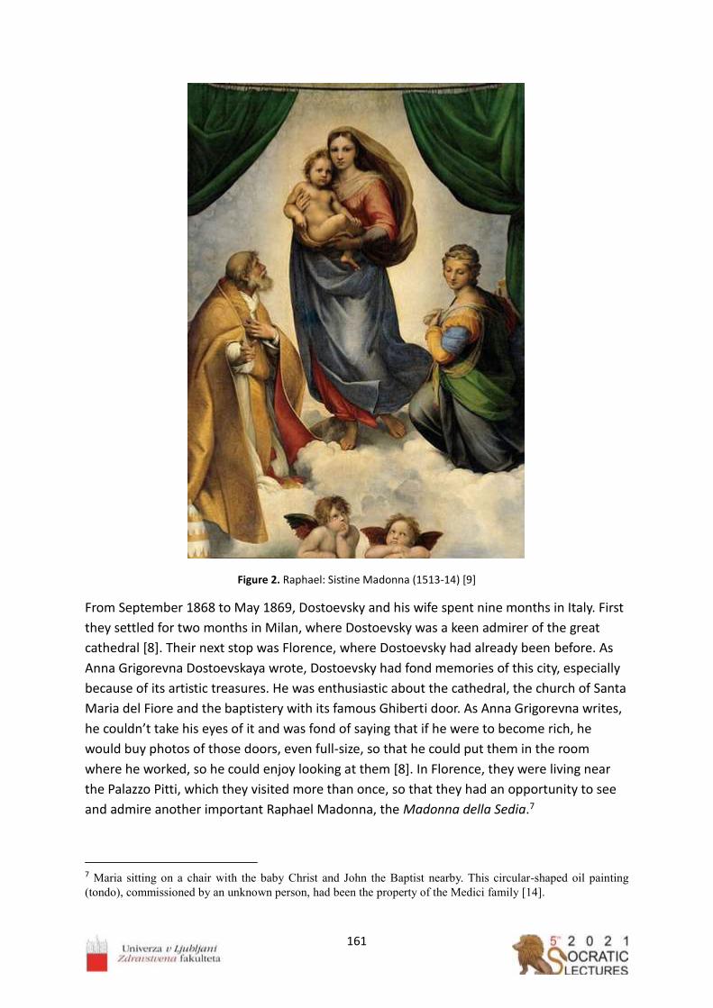
161
Figure 2. Raphael: Sistine Madonna (1513‐14) [9]
From September 1868 to May 1869, Dostoevsky and his wife spent nine months in Italy. First
they settled for two months in Milan, where Dostoevsky was a keen admirer of the great
cathedral [8]. Their next stop was Florence, where Dostoevsky had already been before. As
Anna Grigorevna Dostoevskaya wrote, Dostoevsky had fond memories of this city, especially
because of its artistic treasures. He was enthusiastic about the cathedral, the church of Santa
Maria del Fiore and the baptistery with its famous Ghiberti door. As Anna Grigorevna writes,
he couldn’t take his eyes of it and was fond of saying that if he were to become rich, he
would buy photos of those doors, even full‐size, so that he could put them in the room
where he worked, so he could enjoy looking at them [8]. In Florence, they were living near
the Palazzo Pitti, which they visited more than once, so that they had an opportunity to see
and admire another important Raphael Madonna, the Madonna della Sedia.7
7 Maria sitting on a chair with the baby Christ and John the Baptist nearby. This circular-shaped oil painting
(tondo), commissioned by an unknown person, had been the property of the Medici family [14].

162
Figure 3. Raphael: Madonna della Sedia (1513‐14) [14]
In her memoirs, Dostoevsky’s wife also mentions another Raphael painting, Saint John the
Baptist, which they could see in the Uffizi gallery. She also mentions the marble statue of Venus
de’ Medici by the Greek sculptor Cleomenes, which Dostoevsky considered to be a »work of
genius« [8]. In the Pinacoteca Nazionale in Bologna, Dostoevsky could finally see Raphael’s
Saint Cecilia (Figure 4), a reproduction of which he had seen before. According to his wife, he
»glowed with pleasure« when he saw it.
The last stop on their Italian journey was Venice, where they spent several days, Dostoevsky
admiring the church of St Mark and the Palazzo Ducale, enchanted by their architecture,
mosaics and paintings [8].

163
Figure 4. Raphael: St Cecilia (1514‐17) [15]
Figure 5. Cleomenes: Venus de’ Medici (1st century B. C.) [16].

164
2.3. Death and Religion
Another very important painting in the life and works of Dostoevsky is The Body of the Dead
Christ in the Tomb by Hans Holbein the Younger (Figure 6). Dostoevsky saw it in 1867, when
on a journey from Baden‐Baden to Geneva he and his wife made a one‐day stop in Basle in
order to see this painting in the museum of art there [7]. Dostoevsky had probably read
about it in Nikolai Karamzin's Letters of a Russian Traveller [12] or, as his wife reported,
somebody had told him about it [8] or maybe he had even seen a reproduction of it.
The painting made an extraordinary impression on Dostoevsky; he stood in front of it for a
long time and became so upset that his wife was worried that he risked suffering an epileptic
fit [8].8
Figure 6. Hans Holbein the Younger: The Body of the Dead Christ in the Tomb (1520‐22) [18].
This painting played an important part in the novel The Idiot. Prince Myshkin mentions it for
the first time in Chapter 5: »When I was in Basle I saw a picture […] it struck me very
forcibly.« [19].
In the second part of the novel, in Chapter 4, at the home of Rogozhin, among other
paintings of landscapes and portraits there is also a copy of Hans Holbein's The Death of
Christ: »Yes—that’s a copy of a Holbein, said the prince, looking at it again, and a good copy,
too, so far as I am able to judge. I saw the picture abroad, and could not forget it […]« And
then, because Christ's body is not beautified by the artist, the prince exclaims: »Why, a
man’s faith might be ruined by looking at that picture!« [20].
This tempera and oil on limewood painting is large (30.5 cm x 200 cm). The dead body is
depicted very realistically; it has three wounds in its hand, feet and side, and the eyes and
8The French writer Stendhal (Marie-Henri Beyle) (1783-1842) described a kind of physical sensation provoked
by the beauty of art, writing about it in his impressions of his travels in Italy (1816) entitled Rome, Naples et
Florence. In the twentieth century this sensation became known as »Stendhal syndrome« [17].
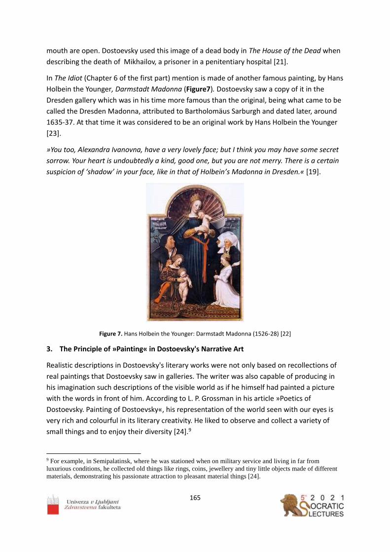
165
mouth are open. Dostoevsky used this image of a dead body in The House of the Dead when
describing the death of Mikhailov, a prisoner in a penitentiary hospital [21].
In The Idiot (Chapter 6 of the first part) mention is made of another famous painting, by Hans
Holbein the Younger, Darmstadt Madonna (Figure7). Dostoevsky saw a copy of it in the
Dresden gallery which was in his time more famous than the original, being what came to be
called the Dresden Madonna, attributed to Bartholomäus Sarburgh and dated later, around
1635‐37. At that time it was considered to be an original work by Hans Holbein the Younger
[23].
»You too, Alexandra Ivanovna, have a very lovely face; but I think you may have some secret
sorrow. Your heart is undoubtedly a kind, good one, but you are not merry. There is a certain
suspicion of ‘shadow’ in your face, like in that of Holbein’s Madonna in Dresden.« [19].
Figure 7. Hans Holbein the Younger: Darmstadt Madonna (1526‐28) [22]
3. The Principle of »Painting« in Dostoevsky's Narrative Art
Realistic descriptions in Dostoevsky's literary works were not only based on recollections of
real paintings that Dostoevsky saw in galleries. The writer was also capable of producing in
his imagination such descriptions of the visible world as if he himself had painted a picture
with the words in front of him. According to L. P. Grossman in his article »Poetics of
Dostoevsky. Painting of Dostoevsky«, his representation of the world seen with our eyes is
very rich and colourful in its literary creativity. He liked to observe and collect a variety of
small things and to enjoy their diversity [24].9
9 For example, in Semipalatinsk, where he was stationed when on military service and living in far from
luxurious conditions, he collected old things like rings, coins, jewellery and tiny little objects made of different
materials, demonstrating his passionate attraction to pleasant material things [24].

166
As Grossman says, in Dostoevsky's novels we can always sense this meticulous attention to
»painterly« details in his description of everyday life and nature, but he represents them as
consisting of »quick brush strokes«.
Grossman makes the point that representations of landscapes are few and far between in
Dostoevsky's works. In his first novel, Poor Folk, he depicts impressions and memories of the
landscape of the village of Chermashnya, where he spent his childhood. In his later works,
the descriptions of landscapes became sparser, but there are some exceptions. One, for
example, as Grossman suggests, is the view of a Siberian landscape in The House of the Dead,
or, for instance, the beautiful romantic view of a waterfall described by prince Myshkin in The
Idiot (in Chapter 5 of the first part), which resembles a painting [24]:
»There was a waterfall near us, such a lovely thin streak of water, like a thread but white and
moving. It fell from a great height, but it looked quite low, and it was half a mile away,
though it did not seem fifty paces. I loved to listen to it at night, but it was then that I became
so restless. Sometimes I went and climbed the mountain and stood there in the midst of the
tall pines, all alone in the terrible silence, with our little village in the distance, and the sky so
blue, and the sun so bright, and an old ruined castle on the mountain-side, far away. I used to
watch the line where earth and sky met, and longed to go and seek there the key of all
mysteries, thinking that I might find there a new life, perhaps some great city where life
should be grander and richer—and then it struck me that life may be grand enough even in a
prison.« [19].
As Grossman also testifies, Dostoevsky pays much attention to the physical depiction of his
heroes. The description of his last female heroine, Grushenka in The Brothers Karamazov, is
long and in sharp contrast with other descriptions of people, where he preferred not to
describe every little detail as in a photo. His descriptions reveal instantaneous impressions
and »quick brush strokes«. Grossman also notes that Dostoevsky often uses a »Rembrandt
effect«, meaning that scenes take place in the dim light of a candle [19].
Dostoevsky fully understood the basic principle of art as being a very accurate observation
and contemplation of life. His feeling, as voiced through the mouth of Prince Myshkin in The
Idiot, was: »[…] I know nothing about painting. It seems to me one only has to look, and paint
what one sees.« [19].
4. Dostoevsky and Russian Painting. Criticism of pictures at exhibitions
Dostoevsky always made a great effort to keep abreast of new trends in Russian literature
and art in general. At the exhibitions of paintings organized every year by the St Petersburg
Art Academy, he was able to see new works by the leading Russian painters. He wrote and
published two articles about these exhibitions in which he expressed his critical opinion
about the works on display.
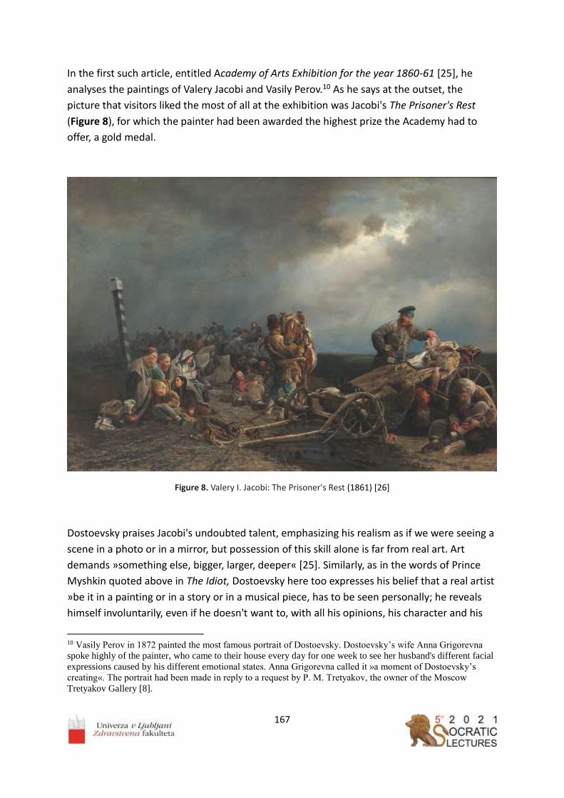
167
In the first such article, entitled Academy of Arts Exhibition for the year 1860-61 [25], he
analyses the paintings of Valery Jacobi and Vasily Perov.10 As he says at the outset, the
picture that visitors liked the most of all at the exhibition was Jacobi's The Prisoner's Rest
(Figure 8), for which the painter had been awarded the highest prize the Academy had to
offer, a gold medal.
Figure 8. Valery I. Jacobi: The Prisoner's Rest (1861) [26]
Dostoevsky praises Jacobi's undoubted talent, emphasizing his realism as if we were seeing a
scene in a photo or in a mirror, but possession of this skill alone is far from real art. Art
demands »something else, bigger, larger, deeper« [25]. Similarly, as in the words of Prince
Myshkin quoted above in The Idiot, Dostoevsky here too expresses his belief that a real artist
»be it in a painting or in a story or in a musical piece, has to be seen personally; he reveals
himself involuntarily, even if he doesn't want to, with all his opinions, his character and his
10 Vasily Perov in 1872 painted the most famous portrait of Dostoevsky. Dostoevsky’s wife Anna Grigorevna
spoke highly of the painter, who came to their house every day for one week to see her husband's different facial
expressions caused by his different emotional states. Anna Grigorevna called it »a moment of Dostoevsky’s
creating«. The portrait had been made in reply to a request by P. M. Tretyakov, the owner of the Moscow
Tretyakov Gallery [8].

168
general mindset« [25]. Further, Dostoevsky criticises some of the details depicted, doing it
with conviction and a knowledge of the subject that derive from his own personal
experience. In parallel with a story by Pliny the Elder, in which a shoemaker criticized the
shoes in a painting by the great painter of antiquity, Apelles, Dostoevsky gave reasons to
justify his critical remarks. He reproaches the painter for having painted a ring on the hand of
a deceased convict, then for having painted a thief stealing a ring; further, he claims that
other convicts would never calmly watch from the sidelines taking in the interesting scene of
an officer examining the dead man, adding that he painted shackles without leather pads
under them. Who would know better than Dostoevsky that convicts cannot possess property,
that a thief cannot steal a ring, because everyone else would like to steal such a treasure,
that all convicts would gather round to watch an officer examining a dead man, and that
shackles cannot be worn at all unless fitted with leather pads.
Similarly, writing about the exhibition in 1875, [27] he reproaches a painting by Nikolai Ge,
The Last Supper (Figure 9), which was due to be sent to the Vienna exhibition, for being too
unrealistic, embodying the high gospel theme in the guise of genre painting. Christ should be
presented not as an ordinary man, but as a God ‐ just as on Orthodox icons [27]. 11
Dostoevsky worries that in Vienna Russian painting would not be understood at all, even the
beautiful emotional, typical Russian landscapes of Arkhip Kuindzhi (Figure 10), for example,
being unlikely to strike a chord with the Germans.
11 In his journalism and letters, Dostoevsky several times expressed his opinion on the art of icon painting. In 1880,
in a letter to a collector of old icons, E. Opochinin, he stated very clearly that for him an icon is a mediator between
man and God [13].

169
Figure 9. Nikolai Ge: Last Supper (1863) [28]
Figure 10. Arkhip Kuindzhi: On a Valaam Island (1873) [29]
In 1878, at the sixth exhibition of Russian realist painters – »Peredvizhniki« (»The
Wanderers«) a painting by Ivan Kramskoj,12 The Contemplator (Figure 11), was displayed. In
The Brothers Karamazov (Chapter 6, entitled »Smerdyakov«, of the third book, first part)
Dostoevsky uses this painting to describes Smerdyakov, (the illegitimate son of Fyodor
Karamazov and lackey and assassin):
»The artist Kramskoy has one amazing painting which is called “Contemplator”: it shows the
forest in winter, and in the woods, on the road, in a ragged frock and straw shoes a lost man
is standing absolutely by himself; he is standing there as if lost in thought, but he is not really
thinking, he is “contemplating” something. If you could just push him, he would flinch and
looked at you as if just woken up but not understanding anything.« [30].
Dostoevsky sees in him a type of man, frequently encountered, who only observes, it being
impossible to guess what is hidden in the mind of this gloomy and pensive face. He could
become a saint or commit something dreadful.
12 Dostoevsky and Ivan Kramskoy (1837- 87) were friends and remained in contact for many years by
correspondence [31].

170
Figure 11. Ivan Kramskoy: The Contemplator (1876) [30]
Dostoevsky was portrayed (Figure 12) by Vasily Perov ‐ the author of genre paintings and
psychological portraits of his famous contemporaries.
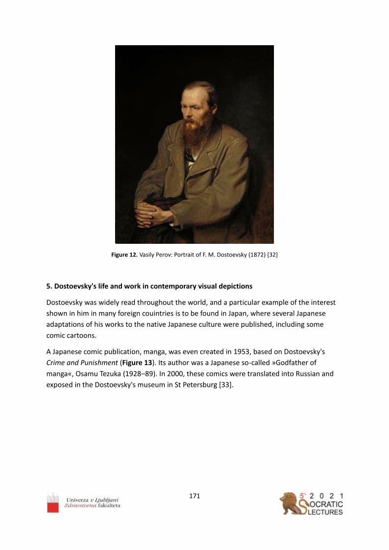
171
Figure 12. Vasily Perov: Portrait of F. M. Dostoevsky (1872) [32]
5. Dostoevsky's life and work in contemporary visual depictions
Dostoevsky was widely read throughout the world, and a particular example of the interest
shown in him in many foreign couintries is to be found in Japan, where several Japanese
adaptations of his works to the native Japanese culture were published, including some
comic cartoons.
A Japanese comic publication, manga, was even created in 1953, based on Dostoevsky's
Crime and Punishment (Figure 13). Its author was a Japanese so‐called »Godfather of
manga«, Osamu Tezuka (1928–89). In 2000, these comics were translated into Russian and
exposed in the Dostoevsky's museum in St Petersburg [33].

172
Figure 13. Osamu Tezuka: Crime and Punishment (1953) [33]
Also in America there are a few comics based on Crime and Punishment. In one of them
(from the year 2009) (Figure 14), Raskolnikov is transformed into Batman [34].
Figure 14. Dostoevsky Comics — Crime and Punishment (2009) Artist: Robert Sikoryak [34]
In February 2016, an unusual exhibition was set up in the Museum of Dostoevsky Literature
in Omsk. The artists who painted the works on display, showing portraits of Dostoevsky and
views of the old city of Omsk, were today's prisoners in Omsk, accused of serious crimes. The
exhibitions also contained models of the buildings of the forced labour camp in which
Dostoevsky was a prisoner from 1849 to 1853. This event, organized under a leitmotiv of the
famous quote from Dostoevsky's Idiot: »Beauty will save the world« celebrated the 195th
anniversary of Dostoevsky's birth and the three‐hundredth anniversary of the founding of
the city of Omsk [35].

173
References
1. Philibert, M. Dictionnaire des Mythologies. Manchecourt: Maxi – poche références.
2000.
2. Claude Lorrain. Internet source: https://en.wikipedia.org/wiki/Claude_Lorrain Accessed
on 25 April 2021.
3. Landscape with Acis and Galatea. Internet source:
https://commons.wikimedia.org/wiki/File:Claude_Lorrain_‐
_Landscape_with_Acis_and_Galatea_‐_Google_Art_Project.jpg Accessed on 25 April
2021.
4. Dostoevsky, F. Izpoved mladega človeka. Ljubljana: DZS, 1979.
5. Dostoevsky, F. Translated by S. S. Koteliansky and Virginia Woolf. Stavrogin's Confession
and The Plan of the Life of a Great Sinner. Hogarth press, Paradise Road, Richmond
1922.
6. Demons (Dostoevsky novel). Internet source:
https://en.wikipedia.org/wiki/Demons_(Dostoevsky_novel) Accessed on 27 April 2021.
7. Dostoevsky, F. The Dream of a Ridiculous Man. A Fantastic Story. Internet source:
http://www.holybooks.com/ Accessed on 18 April 2021.
8. Dostoevskaya, A. Življenje z genijem (Spomini). Kranj: Zelolepo, 2007.
9. Sistine Madonna. Internet source: https://en.wikipedia.org/wiki/Sistine_Madonna
Accessed on 25 April 2021.
10. Sistine Madonna. Internet source: http://www.raphael‐sanzio.com/sistine‐madonna/
Accessed on 25 April 2021.
11. Dostoevsky, F. 1916. The Possessed (The Devils). Translation by Constance Garnett.
Internet source: https://fb2bookfree.com/uploads/files/2020‐06/1591542278_the‐
possessed‐the‐devils‐by‐fyodor‐dostoyevsky.pdf Accessed on 22 April 2021.
12. Русский поэт Василий Жуковский о "Сикстинской Мадонне" Рафаэля 3 March
2018. Internet source: https://kinohit.mirtesen.ru/blog/43929257869/Russkiy‐poet‐
Vasiliy‐Zhukovskiy‐o‐Sikstinskoy‐Madonne‐Rafaelya Accessed on 25 April 2021.
13. Valchak, D. Д. Вальчак. «Сикстинская Мадонна», «Мертвый Христос» и икона
Богоматери: Ф. М. Достоевский о религиозной живописи и иконописи Internet
source: http://www.den‐za‐dnem.ru/page.php?article=2161 Accessed on 7 April 2021.
14. Madonna della sedia. Internet source:
https://en.wikipedia.org/wiki/Madonna_della_seggiola Accessed on 25 April 2021.
15. The Ectasy of St. Cecilia (Raphael). Internet source:
https://en.wikipedia.org/wiki/The_Ecstasy_of_St._Cecilia_(Raphael) Accessed on 25
April 2021.
16. Venere de' Medici. Internet source: https://www.uffizi.it/opere/venere‐dei‐medici
Acessed on 25 April 2021.

174
17. Stendhal syndrom. Internet source: https://en.wikipedia.org/wiki/Stendhal_syndrome
Accessed on 27 April 2021.
18. The Body of the Dead Christ in the Tomb. Internet source:
https://en.wikipedia.org/wiki/The_Body_of_the_Dead_Christ_in_the_Tomb Accesed
on 25 April 2021.
19. Dostoevsky, F. The Idiot. Freeditorial. Internet source:
https://freeditorial.com/en/books/the‐idiot‐‐5 Accessed on 22 April 2021.
20. Dostoevsky, F. The Idiot. Internet source: http://www.gutenberg.org/files/2638/2638‐
h/2638‐h.htm Accessed on 27 April 2021.
21. Dostoevsky, F. 1914. The House of the Dead or Prison Life in Siberia. Ernes Rhys Editor.
Gutenberg EBook. Internet source: https://www.gutenberg.org/files/37536/37536‐
h/37536‐h.htm#Page_194 25 September 2011. Accessed on 18 April 2021.
22. Darmstadt Madonna. Internet source:
https://en.wikipedia.org/wiki/Darmstadt_Madonna Accessed on 1st May 2021.
23. Bader, L. Artists versus art historians? Conflicting interpretations in the Holbein
controversy. Internet source:
https://arthistoriography.files.wordpress.com/2018/11/bader.pdf Accessed on 1 May
2021.
24. Grossman, L. Гроссман Л. П.: Поэтика Достоевского. Живопись Достоевского.
Internet source: http://dostoevskiy‐lit.ru/dostoevskiy/kritika/grossman‐poetika‐
dostoevskogo/grossman‐poetika‐dostoevskogo‐zhivopis.htm Accessed on 7 April 2021.
25. Dostoevsky, F. Выставка в Академии художеств за 1860‐61 год. Internet source:
http://russian‐literature.org/tom/410545 Т. 19. Статьи и заметки, 1861. Институт
русской литературы (Пушкинский Дом) Российской Академии наук.
Академические собрания сочинений. Электронная библиотека. Accessed on 18
April 2021.
26. Valery Jacobi. Internet source: https://en.wikipedia.org/wiki/Valery_Jacobi Accessed
on 25 April 2021.
27. Dostoevsky, F. Translation: Borut Kraševec. Dnevnik pisatelja 2. Izbor publicističnih
besedil. Ljubljana: Beletrina 2007.
28. Last Supper (Ge). Internet source: https://en.wikipedia.org/wiki/Last_Supper_(Ge)
Accessed on: 30 April 2021.
29. Arkhip Kuindzhi. On a Valaam Island. Internet source:
https://www.wikiart.org/en/arkhip‐kuindzhi/on‐a‐valaam‐island‐1873 Accessed on 30
April 2021.
30. Ivan Kramskoy. Contemplator. Internet source: https://todiscoverrussia.com/ivan‐
kramskoy‐contemplator/ Accessed on 1 May 2021.

175
31. Kulagina, A. Любимые картины Достоевского. Шедевры русской и мировой
живописи в творчестве писателя. Internet source:
https://diletant.media/articles/45257000/ 18 June 2019. Accessed on 1 May 2021.
32. Vasily Perov. Portrait of F. M. Dostoevsky. Internet source:
https://en.wikipedia.org/wiki/File:Vasily_Perov_‐
_%D0%9F%D0%BE%D1%80%D1%82%D1%80%D0%B5%D1%82_%D0%A4.%D0%9C.%D
0%94%D0%BE%D1%81%D1%82%D0%BE%D0%B5%D0%B2%D1%81%D0%BA%D0%BE%
D0%B3%D0%BE_‐_Google_Art_Project.jpg Accessed on 30 April 2021.
33. Японский комикс по "Преступлению и Наказанию" Достоевского. Internet source:
https://zen.yandex.ru/media/id/5ab5e8628309055286b2abf1/iaponskii‐komiks‐po‐
prestupleniiu‐i‐nakazaniiu‐dostoevskogo‐5b915e0446f39d00aa6727a5 12 September
2018. Accessed on 1 May 2021.
34. Mani Jha, A. Raskolnikov rises: Batman makes everything better. Internet source:
https://www.sundayguardianlive.com/books/387‐raskolnikov‐rises‐batman‐makes‐
everything‐better 25 July 2015. Accessed on 1 May 2021.
35. ГТРК Омск. Омские заключенные воссоздали острог времен Достоевского.
Internet source: https://www.youtube.com/watch?v=RHq8LGjQ2x0 10 February 2021.
Accessed on 18 April 2021.

176

177
___________________
The wanishing memory of the bourgeois world in Rožna dolina and Mirje
districts in Ljubljana, Slovenia
Romolo Anna1,*, Kralj-Iglič Veronika1
University of Ljubljana, Faculty of Health Sciences, Laboratory of Clinical Biophysics
Abstract
The urbane ambient reflects historical, ethnological and social status of the inhabitants.
Moreover, it exhibits the relation of those who plan the development, to the cultural
heritage. Tradition presents the link of those who presently occupy the space with those
who have lived in it before. Once destroyed, it can never be restored. Pieces of evidence
indicate that the city of Ljubljana, Slovenia has hundreds years tradition, including the
bourgeois lifestyle. Corresponding to the latter, in some districts of the city, villas embedded
in gardens can be seen, of which some are still well preserved. However, others are being
replaced by modern buildings which promote a different concept that is consistent with
higher profit of the present owners. The aim of this contribution is to observe the present
state of the villas in the district of Rožna dolina and Mirje, including those that are being
subjected to decay and eradication.
___________________

178
1. Peak of the bourgeois life in Ljubljana in the 20.th century
At the beginning of 20th century, the majority of inhabitants of Slovenia were farmers and
workers [1]. The bourgeois class was minor as regards number, however, it had a leading
role in the society. It has developed from the urban society into a privileged group, which
had an important impact on common matters. Besides outlining the values of work, money,
education and family, this class has achieved courtesy in relationships and lifestyle that
promoted well being, including all forms of culture.
Creation of an ambient is an important part of well being. The Carniola Construction Company
(founded in 1873) started building houses for the rich in Ljubljana in 1889. These objects were
constructed mostly in Vrtača, Prešernova cesta and Erjavčeva cesta [2] (Figure 1).
Figure 1. The position and the morphology of the city of Ljubljana, Slovenia. The marked areas refer to the
district with bourgeois villas and gardens. RD: the district called “Rožna dolina”, M: the district called “Mirje”.
The images were downloaded from Google Earth, June 23, 2021.
Construction was interrupted by the Ljubljana earthquake in 1995, but it continued, in
particular with the support of Ivan Hribar who became the mayor of Ljubljana in 1896. Ivan
Hribar was a polititian – a representative of Carniola within the Austro-Hungarian empire
(Carniolan Provincial Deputy, Member of the Austrian National Assembly) and after the
breakdown of the empire – the representative of Slovenia within the Monarchy Yugoslavia.
He is known for his contribution to urban development, architectural and urban renovation,
and introduction of many infrastructural innovations that meant an important step towards
a modern provincial capital and construction of a large number of nationally important
buildings. Also, he was involved in banking and investments.
Hribar was re-elected the mayor of Ljubljana several times before he was succeeded by Ivan
Tavčar. Deep involvement in investments is hinted in the memories of Ivan Hribar [3]: “Dr.
Tavčar acknowledges in the journal “Slovene nation” that someone has intervened at the
Ministry of finance aiming at exclusion of certain Ljubljana Credit Bank officers from the

179
military service; he got the answer from the person in charge: “Die Hribarbank möge
meinethalben ihre Bureaux schliesen.” Readers might have asked themselves why dr. Tavčar
has published this article that regards Ljubljana Credit Bank since it is of little interest to the
public. I think there could be many reasons such as to show a ridicule of the person in charge
at the Ministry of Finance; that the board justifies to the public why dr. Tavčar was elected
instead of me; that he himself shows the impact of war loans issued by banks; to strike me.”
And then: “He (Tavčar) had transformed the Hribar Bank - where myself founding it he at the
public meeting described as a sin - into dr. Tavčar Bank, as he made himself elected its
president.”
Hribar considered the economic, urbanistic and infrastructure point of view of the
development of the city of Ljubljana in which he involved the contribution of industrious rich
people. In urbanistic and architecture planning he connected with Maks Fabiani and Josip
Costaperaria [4,5]. Costaperaria studied architecture and art in Wienna. At first he
collaborated with Maks Fabiani. He supervised the construction of the public building
National House in Trieste designed by Fabiani in 1901-1904. Costaperaria designed a
multifunctional public pallace called Ljubljanski dvor for merchant, business, social and
residential activities and included also the cinema hall [6]. Besides being an architect of the
mayor Hribar, he collaborated with the families von Pongratz and Auersperg. He was a
member of the Rotary club Ljubljana, other societies and cultural circles. With his
modernistic views he oposed the views of then acknowledged architect Jože Plečnik.
As reviewed in [7], the district of Rožna dolina was sparsely inhabited before the earthquake,
but its development has accelerated within the reconstruction urbanization plan of Maks
Fabiani after the earthquake and continued on. Luxorious houses for the rich were built and
surrounded by large gardens. The bourgeois construction of the Rožna dolina was
concentrated mainly in the northern part along the streets Cesta na Rožnik and Večna pot. In
the green belt around the new city center, residential settlements were emerging. In Rožna
dolina, in Mirje, between Poljanska and Streliška streets, in Kodeljevo and behind Bežigrad,
most of the villas and larger single-family houses were built for wealthy citizens (Figures 2-
7). The plots were subdivided with street nets, and the newly designed neighborhoods were
mostly one-storey villas, modeled on the construction of single-family houses, outlined at
the end of the 19th century by the Vienna Cottage Verein Society. They were covered with
roofs of the prescribed slope with a predetermined layout on the land with landscaped
gardens and shaped appearance of fences, which ran exactly along the building line and
formed a closed street facade line. Thus, the appearance of the new neighborhoods was tidy
and beautiful, regardless of the diverse artistic ideas expressed on the facades. In addition to
the high quality of living, the value of the prestigious residential neighborhoods formed at
that time was also the beauty of them [7].
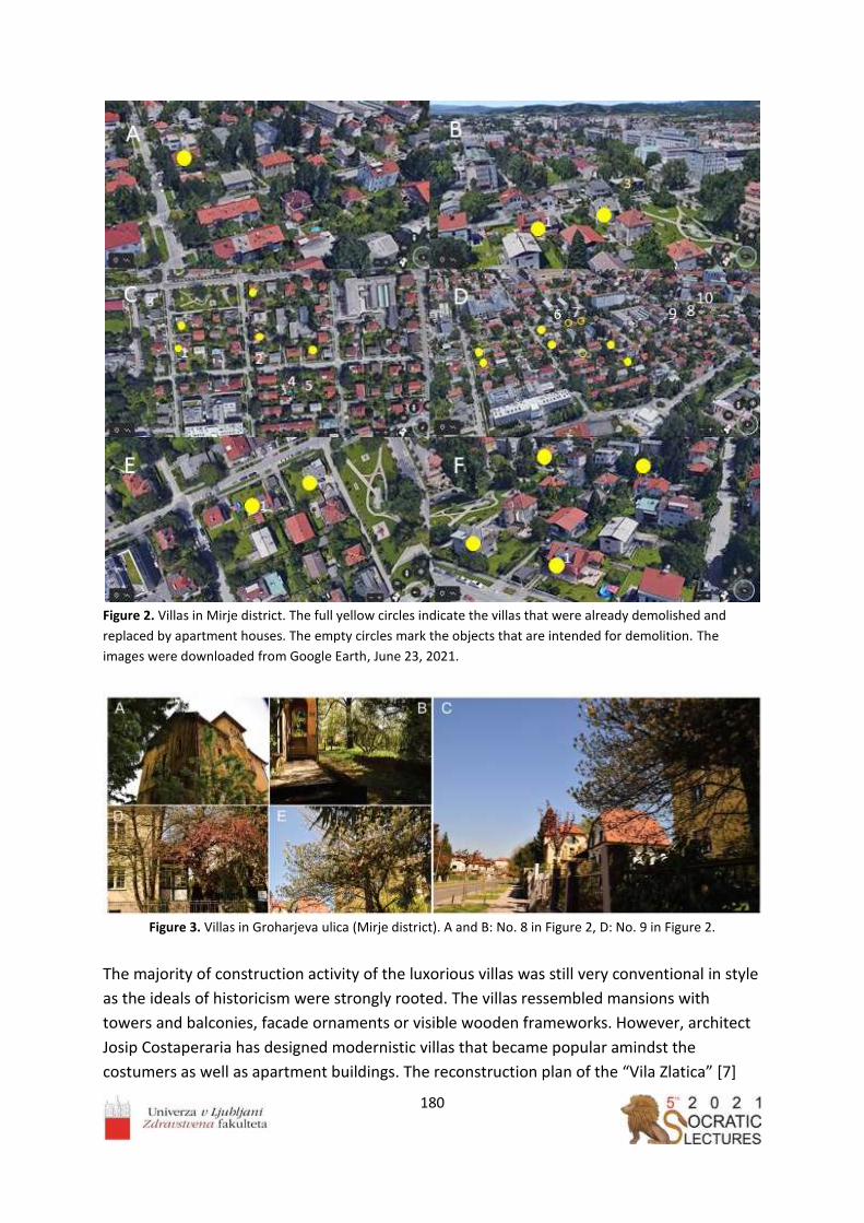
180
Figure 2. Villas in Mirje district. The full yellow circles indicate the villas that were already demolished and
replaced by apartment houses. The empty circles mark the objects that are intended for demolition. The
images were downloaded from Google Earth, June 23, 2021.
Figure 3. Villas in Groharjeva ulica (Mirje district). A and B: No. 8 in Figure 2, D: No. 9 in Figure 2.
The majority of construction activity of the luxorious villas was still very conventional in style
as the ideals of historicism were strongly rooted. The villas ressembled mansions with
towers and balconies, facade ornaments or visible wooden frameworks. However, architect
Josip Costaperaria has designed modernistic villas that became popular amindst the
costumers as well as apartment buildings. The reconstruction plan of the “Vila Zlatica” [7]

181
which belonged to Ivan Hribar’s daughter Zlatica includes detailed description of the object,
of its historical and social background and of about 3000 m2 garden which consisted of two
parts divided by the stream. Boxwood, hedges of hornbeams, various shrubs such as
currants and gooseberries, fruit trees, terracotta flowers - roses, imported from the
Netherlands tulips and daffodils, wisteria, geraniums and dahlias were grown. They had so
much fruit and berries that they also sold it (pears of various kinds, plums, apples,
strawberries, currants, raspberries), as well as hay [7].
Figure 4. A: Villas in Mirje. B: Wiew from behind the Roman wall (No. 10 in Figure 2).
Figure 5. Villas in Mirje district. A,B,D,E: Teslova ulica (A,B: No.4, D: No.5, E: No.2 in Figure 2).

182
Figure 6. Villas in Mirje district (Jamova ulica) (Nos. 3, 6 and 7 in Figure 2).
2. Dawn of the bourgeois life in Ljubljana after WW II Jealousy and hatred for the privileged ones have played an important role in features leading
to WW I and II. As things have turned out in Yugoslavia which was at the time after WW 2
the official state at the territory of Ljubljana, bourgeoisie was not in favor of the party in
power. The social middle class that originated from cities has been viewed as an idle class
which owes its well being to the exploited workers and farmers. By the laws from 1946, all
private enterprises have been nationalized [8]. In 1958, the Yugoslav state, established after
World War II, launched the third nationalisation campaign for nationalization of construction
land and residential and commercial buildings. The law indicated the compensation to the
owners, but it was not always performed. Jewish capital in Slovenia was already subject to
confiscation under German and Italian occupation in WW II, and this continued also after the
war on the basis of proclaiming them enemies due to their German origin. The villa at
Levstikova 31 was owned by Feliks and Klara Moskovič who were taken to the Auschwitz
extermination camp where they and their daughter died [9]. Their son died as an Italian
partisan [9]. The late Felix Moskovič was accused by the Yugoslav communist authorities of
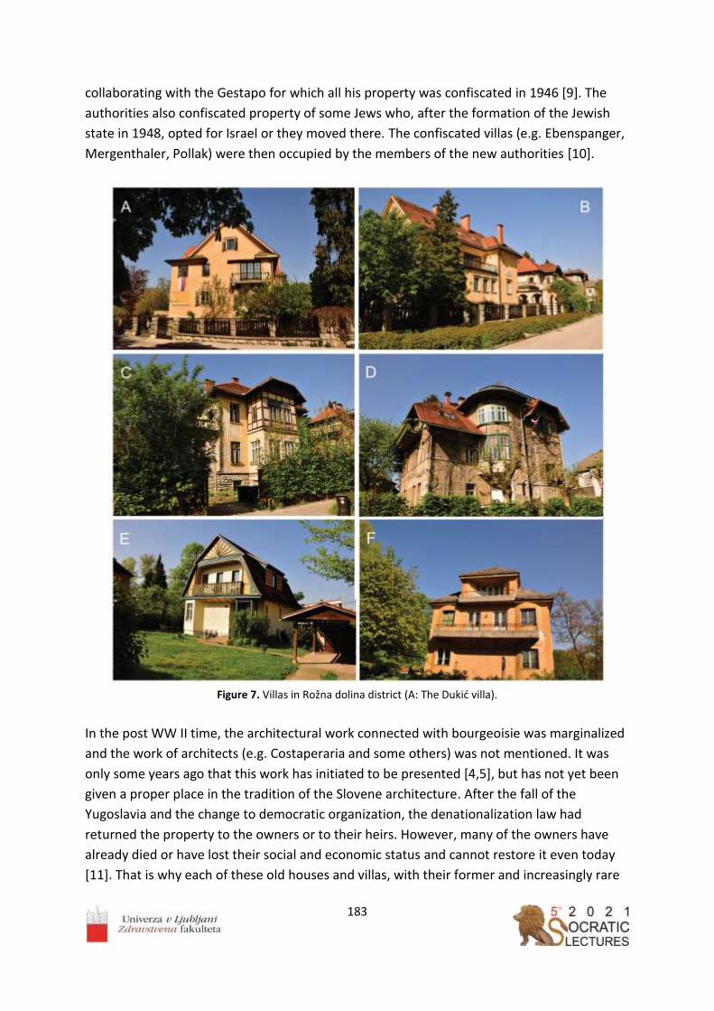
183
collaborating with the Gestapo for which all his property was confiscated in 1946 [9]. The
authorities also confiscated property of some Jews who, after the formation of the Jewish
state in 1948, opted for Israel or they moved there. The confiscated villas (e.g. Ebenspanger,
Mergenthaler, Pollak) were then occupied by the members of the new authorities [10].
Figure 7. Villas in Rožna dolina district (A: The Dukić villa).
In the post WW II time, the architectural work connected with bourgeoisie was marginalized
and the work of architects (e.g. Costaperaria and some others) was not mentioned. It was
only some years ago that this work has initiated to be presented [4,5], but has not yet been
given a proper place in the tradition of the Slovene architecture. After the fall of the
Yugoslavia and the change to democratic organization, the denationalization law had
returned the property to the owners or to their heirs. However, many of the owners have
already died or have lost their social and economic status and cannot restore it even today
[11]. That is why each of these old houses and villas, with their former and increasingly rare

184
old inhabitants and together with house objects and gardens, have special testimonial and
ethnological values, values regarding health and nature protection (high biological diversity,
beneficial microclimate) and socio-economic value (contribution to the identity of the
habitants and to the beauty and history of the city) [11].
3. The seeds of decline lie in economic laws
The Slovenian writer Ivan Mrak (1906-1986) who has thoroughly and ingeniously portrayed
bourgeois life in Ljubljana in the first part of the 20. th century has described the decline of
traditional values after the WW I due to economic reasons in his book Ivan O.; the chapter
entitled: The world of new people [12]. The main character is describing his father, the
“Roman”, a wealthy innkeeper and a gentleman, facing the appearance of newly rich after
the WW I:
“In the beginning of the world war my father has bought an oversized amount of wine. I
think he invested his entire capital as much as it was available to him; he even indebted
himself. As soon as it was heard that there is going to be a war with Italy, he hastily sold the
whole supply for a quarter of the initial price. That was the first mortal blow to his property.
After the war – due to inflation – the second blow.
In a moment, he was faced with the fact that he must start anew. The man lived honorably.
The effort of his hands was blessed. And overnight, all those who were nothing just
yesterday (he did not even return their flattery greetings – not that he looked down on them
because they were poor – but because of their lowly ways) – all these have found
themselves with lots of money. Now they have houses, properties. He knows what from. The
folks know too, they whisper, but deeply greet the newly rich. He despises all that. He could
have gained in similar ways if he wanted to, but he loathes such ways. These newly rich, war
profiteers and second hand merchants sit around in his inn, course and present themselves
with bloat. The ever-drunk Dolfe whose wife has been coming in rages to my mother for the
soup, today owns a two-story house, a carriage and horses. My father does not shake hands
with any of these. He despises their pomp and screaming wealth.
The sophisticated fabrics have all been taken by servant girls and footmen. Should he teach
them the finery of vinery? Their throats are too rough. The vines that he holds in his cellar
are too subtle for this nobility. Instead, cheap wines are gaining popularity in Ljubljana. He
finds them rough and vulgar. But since they are cheap they can be bought in almost all
restaurants and inns. Who would drink the ones from Štajerska which are too expensive?
The newly rich have shown the conceited Roman his power and worth. For them wine is
wine. They find no difference and they acknowledge none. Why would a man drink the
expensive ones from Štajerska when the fashionable ones are so devilishly cheap?
The father is more and more tired every day. He retreats more and more to his chambers.
He visits guests more and more seldom. He feels that the time has overturned. He bitterly
finds that what subject to natural laws should be found at the bottom, has swam to the top.

185
That the money has overwhelmed everyone and that the idea that the man is for the money
and not the other way around, has overcome everything.”
Economical reasons seem timeless. The villas and the gardens are a potential source of
profit, in this particular at the account of eradication of houses and gardens for building
apartment houses which can occupy considerably larger area and attain considerably larger
volumes than the original ones. Laws that pose bounds to the wish for profit allow
considerable changes in the concept of building and lifestyle of the former districts of beauty
and sophistication.
When the tradition is considered, there is a question whether it is better to conserve and
restaurate or tear down and build new. There are multiple criteria to take into account:
- The condition of the building as regards its stability
- A possibility of tearing down a part of the building, complement it with a new part
and integrate the parts
- If it is necessary to tear down the building, it could be thought how to construct the
new building to fit into the existing ambient and its tradition
- Conservation of the original area of the building and of the garden
- Using the same material or parts of the building (e.g. decorations, fences) in
restauration and the same colors
The planning could take into account the possibilities that the evidences from the past are
conserved and not destroyed, as every building carries a message for the existing and future
population. It is a part of the local history as well as of the architecture [13]. By treasuring
good tradition and its conservation we express our relation to the wholistic approach to
space and past and present residents.
However, some villas have already been demolished (marked with full yellow circles in
Figure 2) or are intended to be (marked with empty yellow circles in Figure 2 and shown in
Figure 3C) [14]. Already being missed is a small but exquisite villa at Teslova 12 that was a
property of the family Šantel: amindst them, the acknowledged painters Avgusta Šantel and
her children Saša, Avgusta and Henrika. The villa was surrounded by a garden with
distinguisged flowers, in particular roses that covered the whole façade, and various fruit
trees.
References
1. Kejžar K, Družabno življenje ljubljanskih meščanov v prvi polovici 20. Stoletja kot
vsebina pri pouku družbe, Thesis. University of Ljubljana, Pedagogical Faculty,
Ljubljana, 2016
2. https://www.odprtehiseslovenije.org/fabianijeva-ljubljana-brezplacna-knjiga/
3. Ivan Hribar, Moji spomini II del. Slovenska matica 1984, pp. 247.
4. Zupančič B, Pozzetto M, Josip Costaperaria in ljubljansko moderno meščanstvo. KUD
Polis, Ljubljana, 2004.
5. Zupančič B, Usode ljubljanskih stavb in ljudi, KUD Polis, Ljubljana 2007.

186
6. Josip Costaperaria. http://sokultura.si/wp/mesto-kultur/josip-costaperaria/
7. Klančar V, Konservatorski načrt Vile Zlatica, Mestna občina Ljubljana, Ljubljana,
Slovenia.
8. https://www.kamra.si/mm-elementi/item/jugoslovanski-zakon-o-nacionalizaciji-iz-
leta-1946.html
9. https://www.casnik.si/kaksna-je-resnicna-usoda-moskoviceve-vile/
10. Podbersič R, Mestna zaplembena komisija v Ljubljani plenila lastnino Judov, Časnik,
maj 2017, https://www.casnik.si/aktualnim-polemikam-ob-rob/
11. Zorko I, Kruta usoda naselbinske dediščine prve polovice 20. Stoletja. Outsider, 2021,
https://outsider.si/ira-zorko-kruta-usoda-naselbinske-dediscine-prve-polovice-20-
stoletja/
12. Mrak I, Ivan O. Prešernova družba, 1991, pp:62-64.
13. Deu Ž, Odprta vrata: Stara vila – občutje udobja, varnosti in doma,
http://www.deloindom.si/rustikalni/odprta-vrata-stara-vila-obcutje-udobja-varnosti-
doma
Iglič A, Načrtno uničevanje slovenske meščanske stavbne dediščine v Ljubljani ter gradnja
nadomestnih betonskih kocka‐ in kvadro‐blokov, Demokracija, nov. 2020

187

188
__________________
Postural sway on inclined surfaces
Rugelj Darja*
University of Ljubljana, Faculty of Health Sciences, Biomechanical Laboratory, Slovenia *[email protected]‐lj.si
Abstract
Professional and recreational activities are often performed on inclined surfaces, which can
thus influence postural stability. The purpose of the present study was to evaluate the
influence of three different surface inclinations (7, 13 and 19 degrees, toes up) on postural
sway during quiet standing and to define the inclination that is already steep enough to
influence postural stability. The group consisted of young healthy college students, 6 males
and 15 females, with an average age of 22.5 (3.2) years. The average height and weight were
169.9 (9.5) cm and 62.6 (11.3) kg, respectively. Postural sway was measured using a force
platform, and four postural variables were selected for analysis. The results show that the
mean velocity of the center of pressure, its medio-lateral and antero-posterior path, and the
sway area increased with the increase in the angle of inclination. There was a significant
increase of the sway for the 19-degree toe up position for all sway variables evaluated (p
<0.01). These results suggest decreased postural stability when standing on an inclined
surface, which is dependent on the angle of inclination of the surface and was greatest when
participants approached the available passive range of their ankle joint motion. These results
are of importance when considering the safety of individuals working on inclined surfaces.
__________________

189
1. Introduction
The work environment in a variety of occupations requires standing on inclined slopes.
Typically roofers, lumbers and firefighters in mountainous regions. In an environment that is
challenging for postural control, there is an increased risk of losing balance and possibly
falling. Loss of balance has been reported to be the leading precipitating factor leading to a
fall in the construction work environment [1]. Injuries are the second leading cause of lost
work time in the 20-60 age group, which is the active working population (NIJZ).
In addition to work, people engage in various recreational activities that require maintaining
balance on inclined surfaces. For example, a survey of the Slovenian population found that
14.6 per cent of people in the 20-65 age group hike and climb mountains in their leisure time
[2]. Mountain climbing is also popular among individuals in advanced age groups [3]. The
most common types of injuries among recreational hiking and mountaineering include
sprains, strains and soft tissue injuries (28%), with ankle sprains being the most commonly
reported type of injury (74%)[4]. Therefore, there is a need to investigate the postural
stability issues associated with different slope inclinations and define the inclination that is
already steep enough to affect postural stability and therefore poses a potential risk for loss
of balance. When the support surface is very steep, such as 26 degrees, the kinematics of
the whole body changes to adapt to the degree of inclination of the support surface [5] and
alters postural stability. Available research reports focus on two directions of inclined
surfaces: one experimental condition with toes up and the other with toes down [6,7].
Previous reports of postural sway on inclined surfaces investigated toe elevation in the range
of 5 degrees [8], 8.5 degrees [7], 10 degrees [6], 14 degrees [9], 26 degrees [10], and up to
34 degrees [11].
Regardless of the angle of inclination of the support surface, the authors report its influence
on postural response, including postural sway. During outdoor activities, the degree of
inclination varies. Therefore, we decided to investigate the dependence of postural sway at
four different surface inclinations. However, we wanted to exclude the contribution of knee
flexion to postural sway because subjects tilt their bodies forward and flex their knees during
standing or walking [12] on very steep surfaces, which changes body kinematics. Therefore,
the surface inclinations were within the average available range of motion of ankle
dorsiflexion. The aim of the present study was to investigate the influence of four different
surface inclinations (0, 7, 13, 19 degrees, toes up) on postural sway and to define the
smallest inclination that is already steep enough to influence postural stability. We
hypothesized that the magnitude of the center of pressure (CoP) variation depends on the
angle of the surface inclination and consequently on the degree of dorsiflexion in the ankle
joint and the degree of stretching of the calf muscle.

190
2. Methods 2.1 Participants
Twenty-one healthy college students, with no known history of musculo-skeletal injury
requiring medical treatment or a neurological history, participated in this study. The average
age (± SD) of the participants was 22.5 (3.2) years. The average height and mass were 169.9
(9.5) cm and 62.6 (11.3) kg, respectively. The group consisted of 6 male and 15 female
participants. The Slovenian National Medical Ethics Committee approved the study and
participants provided written informed consent prior to participation.
2.2 Procedure
Each participant stood on a level surface and on three different surfaces with an inclination
of 7, 13 and 19 degrees, all in toe-up orientation. The inclined surfaces were realized by
wooden blocks on which the participants stood during the experiments (Figure 1). The
wooden blocks were 40 cm wide and 30 cm long, and their height at the highest point
ranged from 3.5 cm, 7 cm to 10.7 cm, thus forming inclined surfaces of 7, 13 and 19 degrees.
Participants were instructed to stand as still as possible on the wooden blocks placed on the
Kistler 9286 force platform AA (Kistler, Winthertur, Switzerland) with their feet together,
arms at their sides, and facing a point marked on the wall approximately 3 m away. The first
measurement was taken on level surface, followed by 7, 13 and 19 degrees of surface
inclination. The last, control condition, took place again on the level surface. Thus, all
participants were tested in five consecutive trials, each lasting 60 seconds. Between trials,
there was a one-minute rest in a seated position. Data were collected at a sampling rate of
50 Hz. The raw data were further analyzed using a specially developed software [13].
Figure 1. Experimental set up for postural sway measurements on an inclined surface.

191
2.3 Calculation
Data analysis was performed using web-based software developed specifically for our
stabilometric measurements [13]. Analysis of the stabilometric data began with smoothing
the recorded CoP positions in the medio-lateral and antero-posterior directions using
Gaussian averages over 3 adjacent points. Four sway parameters were chosen for this
analysis: (1) medio-lateral (2) and antero-posterior path lengths, (3) mean velocity, and (4)
the sway area. Test-retest reliability of the system was established for young and elderly
persons [14].
2.4 Statistical analysis
The Statistical Package for Social Sciences (SPSS 26, SPSS Inc., Chicago, IL USA) was used for
statistical analysis. For the stabilometric data, one-way ANOVA was calculated using LSD
(Least significant difference) post hoc test. The significance level was set at p <0.05.
3. Results The descriptive values of the group average for the four selected postural sway variables at
different inclinations are shown in Table 1. Four participants were unable to maintain their
knees in an extended position while standing on a 19 degree slope, and all of their sway
parameters deviated more than 1 and 2 standard deviations from the group average.
Therefore, the results of these participants were excluded from the analysis of the 19-degree
toe-off position. One-way repeated measures ANOVA for the selected sway parameters
showed a significant effect of surface inclination on mean velocity (F = 3.965, p = 0.005),
total medio-lateral path length (F = 2.926, p = 0.025), and total antero-posterior path length
(F = 3.505, p = 0.010), while sway area did not differ significantly between the different
surface inclinations (F = 1.521, p = 0.202). Post-hoc tests were calculated relative to the level
ground standing and showed a significant difference between the level surface and the 19
degree inclination for mean velocity (p = 0.002), total medio-lateral path length (p = 0.015),
total antero-posterior path length (p = 0.002), and sway area (p = 0.025).
Regression analysis showed a linear relationship between surface inclination and postural
sway variables:CoP mean velocity increased by 0.014 cm/s per degree of inclination (R2 =
0.87), antero-posterior path length increased by 0.38 cm per degree of inclination (R2 =
0.89), medio-lateral path length increased by 0.51 cm per degree of inclination (R2 = 0.63),
and sway area increased by 0.08 cm2 per degree (R2 = 0.99) (Figure 2).
Repeatability obtained by comparing the two no inclination conditions and an LSD post-hoc
test showed no significant differences for all sway variables at p between p = 0.652 for sway
area and p = 1 for medio-lateral sway.

192
Table 1. Average values and their standard deviations for the five variables calculated for all surface
inclinations. The significant difference compared to the level ground condition is bolted (p <0.01).
Level 7 degrees
toes-up
13 degrees
toes-up
19 degrees
toes-up
Control
Mean velocity (cm/s) 1.01 ± 0.21 1.02 ± 0.21 1.13 ± 0.28 1.27 ± 0.29 1.01 ± 0.22
ML path length(cm) 45.14 ± 9.51 46.16 ± 9.75 48.16 ± 9.21 52.53 ± 8.70 42.90 ± 8.53
AP path length (cm) 31.50 ± 8.23 41.34 ± 7.57 37.30 ± 15.38 43.27 ± 14.76 33.59 ± 9.94
Sway area (cm2) 2.99 ± 1.71 3.64 ± 2.09 3.98 ± 2.45 4.56 ± 2.52 3.36 ± 1-76
ML medio-lateral, AP antero-posterior
a b
c d
Figure 2. Medio-lateral (a) antero-posterior path length (b), mean velocity (c) and sway area (d) are plotted as a
function of the inclination of the support surface.
193
4. Discusion
In the present study, the aim was to identify the toe-up inclination at which immediate
increase of postural sway was observed. The inclined surface varied in angles from level to 7,
13, and 19 degrees toe-up. The results show a gradual increase in postural sway with
statistically significant effect of inclination on postural sway at 19 degrees toe up. These
results suggest that the degree of slope affects the magnitude of postural sway. In the
present study, small slope inclinations (7 and 14 degrees) resulted in a non-significant
increase of the CoP variables. These results are consistent with those of [9], where the
response of CoP was measured at 14 degrees toe up and no effect on postural sway was
found. Similar to our study, participants were also asked to keep their knees in an extended
position. When participants stood at 26 [11] or 25 degrees toe up [15], an increase in medio-
lateral sway was noted. Therefore, based on the current research and previous research, we
can conclude that toe up at 20 degrees of tilt results in an increased amount of postural
sway.
Our maximum inclination was chosen to require approximately the average passive range of
motion (ROM) of dorsiflexion in the ankle joint, which is 20 degrees [16]. Interestingly, we
found that even some young participants were unable to maintain their knees in an
extended position while standing on a 19 degree toe contact patch, which is consistent with
Soucie et al., (2011) [17] who later reported lower values of passive ROM (17.3 degrees for
females and 16.3 degrees for males) for a group of young individuals. Therefore, four of our
participants had to be excluded from the analysis of the 19-degree toe-off position because
they were unable to maintain a straight knee position. The study results show that
increasing the upward toe tilt towards the limits of the passive ROM of the ankle joint leads
to increased postural sway. While lesser dorsiflexion did not result in a significant incerase of
postural sway. A linear relationship was particularly pronounced for mean velocity of the
CoP (R2=0.99) and antero-posterior path length (R2=0.89). Mean velocity is one of the most
sensitive indicators of the multiple variables of postural sway [18,19] and is often used as the
main variable in stabilometric measurements.
Changes in the length and tension of muscles, tendons, and other soft tissue extensions can
temporarily alter proprioception, which may contribute to instability [20]. With prolonged
standing on inclined surfaces, the proprioceptive system adapts, such that persons who rely
primarily on proprioceptive afferent flow to establish their frame of reference tend to
maintain the forward inclined position after returning to standing on a flat support surface
[8]. Subjects exposed to 26 degrees of incline for up to 2 hours were unstable compared to
standing on a flat surface [10]. Additionally, proprioceptive systems can be negatively
affected by muscular fatigue due to the decrease in muscle function and decreased
activation of muscular mechanoreceptors [21], as fatigued muscles are unable to produce
and maintain the desired force output, and in addition, fatigue also negatively affects
proprioceptive systems. Increased inclination alone significantly increased electromiographic
activity in the tibialis anterior muscle [22]. However, ankle muscle fatigue could not be the

194
explanation for the present results, as the duration of exposure to the inclined surface was
60 seconds for each incline and a total of five minutes for each participant, with rest periods
in between. However, in recreational walking or occupational activities on inclined surfaces,
muscle fatigue may be induced by prolonged activities that are not necessarily of high
intensity. Fatigue can be induced at intensities less than 15% of maximal voluntary
contraction if the duration is sufficiently long (1 - 8 hours) [23]. With fatigue, the latency of a
response may be increased, which can adversely affect both normal and reactive emergency
control to a perturbation [24]. In addition, local ankle muscle fatigue is known to result in a
significant increase in antero-posterior sway and mean velocity [25].
Challenging environments such as rooftops, working on sloping terrain on hillsides such as
firefighters, loggers, mountain climbers, or recreational hikers walking on inclined and
uneven trails increase the risk of balance loss and potential injury. During the above
activities, the slope of the support surface can vary from slightly steep to very steep,
resulting in variable foot and ankle flexion position and muscle activity requirements. The
slope of the supporting surface of more than 20 degrees seems to be the one at which
postural stability decreases significantly. In addition to the slope of the hill, it is reasonable
to expect the combined effect on postural stability of different surface slopes along with the
effect of the additional load in the form of professional equipment or a backpack, which can
reach up to 29% of body weight [5]. The contribution of additional load carried on the back
showed a linear increase in postural instability when carrying a backpack with 12, 21 and 30
kg load [26]. Carrying an external load potentially increases the risk of falling, regardless of
age, physical fitness, or the purpose of carrying the load, be it duty or leisure.
The limitation of the present study is a relatively small number of participants and a non-
randomized order of trials with gradual increase in slope. However, the control
measurement as the final measurement confirms that the change in the magnitude of
postural sway is a result of the different slopes. Further research is needed to combine the
three risk factors for postural destabilization: surface slope, added load, and age.
In conclusion results show the increase in postural sway when participants stood on three
progressively inclined surfaces. The increase was observed at all inclinations, with postural
sway increasing the most when participants stood near the available passive range of motion
at the ankle. These results are of importance when considering the safety of individuals
working on inclined surfaces or recreational hikers of various ages.
Acknowledgements
Authors acknowledge support of ARRS, grant P3-0388.
195
References 1. Wade C, Davis J, Weimar WH, Balance and exposure to an elevated sloped surface.
Gait Posture. 2014; 39(1):599-605. doi: 10.1016/j.gaitpost.2013.09.017
2. Pori M, Sila B, S katerimi športnorekreativnimi dejavbnostmi se Slovenci najraje
ukvarjamo? Šport. 2010; LVII (1-2):105-107.
3. Pori M, Pori P, Sila B, Ali starost vpliva na izbor najbolj priljubljenih športnih
rekreativnih dejavnosti? Šport. 2010, LVII (1-2), 112-114.
4. Lobb B, Load carriage for fun. Appl Erg. 2004; 35:541-547. doi:
10.1016/j.apergo.2004.06.006
5. Dutt-Mazumder A, Challis J, Newell K, Maintenance of postural stability as a function of
tilted base of support. Human Movement Science. 2016; 48: 91-101.
doi:10.1016/j.humov.2016.04.010
6. Sasagawa S, Ushiyama J, Masani K, Kouzaki M, Kanehisa H, (). Balance control under
different passive contributions of the ankle extensiors: quiet standing on inclined
surfaces. Exp Brain Res, 2009; 196:537-544. doi:10.1007/s00221-009-1876-4
7. Garkavenko W, Gorkovenko AV, Kolosova EV, Korneyev VV, Melnichouk AV, Vasilenko
DA, Modification of stabilogram during upright standing posture under conditions of
inclines of the supporting surface. Neurophysiol. 2012; 44:132-137. doi:
10.1007/s11062-012-9279-8
8. Kluzik JO, Horak FB, Peterka RJ, Differences in preffered reference frames for postural
orientation shown by after-effects of stance on an inclined surface. Exp Brain Res.
2005; 162:474-489. doi:10.1007/s00221-004-2124-6
9. Mezzarane RA, Kohn AF, Control of upright stance over inclined surface. Experimental
Brain Research. 2007; 180:377-388. doi: 10.1007/s00221-007-0865-8
10. Wade C, Davis J, Postural sway following prolonged exposure to an inclined surface.
Saf Sci. 2009; 47:652-568. doi:10.1016/j.ssci.2008.09.002
11. Simeonov P, Hsiao H, Hendricks S, Effectiveness of vertical reference for reducing
postural instability on inclined and compliant surfaces at elevation. Applied
Ergonomics. 2009; 40:353-361. doi:10.1016/j.apergo.2008.11.007
12. Leroux A, Fung J, Barbeau H, Postural adaptation to walking on inclined surfaces: I.
Normal strategies. Gait Posture. 2002; 15:64-74. doi:10.1016/s0966-6362(01)00181-3
13. Sevšek F, Rugelj D. StabDat V 3.0. Faculty of health sciences, Ljubljana. 2020.
http://manus.zf.uni-lj.si/stabdat
14. Rugelj D, Hrastnik A, Sevšek F, Vauhnik R, Reliability of modified sensory interaction
test as measured with force platform. Med Biol Eng Comput. 2015; 53(6):525–534. doi:
10.1007/s11517-015-1259-x
15. King AC, Patton J, Dutt-Mazumder A, Newell KM, Center-of-pressure dynamics of
upright standing as a function of sloped surfaces and vision. Neurosc Letters. 2020;
737:135334. doi: 10.1016/j.neulet.2020.135334

196
16. Palmer ML, Epler ME, Clinical Assessment Procedures in Physical Therapy. New York
Philadelphia, J.B. Lippincont Co. 1990.
17. Soucie JM, Wang C, Forstyh A, Funk S, Denny M, Roach KE, Range of motion
measurements: reference values and a database for comparison studies. Haemophilia.
2011; 17:500-507. doi:10.1111/j.1365-2516.2010.02399.x
18. Raymakers JA, Samson MM, Verhaar HJJ, The assessment of body sway and the choice
of the stability parameter(s). Gait Posture. 2005; 21:48-58. doi:
10.1016/j.gaitpost.2003.11.006
19. Doyle TLA. Dugan EL, Humphries B, Newton RU, Discriminating between elderly and
young using fractal dimension analysis of centre of pressure. Int J Med Sci. 2004; 1(1):
11-20. doi:10.7150/ijms.1.11
20. Breloff SP, Wade C, Waddell DE, Lower extremity kinematics of cross-slope roof
walking. Appl Erg. 2019; 75:134-142. doi: 10.1016/j.apergo.2018.09.013
21. Vuillerme N, Forestier N, Nougier V, Attentional demands and postural sway: the effect
on the calf muscles fatigue. Med Scie Sports Exercise. 2002; 169(2):1907-1912. doi:
10.1097/00005768-200212000-00008
22. Lu ML, Kincl L , Lowe B, Succop P, Bhattacharya A, Muscular activity of lower limb
muscles associated with working on inclined surfaces. Ergonomics. 2015; 58:278-290.
doi:10.1080/00140139.2014.968634
23. Davidson BS, Madigan ML, Nussbaum MA, Effects of lumbar fatigue rate on postural
sway. Eur J Appl Physiol. 2004; 93:183-189. doi:10.1007/s00421-004-1195-1
24. Johnston RB, Howard ME, Cawley PW, Losse GM, Effect of lower extremity muscular
fatigue on motor control performance. Med Sci Sport Exercise. 1998; 30(12):1703-
1707. doi:10.1097/00005768-199812000-00008
25. Gimmon Y, Riemer R, Oddsson L, Melzer I, The effect of plantar flexor muscle fatigue
on postural control. J Electromyog Kinesiol. 2011; 21(6):922-928. doi:
10.1016/j.jelekin.2011.08.005
26. Rugelj D, Sevšek F, The effect of load mass and its placement on postural sway. Applied
Ergonomics. 2011; 42(6):860-866. doi:10.1016/j.apergo.2011.02.002

197