rural-urban migration and happiness in china · migration and on subjective well-being in...

66

67Chapter 4

Rural-Urban Migration and Happiness in China

John Knight, Emeritus Professor, Department of Economics, University of Oxford; Emeritus Fellow, St Edmund Hall, Oxford; Academic Director, Oxford Chinese Economy Programme

Ramani Gunatilaka, Director, Centre for Poverty Analysis, Colombo; Research Associate, International Centre for Ethnic Studies, Colombo

In preparing this chapter we have benefited greatly from the advice and comments of John Helliwell, Richard Layard, Martijn Hendriks, Carol Graham and Paul Frijters.

World Happiness Report 2018

1. Introduction

This chapter links the literatures on rural-urban

migration and on subjective well-being in developing

countries and is one of the few to do so. Using

microeconomic analysis (of people and households),

it poses the question: why do rural-urban migrant

households settled in urban China have an

average happiness score lower than that of rural

households? Three basic possibilities of mistaken

expectations are examined: migrants had false

expectations about their future urban conditions,

or about their future urban aspirations, or about

their future selves. Estimations and analyses,

based on a national household survey, indicate

that certain features of migrant conditions make

for unhappiness, and that their high aspirations

in relation to achievement, influenced by their

new reference groups, also make for unhappiness.

Although the possibility that migrants are not

typical cannot be ruled out, it is apparently

difficult for migrants to form unbiased expectations

about life in a new and different world. Since the

ongoing phenomenon of internal rural-urban

migration in developing countries involves many

millions of the world’s poor, it deserves more

attention from researchers and policymakers,

especially on the implications of migration for

subjective well-being.

Migration can be viewed as a decision, taken

independently by myriad rural-dwellers, to better

themselves and their families by moving to where

the jobs and facilities are. It is generally viewed

as a force for good, albeit one that poses many

challenges for society and for the state. There

are two main forms of rural-urban migration. One

is the permanent movement of entire households

to the city or town. The other is the temporary

movement of individual migrant workers, with at

least part of the household remaining in the

village. The choice is influenced by government

policies of encouragement or discouragement

and by the institutions which can impose private

costs and benefits on the workers or their house-

holds. Both forms of rural-urban migration can

take place simultaneously.

Rural-urban migration in developing countries is

the great exodus of our time. Rapid urbanisation

is taking place in Asia, Africa, Latin America and

elsewhere. Table 4.1 shows urbanisation in the

regions of the developing world over the period

1990-2015. In each region there was a sharp rise

in the urban population as a percentage of total

population. The increase in the urban population

of the developing regions as a whole was no less

than 1,535 million. China was outstanding both in

its increase in the urbanisation rate (by 30

percentage points) and in the number of people

becoming urbanised (by 463 million). China

accounted for 30% of the increase in urban

population of the developing world as a whole

over the period.

China’s urbanisation is not the same as its rural-

urban migration. Urbanisation comprises three

elements: reclassification of rural places as urban

places, natural increase of the urban population,

and rural-urban migration. However, China’s

rural-urban migration is likely to have made up

much of the rise in its urban population over this

quarter century.1

The data on migrants in China pose an interesting

and socially important puzzle. Migration theory

usually assumes that rural people migrate in

order to raise their utility, at least in the long run.

Thus, migrants who have made the transition into

urban employment and living are expected to be

happier than they would have been had they

remained at home. Yet our sample of rural-urban

migrants has an average happiness score of 2.4,

well below the average score of the rural sample

(2.7) and also below that of the urban-born

sample (2.5). Of course, initial hardship is to be

expected – and indeed it is predicted by migra-

tion models. However, our sample comprises

migrants who have established urban households

and whose average urban stay is no less than 7.5

years. So why is it that even seven and a half

years after migrating to urban areas, migrants

from rural areas are on average less happy than

they might have been had they stayed at home?

Unfortunately, there is as yet scant evidence to

measure and explain the subjective well-being of

rural-urban migrants in the developing world.

There is more literature on their objective

well-being (not only income but also other

physical measures of the quality of life). Fortu-

nately, there is more evidence on migrants and

their happiness in China, the country which, it is

commonly said, has recently experienced ‘the

greatest migration in human history’. There are

many lessons that China can offer policymakers

elsewhere in the developing world.

68

69

One of the themes explored in this chapter is

the relationship between actual and hoped-for

achievement, i.e. between what people manage

to achieve and what they aspire to achieve.

Reported happiness might be determined by the

extent to which aspirations are fulfilled. That

raises research questions to be explored. How

best can aspirations be measured? For instance,

are the aspirations of migrants moulded by the

achievements of the people with whom they

make comparisons? Rising aspirations in their

new environment might provide an explanation

for the relatively low happiness of rural-urban

migrants.

2. Rural-Urban Migration in China

The phenomenon of rural-urban migration has

been different in China from that in most other

poor countries.2 During its early years in power

the Communist Party separated China into two

distinct compartments – creating an ‘invisible

Great Wall’ between rural and urban China -

primarily as a means of social control. Integral

to this separation was a universal system of

household registration, known as hukou, which

accorded rights, duties and barriers. Rural-born

people held rural hukous, urban-born people

(including migrants from other urban areas) held

urban hukous, and (with a few exceptions such

as university graduates from rural areas) rural-

urban migrants retained their rural hukous. By the

late 1950s, a combination of hukou registration,

the formation of the communes, and urban food

rationing had given the state the administrative

levers to prevent rural-urban migration. Throughout

Table 4.1: Urbanisation in Developing Countries: China, Regions, and Total, 1990 and 2015

1990 2015Change

1990-2015

China

Urbanisation rate (%) 26 56 30

Urban population (millions) 300 763 463

Other East Asia and Pacific



Latin America and the Caribbean



Middle East and North Africa



South Asia



Sub-Saharan Africa



All Developing Country Regions



Notes: Derived from World Bank, World Development Indicators 2017, Online Tables, Table 3.12


the period of central planning the movement

of people, and especially movement from the

communes to the cities, was strictly controlled

and restricted.

Even after economic reform began in 1978,

migration was very limited although temporary

migration was permitted when urban demand

for labour exceeded the resident supply. The

hardships and disadvantages facing temporary

migrants holding rural hukous caused many to

prefer local non-farm jobs whenever they were

available.3 When, increasingly, migrants holding

rural hukous began to settle in the cities with

their families, they faced discrimination in access

to jobs, housing, education and health care. City

governments favoured their own residents, and

rural-urban migrants were generally treated as

second class citizens.4 For instance, they were

allowed only into the least attractive or remuner-

ative jobs that urban hukou residents shunned;

many entered self-employment, which was less

regulated. Although the urban labour markets

for urban-hukou and rural-hukou workers have

become less segmented over time, the degree of

competition between them remained very limited

in 2002.5 The tough conditions experienced by

rural-urban migrants living in urban China might

provide another explanation for their lower

happiness.

Despite these drawbacks, rural-urban migration

has burgeoned as the controls on movement

have been eased and the demand for urban

labour has increased. A study drawing on official

figures, reported that the stock of rural-urban

migrant workers was 62 million in 1993 and 165

million in 2014, in which year it represented 43%

of the urban labour force.6 An extrapolation from

the 2005 National Ten Percent Population Survey

on the basis of forecast urban hukou working

age population and of assumed urban employment

growth derived a stock of rural-hukou migrant

workers in the cities of 225 million in 2015,

having been 125 million in 2005.7 Despite the

difficulties of concept, definition and measurement

(which no doubt explain much of the difference

between the estimates for 2014 and 2015), it is

very likely the case that China is indeed experi-

encing ‘the greatest migration in human history’.

Although a large percentage of migrants come

temporarily to the cities with the intention of

returning home, an increasing percentage wish

to settle in the cities, and are establishing urban

households. As Figure 4.1 below suggests, and

as evidence of migrant wages in urban China

confirms8, the prospect of income gain was the

likely spur to the great migration.

3. Overview of Rural-Urban Migration in China

This study is based on an urban sample of rural-

urban migrant households collected as part of a

national household-based survey.9 The survey was

conducted by the National Bureau of Statistics

early in 2003 and its information generally relates

to 2002. There was no repeat interviewing of the

same households although there were some

questions that required recall of the past or projec-

tion of the future. The urban and rural samples were

sub-samples of the official annual national house-

hold survey. However, because the official urban

survey covered only households possessing urban

hukous and did not yet cover households possessing

rural hukous, the rural-urban migrant sample was

based on a sampling of households living in

migrant neighbourhoods in the selected cities.

Migrants living on their own temporarily in the

city before returning to the village were excluded.

The migrant survey contains a great deal of

information about the household and each of

its members, including income, consumption,

assets, housing, employment, labour market

history, health, education, and rural links. Less

commonly, various migrant attitudes and

perceptions were explored. The great advantage

of this survey is that the separate questionnaire

module on subjective well-being contained

specially designed questions that help to answer

the questions posed in this chapter.

The question on subjective well-being that was

asked of one of the adults in each sampled

household was: “Generally speaking, how happy

do you feel nowadays”? The six possible answers

were: very happy, happy, so-so, not happy, not at

all happy, and don’t know. They were converted

into cardinal scores as very happy = 4, happy = 3,

so-so = 2, not happy = 1, and not at all happy = 0;

the small number of don’t knows were not used

for the analysis. The happiness variable is critical

for our analysis as it is the dependent variable in

the happiness functions that are estimated to

explain happiness.

70

71

It is helpful first to provide descriptive informa-

tion about the migrants before presenting the

happiness functions that will explain what makes

rural-urban migrants happy or unhappy. This

will inform our interpretations. Consider the

characteristics of those household members

– 77% of whom were the household head - who

responded to the attitudinal questions: 61% were

men, 90% were married, 93% were employed,

and 88% were living with their family. These

respondents were generally not pessimistic

about the future: 7% expected a big increase in

real income over the next five years, 55% a small

increase, 28% no change, and only 10% a de-

crease. Rural links were commonly retained: 53%

had family members who still farmed in the village,

51% remitted income to the village, and 32% had

one or more children still living in the village.

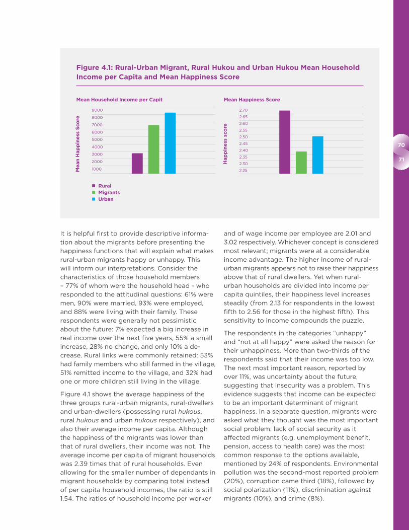
Figure 4.1 shows the average happiness of the

three groups rural-urban migrants, rural-dwellers

and urban-dwellers (possessing rural hukous,

rural hukous and urban hukous respectively), and

also their average income per capita. Although

the happiness of the migrants was lower than

that of rural dwellers, their income was not. The

average income per capita of migrant households

was 2.39 times that of rural households. Even

allowing for the smaller number of dependants in

migrant households by comparing total instead

of per capita household incomes, the ratio is still

1.54. The ratios of household income per worker

and of wage income per employee are 2.01 and

3.02 respectively. Whichever concept is considered

most relevant; migrants were at a considerable

income advantage. The higher income of rural-

urban migrants appears not to raise their happiness

above that of rural dwellers. Yet when rural-

urban households are divided into income per

capita quintiles, their happiness level increases

steadily (from 2.13 for respondents in the lowest

fifth to 2.56 for those in the highest fifth). This

sensitivity to income compounds the puzzle.

The respondents in the categories “unhappy”

and “not at all happy” were asked the reason for

their unhappiness. More than two-thirds of the

respondents said that their income was too low.

The next most important reason, reported by

over 11%, was uncertainty about the future,

suggesting that insecurity was a problem. This

evidence suggests that income can be expected

to be an important determinant of migrant

happiness. In a separate question, migrants were

asked what they thought was the most important

social problem: lack of social security as it

affected migrants (e.g. unemployment benefit,

pension, access to health care) was the most

common response to the options available,

mentioned by 24% of respondents. Environmental

pollution was the second-most reported problem

(20%), corruption came third (18%), followed by

social polarization (11%), discrimination against

migrants (10%), and crime (8%).

Figure 4.1: Rural-Urban Migrant, Rural Hukou and Urban Hukou Mean Household Income per Capita and Mean Happiness Score

Mean Household Income per Capit Mean Happiness Score

2.70

2.65

2.60

2.55

2.50

2.45

2.40

2.35

2.30

2.25

9000

8000

7000

6000

5000

4000

3000

2000

1000

Me

an

Hap

pin

ess

Sco

re

Hap

pin

ess

sco

re

Rural Migrants Urban


Migrants were also asked: “Compared with your

experience of living in the rural areas, are you

happier living in the city”? No fewer than 56% felt

that urban living gave them greater happiness,

41% reported themselves equally happy in rural

and urban life, while only 3% reported greater

rural happiness. When asked what they would do

if forced to leave the city, more migrants would

go to another city (54%) than would go back to

their village (39%). These results add to the

puzzle. If most migrants view urban living as

yielding them greater happiness, and most wish

to remain in an urban area, why are their mean

happiness scores lower than those of rural

residents?

4. Possible Explanations

There are several possible explanations for these

results. The first possibility is that migrants, when

they decided to migrate from the village, had

excessively high expectations of the conditions

that they would experience in the city. We shall

look for evidence that this might be the case by

considering the characteristics of their urban life

that reduce their welfare.

Second, the puzzle might be solved by recourse

to the possibility of adaptation, following Easterlin’s

evidence.10 He argues that happiness depends

both on income and aspirations, the former

having a positive and the latter a negative effect.

Moreover, as income rises over time, aspirations

adapt to income, so giving rise to what has been

called a ‘hedonic treadmill’.11 When respondents

are asked to assess how happy they had been in

the past, when their income was lower, they tend

to judge that situation by their current aspirations

for income and therefore to report that they are

more happy now. Similarly, when they are asked

to assess their happiness in the future, when they

expect to have higher income, they do not realise

that their aspirations will rise along with their

income and therefore report that they will be

happier. This is possibly because, as findings

from social psychology suggest, ‘We don’t always

predict our own future preferences, nor even

accurately assess our experienced well-being

from past choices’.12

If current judgements about subjective well-

being, whether in the past, the present, or the

future, are based only on aspirations in the

present, this might explain why migrants on

average are less happy than rural people:

aspirations could have risen after having made

the decision to migrate. While aspirations might

not be directly measurable, the implications of

adaptation can be tested. Similarly, we might also

find an explanation for why it is that migrants

generally report that their happiness is higher, or

at least no lower, in urban than in rural areas.

A second possibility is that people form their

aspirations relative to some ‘reference group’, i.e.

the people with whom they compare themselves.

The reference group can change when they

move to the city and find themselves with richer

neighbours. The notion that aspirations depend

on income relative to that of the relevant reference

group comes from the sociological literature,13

and has been developed for China in related

papers on subjective well-being.14 The literature

on relative income was well summarised and

evaluated in 2008,15 since when many more

studies of the effects of relative income have been

made, albeit mainly for developed economies.

Other studies for developing countries which

show the importance of reference groups include

shifts in reference norms in Peru and Russia,16

comparison with close neighbours in South

Africa,17 and rural-urban migrants retaining a

village reference group in Nepal.18 If the group

with which the migrants compare themselves

changes as a result of rural-urban migration

and urban settlement, this might explain why

their aspirations change. We can test whether

migrants show ‘relative deprivation’ in relation

to urban society.

Our third possibility is that the presence of

members left behind in the village can place a

burden on the urban members of the two-location

family. Insofar as migrants remit part of their

income, their own happiness score might fall and

that of their rural family rise. Equivalently, our

measure of the income per capita of the urban

migrant household might overstate its disposable

income per capita.

Fourth, our results might be explained by the

untypical nature of the migrants. The lower

happiness of migrants may be the result of their,

or of their households, having characteristics

different from those of the rural population as a

whole. If this were the case, they could indeed

have been less happy on average had they

72

73

remained in the village. Such happiness-reducing

characteristics might be captured by the survey

data – and thus be capable of being accounted

for in the statistical estimations - or they might

be unobservable to the researcher. For instance,

it is possible that those rural-dwellers who by

nature are melancholy or have high and unfulfilled

aspirations hold their rural life to be responsible

and expect that migration will provide a cure.

They might therefore be more prone to leave the

village for the city. If the self-selected migrants

are intrinsically less happy, this might explain

why the sample of rural-urban migrants has a

lower average happiness score than does the

sample representative of the rural population of

which they were previously a part. Self-selection

of this sort might also involve false expectations,

in this case based on self-misdiagnosis. Its

implications can be tested.

5. The Determinants of Happiness

Happiness functions were estimated to discover

the factors associated with the happiness of

rural-urban migrants19 so as to test the possible

explanations 1, 2 and 3, just outlined. We proceed

in stages: first, we estimate ordinary least

squares (OLS) estimates of the happiness score

with a full set of explanatory variables. Second,

we investigate whether these explanatory variables

have different effects on happiness depending

on the length of time that the household had

been living in urban areas by dividing the migrant

sample into ‘short-stayers’ and ‘long-stayers’, i.e.

those who had settled in the city for less and more

than the median time (7.5 years) respectively.

Third, we confine the sample to employed

migrants, as this enables us to see whether

working conditions, denoted by work-related

variables, have an impact on happiness. However,

because the full results are available elsewhere

(Knight and Gunatilaka, 2009, 2012, on which

this chapter draws heavily) we report only the

variables that are critical for our story.

Table 4.2 reports, for the full sample but with only

the most relevant variables shown, the average

values of the explanatory variables (column 1)

and then coefficients in the happiness function

estimated with the full set of available explanatory

variables (column 2). With the happiness score

as the dependent variable (the variable to be

explained) and various independent variables

(chosen as the explanatory variables), the

estimated ‘coefficients’ on the explanatory

variables indicate the effect on happiness made

by a unit change in each explanatory variable,

holding all other explanatory variables constant.

The asterisks show levels of statistical significance:

the more asterisks against a coefficient, the more

statistically significant is the effect on happiness.

In column 2, the coefficient on log of income per

capita is significantly positive, and its value

(0.20) indicates that a doubling of income raises

the happiness score by about 0.14 points. Income

is relevant, as predicted, but its effect does not

appear powerful by comparison with either the

presumptions of economists or the estimated

effects of some other variables. For example,

reporting to be in good health (rather than not in

good health) raises the happiness score by 0.12

points according to column 2.

Migrants can be expected to adjust over time to

urban life in various ways. On the one hand, as

they overcome initial difficulties and become

more settled, we expect their happiness to rise.

On the other hand, their reference groups might

change, from the poorer, village society to the

richer, urban society, and this fall in perceived

comparative status might reduce happiness. The

length of time spent in the urban area is introduced

as an explanatory variable, and also its square so

as to allow the possibility that the relationship is

curved rather than being a straight line. The

variable and its square are both significant, the

former positively and the latter negatively

although only at the 10% critical level. The

coefficients imply that the happiness score rises

to a peak after 12 years and then declines.

However, it is possible that there is selective

settlement: happier migrants are more likely to

choose to stay long in the city. This would tend to

bias upwards the estimated returns to duration of

urban residence. In summary, it would appear

that migrants’ happiness tends to rise over several

years of urban living, but the evidence is weak.

In order to pursue the notion that reference

groups can be important, the effect of relative

income was investigated. Drawing on the urban

and rural samples of the 2002 national house-

hold survey, the average urban income per capita

in the destination city and (lacking information

on the origin county) the average rural income

per capita in the origin province of the migrant,

are introduced. The expectation is that both have


a negative coefficient, reflecting relative

deprivation. The coefficient on destination

income is indeed large and negative but not

significantly so; that on origin income is small

and positive and not significantly different from

zero. If the migrant is living with family, or has

relatives in the city who can be turned to for

help, the effect on happiness is positive, but

not significantly so in the former case. Having

a child still in the village has a significant

depressing impact. Of the housing variables,

only lack of heating is significant: the effect is

predictably negative.

Columns 3 and 4 of Table 4.2 reproduce the

equation for two sub-samples: those who had

less than 7.5 years of urban residence and those

who had more, respectively. Only the notable

variables for which there is a significant difference

in coefficients are mentioned. The long-stayers

have a higher coefficient on the income variable

(0.25 compared with 0.12). This might be because,

through self-selection, they are more successful

and happier than the short-stayers. However, the

result is also consistent with migrants learning to

enjoy the costly pleasures of urban life and so

becoming more materialistic as they get more

involved in urban society. The long-stayers are

Table 4.2: Happiness Functions of Rural-Urban Migrants: OLS Estimation

Mean or

proportion Full sampleBelow median

durationAbove median

duration

(1) (2) (3) (4)

Log of per capita household income

8.55 0.2081*** 0.1295*** 0.2766***

Duration of urban residence (years)

7.51 0.0136*

Duration of urban residence, squared

84.83 -0.0005*

In good health 0.90 0.1231** 0.0266 0.1691**

Expect big increase in income over next 5 years

0.07 0.2984*** 0.2673** 0.3373**

Expect small increase in income over next 5 years

0.55 0.0262 0.0508 -0.0035

Expect decrease in income over next 5 years

0.10 -0.4033*** -0.3221** -0.4506***

Log of average per capita income in city of current residence

8.97 -0.1204 0.0053 -0.2800**

Log of average rural income in province of origin

7.81 0.0700 0.1245 0.0519

Living with family members 0.88 0.1347 0.2079** 0.1283

Number of relatives and friends in city

7.19 0.0039* 0.0076 0.0016

Child still in village 0.32 -0.1250** -0.1254** -0.1131

No heating 0.65 -0.1499** -0.2042*** -0.1166*

Constant 1.0248 0.4658 1.6702

R-squared 0.100 0.091 0.134

Number of observations 1850 925 926

Notes: Dependent variable in this table and in Table 4.4: Score of happiness based on cardinal values assigned to qualitative assessments as follows: very happy=4; happy=3; so-so=2; not happy=1 and not at all happy=0.Model 1 is for the full sample. Models 2 and 3 are based on sub-samples selected according to the length of stay in urban areas. The omitted categories in the dummy variable analyses are: single female; employed or labour force non-participant not healthy; in normal or worse than normal mood; change in income expected in the next five years. In this and subsequent tables, ***, **, and * denote statistical significance at the one per cent, five per cent and ten per cent levels respectively. The models have been clustered at city level for robust standard errors.

74

75

more sensitive to average urban income per

capita in the destination city (a significant -0.28

compared with a non-significant -0.01). This

suggests that over time urban residents increas-

ingly become the reference group for migrants.

Moreover, the fact that this makes them relatively

less happy might explain why additional income

becomes more important for their happiness.

The sensitivity of happiness to relative income in

the destination city, especially for long-stayers,

seems to agree with our second possible

explanation, i.e. that migrants’ aspirations rise as

they adjust to their new urban environment. The

extreme sensitivity of migrant happiness scores

to income rank in the city (shown in Table 4.5

below) provides further supporting evidence.

These results were found to be unchanged using

alternative versions of the happiness variable20.

An attempt was also made to examine the

sensitivity of our results to the influence of the

unobserved determinants of happiness.21 For

instance, unobserved characteristics such as

personal energy might raise both income and

happiness, or happiness itself might improve

motivation and so raise income. The income

variable was therefore adjusted to correct for

such unobserved influences, but the results of

this exercise did not alter our story.22

We investigated the effect of working

conditions on the subjective well-being of

employed respondents. In other words, does

the unpleasantness and insecurity of urban work

contribute to the unhappiness of migrants?

Table 4.3 is based on estimates of the full sample

equation of Table 4.2 but for employed respondents

only, the reason being that it is then possible to

add various employment-related explanatory

variables.23 The first column provides mean

values and the second shows only the results for

the additional variables as the coefficients of the

variables in common barely change.

Where satisfaction with the current job is rated 4

for ‘very satisfied’ down to 0 for ‘not at all

satisfied’, this variable has the expected positive

and significant coefficient. Respondents were

asked whether rural workers enjoyed the same

treatment as urban workers in seven different

aspects of the employment relationship. The

negative answers were added to form an index

of discrimination (ranging from 0 to 7). The

coefficient is negative and significant, indicating

that perceptions of discrimination contribute

to unhappiness. Compared with being self-

employed, having permanent work or long term

contract work raises happiness but this result is

not statistically significant, i.e. it could arise by

Table 4.3: Happiness Functions of Employed Rural-Urban Migrants: OLS Estimation

Mean or proportion Coefficient

Satisfaction with job 1.98 0.0735*

Index of discrimination 5.35 -0.0322***

Permanent or long-term contract work 0.05 0.1338

Temporary work 0.24 0.0079

Can find another job in two weeks 0.11 -0.0997

Can find another job in a month 0.23 -0.1213**

Can find another job in 2 months 0.10 -0.1478*

Can find another job in 6 months 0.13 -0.1917**

Need more than 6 months to find another job 0.17 -0.2140***

R-squared 0.129

N 1715

Notes: With the addition of employment-related variables, the specification of column 2 is identical to that of column 2 of Table 4.3, but the variables presented in Table 4.3 are not reported. The omitted categories in the dummy variable analyses reported are: self-employed; can find a job immediately. The equation has been clustered at city level for robust standard errors.


chance. Another aspect of the insecurity of

urban employment can also be incorporated.

Respondents were asked how long it would take

them to find another job with equivalent pay if

they lost their current job. Compared with ‘within

one week’ - the reference category with which

other categories are compared - the coefficients

are generally significantly negative and increase

steadily in size. The evidence is consistent with

our first possible explanation: migrant employ-

ment can be unpleasant and insecure, and this

depresses migrant happiness.

The third possible explanation emerges from

theories of rural-urban migration expressed in

terms of decision-making by the rural family, of

which the migrant remains a part. The inference

is that the average happiness score of migrants

is low because they support their rural family

members by remitting part of their income to

them. In that case, our dependent variable

cannot reflect the full gain in happiness of the

two-location family. In principle the argument is

weak. First, it is less plausible for settled than for

temporary migrants. Second, ‘utility-maximising

economic agents’ (a concept commonly used by

economists!) are assumed to allocate their

income optimally, i.e. at the margin gifts yield

as much utility for the giver as consumption.

Altruism and satisfaction that they are fulfilling

their family obligations might raise migrants’

happiness. So happiness need not fall if income

is remitted. It is nevertheless true that migrant

household disposable income per capita is often

reduced by the presence of family members

elsewhere.

It is relevant that 51% of migrant households made

remittances, and that remittances represented 9%

of household income for the sample as a whole

and 17% for the remitting households. Do

remittances reduce the happiness of respondents

in migrant urban households, and so contribute

to the low average happiness score? If that were

the case, the variable log of household remittance

per capita would be significantly negative in the

estimated happiness function.24 However, whether

this term is added to the full estimated equation

or the sub-sample of remitters, the coefficient on

the remittance variable remains no different from

zero. To illustrate, when the variable log remittances

per capita is added to column 2 of Table 4.2

(not shown), the coefficient is a non-significant

0.0064. Thus, we found no evidence in support

of the third possible explanation, i.e. that migrants’

happiness is reduced because they remit part of

their income,

6. Why Are Migrants Less Happy Than either Rural Dwellers or Urban Dwellers?

Migrants might be less happy on average than

either rural or urban people because they differ

in their average characteristics, i.e. average

endowments of happiness-affecting attributes

such as health status. Here a different testing

methodology is required. The migrants are

compared with both rural and urban residents,

employing a standard decomposition technique.

The objective is to pinpoint the reasons for the

difference in happiness. The decomposition

shows the contribution to the difference in

happiness that is made by each determinant

of happiness.

We began by conducting a decomposition

analysis of the difference in household mean

income per capita, in order to throw some light

on the representativeness and the motivation of

the migrants. The decomposition methodology is

explained in the technical box below, where it is

illustrated in terms of differences in average

happiness. Those migrating from rural China are

indeed a selective and unrepresentative group.

Migrant households, had they remained in the

rural areas, would on average earn 10% less

income than do rural resident households. There

is also a considerable income advantage to their

migration: the average income that migrant

households actually earn is 2.64 times what they

would earn in the rural areas. By contrast, if they

were to migrate, average rural households would

earn 2.19 times more than they actually earn. It

appears that rural households possess productive

characteristics that are relatively valuable in the

countryside whereas migrant households possess

productive characteristics that are relatively

valuable in the city.

The average happiness score of rural people

was 2.68 and that of migrants 2.37, implying a

migrant shortfall of 0.31. Table 4.4 decomposes

this gap into the parts which can be explained

by differences between the two groups in the

average values of their characteristics and

by differences in the coefficients in the two

76

77

happiness functions. The figures show the

percentage contributions of the difference in

average values of characteristics and of the

difference in coefficients respectively.

We see from the first column of Table 4.4 that

the share of the difference in average happiness

scores that is attributable to differences in

average characteristics sums to -35%, and from

the second column that the share attributable

to differences in coefficients sums to 135%. The

effect of characteristics is therefore actually to

increase the difference in mean happiness scores.

This is mainly due to the variable log of income

per capita: the effects of income are the same

in the two samples but migrants have higher

incomes. The reason why migrants have lower

average happiness must therefore be found in

the different explanations for the happiness of

the rural and urban residents, based on their

different coefficients. The constant term, health,

and income expectations are the main

contributors, and age is the big exception.

The importance of the constant term implies

that there are unobserved characteristics that

we have not been able to include in the model

which reduce migrant relative to rural happiness.

For example, we are unable to standardise for

the various social disadvantages that migrants

encounter in the cities because the same

variables are not available in the rural data set.

Perhaps because rural people are on average

less healthy than migrants - poor health being

a deterrent to migration - they place a higher

value on good health.

In both samples happiness is highly sensitive to

expectations about future income in five years’

time. It appears from Figure 4.2 that expectations

of future income can influence current happiness.

With the expectation of no change in income as

the reference category in the dummy variable

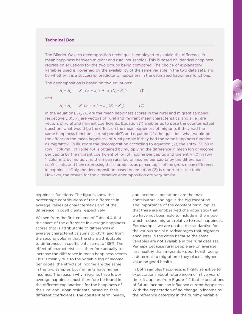
Technical Box

The Blinder-Oaxaca decomposition technique is employed to explain the difference in

mean happiness between migrant and rural households. This is based on identical happiness

regression equations for the two groups being compared. The choice of explanatory

variables used is governed by the availability of the same variable in the two data sets, and

by whether it is a successful predictor of happiness in the estimated happiness functions.

The decomposition is based on two equations:

Hr – H

m = X

m (a

r – a

m) + a

r (X

r – X

m), (1)

and

Hr – H

m = X

r (a

r – a

m) + a

m (X

r – X

m). (2)

In the equations, Hr, H

m are the mean happiness scores in the rural and migrant samples

respectively, Xr, X

m are vectors of rural and migrant mean characteristics, and a

r, a

m are

vectors of rural and migrant coefficients. Equation (1) enables us to pose the counterfactual

question ‘what would be the effect on the mean happiness of migrants if they had the

same happiness function as rural people?’, and equation (2) the question ‘what would be

the effect on the mean happiness of rural people if they had the same happiness function

as migrants?’ To illustrate the decomposition according to equation (2), the entry -55.39 in

row 1, column 1 of Table 4.4 is obtained by multiplying the difference in mean log of income

per capita by the migrant coefficient of log of income per capita, and the entry 1.01 in row

1, column 2 by multiplying the mean rural log of income per capita by the difference in

coefficients, and then expressing these products as percentages of the gross mean difference

in happiness. Only the decomposition based on equation (2) is reported in the table.

However, the results for the alternative decomposition are very similar.


analysis, the coefficients in the migrant sample

vary from 0.31, if a large increase is expected, to

0.05, if a small increase is expected, and to -0.39,

if a decrease is expected; the corresponding

estimates for the rural sample are 0.41, 0.19 and

-0.19 respectively. The fact that in the migrant

sample the coefficients are uniformly lower, in

relation to the expectation of static income,

suggests that migrants have higher aspirations

relative to their current income. This can be

expected if aspirations depend on the income of

the relevant comparator group. Whereas the

Table 4.4: Decomposition of the Difference in Mean Happiness Score between Rural-Urban Migrants and Rural Residents: Percentage Contribution to the Difference

Using the migrants’ happiness function

Due to characteristics Due to coefficients

Log of income per capita -55.39 1.01

Health -5.81 94.41

Income expectations 11.34 36.36

Age 6.69 -131.54

Other variables 7.95 5.48

Sum (percentage) -35.23 135.23

Sum (score) -0.1078 0.4137

Notes: The mean happiness scores are 2.6764 in the case of rural residents and 2.3703 in the case of migrants, creating a migrant shortfall of 0.3061 (set equal to +100%) to be explained by the decomposition. This represents 100 per cent. The composite variables are age and age squared for age, married, single, divorced and widowed for marital status, and big increase, small increase and decrease for income expectations. ‘Other variables’ included in the equation but not reported are education, age, male, marital status, ethnicity, CP membership, unemployment, working hours, and net financial assets.

Figure 4.2: Rural-Urban Migrant and Rural Dweller Coefficients Of Variables Denoting Expectations of Income in the Next Five Years, Derived from the Happiness Equations Estimated for Table 4.4

0.50

0.40

0.30

0.20

0.10

0.00

-0.10

-0.20

-0.30

-0.40

-0.50

Co

effi

cie

nts

R-U migrants Rural dwellers

Expect big increase in income

Expect small increase in income

Expect decrease in income

78

79

rural respondents are fairly representative of

rural society, and so their mean income is close

to the mean income of their likely comparator

group, the migrant sub-sample is unrepresentative

of urban society: migrants tend to occupy the

lower ranges of the urban income distribution. If

migrants make comparisons with urban-born

residents, their aspirations will be high in relation

to their current income.

Is the low mean happiness of migrants a general

characteristic of city life? The inquiry can be

pursued further by comparing migrants with

‘urban residents’, i.e. persons who are urban-born

and or in other ways have acquired urban hukou

status, with the rights and privileges that

accompany it. The average happiness score of

urban residents is 2.48 and that of migrants

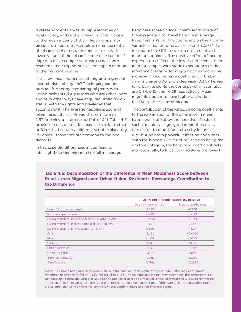
2.37, implying a migrant shortfall of 0.11. Table 4.5

provides a decomposition exercise similar to that

of Table 4.4 but with a different set of explanatory

variables - those that are common to the two

datasets.

In this case the differences in coefficients

add slightly to the migrant shortfall in average

happiness score (in total, coefficients’ share of

the explanation for the difference in average

happiness is -21%). The coefficient on the income

variable is higher for urban residents (0.173) than

for migrants (0.111), so raising urban relative to

migrant happiness. The positive effect of income

expectations reflects the lower coefficients in the

migrant sample: with static expectations as the

reference category, for migrants an expected big

increase in income has a coefficient of 0.21, a

small increase 0.00, and a decrease -0.37, whereas

for urban residents the corresponding estimates

are 0.34, 0.10, and -0.29 respectively. Again,

migrants appear to have higher aspirations

relative to their current income.

The contribution of the various income coefficients

to the explanation of the difference in mean

happiness is offset by the negative effects of

such variables as age, gender and the constant

term. Note that position in the city income

distribution has a powerful effect on happiness.

With the highest quarter of households being the

omitted category, the happiness coefficient falls

monotonically, to lower than -0.80 in the lowest

Table 4.5: Decomposition of the Difference in Mean Happiness Score between Rural-Urban Migrants and Urban-Hukou Residents: Percentage Contribution to the Difference

Using the migrants’ happiness function

Due to characteristics Due to coefficients

Log of income per capita 28.15 472.62

Income expectations -39.92 59.32

Living standard in second highest quarter in city -33.68 26.28

Living standard in third highest quarter in city -11.71 77.84

Living standard in lowest quarter in city 175.93 -8.37

Age 32.85 -594.05

Male -4.08 -46.78

Health -28.01 51.89

Other variables 1.14 36.97

Constant term 0.00 -96.38

Sum (percentage) 120.67 -20.67

Sum (score) 0.1342 -0.0230

Notes: The mean happiness scores are 2.4845 in the case of urban residents and 2.3703 in the case of migrants, creating a migrant shortfall of 0.1143 (set equal to +100%) to be explained by the decomposition. This represents 100 per cent. The composite variables are age and age squared for age, married, single, divorced and widowed for marital status, and big increase, small increase and decrease for income expectations. ‘Other variables’ are education, marital status, ethnicity, CP membership, unemployment, working hours and net financial assets.


quarter. As this is true of both samples, it does

not affect relative happiness.

The migrant shortfall in happiness therefore has

to be explained in terms of differences in average

characteristics (the total share of characteristics in

accounting for the difference in average happiness

is 121%). Two variables stand out: the higher

mean income of urban residents improves their

relative happiness, and their superior position in

the city income distribution has the same effect.

A far higher proportion of migrants than of urban

residents fall in the lowest quarter of city house-

holds in terms of living standard (35% compared

with 11%). This fact alone can explain more than

the entire migrant deficit. If the income of the

relevant comparator group influences aspirations,

the inferior position of migrants in the city

income distribution can also explain why they

appear to have higher aspirations in relation to

their current income.

7. Are Migrants Self-Selected?

It is evident that differences in unobserved

characteristics are important for the differences

in happiness. For example, the constant term in

the decomposition presented in Table 4.4 explains

more than the entire difference in the average

happiness scores of migrants and rural-dwellers.

Migrants might be less happy on average simply

because inherently unhappy people tend to be

the ones who migrate. Support for this idea comes

from answers to the question as to whether urban

living had yielded greater happiness than rural

living. Despite the average happiness score being

lower for migrants than for rural people, 56% of

migrants thought that urban living made for

greater happiness and only 3% disagreed. This is

the picture that could emerge if migrants are

intrinsically unhappy people whose happiness

remains low despite improving after migration.

Migrants might be unhappy people because by

nature they are melancholy or they have high but

unfulfilled aspirations. However, the latter reason

fits ill with the stereotype of migrants as relatively

self-confident, optimistic, risk-loving individuals.

Consider the implications of assuming both that

migrants are naturally unhappy people and that

migration does indeed generally raise happiness.

Insofar as those migrants with a relatively unhappy

disposition become absolutely happier albeit still

relatively unhappy after migration, we might

expect as high a proportion of unhappy as of

happy migrants to report that their life is more

satisfactory in urban than in rural areas. In fact

the proportion falls, from 67% in the highest

happiness category to 34% in the lowest

Figure 4.3: Rural-Urban Migrant and Urban Dweller (with Urban Hukou) Coefficients of Variables Denoting Expectations of Income in the Next Five Years, Derived from Happiness Functions Estimated for Table 4.5

0.50

0.40

0.30

0.20

0.10

0.00

-0.10

-0.20

-0.30

-0.40

-0.50

Co

effi

cie

nts

R-U migrants Urbanl dwellers

Expect big increase in income

Expect small increase in income

Expect decrease in income

80

81

happiness category, suggesting that this sort

of self-selection can at best be only a partial

explanation for the lower average happiness

of migrants.

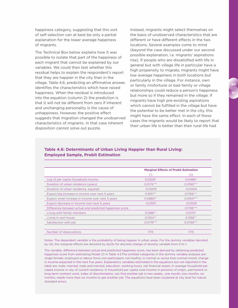
The Technical Box below explains how it was

possible to isolate that part of the happiness of

each migrant that cannot be explained by our

variables. We could then test whether this

residual helps to explain the respondent’s report

that they are happier in the city than in the

village. Table 4.6, predicting an affirmative answer,

identifies the characteristics which have raised

happiness. When the residual is introduced

into the equation (column 2) the prediction is

that it will not be different from zero if inherent

and unchanging personality is the cause of

unhappiness. However, the positive effect

suggests that migration changed the unobserved

characteristics of migrants. In that case inherent

disposition cannot solve out puzzle.

Instead, migrants might select themselves on

the basis of unobserved characteristics that are

different or have different effects in the two

locations. Several examples come to mind

(beyond the case discussed under our second

possible explanation, i.e. migrants’ aspirations

rise). If people who are dissatisfied with life in

general but with village life in particular have a

high propensity to migrate, migrants might have

low average happiness in both locations but

particularly in the village. For instance, own

or family misfortune or bad family or village

relationships could reduce a person’s happiness

but more so if they remained in the village. If

migrants have high pre-existing aspirations

which cannot be fulfilled in the village but have

the potential to be better met in the city, this

might have the same effect. In each of these

cases the migrants would be likely to report that

their urban life is better than their rural life had

Table 4.6: Determinants of Urban Living Happier than Rural Living: Employed Sample, Probit Estimation

Marginal Effects of Probit Estimation

(1) (2)

Log of per capita household income 0.0506* 0.0466*

Duration of urban residence (years) 0.0174*** 0.0190***

Duration of urban residence, squared -0.0003 -0.0004

Expect big increase in income over next 5 years 0.1657** 0.1766***

Expect small increase in income over next 5 years 0.0869** 0.0941***

Expect decrease in income over next 5 years -0.0557 -0.0559

Difference between actual and predicted happiness score 0.1736***

Living with family members 0.1286** 0.1070*

Living in own house 0.1304** 0.1286**

Satisfaction with job 0.0719*** 0.0768***

Number of observations 1715 1715

Notes: The dependent variable is the probability of being happier in urban areas. For the dummy variables denoted by (d), the marginal effects are denoted by dy/dx for discrete change of dummy variable from 0 to 1.

The variable, difference between actual and predicted happiness score, has been derived by obtaining predicted happiness score from estimating Model (1) in Table 4.3.The omitted categories in the dummy variable analyses are: single female; employed or labour force non-participant; not healthy; in normal or worse than normal mood; change in income expected in the next five years. Explanatory variables estimated in the equations but not reported in the table are: male, married, male and married, education, working hours, net financial assets, ln average household per capita income in city of current residence, ln household per capita rural income in province of origin,, permanent or long-term contract work, index of discrimination, can find another job in two weeks, .one month, two months, six months, needs more than six months to get another job. The equations have been clustered at city level for robust standard errors.


been, despite their low average urban happiness.

A test of this type of explanation would require

a survey which could reveal the happiness

score, and the reasons given for unhappiness,

before migrating

8. Other China Studies

One other study deals specifically with migrants.25

It analysed the China Household Income Project

(CHIP) survey [also known as the Rural-Urban

Migration in China (RUMIC) survey] relating

mainly to 2007. The research interest is in the

effects of various measures of relative income on

happiness. The data differed from that used in

the analysis above in that it contained all rural

hukou people present in the urban areas, i.e.

both temporary and settled migrants, and the

dependent variable was an aggregation of

twelve measures of mental health.

It was found that subjective well-being is

negatively affected by the incomes of other

migrants and of workers in the home region.

However, a positive coefficient was obtained

on average income in the local urban area.

This was interpreted as a ‘signal’ effect, i.e. the

higher incomes of urban people served as a

signal of future income prospects. A similar

positive coefficient had been obtained and

similarly explained for Russia.26 It contrasts

sharply with our finding of a negative coefficient.

The contrast was explained as arising because

our sample contained only settled migrants,

who were more likely to have transferred their

reference group from the village to the city. In

support of this explanation, it was noted that

the positive coefficient declined with years

since migration. Containing very different

definitions both of a migrant and of subjective

well-being, the two analyses are not necessarily

contradictory.

Technical Box

The argument can be tested rigorously as

follows. Estimating the predicted happiness

score for each respondent (from column 2

of Table 4.2), the residual (actual minus

predicted) score is the part of happiness

that cannot be explained by our equation.

The residual is made up of measurement

error and two sorts of unobserved

characteristics of the respondent: those

which were present before migration and

those which came after migration. A

disposition to be happy or unhappy is of

the former sort. Assume that migration

had a similar effect on the happiness of

all respondents whose unobserved

characteristics did not change pre- and

post-migration. In that case, we can test

whether the residual helps to explain

whether the respondent reported that

their happiness was higher in the city than

in the village.

Table 4.6 shows the results of a Probit

regression predicting an affirmative answer.

Its two columns, presenting the marginal

effects of each explanatory variable, both

refer to the employed sample. The object is

to identify the characteristics which have

raised happiness. Comparing Tables 4.2 and

4.3 (using OLS) with Table 4.6 (using Probit),

we see that some of the same variables that

determine happiness also correspondingly

determine an increase in happiness. When

the residual is introduced into the equation

corresponding to column 2 of Table 4.6, the

expectation is that it will not be significantly

different from zero if inherent and unchanging

personality is the cause of unhappiness.

However, the coefficient is positive and

significantly so at the 1% level (column 2),

and the marginal implies that a residual of

+1.0 raises the probability of an affirmative

answer by 17 percentage points. This

positive effect suggests that migration

changed the unobserved characteristics of

migrants, in which case inherent disposition

cannot solve the puzzle.

82

83

Another study examined the changes in the

average happiness of urban, rural, and rural-

urban migrant households between the CHIP

2002 and CHIP 2013 national household surveys.27

The ratio of migrants’ to rural households’

income per capita was higher in 2013 than it had

been in 2002: again, the economist’s expectation

is that rural people would have an incentive to

migrate to raise their utility. However, the average

happiness of rural-dwellers remained higher than

that of migrants, although the gap had narrowed.

The rise in migrant happiness was probably due

to the rapid growth of their income, associated

with the growing scarcity of migrant labour, and

gradual (but minor) improvements in their urban

treatment and conditions in recent years. We

surmise that the fall in average rural happiness,

despite a rise in average rural income, was

because the loss of household members to the

cities often left unbalanced families and villages

behind, or because rural households’ aspirations

rose rapidly as their information about urban

life improved.

9. Studies in Other Developing Countries

To what extent can the China story be

generalised? In one respect – the harsh

institutional and policy treatment of rural hukou

migrants in the cities – China is likely to be

exceptional. However, in many countries rural-

urban migrants are at a disadvantage: their

social networks are often weak, their education

is liable to be of poor quality for urban life and

work, and their village customs and weak

assimilation might cause social discrimination.

However, the available evidence cannot provide

a clear answer to this question. It appears that

research on the relationship between rural-urban

migration and happiness in developing countries

remains very limited.

Whereas our China case study found that

migration may well have had the consequence

of reducing subjective well-being, a study of

Thailand found that a somewhat higher propor-

tion of the permanent migrants in that sample

experienced an increase in life satisfaction after

migration than experienced a decrease.28

The interpretation of our main finding in terms

of changing reference groups is echoed in a

pioneering study for developing countries of

aspirations relative to achievement which

examined ‘frustrated achievers’ in Peru. More

than half of those who had objectively achieved

the largest income growth subjectively reported

that their economic condition had deteriorated

over the previous decade. Part of the explanation

was to be found in their perception of increased

relative deprivation.29

In South Africa a very extensive system of

temporary circular migration prevailed in the

past. However, since the advent of democracy

the country has increasingly experienced the

permanent urban settlement of rural-dwellers.

The same question has been posed for South

Africa as was posed above for China.30 That

study reached similar results and suggested

some of the same interpretations but used a

different methodology. A longitudinal panel

survey identified the happiness of rural people

and their happiness four years later after

rural-urban migration (excluding temporary

migration). The real income of the migrants rose

substantially, largely because of their migration.

Yet sophisticated estimation yielded a fall in

subjective well-being (measured on a scale of 0

to 10) of 8.3%. A favoured interpretation was that

this reduction was the result of false expectations

and changing reference groups after the migrants

settled in the urban areas.

10. Summary and Conclusion

This chapter illustrates how it should be possible

to go beyond a description of happiness and

its correlates. Using microeconomic (individual

and household) data based on a well-designed

survey and questionnaire, microeconomic

analysis can be used to explore and to answer

interesting and important questions about what

makes people happy or unhappy. The settled

rural-urban migrants that we study are the

vanguard of a great wave of settlement as the

urban economy becomes increasingly dependent

on migrants from rural China.

We have posed the question: why do rural-urban

migrant households which have settled in urban

China report lower happiness than rural house-

holds? Migrants had lower average happiness

despite their higher average income: the income

difference merely adds to the puzzle. It is a


question that cannot easily be answered in terms

of economists’ conventional models of rural-

urban migration based on ‘utility maximisation’.

Four possibilities were examined. We found

no evidence for the idea that happiness was

reduced by the need for the migrants to provide

support for family members in the village.

Each of the other three possibilities involves

false expectations, of three different types:

prospective migrants may have false expectations

about their urban conditions, or about their

urban aspirations, or about themselves. What

they have in common is that rural-urban migrants

are likely to lack the necessary information to

enable them to judge the quality of their new

lives in a different world. For each of the three

types of belief there are reasons why they are

too optimistic about life in the city.

Consider first the idea that migrants are too

optimistic about the conditions of city life. The

fact that happiness appears to rise over several

years suggests that migrants are able to over-

come the early hardships of arriving, finding

work, and settling in the city. However, some

hardships remain, relating to accommodation,

family, and work. Provided that accurate

information had been available to prospective

migrants, they should have taken account of

adverse conditions reducing their happiness

when deciding to migrate: expectations would

not have been false. Why might migrants

overestimate the conditions of their urban life

and work? It is possible that, whereas expected

income is quantifiable and understandable, other

aspects of urban life have to be experienced

to be understood. Moreover, expectations of

conditions might be based on images of the

lives of urban residents rather than those of

rural-urban migrants, or the reports provided

by migrant networks might be too rosy. The

migrants, when they made their decisions to

move, may have been realistic about their urban

income prospects, whereas their expectations

of living and working conditions could have been

biased upwards. However, there is a caveat:

the better the information flows to the villages,

the weaker is the case for this possibility.

The second possibility is that migrants had

falsely believed, at the time of migration, that

their aspirations would not alter in the city.

Consider the reasons why migrants’ aspirations

may have risen and now exceed their actual

achievements. When we conducted a decompo-

sition analysis to discover why migrants have a

lower mean happiness score than both rural

dwellers and urban dwellers possessing urban

hukous, in each case a major contribution came

from the higher aspirations of migrants in relation

to current income. This is consistent with the fact

that over two-thirds of migrants who were

unhappy or not at all happy gave low income as

the predominant reason for their unhappiness.

The relatively high aspirations might be explained

by the lowly position of most migrants in the city

income distribution: having relatively low income

was shown to reduce their happiness. The

evidence suggests that migrants draw their

reference groups from their new surroundings,

and for that reason have feelings of relative

deprivation. It is plausible that migrants, when

they took their decisions to move, could predict

that their incomes would rise but not how their

aspirations would rise as they became part of

the very different urban society.

Consider the possibility that people with

unobserved and invariant characteristics that

reduce happiness have a higher propensity to

migrate, in the false expectation that migration

will provide a cure, and that their continuing

unhappiness pulls down the mean happiness

score. However, our test using the residual,

unexplained component of individual happiness

scores provided no support for this argument.

Inherent disposition is unlikely to provide a good

explanation for the low average happiness score

of migrants.

There are other possible explanations which

cannot be adequately tested by means of our

data set. The one mentioned above is that

migration is subject to ‘selection bias’ on the

basis of unobserved characteristics which are

different or have different effects in the two

locations. Another is that rural-urban migrants,

once they settle in the city, are induced by

urban cultural norms to use a different scale

for measuring happiness, and thus to report

happiness scores lower than those of rural

residents. We would expect the reported

happiness of migrants to be higher before

they have time to adjust their happiness scale.

However, the average happiness score of

migrants who have been in the city for less than

three years is 0.08 points lower than the average

for all migrants, and the regression results in

84

85

Tables 4.3 and 4.4 suggest that the standardised

happiness score rises for more than a decade

after arrival. Although it is not possible to refute

the rescaling explanation, this evidence fails to

confirm it. Yet another possibility is that migrants

are willing to sacrifice current happiness for

future happiness - plausible in a country with

an overall household saving rate of no less than

24%. Migrants might be willing to put up with

unhappiness because they feel that life will

eventually get better for them or their children.

Analysis of the 2002 CHIP survey found that a

reason for the high happiness of rural-dwellers is

that they place a high value on village personal

and community relationships (Knight et al.,

2009). A further possible contribution to the

lower happiness of rural-urban migrants is

that they come to realise that their social

environment is less friendly and less supportive

than it was in the village.

The absence of tests for these alternative

explanations means that our conclusions have

to be qualified. Further research based on better

data sets is required to explain the puzzle in

China and, if it is found to be a general

phenomenon, in other poor urbanising societies.

Whatever the explanation, the obvious question

arises: why do unhappy migrants not return to

their rural origins? One reason is that the majority

do perceive urban living to have yielded them

more happiness than rural living. This result was

found to be sensitive to expected income, and

the majority of migrants did indeed expect that

their incomes would rise over the next five years.

Migrants were also more likely to favour urban

living the longer they stayed in the city – possibly

because they increasingly valued aspects of

urban living that were not to be found in rural

areas. Social psychology might again be relevant:

migrants do not take into account how their

aspirations will adjust if they return to village life.

Alternatively, migrants might correctly expect

that their new aspirations will not adjust back. So

there might be symmetry in the way they view

leaving their rural residence and not leaving their

urban one. Another possible reason why unhappy

migrants do not return to their origins – unfortu-

nately not pursued in the survey - is that the cost

might be prohibitive. This is plausible if their

households have forgone the tenurial rights to

village farm land and housing land that they

previously held.

The main policy instrument available to a

government that is concerned to improve the

subjective well-being of rural-urban migrants is

to reform the range of institutions and policies

which place the migrants at a disadvantage in

the cities. In some respects, however, migrants

might have to take the initiative. There is scat-

tered evidence that some rural-urban migrants

have created a more supportive and helpful city

environment for themselves - where migrants

from the same village, county or area choose to

concentrate in particular parts of a city.

The study has broader implications. Should

social evaluation by policy-makers reflect

measured happiness? The contrary argument

has been examined and found wanting.31 The

distinction made above between expected utility

(which economic agents are assumed to

maximise) and experienced utility (which

happiness scores are assumed to measure) is

relevant. Insofar as there is a systematic

difference between the two, this can arise

because of an unpredicted change in aspirations,

for instance, owing to a change in reference

group. In our judgement, changes in aspirations

should be taken into account in assessing

people’s perceptions of their own welfare. To

regard some objectively based ‘true’ utility

as existing separately from subjectively

perceived utility is effectively to make a

normative judgement about what is socially

valuable.

In many developing countries rapid rural-urban

migration gives rise to various social ills – such as

urban poverty, slums, pressure on infrastructure,

unemployment and crime – which adversely

affect the welfare of all urban residents. In

contrast, by attempting to restrict migration the

Chinese government has curbed these outcomes.

For instance, in the 2002 national household

survey few urban hukou residents reported that

the presence of migrants constituted the greatest

social problem - well behind corruption, lack of

social security and environmental pollution. The

fact that rural-urban migrants were the least

happy group suggests that they themselves might

foment unrest. However, because social instability

probably requires not only unhappiness but also

a perception that it is man-made and capable of

being remedied, no such conclusion can be

safely drawn.


The ongoing phenomenon of internal rural-urban

migration in developing countries involves many

millions of the world’s poor. Not only their

objective well-being but also their subjective

well-being deserves more extensive and more

intensive research. There is much to be done,

both to advance understanding and to assist

policymaking.

86

87

Endnotes

1 China’s rate of natural increase of the urban population was low on account of the one-child family policy, and much reclassification was the result of migration from rural areas.

2 Knight and Song (1999: chs. 8,9)

3 Zhao (1999).

4 Knight and Song (1999: ch.9; 2005, chs.5,6).

5 Knight and Yueh (2008).

6 Gao et al. (2017: 285). These labour force figures are of course lower than the urban population figures of Table 4.1.

7 Knight et al. (2011: 597)

8 Knight et al. (2010: table 1).

9 Organised by the Institute of Economics, Chinese Academy of Social Sciences, and designed by Chinese and foreign scholars including one of the authors.

10 In several papers but especially Easterlin (2003).

11 The explanation draws on the psychological literature to make the distinction between ‘decision utility’ and ‘experienced utility’: the utility expected at the time of making a choice and the utility subsequently experienced from that choice.

12 Rabin (1998:12).

13 At least as far back as Runciman (1966).

14 Knight et al. (2009); Knight and Gunatilaka (2010).

15 Clark et al. (2008).

16 Graham and Pettinato (2002), Senik (2004).

17 Kingdon and Knight (2007).

18 Fafchamps and Shilpi (2008).

19 Unless a variable is both important to our story and likely to be endogenous (as in the case of income, discussed below), we interpret the coefficients as indicating causal effects on happiness.

20 First, happiness was made a binary variable and estimated by means of a probit model; secondly, happiness was converted into a multinomial variable and estimated with an ordered probit model. The pattern of results was very similar to that of Table 4.3.

21 The same specification as in Table 4.3 (column 2) with the potentially endogenous variable that is most relevant to our tests, log of income per capita, now instrumented. The exclusion restrictions are mother’s years of education, spouse’s years of education, and the income that the migrant earned in the village before migrating, It is plausible that these variables do not directly influence current happiness (not even own happiness has a positive effect in Tables 4.3 and 4.4). The instrument passed the conventional tests.

22 The coefficient on income was raised but the effect was modest. One possible explanation for the rise is that hidden relationships have the opposite sign, e.g. higher aspirations raise income but lower happiness, or happiness discourages effort.

23 Fortunately, few observations are lost.

24 With zero remittances set equal to one yuan.

25 Akay et al. (2012).

26 Senik (2004).

27 Luo (2017).

28 De Jong et al. (2002).

29 Graham (2005).

30 Mulcahy and Kollamparambil (2016).

31 Clark et al. (2008).

References

Akay, Alpasian, Oliver Bargain, and Klaus F. Zimmermann (2012). Relative concerns of rural-to-urban migrants in China, Journal of Economic Behavior and Organization, 81: 421-41.

Clark, Andrew, Paul Frijters and Michael Shields (2008). Relative income, happiness and utility: an explanation of the Easterlin Paradox and other puzzles, Journal of Economic Literature, 46, 1: 95-144.

De Jong, Gordon, Aphichat Chamrarrirthirong, and Quynth- Giang Tran (2002). For better, for worse: life satisfaction consequences of migration, International Migration Review, 36, 3: 838-63.

Easterlin, Richard A. (2001). Income and happiness: towards a unified theory, Economic Journal, 111, July: 465-84.

Fafchamps, M. and F. Shilpi (2008). Subjective welfare, isolation and relative consumption, Journal of Development Economics, 86, 1: 43-60.

Graham, Carol (2005). Insights on development from the economics of happiness, World Bank Research Observer, 20, 2, Fall: 201-32.

Graham, Carol and Stefano Pettinato (2002). Frustrated achievers: winners, losers and subjective well-being in new market economies, Journal of Development Studies, 38, 4: 100-40.

Knight, John, Deng Quheng and Li Shi (2011). The puzzle of migrant labour shortage and rural labour surplus in China, China Economic Review, 22: 585-600.

Knight, John and Ramani Gunatilaka (2009). Great expectations? The subjective well-being of rural-urban migrants in China, World Development, 38, 1: 113-24.

Knight, John and Ramani Gunatilaka (2010). The rural-urban divide in China: income but not happiness?, Journal of Development Studies, 46, 3, March: 506-34.

Knight, John and Ramani Gunatilaka (2012). Aspirations, adaptation and subjective well-being of rural-urban migrants in China, in David A. Clark (ed), Adaptation, Poverty and Development. The Dynamics of Subjective Well-being, Basingstoke: Palgrave Macmillan, 91-110.

Knight, John, Li Shi and Deng Quheng (2010). Education and the poverty trap in rural China, Oxford Development Studies, 38, 1, March: 1-24.

Knight, John and Lina Song (1999). The Rural-Urban Divide. Economic Disparities and Interactions in China, Oxford: Oxford University Press.

Knight, John and Lina Song (2005). Towards a Labour Market in China, Oxford: Oxford University Press.

Knight, John, Lina Song and Ramani Gunatilaka (2009). The determinants of subjective well-being in rural China, China Economic Review, 20: 635-49.

Knight, John and Linda Yueh (2008). Segmentation or competition in China’s urban labour market?, Cambridge Journal of Economics, 33, 1: 79-94.

Luo Chuliang (2017). Income growth and happiness growth in China, Economic and Political Studies, 5, 3, September: 266-84.

Mulcahy, Kirsten and Umakrishnan Kollamparabil (2016). The impact of rural-urban migration on subjective well-being in South Africa, Journal of Development Studies, 52, 9: 1357-71.

Rabin, M. (1998). Psychology and economics, Journal of Economic Literature, 36, March: 11-46.

Runciman, W. G. (1966). Relative Deprivation and Social Justice, Berkeley: University of California Press.

Senik, Claudia (2004). When information dominates comparison: learning from Russian subjective panel data, Journal of Public Economics, 88: 99-123.

Zhao, Yaohui (1999). Labor migration and earnings differences: the case of rural China, Economic Development and Cultural Change, 47: 766-82.


rural-urban migration and happiness in china · migration and on subjective well-being in...

Documents