rs ' oftumentation pagefomave ad- a283 368

rs ' OftUMENTATION PAGEFomAve

AD- A283 368 i W-a~ftWg"M~~~~~l" MW~0 kftfWWIAb M O WWbs fdAat". 1215 JdISSCI OR*4 HlVMwe. 51*. 1204. A*.gQa VA O2.43= wPW M(o04.o8), WnlhWl. DC 205.Report Date. 3. Report Type and Date. Covered.1994 .Final -Journal Article

a. rue a bubUlle. 5. Funding Numbers.Magnetospheric and Ionospheric Signals in Magnetic Observatory Monthly Means: Program EemewnNo. 0601153NElectrical Conductivity of the Deep Mantle Pro/ot. 03204

6. Author(s). Task NA. 360

McLeod, Malcolm G. Accessbon NA. DN258032

Work unit NA. 574506503

7. Performing Organization Name(s) and Address(es). 8. Performing OrganizationNaval Research Laboratory Report Number.Mapping, Charting and Geodesy Branch Journal of GeophysicalStennis Space Center, MS 39529-5004 Research, Vol. 99. No. B7, pp.

13,577-13,590, July 10, 1994

9. SponsoringlMonitoring Agency Name(s) and Address(e*). 10. Sponsoring/Monitoring Agency

Naval Research Laboratory Report Number.

Center for Environmental Acoustics NRUIJA7442-93-0012Stennis Space Center, MS 39529-5004 '

11. Supplementary Notes. L OTu% 7 1994

12a. Distrlbution/Avallablity Statement . 12b. Distribution Code.Approved for public release; distribution is unlimited.

13. Abstract (Maximum 200 words).

First differences of magnetic observatory monthly meansfor 1963-1982 were analyzed using techniques of spherical harmonic _analysis and power spectral analysis. The external source signal is shown to be primarily zonal in geomagnetic coordinates.Prominent peaks are present in the power spectrum at frequencies of 1.0 cycle/yr and 2.0 cycles/yr. The annual signal is largeston the degree 2 external zonal spherical harmonic, while the semiannual signal is largest on the degree 1 and degree 3 externalzonal spherical harmonics. The presence of the semiannual signal on odd-degree spherical harmonics and of the annual signal 0on even-degree spherical harmonics was predicted from symmetry considerations and of the annual cycle of solar inclination.---These signals are all modulated by the sunspot frequency and its harmonics. The degree 1 term is believed to be due mainlyto magnetopause and ring currents while the degree 2 and degree 3 terms are believed to be due mainly to ionospheric currents.The degree 1 external zonal harmonic has a continuous spectrum in addition to the semiannual spectral peak. A correspondingdegree 1 internal term is due to electromagnetic induction. The degree 1 continuous spectrum is useful for study of the electricalconductivity of the deep mantle. A global geomagnetic response function consistent with a mantle conductivity of about 10 S/0o esm at the core-mantle boundary has been derived. Avail and/o

I~iot / Special

14. Subject Terms. 15. Number of Pages.Geomagnetism; Magnetic Observatory Monthly Means; Harmonic Analysis; Spectral Analysis 14

16. Price Code.

17. Security Classification 18. Security Classification 19. Security Classification 20. Umltation of AbstracLof Report, of This Page. of Abstract.

Unclassified Unclassified Unclassified SAR

NSN 7540-01-280-5500 Standwd Form 23 (Rev. 2-89)-Wb ANSI0 SOL 0-2

JOURNAL OF GEOPHYSICAL RESEARCH, VOL. 99, NO. B7, PAGES 13,577-13,590, JULY 10, 1994

Magnetospheric and ionospheric signals in magnetic observatorymonthly means: Electrical conductivity of the deep mantle

Malcolm G. McLeodNaval Research L.aboratory, Stennis Space Center, MfississippiIS dAbstrat. First differences of magnetic observatory monthly means for 1963-1982were analyzed using techniques of spherical harmonic analysis and power spectral (Danalysis. The external source signal is shown to be primarily zonal in geomagneticcoordinates. Prominent peaks are present in the power spectrum at frequencies of 1.0cycle/yr and 2.0 cycles/yr. The annual signal is largest on the degree 2 external zonalspherical harmonic, while the semiannual signal is largest on the degree 1 and degree 3external zonal spherical harmonics. The presence of the semiannual signal on odd- smut1degree spherical harmonics and of the annual signal on even-degree spherical = Wharmonics was predicted from symmetry considerations and the annual cycle of solar ainclination. These signals are all modulated by the sunspot frequency and itsharmonics. The degree 1 term is believed to be due mainly to magnetopause and ringcurrents while the degree 2 and degree 3 terms are believed to be due mainly to 00ionospheric currents. The degree I external zonal harmonic has a continuous spectrumin addition to the semiannual spectral peak. A corresponding degree I internal term isdue to electromagnetic induction. The degree 1 continuous spectrum is useful for studyof the electrical conductivity of the deep mantle. A global geomagnetic responsefunction consistent with a mantle conductivity of about 10 S/m at the core-mantleboundary has been derived.

Introduction defined as the transfer function between the induced internalspherical harmonic and inducing external spherical har-

The geomagnetic field at Earth's surface consists of two monic; the existence of a conductivity which is a functionparts: a part due to sources within Earth's surface and a part only of radial distance and which relates the current densitydue to sources outside Earth's surface. These two parts of linearly to the electric field is assumed.the geomagnetic field can in principle be separated from each Much of the methodology associated with estimation ofother by the method of spherical harmonic analysis devel- geomagnetic response functions is due to Banks [1969].oped in 1838 for the magnetic potential function by C. F. Banks showed that for periods greater than a day and lessGauss. This method is based on the assumption that no than a year the geomagnetic spectrum is primarily due to asignificant electric currents cross Earth's surface. degree I external field aligned with Earth's magnetic dipole

External sources of the geomagnetic field include electric axis. He showed that in addition to a continuous spectrumcurrent systems within Earth's magnetosphere and iono- there are discrete annual and semiannual lines in the spec-sphere and on the magnetospheric boundary, which is called trum and that the annual line is primarily a degree 2 externalthe magnetopause [Potemra, 1991; Russell and Luhmann, spherical harmonic aligned with Earth's magnetic dipole1991]. All of the external current systems vary with time axis. This confirmed results of an extensive analysis bybecause of varying solar activity. Study of that portion of the Currie [1966]. Currie concluded that ionospheric dynamogeomagnetic field due to external sources can reasonably be action is probably responsible for the annual variation, whileexpected to yield information on such geophysical parame- a ring current located about 3.5 Earth radii from Earth'sters as ionospheric ionization and its time variations. Thisinfomaton an i tun b execte toconribue t uner-center is the most likely source of the semiannual line. Theinformation can in turn be expected to contribute to under- semiannual line had been previously resolved by Eckhardt etstanding of the mechanisms by which ionization is created in al. [1963]. Banks thought, as did Currie, that the ring currentthe ionosphere. was the source of the external degree I spectrum. However,

Time variations of the external electric current systems the next section will show that there are reasons to believeproduce time-varying magnetic fields that induce electric that at least part of the external degree I spectrum is due tocurrents within Earth by electromagnetic induction. electric currents on the magnetopause.Schuster [1889] demonstrated the possibility of obtaining Achache et al. [1981] discussed the numerical computa-knowledge of the radial distribution of Earth's electrical tion of the geomagnetic response function from Earth'sconductivity from observations of time variations of the con of ile Theyic responsegeomagnetic field due to external sources. The geomagnetic conductivity profile. They computed the degree I responseresponse function for a given degree spherical harmonic is function for three conductivity profiles previously proposed

by McDonald [1957], Banks [1969], and Ducruix et al.This paper is not subject to U.S. copyright. Published in 1994 by the [1960]. They compared computed values of the responseS American Geophysical Union. function with values determined from measurements by

Paper number 94JB00728. other investigators for periods ranging from 20 days to 9

13,577

13,578 MCLEOD: MAGNETIC OBSERVATORY MONTHLY MEANS

years. They concluded that the profile proposed by Ducruix magnetic observatory data. These current systems haveet al. [1980] best fit the experimental data, but they stressed been reviewed by Potemra [1991], Russell and Luhmannthe need for more accurate determination of Earth's re- [1991], McLeod [1991], Matsushita [1967], and Campbell etsponse at low frequencies, particularly periods of a few al. [1989). There are four major external current systems asyears. McLeod [1992) determined the response function for described below. All of these current systems are modulateda 2-year period using magnetic observatory annual means for by solar activity.1962-1983 as a data source. He concluded that the profile A solar wind of ionized particles emanates continuallyproposed by Banks [19691 fit this new result better than the from the Sun. This wind confines the geomagnetic field to aother two profiles considered by Achache et al. [1981). The cavity that extends about 12 Earth radii from the center ofBanks profile is for a conductivity of approximately 10 S/m Earth in the solar direction. The cavity extends over 1000at the core-mantle boundary. Earth radii from Earth's center in the antisolar direction,

Constable [ 1993] proposed a global geomagnetic response beyond the orbit of the Moon, and is about 30 Earth radii infunction, sensitive to average radial electrical conductivity diameter at Earth in the direction perpendicular to the solarof Earth's mantle between 200 and 2000 km, obtained by direction. Dimensions of the cavity are mainly determinedaveraging response functions published by Roberts [1984] by pressure balance between solar wind pressure and pres-and Schultz and Larsen [1987]. The averages used in Con- sure attributable to the geomagnetic field.stable's study were estimates for periods ranging from 3.25 The cavity boundary is called the magnetopause. Electricdays to 3.4 months. His response function is consistent with currents flow on the magnetopause because the geomagnetica conductivity jump at a depth of 660 km from a value of field deflects ionized solar wind particles; these currents2 S/m below 660 km to a much smaller value above this produce a jump in magnetic field magnitude at the magneto-boundary. The boundary at 660 km corresponds to a seismic pause. Field magnitude is nearly zero external to the cavitydiscontinuity and a presumed phase transition for mantle while field magnitude internal to the cavity is increased frommaterial. Constable [1993] gives several references for re- what it would be if magnetopause currents were not present.cent work on mineral physics and geomagnetic induction in The jump in magnetic field magnitude at the magnetopausethe upper mantle. has been observed many times by spacecraft. Magnitude of

Another approach to the determination of mantle conduc- the jump is typically about 50 nT but may be much greatertivity involves measurement of the spectrum of signals that when the magnetopause is close to Earth. Magnetopauseoriginate in Earth's core. If the spectrum of the signals at the location varies with solar wind pressure, so that a spacecraftbase of the mantle is known (or assumed), then the radial moving away from Earth to interplanetary space may crosselectrical conductivity profile can be estimated from mea- the magnetopause several times on a single trajectory as thesurements of the spectra of these signals at Earth's surface. magnetopause moves back and forth past the spacecraft.The basic problem with this approach is that the spectrum of The magnetopause has been observed as close to Earth asthe input at the base of the mantle is not known. A variation 6.6 Earth radii [Russell, 1976]. Average solar wind pressureof this approach that uses assumed properties of the geo- varies with sunspot activity; consequently, the portion of themagnetic jerk of 1969 has been discussed by Backus [19831. average magnetic field at Earth's surface produced by mag-

In this paper, electrical current systems external to netopause currents varies with the solar cycle, which has anEarth's surface are briefly reviewed. Effects that these approximate II-year period.current systems should be expected to have on field models A ring current is located at about 3.5 Earth radii from theproduced from magnetic observatory monthly means are center of Earth. The ring current encircles Earth near thepredicted (or hypothesized) based on symmetry arguments. plane of the geomagnetic equator. The current is due toFirst differences of magnetic observatory monthly means for ionized particles trapped in the geomagnetic field. Average1963-1982 are analyzed using techniques of spherical har- ring current varies with solar activity and with the sunspotmonic analysis and power spectral analysis. Results of this cycle.analysis are compared with the predictions and are shown to The magnetic field produced by the ring current at Earth'sbe in good agreement. Except for Earth's auroral regions, surface is approximately in the opposite direction to the fieldthe external source signal is shown to be primarily zonal in produced by magnetopause currents. Both of these currentgeomagnetic coordinates. The continuous spectrum is well systems are sufficiently far from Earth's surface that the fieldrepresented by zonal degree I spherical harmonics. The they produce can be well represented by degree I zonalcontinuous spectrum, with annual and semiannual spectral spherical harmonics in geomagnetic coordinates.lines excluded, is used in this paper to estimate a global Electric currents flow in the ionosphere at low latitudesgeomagnetic response function for periods ranging from 2 and midlatitudes due mainly to tidal effects and to iono-months to 2 years and sensitive to average radial electrical spheric heating by the Sun. Both mechanisms cause ionizedconductivity of the deep mantle down to the core-mantle particles to move in Earth's magnetic field; the field causesboundary. The estimated response function found here the charged particles to be deflected from what wouldagrees well with the response for the conductivity profile otherwise be their trajectories, and the deflection of theproposed by Banks [1969], as described by Achache et al. charged particles gives rise to electric currents. Ionospheric(19811, for which conductivity at the core-mantle boundary current systems have been reviewed by Matsushita [1967]is about 10 S/m. and Campbell et al. [1989]. The ionospheric current systems

are approximately symmetric about the Sun-Earth line andabout the geomagnetic equator at the times of the spring and

External Current Systems fall equinoxes. These current systems consist largely ofOur knowledge of external current systems is based current loops centered near the noon meridian at about ±-30

largely on observations from artificial Earth satellites and on geomagnetic latitude at the times of the equinoxes and are

MCLEOD: MAGNETIC OBSERVATORY MONTHLY MEANS 13,579

farther north or south at the times of the summer or winter tems move north and south on a seasonal basis, zonalsolstices, respectively. As Earth rotates beneath these cur- spherical harmonics of even degree should be expected atrent systems, the magnetic field components at a fixed the times of the solstices; thus these even-degree sphericallocation on Earth's surface exhibit a time variation with a harmonics should vary with an annual period and oddI-day period. This time variation is called daily variation, harmonics of the annual period. The odd-degree sphericalAmplitude and waveforms of daily variation are different for harmonics should vary with a semiannual period and itsdifferent geomagnetic latitudes and seasons of the year and harmonics. Averaged over an entire year, the even-degreefor different magnetic field components; a typical amplitude spherical harmonics should be zero, but the odd-degreeis t30 nT. spherical harmonics should not in general average to zero.

Another external current system consists of currents that Harmonics of the sunspot cycle and a constant or DCflow along magnetic field lines in Earth's magnetotail. The component should be expected for the odd-degree sphericalcurrents flow toward Earth on one side of the magnetotail harmonics. In general, a continuous spectrum due to randomand away from Earth on the other side of the magnetotail. variations in solar activity should be expected as well. TheThese two current flows are connected by currents flowing in preceding discussion is based on the fact that Earth's mainthe ionosphere near auroral latitudes. field is approximately a dipole; however, since other spher-

ical harmonics are small but significant at ionospheric alti-

Expectd Effects of External Current Systems tudes, the ionospheric source field should be expected to beon Magnetic Observatory Monthly Means less nearly zonal than are the fields due to magnetopauseBecMausetc t servatopause cuentsy Mand tcurrents or fields due to the ring current. The symmetry

Bemuse the magnetopause currents and the ring current approximations are also less nearly exact at Earth's surfaceare located far from Earth's center, they should be expected for the ionospheric source field than for the magnetopause

to produce a nearly uniform field, that is, a degree 1 field, for the onospheric s urcef t foe m n pover the entire surface of Earth. Because the ring current is source field or for the ring current field.caused by particles trapped in the geomagnetic field, whichis primarily a dipole field at the location of the ring current, Data Set Selectionand because the magnetopause currents cancel Earth's di- Data used in this study are magnetic observatory monthlypole field external to the magnetosphere, both of these means obtained from the National Geophysical Data Centercurrent systems should be expected to produce fields aligned (NGDC) operated by the National Oceanic and Atmosphericwith or opposed to Earth's dipole. A constant or DC Administration (NOAA) of the U.S. Department of Corn-component should be expected, and since solar activity merce. The data were on a compact disk (CD-ROM) labeledvaries with the sunspot cycle, harmonics of the sunspot NGDCOI. The data set chosen for the study consisted of thecycle should also be expected. The size of the magneto- monthly means of the vector field components from anysphere should be expected to vary seasonally as the strength magnetic observatory that had three-component vector dataof the dipole field at the subsolar point varies. The ring manytcalendar th. he chrenomont mean dancurrent also should be expected to vary seasonally as the for any calendar month. The chosen monthly mean is anangle between Earth's axis and the Sun-Earth line varies, average for all days of the month and all times of day. Mostsince this could affect insertion of ionized particles into the of the analyses in this paper are for the 20-year time intervalring current. There could also be an effect caused by from 1963 to 1982, although a few illustrations are for theseasonal variation of the solar latitude of Earth's orbital 60-year interval from 1923 to 1982. The observatories are notposition. Symmetry considerations suggest that the seasonal uniformly distributed about Earth; they are concentrated invariation should have a semiannual period and, in general, Europe and Japan with relatively few located south of theharmonics of that semiannual period. A continuous spec- geomagnetic equator, defined here as the equator for thetrum resulting from random variations in solar activity geocentric magnetic dipole. The locations of the observato-should be expected also. ries are similar to those shown by McLeod [1992].

Because the ionospheric current systems do not rotate The selected data were lightly edited to reduce obviouswith Earth but are approximately fixed in local time, daily errors. Time series for the first differences of the monthlyaverages of the field produced by these current systems means for each observatory were computed. The first differ-should not be expected to have an east-west component. ences for a given month at a given observatory were rejectedThis is a consequence of Ampere's law for a potential field. if any first difference was greater than 200 nT/month. TheThus the average ionospheric source field should be approx- lightly edited first difference time series were used for allimately zonal in geomagnetic coordinates, provided the further studies described here.average is for an integral number of days and for a suffi- The data selection procedure described here for magneticciently long time. At the times of the equinoxes, symmetry observatory monthly means is similar to that for annualconsiderations suggest that the field should have primarily means described by McLeod [19921. Most of the analyses inS odd-degree zonal spherical harmonics in geomagnetic coor- this study are for nearly the same time interval used in the

S dinates, since Earth's dipole field is the principal field previous study, 1961-1983. Figure 1 shows the number of

S influencing these current systems. observatories with available first differences of monthly

SBecause the centers for the low-latitude and midlatitude means for each month in the time interval 1920-1990. The

Sionospheric current systems at the times of the equinoxes number of available observatories for each month in the

w:ae at ±t30• geomagnetic latitude, a relatively large degree 3 1963-1982 portion of this study varied from 29 to 113, with a

S Ihrical harmonic should be expected, together with a typical value of 45; in contrast, the same set of 73 observa-

! der degree 1 spherical harmonic and other odd-degree tories was used for each individual year in the previous

Sharmonics. Since the centers for the current sys- study.e.-


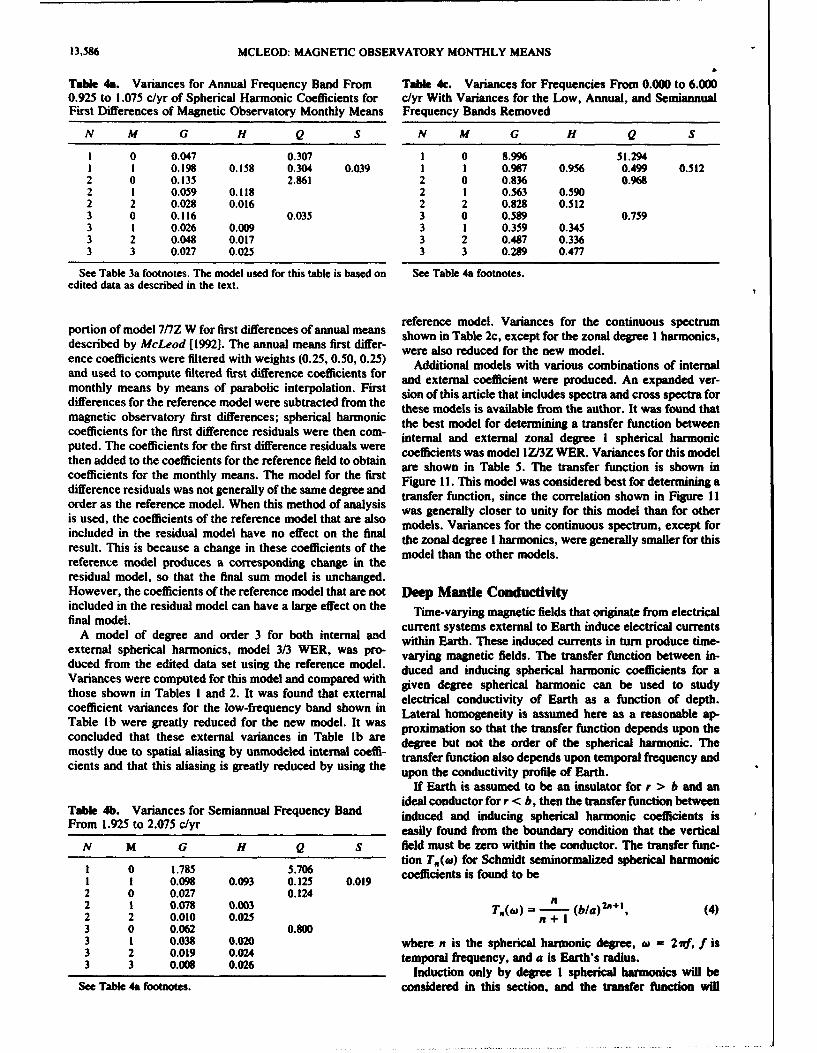
o ........ aliasing errors are larger and are shifted upward in temporalfrequency if the spherical harmonic analysis is done first,

100 -since not every observatory has data for the entire timeinterval selected for study.

Errors for each field component at each observatory were

estimated using the procedure described by McLeod [1992].Third differences of the measured monthly means werecomputed for each field component at each observatory.Third differences computed from a model field were sub-tracted from the measured third differences to obtain resid-ual third differences. The rms residuals were assumed to be

0 ..... .................................. good indicators of data quality, for reasons stated by80 40 5 McLeod [19921, and were used as weights for the weighted

least squares computation of spherical harmonic modelsFigure 1. Available magnetic observatory monthly means. used in this study.The number of observatories with available first differences The rms residuals are believed to be mostly noise andof monthly means is shown for each individual month in the auroral ionospheric source geomagnetic signals of sphericaltime interval 1920-1990. harmonic degrees that are too large to be modeled with

available observatory monthly means. Residuals were largefor auroral zone observatories, so data from these observa-

Data Analysis tories had little effect on the computed models.Spherical harmonic coefficients in geomagnetic coordi-

nates were computed for first differences of magnetic obser- Spectral Analysisvatory monthly means from the selected data set using aweighted least squares procedure. Fourier series for individ- Spherical harmonic coefficients for first differences ofual spherical harmonic coefficients were then determined monthly means for the 20-year time interval 1963-1982 wereand used to compute periodograms, power spectra, and spectrally analyzed. Power at each Fourier frequency forcross spectra. The analysis procedure is described in greater each coefficient was determined. The Fourier frequenciesdetail in the following sections. are multiples of the fundamental frequency, 0.05 cycle

per year (c/yr) from 0.00 c/yr to the Nyquist frequency,6.00 c/yr. This set of spectral estimates is sometimes called

Spherical Harmonic Analysis a periodogram; each estimate has 2 degrees of freedom.The method of spherical harmonic analysis used in this Power was computed for four different frequency bands:

study was the same as that used by McLeod [1992]. The (I) a low-frequency band from 0.000 to 0.125 c/yr for whichgeomagnetic field vector first differences and observatory power was found by summing the power for Fourier frequen-locations were transformed to a geomagnetic coordinate cies 0.00, 0.05, and 0.10 c/yr; (2) an annual frequency bandsystem. Geomagnetic coordinates are defined by a rotation from 0.925 to 1.075 c/yr for which power was found byof the geocentric coordinate system such that the axis of the summing the power for Fourier frequencies 0.95, 1.00, andgeomagnetic coordinate system coincides with the axis of 1.05 c/yr; (3) a semiannual frequency band from 1.925 toEarth's magnetic dipole. 2.075 c/yr for which power was found by summing the power

Spherical harmonic models of the first differences of the for Fourier frequencies 1.95, 2.00, and 2.05 c/yr; and (4) amagnetic observatory monthly means were constructed. It is band consisting of all other frequencies for which power wasvery important to the analysis that the first differences be found by subtracting the power for the previous threecomputed before the spherical harmonic analysis is per- frequency bands from the total power. The band limits givenformed, in contrast to first performing the spherical har- are approximations; the frequency window for a period-monic analysis on the monthly means and then computing ogram has sidelobes, as discussed by Marple [1987], but thefirst differences of the spherical harmonic coefficients. To frequency window is approximated here as a rectangularunderstand this, consider that the observatory monthly window with boundaries midway to the adjacent Fouriermeans contain nearly constant crustal source fields. When frequencies.first differences are calculated first, the effects of a constant Spectra and cross spectra were estimated for zonal degreebias in the monthly means is eliminated, so that the crustal I coefficients. Spectra were estimated from the period-source fields have almost no effect on the computed first ograms by averaging over frequency; the power for a givendifference spherical harmonic coefficients. If the spherical Fourier frequency was estimated as the average of theharmonic analysis had been performed first, the crustal periodogram power for that frequency and the five adjacentsource fields would produce spatial aliasing errors. Since not Fourier frequencies on each side of the given Fourier fre-every observatory is used for the full time interval selected quency. This method of spectral estimation, called thefor study, the aliasing errors would have discontinuities at Wiener-Daniell method, is discussed in many texts includingthe times when data from a particular observatory begins or Otnes and Enochson [1978], Marple 11987], and Gardnerends. These discontinuities would cause errors in the com- [1988]. The method was chosen because of its simplicity andputed first differences of the spherical harmonic coefficients. because of its relatively small frequency window sidelobes inThe same principle that applies to crustal source aliasing comparison to some other methods, such as the Bartletterrors applies to low-frequency spatial aliasing errors from method or the classic Blackman-Tukey method. Each spec-unmodeled core source spherical harmonics. That is, the tral estimate has 22 degrees of freedom; therefore the


Table Ia. Variances for All Frequencies From 0.000 to Table 2a. Variances for Annual Frequency Band From6.000 c/yr of Spherical Harmonic Coefficients for First 0.925 to 1.075 c/yr of Spherical Harmonic Coefficients forDifferences of Magnetic Observatory Monthly Means First Differences of Magnetic Observatory Monthly Means

N M G H Q S N M G H Q S

I 0 25.710 56.393 I 0 0.072 0.260I I 6.950 4.290 3.389 2.867 I I 0.072 0.077 0.050 0.1732 0 12.560 5.692 2 0 0.148 2.9312 I 9.433 5.141 3.508 4.519 2 1 0.024 0.100 0.404 0.5912 2 4.642 15.312 3.521 3.690 2 2 0.034 0.131 0.081 0.2513 0 2.972 3.643 3 0 0.037 0.0193 1 2.388 4.159 1.615 1.828 3 1 0.024 0.051 0.046 0.0623 2 3.071 2.614 2.398 1.402 3 2 0.029 0.045 0.070 0.1573 3 2.115 4.271 1.477 2.785 3 3 0.060 0.147 0.139 0.113

N and M are the degree and ordcr of the coefficients, G and H are N and M are the degree and order of the coefficients, G and H areinternal coefficients, and Q and S are external coefficients. Vari- internal coefficients, and Q and S are external coefficients. Vari-ances are mean square first difference fields associated with each ances are mean square first difference fields associated with eachcoefficient in units of (nT/mo) 2. coefficient in units of (nT/mo) 2.

standard deviation of a spectral estimate is 30% of the power The correlation R is defined byspectral density for the frequency corresponding to that R2 (CC*)I(SiS,), (2)spectral estimate. It is assumed that the underlying random (process is stationary, Gaussian, and ergodic and that the where the asterisk stands for complex conjugate. The stan-spectrum is flat over the range of frequencies used for the dard deviation aoT for the magnitude of T, (TT*) 1/2, isspectral estimate. Since these assumptions may not be valid,the stated standard deviation may be less than the true oar1/T= 0.30(1 - R2 )I 2 , (3)standard deviation. Low-frequency, annual, and semiannual where the cross-spectral estimate is assumed to have 22frequency bands were removed from the periodograms be- degrees of freedom.fore computing estimated spectra by setting the power equal Equation (3) yields an estimate of the error in the directionto zero for Fourier frequencies 0.00, 0.05, 1.00, 1.95, 2.00, of the complex vector T. Assuming that the estimated errorand 2.05 c/yr. In order to compute spectral estimates near in the direction perpendicular to T has the same value, thethe ends of the frequency range, it was assumed that the error in phase angle and in the real and imaginary parts of Tperiodograms are symmetric about the origin and Nyquist can be found.frequency.

Cross spectra between internal and external zonal degreeI spherical harmonic coefficients were computed in a similar Spatial and Temporal Spectramanner. The real part of the cross spectrum was assumed to Tables 1 and 2 show mean square values (variances) ofbe symmetric, and the imaginary part of the cross spectrum geomagnetic field first differences associated with eachwas assumed to be antisymmetric, about the origin and spherical harmonic coefficient in geomagnetic coordinatesNyquist frequency. for model 3/3 W. This model is of degree and order 3 for both

Let S, and S, be the power spectral density estimates for internal source and external source terms. Parameters G andthe external and internal zonal degree 1 spherical harmonic H are internal source spherical harmonic coefficients, whilecoefficients, and let C be the cross-spectral estimate for Q and S are external source spherical harmonic coefficients,these coefficients. If the coefficients can be related by a as described by McLeod [1992]. Parameters N and M aretransfer function T, an estimated value of T can be found degree and order, respectively, for the coefficients; thosefrom coefficients for which M = 0 are called zonal coefficients.

Variances are shown for four different frequency bands. TheT = C/Se. (1) first difference field variances were computed from the

Table lb. Variances for Low Frequencies From 0.000 to Table 2b. Variances for Semiannual Frequency Band

0.125 c/yr From 1.925 to 2.075 c/yr


I 0 14.336 0.456 I 0 1.368 4.657I I 3.196 0.134 1.307 0.094 1 1 0.101 0.207 0.054 0.1762 0 10.109 0.286 2 0 0.156 0.2352 1 7.626 1.859 1.362 0.611 2 I 0.092 0.120 0.058 0.0992 2 0.885 10.778 0.128 0.467 2 2 0.058 0.123 0.175 0.0613 0 1.110 0.278 3 0 0.176 1.4303 1 1.428 3.056 0.535 0.252 3 I 0.020 0.070 0.099 0.3313 2 0.927 1.053 0.092 0.129 3 2 0.013 0.051 0.193 0.0183 3 0.997 1.779 0.419 0.141 3 3 0.038 0.099 0.018 0.168

See Table Ia footnotes. See Table 2a footnotes.


Table 2c. Variances for Frequencies From 0.000 to 6.000 Table 3b. Variances for Semiannual Frequency Bandc/yr With Variances for the Low, Annual, and Semiannual From 1.925 to 2.075 c/yrFrequency Bands Removed N M G H S

N M G H Q SI 0 1.828 5.441

I 0 9.934 51.019 1 I 0.138 0.072 0.111 0.035

1 1 3.582 3.872 1.978 2.424 2 0 0.076 0.1242 0 2.147 2.241 2 I 0.129 0.0102 1 1.691 3.063 1.684 3.217 2 2 0.011 0.0342 2 3.666 4.281 3.138 2.912 3 0 0.065 0.8793 0 1.648 1.916 3 I 0.033 0.0173 1 0.917 0.982 0.935 1.183 3 2 0.017 0.0453 2 2.102 1.465 2.053 1.098 3 3 0.017 0.0283 3 1.020 2.246 0.901 2.363

_See Table 3a footnotes.See Table 2a footnotes.

of Table 2 (which has 30 parameters). All variances for thespherical harmonic coefficients using formulas given by continuous spectrum except for the zonal degree I harmon-Lowes [1966], valid for the Schmidt seminormalized spheri- ics are significantly smaller for Table 3 than for Table 2. Thiscal harmonic representation, result is consistent with the interpretation that the variances

Table I shows variances for all frequencies up to the shown in Table 2 for these spherical harmonics of theNyquist frequency and for the low-frequency band. Except continuous spectrum are mostly due to noise or spatialfor the degree I zonal terms, variances for low frequencies aliasing from unmodeled harmonics. The external zonalrepresent a major portion of the variances for all frequen- variances and internal degree I zonal variances for thecies. The internal source coefficients for low frequencies annual and semiannual frequency components differ appre-agree fairly well with values computed for annual means by ciably between Tables 3 and 2. This finding is consistent withMcLeod [1992]. It will be shown that the external source the interpretation that spatial aliasing errors from unmodeledcoefficients for low frequencies are mostly due to spatial spherical harmonics for these frequency components arealiasing from unmodeled internal source coefficients. responsible for the differences between the two models. In

Table 2 shows variances for annual and semiannual fre- contrast, the zonal degree I variances for the continuousquency bands and a band which extends from zero fre- spectrum are nearly the same for the two models. Thereforequency to the Nyquist frequency with the low, annual, and the continuous spectrum should be more useful than thesemiannual bands removed. The annual frequency compo- annual or semiannual lines for analysis of deep mantlenent is largest by far for the external zonal spherical har- conductivity, since the continuous spectrum is less subjectmonic of degree 2; however, two other external spherical to spatial aliasing errors. All these results are consistent withharmonics of degree 2 are also significantly larger than the the interpretation that ionospheric current systems make aremaining spherical harmonics. The semiannual frequency relatively larger contribution to the annual and semiannualcomponent is largest for the zonal degree I spherical har- frequency components than to the continuous spectrum.monics and for the external zonal degree 3 spherical har- Figure 2 shows rms field derivatives for the externalmonic. The band which consists of all frequencies up to the degree 1, 2, and 3 spherical harmonics for model 3/3Z W.Nyquist frequency, with low, annual, and semiannual bands The rms values for the field derivatives were computed fromremoved, is largest for the zonal degree I spherical harmon- the spherical harmonic coefficients using the formulas ofics. This band will be called the continuous spectrum in the Lowes [1966]. The graphs are plots against time of theremainder of this article. The variances of Table 2 are in individual spherical harmonic coefficients multiplied by angood general agreement with the predictions (or hypotheses) n 1/2 scale factor, where n is the spherical harmonic degree.made earlier. The annual frequency component is evident on the graph for

Table 3 is the same as Table 2 except that it is for model the degree 2 coefficient, and the semiannual component is3/3Z W (which has 20 parameters) in contrast to model 3/3 W evident on the graph for the degree 3 coefficient.

Table 3a. Variances for Annual Frequency Band From0.925 to 1.075 c/yr of Spherical Harmonic Coefficients for Table 3c. Variances for Frequencies From 0.000 to 6.000First Differences of Magnetic Observatory Monthly Means F/yr With Variances for the Low, Annual, and SemiannualFrequency Bands Removed


1 0 0.052 0.2151 1 0.146 0.126 0.333 0.052 1 0 9.164 50.7062 0 0.156 2.890 1 1 1.540 1.382 0.615 0.8722 1 0.032 0.062 2 0 1.283 1.1542 2 0.010 0.016 2 I 0.725 0.9653 0 0.119 0.060 2 2 1.421 0.7993 I 0.033 0.014 3 0 0.759 1.0153 2 0.037 0.020 3 1 0.531 0.4973 3 0.022 0.028 3 2 0.827 0.534

3 3 0.392 0.833See Table 2a footnotes. The model used for this table has fewer

parmeters than the model used for Table 2. See Table 3a footnotes.

A


.......... *~~.. ......IiiI......... ............' I .......S. .... ..... .......

C411

si.~ o Yam so so Yam 9000 u s

.70 YM so 9o go ure 4. Amplitude and phase plotted against time forannual and semiannual spectral lines in external field deriv-

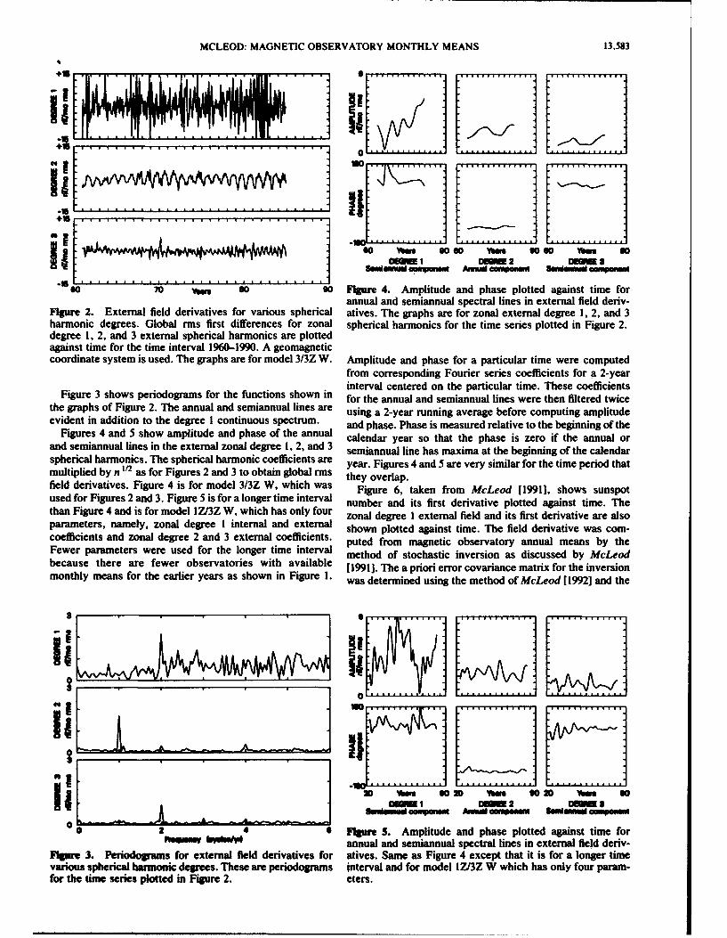
Figure 2. External field derivatives for various spherical atives. The graphs are for zonal external degree 1, 2, and 3harmonic degrees. Global rms first differences for zonal spherical harmonics for the time series plotted in Figure 2.degree 1, 2, and 3 external spherical harmonics are plottedagainst time for the time interval 1960-1990. A geomagneticcoordinate system is used. The graphs are for model 3/3Z W. Amplitude and phase for a particular time were computed

from corresponding Fourier series coefficients for a 2-yearinterval centered on the particular time. These coefficients

Figure 3 shows periodograms for the functions shown in for the annual and semiannual lines were then filtered twicethe graphs of Figure 2. The annual and semiannual lines are using a 2-year running average before computing amplitudeevident in addition to the degree 1 continuous spectrum. and phase. Phase is measured relative to the beginning of the

Figures 4 and 5 show amplitude and phase of the annual calendar year so that the phase is zero if the annual orand semiannual lines in the external zonal degree 1, 2, and 3 semiannual line has maxima at the beginning of the calendarspherical harmonics. The spherical harmonic coefficients are year. Figures 4 and 5 are very similar for the time period thatmultiplied by n1 12 as for Figures 2 and 3 to obtain global rms they overlap.field derivatives. Figure 4 is for model 3/3Z W, which was Figure 6, taken from McLeod [1991], shows sunspotused for Figures 2 and 3. Figure 5 is for a longer time interval number and its first derivative plotted against time. Thethan Figure 4 and is for model IZ/3Z W, which has only four zonal degree I external field and its first derivative are alsoparameters, namely, zonal degree I internal and external shown plotted against time. The field derivative was com-coefficients and zonal degree 2 and 3 external coefficients. puted from magnetic observatory annual means by theFewer parameters were used for the longer time interval method of stochastic inversion as discussed by McLeodbecause there are fewer observatories with available [1991]. The a priori error covariance matrix for the inversionmonthly means for the earlier years as shown in Figure 1. was determined using the method of McLeod [19921 and the

0

00 YOM___0__0______90_____VMSso

coMmi UI2 Oal3

0 2 4 6 Fiur S. Amplitude and phase plotted against time forFWWWAV kvannual and semiannual spectral lines in external field deriv-

Figure 3. Periodograms for external field derivatives for atives. Same as Figure 4 except that it is for a longer timevarious spherical harmonic degrees. These are periodograms interval and for model IZ/3Z W which has only four param-for the time series plotted in Figure 2. eters.


.. . . ..

A. AAA

02 4

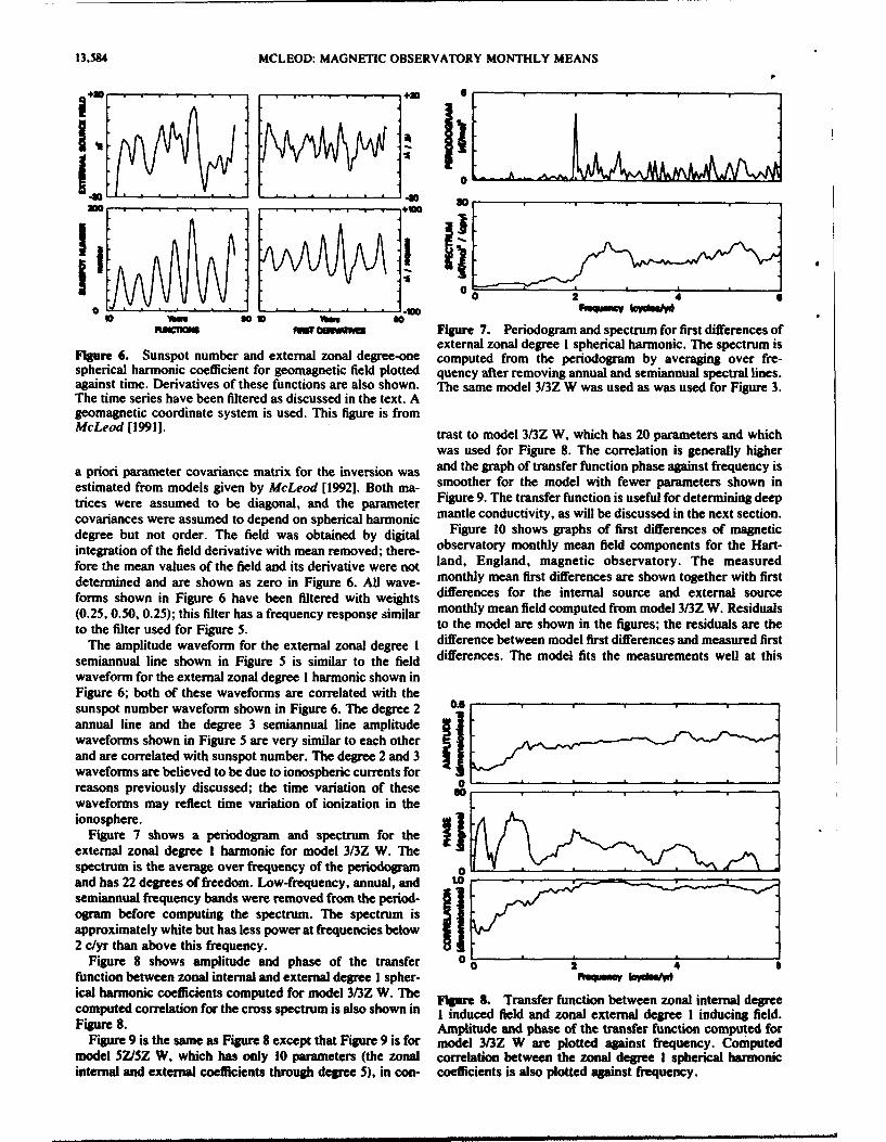
10 Ni 810sM so"mUdoI mtwr oawn Figure 7. Periodogram and spectrum for first differences of

external zonal degree 1 spherical harmonic. The spectrum isFigure 6. Sunspot number and external zonal degree-one computed from the periodogram by averaging over fre-spherical harmonic coefficient for geomagnetic field plotted quency after removing annual and semiannual spectral lines.against time. Derivatives of these functions are also shown. The same model 3/3Z W was used as was used for Figure 3.The time series have been filtered as discussed in the text. Ageomagnetic coordinate system is used. This figure is fromMcLeod [1991]. trast to model 3/3Z W, which has 20 parameters and which

was used for Figure 8. The correlation is generally higher

a priori parameter covariance matrix for the inversion was and the graph of transfer function phase against frequency is

estimated from models given by McLeod [1992]. Both ma- smoother for the model with fewer parameters shown in

trices were assumed to be diagonal, and the parameter Figure 9. The transfer function is useful for determining deep

covariances were assumed to depend on spherical harmonic mantle conductivity, as will be discussed in the next section.

degree but not order. The field was obtained by digital Figure 10 shows graphs of first differences of magnetic

integration of the field derivative with mean removed; there- observatory monthly mean field components for the Hart-

fore the mean values of the field and its derivative were not land, England, magnetic observatory. The measured

determined and are shown as zero in Figure 6. All wave- monthly mean first differences are shown together with first

forms shown in Figure 6 have been filtered with weights differences for the internal source and external source

(0.25, 0.50, 0.25); this filter has a frequency response similar monthly mean field computed from model 3/3Z W. Residuals

to the filter used for Figure 5. to the model are shown in the figures; the residuals are the

The amplitude waveform for the external zonal degree 1 difference between model first differences and measured first

semiannual line shown in Figure 5 is similar to the field differences. The model fits the measurements well at this

waveform for the external zonal degree I harmonic shown inFigure 6; both of these waveforms are correlated with thesunspot number waveform shown in Figure 6. The degree 2 0.5annual line and the degree 3 semiannual line amplitudewaveforms shown in Figure 5 are very similar to each otherand are correlated with sunspot number. The degree 2 and 3waveforms are believed to be due to ionospheric currents forreasons previously discussed; the time variation of these sowaveforms may reflect time variation of ionization in theionosphere. .

Figure 7 shows a periodogram and spectrum for theexternal zonal degree I harmonic for model 3/3Z W. Thespectrum is the average over frequency of the periodogram 0

and has 22 degrees of freedom. Low-frequency, annual, and Isemiannual frequency bands were removed from the period-ogram before computing the spectrum. The spectrum isapproximately white but has less power at frequencies below2 c/yr than above this frequency.

Figure 8 shows amplitude and phase of the transfer 0 2

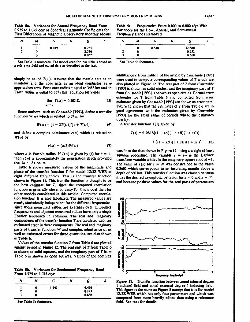
function between zonal internal and external degree 1 spher- k'qumy Ivoehuical harmonic coefficients computed for model 3/3Z W. The Figure 3. Transfer function between zonal internal degreecomputed correlation for the cross spectrum is also shown in I induced field and zonal external degree 1 inducing field.Figure 8. Amplitude and phase of the transfer function computed for

Figure 9 is the same as Figure 8 except that Figure 9 is for model 3/3Z W are plotted against frequency. Computedmodel 5Z/5Z W, which has only 10 parameters (the zonal correlation between the zonal degree I spherical harmonicinternal and external coefficients through degree 5), in con- coefficients is also plotted against frequency.


Similar outlier pairs are evident in graphs for other magneticobservatories (not shown) and are believed due to clericalerror in compiling the data sets. Similar outliers were found

in the annual mean data set used by McLeod [19921.An edited first difference data set was created from the

slightly edited first difference data set. This edited data setwas obtained by deleting all first differences from a given

4 observatory for any month in which any of the first differ-"ences for that observatory were judged to be outliers. Also,data from a few observatories were eliminated because those

0 _observatories had data for only a few months. About 3% ofto the first difference data were deleted in this manner to obtain

the edited first difference data set. The letter E is used in amodel name to indicate that the model was computed fromthe edited data set.

0 Table 4 is the same as Table 3 except that Table 4 is for0 2 4 6 model 3/3Z WE and Table 3 is for model 3/3Z W. All

variances for the continuous spectrum of Table 4 are lessthan corresponding variances of Table 3, except for the

FIgure 9. Transfer function between zonal internal degree zonal degree I variances. This observation is consistent withI induced field and zonal external degree 1 inducing field, the interpretation that the continuous spectrum variances ofThis figure is the same as Figure 8 except that it is for model Table 3, except for zonal degree I variances, are mostly due57J5Z W which has only 10 parameters. to noise in the data set caused by outliers; this noise is

reduced through use of the edited data set.

observatory. The model is found to be generally poor at A graph similar to Figure 9 was produced, except that thehigh-latitude observatories but good at midlatitude and low- transfer function was computed using the edited data set inlatitude observatories. place of the lightly edited data set used for Figure 9. The

The vertical magnetic field first differences shown in correlation function is generally closer to unity for the editedFigure 10 for the Hartland, England, magnetic observatory data than for the lightly edited data.exhibit a pair of outlying points at approximately 1983.5 in To reduce errors due to spatial aliasing by unmodeledboth measured data and residuals. These outliers are due to coefficients in the spherical harmonic analysis of first differ-a single outlier at approximately 1983.5 in the vertical ences of magnetic observatory monthly means, a referencemonthly means for Hartland. This single outlier produces an model for first differences of monthly means was created.outlier pair in the first differences of the monthly means. This reference model was created from the internal source

4 ........... ... .............. .............. ..............iiAJ JH H.......

so ybu W06o 0 bm W so Yew So 6o ThN go

Figure 10. First differences of Hartland, England, magnetic observatory monthly mean field compo-nents. Measured first differences for three field components are shown together with first differences ofexternal source and internal source monthly mean field computed from model 3/3Z W. Residuals to themodel are also shown; the residuals are the difference between model first differences and measured firstdifferences.


Table 4a. Variances for Annual Frequency Band From Table 4c. Variances for Frequencies From 0.000 to 6.0000.925 to 1.075 c/yr of Spherical Harmonic Coefficients for c/yr With Variances for the Low, Annual, and SemiannualFirst Differences of Magnetic Observatory Monthly Means Frequency Bands Removed


I 0 0.047 0.307 I 0 8.996 51.294I I 0.198 0.158 0.304 0.039 I I 0.967 0.956 0.499 0.5122 0 0.135 2.861 2 0 0.836 0.9682 I 0.059 0.118 2 I 0.563 0.5902 2 0.028 0.016 2 2 0.828 0.5123 0 0.116 0.035 3 0 0.589 0.7593 I 0.026 0.009 3 I 0.359 0.3453 2 0.048 0.017 3 2 0.487 0.3363 3 0.027 0.025 3 3 0.289 0.477

See Table 3a footnotes. The model used for this table is based on See Table 4a footnotes.edited data as described in the text.

reference model. Variances for the continuous spectrumportion of model 7/7Z W for first differences of annual means shown in Table 2c, except for the zonal degree I harmonics,described by McLeod [1992e. The annual means first differ- were also reduced for the new model.ence coefficients were filtered with weights (0.25, 0.50, 0.25) Additional models with various combinations of internaland used to compute filtered first difference coefficients for and external coefficient were produced. An expanded ver-monthly means by means of parabolic interpolation. First sion of this article that includes spectra and cross spectra fordifferences for the reference model were subtracted from the these models is available from the author. It was found thatmagnetic observatory first differences; spherical harmoo the best model for determining a transfer function betweencoefficients for the first difference residuals were then com- internal and external zonal degree 1 spherical harmonicptaed. The coefficients for the first difference residuals were coefficients was model IZ/3Z WER. Variances for this modelthen added to the coefficients for the reference field to tain are shown in Table 5. The transfer function is shown incoefficients for the monthly means. The model for the first Figure I11. This model was considered best for determining a

difference residuals was not generally of the same degree and transfer function, since the correlation shown in Figure a1

order as the reference model. When this method of analysis

is used, the coefficients of the reference model that are also was generally closer to unity for this model than for other

included in the residual model have no effect on the final models. Variances for the continuous spectrum, except for

result. This is because a change in these coefficients of the the zonal degree I harmonics, were generally smaller for this

reference model produces a corresponding change in the model than the other models.

residual model, so that the final sum model is unchanged.However, the coefficients of the reference model that are not Deep Mantle Conductivityincluded in the residual model can have a large effect on the Time-varying magnetic fields that originate from electricalfinal model. current systems external to Earth induce electrical currents

A model of degree and order 3 for both internal and within Earth. These induced currents in turn produce time-external spherical harmonics, model 3/3 WER, was pro- varying magnetic fields. The transfer function between in-duced from the edited data set using the reference model. duced and inducing spherical harmonic coefficients for aVariances were computed for this model and compared with given degree spherical harmonic can be used to studythose shown in Tables I and 2. It was found that external electrical conductivity of Earth as a function of depth.coefficient variances for the low-frequency band shown in Lateral homogeneity is assumed here as a reasonable ap-Table lb were greatly reduced for the new model. It was proximation so that the transfer function depends upon theconcluded that these external variances in Table lb ar degree but not the order of the spherical harmonic. Themostly due to spatial aliasing by unmodeled internal coeffi- transfer function also depends upon temporal frequency andcients and that this aliasing is greatly reduced by using the upon the conductivity profile of Earth.

If Earth is assumed to be an insulator for r > b and anideal conductor for r < b, then the transfer function between

Table 1b. Variances for Semiannual Frequency Band induced and inducing spherical harmonic coefficients isFrom 1.925 to 2.075 c/yr easily found from the boundary condition that the vertical

N M G H Q S field must be zero within the conductor. The transfer func-tion T.((o) for Schmidt seminormalized spherical harmonic

S0.098 0.093 0.125 0.019 coefficients is found to be2 0 0.027 0.124 n2 1 0.078 0.003 T,(wo) + - (b/a)2 +'+, (4)2 2 0.010 0.025 n3 0 0.062 0.8003 1 0.038 0.020 where n is the spherical harmonic degree, w = 22rf, f is3 2 0.019 0.024 temporal frequency, and a is Earth's radius.3 3 0.006 0.026 Induction only by degree 1 spherical harmonics will be

See Table 4a footnotes, considered in this section, and the transfer function will


Table S•. Variances for Annual Frequency Band From Table Sc. Frequencies From 0.000 to 6.000 c/yr With0.925 to 1.075 c/yr of Spherical Harmonic Coefficients for Variances for the Low, Annual, and SemiannualFirst Differences of Magnetic Observatory Monthly Means Frequency Bands Removed

N M G H Q S N U G H Q S

1 0 0.039 0.265 I 0 8.548 52.5802 0 2.536 2 0 0.5523 0 0.032 3 0 0.610

See Table 3a footnotes. The model used for this table is based on See Table 5a footnotes.a reference field and edited data as described in the text.

admittance c from Table I of the article by Constable [19931simply be called T(o). Assume that the mantle acts as an were used to compute corresponding values of T which areinsulator and the core acts as an ideal conductor as w also plotted in Figure 12. The real part of T from Constableapproaches zero. For a core radius c equal to 3485 km and an [19931 is shown as solid circles, and the imaginary part of TEarth radius a equal to 6371 kin, equation (4) yields from Constable [1993] is shown as open circles. Formal error

estimates for T from Table 6 and computed from errorlim T(wo) = 0.0818. (5) estimates given by Constable [1993] are shown as error bars.

00-+0 Figure 12 shows that the estimates of T from Table 6 are in

Some authors, such as Constable (19931, define a transfer good agreement with the estimates given by Constablefunction W((w) which is related to T(w) by [1993] for the small range of periods where the estimates

overlap.W(w) = [I - 2T(ow)]I[l + T(o)] (6) A transfer function T(s) given by

and define a complex admittance c(wo) which is related to T(s) = 0.0818[(l + sA)(I + sB)(i + sC)]W(w) by

[(I + sD)(l + sE)(I + sF)] (8)

O) = (al2)W(a,) (7)

was fit to the data shown in Figure 12, using a weighted leastwhere a is Earth's radius. If T(w) is given by (4) for n = I, squares procedure. The variable s = ih is the Laplacethen c(aw) is approximately the penetration depth provided transform variable while i is the imaginary square root of - I.that (a - b) << a. The value of T(s) for s = i- was constrained to the value

Table 6 shows measured values of the magnitude and 0.3602 which corresponds to an insulating mantle above aphase of the transfer function T for model IZ/3Z WER at depth of 660 km. This transfer function was chosen becauseeight different frequencies. This is the transfer function it has the desired asymptotic behavior for s = 0 and s = i®,shown in Figure 1i. This transfer function is thought to be and because positive values for the real parts of parametersthe best estimate for T, since the computed correlationfunction is generally closer •o unity for this model than forother models considered in this article. Computed correla-tion function R is also tabulated. The measured values are o.5nearly statistically independent for the different frequencies, Msince these measured values are averages over I I Fourierfrequencies and adjacent measured values have only a singleFourier frequency in common. The real and imaginarycomponents of the transfer function T are tabulated with the oestimated error in these components. The real and imaginary soparts of transfer function W and complex admittance c, aswell as estimated errors for these quantities, are also shownin Table 6. t

Values of the transfer function T from Table 6 are plotted 0 _fill,

against period in Figure 12. The real part of T from Table 6 ois shown as solid squares, and the imaginary part of T fromTable 6 is shown as open squares. Values of the complex

Table Sb. Variances for Semiannual Frequency Band o _o_ ___ ___ ___

From 1.925 to 2.075 c/yr 2

N M G H Q S Figure 11. Transfer function between zonal internal degreeI induced field and zonal external degree I inducing field.2 0 1.945 6.492 This figure is the same as Figure 8 except that it is for model2 0 0. 173

3 0 0.638 IZ/3Z WER which has only four parameters and which wascomputed from more heavily edited data using a reference

See Table 5a footnotes. field. See text for details.


S.a.

IIII_ __I_ II_ _ _

.12

£" "d i ...... il .. . I

0 .; C; E Figure 12. Complex transfer function (T) plotted against

W) " period. Solid squares are the real part of T, and open squaresare the imaginary part of T as determined in this study andtabulated in Table 6. Solid circles are the real part of T, and

"-• -. open circles are the imaginary part of T as computed from"" CS CS .. .. data given by Constable [19931. The solid and dashed curves

" •are the real and imaginary part of T, respectively, computed-- from equation (8).

" .D, E, and F are sufficient to ensure that the transfer function-• •satisfies causality. The best fit was found for time constants

W81 0 .2 A = 0.4399 year, B = 0.02926 year, C = 0.004079 year,0 (6 C D = 0.1479 year, E - 0.02287 year, F = 0.003529 year.

. 5S IThe real and imaginary parts of this transfer function areC-.9 .plotted in Figure 12 as solid and dashed curves, respectively.

oI lI The transfer function T(s) given by (8) can be expanded as

X- s -T(s) = 0.0818 + asDI(1 + sD) + PsE/(1 + sE)

ti 4 r4 % Z.* + ysFI(1 + sF), (9)

• .a. where the time constants D, E, and F have the same values.2 as for (8) and the constants a, P, and y are a = 0.1527, P

- 0.0741, and y = 0.0513.

-ý ,The response of T(s) to a unit step function in the externalZ j= field Et) at t = 0 is the internal field l(t) given by

I(t) = 0.0818 + 0.1527 exp (-t/D) + 0.0741 exp (-tIE)

-+ ~ 0.0513 exp (-tIF) (10)

Z8 where t is time and D, E, and F have the same values as for. ,... • (8). E(t) is the magnitude of the uniform external field and

1(t) is the magnitude of the induced dipole field at the- - geomagnetic equator. Equation (10) is valid for t > 0; 1(t)

0 fort < 0. In units of days, the time constants areD = 54.0days, E=8.4 days, andF= 1.29 days.

S• Equation (10) is applicable for a superconducting core anda mantle that is an insulator above a depth of 660 kin. SinceSthe core is not a superconductor, the constant term 0.0818 in(10) should be expected to decay with a time constant of a

C4 fn 'W % % r. 00 few thousand years. Since the mantle above 660 km is not anz insulator, an additional term should be included in (10). lhe

"MCLEOD: MAGNETIC OBSERVATORY MONTHLY MEANS 13,589

additional term is approximately 0.1401 exp (- t/G), where Estimation of the global response function at frequenciesG is of the order of I hour. The coefficient 0.1401 in the less than 2 c/yr is subject to larger relative errors thanadditional term ensures that (0 + ) = 0.5, in agreement with estimation of the response at higher frequencies, for several(4), where 0+ indicates a limit as t approaches 0 from the reasons. First, the power spectral density of the externalright, source signal is less below 2 c/yr than above this frequency.

Second, the induced internal source signal is smaller relativeto the inducing signal at the lower frequencies. Third,

Condusions possible error sources, such as core source signals that areFirst differences of magnetic observatory monthly means not due to induction and ionospheric source signals that are

for years 1963-1982 have been analyzed using techniques of not modeled by the spherical harmonic analysis, can reason-spherical harmonic analysis and power spectral analysis. ably be expected to be larger at low frequencies; in particu-Except for Earth's auroral regions, the external source lar, ionospheric signals at the sunspot frequency and itssignal is primarily zonal in geomagnetic coordinates. The harmonics can be expected. Nevertheless, improvements tospectrum of the external source signal consists of lines at 1 the estimate for the global response function may be possibleand 2 c/yr superimposed on a continuous spectrum. The by using more recent observatory data than is available fromcontinuous spectrum is well represented by zonal degree I the National Geophysics Data Center on the compact diskspherical harmonics. The annual spectral line is primarily NGDCO1. Also, it may be possible to obtain observatoryzonal degree 2; however, the annual line also includes small data not presently available from the National Geophysicsbut significant spherical harmonics of other degrees and Data Center. Using a longer time interval could possiblyorders. The semiannual line is primarily zonal degree 1 but result in some improvement, although the data quality is notincludes a significant zonal degree 3 harmonic, as well as as good for years prior to the time interval used for thissmaller harmonics of other degrees and orders. The non- study.degree I harmonics and part of the degree I harmonic for the Although the response function found here agrees wellannual and semiannual line spectra are due to ionospheric with the response for the conductivity profile proposed bycurrent systems. The continuous spectrum for the frequency Banks [1969], as discussed by Achache et al. [19811, therange studied is due primarily to the ring current and question of uniqueness of the conductivity profile compati-magnetopause currents, except for the auroral regions where ble with the estimated response function has not beenionospheric currents dominate, explored in depth and is beyond the scope of this article.

The continuous spectrum, with annual and semiannual Some scientists have proposed a very thin, highly con-spectral lines excluded, has been used in this paper to ducting layer in the mantle adjacent to the core-mantleestimate a global geomagnetic response function for periods boundary. Such a layer is compatible with the estimatedranging from 2 months to 2 years and sensitive to average response, since such a layer would have the same smallradial electrical conductivity of the deep mantle down to the effect on the global response as a small increase in thecore-mantle boundary. The estimated response function core radius. Investigation of the existence of such a thinfound here agrees well with the values given by Constable layer appears to require use of signals originating within[1993] for the narrow range of frequencies where the esti- the core, such as geomagnetic jerks. The sharpness of themates overlap. The response function found here also agrees jerks observed at many observatories appears to bewell with the value found by McLeod [1992] for a 2-year compatible with the time constants found here for the globalperiod and with the response for the conductivity profile response function; nevertheless, further research on thisproposed by Banks [1969] as described by Achache et al. subject is desirable.[ 1981 ] for which conductivity at the core-mantle boundary isabout 10 S/m. Note added in proof. The transfer function W(s) corre-

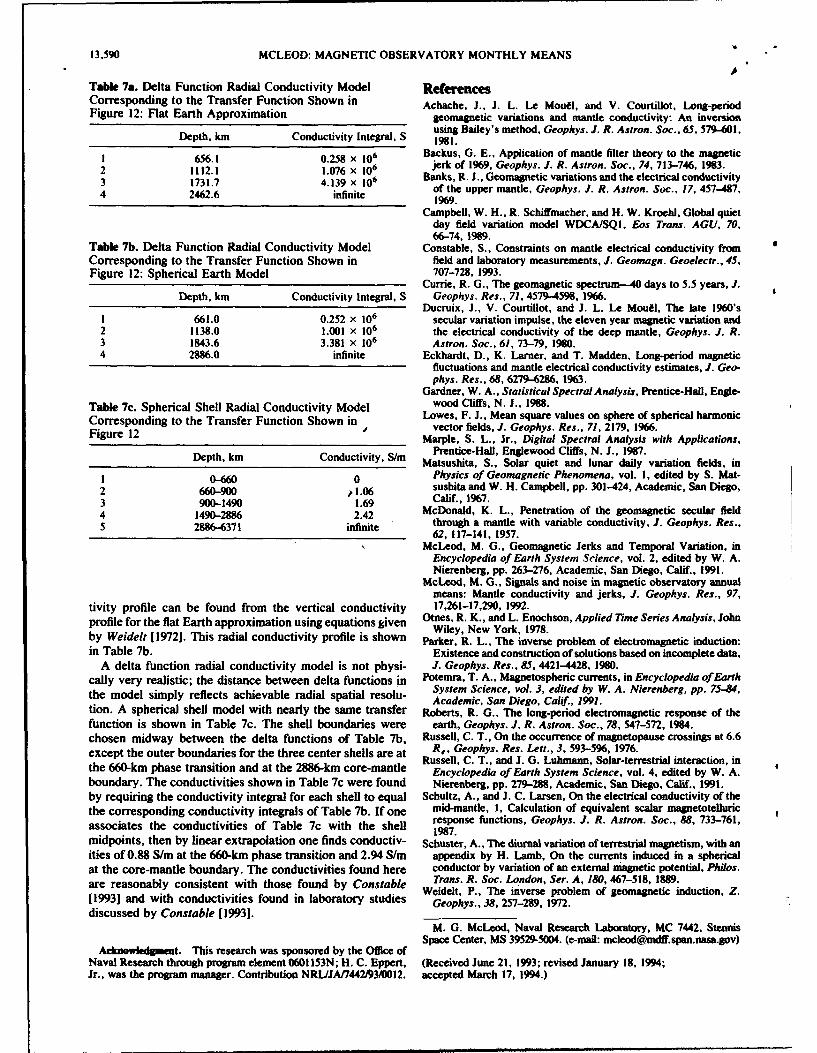
Because the continuous spectrum is primarily zonal sponding to T(s) given by equation (8) is, using equation (6),degree 1, this spectrum is well suited for estimation of aglobal geomagnetic response function. Neither the annual W(s) = 0.773[(1 + sa)(l + sb)(1 + sc)]nor semiannual spectral lines are due to a single sphericalharmonic. The annual line is mainly due to ionospheric + [(1 + sd)(l + se)(l + sf)] (11)currents, while the semiannual line contains a significantcontribution from ionospheric currents. Since neither line with time constants a = 0.09691 year, b = 0.01637 year,can be modeled as well as the continuous spectrum c = 0.002521 year, d = 0.1690 year, e = 0.02422 year,using available magnetic observatory monthly means, f = 0.003665 year. The admittance function c(s) is W(s)these lines are not well suited for estimation of a global multiplied by 3186 km. Weidelt [1972] and Parker [19801geomagnetic response function. Attempts by some pre- have discussed admittance functions of this type withvious investigators to use these lines, particularly the semi- interlaced real poles and zeros. For a flat Earth approxi-annual line, have resulted in large errors in estimates of mation, the vertical conductivity profile is a finite comb ofthe global response function at these frequencies, as is positive delta functions. Parker [1980] has shown thatapparent in graphs of measured global response function the depths and magnitudes of these delta functions can beshown by Achache et al. [1981]. A further advantage to found from a continued fraction expansion of the admittanceusing the continuous spectrum for estimating a global function. The depths and conductivity integrals for the deltaresponse function is that this method permits estimation function vertical conductivity profile corresponding to equa-of correlation between internal and external source signals; tion (11) for the flat Earth approximation is shown in Tablethus errors in the estimated response function can readily 7a. The radial conductivity profile for a spherical Earthbe estimated, model also consists of delta functions. This radial conduc-


Table 7a. Delta Function Radial Conductivity Model ReferencesCorresponding to the Transfer Function Shown in Achache, J., J. L. Le Mouel, and V. Courtillot, Long-periodFigure 12: Flat Earth Approximation geomagnetic variations and mantle conductivity: An inversion

using Bailey's method, Geophys. J. R. Astron. Soc., 65,579-601,Depth, km Conductivity Integral, S 1981.

! 656.1 0.258 x 106 Backus, G. E., Application of mantle filter theory to the magnetic

2 1112.1 1.076 X 106 jerk of 1969, Geophys. J. R. Astron. Soc., 74, 713-746, 1983.

3 1731.7 4.139 x 106 Banks, R. J., Geomagnetic variations and the electrical conductivityof the upper mantle, Geophys, J. R. Astron. Soc., 17, 457-487,

4 2462.6 infinite 1969.

Campbell, W. H., R. Schiffmacher, and H. W. Kroehl, Global quietday field variation model WDCA/SQI, Eos Trans. AGU, 70,66-74, 1989.

Table 7b. Delta Function Radial Conductivity Model Constable, S., Constraints on mantle electrical conductivity fromCorresponding to the Transfer Function Shown in field and laboratory measurements, J. Geomagn. Geoelectr., 45,Figure 12: Spherical Earth Model 707-728, 1993.

Currie, R. G., The geomagnetic spectrum-40 days to 5.5 years, J.Depth, km Conductivity Integral, S Geophys. Res., 71, 4579-4598, 1966.

Ducruix, J., V. Courtillot, and J. L. Le Mouel, The late 1960's1 661.0 0.252 x 106 secular variation impulse, the eleven year magnetic variation and2 1138.0 1.001 X 106 the electrical conductivity of the deep mantle, Geophys. J. R.3 1843.6 3.381 x 106 Astron. Soc., 61, 73-79, 1980.4 2886.0 infinite Eckhardt, D., K. Lamer, and T. Madden, Long-period magnetic

fluctuations and mantle electrical conductivity estimates, J. Geo-phys. Res., 68, 6279-6286, 1963.

Gardner, W. A., Statistical Spectral Analysis, Prentice-Hall, Engle-Table 7c. Spherical Shell Radial Conductivity Model wood Cliffs, N. J., 1988.Corresponding to the Transfer Function Shown in Lowes, F. J., Mean square values on sphere of spherical harmonicFigure 12 vector fields, J. Geophys. Res., 71, 2179, 1966.Marple, S. L., Jr., Digital Spectral Analysis with Applications,

Depth, km Conductivity, S/in Prentice-Hall, Englewood Cliffs, N. J., 1987.Depth,____ _Conductivity,__ S/ Matsushita, S., Solar quiet and lunar daily variation fields, in

1 0-660 0 Physics of Geomagnetic Phenomena, vol. I, edited by S. Mat-2 660-900 , 1.06 sushita and W. H. Campbell, pp. 301-424, Academic, San Diego,3 900-1490 1.69 Calif., 1967.4 1490-2886 2.42 McDonald, K. L., Penetration of the geomagnetic secular field5 2886-6371 infinite through a mantle with variable conductivity, J. Geophys. Res.,

62, 117-141, 1957.McLeod, M. G., Geomagnetic Jerks and Temporal Variation, in

Encyclopedia of Earth System Science, vol. 2, edited by W. A.Nierenberg, pp. 263-276, Academic, San Diego, Calif., 1991.

McLeod, M. G., Signals and noise in magnetic observatory annualmeans: Mantle conductivity and jerks, J. Geophys. Res., 97,

tivity profile can be found from the vertical conductivity 17,261-17,290, 1992.profile for the flat Earth approximation using equations given Otnes, R. K., and L. Enochson, Applied Time Series Analysis, John

Wiley, New York, 1978.by Weidelt [1972]. This radial conductivity profile is shown Parker, R. L., The inverse problem of electromagnetic induction:in Table T7. Existence and construction of solutions based on incomplete data,

A delta function radial conductivity model is not physi- J. Geophys. Res., 85, 4421-4428, 1980.cally very realistic; the distance between delta functions in Potemra, T. A., Magnetospheric currents, in Encyclopedia of Earth

System Science, vol. 3, edited by W. A. Nierenberg, pp. 75-84,the model simply reflects achievable radial spatial resolu- Academic, San Diego, Calif., 1991.tion. A spherical shell model with nearly the same transfer Roberts, R. G., The long-period electromagnetic response of thefunction is shown in Table 7c. The shell boundaries were earth, Geophys. J. R. Astron. Soc., 78, 547-572, 1984.chosen midway between the delta functions of Table 7b, Russell, C. T., On the occurrence of magnetopause crossings at 6.6except the outer boundaries for the three center shells are at R,, Geophys. Res. Lett., 3, 593-596, 1976.

Russell, C. T., and J. G. Luhmann, Solar-terrestrial interaction, inthe 660-km phase transition and at the 2886-km core-mantle Encyclopedia of Earth System Science, vol. 4, edited by W. A.boundary. The conductivities shown in Table 7c were found Nierenberg, pp. 279-288, Academic, San Diego, Calif., 1991.by requiring the conductivity integral for each shell to equal Schultz, A., and J. C. Larsen, On the electrical conductivity of thethe corresponding conductivity integrals of Table 7b. If one mid-mantle, I, Calculation of equivalent scalar magnetotelluricassociates the conductivities of Table 7c with the shell response functions, Geophys. J. R. Astron. Soc., 88, 733-761,

1987.midpoints, then by linear extrapolation one finds conductiv- Schuster, A., The diurnal variation of terrestrial magnetism, with anities of 0.88 S/m at the 660-km phase transition and 2.94 S/m appendix by H. Lamb, On the currents induced in a sphericalat the core-mantle boundary. The conductivities found here conductor by variation of an external magnetic potential, Philos.are reasonably consistent with those found by Constable Trans. R. Soc. London, Ser. A, 180, 467-518, 1889.

Weidelt, P., The inverse problem of geomagnetic induction, Z.[1993] and with conductivities found in laboratory studies Geophys., 38, 257-289, 1972.discussed by Constable [1993].

M. G. McLeod, Naval Research Laboratory, MC 7442, StennisSpace Center, MS 39529-5004. (e-mail: [email protected])

Acknowledgment. This research was sponsored by the Office ofNaval Research through program element 0601153N; H. C. Eppert, (Received June 21, 1993; revised January 18, 1994;Jr., was the program manager. Contribution NRL/JAf7442/93/0012. accepted March 17, 1994.)

rs ' oftumentation pagefomave ad- a283 368

Documents