ROTATION CURVES OF GALAXIES

A project report submitted in partial fulfilment

for the award of the Masters degree in Physics

by

PARVATHY HARIKUMAR

Reg.no.34313011

under the guidance of

Dr. L. Sriramkumar

Department of Physics

Indian Institute of Technology Madras

Department of Theoretical Physics

University of Madras

Maraimalai Campus, Guindy

Chennai-600 025

May 2015

1

CERTIFICATE

This is to certify that the project entitled Rotation curves of galaxies submitted by

Parvathy Harikumar, in partial fulfilment for the award of Masters degree in Physics,

is an independent bona fide record of work done by the candidate at University of

Madras.

(L. Sriramkumar, Project supervisor)

2

Acknowledgement

I’m greatly indebted to Dr. L. Sriramkumar, Associate Professor, Department of

Physics, Indian Institute of Technology, Madras, for being an honest critique and a strict

mentor and for giving me an unparalleled guidance throughout the course of this project.

I would like to thank Dr. Ranabir Chakrabarti, Head of the department, Department of

Theoretical Physics, University of Madras, for providing me with this opportunity. I

express my sincere gratitude to Dr. Vytheeswaran, Assistant Professor, Department

of Theoretical Physics, University of Madras, for his valuable insights on the subject.

I would also like to thank Dr. R. Radhakrishnan, Assistant Professor, Department of

Theoretical Physics, University of Madras, for taking a sincere effort to help me tackle

problems in the due course.

It is hard to conclude without mentioning the names of my friends who helped me

in every way possible in completing this project. First of all, I thank my classmates and

the PhD scholars of my department for their support. I would like to specially thank

my friend Mr. Arjun for his peerless motivation and valuable suggestions. I thank my

friends Ms. S. Brinda and Ms. R. Anubama for inspiring me to work independently

with immense dedication and passion.

I don’t have words to express my gratitude and love to those who matter the most,

my parents. They are the reason why I’m here and they are the only people who have

always been with me through thick and thin.

3

Abstract

Understanding the complex working of our universe relies partially on understand-

ing the dynamics of self gravitating systems like galaxies and globular clusters which

form an integral part of the universe. Since the components that make up such systems

move in their orbits at non relativistic velocities, a Newtonian approach can very well

be adopted to study them. In this report, the gravitational potential arising due to the

distribution of mass in a galaxy is obtained from the distribution function frozen at a

point of time in the phase space. Our aim is to assign a suitable form of density profile

to the distribution of dark matter in galaxies such that the flat rotation curves,obtained

from the studies of motion of stars and clouds, is reproduced. To get a deeper idea of

the concept, we shall also look at how the orbits of stars and their respective orbital

periods are determined theoretically.

4

TABLE OF CONTENTS

1 Introduction 6

2 Gravitational dynamics 8

2.1 An overview of self gravitating systems . . . . . . . . . . . . . . . 8

2.2 Collisionless boltzmann equation . . . . . . . . . . . . . . . . . . . 9

2.2.1 Models of Galaxies . . . . . . . . . . . . . . . . . . . . . . 11

3 Orbits of stars 25

3.1 Orbits in spherically symmetric potentials . . . . . . . . . . . . . . 25

3.2 Rotation curves of galaxies . . . . . . . . . . . . . . . . . . . . . . 30

3.2.1 Orbits in axisymmetric systems . . . . . . . . . . . . . . . 32

3.2.2 Evidence for the existence of dark matter . . . . . . . . . . 36

4 Conclusion 39

5

CHAPTER 1

Introduction

”The innocent and light minded, who believe that astronomy can be studied by looking

at the heavens without knowledge of mathematics, will return in the next life as birds.”

-Plato

The best thing about the dark night sky which blankets half the earth is that half of us

can see those beautiful glimmering gems scattered against the black canvas, and if you

take a moment to step outside you too can marvel this small glimpse of the universe

beyond. The stars that we see do not individually make up the Universe but are all

bound by a universal force called gravity, the very reason why the apple fell on Newtons

head. He was the first Scientist to understand the role gravity plays in explaining why

everything is the way it is like and why Earth and all other planets revolve around

the Sun in nearly elliptical orbits. This was a breakthrough in the history of Science

as it paved its way to many inventions like rockets, satellites and space stations when

we learned what kept us here and we gradually figured out how to escape its effects

using sufficient velocity called the escape velocity. A galaxy is formed through many

stages of evolution commencing from a huge clump of gas clouds collapsing under its

own gravity to form what we see now. In most cases, in the centre of a galaxy dwells

a supermassive black hole whose enormous gravity has an inimitable impact on the

dynamics of its parent galaxy.

The prodigiousness of gravity lies in the fact that the same force which keeps our

feet on the ground can suck in the matter from a star as huge as our Sun to form an

accretion disk around a black hole. Most of the dynamics of stars, galaxies and clusters

of galaxies can be understood with the Newtonian concept of gravity as the subjects are

macroscopic objects.

Centuries ago, when the galaxies were only being discovered one by one, they were

thought to be island universes isolated from each other. But only later on did Scientists

find that it is not so. Galaxies do interact among their neighbouring galaxies through

gravitational forces and just like how the rotation of moon around the Earth cause waves

in the ocean, the gravitational field of a galaxy has tidal effects on other galaxies. Many

factors influence the formation and evolution of galaxies as a consequence of which we

observe different structures in them. Structure simply implies the way stars and other

components are distributed in space. Sometimes they are distributed on a disk like

structure embedded in a spherical halo whereas in other cases they might be distributed

in a spiral or elliptical shape and it goes on. Our focus will be primarily on the former

distribution of stars. As we all know dark matter makes up most of the universe. But

it interacts very weakly with ordinary matter. Out of the four fundamental forces in

nature, dark matter is believed only to exert a gravitational force on matter. Anything

non luminous and occupying a significant volume in a galaxy is nothing but dark matter.

The distribution of dark matter can be understood from what we call the rotation curves

of galaxies. Once we discuss the aspects of the self consistency of the distribution

function of stars in a galaxy in the second chapter, we will go on to this simple but

interesting idea of how dark matter has an influence of the orbital velocity of the stars in

the spherical halo. The basic intention of this report is to find the rotation curves of disk

galaxies embedded in a spherical halo consisting of old stars and dark matter starting

from the description of such systems by the Collisionless Boltzmann equation(CBE).

7

CHAPTER 2

Gravitational dynamics

2.1 An overview of self gravitating systems

Gravity is a force we are all familiar with. In fact we take it for granted even when

its profound effects permeates through matter and every cell in our body. According

to Einstein, mass of an object attributes to its gravity and that bends the space time

surrounding it. In a Galaxy, the stars move under the influence of the gravitational

field due to the stars in the background. Such systems are generally termed as self

gravitating systems as they evolve in a field created by the mass of the entire galaxy

to which it contributes its share. Because of self-gravity, stellar systems have to face a

natural tendency to collapse. In the absence of dissipation, one may assume equilibrium

configurations in which random motions are able to oppose the tendency to collapse.

In this chapter, a close analogy is drawn between such systems and a barotropic fluid

whose density is a function of pressure of the fluid and vice versa. This assumption will

become clear as we go further.

Though everything looks fair enough in this context, unlike in fluids where the

molecules (gas or liquid) collide with each other on their path and approach a Maxwellian

distribution to achieve a thermal equilibrium, here we assume Galaxies to have reached

their steady state configuration. This follows from the fact that all Galaxies that we

see have formed billions of years ago. In just the same way as a gas kept in a container

comes into equilibrium with the surroundings on leaving it for an ample amount of time,

a Galaxy also forms and evolves through different stages to be what they look like now.

Moreover Galaxies are assumed to be a collisionless system of stars with a relaxation

time much larger than the age of the universe itself. Though close encounters between

stars have been reported, we have never witnessed a head on collision among stars.

As we all know, stars are formed from a gas cloud comprised of mostly Hydro-

gen and Helium, but the temperatures developed as a result of the exothermic nuclear

fusion ionises the gas and hence form plasma. Thus inside a star, other than the gravi-

tational forces that keeps the components together there is equally an electrostatic force

of attraction or repulsion between the charged ions of the plasma.

2.2 Collisionless boltzmann equation

One of the many crude approximations to study the self gravitating systems is that they

are in more or less a steady state. Though evolution is inevitable, stellar systems may

be treated as if they are in a thermal equilibrium for the time domain in which they are

studied. If we think of the gravitational potential of the galaxy as the sum of a smoothly

varying averaged component and a steep potential well near each star,the situation gets

more complicated to handle(see figure.2.1) [10].

In the beginning of the chapter we had discussed why the constituent particles

should evolve in a collisionless manner. In much the same way we can also discuss

why the velocity of these particles should approach a Maxwellian distribution in the

process of attaining a thermal equilibrium. Rather than thinking of stars as localised

point particles in a galaxy,it is more appropriate to treat them as a fluid smoothly dis-

tributed from one end to the other. Thus, we can introduce a distribution function f(x,v,t)

that gives the number of stars in a phase space volume d3xd3v at time t assuming stars

to move in phase space. So the probability of finding it at any given phase-space loca-

tion evolves with time. In fluid flow,mass of fluid passing a boundary is conserved as

long there are no sources and sinks. So the conservation of fluid mass described by the

continuity equation in fluid dynamics for a fluid of density ρ and velocity x is given by,

∂ρ

∂t+

∂

∂x(ρx) = 0 (2.1)

In our assumption, stars do have a lifetime after which they die and new stars are

9

Figure.2.1.(a)Smooth potential,(b)Potential wells near each star

born in the gas clouds of Galaxies. But if the rate of birth of stars, say B and rate of

death of stars say D is nearly equal,then B-D ≈0. For an evolving system of stars, if C

denotes the collision terms (df/dt) = C. [1] wherein assuming a collisionless evolution

we get the Boltzmann equation.df

dt= 0 (2.2)

Expanding out the time derivative and using v = −∇Φ, we can express the equations

that describe a collisionless gravitating system as

df

dt=∂f

∂x+ v.

∂f

∂v+ x.

∂f

∂x=∂f

∂t+ v.

∂f

∂x−∇Φ.

∂f

∂v= 0 (2.3)

with the potential determined by

∇2Φ = 4πGρ, ρ(x, t) = m

∫f(x, v, t)d3v (2.4)

This is the collisionless Boltzmann equation which is a special case of Liouville’s theo-

rem. It states that the flow of stellar phase points through phase space is incompressible,

or the phase space density around the phase point of any star remains constant.

Depending on the distribution function which is different for different stellar sys-

tems a wide variety of solutions are obtained to the coupled equations eqn(2.3) giving

rise to many possible models for galaxies which will be discussed in detail in the next

section. As of now we limit our discussions to the time independent solutions to the

equations where f(t, x, v) = f(x, v). We know from the definition of an integral of

10

motion that a function in phase space coordinates is an integral only if

dI(x,v)

dt= 0 (2.5)

For stars moving in the stationary potential Φ, let Ii, i = 1, 2.. be a set of integrals,

which is right now unknown. It is obvious that any function f(Ii) of the I ′is will satisfy

the steady-state Boltzmann equation;(df/dt) = (∂f/∂Ii)Ii = 0,as Ii is identically

zero [1]. If we can now determine the Φ from from f self-consistently and populate the

orbits of Φ with stars, we have solved the problem.

For the ease of calculations, we will first look at models in which the density and

the potential are spherically symmetric. Also it is convenient to shift the origin of Φ

by defining a relative potential Ψ ≡ −Φ + Φ0, where Φ0 is a constant. This potential

satisfies the equation

∇2Ψ = −4πGρ (2.6)

and the boundary condition Ψ → Φ0 as |x| → ∞.. We also define a shifted energy for

particles ε = −E+Φ0; because Φ0 = Ψ+Φ, ε = −E+Ψ+Φ = −12v2 +Ψ. Sometimes

distribution function depends only on the energy ε. Such models of galaxies are known

as Isotropic models. In other cases it depends on both energy and angular momentum

Lz and are known as Anisotropic models. These models are discussed in greater detail

in the next section.

2.2.1 Models of Galaxies

Isotropic models

In any steady-state potential Φ(x), the Hamiltonian H is an integral of motion. Con-

sequently, an equilibrium stellar system is obtained by taking f to be any non-negative

function of the Hamiltonian. Distribution functions of this type are called ergodic as

every state has a large finite probability to recur. If the potential is constant in an iner-

tial frame, H will be of the form H = 12v2 + Φ(x) and it follows that velocity vanishes

11

everywhere:¯ν(x) =

1

ν(x)

∫d3vvf(

1

2v2 + Φ(x)) = 0 (2.7)

where the second equality follows because the integrand is an odd function of v and the

integral is over all velocity space. A similar line of reasoning shows that the velocity-

dispersion tensor is isotropic:

σ2ij = vivj = σ2δij (2.8)

σ2(x) =1

ν(x)

∫dvzv

2z

∫dvydvxf(

1

2(v2x + v2

y + v2z) + Φ(x))

=4π

3ν(x)

∫ ∞0

dvv4f(1

2v2 + Φ). (2.9)

Hence, f(x, v) = f(ε) = f(Ψ− 12v2). The density ρ(x) corresponding to this distribu-

tion is

ρ(x) =

∫ √2Ψ

0

4πv2dvf(Ψ− 1

2v2) =

∫ Ψ

0

4πdεf(ε)√

2(Ψ− ε) (2.10)

As we are concerned only about the particles bound in the system’s potential, the limits

of the integral are the values that the potential takes at the boundaries. Once f is spec-

ified the right hand side becomes a known function of Ψ from which density ρ can be

determined using the Poisson’s equation. For a spherically symmetric potential,

1

r2

d

dr(r2dΨ

dr) = −4πG = −16π2G

∫ Ψ

0

dεf(ε)√

2(Ψ− ε) (2.11)

From the above equation,Ψ(r) can be obtained with some central value Ψ(0) and the

boundary conditions Ψ′(0) = 0. Once Ψ(r) is known, all other variables can be com-

puted.

It is quite straightforward to find a relation between a given density ρ(r) and the

unique f(ε) generated by it. This is done primarily by determining Ψ(r) from ρ(r) and

12

eliminating r which gives from eqn(2.11) ,

1√8πρ(Ψ) = 2

∫ Ψ

0

f(ε)√

Ψ− ε (2.12)

And differentiating both sides with respect to Ψ, we get

1√8π

dρ

dΨ=

∫ Ψ

0

f(ε)dε√Ψ− ε

. (2.13)

This equation is known as the Abel’s integral equation [2] and has the solution,

f(ε) =1√8π2

d

dε

∫ ε

0

(dρ

dΨ

)dΨ√ε−Ψ

, (2.14)

which determines f(ε). Depending upon the choice of f(ε),we can classify spherically

symmetric models into three classes of models which are namely the singular isothermal

sphere and the Kings model.

The simplest form of the distribution function is a power law with f(ε) = Aεn−32

for ε > 0 and zero otherwise.Using equation (2.12),we get

1√8πρ(ϕ) = 2

∫ ϕ

0

Aεn−32√ϕ− εdε (2.15)

To solve the above integral, it is appropriate to make use of the Walli’s formula given

by,

2

∫ 1

0

√1− x2dx = Γ(

1

2)Γ(

3

2) (2.16)

On substituting x2 = t in the formula, we get

2

∫ 1

0

t12−1(1− t) 3

2−1

2dt = Γ(

1

2)Γ(

3

2) (2.17)

In general for some α and γ, it becomes the famous Euler-Beta integral [9],

∫ 1

0

tα−1(1− t)β−1dt =Γ(α)Γ(β)

Γ(α + β)(2.18)

13

The equation(2.15)can also be written as,

1√8πρ(ϕ) = 2

∫ ϕ

0

Aε(n−12

)−1√ϕ(1− ε

ϕ)32−1dε

On multiplying and dividing by ϕ(n− 12−1), we get

2

∫ ϕ

0

Aε(n−12

)−1√ϕ(1− ε

ϕ)32−1dε = 2

∫ 1

0

Aε

ϕ

(n− 12

)−1

ϕn(1− ε

ϕ)( 3

2− 1)

dε

ϕ

(2.19)

On substituting (ε/ϕ) = t in eqn(2.19) and comparing it with eqn(2.18) we get α =

n− 12and β = 3

2,which gives

1√8πρ(ϕ) = 2Aϕn

Γ(n− 12)Γ(3

2)

Γ(n− 12

+ 32)

(2.20)

Using the properties of Gamma functions, we obtain the density as a function of the

potential to be

ρ(ϕ) = 2√

2πAϕnΓ(n− 1

2)√π

Γ(n+ 1)

= Bϕn,

(2.21)

where

B = (2π)32A

Γ(n− 12)

Γ(n+ 1)(2.22)

f(ε) =ρ0

(2πσ2)32

exp(ε

σ2) (2.23)

where ρ0 and σ are constants

Isothermal sphere

The Isothermal sphere is a configuration of infinite radius and infinite mass. We

know that for barotropic fluids, the pressure P is dependent on the density ρ of the

14

fluid. When P ∝ ρ, we get an isothermal sphere. Now, it can be shown easily that the

following distribution function describes an isothermal sphere,

f(ε) =ρ0

(2πσ2)32

exp(ε

σ2), (2.24)

which is parametrized by two constants ρ0 and σ. The distribution of velocities at

each point in the stellar isothermal sphere is the Maxwellian or Maxwell-Boltzmann

distribution. Thus the mean square speed of stars at a point is given by,

〈v2〉 =

∫∞0dvv4 exp(

ϕ− 12v2

σ2 )∫∞0dvv2 exp(

ϕ− 12v2

σ2 )

By eliminating exp( ϕσ2 ) and substituting v2

2σ2 = x2 ⇒ v =√

2σx, we get

〈v2〉 = 2σ2

∫∞0x4 exp(−x2)dx∫∞

0x2 exp(−x2)dx

Making use of the Gamma integral [9],

∫ ∞0

xm exp(−ax2)dx =Γ(m+1

2)

2am+1

2

(2.25)

the equation becomes,

〈v2〉 =2σ2 3

2Γ(3

2)

Γ(32)

= 3σ2

(2.26)

It is quite straightforward to find the density ρ(r) from f(ε),

ρ(r) =

∫ ϕ

0

4πdεf(ε)√

2(ϕ− ε)

=2ρ0√πσ2

exp(ϕ

σ2)

∫ ∞0

exp(−(ϕ− ε)

σ2)

√2(ϕ− ε)σ2

dε

(2.27)

15

On substituting (ϕ− ε)/σ2 = x and using the Gamma integral,

∫ ∞0

xn exp(−ax)dx =Γ(n+ 1)

an+1(2.28)

We get,

ρ(r) =2ρ0√π

exp(ϕ

σ2)Γ(

3

2) (2.29)

Using Γ(n+ 1) = n(n+ 1), we get the density of the isothermal sphere to be,

∴ ρ(r) =2ρ0√π

exp(ϕ

σ2)1

2

√π = ρ0 exp(

ϕ

σ2)

(2.30)

Thus v2 is independent of position. [1] The dispersion in any one component of velocity,

for example (vr)1/2, is equal to σ.

Poisson’s equation for this system reads

1

r2

d

dr

(r2dϕ

dr

)= −4πGρ

(2.31)

or with equation(2.30)

1

r2

d

dr

(r2dϕ

dr

)= −4πGρ0 exp(

ϕ

σ2) (2.32)

If we consider a power law density profile ρ = Cr−b, we get a singular isothermal

sphere who density is infinite at the origin r = 0. To obtain a solution that is well

behaved at the origin, it is convenient to define the following dimensionless variables.

r0 =

(9σ2

4πGρ0

) 12

; l =r

r0

; ζ =ρ

ρ0

(2.33)

16

Equation becomes,

1

r20l

2

d

dl

(l2d

dlln ρ/ρ0

)= −4πG(ζρ0)

σ2

(2.34)

Substituting r20 = 9σ2/4πGρ0 and rearranging the terms,

1

l2d

dl

(l2d

dlln ζ

)= −4πGζρ09σ2

4πGρ0σ2= −9ζ

(2.35)

In the above equation,letting ζ = exp(−y), we arrive at

1

l2d

dll2dy

dl= 9 exp(−y)

(2.36)

Hence we obtain the equation for an isothermal sphere. Isothermal sphere models are

applicable in practice, for example, stellar cores with no nuclear burning, or star clusters

etc.

There is another class of galactic models namely Kings model, sometimes called

lowered isothermal models. They provide a good description of non-rotating globular

clusters and open clusters,the distribution function of which is given by,

fk(ε) =ρ0

(2πσ)32

exp

−

[Φ(r) + v2

2]

σ2− 1

(2.37)

When we integrate this to find ρ(r), and then solve Poisson’s equation, the term ’-1’

acts to reduce the number of stars with high kinetic energy in the outer regions. The

average random speeds decreases and the density drops abruptly to zero at some outer

truncation radius [10].

17

Anisotropic Models

As I had mentioned earlier, a distribution function might depend on the angular mo-

mentum J as well as on ε. This chance howsoever helps us to explore an even wider

class of galactic models to fit the same ρ(r). In this case the velocity dispersion of stars

remains no longer isotropic. Let us begin with yet another assumption that f depends

on ε and J2 only through the combination

Q = ε− J2

2R2, (2.38)

where R is the measure of anisotropy,a free parameter. Such models are called Osipkov-

Meritt models.

2Q = v2r + (1 +

r2

R2)v2t + 2Φ(r) (2.39)

where vr, vt are velocity components parallel and perpendicular to the radius vector r.

The density ρ is the integral over all velocities of f:

ρ(r) = 2π

∫ ∫vtdvtdvrf(ε, J) (2.40)

which can be written

ρ(r) =2π

r2

∫ 0

Φ

dQf(Q)

∫ 2r2(Q−Φ)/(1+ r2

R2 )

0

dJ2[2(Q− Φ)− J2

r2] (2.41)

or equivalently

ρ(r) =2π√

8

(1 + r2

R2 )

∫ Ψ

0

f(Q)√

Ψ−QdQ ≡ 2π√

8

(1 + r2

R2 )µ(Ψ). (2.42)

where the second equality defines µ(Ψ).Comparing eqn(2.14)and eqn(2.42),we get

f(Q) =1

π2√

8

d

dQ

∫ Q

0

(dµ

dΨ

)dΨ√Q−Ψ

. (2.43)

18

Mestel disks

Sometimes it also happens that the distribution function depends only on the z

component of angular momentum vector,Jz. Such systems are highly flattened that

there is little or no vertical distribution of stars and Mestel disks are one among them.

For flattened systems, very few stars have orbits taking them close to the z axis, with

Jz ≈ 0. [10]But relatively many will follow near-circular orbits in the equatorial plane

with large Jz. Galaxies are flattened by an excess of kinetic energy in the equatorial

plane relative to the meridional plane.The distribution function for a Mestel disk is,

f(ε, Jz) = AJnz exp(ε/σ2), Jz ≥ 0. (2.44)

= 0, Jz ≤ 0

For a disk with surface density,

Σ = Σ0R0

R(2.45)

the circular velocity [1],

v2c = −R∂Ψ

∂R= 2πGΣ0R0 (2.46)

We set the arbitrary constant involved in the definition of the relative potential such that

Ψ(R0) = 0 and integrate the above equation with respect to R, to find

Ψ = −v2c ln(

R

R0

) (2.47)

Now inserting eq.(2.47) into eq.(2.44) and integrating over all velocities,we get

Σ′(R) = ARn

∫ ∞0

dvφvnφ

∫ ∞−∞

dvR exp

[−v2

c

σ2ln(

R

R0

)−(v2R + v2

φ)

2σ2

]= ARn(

R

R0

)−v2c/σ2 ∫ ∞

0

dvφvnφ exp(−

v2φ

2σ2)

∫ ∞−∞

dvR exp(− v2c

2σ2)

(2.48)

19

Evaluating the integrals taking x2 = v2φ/2σ

2 and y2 = v2R/2σ

2,we get

∫ ∞0

dvφvnφ exp(−

v2φ

2σ2) = (

√2)n−1

σn+1

(n− 1

2

)!∫ ∞

−∞dvR exp(− v2

c

2σ2) =

√π

2σ

(2.49)

Substituting these expressions back into eq.,

Σ′(R) = ARn(R

R0

)−v2c/σ2

2n2 σn+2

(n− 1

2

)!√π (2.50)

Comparing equations (2.45) and (2.50), we see that the DF of equation (2.44) will self-

consistently generate the Mestel disk if we set

n =v2c

σ2− 1, A =

Σ0

2n2√π(n−1

2

)!σn+2

(2.51)

The parameter n that appears in the distribution function (2.44) of the Mestel disk is a

measure of the degree to which the disk is centrifugally supported.The mean azimuthal

velocity,

vφ =

∫d2vvφf(ε, Lz)∫d2vf(ε, Lz)

=

∫dvφvφv

nφ exp(

−v2φ2σ2 )∫

dvφvnφ exp(−v2φ2σ2 )

On taking x =vφ√2σ

we get,

vφ =√

2σ

∫dxxn+1 exp(−x2)∫dxxn exp(−x2)

=√

2σ(n

2)!

(n−12

)!

(2.52)

For large n, vφ/σ =√n[1 +O(n− 1)], all stars are on circular orbits, and vφ = vc.

20

Kalnajs disks

A more complicated set of disk models,called Kalnajs disks can be obtained from

the distribution function that has the form

f(ε, Jz) = A[(Ω20 − Ω2)a2 + 2(ε+ ΩJz)]

− 12 (2.53)

when the term in brackets is positive and zero otherwise. We already know that the

energy and the component of angular momentum in the z direction are ε = Ψ− 12v2 =

Ψ− 12(v2φ + v2

R) and Jz = Rvφ respectively. The mean systematic or rotational velocity

of the system,

〈vφ〉 = ΩR

(2.54)

where Ω is a free parameter. The Relative Potential is defined as

Ψ(R) = −φ(R) + C

(2.55)

The constant is chosen such that Ψ(R) = −12Ω2

0R2. On Subsituting eqn(2.54) , eqn(2.55),

the denominator of the distribution function becomes,

(Ω20 − Ω2)a2 + 2(ε+ ΩJz) = (Ω2

0 − Ω2)a2 +−Ω20R

2 + Ω2R2 − (vφ − ΩR)2 − v2R

= (Ω20 − Ω2)(a2 −R2)− (vφ − ΩR)2 − v2

R

(2.56)

Sub in eqn(2.53) and integrating over all velocities, we find the surface density Σ(R)

21

generated by this DF in the potential of our disk to be

Σ(R) =

∫f(ε, Jz)d

2v =

∫f(ε, Jz)dvφdvR

= A

∫ vφ2

vφ1

dvφ

∫ vR2

vR1

1√(Ω2

0 − Ω2)(a2 −R2)− (vφ − ΩR)2︸ ︷︷ ︸−v2R

dvR

Σ(R) = A

∫ vφ2

vφ1

dvφ

∫ +b

−b

1√b2 −R2

dvR

(2.57)

The limits vR1 , vR2 of the inner integral in equation (2.57) are just the values of vR

for which the integrands denominator vanishes. Hence b2 = (Ω20 − Ω2)(a2 −R2) −

(vφ − ΩR)2. Using the standard integral,

∫1√

a2 − x2= sin−1 (

x

a) (2.58)

the integral becomes,

∫ +b

−b

1√b2 −R2

= sin−1 vRb|+b−b =

π

2− sin−1 (− sin

π

2) = π (2.59)

Hence the equation for surface density reduces to

Σ(R) = πA

∫ vφ2

vφ1

dvφ = πA(vφ2 − vφ1) (2.60)

But vφ1 and vφ2 are the roots of the quadratic equation, b2 = (Ω20 − Ω2)(a2 −R2) −

(vφ − ΩR)2 = 0 Thus we obtain,

v2φ + Ω2R2 − 2vφΩR− (Ω2

0 − Ω2)(a2 −R2) = 0

v2φ − (2ΩR)vφ − (a2 −R2)Ω2

0 + Ω2a2 = 0

(2.61)

22

On solving the above quadratic equation,we get

vφ2 = ΩR +√

(a2 −R2)(Ω20 − Ω2)

vφ1 = ΩR−√

(a2 −R2)(Ω20 − Ω2)

(2.62)

By substituting these values back into eq.(2.60),

Σ(R) = 2πA√a2 −R2

√Ω2

0 − Ω2

= Σ0

√(1− R2

a2)

(2.63)

where,Σ0 = 2πAa√

(Ω20 − Ω2)

It is straightforward to verify that the mean angular speed Ω of the stars in a Kalnajs

disk is independent of position, and relative to this mean speed the stars have isotropic

velocity dispersion in the disk plane,

v2x = v2

y =1

3a2(Ω2

0 − Ω2)(1− R2

a2) (2.64)

Thus Kalnajs disks range from hot systems with Ω << Ω0, in which the support against

self-gravity comes from random motions, to cold systems with Ω ≈ Ω0, in which all

stars move on nearly circular orbits and the random velocities are small.

The coldness of the disk is also a criterion to understand the roles of gases and inter-

stellar dust in the formation of a galaxy. A highly flattened disk is formed by the dissi-

pation of energy yet conserving angular momentum. This happens when the gas clouds

dissipate energy and condense to form a disk like structure to minimize the energy. Thus

a galaxy disk can be thought of as basically consisting of two components,Population I

and Population II. Population I is dominated by cold gas,in atomic or molecular form,

but contains significant amounts of stars recently born in the interstellar medium. This

component is in a thin layer (at least within the bright optical disk) and is characterized

23

by very low-velocity dispersion. Whereas Population II is dominated by old stars in a

thicker layer and is characterized by higher-velocity dispersions; that is, it is warmer

from the dynamical point of view. The population II stars form a spherical halo which

has little or no mean rotation. [4] This interesting aspect leads to a differential rotation

of the galaxy. So the orbits of the stars in a stellar system,like a galaxy can act as a

guide to understanding its structure and composition. This will form the basis of our

discussion in the next chapter.

24

CHAPTER 3

Orbits of stars

So far we have only been looking at the self consistent gravitational potential arising

due to a distribution of stars in a galaxy and we could see that different distribution

function results in different forms of such potentials.But we are yet to throw light upon

the orbits of stars in this smooth potential. Will they remain the same if we vary the

distribution function? In this chapter, our focus is on finding the nature of the orbits of

stars analytically and their circular velocities as a function of radius from the galactic

centre.

Within a galaxy, the distribution of stars may not be even everywhere.It may vary

for huge radial distances. Our own Milky way galaxy is a disk galaxy surrounded by a

spherical halo of globular clusters. For the disk, it is convenient to use an axisymmet-

ric potential whereas for the halo a spherically symmetric potential would be ideal. In

such cases, it is interesting to see how the orbits of stars get modified with the radial

distance. Although galaxies are composed of stars, we shall neglect the forces from in-

dividual stars and consider only the large-scale forces from the overall mass distribution,

which is made up of thousands of millions of stars. This fundamental approximation is

inevitable for our discussion in the following section. Also, since we are dealing only

with gravitational forces, the trajectory of a star in a given field does not depend on its

mass. Hence, we examine the dynamics of a particle of unit mass, and quantities such

as momentum, angular momentum, and energy, and functions such as the Lagrangian

are normally written per unit mass.

3.1 Orbits in spherically symmetric potentials

We first consider orbits in a static, spherically symmetric gravitational field. Such fields

are appropriate for globular clusters, which are usually nearly spherical. The motion

of a star in a centrally directed gravitational field is greatly simplified by the familiar

law of conservation of angular momentum which says r× r is a constant vector, L, the

angular momentum per unit mass. For a star orbiting in a potential Φ(r), the Lagrangian

can be written as,

L =1

2(r2 + (rψ)2)− Φ(r) (3.1)

From the Lagrangian equations of motion of the star,we obtain r2ψ =constant= L.According

to Kepler who studied the orbits of planets in the Solar System,L is equal to twice the

rate at which the radius vector sweeps out the area.

d

dt=L

r2

d

dψ(3.2)

Lagrangian equations of motion then becomes,

L2

r2

d

dψ

(1

r2

dr

dψ

)− L2

r2= −dΦ

dr(3.3)

On substituting (1/r) = u in the above equation,we get

d2u

dψ2+ u =

1

L2u2

dΦ

dr(1

u) (3.4)

The solutions of this equation are of two types: along unbound orbits r →∞ and hence

u → 0, while on bound orbits r and u oscillate between finite limits. Thus each bound

orbit is associated with a periodic solution of this equation. Multiplying by dudψ

and

integrating over ψ, we obtain an equation for the radial energy of stars in their orbits,

(du

dψ)2 +

2Φ

L2+ u2 = constant =

2E

L2(3.5)

For bound orbits,du/dψ = 0.Like how a simple pendulum oscillates between the two

extreme limits, a star in its bound orbit will have two turning points,the values of which

are the two roots u1 and u2 of the equation,

u2 + 2[Φ( 1

u)− E]

L2= 0 (3.6)

26

Thus the orbit is confined between an inner radius r1 = u−11 known as the pericenter

distance, and an outer radius r2 = u−12 called the apocenter distance. Both are equal

for a circular orbit. The radial period Tr is the time required for the star to travel from

apocenter to pericenter and back [1]. It is obtained by eliminating ψ from equation(3.5)

using r2ψ = L.We find,

(dr

dt)2

= 2(E − Φ)− L2

r2(3.7)

which may be rewritten as,

dr

dt= ±

√2(E − Φ(r))− L2

r2(3.8)

The two possible signs arise because the star moves alternately in and out. Thus it

follows from the above equation that the radial period is,

Tr = 2

∫ r2

r1

dr√2(E − Φ(r))−L2

r2

(3.9)

During this period, the azimuthal angle changes by the amount,

4ψ = 2

∫ r2

r1

dψ

drdr = 2

∫ r2

r1

L

r2

dt

drdr = 2L

∫ r2

r1

dr

r2

√2[E − Φ(r)]− (L

2

r2)

(3.10)

The corresponding azimuthal period is,

Tψ =2π

M ψTr. (3.11)

Apart from the knowledge that stars move in smoothed potentials, we are yet to figure

out the form of the potential. The deserving candidates for a realistic potential are

the Kepler’s potential,where the whole mass is assumed to be concentrated at a single

point like planets moving under the gravitational pull of the Sun at the centre and the

harmonic potential where mass is believed to be distributed over a sphere of radius equal

to that of the system under consideration. A star on a Kepler orbit completes a radial

oscillation in the time required for ψ to increase by4ψ = 2π, whereas a star that orbits

in a harmonic-oscillator potential has already completed a radial oscillation by the time

27

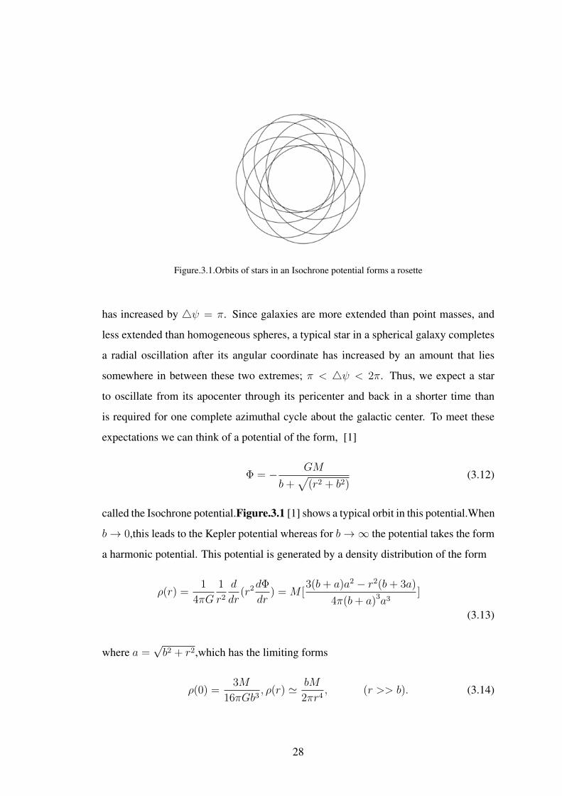
Figure.3.1.Orbits of stars in an Isochrone potential forms a rosette

has increased by 4ψ = π. Since galaxies are more extended than point masses, and

less extended than homogeneous spheres, a typical star in a spherical galaxy completes

a radial oscillation after its angular coordinate has increased by an amount that lies

somewhere in between these two extremes; π < 4ψ < 2π. Thus, we expect a star

to oscillate from its apocenter through its pericenter and back in a shorter time than

is required for one complete azimuthal cycle about the galactic center. To meet these

expectations we can think of a potential of the form, [1]

Φ = − GM

b+√

(r2 + b2)(3.12)

called the Isochrone potential.Figure.3.1 [1] shows a typical orbit in this potential.When

b→ 0,this leads to the Kepler potential whereas for b→∞ the potential takes the form

a harmonic potential. This potential is generated by a density distribution of the form

ρ(r) =1

4πG

1

r2

d

dr(r2dΦ

dr) = M [

3(b+ a)a2 − r2(b+ 3a)

4π(b+ a)3a3]

(3.13)

where a =√b2 + r2,which has the limiting forms

ρ(0) =3M

16πGb3, ρ(r) ' bM

2πr4, (r >> b). (3.14)

28

It is convenient to define an auxiliary variable s by

s ≡ −GMbΦ

= 1 +

√r2

b2+ 1,

r2

b2= s2(1− 2

s), (s ≥ 0) (3.15)

Given this one-to-one relationship between s and r, we may employ s as a radial co-

ordinate in place of r. The integrals (3.9) and (3.10) for Tr and 4ψ both involve the

infinitesimal quantity,

dI =dr√

2(E − Φ)− L2

r2

(3.16)

Eliminating r from this expression,we get

dI =b(s− 1)ds√

2Es2 − 2(2E −GM/b)s− 4GM/b− L2/b2(3.17)

As the star moves from pericenter r1 to apocenter r2, s varies from the smaller root s1

of the quadratic expression in the denominator of equation (3.17) to the larger root s2.

Thus, combining equations (3.9) and (3.17), the radial period is

Tr =2b√−2E

∫ s2

s1

(s− 1)ds√(s2 − s)(s− s1)

=2b√−2E

∫ s2

s1

ds√−s2 + (s1 + s2)s− s1s2

(−(s1 + s2)

2+ 1

)

=2b√−2E

− sin−1

−2s+ b√(s1 − s2)2

s2s1

=2πb√−2E

[1

2(s1 + s2)− 1

](3.18)

But from the denominator of equation (3.17) it follows that the roots s1 and s2 obey

s1 + s2 = 2−GM/Eb (3.19)

29

Hence the radial period is,

Tr =2πGM

(−2E)32

.

(3.20)

Note that Tr depends on the energy E but not on the angular momentum L; it is this

unique property that gives the isochrone its name.Equation (3.10), for the increment

4ψ in azimuthal angle per cycle in the radial direction, yields

M ψ = 2L

∫ s2

s1

dt

r2=

2L

b√−2E

∫ s2

s1

(s− 1)

s(s− 2)√

(s2 − s)(s− s1)ds

= π(1 +L√

L2 + 4GMb).

(3.21)

From this expression we see that π ≤ 4ψ ≤ 2π. This proves the fact that isochrone

potential neither behaves like Kepler nor like the harmonic potential,which we already

discussed. Because galaxies are more extended objects unlike point masses, a typical

star takes less time to complete one radial oscillation that what it takes to complete once

azimuthal cycle.

3.2 Rotation curves of galaxies

All stars do not rotate around the galactic centre with the same velocity. If we know

how mass is distributed, we can find the resulting gravitational force and from this we

can calculate how the positions and velocities of stars and galaxies will change over

time. As the radial distance of the star from the centre increases their velocity decreases

according to the conservation of angular momentum. This results in a differential rota-

tion of the galaxy contributing to a circular velocity given by v = Ωr. The inner parts

of the galaxy rotates faster than the outer parts.as was mentioned in the last chapter

gravity can be supported either by the centrifugal force or the random velocities of the

components of a galaxy. A galaxy forms from a huge clump of gas and dust which

30

gradually in the process of attaining the thermal equilibrium condenses to form a disk

which is the highly flattened component in which newly formed stars rotate almost in

circular orbits lying along the same plane. In this case gravity is supported against

the centrifugal force of rotation, whereas the stars in the spherically distributed halo

surrounding the disk forms in the early stages of the evolution of a galaxy where the

gravity is supported against the random velocities of motion of stars. They are called

globular clusters. Thus the ratio of Mass to Luminosity ceases to be equal to unity in the

halo as the observational data suggests.The rotation curve, a plot of rotational speed V

versus distance from the galactic center, is an indicator of the mass distribution within

the galaxy.The rotation curves of most galaxies,including our own,indicate that large

quantities of dark matter are associated with the individual galaxies. On equating the

centrifugal force and gravitational force, we get

v2c

R=

G

R2=∂Φ

∂R

It is obvious from the relation that velocity should increase linearly with the gravita-

tional potential gradient upto the extent of the disk and decrease in a Keplerian fashion

as most of the matter in the halo is dark. It could be non luminous remnants of a star

or other fragments of matter which never became luminous(Jupiter like planets, black

holes, neutrinos or monopoles) [6]. We can also use the stellar motions to tell us where

the mass is. Only luminous matter were thought to contribute to the potential. But when

the rotation curves of such galaxies were studied it was found that the circular velocity

does not decrease instead remains almost flat. The reason behind this flat curve is the

dark matter present in the interstellar medium of globular clusters of galaxies. This was

a breakthrough for those people who were searching for observational evidence of dark

matter other than gravitational lensing where gravity was found to bend the light rays

coming from distant galaxies or stars.

31

3.2.1 Orbits in axisymmetric systems

When it comes to axisymmetric systems such as disks embedded in a halo, we encounter

interesting features in the nature of orbits of the stars as was mentioned in the beginning

of the section. Thus our goal is to frame a theoretical basis to support the observational

data collected so far on different galactic rotation curves. Disk galaxies may or may not

have a bulge component at the centre. Either way the disk is believed to have a surface

density profile that decreases exponentially with the radial distance from the galactic

centre. It gives us the liberty to choose the following form of surface density to account

for the mass distribution in a disk.

Σ(R) = Σ0(−R/Rd) (3.22)

We can now determine the gravitational potential that is due to such a disk and the

properties of stellar orbits. For the ease of calculations, it is convenient to use the fact

that in axially symmetric cases, the functions [3]

Φ±(R, z) = exp(±kz)J0(kR) (3.23)

(where J0 is the Bessel function) are the solutions to the Laplace equation. Consider

now the function given by,

Φk(R, z) = exp(−k|z|)J0(kR) (3.24)

which has the discontinuity in the derivative at z = 0 given by,

limz→0+

(∂Φk

∂z

)= −kJ0(kR), lim

z→0−(−∂Φ

∂z) = +kJ0(kR) (3.25)

We know from Gauss theorem that a surface density distribution will result in a gravi-

tational potential Φk. Hence it follows that,

Σk(R) = − k

2πGJ0(kR), (3.26)

32

located at z = 0. Superposing the density distribution by using a weightage function

S(k),we find that the surface density profile,

Σ(R) =

∫ ∞0

S(k)Σk(R)dk = − 1

2πG

∫ ∞0

S(k)J0(kR)kdk, (3.27)

will generate the gravitational potential

Φ(R, z) =

∫ ∞0

S(k)Φk(R, z)dk =

∫ ∞0

S(k)J0(kR) exp(−k|z|)dk (3.28)

Though this analysis is very general and could be done with a wide class of radial

functions,Bessel functions make it a lot easier due to the fact that it is invertible [3].i.e.

S(k) = −2πG

∫ ∞0

J0(kR)Σ(R)RdR (3.29)

Using this in eqn(3.28),we can express the potential directly in terms of the density

Σ(R), thereby providing the complete solution to the problem. Given the form of the

potential, we can also determine the rotation velocity in terms of S(k);

v2c (R) = R(

∂Φ

∂R)z=0

= −R∫ ∞

0

S(k)J1(k)kdk (3.30)

Similarly we can obtain surface density in terms of rotation curves in the following

manner;we know that for axisymmetric disks,z=0.Hence the surface density becomes,

Σ(R) = − 1

2πG

∫ ∞0

S0(k)J0(kR)kdk

(3.31)

and the potential is expressed in terms of Bessel functions as,

Φ(R, 0) =

∫ ∞0

dkS0(k)J0(kR)

∂Φ(R, 0)

∂R=

∂

∂R

∫ ∞0

dkS0(k)J0(kR)

(3.32)

33

Using the property of Bessel functions,

dJ0(x)

dx= −J1(x)

we obtain the rotation velocity as,

v2c = −R

∫ ∞0

dkkS0(k)J1(kR) = 2πGR

∫ ∞0

dkkJ1(kR)

∫ ∞0

J0(kR′)Σ(R′)R′dR

(3.33)

Applying to eqn(3.33), the inversion formula for Hankel transform,we get

S0(k) = −∫ ∞

0

dR′v2c (R

′)J1(kR′) (3.34)

Substituting the above equation in eqn(3.31)

Σ(R) =1

2πG

∫ ∞0

J0(kR)kdk

∫ ∞0

dR′v2c (R

′)J1(kR′)

(3.35)

For an exponential disk, we can evaluate the integral in eq. to obtain S(k),

S(k) = −2πGΣ0

∫ ∞0

J0(kR) exp(−RRd

)RdR (3.36)

On substituting kR = x,

S(k) = −2πGΣ0

k2

∫ ∞0

J0(x) exp(− x

kRd

)xdx (3.37)

We know from the properties of Bessel functions [9] for a = ±1,∫x exp(ax)J0(x)dx

= exp(ax)

[ax

a2 + 1J0(x) +

x

a2 + 1J1(x)

]− a

a2 + 1

∫exp(−ax)J(x)dx (3.38)

34

Using the above property, equation(3.37) becomes

S(k) = −2πGΣ0

k2

[− a

a2 + 1

∫ ∞0

exp(ax)J0(x)dx

](3.39)

where a = −1/kRd.We also know that,

∫ ∞0

exp(ax)J0(x)dx =1√

a2 + b2(3.40)

Substituting the value of ’a’ back into eqn(3.39) and using the above property,we get

S(k) = − 2πGΣ0R2d

[1 + (kRd)2]

32

(3.41)

The potential is now given by,

Φ(R, z) = −2πGΣ0R2d

∫ ∞0

J0(kR) exp(−k|z|)

[1 + (kRd)2]

32

dk (3.42)

which unfortunately cannot be expressed in simple closed form for arbitrary z.In the

z = 0 plane,however, the result can be expressed in terms of modified Bessel functions

by

Φ(R, 0) = −πGΣ0R[I0(y)K1(y)− I1(y)K0(y)], y ≡ R

2Rd

(3.43)

with the corresponding circular speed

v2c (R) = R

(∂Φ

∂R

)= 4πGΣ0Rdy

2[I0(y)K0(y)− I1(y)K1(y)]. (3.44)

Figure 3.2. shows v2c (R)/4πGΣ0Rd as a function of (R/Rd). It is evident from the

figure that the rotation curves have to do with the luminous matter distribution in the

plane of a disk. As is expected from the constant M/L ratio for a disk where the only

components contributing to the gravitational potential are the stars, gas and the inter-

stellar dust, the rotational velocity reaches a peak almost at a distance twice as large the

35

Figure.3.2.Rotation curve of disk

disk radius Rd and falls off as V (r) ∝ r−1/2 in the outer parts. But the curves obtained

theoretically by assuming an exponentially varying surface density profile failed to be

consistent with the observed rotation curves as it was found that the rotation curve flat-

tens out or falls only slowly with the radius beyond a certain distance from the galactic

centre. This led us to think of another component which can effectively account for this

major discrepancy in the nature of the curves.

3.2.2 Evidence for the existence of dark matter

Neptune was discovered in the year of 1846, when it struck the intelligent minds on

Earth that there was something unusual about the kinematics of Uranus. Such anomalies

that we see often reveals the hidden. The dark matter is mostly hidden in the darkness

of the universe that even a slight evidence of its existence can be a guide to understand-

ing our universe better. As far as the search for this most dominant component in the

galaxies are concerned, the rotation curves act as the primary tool to locate and study

their distribution. The spectroscopic studies based on the Doppler shifts in the emitted

or absorbed lines can tell us a great deal about the rotation curves of galaxies. Of all

36

Figure.3.3.Rotation curve of a disk embedded in a halo

frequencies in the EM spectrum, the radio frequencies are best suited to probe rotation

curves as the most decisive observations come from the studies of cold atomic hydro-

gen which do not confine just to the disk alone. The density profile of the spherically

distributed halo needs to be obtained by a comparison of the observed rotation curve

with the one that is due to the exponential disk. When this comparison was made, the

density profile of the dark halo,responsible for the flat rotation curves, resembled that

of an isothermal sphere which was already discussed in section 2.3 of the last chapter.

Thus a density function given below would be appropriate to account for a spherically

symmetric dark halo. [3]

ρh(r) =ρh(0)

1 + (r/a)γ(3.45)

where a is the radius of the halo which being uncertain usually varies from 7kpc to

12kpc. γ can take values in the range 1.9 < γ < 2.9. This halo produces a rotational

velocity given by,

v2h(r) =

GMh(rh)

r=

4πG

r

∫ r

0

dxx2ρh(x) (3.46)

37

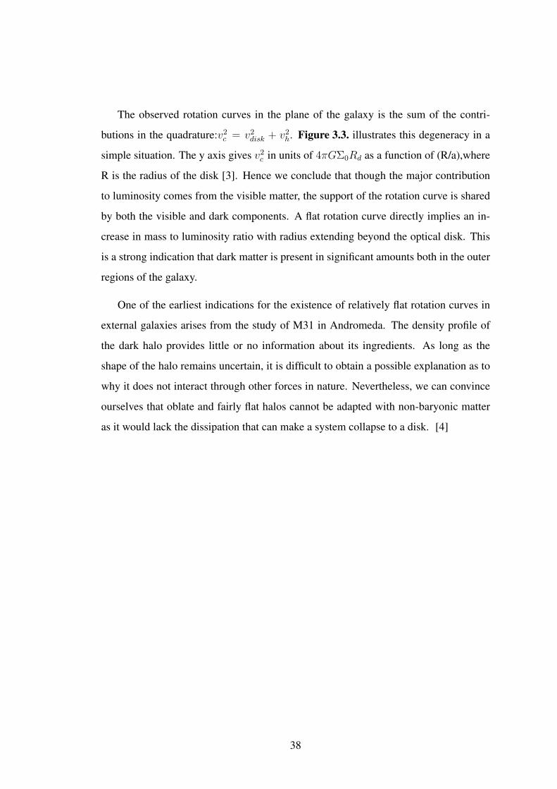
The observed rotation curves in the plane of the galaxy is the sum of the contri-

butions in the quadrature:v2c = v2

disk + v2h. Figure 3.3. illustrates this degeneracy in a

simple situation. The y axis gives v2c in units of 4πGΣ0Rd as a function of (R/a),where

R is the radius of the disk [3]. Hence we conclude that though the major contribution

to luminosity comes from the visible matter, the support of the rotation curve is shared

by both the visible and dark components. A flat rotation curve directly implies an in-

crease in mass to luminosity ratio with radius extending beyond the optical disk. This

is a strong indication that dark matter is present in significant amounts both in the outer

regions of the galaxy.

One of the earliest indications for the existence of relatively flat rotation curves in

external galaxies arises from the study of M31 in Andromeda. The density profile of

the dark halo provides little or no information about its ingredients. As long as the

shape of the halo remains uncertain, it is difficult to obtain a possible explanation as to

why it does not interact through other forces in nature. Nevertheless, we can convince

ourselves that oblate and fairly flat halos cannot be adapted with non-baryonic matter

as it would lack the dissipation that can make a system collapse to a disk. [4]

38

CHAPTER 4

Conclusion

In this report, starting with the description of galaxies, assuming them to have attained

their equilibrium configuration through years of evolution, we assigned a distribution

function constant in time to them in order to study the different structures they evolve

into. We saw in chapter 2 that, the dynamics of a galaxy can be explained with the help

of the collisionless Boltzmann equation which immediately follows from the fact that

stars in a galaxy are not discrete infinite dips in the potential but are rather distributed

smoothly in space. With this idea in mind, we could obtain the gravitational potentials

of some isotropic and anisotropic models of galaxies classified based on the form of

their distribution function.

In chapter 3, we found that apart from the stars, there were other components that

tend to influence the velocity with which they rotate about the galactic centre. This

realization followed from the flat rotation curves that were inferred from the spectro-

scopic studies of the motion of stars, gas and dust in a galaxy. We obtained the same

flat rotation curves of galaxies theoretically assigning a density function similar to that

of an isothermal sphere discussed in chapter 2 simply to account for the spherical sym-

metry of the dark halo surrounding the highly luminous disks of the galaxies. Thus

it was found that the theoretical prediction of rotation curves taking a Keplerian form

(i.e.∝ r−1/2) in the outer parts was wrong as the dark matter residing in the halo pro-

vides a fairly good amount of potential to maintain a flat rotation curve even when there

is little or no luminous matter. Despite the fact that we are nothing but a frivolous dust

in this universe, there lies so much beyond our naked eyes expecting to be revealed

sometime in the near future through our constant efforts to understand the universe bet-

ter. Dark matter is what tops the list. Though we were able to study how dark matter is

distributed it is still a matter of dedicated research as to what makes up dark matter.

REFERENCES

[1] James Binney, Scott Tremaine. Galactic dynamics, Second edition, Princeton Series

in Astrophysics, Princeton University Press, 1987

[2] T.Padmanabhan, Theoretical Astrophysics.Vol.I:Astrophysical Processes, Cam-

bridge University Press, Cambridge,2000.

[3] T.Padmanabhan, Theoretical Astrophysics.Vol.III:Galaxies and Cosmology, Cam-

bridge University Press, Cambridge,2000.

[4] Bertin, G. (Giuseppe), Dynamics of galaxies, Second edition, Cambridge Univer-

sity Press, Cambridge, 2000.

[5] Hale Bradt. Astrophysics Processes. Cambridge University Press, Cambridge,

2008.

[6] Rubin, Vera(1997). Bright galaxies, dark matter. Woodbury, NY: AIP Press.

[7] Peter Schneider. Extragalactic Astronomy, Springer-Verlag, Berlin, Heidelberg

2006.

[8] Houjun Mo, Frank van den Bosch, Simon White. Galaxy evolution and formation,

Cambridge University Press, Cambridge, 2010.

[9] Spiegel,.Schaum’s. Mathematical Handbook of Formulas and

Tables.(0070382034)(McGraw-Hill,.1998).

[10] Linda S. Sparke, Gallagher. Galaxies in the Universe, Cambridge University Press,

Cambridge, 2007.

[11] T.S. van Albada, J.N. Bahcall, K. Begeman und R. Sancisi: Astro-

phys.J.,295(1985)305

40