rotation and neoclassical ripple transport in iter€¦ · rotation and neoclassical ripple...
TRANSCRIPT
Rotation and Neoclassical Ripple Transport in ITER
Elizabeth J. Paul1 Matt Landreman1 Francesca Poli2
Don Spong3 Hakan Smith4 William Dorland1
1University of Maryland
2Princeton Plasma Physics Laboratory
3Oak Ridge National Laboratory
4Max-Planck-Institut fur Plasmaphysik
July 17, 2017
Elizabeth Paul (University of Maryland) Rotation and Neoclassical Transport in ITER July 17, 2017 1 / 37

Motivation
Sufficient toroidal rotation is critical to ITER’s success
Magnitude of rotation can stabilize resistive wall modes (RWMs)Rotation shear can decrease microinstabilities and promote formationof ITBs
Sources and sinks of rotation in ITER
Neutral beams: sourceTurbulent intrinsic rotation: sourceNeoclassical toroidal viscosity (NTV): typically sink
I will focus on computing NTV torque caused by symmetry-breakingin ITER
Elizabeth Paul (University of Maryland) Rotation and Neoclassical Transport in ITER July 17, 2017 2 / 37
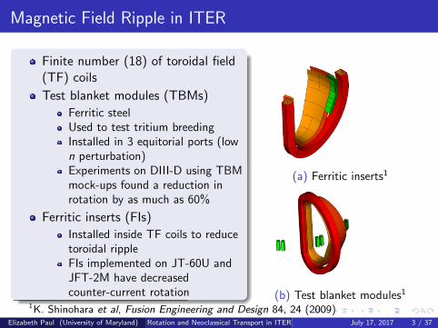
Magnetic Field Ripple in ITER
Finite number (18) of toroidal field(TF) coils
Test blanket modules (TBMs)
Ferritic steelUsed to test tritium breedingInstalled in 3 equitorial ports (lown perturbation)Experiments on DIII-D using TBMmock-ups found a reduction inrotation by as much as 60%
Ferritic inserts (FIs)
Installed inside TF coils to reducetoroidal rippleFIs implemented on JT-60U andJFT-2M have decreasedcounter-current rotation
(a) Ferritic inserts1
(b) Test blanket modules1
1K. Shinohara et al, Fusion Engineering and Design 84, 24 (2009)Elizabeth Paul (University of Maryland) Rotation and Neoclassical Transport in ITER July 17, 2017 3 / 37

Neoclassical Toroidal Viscosity (NTV)
When toroidal symmetry is broken, trapped particles may wander offa flux surface
Banana diffusion: particles trapped poloidally (bananas) can driftradially, as J|| becomes a function of toroidal angleRipple trapping: if local ripple wells exist along a field line and thecollisionality is sufficiently small, particles can become helically trapped
ITER’s collisionality may be sufficiently low such that this effect isimportant
For a general electric field, the ion and electron fluxes are not identicalRadial current induces a J × B torque, which is typicallycounter-current
τNTV = −Bθ√g∑a
ZaeΓψ,a
Elizabeth Paul (University of Maryland) Rotation and Neoclassical Transport in ITER July 17, 2017 4 / 37

Classes of Trapped Particles
The n = 18 ripple may allow for local trapping in addition to bananadiffusion
We must compute NTV torque such that all particle trajectories areaccounted for
B along field line at r/a = 0.9 due to TF ripple
Elizabeth Paul (University of Maryland) Rotation and Neoclassical Transport in ITER July 17, 2017 5 / 37
Method of Computing NTV
Model of steady-state scenario profiles using TRANSP2
Includes NBI model (NUBEAM), EPED1 pedestal model, and currentdiffusive ballooning mode transport model
Calculate 3D MHD equilibrium using free boundary VMECVacuum FI and TBM magnetic fields (computed with FEMAG1)Filamentary coil modelsPressure and q profiles (from TRANSP)
Estimate rotation (Er ) to find torqueSemi-analytic intrinsic rotation modelNBI torque (from NUBEAM)Use SFINCS to determine Er consistent with rotation
Solve drift kinetic equation to compute radial particle flux usingSFINCS
Using profiles, geometry, and Er as explained aboveMakes no assumptions about magnitude of perturbing field andaccounts for all collisionality regimes
2F. Poli et al, Nuclear Fusion 54, 7 (2014)1K. Shinohara et al, Fusion Engineering and Design 84, 24 (2009)
Elizabeth Paul (University of Maryland) Rotation and Neoclassical Transport in ITER July 17, 2017 6 / 37

Roadmap for Remainder of Talk
ITER steady state scenario
VMEC equilibrium with ripple
Rotation model (without NTV) to estimate Er
SFINCS calculations of particle and heat fluxes
Comparison of NTV torque with analytic scaling predictions and othertoroidal torques
Tangential magnetic drift models
Elizabeth Paul (University of Maryland) Rotation and Neoclassical Transport in ITER July 17, 2017 7 / 37

ITER Steady State Scenario2
Scenario Parameters
33 MW NBI, 20 MW EC, 20MW LH heating
9 MA toroidal plasmacurrent
Fusion gain Q = 5
Simulated using TokamakSimulation Code (TSC) inIPS framework andTRANSP
NBI source modeled usingNUBEAM
2F. Poli et al, Nuclear Fusion 54, 7 (2014)Elizabeth Paul (University of Maryland) Rotation and Neoclassical Transport in ITER July 17, 2017 8 / 37

Free Boundary VMEC Equilibrium
δB =Bmax − Bmin
Bmax + Bmin
TBMs increase magnitudeof ripple near outboardmidplane
FIs decrease poloidal extentof ripple
Ripple magnitude decreaseswith radius
Elizabeth Paul (University of Maryland) Rotation and Neoclassical Transport in ITER July 17, 2017 9 / 37

Free Boundary VMEC Equilibrium
Ferritic inserts decreasemagnitude of rippleaway from midplane
TBMs locally decreasemagnetic flux nearmidplane
Elizabeth Paul (University of Maryland) Rotation and Neoclassical Transport in ITER July 17, 2017 10 / 37
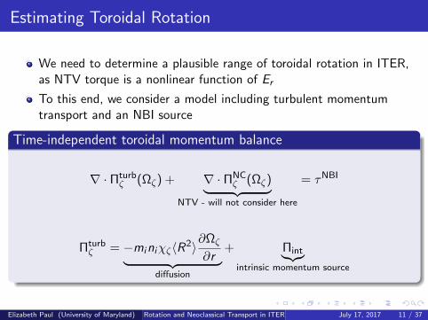
Estimating Toroidal Rotation
We need to determine a plausible range of toroidal rotation in ITER,as NTV torque is a nonlinear function of Er
To this end, we consider a model including turbulent momentumtransport and an NBI source
Time-independent toroidal momentum balance
∇ · Πturbζ (Ωζ) + ∇ · ΠNC
ζ (Ωζ)︸ ︷︷ ︸NTV - will not consider here
= τNBI
Πturbζ = −miniχζ〈R2〉
∂Ωζ
∂r︸ ︷︷ ︸diffusion
+ Πint︸︷︷︸intrinsic momentum source
Elizabeth Paul (University of Maryland) Rotation and Neoclassical Transport in ITER July 17, 2017 11 / 37
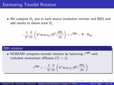
Estimating Toroidal Rotation
We compute Ωζ due to each source (turbulent intrinsic and NBI) andadd results to obtain total Ωζ
− 1
V ′∂
∂r
(V ′miniχζ〈R2〉
∂Ωζ
∂r
)= τNBI −∇ · Πint
NBI rotation
NUBEAM computes toroidal rotation by balancing τNBI withturbulent momentum diffusion (Pr = 1)
τNBI = − 1
V ′∂
∂r
(V ′miniχi 〈R2〉
∂Ωζ
∂r
)
Elizabeth Paul (University of Maryland) Rotation and Neoclassical Transport in ITER July 17, 2017 12 / 37
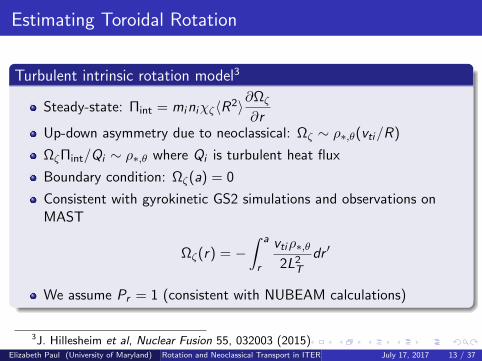
Estimating Toroidal Rotation
Turbulent intrinsic rotation model3
Steady-state: Πint = miniχζ〈R2〉∂Ωζ
∂rUp-down asymmetry due to neoclassical: Ωζ ∼ ρ∗,θ(vti/R)
ΩζΠint/Qi ∼ ρ∗,θ where Qi is turbulent heat flux
Boundary condition: Ωζ(a) = 0
Consistent with gyrokinetic GS2 simulations and observations onMAST
Ωζ(r) = −∫ a
r
vtiρ∗,θ2L2
T
dr ′
We assume Pr = 1 (consistent with NUBEAM calculations)
3J. Hillesheim et al, Nuclear Fusion 55, 032003 (2015)Elizabeth Paul (University of Maryland) Rotation and Neoclassical Transport in ITER July 17, 2017 13 / 37

Estimating Toroidal Rotation – Results
Parra4 scaling:Vζ ∼ Ti/IP ∼ 100 km/s
Rice5 scaling:Vζ ∼Wp/Ip ∼ 400 km/s
A critical Alfven Machnumber,MA = Ωζ(0)/ωA & 5%,must be achieved forstabilization of theRWM6
4F. Parra et al, Physical Review Letters 108, 095001 (2012)5J. Rice et al, Nuclear Fusion 47, 1618 (2007)6Liu et al, Nuclear Fusion 44, 232 (2004)
Elizabeth Paul (University of Maryland) Rotation and Neoclassical Transport in ITER July 17, 2017 14 / 37

SFINCS Calculations
Drift kinetic equation solved for fa1 on a flux surface
(v||b + vE + vma) · (∇fa1)W ,µ − C (fa1) =
−vma · ∇ψ(∂fa0
∂ψ
)W ,µ
+Zaev||B〈E||B〉
Ta〈B2〉fa0
Tangential magnetic drifts will not be included for most of thefollowing calculations (stay tuned)
Inductive electric field is small for this steady-state scenario (loopvoltage ∼ 10−4V ), so this term is not retained
C – linearized Fokker-Planck operator
3 species (e, D, T )
Elizabeth Paul (University of Maryland) Rotation and Neoclassical Transport in ITER July 17, 2017 15 / 37

NTV Torque Density
r/a = 0.9
Circle indicates neoclassical offset rotation (≈ −10 km/s)
Increased∣∣τNTV
∣∣ due to 1/ν transport near Er = 0
Addition of FIs decreases∣∣τNTV
∣∣ by ∼ 75%
Elizabeth Paul (University of Maryland) Rotation and Neoclassical Transport in ITER July 17, 2017 16 / 37
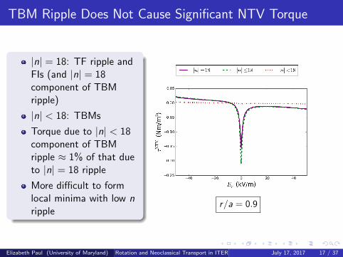
TBM Ripple Does Not Cause Significant NTV Torque
|n| = 18: TF ripple andFIs (and |n| = 18component of TBMripple)
|n| < 18: TBMs
Torque due to |n| < 18component of TBMripple ≈ 1% of that dueto |n| = 18 ripple
More difficult to formlocal minima with low nripple
r/a = 0.9
Elizabeth Paul (University of Maryland) Rotation and Neoclassical Transport in ITER July 17, 2017 17 / 37

NTV Torque - Radial Dependence
At large Er , τNTV does not depend strongly on radius
At small |Er |,∣∣τNTV
∣∣ increases with decreasing radius due to
T7/2i scaling in the 1/ν regime
Elizabeth Paul (University of Maryland) Rotation and Neoclassical Transport in ITER July 17, 2017 18 / 37
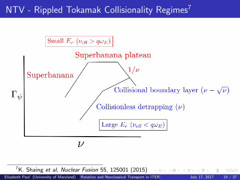
NTV - Rippled Tokamak Collisionality Regimes7
7K. Shaing et al, Nuclear Fusion 55, 125001 (2015)Elizabeth Paul (University of Maryland) Rotation and Neoclassical Transport in ITER July 17, 2017 19 / 37
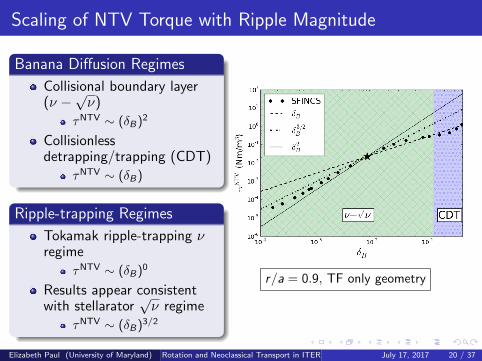
Scaling of NTV Torque with Ripple Magnitude
Banana Diffusion Regimes
Collisional boundary layer(ν −
√ν)
τNTV ∼ (δB)2
Collisionlessdetrapping/trapping (CDT)
τNTV ∼ (δB)
Ripple-trapping Regimes
Tokamak ripple-trapping νregime
τNTV ∼ (δB)0
Results appear consistentwith stellarator
√ν regime
τNTV ∼ (δB)3/2
r/a = 0.9, TF only geometry
Elizabeth Paul (University of Maryland) Rotation and Neoclassical Transport in ITER July 17, 2017 20 / 37

Neoclassical Heat Flux
r/a = 0.9
Toroidalsymmetry-breakingcauses additionalradial heat flux overaxisymmetric level
Insignificant incomparison toturbulent heat fluxQi ≈ 0.2 MW/m2
(estimated fromvolume integral ofheating and fusionpower)
Elizabeth Paul (University of Maryland) Rotation and Neoclassical Transport in ITER July 17, 2017 21 / 37

Tangential Magnetic Drifts
For calculations presented previously, vm · ∇f1 was not included in thedrift kinetic equation solved by SFINCS
SFINCS does not include radial coupling of f1, so ∇ψ component ofvm is not retained when this term is included in the kinetic equation,which introduces a coordinate dependence
Elizabeth Paul (University of Maryland) Rotation and Neoclassical Transport in ITER July 17, 2017 22 / 37

Tangential Magnetic Drifts
We compare two tangential drift models
Typical definition of ∇B and curvature drifts
Coordinate-dependent form and does not conserve phase space whenradially local assumption is made
vm =v2⊥ + 2v2
||
2ΩB2B ×∇B +
v2||
ΩB∇× B
For v⊥m , the ∇B drift has been projected onto a flux surface
This eliminates dependence on choice of toroidal and poloidal anglesThis form has been shown8 to eliminate the need for additional particleand heat sources due to the radially local assumptionRegularization required for conservation performed by droppingcurvature drift (deeply-trapped assumption)
v⊥m =v2⊥
2ΩB2(B ×∇ψ)
∇ψ · ∇B|∇ψ|2
8H. Sugama et al, Physics of Plasmas 23, 042502 (2016)Elizabeth Paul (University of Maryland) Rotation and Neoclassical Transport in ITER July 17, 2017 23 / 37

Comparison of Tangential Magnetic Drift Models
r/a = 0.7, TF only geometry
At this radius, ρ∗ ∼ ν∗Inclusion of vm · ∇f1 shifts resonant peak to Er such that(vm + vE ) ≈ 0 (superbanana plateau resonance)
Differences between tangential drift models are appreciable only forsmall |Er |
Elizabeth Paul (University of Maryland) Rotation and Neoclassical Transport in ITER July 17, 2017 24 / 37
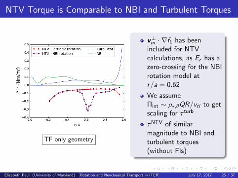
NTV Torque is Comparable to NBI and Turbulent Torques
TF only geometry
v⊥m · ∇f1 has beenincluded for NTVcalculations, as Er has azero-crossing for the NBIrotation model atr/a = 0.62
We assumeΠint ∼ ρ∗,θQR/vti to getscaling for τ turb
τNTV of similarmagnitude to NBI andturbulent torques(without FIs)
Elizabeth Paul (University of Maryland) Rotation and Neoclassical Transport in ITER July 17, 2017 25 / 37

Conclusions
SFINCS can be applied to compute neoclassical ripple transportwithout the need for simplifying assumptions about transport regimes,the magnitude of ripple, or the collision operator
The TBM (low n) ripple will not cause significant NTV torque inITER
The TF ripple (without FIs) would cause NTV torque which is similarin magnitude to both the turbulent intrinsic and NBI torques and willsignificantly damp rotation
The inclusion of FIs will decrease the magnitude of NTV torque by≈ 75%
Tangential drift models must be considered when Er is near azero-crossing
Scaling of NTV torque with ripple magnitude indicates localripple-trapping may be significant for ITER
Elizabeth Paul (University of Maryland) Rotation and Neoclassical Transport in ITER July 17, 2017 26 / 37

Application of Adjoint Methods to Stellarator CoilOptimization (Work in Progress)
Elizabeth J. Paul1 Matt Landreman1 William Dorland1
1University of Maryland
July 17, 2017
Elizabeth J. Paul (University of Maryland) Adjoints & Stellarator Coil Optimization July 17, 2017 27 / 37
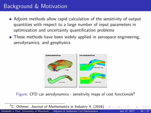
Background & Motivation
Adjoint methods allow rapid calculation of the sensitivity of outputquantities with respect to a large number of input parameters inoptimization and uncertainty quantification problems
These methods have been widely applied in aerospace engineering,aerodynamics, and geophysics
Figure: CFD car aerodynamics - sensitivity maps of cost functionals9
9C. Othmer, Journal of Mathematics in Industry 4, (2016)Elizabeth J. Paul (University of Maryland) Adjoints & Stellarator Coil Optimization July 17, 2017 28 / 37

Statement of Constrained Optimization Problem
minpχ2(u,p) subject to F (u,p) = 0
Cost functional: χ2(u,p)
Input parameters: pState variables: u(p)
State equation: F (u,p) = 0
For linear system: A(p)u(p)− b(p) = 0
Elizabeth J. Paul (University of Maryland) Adjoints & Stellarator Coil Optimization July 17, 2017 29 / 37

Sensitivity for Linear Constrained OptimizationThe Hard Way
∂χ2
∂pi
∣∣∣∣F=0
=∂χ2
∂pi+∂χ2
∂u
(∂u∂pi
)F=0
∂χ2
∂piand
∂χ2
∂ucan be analytically differentiated (easy to compute)
Computing
(∂u∂pi
)F=0
requires np = length(p) solves of linear system
Can be obtained by finite differencing in piOr by inverting A np times(
∂u∂pi
)F=0
= −A−1
(∂A∂pi
u − ∂b∂pi
)(1)
Elizabeth J. Paul (University of Maryland) Adjoints & Stellarator Coil Optimization July 17, 2017 30 / 37

Sensitivity for Linear Constrained OptimizationThe Adjoint Way
(∂u∂pi
)F=0
= −A−1
(∂A∂pi
u − ∂b∂pi
)∂χ2
∂pi
∣∣∣∣F=0
=∂χ2
∂pi− ∂χ2
∂uA−1︸ ︷︷ ︸
qT
(∂A
∂piu − ∂b
∂pi
)
Solve adjoint equation once: ATq =
(∂χ2
∂u
)T
Compute∂χ2
∂pi
∣∣∣∣F=0
for all pi with just two linear solves (forward and
adjoint)
Form inner product with q to compute sensitivity for each pi
Elizabeth J. Paul (University of Maryland) Adjoints & Stellarator Coil Optimization July 17, 2017 31 / 37

Stellarator Coil Optimization with REGCOIL10
REGCOIL computes stellarator coil shapes given a target plasmashape and coil winding surface
Current density K = n ×∇Φ
Current potential Φ(θ, ζ) =
determined by REGCOIL︷ ︸︸ ︷ΦSV(θ, ζ) +
determined by plasma current︷ ︸︸ ︷Gζ
2π+
Iθ
2π
Figure: Coil and plasma surfaces for W7-X
10Landreman, Nuclear Fusion 57, 046003 (2017)Elizabeth J. Paul (University of Maryland) Adjoints & Stellarator Coil Optimization July 17, 2017 32 / 37
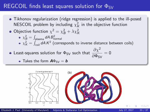
REGCOIL finds least squares solution for ΦSV
Tikhonov regularization (ridge regression) is applied to the ill-posedNESCOIL problem by including χ2
K in the objective function
Objective function χ2 = χ2B + λχ2
K
χ2B =
∫plasma
dAB2normal
χ2K =
∫coil
dAK 2 (corresponds to inverse distance between coils)
Least-squares solution for ΦSV such that∂χ2
∂ΦSV= 0
Takes the form AΦSV = b
Current potential contours and coil shapes computed for NCSX geometryElizabeth J. Paul (University of Maryland) Adjoints & Stellarator Coil Optimization July 17, 2017 33 / 37
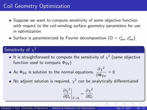
Coil Geometry Optimization
Suppose we want to compute sensitivity of some objective functionwith respect to the coil-winding surface geometry parameters for usein optimization
Surface is parameterized by Fourier decomposition (Ω = r cmn, zsmn)
Sensitivity of χ2
It is straightforward to compute the sensitivity of χ2 (same objectivefunction used to compute ΦSV)
As ΦSV is solution to the normal equations,∂χ2
∂ΦSV= 0
No adjoint solution is required, χ2 can be analytically differentiated
∂χ2
∂Ωi
∣∣∣∣F=0
=∂χ2
∂Ωi
Elizabeth J. Paul (University of Maryland) Adjoints & Stellarator Coil Optimization July 17, 2017 34 / 37

Adjoints Are Needed to Compute Sensitivity of OtherObjective Functions
If we would like to find the sensitivity with respect of a differentobjective function, χ2, than that used to solve for ΦSV, we must finda solution to the adjoint equation
ATq =
(∂χ2
∂ΦSV
)T
AT must be inverted with a different RHS for each objective functionof interest
For example, we may want to compute sensitivity of χ2B or χ2
K withrespect to Ω
Elizabeth J. Paul (University of Maryland) Adjoints & Stellarator Coil Optimization July 17, 2017 35 / 37
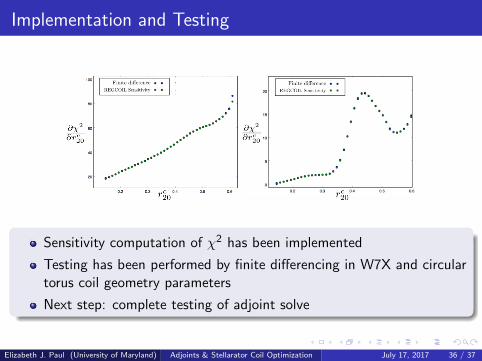
Implementation and Testing
Sensitivity computation of χ2 has been implemented
Testing has been performed by finite differencing in W7X and circulartorus coil geometry parameters
Next step: complete testing of adjoint solve
Elizabeth J. Paul (University of Maryland) Adjoints & Stellarator Coil Optimization July 17, 2017 36 / 37
Conclusions
Adjoint methods allow for fast computation of gradients with respectto input parameters
This can be applied to the optimization of a coil winding surface inREGCOIL, requiring only 2 linear solves to compute gradients withrespect to all geometry parameters (for W7X, length(Ω) ≈ 50)
Currently being implemented and tested (stay tuned for results)
Eventually this extended REGCOIL method could be implementedwithin an optimization loop
Elizabeth J. Paul (University of Maryland) Adjoints & Stellarator Coil Optimization July 17, 2017 37 / 37