arX

iv:1

002.

1206

v1 [

phys

ics.

clas

s-ph

] 5

Feb

201

0

ROTATING ELECTROMAGNETIC WAVES

IN TOROID-SHAPED REGIONS

CLAUDIA CHINOSIDipartimento di Scienze e Tecnologie Avanzate

Universita del Piemonte OrientaleViale Teresa Michel 11, 15121 Alessandria, Italy

chinosi@unipmn.it

LUCIA DELLA CROCEDipartimento di Matematica

Universita di PaviaVia Ferrata 1, 27100 Pavia, Italy

lucia.dellacroce@unipv.it

DANIELE FUNARODipartimento di Matematica

Universita di Modena e Reggio EmiliaVia Campi 213/B, 41125 Modena, Italy

daniele.funaro@unimore.it

Abstract

Electromagnetic waves, solving the full set of Maxwell equationsin vacuum, are numerically computed. These waves occupy a fixedbounded region of the three dimensional space, topologically equiva-lent to a toroid. Thus, their fluid dynamics analogs are vortex rings.An analysis of the shape of the sections of the rings, depending onthe angular speed of rotation and the major diameter, is carried out.Successively, spherical electromagnetic vortex rings of Hill’s type aretaken into consideration. For some interesting peculiar configurations,explicit numerical solutions are exhibited.

Keywords: Electromagnetism; Solitary wave; Optimal set; Toroid; Hill’svortex.

PACS Nos.: 41.20.Jb; 47.32.Ef; 02.70.Dh

Published in the International Journal of Modern Physics C, Vol. 21, No. 1(2010), pp. 11-32. DOI: 10.1142/S0129183110014926

1

1 Introduction

We start by recalling that the classical set of Maxwell equations in vacuumhas the form:

∂E

∂t= c2curlB (1)

divE = 0 (2)

∂B

∂t= − curlE (3)

divB = 0 (4)

where c is the speed of light and the two fields E and cB have the samedimensions.

It is customary to introduce the potentials A and Φ such that:

B =1

ccurlA E = − 1

c

∂A

∂t− ∇Φ (5)

By this assumption, equations (3) and (4) are automatically satisfied. Inaddition, we require that the vector and the scalar potentials are related bythe following Lorenz gauge condition:

divA +1

c

∂Φ

∂t= 0 (6)

Furthermore, one can deduce the two wave equations:

∂2A

∂t2− c2∆A = 0 (7)

∂2Φ

∂t2− c2∆Φ = 0 (8)

We are concerned with studying, from the numerical viewpoint, the de-velopment of a solitary electromagnetic wave, trapped in a bounded regionof space having a toroid shape. In the cylindrical case (equivalent to a 2-D problem), and partly for 3-D problems, this analysis was proposed andcarried out in Ref. [1]. There, the goal was to simulate stable elementarysubatomic particles by means of rotating photons. Here, we would like tocontinue the discussion of the 3-D case, because the subject might be ofmore general interest. Since exact solutions are only available in special sit-uations, we shall make use of finite element techniques to approximate the

2

model equations. In order to determine solutions of the vector wave equa-tion, confined in appropriate steady domains, we will perform an in-depthanalysis of the lower spectrum of a suitable elliptic operator, in dependanceof the shape and magnitude of the regions. In particular, we will be con-cerned with those domains realizing the coincidence of the fourth and thefifth eigenvalues of the differential operator. The reasons for this choice willbecome clear to the reader as we proceed with the investigation.

The structures we consider in this paper display a strong analogy withfluid dynamics vortex rings (see for instance Ref. [2], [3], [4]). For this reason,the techniques we apply here may be useful to get additional results in thestudy of the development of fluid vortices. As a matter of fact, peculiarconfigurations are going to be presented and discussed, opening the path toan interesting scenario for future extensions.

2 The Cylindrical Case

Let us quickly review the results obtained in Ref. [1], concerning wavesrotating around the axis of a cylinder. The magnetic field is oriented in thesame direction as the z-axis, so that the electric field lays on the orthogonalplane. The variables are expressed in cylindrical coordinates (r, z, φ). Thesolutions, however, will not depend on z.

Several options are examined in Ref. [1], here we show the most signifi-cant one, that will be used later to construct the toroid case. We denote byω a positive parameter which characterizes the frequency of rotation of thewave: ν = cω/π. Up to multiplicative constant, the two vector fields aregiven by:

E =

(

2J2(ωr)

ωrcos(cωt− 2φ), 0, J ′

2(ωr) sin(cωt− 2φ)

)

B =1

c

(

0, J2(ωr) cos(cωt− 2φ), 0)

(9)

for 0 ≤ φ < 2π, 0 ≤ r ≤ δ0/ω and any z. The fields in (9) are defined on adisk of radius δ0/ω, whose size is inversely proportional to the angular speedof rotation. In Ref. [1] , figure 5.7, the reader can see the displacement ofthe electric field for t = 0 (some on-line animations can be viewed in Ref. [5],rotating photons).

In (9) we find the Bessel function Jk (see, e.g., Ref. [6]) that solves the

3

following differential equation:

J ′′

k (x) +J ′

k(x)

x− k2Jk(x)

x2+ Jk(x) = 0 (10)

It is also useful to recall that Bessel functions are connected by the relations:

J ′

k(x) +kJk(x)

x= Jk−1(x) (11)

Jk+1(x) =2kJk(x)

x− Jk−1(x) (12)

The quantity δ0 ≈ 5.135622 turns out to be the first zero of J2. In thisway, for r = δ0/ω, the components E1 and B2 are zero. Note also that E

and B vanish for r = 0, since Jk(x) decays as xk for x → 0. The choicek = 1 is not permitted because it does not allow to prolong with continuitythe fields up to r = 0, although, one could take into consideration solutionsfor k integer greater than 2:

E =

(

kJk(ωr)

ωrcos(cωt− kφ), 0, J ′

k(ωr) sin(cωt− kφ)

)

B =1

c

(

0, Jk(ωr) cos(cωt− kφ), 0)

(13)

The idea is to simulate a k-body rotating system in equilibrium. This some-how explains why the case k = 1 is not going to produce meaningful solu-tions.

For k = 2, the electromagnetic fields in (9) are generated by the followingpotentials:

A = − 1

ω

(

J3(ωr) sin(cωt− 2φ), 0 , J3(ωr) cos(cωt− 2φ))

Φ = − 1

ωJ2(ωr) cos(cωt− 2φ)

satisfying the Lorenz condition (6) and the equations (7)-(8). The readercan check this by direct differentiation. We observe that A1 and A3 have aphase difference of 45 degrees, since: sin(cωt−2φ) = cos(cωt−2(φ+π/4)).Denoting by a(r) = J3(ωr) the term depending only on the radial variable,we easily discover that (see (10) for k = 3):

−(

d2

dr2+

1

r

d

dr− 9

r2

)

a = ω2a (14)

4

We can introduce a new function w = ddra+

3ra. A straightforward compu-

tation, using relation (14) and its derivative, brings to:

−(

d2

dr2+

1

r

d

dr− 4

r2

)

w = −(

a′′′ +a′′

r− 10a′

r2+

18a

r3

)

− 3

r

(

a′′ +a′

r− 9a

r2

)

= ω2

(

a′ +3a

r

)

= ω2w (15)

By scaling the interval in order to impose the boundary conditionsw(0) = 0 and w(1) = 0, the eigenvalue problem (15) takes the form:

Lw = −(

d2

dr2+

1

r

d

dr− 4

r2

)

w = δ20w (16)

where L is a positive-definite differential operator. Such an operator isthe same as the one we would obtain from the Laplacian, after separation ofvariables in polar coordinates, by imposing homogeneous Dirichlet boundaryconditions on a disk Ω (on the plane (r, φ)) of radius equal to 1. In thiscircumstance, the eigenvalue:

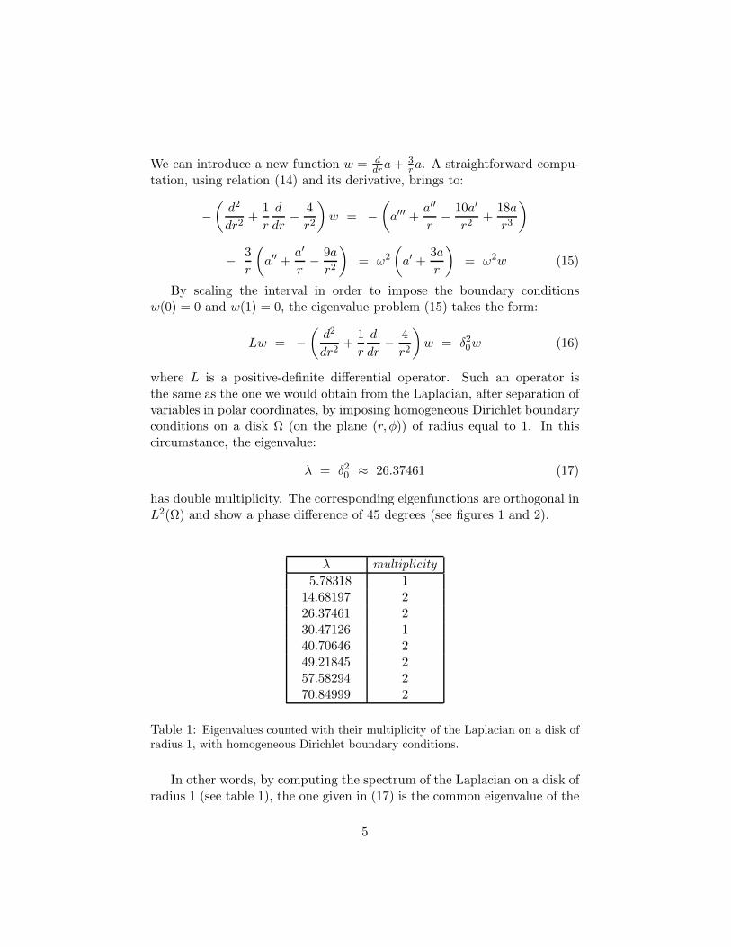
λ = δ20 ≈ 26.37461 (17)

has double multiplicity. The corresponding eigenfunctions are orthogonal inL2(Ω) and show a phase difference of 45 degrees (see figures 1 and 2).

λ multiplicity

5.78318 114.68197 226.37461 230.47126 140.70646 249.21845 257.58294 270.84999 2

Table 1: Eigenvalues counted with their multiplicity of the Laplacian on a disk ofradius 1, with homogeneous Dirichlet boundary conditions.

In other words, by computing the spectrum of the Laplacian on a disk ofradius 1 (see table 1), the one given in (17) is the common eigenvalue of the

5

fourth and the fifth eigenfunctions. Note that there are no eigenvalues withmultiplicity greater than 2. We also note that Φ = 0 at the boundary of Ω.These simple observations will be of primary importance in the discussionto follow.

Figure 1: Signature of the first 8 eigenfunctions of the Laplace’s equation on adisk. The first eigenfunction (w1) does not change sign. The two successive ones(w2 and w3) display a phase difference of 90 degrees. Then, we have w4 and w5

with a phase difference of 45 degrees. The next one (w6) is a single multiplicityeigenfunction, while the last ones (w7 and w8) have a phase difference of 30 degrees.

Figure 2: Solutions of the wave equation on a disk are obtained by linearly combin-ing independent eigenfunction having the same eigenvalue. For example, a completerotation is simulated through the sequence: w4, w5,−w4,−w5, w4, w5,−w4,−w5.Intermediate situations are obtained by taking w4 cos ct

√λ + w5 sin ct

√λ, with

0 ≤ ct√λ ≤ 2π, where λ is the common eigenvalue.

3 The Toroid Case

We are ready to study the 3-D case. In cylindrical coordinates (r, z, φ), weconsider the potentials:

A =1

c

(

a(t, r, z), b(t, r, z), 0)

Φ = −(

∂A

∂r+

A

r+

∂B

∂z

)

(18)

6

where a and b are functions to be computed, while A and B are their primi-tives with respect to the time variable. In this context, the Lorenz condition(6) turns out to be automatically satisfied. The functions a and b will de-scribe the time evolution, in a certain region Ω of the plane (r, z), of arotating wave similar to the one studied in the previous section (differentlyfrom the previous case, Ω is now vertically oriented). Since there is no de-pendance on φ, the solution is automatically extended to a toroid Σ, havingsection Ω, with the axis parallel to the z-axis.

From the potentials we deduce the electromagnetic fields (see (5)):

E =(

− ∂Φ

∂r− 1

c2∂a

∂t, − ∂Φ

∂z− 1

c2∂b

∂t, 0

)

B =1

c2

(

0, 0,∂b

∂r− ∂a

∂z

)

(19)

We now require E and B to satisfy the whole set of Maxwell equations (inalternative, we get the same conclusions by imposing (7) and (8)). Theresult is the following system:

1

c2∂2a

∂t2=

∂2a

∂z2+

∂

∂r

(

∂a

∂r+

a

r

)

(20)

1

c2∂2b

∂t2=

∂2b

∂z2+

∂2b

∂r2+

1

r

∂b

∂r(21)

We can couple a and b through the boundary condition:

∂a

∂z=

∂b

∂r(22)

which amounts to ask B = c−1curlA = 0 at the contour of Ω. Thefield E is tangential to the same boundary. As a matter of fact, thanks to(18)-(20)-(21), one can write:

E =

(

∂

∂z

(∂A

∂z− ∂B

∂r

)

, − 1

r

∂

∂r

(

r∂A

∂z− r

∂B

∂r

)

, 0

)

(23)

which means that E is orthogonal to the gradient of r(

∂∂zA− ∂

∂rB)

. Since

(22) is valid for any t, such a gradient is orthogonal to the boundary of Ω,showing that E is tangential.

Note that now the set Ω is not going to be a circle. As done in Ref. [1],section 5.4, we set y = r − η. The domain Ω will be centered at the point(η, 0), where η > 0 is large enough to avoid intersection of Ω with the z-axis.The quantity 2η is related to the major diameter of the toroid.

7

By differentiating the first equation with respect to z and the second onewith respect to y, one gets:

1

c2∂2u

∂t2=

∂2u

∂z2+

∂

∂y

(

∂u

∂y+

u

y + η

)

1

c2∂2v

∂t2=

∂2v

∂z2+

∂

∂y

(

∂v

∂y+

v

y + η

)

(24)

where we took u = ∂∂za and v = ∂

∂r b =∂∂y b, with u − v = 0 on ∂Ω. Fur-

thermore, with the substitutions u = u√y + η, v = v

√y + η, one obtains:

1

c2∂2u

∂t2=

∂2u

∂z2+

∂2u

∂y2− 3

4

u

(y + η)2

1

c2∂2v

∂t2=

∂2v

∂z2+

∂2v

∂y2− 3

4

v

(y + η)2

(25)

to be solved in Ω, with the boundary condition: u− v = 0.

Similarly to the case examined in section 2, we look for solutions associ-ated to the second mode (k = 2 in (13)) with respect to the angle of rotation.According to the captions of figures 1 and 2, the functions u and v shouldhave a phase difference of 45 degrees (this property is now qualitative, sinceΩ is not a perfect disk). We fix the area of Ω to be equal to π. For η tendingto infinity, the set Ω converges to a circle of radius 1 and the electromagneticfields coincide with those given in (9) for ω = δ0.

We proceed by introducing a new unknown w = u− v and by taking thedifference of the two equations in (25). Then, we can get rid of the timevariable and pass to the stationary eigenvalue problem:

Lw = − ∂2w

∂z2− ∂2w

∂y2+

3

4

w

(y + η)2= λw in Ω

w = 0 on ∂Ω

(26)

Thus, we would like λ > 0 to be an eigenvalue of the positive-definite differ-ential operator: L = − ∂2

∂z2− ∂2

∂y2+ 3

4(y + η)−2, with homogeneous Dirichletboundary conditions. In addition, since we want two independent eigen-functions with a difference of phase of 45 degrees, the multiplicity of λ mustbe equal to 2. This implicitly defines Ω. More precisely, we require thatλ = λ4 = λ5, where λ4 and λ5 are the eigenvalues of the fourth and the fifth

8

eigenfunctions, w4 and w5, of L on Ω. In order to preserve energy, theseeigenfunctions will be normalized in L2(Ω). In this way, by setting:

u(t, y, z) − v(t, y, z) = w4(y, z) sin(ct√λ) + w5(y, z) cos(ct

√λ) (27)

one gets a full solution of the system (25). We can finally recover the elec-tromagnetic fields by the expressions (see (23)):

E =1

c√λ

(

∂

∂z

(−w4 cos ζ + w5 sin ζ√y + η

)

,

−1√y + η

∂

∂y

(

(−w4 cos ζ +w5 sin ζ)√y + η

)

, 0

)

B =1

c2

(

0, 0,w4 sin ζ + w5 cos ζ√

y + η

)

(28)

with ζ = ct√λ. As in figure 2, by varying the parameter t, we can simulate

a rotating object.

Of course, we could also take into consideration the case k > 2 (see the2-D analog (13)) by studying the behavior of eigenvalues with higher mag-nitude. The search, in this case, should be addressed to the determinationof couples of independent eigenfunctions sharing the same eigenvalue. Wethink this is a viable option, although, in order to maintain the discussionat a simple level, we will not analyze this extension.

We now define Σ = Ω × [0, 2π[, in order to get a 3-D solution not de-pending on φ. In fluid dynamics this structure is known as vortex ring (seefor instance Ref. [2], section 7.2, or [3]). On the surface of Σ, field E istangential and B is zero. At every point inside Σ, the time average dur-ing a period of oscillation, of both E and B, is zero (see the animations inRef. [5]).

We would like to know more about the shape of Σ. Considering that notall the sets Ω are such that λ4 and λ5 are equal, we can use this property inorder to determine the right domain. This problem admits however infinitesolutions. In the next section we discuss how to find numerically somesuitable configurations.

4 On the Optimal Shape of Ω

We first observe that, among the sets with fixed area equal to π, the circleof radius 1, minimizes the eigenvalues of the Laplacian with homogeneous

9

Dirichlet boundary conditions (see for instance Ref. [7]). Due to symmetryarguments, all the eigenvalues related to the angular modes have multi-plicity 2 (see table 1 and figure 1). The eigenfunctions are supposed tobe orthogonal and normalized in L2(Ω). Then, the normal derivative ofthe eigenfunction related to the lowest eigenvalue, has constant value onthe boundary of the disk. Similarly, the sum of the squares of the normalderivatives of the eigenfunctions related to the second and the third eigen-values, is constant along the boundary. The same is true for all the couplesof eigenfunctions relative to other eigenvalues with double multiplicity (thefourth and the fifth, for example).

We now replace the Laplacian by the new elliptic operator L = − ∂2

∂z2−

∂2

∂y2+34 (y+η)−2 (see (26)), with homogeneous Dirichlet boundary conditions.

We are concerned with finding a set Ω, with area equal to π, such that thefourth and the fifth eigenvalues, λ4 and λ5, of L are coincident. Thanks to(27), this allows us to determine solutions of a wave-type equation, rotatinginside Ω with an angular velocity proportional to

√λ, where λ = λ4 = λ5. In

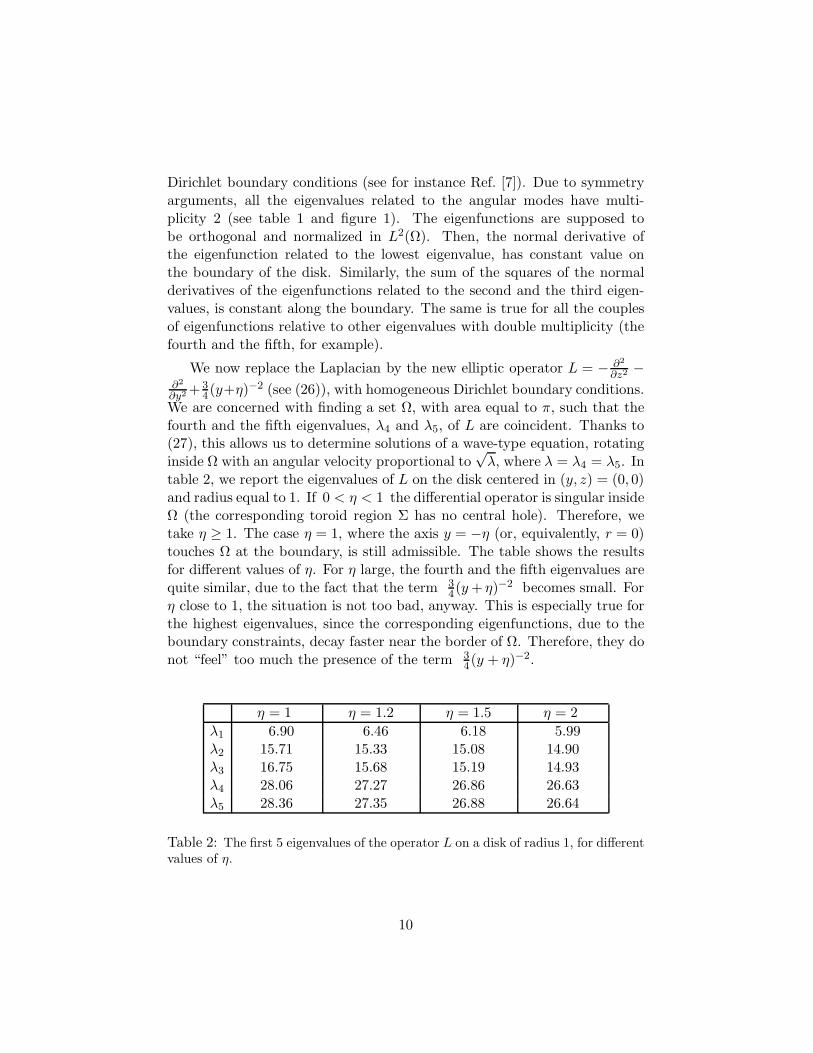
table 2, we report the eigenvalues of L on the disk centered in (y, z) = (0, 0)and radius equal to 1. If 0 < η < 1 the differential operator is singular insideΩ (the corresponding toroid region Σ has no central hole). Therefore, wetake η ≥ 1. The case η = 1, where the axis y = −η (or, equivalently, r = 0)touches Ω at the boundary, is still admissible. The table shows the resultsfor different values of η. For η large, the fourth and the fifth eigenvalues arequite similar, due to the fact that the term 3

4(y+ η)−2 becomes small. Forη close to 1, the situation is not too bad, anyway. This is especially true forthe highest eigenvalues, since the corresponding eigenfunctions, due to theboundary constraints, decay faster near the border of Ω. Therefore, they donot “feel” too much the presence of the term 3

4(y + η)−2.

η = 1 η = 1.2 η = 1.5 η = 2

λ1 6.90 6.46 6.18 5.99λ2 15.71 15.33 15.08 14.90λ3 16.75 15.68 15.19 14.93λ4 28.06 27.27 26.86 26.63λ5 28.36 27.35 26.88 26.64

Table 2: The first 5 eigenvalues of the operator L on a disk of radius 1, for differentvalues of η.

10

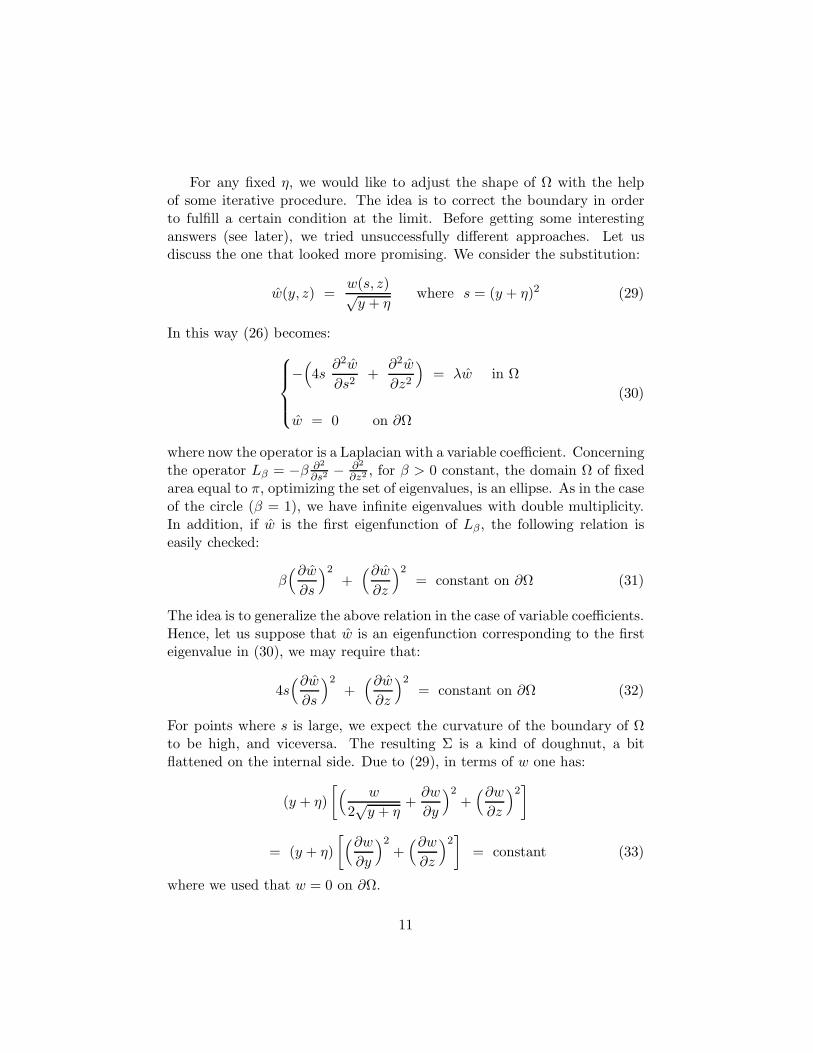
For any fixed η, we would like to adjust the shape of Ω with the helpof some iterative procedure. The idea is to correct the boundary in orderto fulfill a certain condition at the limit. Before getting some interestinganswers (see later), we tried unsuccessfully different approaches. Let usdiscuss the one that looked more promising. We consider the substitution:

w(y, z) =w(s, z)√y + η

where s = (y + η)2 (29)

In this way (26) becomes:

−(

4s∂2w

∂s2+

∂2w

∂z2

)

= λw in Ω

w = 0 on ∂Ω

(30)

where now the operator is a Laplacian with a variable coefficient. Concerningthe operator Lβ = −β ∂2

∂s2− ∂2

∂z2, for β > 0 constant, the domain Ω of fixed

area equal to π, optimizing the set of eigenvalues, is an ellipse. As in the caseof the circle (β = 1), we have infinite eigenvalues with double multiplicity.In addition, if w is the first eigenfunction of Lβ, the following relation iseasily checked:

β(∂w

∂s

)2+

(∂w

∂z

)2= constant on ∂Ω (31)

The idea is to generalize the above relation in the case of variable coefficients.Hence, let us suppose that w is an eigenfunction corresponding to the firsteigenvalue in (30), we may require that:

4s(∂w

∂s

)2+

(∂w

∂z

)2= constant on ∂Ω (32)

For points where s is large, we expect the curvature of the boundary of Ωto be high, and viceversa. The resulting Σ is a kind of doughnut, a bitflattened on the internal side. Due to (29), in terms of w one has:

(y + η)

[

( w

2√y + η

+∂w

∂y

)2+

(∂w

∂z

)2]

= (y + η)

[

(∂w

∂y

)2+

(∂w

∂z

)2]

= constant (33)

where we used that w = 0 on ∂Ω.

11

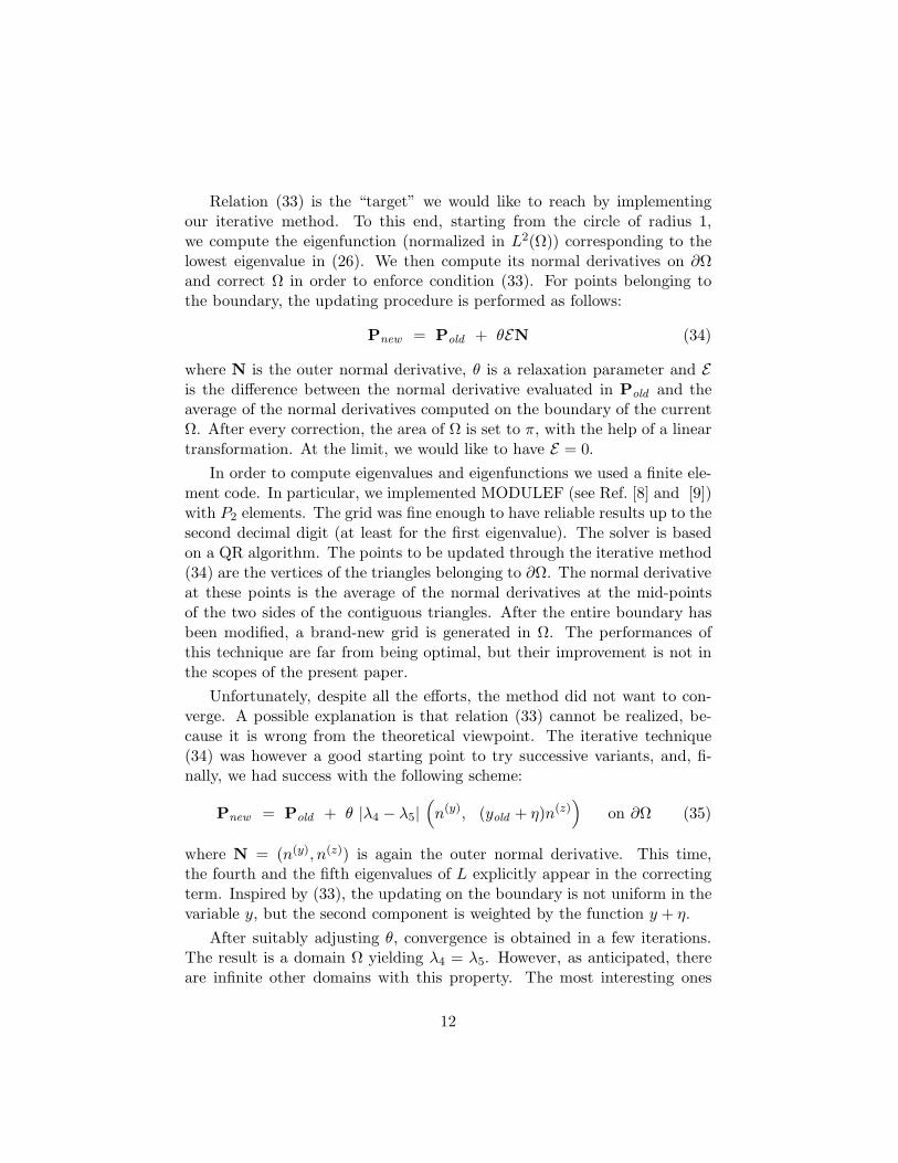
Relation (33) is the “target” we would like to reach by implementingour iterative method. To this end, starting from the circle of radius 1,we compute the eigenfunction (normalized in L2(Ω)) corresponding to thelowest eigenvalue in (26). We then compute its normal derivatives on ∂Ωand correct Ω in order to enforce condition (33). For points belonging tothe boundary, the updating procedure is performed as follows:

Pnew = Pold + θEN (34)

where N is the outer normal derivative, θ is a relaxation parameter and Eis the difference between the normal derivative evaluated in Pold and theaverage of the normal derivatives computed on the boundary of the currentΩ. After every correction, the area of Ω is set to π, with the help of a lineartransformation. At the limit, we would like to have E = 0.

In order to compute eigenvalues and eigenfunctions we used a finite ele-ment code. In particular, we implemented MODULEF (see Ref. [8] and [9])with P2 elements. The grid was fine enough to have reliable results up to thesecond decimal digit (at least for the first eigenvalue). The solver is basedon a QR algorithm. The points to be updated through the iterative method(34) are the vertices of the triangles belonging to ∂Ω. The normal derivativeat these points is the average of the normal derivatives at the mid-pointsof the two sides of the contiguous triangles. After the entire boundary hasbeen modified, a brand-new grid is generated in Ω. The performances ofthis technique are far from being optimal, but their improvement is not inthe scopes of the present paper.

Unfortunately, despite all the efforts, the method did not want to con-verge. A possible explanation is that relation (33) cannot be realized, be-cause it is wrong from the theoretical viewpoint. The iterative technique(34) was however a good starting point to try successive variants, and, fi-nally, we had success with the following scheme:

Pnew = Pold + θ |λ4 − λ5|(

n(y), (yold + η)n(z))

on ∂Ω (35)

where N = (n(y), n(z)) is again the outer normal derivative. This time,the fourth and the fifth eigenvalues of L explicitly appear in the correctingterm. Inspired by (33), the updating on the boundary is not uniform in thevariable y, but the second component is weighted by the function y + η.

After suitably adjusting θ, convergence is obtained in a few iterations.The result is a domain Ω yielding λ4 = λ5. However, as anticipated, thereare infinite other domains with this property. The most interesting ones

12

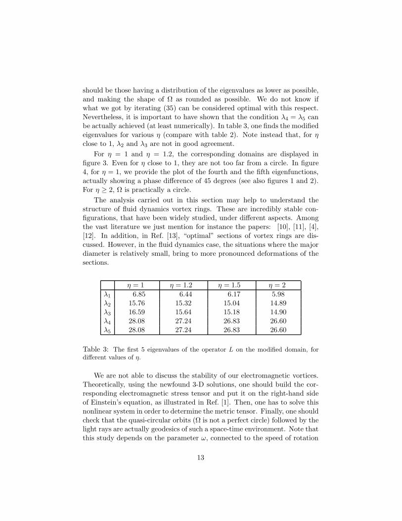
should be those having a distribution of the eigenvalues as lower as possible,and making the shape of Ω as rounded as possible. We do not know ifwhat we got by iterating (35) can be considered optimal with this respect.Nevertheless, it is important to have shown that the condition λ4 = λ5 canbe actually achieved (at least numerically). In table 3, one finds the modifiedeigenvalues for various η (compare with table 2). Note instead that, for ηclose to 1, λ2 and λ3 are not in good agreement.

For η = 1 and η = 1.2, the corresponding domains are displayed infigure 3. Even for η close to 1, they are not too far from a circle. In figure4, for η = 1, we provide the plot of the fourth and the fifth eigenfunctions,actually showing a phase difference of 45 degrees (see also figures 1 and 2).For η ≥ 2, Ω is practically a circle.

The analysis carried out in this section may help to understand thestructure of fluid dynamics vortex rings. These are incredibly stable con-figurations, that have been widely studied, under different aspects. Amongthe vast literature we just mention for instance the papers: [10], [11], [4],[12]. In addition, in Ref. [13], “optimal” sections of vortex rings are dis-cussed. However, in the fluid dynamics case, the situations where the majordiameter is relatively small, bring to more pronounced deformations of thesections.

η = 1 η = 1.2 η = 1.5 η = 2

λ1 6.85 6.44 6.17 5.98λ2 15.76 15.32 15.04 14.89λ3 16.59 15.64 15.18 14.90λ4 28.08 27.24 26.83 26.60λ5 28.08 27.24 26.83 26.60

Table 3: The first 5 eigenvalues of the operator L on the modified domain, fordifferent values of η.

We are not able to discuss the stability of our electromagnetic vortices.Theoretically, using the newfound 3-D solutions, one should build the cor-responding electromagnetic stress tensor and put it on the right-hand sideof Einstein’s equation, as illustrated in Ref. [1]. Then, one has to solve thisnonlinear system in order to determine the metric tensor. Finally, one shouldcheck that the quasi-circular orbits (Ω is not a perfect circle) followed by thelight rays are actually geodesics of such a space-time environment. Note thatthis study depends on the parameter ω, connected to the speed of rotation

13

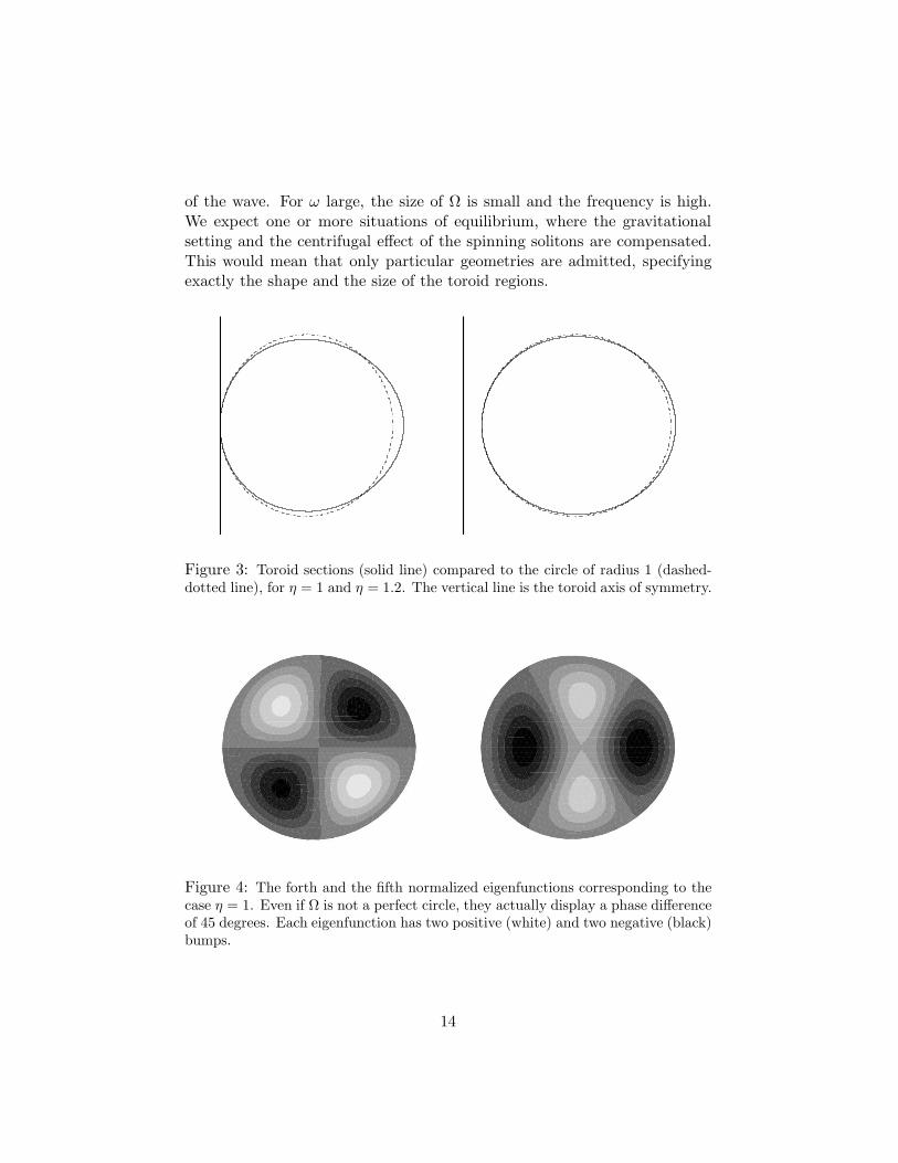
of the wave. For ω large, the size of Ω is small and the frequency is high.We expect one or more situations of equilibrium, where the gravitationalsetting and the centrifugal effect of the spinning solitons are compensated.This would mean that only particular geometries are admitted, specifyingexactly the shape and the size of the toroid regions.

Figure 3: Toroid sections (solid line) compared to the circle of radius 1 (dashed-dotted line), for η = 1 and η = 1.2. The vertical line is the toroid axis of symmetry.

Figure 4: The forth and the fifth normalized eigenfunctions corresponding to thecase η = 1. Even if Ω is not a perfect circle, they actually display a phase differenceof 45 degrees. Each eigenfunction has two positive (white) and two negative (black)bumps.

14

Of course, what we just said above turns out to be very hard to prove,both theoretically and computationally. Note that we are also omitting astationary component of the electromagnetic fields, introduced in Ref. [1],which should provide charge and mass to the particle model. We do notinsist further on this topic and we address the reader to Ref. [1] for additionalinformation.

5 Hill’s Type Vortices

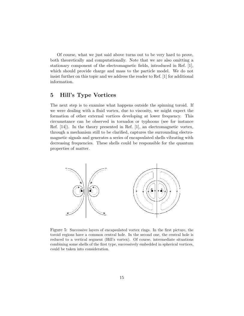
The next step is to examine what happens outside the spinning toroid. Ifwe were dealing with a fluid vortex, due to viscosity, we might expect theformation of other external vortices developing at lower frequency. Thiscircumstance can be observed in tornados or typhoons (see for instanceRef. [14]). In the theory presented in Ref. [1], an electromagnetic vortex,through a mechanism still to be clarified, captures the surrounding electro-magnetic signals and generates a series of encapsulated shells vibrating withdecreasing frequencies. These shells could be responsible for the quantumproperties of matter.

Figure 5: Successive layers of encapsulated vortex rings. In the first picture, thetoroid regions have a common central hole. In the second one, the central hole isreduced to a vertical segment (Hill’s vortex). Of course, intermediate situationscombining some shells of the first type, successively embedded in spherical vortices,could be taken into consideration.

15

Basically, there are two possible ways in which external ring vorticesmay develop. As the first picture of figure 5 shows, we may have a seriesof successive toroid structures, where all the fluid stream-lines pass througha common central hole. This situation is difficult to analyze, since we haveno idea of the shape of these regions and the location of the primary vortexinside them. In practice, there are too many degrees of freedom to workwith.

The other situation (second picture of figure 5) is more affordable. Itrepresents an Hill’s spherical vortex (see Ref. [2], section 7.2, and Ref. [15]for some computational results), successively surrounded by other sphericallayers. Thus, we now know exactly the shape of these structures. We justhave to find the location (and the relative size) of the primary toroid vortexinside the most internal sphere. This research will lead us to interestingconclusions.

Figure 6: Sections of spherical vortices.

We start by considering the domain A in figure 6. We set the radius equalto 1, so that the area is π/2. We solve in Ω = A the eigenvalue problem (26),

involving the operator L = − ∂2

∂z2 −∂2

∂r2 +3

4r2 (r = y + η with η = 0). In thefirst column of table 4, we report the approximated eigenvalues, obtainedby discretization with the finite element method. As the reader can notice,the fourth and the fifth eigenvalues are not coincident. Therefore, for a

16

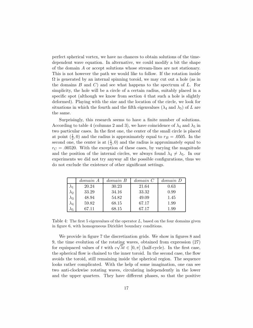
perfect spherical vortex, we have no chances to obtain solutions of the time-dependent wave equation. In alternative, we could modify a bit the shapeof the domain A or accept solutions whose stream-lines are not stationary.This is not however the path we would like to follow. If the rotation insideΩ is generated by an internal spinning toroid, we may cut out a hole (as inthe domains B and C) and see what happens to the spectrum of L. Forsimplicity, the hole will be a circle of a certain radius, suitably placed in aspecific spot (although we know from section 4 that such a hole is slightlydeformed). Playing with the size and the location of the circle, we look forsituations in which the fourth and the fifth eigenvalues (λ4 and λ5) of L arethe same.

Surprisingly, this research seems to have a finite number of solutions.According to table 4 (columns 2 and 3), we have coincidence of λ4 and λ5 intwo particular cases. In the first one, the center of the small circle is placedat point (12 , 0) and the radius is approximately equal to rB = .0505. In thesecond one, the center is at (14 , 0) and the radius is approximately equal torC = .00520. With the exception of these cases, by varying the magnitudeand the position of the internal circles, we always found λ4 6= λ5. In ourexperiments we did not try anyway all the possible configurations, thus wedo not exclude the existence of other significant settings.

domain A domain B domain C domain D

λ1 20.24 30.23 21.64 0.63λ2 33.29 34.16 33.32 0.99λ3 48.94 54.82 49.09 1.45λ4 59.82 68.15 67.17 1.99λ5 67.11 68.15 67.17 1.99

Table 4: The first 5 eigenvalues of the operator L, based on the four domains givenin figure 6, with homogeneous Dirichlet boundary conditions.

We provide in figure 7 the discretization grids. We show in figures 8 and9, the time evolution of the rotating waves, obtained from expression (27)for equispaced values of t with c

√λt ∈ [0, π] (half-cycle). In the first case,

the spherical flow is chained to the inner toroid. In the second case, the flowavoids the toroid, still remaining inside the spherical region. The sequencelooks rather complicated. With the help of some imagination, one can seetwo anti-clockwise rotating waves, circulating independently in the lowerand the upper quarters. They have different phases, so that the positive

17

(white) bumps and the negative (black) ones, alternately merge to form asingle protuberance situated near the center. The pictures only show halfof the cycle. Then, the sequence restarts with the two colors interchanged.The corresponding animations can be found in Ref. [5] (click related papers).

We point out once again that we are dealing with electromagnetic waves.Therefore, we should ask ourselves what happens to the vector fields. Ourplots actually show the evolution of the function ∂

∂r b − ∂∂za, where A =

c−1(a, b, 0) is the vector potential. Using (19), (23) and (28), one thencomputes E and B. We discover that, at each point, when time passes, thetips of the arrows of the electric field turn around, describing elliptic orbits(see the animations in Ref. [5] in the case of a circle). The average of Eduring a cycle is zero. The frequency of rotation is globally the same, but,depending on the point, it is associated with a different phase, so that thegeneral framework seems quite unorganized.

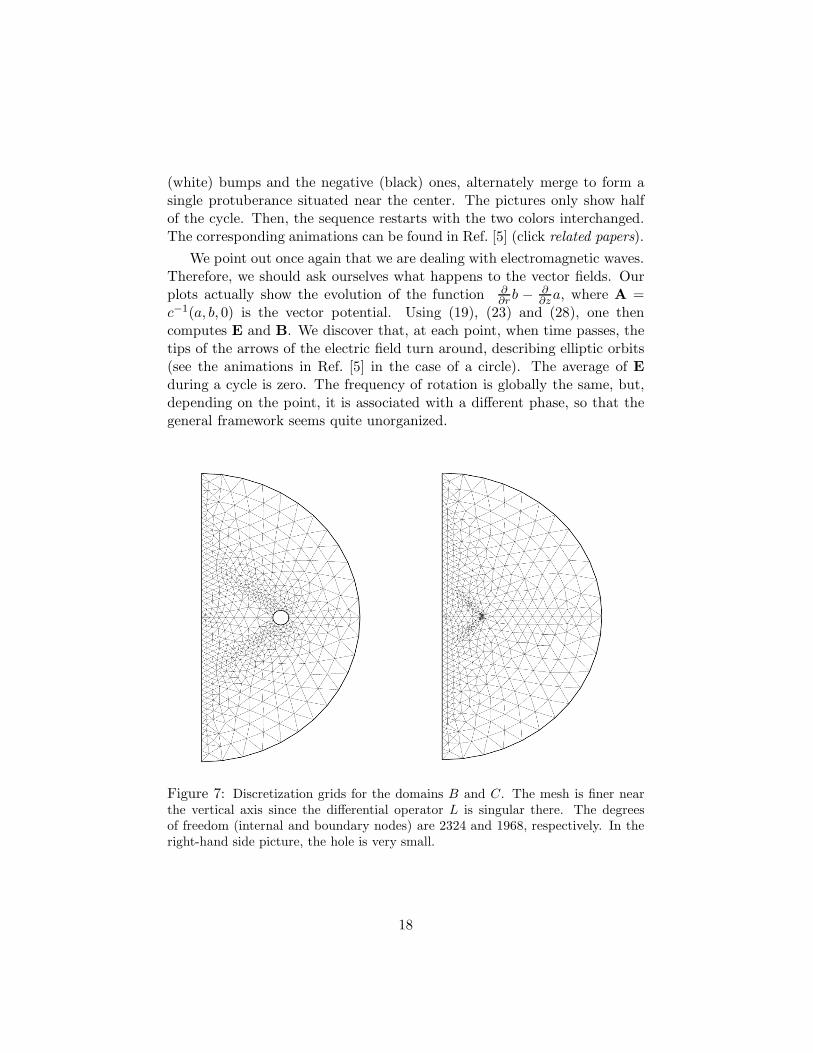
Figure 7: Discretization grids for the domains B and C. The mesh is finer nearthe vertical axis since the differential operator L is singular there. The degreesof freedom (internal and boundary nodes) are 2324 and 1968, respectively. In theright-hand side picture, the hole is very small.

18

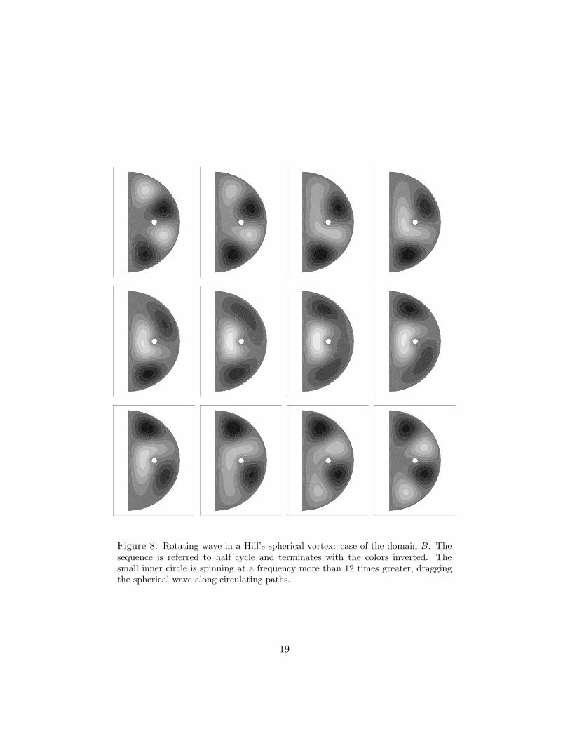
Figure 8: Rotating wave in a Hill’s spherical vortex: case of the domain B. Thesequence is referred to half cycle and terminates with the colors inverted. Thesmall inner circle is spinning at a frequency more than 12 times greater, draggingthe spherical wave along circulating paths.

19

Figure 9: Rotating wave in a Hill’s spherical vortex: case of the domain C. Thetiny inner circle (hardly visible in the pictures) is spinning at a frequency about120 times greater. The behavior is qualitatively the same as in figure 8, but nowthe wave do not pass between the circle and the vertical axis.

20

From the size of the hole, we can estimate the frequency of rotation ofthe internal toroid regions. Such a frequency is proportional to the squareroot of a suitable eigenvalue. We take the value

√26.37 ≈ 5.135, that, ac-

cording to table 1, is the square root of the eigenvalue corresponding to thefourth and the fifth eigenfunctions, for a circle of radius 1. Afterwards, byscaling, we get the frequencies on the reduced circles: 5.135/rB ≈ 101.68and 5.135/rC ≈ 987.5. Thus, the ratio between the frequencies of the in-ner spinning rings and the spherical vortices are given by (see table 4, thelast line of the second and the third columns): 101.68/

√68.15 ≈ 12.31 and

987.5/√67.17 ≈ 120.48, respectively. Note that these numbers may be af-

fected by rounding errors (in particular, we expect an error bound of ±0.005in the computation of the eigenvalues), therefore they should be taken witha little caution. Of course, more trustable results can be obtained with afiner mesh.

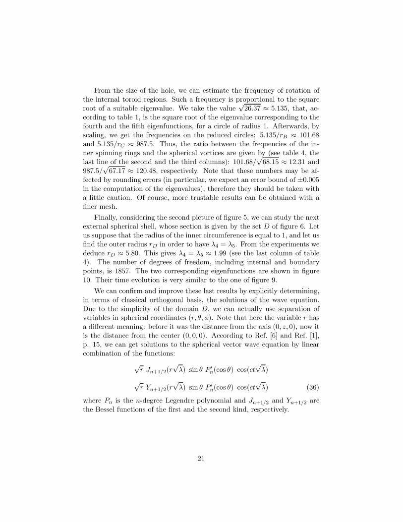
Finally, considering the second picture of figure 5, we can study the nextexternal spherical shell, whose section is given by the set D of figure 6. Letus suppose that the radius of the inner circumference is equal to 1, and let usfind the outer radius rD in order to have λ4 = λ5. From the experiments wededuce rD ≈ 5.80. This gives λ4 = λ5 ≈ 1.99 (see the last column of table4). The number of degrees of freedom, including internal and boundarypoints, is 1857. The two corresponding eigenfunctions are shown in figure10. Their time evolution is very similar to the one of figure 9.

We can confirm and improve these last results by explicitly determining,in terms of classical orthogonal basis, the solutions of the wave equation.Due to the simplicity of the domain D, we can actually use separation ofvariables in spherical coordinates (r, θ, φ). Note that here the variable r hasa different meaning: before it was the distance from the axis (0, z, 0), now itis the distance from the center (0, 0, 0). According to Ref. [6] and Ref. [1],p. 15, we can get solutions to the spherical vector wave equation by linearcombination of the functions:

√r Jn+1/2(r

√λ) sin θ P ′

n(cos θ) cos(ct√λ)

√r Yn+1/2(r

√λ) sin θ P ′

n(cos θ) cos(ct√λ) (36)

where Pn is the n-degree Legendre polynomial and Jn+1/2 and Yn+1/2 arethe Bessel functions of the first and the second kind, respectively.

21

Figure 10: Two independent eigenfunctions in the case of the domain D, forλ4 = λ5 ≈ 1.9639.

We are concerned with the cases n = 1 and n = 4. For these val-ues, the functions in (36) have, with respect to the azimuthal variable θ,one single bump or 4 consecutive bumps, respectively (see figure 10). Asa matter of fact, we have: sin θP ′

1(cos θ) = sin θ and sin θP ′

4(cos θ) =52 sin θ cos θ(7 cos

2 θ − 3). Regarding instead the radial variable r, we wouldlike to find suitable linear combinations of the functions in (36), in order toimpose homogeneous Dirichlet boundary conditions at r = 1 and r = rD.In agreement with the results obtained by implementing the finite elementmethod, playing with the zeros of Bessel functions, yields:

λ = λ4 = λ5 ≈ 1.9639 and rD ≈ 5.839 (37)

These data are now more accurate. The correct assemblage of the radialbasis functions can be seen in figure 11. The first picture shows a linearcombination of J3/2 and Y3/2 (n = 1), the second one a linear combinationof J9/2 and Y9/2 (n = 4). Up to multiplicative constants, this setting isunique if we impose the boundary conditions at the endpoints of the sameinterval [1, rD]. In a similar way, we can also update the values of table 4

22

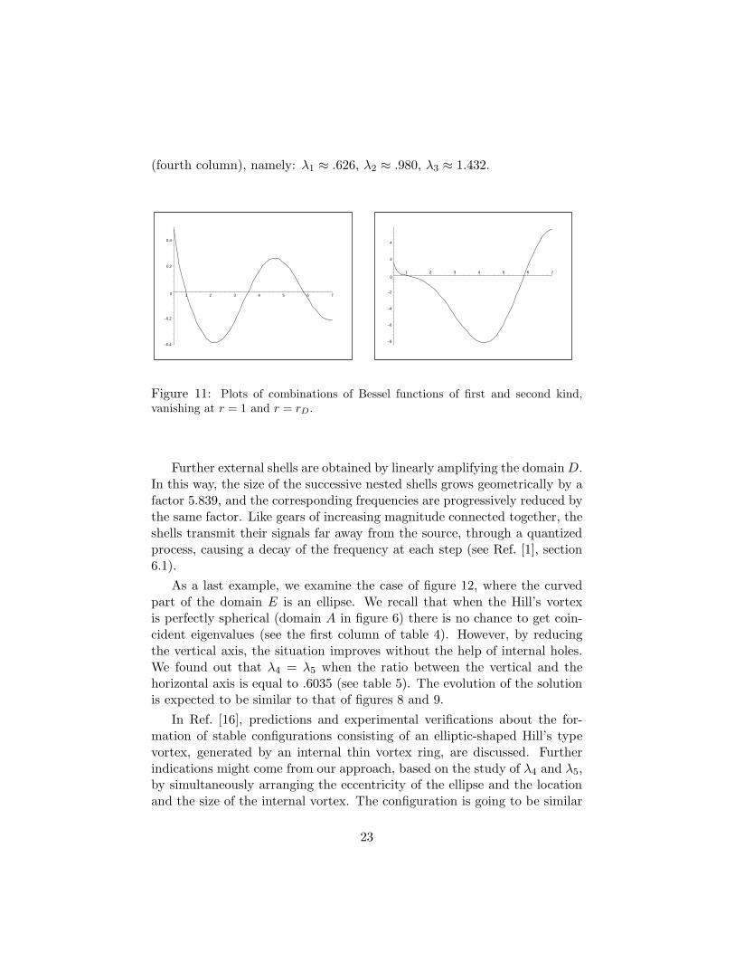
(fourth column), namely: λ1 ≈ .626, λ2 ≈ .980, λ3 ≈ 1.432.

–0.4

–0.2

0

0.2

0.4

1 2 3 4 5 6 7

–8

–6

–4

–2

0

2

4

1 2 3 4 5 6 7

Figure 11: Plots of combinations of Bessel functions of first and second kind,vanishing at r = 1 and r = rD.

Further external shells are obtained by linearly amplifying the domainD.In this way, the size of the successive nested shells grows geometrically by afactor 5.839, and the corresponding frequencies are progressively reduced bythe same factor. Like gears of increasing magnitude connected together, theshells transmit their signals far away from the source, through a quantizedprocess, causing a decay of the frequency at each step (see Ref. [1], section6.1).

As a last example, we examine the case of figure 12, where the curvedpart of the domain E is an ellipse. We recall that when the Hill’s vortexis perfectly spherical (domain A in figure 6) there is no chance to get coin-cident eigenvalues (see the first column of table 4). However, by reducingthe vertical axis, the situation improves without the help of internal holes.We found out that λ4 = λ5 when the ratio between the vertical and thehorizontal axis is equal to .6035 (see table 5). The evolution of the solutionis expected to be similar to that of figures 8 and 9.

In Ref. [16], predictions and experimental verifications about the for-mation of stable configurations consisting of an elliptic-shaped Hill’s typevortex, generated by an internal thin vortex ring, are discussed. Furtherindications might come from our approach, based on the study of λ4 and λ5,by simultaneously arranging the eccentricity of the ellipse and the locationand the size of the internal vortex. The configuration is going to be similar

23

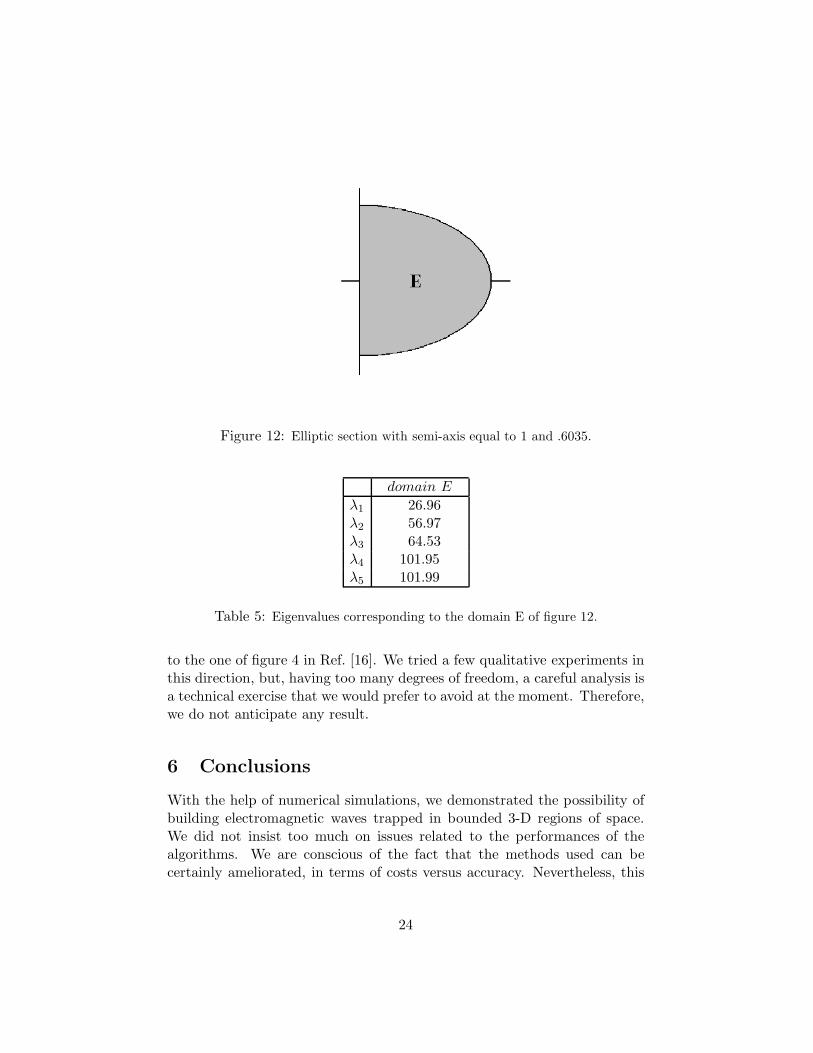
Figure 12: Elliptic section with semi-axis equal to 1 and .6035.

domain E

λ1 26.96λ2 56.97λ3 64.53λ4 101.95λ5 101.99

Table 5: Eigenvalues corresponding to the domain E of figure 12.

to the one of figure 4 in Ref. [16]. We tried a few qualitative experiments inthis direction, but, having too many degrees of freedom, a careful analysis isa technical exercise that we would prefer to avoid at the moment. Therefore,we do not anticipate any result.

6 Conclusions

With the help of numerical simulations, we demonstrated the possibility ofbuilding electromagnetic waves trapped in bounded 3-D regions of space.We did not insist too much on issues related to the performances of thealgorithms. We are conscious of the fact that the methods used can becertainly ameliorated, in terms of costs versus accuracy. Nevertheless, this

24

was not our primary concern.

We think that the results we got may have a general validity indepen-dently on the field of applications. In fact, the approach we followed, basedon the determination of periodic solutions to the wave equation through theanalysis of certain eigenvalues of a suitable differential operator, may beapplied in several circumstances. For example, as an alternative, this tech-nique may be employed in fluid dynamics (for stable periodic flows), wherecomputations are usually carried out by discretizing the equations by sometime-advancing procedure. However, the meaning of the results obtainedhere is deeper, since they are related to the approximation of a completesystem of hyperbolic equations (namely the Maxwell’s equations) and notjust to the detection of the flow-field. As a matter of fact, the informationcarried by our waves is not a scalar density field, but it consists of two sep-arated vector fields: the electric and the magnetic ones. These can be fullyexpressed by the relations in (28).

A recent subject of research, that could benefit from our investigation,is the detection of quantum vortex rings in superfluid helium (the literaturein the field is very rich, see for instance Ref. [17] for a general overview).Note that, in liquid helium, the thickness of these rings is on the order ofa few Angstroms. Other related topics might be the study of ball lightningphenomena (see for instance Ref. [18] and Ref. [19]) or ring nebulae andtheir halos (see for instance Ref. [20]).

Our analysis might inspire interesting applications, that at the momentwe are unable to predict. Indeed, we showed that it is possible to detect 3-Dregions of space, where an electromagnetic wave, suitably supplied throughthe boundary, can freely travel without bouncing off the walls. Moreover, wealso explained how to build these regions. We are not enough experiencedin the field of applications to find an employment for such resonant boxes,but this paper may suggest to some interested reader how to use them tocreate new tools or improve existing ones.

Finally, we recall that the stability of these structures is a consequenceof gravitational modifications of the space-time generated by the movementof the wave itself, according to Einstein’s equation. In fact, the wave trav-els like a fluid, along closed stream-lines, that turn out to be geodesics ofsuch a modified geometry (see also Ref. [21]). Thus, in the electrodynamicframework, a complete analysis of stability depends on the resolution of acomplex relativistic problem. Nevertheless, we hope that the simple inves-tigation carried out in this paper may represent a step ahead towards abetter comprehension of the mechanism of vortex formation, whatever the

25

constituents are (fields or real matter).

References

[1] D. Funaro, Electromagnetism and the Structure of Matter (World Sci-entific, Singapore, 2008).

[2] G.K. Batchelor, An Introduction to Fluid Dynamics(Cambridge Univ.Press, 1967).

[3] T.T. Lim and T.B. Nickels, Vortex rings, Fluid Vortices , ed. S. I. Green(Kluwer Academic, NY, 1995).

[4] K. Shariff and A. Leonard, Vortex rings,Annual Rev. Fluid Mech. 24,p.235 (1992).

[5] http://cdm.unimo.it/home/matematica/funaro.daniele/phys.htm

[6] G.N. Watson, A Treatise on the Theory of Bessel Functions (CambridgeUniversity Press, 1944).

[7] A. Henrot and M. Pierre, Variation et Optimisation de Formes: Une

Analyse Geometrique (Springer-Verlag, Heidelberg, 2005).

[8] Modulef Installation Page, http://www-rocq.inria.fr/modulef

[9] P. Laug and P.L. George, Normes d’utilisation et de programmation,Guide MODULEF N. 2 ( INRIA, Paris-Rocquencourt,1992).

[10] T.J. Maxworthy, The structure and stability of vortex rings, Journal ofFluid Mechanics 51, p.15 (1972).

[11] D.I. Pullin, Vortex ring formation at tube and orifice openings, Phys.Fluids 22, p.401 (1979).

[12] S.L. Wakelin and N. Riley, On the formation of vortex rings and pairsof vortex rings, Journal of Fluid Mechanics 332, p.121 (1997).

[13] P.F. Linden and J.S. Turner, The formation of ‘optimal’ vortex rings,and the efficiency of propulsion devices, Journal of Fluid Mechanics

427, p.61 (2001).

[14] H.C. Kuo, L.Y. Lin, C.P. Chang and R.T. Williams, The formation ofconcentric vorticity structures in typhoons, J. Atmos. Sci. 61, p.2722(2004).

26

[15] A. R. Elcrat, B. Fornberg and K.G. Miller, Some steady axissymmet-ric vortex flows past a sphere, Journal of Fluid Mechanics 433, p.315(2001).

[16] I.S. Sullivan, J.J. Niemela, R.E. Hershberger, D. Bolster and R.J. Don-nelly, Dynamics of thin vortex rings,Journal of Fluid Mechanics 609,p.319 (2008).

[17] C.F. Barenghi and R. J. Donnelly, Vortex rings in classical and quantumsystems, Fluid Dynamics Research 41, 051401 (2009).

[18] R. Alanakyan-Yu, Energy capacity of an electromagnetic vortex in theatmosphere, Journal of Experimental and Theoretical Physics 78, p.320(1994).

[19] Zou You-Suo, Some physical considerations for unusual atmosphericlights observed in Norway, Physica Scripta 52, p.726 (1995).

[20] M. Bryce, B. Balick and J. Meaburn, Investigating the Haloes of Plan-etary Nebulae, Part Four - NGC6720 the Ring Nebula, R.A.S. Monthly

Notices 266, p.721 (1994).

[21] D. Funaro, Electromagnetic radiations as a fluid flow, arXiv:0911.4848v1.

27