rostering optimization for business jet...
TRANSCRIPT

Rostering Optimizationfor Business Jet Airlines
Alex Chizeck Andersen, Charlotte Funch
Master ThesisDepartment of Transport
Technical University of DenmarkKongens Lyngby, 2008

Technical University of DenmarkDepartment of TransportBygningstorvet 116 Vest, DK-2800 Kongens Lyngby, DenmarkPhone +45 4525 6500, Fax +45 4593 [email protected]

Preface
This thesis was prepared at the Department of Transport at the TechnicalUniversity of Denmark in accordance with the requirements for obtaining theM.Sc. degree in Engineering. The project has been carried out in co-operationwith the Copenhagen office of Jeppesen Systems. The project is equivalent to35 ECTS points and was prepared from August 2007 to April 2008.
The topic of this thesis is a Business Jet Airline Rostering Problem. Fourdifferent modeling and solution approaches have been applied and compared toeach other. Real-life data has been provided by Jeppesen Systems.
We would like to thank our supervisor Allan Larsen, who has been veryhelpful with guidance and critical comments throughout this work. FromJeppesen Systems, we would like to thank Jens Kanstrup Kristensen andMartin Dedenroth for presenting us with the problem and also their greatpatience with our many questions and data issues. Finally we would also liketo thank Stefan Røpke, who has helped with many productive ideas, in spite offirst being involved in the project at a late stage.
We would like to thank both of our families, who have been incrediblyunderstanding and have helped us through the process, with everything fromhelp with corrections to good solid meals when needed most.
Kongens Lyngby, April 2008
Alex Chizeck Andersen, s021835 Charlotte Funch, s030484

Abstract
The purpose of this thesis is to investigate how various optimization methodsfrom Operations Research can be applied to a Business Jet Airline RosteringProblem (BJARP). Business Jet Airlines are sometimes also referred to asFractional Jets. Customers buy a share of an airplane, contrary to regularcommercial airlines, where they buy a ticket for a certain pre-scheduled flight.Fractional shareholders (customers) can request customized flight(s) on a shortnotice. The BJARP deals with the scheduling of pilots for expected demandover a planning period, while satisfying various rules and regulations.
Methods guaranteeing optimal solutions are studied and developed in order toachieve insight into the problem. The problem is modeled as a Binary IntegerProblem and as a Multi-Commodity Network Flow Problem. Both modelsprovide optimal results for very small problem sizes within a short time. Even formedium-sized problems and definitely for any problem sizes derived from real-life problems, the models cannot be solved. We demonstrate how the problemsizes grow drastically.
Methods which do not guaranteeing optimal solutions are applied. A SimulatedAnnealing heuristic is implemented. This provides quick and fairly goodsolutions to problems of all sizes. The heuristic is not stable; the quality of eachsolution can vary greatly. To counteract this, a Matheuristic method inspiredpartly by Column Generation is applied. Instead of a ”usual” Sub Problem, theSimulated Annealing is used when needed to generate new columns to be addedto the master problem. Due to formulation, columns are greatly intertwined -choosing one column can easily rule out choosing many other columns and viceversa. The consequence hereof is that the master problem is only solvable toa certain problem size. A Column Management Scheme is utilized in order to

iii
keep the size of the column pool under a certain limit. In effect this enablessolving real-life problem sizes.
Finally the performance of the Simulated Annealing and the Matheuristicis compared. We show that even though the Matheuristic ”builds” onSimulated Annealing, this solution approach is a great improvement withregards to solution quality. When compared on stability issues, the Matheuristicoutperforms the Simulated Annealing.
The conclusion drawn from this project is that the use of a Matheuristicapproach makes it possible to solve real-life problem sizes with quite goodsolution results. In future work, improving on the Simulated Annealingembedded in the Matheuristic or exchanging it with another heuristic approach,would most likely render even better results.
Keywords: business jet airline rostering problem; BJARP; business jet airline;
fractional management; fractional ownership; mathematical modeling; mathematical
programming; optimization; heuristic; matheuristic; hybrid heuristic; integer pro-
gramming; column generation; multi-commodity network flow; crew scheduling; crew
rostering; workforce scheduling

Explanation of Terms
Duty: a working period. For example a paired duty, single duty or double duty,but just as well exercise sessions, ground duty or standby duty.
Double duty: a paired duty composed of two linked pairs; both pairs sharethe master pilot, while each pair has a different subordinate pilot. The lastday of the first pair is the first day of the second pair.
Low-timer (or LT): a pilot with a low experience, this can both be low-timer Captains (CPLT ) and low-timer First-Officers (FOLT ). Oppositeof normal.
Master pilot: the highest ranking officer in a pair.
Pair: (or pair of pilots) two pilots working together within a paired duty. Thehighest ranking pilot is the master pilot, lowest ranking the subordinatepilot. Begins and ends with traveling periods.
Paired duty: a duty composed of one (single duty) or two (double duty) linkedpair(s). The only kind of duty that can be planned in this thesis.
Pairing: the composition of one or more flights. Term from regular airlineplanning not applicable in this thesis. Only used in review chapter 2.
Roster: (monthly) composition of duties, days-off, vacation etc. for a pilot.
Schedule: collection of rosters for all pilots.
Single duty: a paired duty with the same master pilot and subordinate pilot,both throughout the entire duty.
Subordinate pilot: the pilot with lowest rank in a pair.

v
List of Abbreviations
BIP: Binary Integer Problem. See chapter 6.
BJAC: Business Jet Airline Company. See chapters 1 and 2.
BJARP: Business Jet Airline Rostering Problem. See chapters 1 and 2.
CGSP: Column Generation Sub Problem. See chapter 9.
CMH: Column MatHeuristic. See chapter 9.
CMHSP: Column MatHeuristic Sub Problem. See chapter 9.
CP: Captain, ranks higher than a first-officer.
FO: First-Officer, ranks lower than a captain.
LND: Largest Negative Deviation (objective function). See section 4.3.1.
MCNFP: Multi-Commodity Network Flow Problem. See chapter 7.
PTD: Paired Tour Days (objective function).See section 4.3.1.
RMP: Restricted Master Problem. See chapter 9.
SA: Simulated Annealing. See chapter 8.
SoND: Sum of Negative Deviation (objective function).See section 4.3.1.

vi

Contents
Explanation of Terms iv
1 Introduction 1
1.1 Structure of the Thesis . . . . . . . . . . . . . . . . . . . . . . . . 2
1.2 Business Jet Airlines in Brief . . . . . . . . . . . . . . . . . . . . 4
1.3 The Specific Business Jet Airline Rostering Problem . . . . . . . 7
2 General Planning Problems 9
2.1 Scheduling in Airline Companies . . . . . . . . . . . . . . . . . . 10
2.1.1 Network and Timetable Planning . . . . . . . . . . . . . . 10
2.1.2 Fleet Assignment . . . . . . . . . . . . . . . . . . . . . . . 11
2.1.3 Aircraft Routing (Tail Assignment) . . . . . . . . . . . . . 11
2.1.4 Crew Scheduling . . . . . . . . . . . . . . . . . . . . . . . 12
2.1.4.1 Crew Pairing . . . . . . . . . . . . . . . . . . . . 13
CONTENTS viii
2.1.4.2 Crew Rostering . . . . . . . . . . . . . . . . . . 14
2.1.5 Aircraft and Crew Recovery . . . . . . . . . . . . . . . . . 17
2.2 Scheduling in Business Jet Airlines . . . . . . . . . . . . . . . . . 17
2.2.1 Network and Timetable Planning . . . . . . . . . . . . . . 18
2.2.2 Fleet Assignment . . . . . . . . . . . . . . . . . . . . . . . 19
2.2.3 Aircraft Routing . . . . . . . . . . . . . . . . . . . . . . . 19
2.2.4 Crew Scheduling . . . . . . . . . . . . . . . . . . . . . . . 19
2.2.5 Previous Work on the Planning Process in a Business JetAirline Company . . . . . . . . . . . . . . . . . . . . . . . 20
2.3 Related Problems . . . . . . . . . . . . . . . . . . . . . . . . . . . 21
2.3.1 Personnel Scheduling . . . . . . . . . . . . . . . . . . . . . 22
2.3.2 Transportation on Demand . . . . . . . . . . . . . . . . . 23
3 The Case: Rostering for a Business Jet Airline Company 26
3.1 The Business Jet Airline Rostering Problem . . . . . . . . . . . . 27
3.2 Objectives of Rostering . . . . . . . . . . . . . . . . . . . . . . . 30
3.3 Rules and Regulations . . . . . . . . . . . . . . . . . . . . . . . . 32
3.3.1 Specific Rules in the Case . . . . . . . . . . . . . . . . . . 32
3.3.1.1 Rules on Single Rosters, Horizontal Rules . . . . 32
3.3.1.2 Regulations Between Pairs of Pilots, Vertical Rules 34
3.4 Briefly on Jeppesen Systems Solution Approach . . . . . . . . . . 34
4 Modeling Issues, Objectives, Analysis and Bounds 36
4.1 Current Planning Approach . . . . . . . . . . . . . . . . . . . . . 36

CONTENTS ix
4.2 Assumptions and Choices . . . . . . . . . . . . . . . . . . . . . . 37
4.2.1 Determining the Planning Horizon . . . . . . . . . . . . . 37
4.2.2 Determining Limits on Quarters . . . . . . . . . . . . . . 38
4.2.3 Rules and Features Included in the Models . . . . . . . . 40
4.3 Objectives . . . . . . . . . . . . . . . . . . . . . . . . . . . . . . . 40
4.3.1 Objective Functions . . . . . . . . . . . . . . . . . . . . . 41
4.3.1.1 Paired Tour Days (PTD) . . . . . . . . . . . . . 42
4.3.1.2 Sum of Negative Deviation (SoND) . . . . . . . 44
4.3.1.3 Largest Negative Deviation (LND) . . . . . . . . 45
4.3.1.4 Assessment of Objective Functions . . . . . . . . 46
4.4 Modeling Issues . . . . . . . . . . . . . . . . . . . . . . . . . . . . 47
4.4.1 Determining Legal Pairs . . . . . . . . . . . . . . . . . . . 47
4.4.2 Availability Matrix . . . . . . . . . . . . . . . . . . . . . . 48
4.5 Data Specifications and Bounds . . . . . . . . . . . . . . . . . . . 51
4.5.1 Calculating the Maximum Number Of Available Pairs . . 51
4.5.2 Data Specifications . . . . . . . . . . . . . . . . . . . . . . 52
4.5.3 Bounds . . . . . . . . . . . . . . . . . . . . . . . . . . . . 54
4.6 Computational Environment . . . . . . . . . . . . . . . . . . . . 55
5 Data 56
5.1 Data Retrieval . . . . . . . . . . . . . . . . . . . . . . . . . . . . 56
5.1.1 Generation of Datasets . . . . . . . . . . . . . . . . . . . . 57
5.2 Standardization of Data . . . . . . . . . . . . . . . . . . . . . . . 57

CONTENTS x
5.3 Data Characteristics . . . . . . . . . . . . . . . . . . . . . . . . . 59
5.4 Bounds on Datasets . . . . . . . . . . . . . . . . . . . . . . . . . 60
6 A Binary Integer Problem Approach 62
6.1 Binary Integer Model . . . . . . . . . . . . . . . . . . . . . . . . . 62
6.1.1 Extensions . . . . . . . . . . . . . . . . . . . . . . . . . . 71
6.2 Analysis . . . . . . . . . . . . . . . . . . . . . . . . . . . . . . . . 72
6.2.1 Discussion of Model Size . . . . . . . . . . . . . . . . . . . 72
6.2.1.1 Variables in the Model . . . . . . . . . . . . . . 72
6.2.1.2 Constraints in the Model . . . . . . . . . . . . . 73
6.2.2 Solving the Model in Mosel Xpress-MP . . . . . . . . . . 74
7 A Multi-Commodity Network Flow Model Approach 76
7.1 Multi-Commodity Network Flow . . . . . . . . . . . . . . . . . . 78
7.1.1 The Network . . . . . . . . . . . . . . . . . . . . . . . . . 79
7.1.2 The Mathematical Model . . . . . . . . . . . . . . . . . . 84
7.1.3 Extensions . . . . . . . . . . . . . . . . . . . . . . . . . . 90
7.2 Analysis . . . . . . . . . . . . . . . . . . . . . . . . . . . . . . . . 94
7.2.1 Discussion of Model Size . . . . . . . . . . . . . . . . . . . 94
7.2.1.1 Number of Variables in the Model . . . . . . . . 94
7.2.1.2 Constraints in the Basic Model . . . . . . . . . . 97
7.2.2 Solving the Model in Mosel Xpress-MP . . . . . . . . . . 99
8 Simulated Annealing - A Heuristic Approach 100
CONTENTS xi
8.1 Simulated Annealing . . . . . . . . . . . . . . . . . . . . . . . . . 101
8.1.1 Representation . . . . . . . . . . . . . . . . . . . . . . . . 103
8.1.2 Choice of Neighborhood . . . . . . . . . . . . . . . . . . . 104
8.1.2.1 Constructive Sub-Neighborhood: CreateSingle-Duty . . . . . . . . . . . . . . . . . . . . . . . . 105
8.1.2.2 Constructive Sub-Neighborhood: CreateDou-bleDuty . . . . . . . . . . . . . . . . . . . . . . . 105
8.1.2.3 Destructive Sub-Neighborhood: DeleteDuty . . . 106
8.1.2.4 Suggestions for Other Sub-Neighborhoods . . . . 106
8.1.2.5 Probabilities for Choice of Neighborhoods . . . . 107
8.1.3 Choice of Cooling Schedule . . . . . . . . . . . . . . . . . 108
8.2 Experimental Results . . . . . . . . . . . . . . . . . . . . . . . . . 108
8.2.1 Tuning . . . . . . . . . . . . . . . . . . . . . . . . . . . . . 109
8.2.1.1 Settings, Parameters and Values . . . . . . . . . 109
8.2.1.2 Results from Tuning . . . . . . . . . . . . . . . . 110
8.2.1.3 Conclusion on Tuning . . . . . . . . . . . . . . . 115
8.2.1.4 Examination of Time Setting . . . . . . . . . . . 116
8.2.2 Testing . . . . . . . . . . . . . . . . . . . . . . . . . . . . 119
8.2.2.1 Results . . . . . . . . . . . . . . . . . . . . . . . 119
8.2.2.2 Conclusion on Testing . . . . . . . . . . . . . . . 121
9 Column Matheuristic - A Matheuristic Approach to ColumnGeneration 122
9.1 Introduction . . . . . . . . . . . . . . . . . . . . . . . . . . . . . . 122

CONTENTS xii
9.1.1 Column Generation Theory . . . . . . . . . . . . . . . . . 123
9.1.2 Matheuristic Theory . . . . . . . . . . . . . . . . . . . . . 124
9.2 Master Problem . . . . . . . . . . . . . . . . . . . . . . . . . . . . 125
9.2.1 Problem Size . . . . . . . . . . . . . . . . . . . . . . . . . 130
9.3 Column Generation Sub Problem . . . . . . . . . . . . . . . . . . 131
9.4 Matheuristic Sub Problem . . . . . . . . . . . . . . . . . . . . . . 132
9.5 The Column Matheuristic . . . . . . . . . . . . . . . . . . . . . . 135
9.5.1 Description of the Warmstart Procedure . . . . . . . . . . 136
9.5.2 Column Management Schemes in the RMP and CMHSP . 137
9.5.2.1 Updating the Exclusion Matrix . . . . . . . . . . 137
9.5.3 Issues Regarding Several Iterations . . . . . . . . . . . . . 138
9.6 Experimental Results . . . . . . . . . . . . . . . . . . . . . . . . . 141
9.6.1 Tuning of the Column Matheuristic . . . . . . . . . . . . 141
9.6.1.1 Settings, Parameters and Values . . . . . . . . . 141
9.6.1.2 Results from Tuning . . . . . . . . . . . . . . . . 143
9.6.1.3 Conclusion on Tuning . . . . . . . . . . . . . . . 145
9.6.2 Testing . . . . . . . . . . . . . . . . . . . . . . . . . . . . 146
9.6.2.1 Results . . . . . . . . . . . . . . . . . . . . . . . 146
9.6.2.2 Conclusion on Testing . . . . . . . . . . . . . . . 148
10 Comparison of Solution Approaches 149
10.1 Comparison of Simulated Annealing against Column Matheuristic 150
10.2 Comparison of Solution Values to Bounds . . . . . . . . . . . . . 152

CONTENTS xiii
10.3 Solution for Test2007-03/Normal Demand . . . . . . . . . . . . . 153
10.4 Conclusion on Comparison . . . . . . . . . . . . . . . . . . . . . . 155
11 Conclusion 156
11.1 Future Work . . . . . . . . . . . . . . . . . . . . . . . . . . . . . 158
Bibliography 159
List of Figures 164
List of Tables 172
A Bounds and Data 178
A.1 Calculating Maximum Available Pairs . . . . . . . . . . . . . . . 178
A.2 Data Specifications . . . . . . . . . . . . . . . . . . . . . . . . . . 178
B Implementation in Mosel Xpress-MP 180
B.1 Binary Integer Model . . . . . . . . . . . . . . . . . . . . . . . . . 180
B.2 Multi-Commodity Network Flow Model . . . . . . . . . . . . . . 186
C Implementation in C# 195
D Simulated Annealing - Tuning and Testing 197
D.1 Parameter Tuning . . . . . . . . . . . . . . . . . . . . . . . . . . 197
D.1.1 Summary . . . . . . . . . . . . . . . . . . . . . . . . . . . 197
D.1.2 Illustrations . . . . . . . . . . . . . . . . . . . . . . . . . . 199
D.1.3 Tables . . . . . . . . . . . . . . . . . . . . . . . . . . . . . 202

CONTENTS xiv
E Column Matheuristic - Tuning and Testing 208
E.1 Parameter Tuning . . . . . . . . . . . . . . . . . . . . . . . . . . 208
E.1.1 Summary . . . . . . . . . . . . . . . . . . . . . . . . . . . 208
F Comparison of Solution Approaches 210
F.1 Comparison of Simulated Annealing against Column Matheuristic 210

Chapter 1
Introduction
Business Jet Airlines, a relatively new field within the air traffic industry, differsfrom the regular commercial airlines (time-table based). The main productof a regular commercial airline is a number of flights which are scheduled farin advance, where customers can buy transportation (seats) in, for example,business or economy class. In a Business Jet Airline, customers purchase a“share” of a aircraft and these customers are then entitled to a certain amountof flying time, depending on their share size. The customer can then, until somehours in advance of departure, request to be picked up at an airport served bythe company and flown to his/her destination.
The topic of this thesis is the optimization of pilot rosters within such a BusinessJet Airline. Through Jeppesen Systems, we have been able to process a real-lifeexample with real-life data. Jeppesen Systems has created a rostering solutionfor the Business Jet Airline Company from where data in this report originates.
The goal of this thesis is to examine how various methods within OperationsResearch can be used to produce a schedule for the pilots within such a BusinessJet Airline. We wish to end up with a toolbox of solutions methods andapproaches. Each of these will have its advantages and disadvantages dependingon what the planner wants to achieve. Furthermore we examine various ways ofensuring objectives. We show how different objective functions work in practiceand present recommendations on what objective function to choose for different

1.1 Structure of the Thesis 2
scenarios.
Within the specific problem, pilots are subject to various rules and regulations,for example, on the allowed length of their working periods as well as minimumrequired amount of days-off between working periods. Scheduling of the pilotstakes place recurrently on a monthly basis.
The fact that customers are able to request services up until a few hours inadvance of course raises issues when the process of scheduling the pilots occurson a monthly basis. However in this thesis we only consider the schedulingphase, before the actual requested flights are considered. The customer demandthrough the planning horizon is given as the forecasted demand.
We have chosen to approach the problem with two exact methods as well as aheuristic method and finally a method combining feature from the exact methodstogether with the heuristic method. The exact methods serve the purpose ofenabling us to gain a broader understanding of the problem. Furthermore wewish to explore more than one way of modeling and solving the problem.
Following this section is a guideline to the structure of the thesis. Hereafterwe present a brief market survey on Business Jet Airlines and companies in thefield, followed by a short and concise definition of the Rostering Problem in thisthesis.
1.1 Structure of the Thesis
In this section we will briefly outline the structure of this thesis.
In the following sections, we present the concept of Business Jet Airlines as wellas a brief explanation of the specific Business Jet Airline Rostering Problemdealt with in this thesis. Hereafter in chapter 2 the problem at hand is put intocontext among various planning problems, where previous work and literatureis provided.
The specific problem is described in detail in chapter 3. Various rules,regulations and other problem-specific details are listed. In chapter 4 wediscuss the problem definition provided, assumptions that we need to make andmodeling issues arising from the definition. Furthermore we elaborate on ourunderstanding of the problem and show how this insight results in applicablemethods and tools. Following this discussion, we present and analyze the real-life data as well as our generated data in chapter 5 that will be used as input

1.1 Structure of the Thesis 3
for the methods applied in this work.
We approach the problem with four different solution approaches. Each of theseare described in a separate chapter, understandable without having to read theother chapters of solution approaches.
The first approach is presented in chapter 6 where the problem is modeled asBinary Integer Problem. A model containing most of the rules from chapter 3is presented and discussed in details with regards to problem size and solutionspeed. However, given that the model is not at all solvable within an acceptabletime frame on real-life problem or anything that even comes close, we presentthe framework for extending the model with further rules and pre-assignmentsof pilots from data. We do not proceed further with the extensions.
Secondly, chapter 7 is a description of how the problem can be modeled asa Network Flow Problem, more precisely a Multi-Commodity Network FlowProblem. We show how it is possible to transform the rules given as constraintsand how to embed them into the actual structure of the network. The sizeof the network and the corresponding model is discussed. However as withthe Binary Integer Problem, this is also unsolvable within an acceptable timeframe. Further inspiration for extending the model/network with further rulesand pre-assignments is presented.
As a third solution approach, we design and implement a Simulated Annealingbased heuristic in chapter 8. Whereas the two previous solution approaches bothfell short with regards to solving realistically scaled problems, the heuristic hasits advantages. But as is common to many heuristic methods, optimality isfar from guaranteed. The heuristic is tuned and results regarding to solutionquality, performance and stability are described.
Finally we approach the problem with a Matheuristic approach inspired byColumn Generation in chapter 9. This will be referred to as the ColumnMatheuristic approach. Insight from the exact model approaches is applied.We describe how the two parts, the optimal solution part and the heuristicpart are devised and their interconnection. Results with the solution quality,performance and stability are given.
For the two solution approaches that were applicable to realistically scaledproblems, the Simulated Annealing and the Column Matheuristic, we presentsolution results in chapter 10. Furthermore we compare solution quality,performance and stability between the two solution approaches. We compareand discuss how the Column Matheuristic improves on the Simulated Annealing,which is embodied.

1.2 Business Jet Airlines in Brief 4
Finally we present a conclusion in chapter 11 on the work in this thesis andsummarize the results and knowledge achieved during the process. Furthermorewe present inspiration and insight on possible future work to be done on theBusiness Jet Airline Rostering Problem.
We enclose an appendix in the thesis thats contains experimental results intables and figures, not relevant enough to be included directly in the report,but still worthy of inclusion. Elements in appendix are referred to when usedthroughout the text of the thesis.
Overview of the Included CD-ROMThis thesis includes a CD-ROM containing the following: First, all datasets usedthroughout the thesis, both the ones used for parameter tuning and the ones usedfor testing. Second, results from parameter tuning and testing of the solutionapproaches and finally source code for all programs implemented in MoselXpress-MP, whereof some are also to be found in the appendix. The appendix Ccontains a description of the solution implemented in C# (which includes theSimulated Annealing and Column Matheuristic). The entire source code forall solution methods is available upon request to the authors. Everything isincluded in the copies of this report for the supervisor and examiner.
1.2 Business Jet Airlines in Brief
In this section we will present more information on Business Jet Airlines andthe differences to regular commercial time-table based airlines. We show howthe market has developed since its introduction.
The concept of Business Jet Airlines Companies (BJAC ) was first introducedin 1986 by Executive Jet Aviation (now: NetJets), see (NBAA, 2004). Acompany or an individual can purchase a share of an aircraft or more preciselya share in a certain type of aircraft. This entitles the fractional shareholder to acertain amount of annual flying hours in the same type of aircraft, whenever theshareholder requires. The number of annual flying hours depends on the sizeof the share. Often these shares are referred to as fractional shares or fractionsand Business Jet Airline Companies often referred to as Fractional ManagementCompanies. However in this thesis we will consistently use Business Jet AirlinesCompanies or BJAC.
Previously the only way a business person or a company could have access to acorporate jet, was through purchasing one. With such a purchase arises the need

1.2 Business Jet Airlines in Brief 5
of maintenance costs, upgrading, etc. for the airplane. There is a need to hiremechanic(s) and pilot(s) - part time or full time. Pilots have to attend regularlyoccurring exercise sessions, simulator training etc. in order to maintain theirright to fly. Since there is only one owner, the aircraft will only be used whenthis owner needs it and the rest of the time stand unused.
The purpose of the Business Jet Airlines is to offer the customer the flexibilityof having access to a private jet as a service. The fractional shareholder doesnot have to be concerned with maintenance, crew and administration of theaircraft. The BJAC undertakes this responsibility, which is all tasks concerningadministration and maintenance of the aircrafts as well as training and educationof the pilots.
With the BJAC, a trip can be booked up until just a few hours notice. TheBJAC then has to accommodate the shareholder’s request and provide him withan aircraft of the type he owns or upgrade him to a larger aircraft type. Howthis is performed in practice of course depends on company terms or the specificterms relating to the shareholder.
Figure 1.1: Development in the number of fractional shares from 1986 to 2003.From (NBAA, 2004).
We present table 1.1 as a brief survey on the differences between Business JetAirlines and regular commercial time-table based airlines. Here it is shownadvantages and disadvantages of both worlds.
The development of the number of shareholders has increased greatly since 1986.Figure 1.1 provides an illustration of the development. As shown, in 1986,the first 3 fractional shareholders purchased their shares, whereas this numberincreased to 6,217 fractional shareholders in 2003.

1.2 Business Jet Airlines in Brief 6
Topic Business Jet Airlines Regular CommercialTime-table BasedAirlines
Origin, desti-nation
Between all airports (includ-ing small not served byregular commercial airlines)
Select only from pre-determined flights.
Schedule Flexible (flight can be avail-able within 4 hours of re-quest). Is planned after theshareholders needs.
Depends totally on pre-determined flights.
Relative price High (purchase of fractionalshare, fees and operatingcosts).
Low (although this dependson fare class).
Check-in Many airports allow you toskip check-in and go directlyto the plane.
Check-in needed. Howeversome companies have intro-duced quick check-in solu-tions.
Fare Shares are usually locked toa number of years.
Buy a ticket when needed.
Table 1.1: Relative differences on various topics between Business Jet Airlines andregular Commercial Airlines.
We will give an example on the what price level is involved from the companyNetJets, see (Sheridan, 2002): The fractional shareholder pays three differentkinds of fees. First a one-time purchase amount, i.e. an acquisition fee, seconda monthly management fee and finally a hourly fee for the actual time theshareholder uses the aircraft. An 1
8 share in a Citation V Ultra, which was thecheapest aircraft type listed on NetJets website in 2002, had an acquisition feeof $750,000. A Boeing Business Jet, the most expensive aircraft type listed,had an acquisition fee of $6,105,000. The monthly management fee coversmaintenance, crew expenses, insurance and administration. For a Citation VUltra, this amount was $8,196 and for Boeing Business Jet, the monthly fee in2002 was $41,480. The hourly fee covers operational costs like catering, smallermaintenance and fuel costs. The fee for the Citation V Ultra aircraft was $1,318and $4,360 for the Boeing Business Jet.
For further information on airlines within the field, we give a brief overview intable 1.2 of some major Business Jet Airline Companies.

1.3 The Specific Business Jet Airline Rostering Problem 7
Company Founded Fleet size WebsiteNetJets 1986 650 www.netjets.com,
www.netjetseurope.comFlexJet 1995 Unknown www.flexjet.comFlight Options 1998 130 www.flightoptions.com
Table 1.2: List of some major Business Jet Airline Companies.
1.3 The Specific Business Jet Airline RosteringProblem
This section will provide a brief overview of the specific Business Jet AirlineRostering Problem (BJARP) which is the basis of this thesis. For a moreelaborate description and discussion see chapter 3. The problem can be shortlysummarized as follows.
The core of the problem is to construct a schedule for a set of pilots. Theschedule should meet a given demand to the extent possible. The given demandis the expected customer demand for business jet transportation. We considera planning horizon of one month. Information about pilots, their individualqualifications and pre-scheduled duties, flight exercise sessions and days-off aregiven. The goal is then to create a schedule that maximizes the number of pilotsoperating the aircraft each day, while respecting pre-scheduled activities suchas vacation and exercise for the pilots.
Pilots work in duties in pairs of two. A basic term throughout the problem is aPaired Tour Day, that is, a day where two pilots are paired together (i.e. worktogether) and are available to serve customers by operating an aircraft. Beforebeginning or ending a duty, pilots have a pre-set half day used for traveling, inorder to fly out of or home to their respective home bases. The travel time isused for reaching the airplane they are to fly, meet up with the co-pilot, preparefor flight, debrief, fly home etc. Even though the pilots essentially are “paired”during the traveling part of their duty, these are not counted as Paired TourDays as the pilots are not available to serve customers.
In this problem we disregard what actions the pilots perform within a duty. Weonly look at rules and regulations that concern the scheduling of the duties.Rules and regulations are imposed on the pilots. These included minimumand maximum length of duties, minimum number of days-off between duties,maximum monthly sum of working days as well as other rules and regulations.
The goal of the company is to have as many pilots working in duties as possible,

1.3 The Specific Business Jet Airline Rostering Problem 8
i.e. maximizing the Paired Tour Days. Furthermore meeting demand asprecisely as possible and especially avoiding peaks in difference between demandand actual crew on duty in a schedule are also goals. The specific prioritizationbetween the goals is not known.

Chapter 2
General Planning Problems
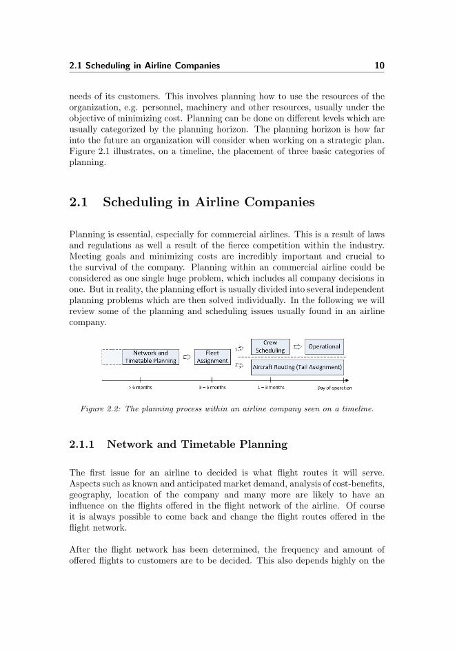
In this chapter we will look at general problems that are related to the BJARP.We will describe how the planning process in a regular airline company usually isperformed and look at the differences compared to the planning in a business jetairline. We will also look at literature on the problems arising in the planningprocess in both regular and Business Jet Airline Companies. We begin thischapter by introducing the concept of planning.
Figure 2.1: The planning horizon. The planning can be categorized as Strategic whichis a long term planning usually performed years before operation. Tactical planningwhich is medium term planning, usually done several to few months before operation.And the Operational planning which is done on a short term basis, days or hours beforeoperation.
Planning is the way an organization defines its strategy or direction. It is of greatimportance for an organization to optimize performance in order to competewith other organizations. The crucial goal for any organization is to meet the
2.1 Scheduling in Airline Companies 10
needs of its customers. This involves planning how to use the resources of theorganization, e.g. personnel, machinery and other resources, usually under theobjective of minimizing cost. Planning can be done on different levels which areusually categorized by the planning horizon. The planning horizon is how farinto the future an organization will consider when working on a strategic plan.Figure 2.1 illustrates, on a timeline, the placement of three basic categories ofplanning.
2.1 Scheduling in Airline Companies
Planning is essential, especially for commercial airlines. This is a result of lawsand regulations as well a result of the fierce competition within the industry.Meeting goals and minimizing costs are incredibly important and crucial tothe survival of the company. Planning within an commercial airline could beconsidered as one single huge problem, which includes all company decisions inone. But in reality, the planning effort is usually divided into several independentplanning problems which are then solved individually. In the following we willreview some of the planning and scheduling issues usually found in an airlinecompany.
Figure 2.2: The planning process within an airline company seen on a timeline.
2.1.1 Network and Timetable Planning
The first issue for an airline to decided is what flight routes it will serve.Aspects such as known and anticipated market demand, analysis of cost-benefits,geography, location of the company and many more are likely to have aninfluence on the flights offered in the flight network of the airline. Of courseit is always possible to come back and change the flight routes offered in theflight network.
After the flight network has been determined, the frequency and amount ofoffered flights to customers are to be decided. This also depends highly on the

2.1 Scheduling in Airline Companies 11
forecasted market demand as well as many other considerations. This phaseresults in a schedule, which usually, but not necessarily is cyclic.
Besides determining which flights to offer customers, how much manpowerneeded and what equipment to purchase are also large planning problems, whichshould be looked at early in the airline planning process.
In the following sections we will briefly describe some of the different types ofplanning.
2.1.2 Fleet Assignment
When the flight schedule is created, flights are to be assigned a specificequipment type, so as to minimize the number of rejected customers (passengerspill) and to maximize profit. The specifications for each equipment type, suchas number of seats and operational costs, and the number of aircraft available foreach type is given. Likewise, a forecasted demand for each flight is known. Giventhis information, the fleet assignment problem is to assign an equipment type toeach flight without using more equipment than available. For more informationon the fleet planning problem, see (Smith and Johnson, 2006) or (Klabjan, 2003),which also provides a mathematical model of the fleet assignment problem. Wewill not present any model of the problem here, as it is not relevant for thisthesis.
2.1.3 Aircraft Routing (Tail Assignment)
Each flight has now been assigned a specific equipment type. The next problemis to assign the specific named aircraft to the flights. This is some times calledtail assignment, given that the tail numbers of each individual aircraft is assigneda flight. The result of this procedure is a sequence of flights or route for eachindividual aircraft. The assignment of aircraft to flights cannot use more thanthe available number of aircraft, and must cover every flight exactly once. Anymaintenance requirements are to be met, likewise are other requirements for theaircraft. The maintenance requirements are often continual and cyclic.
Aircraft routing is performed varying from months before operation up until theday of operation.
Since the aircraft routing problem is based on the solution to the fleet assignmentproblem, these can be considered as separate problems, one for each equipment

2.1 Scheduling in Airline Companies 12
type. The objective is as usually to minimize costs, but this can of course varyfrom company to company.
Since it is difficult to assign a cost to a given aircraft route, the issue is treated insome airline companies as a pure feasibility problem. In (Sandhu and Klabjan,2004) more detailed information is provided about the Aircraft Routing problem.
2.1.4 Crew Scheduling
In the previous problems a timetable for flights and a routing for each individualaircraft were created. The crew scheduling problem consists of preparing aschedule for the staff to be assigned the flights. In the Crew Scheduling problemit is assumed that a given plan of trips exists. The goal is to cover all flights withthe staff needed, while minimizing the operating costs and still complying withrules and regulations. There can be other objectives to take into account, likethe robustness of the scheduling plan. Robustness of a schedule can be describedas the ability to avoid changes in the schedule when disruptions occur. If theairline experiences disruptions that cause delays, it is possible that the schedulecannot be followed depending on the tightness in the plan. If one flight isdelayed, it can cause a snowball effect if there is not incorporated enough bufferin the schedule.
Usually there are requirements for different crew types on every flight. Crewmembers can be based at various crew bases and can have different qualificationsand ranks. The crew can be composed of different types of members/employees,such as captains, first-officers, cabin crew and so forth.
The Crew Scheduling problem is usually divided into two problems: the CrewPairing problem and the Crew Rostering problem (or assignment problem). Thesolution of the crew pairing problem is employed in the crew rostering problem.In the following two sections we will explain the two problems.
Figure 2.3: The Airline Crew Scheduling process.

2.1 Scheduling in Airline Companies 13
2.1.4.1 Crew Pairing
The first part of the Crew Scheduling problem is the Crew Pairing problem. Itconsists of grouping together flights into what is called pairings. An individualpairing consists of a sequence of flights, where the destination airport of a flightin the sequence corresponds to the origin airport of the next flight. Additionally,the origin airport of the first flight and the destination airport of the last flightmust correspond to the same crew base.
In the pairing stage, pairings are not assigned particular crew named members.Each flight should be part of exactly one pairing, so that all flights are coveredexactly once. The pairings are usually created so as to minimize costs, whilesatisfying regulatory rules such as work, rest time and other regulations imposedby company and union policy as well as other authorities within the area. Formore examples of the rules and regulations to comply with in the Crew Pairingproblem, see (Klabjan, 2003).
The Crew Pairing problem can be modeled as a set partitioning model withside constraints. In the following set partitioning model, P denotes the set ofall feasible pairings, F the set of all flights, cp the cost of pairing p ∈ P andyp a binary decision variable that assumes value 1 if pairing p is chosen to be apart of the solution and 0 if not. afp is a parameter that assumes the value 1 ifflight f is in pairing p and 0 otherwise.
min:∑p
cp · yp
st.:∑p∈P
afp · yp = 1 ∀f ∈ F, ∀p ∈ P (2.1)
yp ∈ {0, 1} ∀p ∈ P
The model stated is inspired from (Larsen, 2006).
Side constraints are not shown in the model, but can be used to model forexample equal use of resources and manpower requirements. The equality signin equation (2.1) ensures that all flights are covered exactly once. In some casesit could be preferable to allow a flight to be covered more than once, as thiswould mean that “deadheading” is allowed. “Deadheading” in this case meansthat crew are merely transported on a flight they are not assigned work on.To allow “deadheading”, the equality sign in equation (2.1) can be substitutedwith a greater-or-equal-to sign, which would transform the problem into a setcovering problem. In practice “deadheading” is costly because of the extra crewthat are assigned the flight that is covered more than once, but can sometimesbe beneficial to allow.

2.1 Scheduling in Airline Companies 14
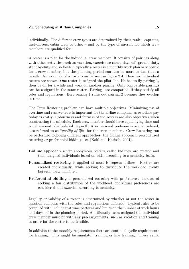
In figure 2.4 it is illustrated how individual flights are distributed into pairings.The flights are the green boxes. The letters on the boxes indicates thegeographical departure airport and destination airport. It is illustrated wherethe flights are located on the timeline. Only compatible flight can be part of thesame pairing. Here flight A→ D and C → B are not compatible as they overlapin time. All flights are part of exactly one pairing. The pairing is constructed insuch away that the pilot finish the pairing in the same airport as the departureairport.
Figure 2.4: The crew scheduling process is illustrated. The boxes are flights where thedeparture and destination are stated in the box. Flights are distributed into pairings.All flights are covered exactly once. Two flights can only be a part of the same pairing ifthey are compatible. Compatible pairings are then assigned rosters. Here two individualrosters are shown.
For further literature on the problem see (Johnson and Gopalakrishnan, 2005),(Barnhart et al., 1998) and (Klabjan, 2003).
2.1.4.2 Crew Rostering
In the next stage, the Rostering stage, the pairings are assigned crew members.The assignment of the found pairings to crew members creates a roster for eachindividual crew member, and should ensure that the crew requirements are metfor each pairing. The problem can be split up and solved for each crew type
2.1 Scheduling in Airline Companies 15
individually. The different crew types are determined by their rank – captains,first-officers, cabin crew or other – and by the type of aircraft for which crewmembers are qualified for.
A roster is a plan for the individual crew member. It consists of pairings alongwith other activities such as vacation, exercise sessions, days-off, ground-duty,standby-duty and so forth. Typically a roster is a monthly work plan or schedulefor a crew member, but the planning period can also be more or less than amonth. An example of a roster can be seen in figure 2.4. Here two individualrosters are shown. One roster is assigned the pilot Joe. He has to fly pairing 1,then be off for a while and work on another pairing. Only compatible pairingscan be assigned in the same roster. Pairings are compatible if they satisfy allrules and regulations. Here pairing 1 rules out pairing 2 because they overlapin time.
The Crew Rostering problem can have multiple objectives. Minimizing use ofovertime and reserve crew is important for the airline company, as overtime paytoday is costly. Robustness and fairness of the rosters are also objectives whenconstructing the schedule. Each crew member should have equal flying time andequal amount of scheduled days-off. Also personal preferences are considered,also referred to as “quality-of-life” for the crew members. Crew Rostering canbe performed following different approaches: the bidline approach, personalizedrostering or preferential bidding, see (Kohl and Karisch, 2004).
Bidline approach where anonymous rosters, called bidlines, are created andthen assigned individuals based on bids, according to a seniority basis.
Personalized rostering is applied at most European airlines. Rosters arecreated individually, while seeking to distribute the workload evenlybetween crew members.
Preferential bidding is personalized rostering with preferences. Instead ofseeking a fair distribution of the workload, individual preferences areconsidered and awarded according to seniority.
Legality or validity of a roster is determined by whether or not the roster inquestion complies with the rules and regulations enforced. Typical rules to becomplied with include rest time patterns and limits on the number of work hoursand days-off in the planning period. Additionally tasks assigned the individualcrew member must fit with any pre-assignments, such as vacation and trainingin order for the roster to be feasible.
In addition to the monthly requirements there are continual cyclic requirementsfor training. This might be simulator training or line training. These cyclic

2.1 Scheduling in Airline Companies 16
requirements have to be respected and can hence effect how the exercise sessionsneed to be placed in the rosters.
The schedule for the planning period consists of all chosen rosters, one for eachcrew member. The problem is modeled as a generalized set partitioning modelfor each crew type. The idea is to generate many possible rosters respecting pre-assignments for each crew member. Then we wish to find a feasible selectionamong these rosters so as all pairings are covered by the required crew and allcrew members are assigned exactly one roster. In the following model, inspiredby (Barnhart et al., 2003), K is the set of crew members of a given type. The setof rosters feasible for crew member k is denoted Rk. P is the set of all pairingsto be covered, and np is the number of the given type that pairing p requires.The cost of assigning roster r to crew member k is specified in cr,k. The costcan depend on the crew member’s salary, home base and other factors. αr,p isa parameter which assumes the value 1 if roster r is included in pairing p and 0otherwise. np is the minimum number of required crew members in pairing p.
min:∑k∈K
∑r∈Rk
cr,k · yr,k
st.:∑k∈K
∑r∈Rk
αr,p · yr,k ≥ np ∀p ∈ P (2.2)
∑r∈Rk
yr,k = 1 (2.3)
yr,k ∈ {0, 1} ∀r ∈ Rk, ∀k ∈ K
In the model yr,k is a binary decision variable which assumes value 1 if roster ris assigned crew member k, and 0 if not.
Equation (2.2) guarantees that all pairings are covered by the selected rosterswith at least the minimum crew requirements. Equation (2.3) ensures thatprecisely one roster is assigned each crew member. Any rules and regulationsinvolving several rosters are not modeled here.
The Crew Rostering problem has been studied for many years and there areplenty of literature on the area. Commonly used solution approaches includeBranch-and-Price, heuristic methods and integer programming.
The characteristics of Crew Rostering problems along with descriptions oftypical rules and regulations are described in (Kohl and Karisch, 2004). Thearticle outlines how a mathematical model of the problem is constructed,applying some examples of vertical rules.
In (Caprara et al., 1998) an instance of the Crew Rostering problem is
2.2 Scheduling in Business Jet Airlines 17
modeled and solved. To solve the problem a heuristic algorithm is designedand implemented. (Fahle et al., 2002) solves the problem using ConstraintProgramming based Column Generation. (Cappanera and Gallo, 2004) presentsa 0 − 1 Multi-Commodity Flow approach to the Crew Rostering problem. Tosolve this model efficiently they go a long way to identify and strengthen differentfamilies of valid inequalities for tightening the formulation.
The problem has been discussed in several other papers including (Teodorovicand Lucic, 1998), (Gamache et al., 1999), (Yunes et al., 2000), (Day and Ryan,1997) and (Medard and Sawhney, 2007).
2.1.5 Aircraft and Crew Recovery
In a perfect world, airline companies could follow what they have planned, andhence minimize operational costs and maximize profit. However when followinga large plan for both aircraft and crew members, it is common for an airlinecompany to experience disruptions, making the plan infeasible. Planners seekto construct all schedules to be as robust as possible, but it is unavoidable thatdisruptions sometimes influence the schedule plan. Disruptions can be causedby unavailable crew or aircraft because of delays or illness. Also a change indemand can occur, which results in broken fleet assignment solution and brokentail assignment solution and hence a broken crew schedule. Other disruptionssuch as congestion and bad weather can cause an aircraft to be grounded forlonger time than the schedule allows. Disruption management is the problem ofdealing with disruptions in a way that minimizes further costs. Other objectivesare to limit the extent of the change necessary and to return to the plannedschedule as soon as possible.
For more and a detailed description of the disruption management issues andapplied strategies for recovery, see (Kohl et al., 2007).
2.2 Scheduling in Business Jet Airlines
Due to the nature of the demand in Business Jet Airlines, most of the planningprocess methods described in section 2.1 for a timetable based airline companyare not applicable in a business jet airline company.
Business Jet Airlines differ from commercial airline companies primarily dueto the fact that no predetermined timetable exists. Customers simply contact

2.2 Scheduling in Business Jet Airlines 18
the company and book a flight up until a few hours in advance. The planningprocess in a business jet airline company is illustrated in figure 2.5. The followingsections are structured similar as for the planning process for a timetable basedairline company in order to clarify the differences in the two processes.
Figure 2.5: The planning process in a Business Jet Airline Company. The“transparency” of the extended planning boxes indicate that planning can be donerepeatedly, due to the dynamic arrival of customer requests.
2.2.1 Network and Timetable Planning
Market analysis to optimize revenue is just as important for a Business JetAirline Company as for a commercial airline company. The decision of howmany aircraft to purchase and which kinds can in a strategic planning problembe determined by the market demand. However we assume that in a business jetairline, demand is not partitioned into demand on different routes, but instead asa demand for fractional shares. For this reason, the network might not be createdbased on the demand for specific flight routes, but more so by the airportspossible to serve. The network will thus consist of all possible combinationsof the airports the aircraft can use. This means that the network, as opposedto a network in a timetable-based airline company, has no stopovers, but is apoint-to-point network.
When a customer requests a flight, the departure time, location and destinationare specified. All requests from customers determine the timetable and the flightnetwork. Hence the flight schedule is neither fixed nor cyclic like for normalairline companies. Since flights can be requested until a few hours in advancethe flight scheduling phase is driven by the flights requested from customers andnot by demand forecasted months in advance (the process is demand-driven).

2.2 Scheduling in Business Jet Airlines 19
2.2.2 Fleet Assignment
In the Fleet Assignment problem for timetable-based airline companies, theobjective is to maximize the profit based on the forecasted demand for eachflight. This is done by assigning a fleet type to each flight. For a BusinessJet Airline Company this process is quite different. In most cases the type ofaircraft assigned a given flight is the type in which the fractional shareholderhas a share. However the planners can alter the aircraft type if it proves moreprofitable. Upgrading the customer to a larger and more comfortable aircraftcan be done with no further expense for the customer, but this potentially hasa cost for the company. A downgrade can also occur according to contractualagreements.
2.2.3 Aircraft Routing
As for the Aircraft Routing problem for a timetable based airline company,the aircraft routing problem for a Business Jet Airline consists of assigningindividual tail numbers to flights. However, as the flights are determinedupon requests of the customer, the flights rarely match in departure locationand destination. Thus, repositioning is necessary. Repositioning means thatthe crew has to fly an empty aircraft to another destination for a customer.Repositioning is rarely needed in regular airline companies given that the routesof aircraft can nearly always be planned ahead. Because the repositioningrepresents a large operational cost for business jet airline companies, minimizingthe repositioning is very desirable.
2.2.4 Crew Scheduling
Crew Scheduling in a Business Jet Airline is quite different from Crew Schedulingfor a timetable-based airline company. Because of the special demands relatedto flights in a business jet airline, Crew Scheduling, like Aircraft Routing, isplanned only a few days or even hours in advance.
Thus, work schedules for crew members cannot be planned and published in theCrew Pairing phase, as is the case for timetable-based airlines. Instead workschedules are published a month or so in advance. These are constructed withouttaking any flights into account and hence there are no geographical aspectsinvolved. The schedules consist of duty periods lasting a specified number ofdays followed by an off-duty period. The work schedules, like generated rosters

2.2 Scheduling in Business Jet Airlines 20
in the crew rostering phase for timetable based airline companies, take pre-assignments such as simulator training into account.
A crew member begins and ends his duty at different locations from day to day.When a crew member begins a duty he has to travel from his crew base to theavailable aircraft to which he has been been assigned. Likewise, when a crewmember ends his duty he travels back to his crew base.
The Crew Scheduling process is often integrated with the aircraft routingproblem due to the fact that it often is assumed that the crew follows oneaircraft, i.e. no crew swaps are performed. However this method imposescrew regulations upon the aircraft. So when creating a pairing, rules regardingminimum overnight rest time and maximum number of flying hours in a dayhave to be respected, and these rules are transferred to the aircraft as well. Insection 2.2.5 we will look further into the related literature and see how thisproblem has been approached in previous work.
2.2.5 Previous Work on the Planning Process in a Busi-ness Jet Airline Company
The literature about scheduling in a Business Jet Airline Company is fairlyrecent and very limited, as the problem has only been studied in OperationsResearch for a relatively short period of time. As we mentioned during themarket analysis in section 1.2 the concept has only existed since 1986 withthe founding of the company NetJets. Major competing Business Jet AirlineCompanies have appear later. In the following we will go through methodsdescribed in the literature for solving various scheduling problems for BusinessJet Airline Companies.
(Keskinocak and Tayur, 1998) is the earliest study found regarding scheduling ina Business Jet Airline Company. They study an aircraft scheduling problem fora single type of aircraft, subject to maintenance requirements and pre-assignedtrips. Multiple fleet and crew related issues are not considered. (Ronen, 2000)studies a combined fleet assignment and aircraft routing problem for charteraircraft with multiple fleet and presents a decision support system tool thatincorporates maintenance activities and crew availability. This tool embodies aset partitioning model. (Martin et al., 2003) describes another decision supportsystem tool that handles all aspects of the planning for a fractional ownershipairline company. This tool can create an optimal aircraft routing schedule basedon owner demand, taking feasibility rules into account while minimizing costs.An integer programming model for a aircraft routing problem is presented whichincludes multiple aircraft types and crew constraints.
2.3 Related Problems 21
(Hicks et al., 2005) present an optimization system developed for BombardierFlexjet, which is a Business Jet Airline Company. The optimization systemdivides the planning process into three phases:
1. Monthly crew rosters are created based on pre-assignments and estimateddemand.
2. Integrated flight scheduling, fleet assignment, aircraft routing and crewscheduling.
3. Assignment of crew members to duties on specific aircraft, performed everyday before operation.
The article describes how Bombardier Flexjet has improved their operations.The system applies Column Generation to simultaneously maximize the useof aircraft, crew and facilities. The outcome is personalized crew schedules aswell as aircraft routings. (Yao et al., 2008) propose a set partitioning modelfor the combined aircraft routing and crew scheduling problem. The modelis solved using a Column Generation approach. It is discussed how severaloperational and tactical planning issues affect the profitability in a BJAC. In(Yang et al., 2008) mathematical models, exact and heuristic solution methodsare presented for aircraft routing. A network flow model is developed thatcreates crew feasible schedules for the aircraft. A heuristic for the combinedaircraft and crew scheduling problem is also described.
In (Espinoza et al., 2008a) and (Espinoza et al., 2008b) an aircraft routingproblem for the “dial-a-flight” concept is discussed. An integer multi-commoditynetwork flow model with side constraints is presented. The problem is solvedusing a parallel large neighborhood local search scheme in (Espinoza et al.,2008b).
To our knowledge, there are no relevant papers on the first phase of thecrew scheduling, in which the rosters are created without the use of generatedpairings.
2.3 Related Problems
In this section we will introduce some classes of problems that are related to orhave similar characteristics as planning problems for Business Jet Airlines.

2.3 Related Problems 22
2.3.1 Personnel Scheduling
Personnel scheduling deals with the construction of work timetables for per-sonnel in an organization, making it possible for the organization to meetthe demand for the service the company provides to its customers. Thereare many well-studied problems within personnel planning and scheduling, inmanufacturing as well as in services. The airline business, and hence ourproblem, is categorized in the service area. Therefore we will concentrate onproblems inherent in this area as well.
Depending on the characteristics of the problem, several issues need to beconsidered when developing schedules for staff members. The first step for acompany is to determine the staff requirements for company services neededin order to fulfill the demand. The demand may vary over time during theplanning horizon and can be uncertain for the Business Jet Airline case. Thedemand can either be known or estimated. If the demand is estimated, this isan important part of the planning process, as it will have a large influence onthe ability to meet the real demand in the end.
Workforce planning is the process of determining the level of required staff.This problem is a strategic planning problem. When dealing with uncertaindemand, as is often seen in service areas, this stage of the planning process ishighly essential. If the level of staff cannot cover the daily staff requirements,the demand cannot be met.
The scheduling process of a problem also depends on the characteristics of thedemand. In some companies, shift scheduling is applied. Shift scheduling is theprocess of determining shifts to be worked from a large pool of possibilities andalso within these shifts an assignment of the number of staff required for eachshift. In Crew Pairing, the scheduling is performed using task-based demand,where the main task is to select, from a large pool of possibilities the best set ofpairings (shifts) in order to cover all tasks. If the demand is already shift basedthis process of the planning is of course unnecessary.
The outline of the rostering process depends on the building blocks used.Building blocks in the crew rostering problem in a timetable-based airlinecompany are usually training sessions, pairings and days-off periods. In the caseof dealing with Crew Pairing the rostering process is called Crew Rostering.When dealing with uncertain, demand the rostering process is sometimesreferred to as Tour Scheduling. Tour Scheduling is a combination of ShiftScheduling and Days-off Scheduling. Days-off Scheduling is the problem ofdetermining the distribution of rest days, between the work days. The tourscheduling problem involves assigning days-off, as well as assigning shifts to the

2.3 Related Problems 23
staff on their work days and is a tactical planning problem. In the rosteringprocess, the assignment of rosters can either be done during the process orafterward, depending on the characteristics of the given problem.
Task assignment may be necessary if different tasks need to be performed duringeach shift. Tasks may have requirements for particular staff skills. This feature iswhat is seen in the crew scheduling process for Business Jet Airline Companies.Schedules are created approximately a month in advance and the crew membersare then assigned tasks, that is pairings, days or even hours before operation.The tasks require different staff skills, namely those of a captain and a first-officer.
These personnel scheduling problems have their application in many other areas.Application areas that are relevant for our problem and that include similarelements are mentioned and briefly described in the overview table 2.1.
For further literature on general personnel scheduling and methods used forsolving the class of problems, an overview is given in (Ernst et al., 2004).
2.3.2 Transportation on Demand
Something thas is common to Transportation on Demand problems is that usersrequest transportation from pickup point to destination point. The type oftransportation can be of goods or passengers. The problems can be either staticor dynamic. Typically the objective in such transportation problems is oftena mix of several. It is desirable to maximize the number of requests served.In the case of the Business Jet Airline, serving all customers is a requirement.Other objectives are to minimize operational costs as well as to reduce userinconvenience, that is maximizing goodwill. These objectives can be conflictingand a balance between them has to be accomplished.
Time windows usually exist in Transportation on Demand problems. A timewindow is defined by the first and last time where a service can be performed. Insome problems time windows are hard, defining that they cannot be exceeded orsoft where they can be violated at a certain cost. Especially when transportingpeople, narrow (and usually hard) time windows are in force.
In the Vehicle Routing Problem with Pickup and Delivery (VRPPD) a givennumber of vehicles or commodities are used. There are requests to be met andeach request has a pickup point and a delivery point associated with it. If theserequests also have a given time window in which it has to be performed, theproblem is called the Vehicle Routing Problem with Pickup and Delivery with

2.3 Related Problems 24
Application area Description LiteratureTransportation systems Demand generated from exist-
ing timetables, geographicalaspects involved. Seen inrailway, airline, buses andmass transit.
(Ernst et al.,2004), (Ernstet al., 2001),(Sarin andAggarwal,2001)
Call centers Tasks not known a priorybecause of estimated demand.Shortage and surplus are ex-perienced according to actualdemand. Seen at companyhotlines, subscription centers,receptions and booking of-fices.
(Atlasonet al., 2004),(Hendersonand Berry,1976)
Health care systems “The nurse schedulingproblem”. Rosters for nurses.Rosters must comply withmany rules and regulations.Seen at hospitals, nursinghomes and other carefacilities.
(Cheanget al., 2003),(Berradaet al., 1996),(Bellantiet al., 2004),(Beaulieuet al., 2000),(Berlien andDemeule-meester,2006)
Table 2.1: Descriptions and literature references of application areas for personnelscheduling problems.
Time Windows (VRPPDTW). The number of available vehicles is also given,each of these with a capacity limit. Also there is a limit on the duration of aplanned route for each vehicle. Each pickup and delivery point has a serviceand load time. A request has a cost and a travel time connected to it. Theproblem is then to find the optimal routes for the vehicles in such a way thatall requests are met and costs are minimized. This is done while respecting thetime windows and capacity constraints.
If a full truckload is assumed, the VRPPDTW resembles the aircraft routingproblem for both timetable-based airline companies and even more so forBusiness Jet Airline Companies. “Full truckload” means that the capacity ofthe vehicle is exactly the capacity of the goods on each request, so that only one

2.3 Related Problems 25
request can be served by one vehicle at a time. In the Aircraft Routing problemfor business jet airline companies, flights are requests and with each request atime window is given as well as a pickup and drop off point. The number ofavailable vehicles is the number of available aircraft within a certain fleet type.When the assumption is made that the crew members follow the aircraft, thefull truckload VRPPDTW can be compared to the integrated Aircraft Routingand Crew Scheduling process in a business jet airline company. Some crewconstraints can be formulated as constraints on the maximum allowed durationof a route.
For further information on the Full Truckload Vehicle Routing Problem withpickup and delivery, see (Yang et al., 2004). For a broader view of transportationon demand see (Cordeau et al., 2003).
We have now had a closer look into planning problems that have characteristicsin similar with the Business Jet Airline Rostering Problem. We have describedthe planning process of a business jet airline company and compared this tothe planning process of a time table based airline company. The problem hasbeen placed within the Business Jet Airline planning process. In the followingchapter we will further examine the details of specific the Business Jet AirlineRostering Problem, which is the basis of this thesis.

Chapter 3
The Case: Rostering for aBusiness Jet Airline Company
The topic of this thesis, a case of the Business Jet Airline Rostering Problem(BJARP) was briefly described in section 1.3. In this chapter we will elaborateon the specific problem, including the specific rules and the goals of the problem.The chapter is structured in the following way. Initially we will provide amore detailed description of the problem and then move on to the potentialobjectives when solving the problem. Hereafter we will examine rules present inthe problem. The rules will be divided into horizontal and vertical rule types.A definition of these classification types will also be provided.
This case study Business Jet Airline Rostering Problem (BJARP) is an realproblem stemming from a Business Jet Airline Company. However we have nothad the opportunity to work directly with this company. We have worked onthe problem together with Jeppesen Systems who has provided information onproblem characteristics, rules and potential goals of the problem.
3.1 The Business Jet Airline Rostering Problem 27
3.1 The Business Jet Airline Rostering Problem
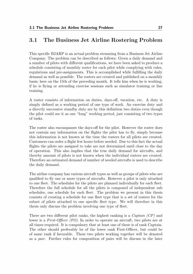
This specific BJARP is an actual problem stemming from a Business Jet AirlineCompany. The problem can be described as follows: Given a daily demand anda number of pilots with different qualifications, we have been asked to produce aschedule consisting of monthly roster for each pilot while complying with rules,regulations and pre-assignments. This is accomplished while fulfilling the dailydemand as well as possible. The rosters are created and published on a monthlybasis; here on the 15th of the preceding month. It tells him when he is working,if he is flying or attending exercise sessions such as simulator training or linetraining.
A roster consists of information on duties, days-off, vacation, etc. A duty issimply defined as a working period of one type of work. An exercise duty anda directly successive standby duty are by this definition two duties even thoughthe pilot could see it as one “long” working period, just consisting of two typesof tasks.
The roster also encompasses the days-off for the pilot. However the roster doesnot contain any information on the flights the pilot has to fly, simply becausethis information is not known at the time the rosters for all pilots are created.Customers can order a flight few hours before needed. Due to this fact the actualflights the pilots are assigned to take are not determined until close to the dayof operation. This also implies that the true daily demand for aircrafts, andthereby amount of pilots is not known when the individual rosters are created.Therefore an estimated demand of number of needed aircrafts is used to describethe daily demand.
The airline company has various aircraft types as well as groups of pilots who arequalified to fly one or more types of aircrafts. However a pilot is only attachedto one fleet. The schedules for the pilots are planned individually for each fleet.Therefore the full schedule for all the pilots is composed of independent subschedules, one schedule for each fleet. The problem we present in this thesisconsists of creating a schedule for one fleet type that is a set of rosters for thesubset of pilots attached to one specific fleet type. We will therefore in thisthesis only discuss the problem involving one type of fleet.
There are two different pilot ranks, the highest ranking is a Captain (CP) andlower is a First-Officer (FO). In order to operate an aircraft, two pilots are atall times required. It is compulsory that at least one of these is of rank Captain.The other should preferably be of the lower rank First-Officer, but could beof same rank if favorable. These two pilots working together will be denotedas a pair. Further rules for composition of pairs will be discuss in the later
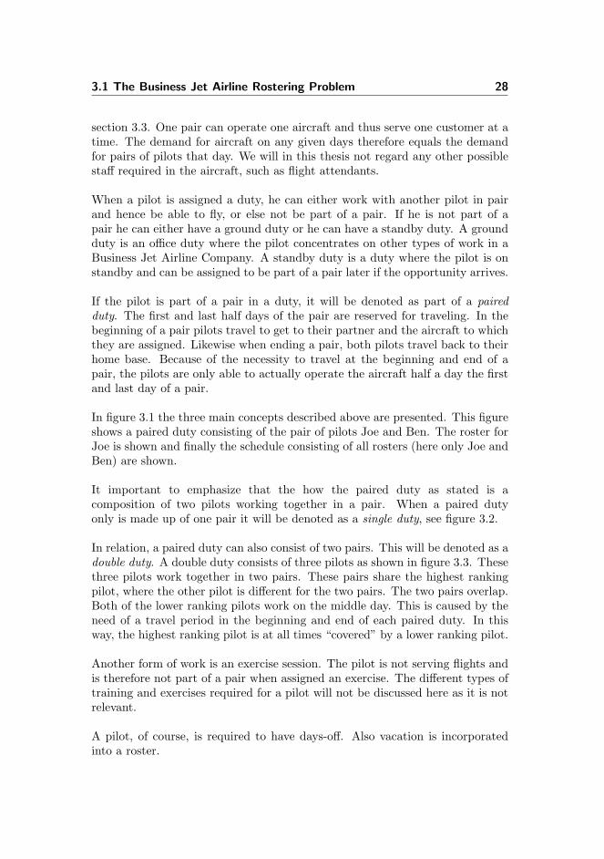
3.1 The Business Jet Airline Rostering Problem 28
section 3.3. One pair can operate one aircraft and thus serve one customer at atime. The demand for aircraft on any given days therefore equals the demandfor pairs of pilots that day. We will in this thesis not regard any other possiblestaff required in the aircraft, such as flight attendants.
When a pilot is assigned a duty, he can either work with another pilot in pairand hence be able to fly, or else not be part of a pair. If he is not part of apair he can either have a ground duty or he can have a standby duty. A groundduty is an office duty where the pilot concentrates on other types of work in aBusiness Jet Airline Company. A standby duty is a duty where the pilot is onstandby and can be assigned to be part of a pair later if the opportunity arrives.
If the pilot is part of a pair in a duty, it will be denoted as part of a pairedduty. The first and last half days of the pair are reserved for traveling. In thebeginning of a pair pilots travel to get to their partner and the aircraft to whichthey are assigned. Likewise when ending a pair, both pilots travel back to theirhome base. Because of the necessity to travel at the beginning and end of apair, the pilots are only able to actually operate the aircraft half a day the firstand last day of a pair.
In figure 3.1 the three main concepts described above are presented. This figureshows a paired duty consisting of the pair of pilots Joe and Ben. The roster forJoe is shown and finally the schedule consisting of all rosters (here only Joe andBen) are shown.
It important to emphasize that the how the paired duty as stated is acomposition of two pilots working together in a pair. When a paired dutyonly is made up of one pair it will be denoted as a single duty, see figure 3.2.
In relation, a paired duty can also consist of two pairs. This will be denoted as adouble duty. A double duty consists of three pilots as shown in figure 3.3. Thesethree pilots work together in two pairs. These pairs share the highest rankingpilot, where the other pilot is different for the two pairs. The two pairs overlap.Both of the lower ranking pilots work on the middle day. This is caused by theneed of a travel period in the beginning and end of each paired duty. In thisway, the highest ranking pilot is at all times “covered” by a lower ranking pilot.
Another form of work is an exercise session. The pilot is not serving flights andis therefore not part of a pair when assigned an exercise. The different types oftraining and exercises required for a pilot will not be discussed here as it is notrelevant.
A pilot, of course, is required to have days-off. Also vacation is incorporatedinto a roster.

3.1 The Business Jet Airline Rostering Problem 29
Figure 3.1: A paired duty, where Joe (CP = Captain) is paired with co-pilot Ben (FO= First-Officer). A roster for Joe, consisting of his paired duty with Ben on days 2-5and EXC (exercise session) on days 11-14. A schedule consisting of two rosters, theone for Joe repeated and for Ben his paired duty with Joe on days 2-5, SBY (standbyduty) on days 6-8 and VAC (vacation) on 12-15. OFF denotes Day Off.
Figure 3.2: A single duty - a paired duty made up of one pair from figure 3.1, withboth pilots in the pair, Joe (CP) and Ben (FO). This will be defined as a single duty.

3.2 Objectives of Rostering 30
Figure 3.3: A double duty - a paired duty made up of two pairs. The first pair (Joeand Ben) are as in figure 3.2, but as it is put together with another pair (Joe and Eva)it becomes a double duty. Observe how the highest ranking pilots (Joe) is “covered”through his entire duty by lower ranking pilots (Ben and Eva).
All the different types of events can be pre-assigned. This means that whenconstructing the individual roster, there are events that are already plannedand have to be respected. All other events have to be planned to fit with thepre-assigned ones. Here being off-duty is also regarded as an event. Vacationand exercise sessions are almost always pre-assigned.
Pilots can request for specific days-off, but these requests are not required to begranted.
Certain rules are to be followed for a schedule to be feasible. These rules arestated in the following section 3.3. The objectives present when creating aschedule are discussed in the following section.
3.2 Objectives of Rostering
What are the characteristics of a good solution to a specific problem? This canbe a difficult question to answer, and may depend on who is asked. Due to thefact that we have had no direct contact to the Business Jet Airline Company,i.e. the owner of the problem, no specific goals has been uncovered. Insteadwe have discussed with Jeppesen Systems which characteristics are desirablein a solution. The discussion leaves us with the following characteristics of apotentially good solution:
Obj 1 Maximize the number of paired tour days assigned in the planningperiod, without any regard to daily demand.
Obj 2 Meet demand given by estimated crew requirements.

3.2 Objectives of Rostering 31
Obj 3 Meet requirements as well as possible, while minimizing the largestdeviation (avoid large peaks).
All objectives are under the assumption that all rules and pre-assignments arerespected.
The objective [Obj 1] is to maximize the number of paired tour days in theplanning period. A paired tour day is defined as follows: The number of pairedtour days on one day is the number of pairs of pilots at work on that specificday. The total number of paired tour days in the entire planning period is thesum over the number of paired tour days for each day in the planning period.
When counting the number of paired tour days in a paired duty, the numberof days the pilots actually are able to operate the aircraft are summed. Thehalf days in the beginning and end of the paired duty used for traveling are notincluded. Figure 3.4 shows how the number of paired tour days are counted foreach day in a small problem. It shows how two different paired duties placedwith the ones last day as the same day as the others first can “cover” this daywith regards to paired tour days.
Figure 3.4: How to count the number of paired tour days per day: Count the numberof pairs of pilots able to operate an aircraft, e.g. the half days assigned for traveling(TR) do not count as paired tour days. For example day 2 has 1
2paired tour days due
to the traveling. Day 5 has 1 paired tour day, each pair contributes with a 12
due totheir traveling.
It is desirable to meet the crew requirements for each day [Obj 2], in order tosatisfy demand. However this is not always possible. If the crew requirementscannot be met on all days, it is more desirable to have many days that almostsatisfy the requirements and some that do, as opposed to having many daysthat do satisfy the requirements and a few days that are far from the desired

3.3 Rules and Regulations 32
number of pairs of pilots. This is stated in objective [Obj 3].
How the objectives are prioritized is unknown, however it has been implied thatmaximizing the number of paired tour days is desirable.
3.3 Rules and Regulations
In this section we will introduce classifications of different rule types. Theclassification is inspired by (Kohl and Karisch, 2004). Furthermore we willdescribe the specific rules of the problem and categorize these according to theclassifications introduced.
Rules are divided in two categories: “Horizontal rules” and “Vertical rules”.
A horizontal rule is characterized by the fact that it only concerns one rosterat a time. A rule that is classified as horizontal is the required length of anoff-duty period. This rule applies for all pilots, but concerns individual rosters.
A vertical rule involves more than one roster and hence several crew members.Typically a rule concerns a subset of rosters, but can involve the whole schedule.An example of a vertical rule could be regarding qualifications, i.e. differentcrew qualifications that are needed to operate an aircraft. This rule involvescombinations of pilots and hence more than one roster.
In the following, all specific rules and regulations concerning the Business JetAirline Rostering Problem are described.
3.3.1 Specific Rules in the Case
This section will describe the various rules and regulations imposed by differentfactors. These can be divided into different types corresponding to theclassifications. There are rules regarding individual duty periods and days-off periods for a single pilot, i.e. horizontal rules, and rules regarding teams ofpilots which are the vertical rules.
3.3.1.1 Rules on Single Rosters, Horizontal Rules
The following rules state the rules concerning the individual rosters.
3.3 Rules and Regulations 33
R1 Minimum consecutive days-off (buffer), woff = 5.
R2 Minimum consecutive working days, wmin = 3.
R3 Maximum consecutive working days, wmax = 6.
R4 Minimum consecutive working days of same event, wmin = 3.
R5 Maximum working days in a month, wmonth = 18.
R6 Maximum working days in a quarter, wquarter = 50.
R7 A paired duty must begin and end with half a travel day.
R8 Standby day blocks of lengths {1, . . . , wmin−1} can be assigned in a workingperiod before or/and after the paired tour days. Standby day blocks oflengths {wmin, . . . , wmax} can be assigned as individual working periods ortogether with paired tour days as long as the full length of the consecutiveworking days does not exceed wmax.
The rule [R4] is required due to the fact that one consecutive working period canconsist of several events. While the entire working period has requirement onmaximum and minimum length, the individual event within have a requirementon minimum length. This ensures that a paired duty as part of a working periodof several events, will have the minimum length of wmin.
When applying rules [R5] and [R6], there are special guidelines for counting thenumber of working days over a period. A duty is considered as work regardlessof whether the pilot is part of a pair or not. The travel periods in the beginningand end of a duty and are also counted. All training is considered as work aswell. Vacation is partly considered as work. When a pilot is on vacation, theweekdays count as work and the weekends do not. This means that if a pilothas three weeks of vacation, that is twenty one days, only fifteen of these daysare included when counting the number of working days. With regard to rule[R6], if the planning period is less than a quarter data for each pilot regardingnumber of work days the last quarter is given.
In table 3.1 an overview of the different events is presented. For each event it isspecified which rules apply as well as if the event are included as work and henceincluded when counting the number of work days in a month or quarter. Eventsthat are pre-assigned do not necessarily follow all rules stated. For examplea pilot could be scheduled to an exercise session lasting more than wmax daysor be scheduled to have two exercise periods closer than woff days apart. Apre-assigned event is registered as work if the event normally would be countedas such.
We now move on to describe the rules that involve more than one roster.

3.4 Briefly on Jeppesen Systems Solution Approach 34
Event [R1] [R2] [R3] [R4] [R5] [R6] [R7] [R8]Duty x x x x x xGround duty x x x x xStandby duty x x x x x xExercise x x x x xVacation x x (x) (x)Days-off x
Table 3.1: Overview of which rules apply for the different events. [R1]: Min consecutivedays-off, [R2]: Min duty length, [R3]: Max duty length, [R4]: Min length of event type,[R5]: Max work month, [R6]: Max work quarter, [R7]: Travel in duty, [R8]: Standbydays.
3.3.1.2 Regulations Between Pairs of Pilots, Vertical Rules
A list of the rules in the problem that involves two or more rosters is providedbelow.
R9 A pair of pilots consists of either a Captain and First-officer or two Captains.When two Captains are paired up, the most senior must act as Captainand the other as First-officer. Two low-timer pilots cannot constitute apair.
R10 Maximum consecutive duties in the same pair, wsame = 2.
Rule [R9] defines which pairs of pilots are legal in a paired duty. Rule [R10]state that there is a limit on how many consecutive times a pilot can work withanother pilot.
This concludes the rules in the Business Jet Airline Rostering Problem. In thefollowing section we will shortly describe the solution approach used by JeppesenSystems to solve this problem.
3.4 Briefly on Jeppesen Systems Solution Ap-proach
The BJAC behind the case in this thesis is a customer of Jeppesen Systems.They have designed a special rostering system for solving this customersproblems. We do not have detailed knowledge regarding the solution approach

3.4 Briefly on Jeppesen Systems Solution Approach 35
Jeppesen Systems has applied for solving this problem. However in order tojustify the methods we have chosen to implement we will briefly give an overviewof the information we have been given regarding the solution approach appliedby Jeppesen Systems.
Jeppesen Systems applies a Column Generation solution approach where acolumn corresponds to a single roster for a pilot. The columns do not takepaired duties into account. The assignment of pairs are done afterward. Manylegal rosters for all pilots are generated. When solving the problem of assigningexactly one roster to each pilot, it is taken into account that all duties ofthe pilots must be paired. The solver used then optimizes the problem whileensuring that all duties in the assigned rosters are being paired.
By not assigning the pilots in pairs to begin with the amount of possible rostersare less than if all possible pairs in a duty were considered.
The problem which is the work of this thesis have now been stated. In the nextchapter we will address some general modeling issues of the problem. Furthermore we will discuss some assumptions we make regarding the interpretationof the problem. We will additionally look at how to express the objectivesdiscussed in section 3.2 mathematically.
Chapter 4
Modeling Issues, Objectives,Analysis and Bounds
This chapter consists of the following parts: Initially we will give a discussionof some general assumptions and choices we will make in order to narrow downthe problem at hand which was defined in chapter 3. Hereafter we will lookinto some general modeling issues that are in common to the different methodsof modeling the problem. Next we present bounds and data specifications, andfinally give a short description of the computational environment.
4.1 Current Planning Approach
We do not have many details on how the schedules are created today in theairline company. However we do know that all planning is done manuallywith use of spreadsheets. The planning is done in different stages. Exercisesessions, vacation and special days-off are planned ahead of the creation of theschedule. Pre-assigned paired duties usually stems from the schedule of theprevious month.
With real data we have observed that the rules mentioned in section 3.3 are notalways 100% respected. This can be caused by the planning being done manually

4.2 Assumptions and Choices 37
with inevitable mistakes and errors. In reality rules can be circumvented,especially if the pay off is great.
4.2 Assumptions and Choices
Throughout the thesis we will only look into modeling approaches that includepairing up the pilots from the start. We have chosen to do so because weare interested in exploring other modeling options than the approach JeppesenSystems have applied. We will therefore not discuss alternative methods thatdo not consider pairs of pilots as part of a model.
In order to be able to make correct assumptions and choices we will have tointroduce the following sets. These define the days and time periods that areinvolved in a schedule. Let ndays be the number of days in the schedule, andntp be the number of time periods in each day. The specific problem defines twotime periods, “am” and “pm”. Therefore we will generally refer to these.
J Days in work plan, {1, 2, . . . , ndays}T Time periods per day, {am,pm}
A time unit is defined as one time period within a day. For example in a monthlyschedule a time unit could be day 3 “am”.
4.2.1 Determining the Planning Horizon
We will determine the exact definition of our planning horizon given the planninghorizon from the problem definition. The least required horizon to plan for isthe month of work that must be published to the pilots beforehand. Thereforethis discussion is whether or not planning should take place in a horizon furtherout in the future and if so, how far in the future.
The work plan for the previous month is at the planning stage for the currentmonth considered to be “locked”, that is, no planning is possible before thefirst day of the planning month. This is of course because the previous monthsalready have been planned for. Oppositely, in the other end, the subsequentmonth(s) are not considered to be “locked” and could be included in the planninghorizon. However following from the month-to-month planning, the succeedingmonths are to be planned iteratively over time.
Following that the previous months have been “locked”, the earliest day to place

4.2 Assumptions and Choices 38
a day of a duty within the planning horizon is on the first day of the month.Considering that the initial time period (am) of a duty consists of a TR-segment(Travel), the first time period to actually be able to plan for a paired duty tomeet demand is the second time period (pm) of day one in the month.
Figure 4.1: Different options for the planning horizon for January. The highest ofthe blue lines indicate the shortest possible horizon; this is the month of January andno further days. The following lines below show other possible horizons, where the redindicates the planning horizon we have chosen to use. Note that the initial time periodof each month cannot be planned given that it has already been planned by the planningof the previous month.
To conclude, the choice of our planning horizon is a matter of balancing outtwo conflicting aims. Seen from the perspective of the month to be planneda planning horizon as far out in the future after the month is favorable. Onthe other hand, the higher the extent of planning from the previous month“stretched” into the month to be planned, the less leeway remains for planning.Of course a way of getting around this would be to plan as far out into thefuture as possible, following the more-information-is-better-idea, and then aftersolving the problem removing all duties after a certain day in the subsequentmonth. The planning horizon we choose in this thesis to plan further out in thefuture that the month itself is the maximum duty length for duties starting onthe last day of the month.
In other words, we define our planning horizon J = {jbegin, jbegin + 1, . . . , jend}where jbegin = 1 and jend = ndaysinmonth + wmax − 1. Both jbegin, jend ∈ J .
J Days in counted planning period, {jbegin, jbegin + 1, . . . , jend}
4.2.2 Determining Limits on Quarters
Considering the rules and regulations regarding the maximal amount of work ina quarter (wquarter) arise two options for how this rule is regarded. Eitherthe quarters are looked upon as a running quarters or as regular calendarquarters. The big difference between these two ways is the selection of the

4.2 Assumptions and Choices 39
month that will be bound by the quarter-rule. With regular calendar quarters,planning in any of the third months in each calendar quarter, eg. March, June,September and December, will possibly be restrained by the planning in theprevious two months. The first and with very high likelihood the second monthof each quarter will not be restrained by the quarterly maximum working rule.Oppositely, with running quarters, the planning will for good and bad alwaysbe restrained by the two preceding months. Figure 4.2 gives an illustration ofthese two planning options.
In this thesis we choose to use running quarters. This means that we do notdifferentiate between the months. If we were to plan using regular quartersevery first month in the quarter would have no quarterly working limits. Wewould then have to consider the two upcoming months, so that the first planningmonth in the quarter would not restrict the next two months too much. If usingregular quarters the last month in a quarter could be highly restricted due tothe work planned in the two first months of a quarter. Because of this we chooseto have equally hard restrictions on all months of the year.
Figure 4.2: The two ways of considering quarter-wise planning, either as regularcalendar quarters or as running quarters. Running quarters requires equal informationregardless of the current planning month. The information needed when applyingcalender quarters vary with the time location of the different months.
4.3 Objectives 40
4.2.3 Rules and Features Included in the Models
The events can be divided into two groups, events that are planned more than amonth ahead (pre-assignments) and event types that are planned when creatingthe complete schedule for the pilots. We will focus our work on creating theschedule for the pilots and hence not concentrate on pre-assignments. Eventsthat are planned in the monthly generation of the schedule are paired dutiesand standby duties.
In this work we will focus on how to plan paired duties, which are the only dutytype where the pilots are assigned to operate the aircraft. Hence the pairedduties are the only duty type that can contribute to the satisfactory of thedemand for flights. We will not schedule standby duties for the pilots, as wewill focus on the satisfactory of the given demand.
The rules in the problem were stated in section 3.3. When modeling the problemwe will not model rule [R10] regarding consecutive working partners in any ofthe presented solution methods. Because of the large amount of possible pairsof pilots, as we will see later in this section, the likelihood of more than twoconsecutive duties with the same pilot is not very large. This however canoccur. We have chosen to avoid this by performing a feasibility check on anygenerated solution. If the solution do not satisfy rule [R10] it will be disregardedand a new solution will be generated.
4.3 Objectives
In this section we investigate how to achieve the goals mentioned in chapter 3through the use of various objective functions. For each objective and objectivefunction, we will present the pros and cons with regards to modeling issues andfulfillment of goals. Any choice of objective function will not be mentioned here,but rather this chapter is an assessment of the advantages and disadvantages ofdifferent objective functions.
Note that all rules and regulations which are mentioned in section 3.3, will beassumed to be respected throughout this chapter. That is, any of the introducedobjectives in this chapter will of course have an influence on solution quality,but will not influence on solution legality. We will in later chapters examinehow legality according to rules and regulations is ensured in different ways ofmodeling the problem at hand.
4.3 Objectives 41
Before presenting the objective functions we will give a brief introduction to ageneric way of modeling the problem. For simplicity, we will not consider dutiesto be paired in this chapter. In other words modeling issues ensuring that apair in a paired duty consists of two (single duty) or more pilots (double duty)working together in agreement will be disregarded. Omitting this part of theproblem leaves us with a different problem where the only decision to make ison which days each pilot works.
4.3.1 Objective Functions
We will give a brief introduction to a generic way of modeling the problem.The problem can be considered as multiple interconnected decisions of whichpilots work on which days. This is the direct equivalent to deciding whethereach pilot works on each day in each time period or not. In other words theproblem consists of a binary decision variable for each pilot, each day and eachtime period. If we define sets P denoting all pilots, J days and T time periods,we can introduce the variables xp,j,t.
xp,j,t :{
1 if pilot p works on day j, time period t0 otherwise
Meeting demand is part of several of the objective functions that will bementioned. The xp,j,t-variables are also used for registering the fulfillment ofdemand. From section 2.1.4 especially the set partitioning and set coveringmodels can be used for this purpose. These are regularly formulated as follows.Demand on day d and time period t will be denoted demd,t.
Set covering:∑p∈P
xp,j,t ≥ demj,t∀j ∈ J, t ∈ T (4.1a)
Set partitioning:∑p∈P
xp,j,t = demj,t∀j ∈ J, t ∈ T (4.1b)
Both formulations (4.1a) and (4.1b) have a major drawback when meetingdemand is not possible. In this case the problem will be considered infeasible.However this depends on how a duty actually is defined. If “dummy” duties withcorresponding penalties for selection are introduced, the problem can again befeasible, even though demand is not actually met. A way of solving these typesof problems where demand potentially cannot be met is by introducing surplusand shortage variables for each “unit” where demand must be met.
s+j,t, s
−j,t : ≥ 0, surplus (+) or shortage (−) on day j, time t (4.2)

4.3 Objectives 42
Introducing these variables into the set partitioning formulation from (4.1b)renders the following useful formulation, which still is a set partitioningformulation, with slack variables. This approach is inspired by (Alfares, 2004)and others. ∑
p∈Pxp,j,t − s+
j,t + s−j,t = demj,t ∀j ∈ J, t ∈ T (4.3)
The formulation (4.3) ensures that whenever the sum of working pilots on a givenday and time period is less than demand, the shortage variable s−j,t compensatesby assuming a value corresponding to the difference between demand and thesum of working pilots. This works in the exact same way for surplus where s+
j,t
compensates and assumes the surplus as its value. It is very important to notethat this constraint could leave the problem unbounded if the surplus or theshortage variables are not concurrently constrained or penalized. Otherwise,both variables can simply assume values “compensating” for each other andthus be unrestricted variables.
Obviously this “trick” with the slack variables s+j,t and s−j,t comes at the cost
of extra variables - one surplus and one shortage variable per day and timeperiod. However the introduction of these variables opens up for many differentconstraint and objective function modeling possibilities.
The following sections will introduce and comment on various objectivefunctions. Several of these objective functions will attempt to minimize thenegative deviation from demand in one formulation or another. Without lossof generality, the word negative can be exchanged with positive throughout thischapter without breaking the formulations and perhaps changing the sense frommaximize to minimize or vice versa.
4.3.1.1 Paired Tour Days (PTD)
This objective function has the goal of maximizing the sum of paired tour days.In other words, the goal is to maximize the sum of working days that contributeto serving customers. It does not use the surplus and slack variables as in(4.3), which therefore are not included in the model along with their relatedconstraints. In its basic form, this objective function can be modeled quiteeasily as follows.
max.:∑
p∈P,j∈J,t∈Txp,j,t
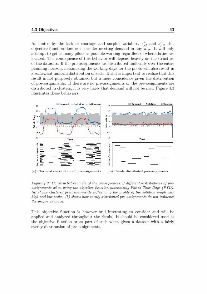
4.3 Objectives 43
As hinted by the lack of shortage and surplus variables, s+j,t and s−j,t, this
objective function does not consider meeting demand in any way. It will onlyattempt to get as many pilots as possible working regardless of where duties arelocated. The consequence of this behavior will depend heavily on the structureof the datasets. If the pre-assignments are distributed uniformly over the entireplanning horizon, maximizing the working days for the pilots will also result ina somewhat uniform distribution of such. But it is important to realize that thisresult is not purposely obtained but a mere coincidence given the distributionof pre-assignments. If there are no pre-assignments or the pre-assignments aredistributed in clusters, it is very likely that demand will not be met. Figure 4.3illustrates these behaviors.
(a) Clustered distribution of pre-assignments. (b) Evenly distributed pre-assignments.
Figure 4.3: Constructed example of the consequences of different distributions of pre-assignments when using the objective function maximizing Paired Tour Days (PTD).(a) shows clustered pre-assignments influencing the profile of the solution graph withhigh and low peaks. (b) shows how evenly distributed pre-assignments do not influencethe profile as much.
This objective function is however still interesting to consider and will beapplied and analyzed throughout the thesis. It should be considered used asthe objective function or as part of such when given a dataset with a fairlyevenly distribution of pre-assignments.

4.3 Objectives 44
4.3.1.2 Sum of Negative Deviation (SoND)
This objective function has the goal of minimizing the sum of negative deviationfrom demand, this is the sum of the shortage variables s−j,t.
min.:∑
j∈J,t∈Ts−j,t
This objective function is different from the PTD in that it considers demandwhen attempting to minimize the negative deviation from the demand. Thereis no gain in assigning more pilots to work in what is necessary for meetingdemand.
However this objective function shares a disadvantage with the PTD. It is a sumoperation, so no consideration is taken with regards to the distribution of thenegative deviation. For example, as a consequence of this, the objective value ofa solution with an evenly negative deviation profile distributed over all days canbe of same value as the objective value of a negative deviation profile with fewdays with very low fulfillment of demand. Figure 4.4 illustrates these behaviors.
(a) Gathered negative deviation. (b) Distributed negative deviation.
Figure 4.4: Constructed example of possible consequences using the objective functionminimizing Sum of Negative Deviation (SoND). Both solution have the exact sameobjective value, (a) has all negative deviation gathered within a couple of days and (b)has a very small negative deviation distributed evenly over all days.
Introduction of this objective function of course results in the extra variablesand constraints related to the shortage and surplus variables s+
j,t and s−j,t, but

4.3 Objectives 45
at no further cost in the sense of variables and constraints. Given its behaviorin minimizing the negative deviation compared to demand makes this objectivefunction worth considering. Although one should be aware of the potentialdrawbacks of the way these operations are performed and watch carefully forhigh peaks.
4.3.1.3 Largest Negative Deviation (LND)
The undesirable behavior of minimizing the sum of the negative deviation asseen especially in figure 4.4(a) should be prevented. Instead of minimizing thesum, we introduce an objective function that attempts to minimize the largestnegative deviation, i.e. the largest of all shortage variables s−j,t. This is theequivalent of optimizing to find the minimum of maximum negative deviation,e.g.:
min.: maxj∈J,t∈T
{s−j,t}
Since using the mathematical max-function would render the model non-linear,this behavior must be achieved in another way. A similar behavior can beachieved by introducing an extra variable z− denoting the largest negativedeviation.
z− :largest negative deviation≥ 0 , and continuous (4.4)
In order to let z− attain the value of the largest negative deviation throughoutthe entire planning period, a constraint for each negative deviation must beintroduced. By constraining z− to be greater than or equal to all negativedeviations, it will, at the least, assume the value of the largest of these.
z− ≥ s−j,t ∀j ∈ J, t ∈ T (4.5)
Minimizing the maximum negative deviation will potentially eliminate all thenegative deviation. But a chain is no stronger than its weakest link. If there aremany pre-assignments or a low number of available pilots on hand, it may notbe possible to meet demand on a given day. The minimum negative deviationon this day will then bound the objective function, even though without thisday it would be possible to minimize the negative deviation more on the rest ofthe days. Figure 4.5 shows examples of some possible consequences when usingthis objective function.

4.3 Objectives 46
(a) Bounded by a single day. (b) Bounded by several days.
Figure 4.5: Constructed example of possible consequences using the objective functionminimizing Largest Negative Deviation (LND). (a) shows how a single day withbounded high negative deviation can bound the entire planning; (b) shows a betterbehavior where several different days with largest negative deviation exist.
The behavior from figure 4.5(a) could occur with high likelihood in datasetswhere the pilots are very restrained by their pre-assignments. A suggestion forpreventing this could be to find some kind of fractional factor for each day. Thisfactor should depend on the whether or not it is possible to meet demand intheory on that day. If it is not possible, this factor should prevent the behaviorof one “unfortunate” day blocking the objective for the rest. Nonetheless theobjective function should still be considered applied to problems.
4.3.1.4 Assessment of Objective Functions
Table 4.1 gives an overview of the mentioned objective functions. This table canbe used in order to assess the pros and cons of each of the objective functionswhen selecting with regards to variables, constraints and whether or not demandis taken in consideration.
Observe that many solutions have the same objective value. The solutions mightnot be the same. For example, for the objective function PTD, assigning a dutyon the first couple of days will represent the same objective value as assigningthe same duty located another place. This fact indicates that the problem hasa high degree of symmetry.

4.4 Modeling Issues 47
Brief Objectivefunction
Type Demand Additional vari-ables introduced
Additionalconstraintsintroduced
PTD Paired TourDays
Linear Ignores None None
SoND Sum of Nega-tive Deviation
Linear Considers 2 · U (4.2) 2 · U (4.3)
LND Largest Nega-tive Deviation
Linear Considers 2 · U + 1 (4.2)(4.4) 3 · U (4.3)(4.5)
Table 4.1: Overview of objective functions. Respectively columns variables andconstraints state how many extra of the kind are introduced with the objective function.U denotes a planning unit, in this problem a time period, i.e. variables 2 · U denotesthat 2 variables are introduced per time unit. Parenthesis indicate the equation inwhich variables and constraints are stated.
Throughout the entire thesis, we will develop models and solution approaches,for which the objective functions in table 4.1 will be taken into consideration.Note that even though combined objective functions have not been examinedin this thesis, it would be an interesting option with which to work further.Alternatives for objective functions are possible, however with our knowledgeto the specific problem these are the three objective function we have chosen toexamine further. Other parties might be interested in exploring other objectivefunctions, based on their knowledge of the business.
As an additional remark, more specific knowledge on priorities, goals andobjective is not known as stated in section 3.2. Especially knowledge on whatpriority stability has over finding as good solutions as possible is not known.Throughout this thesis, we estimate these priorities. This is of course only aqualified guess based on our intuition. We will set the general guidelines, thatgood solutions is our main priority and stability the second.
4.4 Modeling Issues
In this section we will go through some specific modeling issues that we use insome or all the solution approaches.
4.4.1 Determining Legal Pairs
Throughout the report we will use the set of all legal combined pairs. Accordingto rule [R9] a pair must consist of two pilots that are not both low-timers. A

4.4 Modeling Issues 48
pair cannot consist of only first-officers. In the work seniority is assumed. Thismeans that in any legal pair the pilot with the highest seniority is the masterpilot. The number of possible combinations of pairs in any problem can becalculated using the pilot distribution. The formula is stated in equation (4.6).
PAIRS = |CP | ·(|FO|+ |FOLT |)+ |CPLT | · |FO|+ |CP | · |CPLT |+|CP |∑i=1
|CP |−i
(4.6)
4.4.2 Availability Matrix
A major recurring task in several solution approaches is to find the potentiallocations to assign duties. This is difficult due to the various rules andregulations mentioned in section 3.3. However the work of developing an semi-automatic method is rewarding. We propose an Availability Matrix in order tosimplify this task. This method could actually be applied independently as adecision support tool for planners. By use of examples we will explain how thisAvailability Matrix functions.
The information that is important to identify is which days are available forwork and the maximal length of a duty period if assigned in the beginning oneach day. With this plan it is possible both to analyze a given dataset for generalavailability or with dynamic updates of the matrix to use it to find solutions.
The Availability Matrix will have the size npilots · ndays, where each cell cancontain the following values. 0 if no possible duty can be constructed or anumber in the set {1, . . . , wmax}. This number corresponds to the length ofa duty is started on the day. Observe that duties of lengths below wmin arenot allowed. Still, {2, 1} are included in the Availability Matrix for statisticpurposes.
Figure 4.6 shows the transformation of a schedule into an Availability Matrix. Inthis example we assume there are no buffer-requiring activities both before andafter the work plan. Furthermore, we require a duty to be started within the 13days in the working plan and ended within the same 13 days. The AvailabilityMatrix in figure 4.6 was created in the following way.
Pilot, Joe (CP) has two days-off periods, neither require a buffer periodbefore/after. Joe is therefore available for work on days 2-10. On day5 it is possible to start a duty of length 6. This decreases until day 10

4.4 Modeling Issues 49
Figure 4.6: The corresponding Availability Matrix for a work plan. An example, a“6” means that a duty can be started on that day and last six days. The codes are:OFF (day off) does not require buffer; VAC (vacation) does not require buffer; EXC(exercise) does require buffer of woff . Possible values in the Availability Matrix are{0, . . . , wmax} = {0, 1, 2, 3, 4, 5, 6}.
where the length can only be of length 1. This comes from the fact thatthe duty must end on day 10, next to the days-off period. In theory it ispossible to create a duty of respectively lengths 2 and 1 on days 9 and 10.This is however not possible, due to the rule on minimal working periods(wmin = 3). Likewise, one could argue duties started on days 2-4 couldactually be of a higher length than 6. This conflicts with the maximalworking period (wmax = 6).
Pilot, Tim (CP) has an exercise duty on days 1-4, a such requires a bufferperiod before and after of the length woff = 5 days. Days 5-9 are therefore”locked” as a buffer and cannot be used for planning. The next days 10-13are free for planning. Because we in this example require duties to end atlatest on the last day (13), it is only possible to start a duty of length 4 onday 10. On day 11 the potential duty is one day shorter, which decreasesto 1 on day 13.
Pilot, Ben (FO) has a vacation on days 5-7 and a single day-off on day13, neither of these require a buffer period before/after. Days 1-4 canmaximally hold a duty of length 4, since we in this example require dutiesto be started at earliest on the first day (1). Likewise the days 8-12 canhold a duty of length 5.
We will end the description of the Availability Matrix with a special case. In

4.4 Modeling Issues 50
figure 4.7 is shown how duties can potentially be placed on either sides of a shortpre-assignment that requires a buffer. Following is a explanation is calculatedfor this example.
Figure 4.7: The corresponding Availability Matrix for a work plan. An example, a“6” means that a duty can be started on that day and last six days. The codes are:OFF (day off) does not require buffer; VAC (vacation) does not require buffer; EXC(exercise) does require buffer of woff . Possible values in the Availability Matrix are{0, wmin, . . . , wmax} = {0, 3, 4, 5, 6}.
Pilot Eva (FO) has an exercise duty on days 5-7. Subtracting this lengthfrom the maximal allowed duty length of wmax = 6 gives 3 potential moredays to be planned as a duty in direct connection with the exercise duty.The Availability Matrix therefore has a 3-2-1 on days 2-4 and 8-10, bothdays it is possible to start a duty of length 3 directly connected with theexercise duty. After the five day buffer period a 1 appears on day 13, wherea duty of length one could be planned (however this is not possible dueto rules on minimum duty lengths).When planning, one must of course beaware that using one of the possibility will render the opposite illegal toplan with.
Pilot Lee (FO) has an exercise duty on days 2-4. Again a duty of length 3 canbe placed from day 5-7 as can a duty of length 1 on day 1 (not possible inreality). If the duty to be planned is not directly connected to the exerciseduty the compulsory buffer of length 5 is required. Therefore it is possibleto start a duty from days 10-13 of length 4.
Observe that this Availability Matrix only takes into account if it is possibleto place a duty on each day and the possible length of such, but does notconsider specific restrictions from the pilots relating to the maximal work loadin a month/quarter. This restriction has to be considered together with the

4.5 Data Specifications and Bounds 51
Availability Matrix in order to give a better estimate of the full ”availability ofthe dataset”. In the example in figure 4.6, the pilot Joe could have a limitationof only 4 more working days possible in the planning period. All days whereduties of higher length could have been started are then, in reality, duties oflength 4. Following this example, the real number of availability to keep inmind is always the minimal of the cell in the Availability Matrix and whatworking days the pilot has left for planning.
4.5 Data Specifications and Bounds
In this section we will go through specifications and bounds for our datasets.For several of these bounds we need to know the maximum number of availablepairs per day. We will go through this calculation first, followed by and overviewof specifications and bounds.
4.5.1 Calculating the Maximum Number Of AvailablePairs
All calculations in this sections are on a per-day-basis. Therefore it is possibleboth to use this number as an estimate for a single day or as an estimate forthe entire planning horizon by summing over the results for each day.
The maximal number of available pairs is calculated using the number of pilotsin each pilot rank {CP,CPLT , FO, FOLT }. According to rule [R9] the legalpilot combinations in pairs are (CP,CP ), (CP,CPLT ), (CP,FO), (CP,FOLT )and (CPLT , FO). When calculating the maximum number of available pairs wehave to start by assigning the lowest rank in pairs and move upwards.
The number of pairs n(CP,FOLT ) involving FOLT pilots available is given as:
n(CP,FOLT ) = min{|CP |, |FOLT |}
There will be |CP | pairs if |CP | ≤ |FOLT |. The rest of the FOLT pilots cannotbe part of any other pairs. If |CP | > |FOLT | all FOLT pilots are used inpairs, and this leaves a number of remaining CP pilots. This gives |FOLT |pairs. The possible remaining number of CP pilots is called RCP where R isshort for remainder. FO pilots can form a pair with all CP and CPLT pilots.The number of pairs n(CP,FO) + n(CPLT ,FO) involving FO pilots, where pairs

4.5 Data Specifications and Bounds 52
involving FOLT pilots already has been created, can be expressed as:
n(CP,FO) + n(CPLT ,FO) = min{|FO|, RCP + |CPLT |}
If |FO| is greater than RCP + |CPLT | we can form RCP + |CPLT | pairs whichwill use all captains. If this is the case no more pairs can be created. If RCP +|CPLT | ≥ |FO| we can form |FO| pairs and have possible remainders RCP andRCP
LT
. The two last legal types of pairs consists of a CP and a CPLT pilotsor two CP pilots. The number of possible pairs n(CP,CPLT ) combining CP andCPLT pilots is given as:
n(CP,CPLT ) = min{RCP +RCPLT
}
If there are still remaining CP pilots these can pair up. The number of pairsn(CP,CP ) they are able to form is the remaining number divided by two androunded down, as we are not able to have fractional pairs.
The total number of possible pairs available PAIRSMAX is given as:
PAIRSMAX = n(CP,FOLT ) + n(CP,FO) + n(CPLT ,FO) + n(CP,CPLT ) + n(CP,CP )
(4.7)The number of available pairs can be found using the Availability Matrix bycounting the numbers greater that 0 on each day. We illustrate how to do thisin figure A.1, which is located in appendix A.1.
4.5.2 Data Specifications
To describe the properties of a dataset the following measures are introduced.
• Listing: Pilot count and rank distribution.
• Listing: Planning period.
• Calculation: Measure of sparsity.
• Calculation: Degree of difficulty.
We will not go into details with the two first items, as they are simple listingsof specifications from the datasets. The two latter items, which are calculated,we will explain one by one.

4.5 Data Specifications and Bounds 53
A measure of sparsityFor each pilot we are able to determine an upper limit on the number of daysin the planning month he is able to work. The days a pilot is able to workin a the planning month is determined by the number of days he has workedin the previous two months as well as the pre-assigned work in the planningmonth. The pilot has to comply with the monthly and quarterly work limits(rules [R5] and [R6]). The number of days the pilot can work in a month is thusthe minimum of the number of days left until the work limit is reached either byrule [R5] or [R6], see section 3.3. Let vp be the number of days pre-assigned inthe planning month, and let qp be the work the pilot has already conducted inthe past two months. Then the available days in the planning period for pilotp can be expressed as in equation 4.8:
Wp = min{18− vp, 50− (vp + qp)} (4.8)
As mentioned this calculation is an estimate that provides an upper limit. It ispossible that the pre-assigned work in the planning month can be placed suchthat no room is left for planning paired duties. However this is an characteristicwe are not able to register. For this reason the upper bound is not tight. Ifwe sum the available working days and normalize the sum by dividing by thenumber of time units we get a measure for the sparsity of the dataset. BecauseWp can assume negative values if a pilot has exceeded his working limits, weensure that these do not contribute to the sum:
S =∑p∈P
max{0,Wp} ·1
ndays · ntp
This measure can be used for comparing several datasets with regards tosparsity.
Degree of difficultyThis measure indicates how difficult it is to meet the demand given in a dataset.The calculations can be done separately for each time period, however in thefollowing derivation the time units will be omitted for simplicity. For each daya demand dem is given, and the maximal number of actually available pairsPAIRSMAX can be calculated as described in (4.7). Observe that this is notthe amount of legal potential pairs are mentioned in section 4.4.1. PAIRSMAX
is the actual number of pairs available. The degree of difficulty given for a timeunit is then given as:
PAIRSMAX
dem
To be able to compare datasets we normalize this formula by summarizing overall days and dividing by the number of days in the planning month. This gives

4.5 Data Specifications and Bounds 54
us: ∑j∈J
∑t∈T
PAIRSMAXj,t
demj,t· 1ndays
We are able to calculate different forms of indicators of the quality of a foundsolution.
4.5.3 Bounds
We will in this section give a brief overview of bounds for the objective functions.
Bound on PTDThe Availability Matrix can be used for finding the number of pilots availableeach day, by counting the numbers greater than zero on all days. A numbergreater than zero implies that a pilot can work on the given day. The maxnumber of available pairs on each day can likewise be calculated, see (4.7). Thisagain is an upper bound as it probably is not be possible to pair all pilots in aperfect way. An upper bound on the number of paired tour days in a solution ofa dataset can then be achieved by summing the upper bounds for each day onthe number of available pairs. However this method does not take the “buffer”demanded by rule [R1] in to account. In the Availability Matrix a pilot canbe free to work all month but when ever a duty is planned a buffer of 5 daysbefore and after the duty is required. This cannot be incorporated into theupper bound, which implies that the bound is not tight.
The pilots can have maximum six consecutive days of work and must then haveat least five consecutive days off. The fact that this is not registered in thisbound imply that the bound is far from tight. An estimate of the real boundwould be to divide this number by 2. In that case it is assumed that pilots areoff half of the time he is available. How ever this is only an estimate, and ishence not a realistic upper bound.
Bound on LNDThe calculation of maximum available pairs on each day can also provide anlower bound for the LND objective function. If there are enough pairs each daythe lower bound becomes 0. However if the number of available pairs of pilots ina day is less than the demand, the lower bound is set to the difference betweenthe maximum available pairs and the demand.

4.6 Computational Environment 55
4.6 Computational Environment
This section will contain a brief description of the computer environment thathas been the basis of all experimental results throughout this thesis.
The experimental results have been found using computer(s) based on theIntel Core 2 Duo CPU chipset reported running at 2.66 GHz with 3.23 GB ofRAM. When necessary and possible, several of these computers with identicalconfigurations have been used to split the jobs in order to decrease the totalrunning time. This does not mean that the runs are parallelized, but merelythat computer A handles dataset 1, computer B handles dataset 2 and so on.All computers used for this thesis have been benchmarked to verify that resultsfrom each of them are comparable.

Chapter 5
Data
In the previous chapter we have discussed some ways to obtain bounds on thesolutions. In this chapter we will explain the data used in this thesis. Wewill show the characteristics for the data, explain how it has been standardizedand give an overview of our selection of datasets. The available datasets areused throughout the report for experimental results, i.e. tuning and testingpurposes. For each dataset we will describe the specifications and calculate thebounds stated in section 4.5.3.
5.1 Data Retrieval
Jeppesen Systems has provided us with real data originating from the BusinessJet Airline Company. There is data from two different fleet types and fromdifferent months in 2007 and 2008. We will define a dataset as data for a monthincluding the data that leads up to it. Datasets have different specification,such as the number of days and the number of pilots as well as the pilot rankdistribution. We have been able to get eight different sets of data, i.e. datasetsfor eight months. Data has been manually transformed and standardized forour purposes.
Four of these datasets contain full information regarding the schedules in the

5.2 Standardization of Data 57
previous two months. These datasets are used for testing. The four remainingdatasets have been produced using the planned schedules of the previous monthsfrom the test datasets. We will use these four remaining datasets for tuningpurposes by removing all planned duties. They do not contain full information,but have the same structure as real problems. We have used all data providedfor these purposes.
5.1.1 Generation of Datasets
In addition to the datasets provided by Jeppesen Systems, we have generatedseveral other datasets. We have chosen to do so, because of the resemblingstructure of all the realistic datasets.
The generated datasets, like the realistic ones, are divided into test and tuningsets. We have chosen to generate six different datasets: Two datasets are empty,where one of these has a demand with the same pattern through the dataset.The other has a single peak in the demand in comparison with the demandpattern in the normal dataset. Another two datasets are sparse datasets, i.e.there are only few pre-assignments. These datasets are almost identical. One ofthese has a regular demand pattern and the other one has a pattern that has asingle peak in demand. The last two datasets are also sparse but are differentfrom the other sparse datasets. Similarly one of these has a regular demand andthe other a demand with a peak.
The peak pattern is the same for all datasets. The pattern has a single peakperiod. All peaks in the datasets have a duration of four days and are locatedfrom Thursdays to Sundays. The peaks are approximately 15% larger than thehighest demand in the pattern.
The peak pattern demand is also added to the realistic datasets. Totally we nowhave 14 tuning datasets (8 realistic and 6 generated) and 14 testing datasets(with the same distribution of realistic and generated). An overview of all thesedatasets is given in table 5.1.
5.2 Standardization of Data
All datasets are simple “flat” comma-separated files which can easily beconverted to spreadsheets. The contents is a large matrix with entries for eachpilot for all days in the dataset. Each time period can only contain one activity.

5.2 Standardization of Data 58
Dataset Type Demand PurposeTune2007-01 Realistic Normal/Peak TuningTune2007-02 Realistic Normal/Peak TuningTune2007-12 Realistic Normal/Peak TuningTune2008-01 Realistic Normal/Peak TuningTuneEmpty Generated Normal/Peak TuningTuneSparse1 Generated Normal/Peak TuningTuneSparse2 Generated Normal/Peak TuningDataset Type Demand PurposeTest2007-03 Realistic Normal/Peak TestingTest2007-04 Realistic Normal/Peak TestingTest2008-02 Realistic Normal/Peak TestingTest2008-03 Realistic Normal/Peak TestingTestEmpty Generated Normal/Peak TestingTestSparse1 Generated Normal/Peak TestingTestSparse2 Generated Normal/Peak Testing
Table 5.1: Overview of datasets used for experimental results. Note that for all setsthere is a normal version with regards to demand and a version with peak(s), i.e. thereare two dataset for every row in the table. Hence there are 28 datasets in total, 14with normal demand and 14 with peak demand.
These are represented with unique codes in this thesis. These codes are usedthroughout the entire report and in different implementations.
In order to use the data provided, we have generalized the codes of the data. Inthe following we present a listing and explanation of the various codes used in thedatasets used in this work. Generalizing data has been quite time-consuming, assome of it has had to be performed manually. It was necessary to generalize thedata manually as there are many different codes in the original data. The datawe were given had been (partly) manually typed by planners from the airlinecompany; data were copies of the actual spreadsheets used for planning. Forthis reason it has been quite time-consuming to generalize the datasets.
We have listed the codes used in table 5.2. This table derives from the generaloverview of which rules apply for each event type, as seen in table 5.2. We havelisted the important specifications for each code.

5.3 Data Characteristics 59
Codes Description Counts Requires Length Counts inas buffer Min. Max. 18/50
- Day off Off No 1 ∞ NoOFF Preassigned off Off No 1 ∞ NoVAC Vacation Off No 1 ∞ YesGDO Guaranteed day off,
the weekend days ina vacation period
Off No 1 ∞ No
TR Travel Work Yes (a) 12
1 Yes
# Paired duty - Givenas the number ofthe other pilot inthe pair
Work (b) Yes wmin wmax Yes
GRD Ground duty, coulde.g. be office duty
Work Yes 1 ∞ Yes
SBY Standby duty Work Yes 1 ∞ YesEXC Exercise, all train-
ing activitiesWork Yes 1 ∞ Yes
NOR Used to indicatethat rules havebeen violatedbecause of pre-assignments.Placed on thedays effected bythe rule break
Off No 12
∞ No
Table 5.2: Listing of the codes used. Specifications for each code are given. (a) TRrequires buffer in the sense that it is located directly up to a paired duty which requiresbuffer. (b) The only code that is registered as demand satisfying is the paired duty (#).
5.3 Data Characteristics
Specifications for data given in section 4.5 are registered and calculated for allthe datasets. The results of this is shown in table 5.3. The first specification,sparsity, clearly indicates that the generated empty and sparse datasets are moresparse than any of the realistic datasets, which was to be expected. The seconddata specification, the measure of difficulty for meeting demand, is showed inthe last column of table 5.3. For high values it is fairly easy to meet demandand opposite the small values indicate that it is quite difficult to meet demand.Generally it is harder to meet demand in datasets that have peak patterneddemand compared to the same datasets but with normal demand pattern. Thegenerated datasets that are more sparse have less trouble meeting demand,which also was to be expected.

5.4 Bounds on Datasets 60
Dataset Demand Rank Days Sparsity Difficulty
Tune2007-01 Normal {54, 16, 32, 21} 31 97.8 3.58Tune2007-01 Peak {54, 16, 32, 21} 31 97.8 3.47Tune2007-02 Normal {54, 16, 32, 22} 28 114.1 4.03Tune2007-02 Peak {54, 16, 32, 22} 28 114.1 3.92Tune2007-12 Normal {82, 18, 45, 19} 31 115.0 2.88Tune2007-12 Peak {82, 18, 45, 19} 31 115.0 2.80Tune2008-01 Normal {82, 18, 45, 27} 31 129.4 3.24Tune2008-01 Peak {82, 18, 45, 27} 31 129.4 3.15
TuneEmpty Normal {80, 20, 50, 30} 31 209.0 5.99TuneEmpty Peak {80, 20, 50, 30} 31 209.0 5.83TuneSparse1 Normal {60, 20, 30, 0} 28 127.6 4.29TuneSparse1 Peak {60, 20, 30, 30} 28 156.9 5.18TuneSparse2 Normal {60, 20, 30, 30} 28 156.9 5.18TuneSparse2 Peak {60, 20, 30, 30} 28 156.9 5.03
Dataset Demand Rank Distribution Days Sparsity DifficultyTest2007-03 Normal {54, 16, 32, 23} 31 81.0 3.23Test2007-03 Peak {54, 16, 32, 23} 31 81.0 3.13Test2007-04 Normal {56, 21, 29, 26} 30 99.3 3.86Test2007-04 Peak {56, 21, 29, 26} 30 99.3 3.68Test2008-02 Normal {82, 19, 45, 27} 29 128.8 2.76Test2008-02 Peak {82, 19, 45, 27} 29 128.8 2.61Test2008-03 Normal {88, 11, 64, 37} 31 146.5 5.08Test2008-03 Peak {88, 11, 64, 37} 31 146.5 4.89
TestEmpty Normal {90, 30, 30, 40} 31 220.6 5.92TestEmpty Peak {90, 30, 30, 40} 31 220.6 5.78TestSparse1 Normal {60, 30, 40, 10} 30 160.9 5.51TestSparse1 Peak {60, 30, 40, 10} 30 160.9 5.36TestSparse2 Normal {40, 30, 30, 20} 31 133.6 4.92TestSparse2 Peak {40, 30, 30, 20} 31 133.6 4.78
Table 5.3: Overview of the specifications for all datasets.
5.4 Bounds on Datasets
We have calculated the bounds described in section 4.5 for all datasets used. Intable 5.4 we show the calculated bounds for all the test dataset. The results forthe tuning datasets are included in appendix A. We will not discuss the boundson the tuning datasets as these are not part of the different tests performed.
The bounds for the PTD objective function vary. For the empty and sparsedatasets the number of achievable paired tour days is larger than for all therealistic datasets. Of course the number of paired tour days strongly depend onthe number of pilots and their rank that are in the datasets as well. Howeverthe difference in the number of paired tour days in generated datasets comparedto the realistic datasets is fairly large and can be explained as a result of thetendency of sparsity in the datasets.
The bounds on LND show that for most of the datasets it is actually possibleto meet demand at all days.

5.4 Bounds on Datasets 61
Dataset Demand Rank Distribution Days PTD LNDTest2007-03 Normal {54, 16, 32, 23} 31 944 7Test2007-03 Peak {54, 16, 32, 23} 31 944 7Test2007-04 Normal {56, 21, 29, 26} 30 1079 0Test2007-04 Peak {56, 21, 29, 26} 30 1057 0Test2008-02 Normal {82, 19, 45, 27} 29 1236 12Test2008-02 Peak {82, 19, 45, 27} 29 1208 12Test2008-03 Normal {88, 11, 64, 37} 31 1689 0Test2008-03 Peak {88, 11, 64, 37} 31 1655 0
TestEmpty Normal {90, 30, 30, 40} 31 2945 0TestEmpty Peak {90, 30, 30, 40} 31 2945 0TestSparse1 Normal {60, 30, 40, 10} 30 1986 0TestSparse1 Peak {60, 30, 40, 10} 30 1986 0TestSparse2 Normal {40, 30, 30, 20} 31 1768 0TestSparse2 Peak {40, 30, 30, 20} 31 1768 0
Table 5.4: Overview of the specifications for all datasets.
Jeppesen Systems have provided us with a customized solution for the datasetTest2007-03 (normal demand pattern) with a solution value of 507 pairedtour days. Their approach includes some other rules than have been includedin this thesis so this customized solution has been time-consuming for them toachieve. Hence, this is the only solution value that we have for comparison. Thesolution value of 507 paired tour days could indicate that the upper bound onthe datasets are not tight as described in section 4.5.

Chapter 6
A Binary Integer ProblemApproach
We have now defined the problem we wish to solve and discussed certaincharacteristics of the problem with regards to objectives, availability and thestructure of the provided data. In this chapter we will model the problem as aBinary Integer Problem (BIP). We will divide the problem into a basic model,described in section 6.1 and include possible extensions. The basic model willinclude rules [R1]-[R7] described in section 3.3. Later in section 6.2 we willanalyze the size of the model and use an implementation of the basic model tosee how large instances can be solved using Mosel Xpress-MP 1.6.3.
6.1 Binary Integer Model
In this section we will describe how the problem can be modeled as a binaryinteger problem (BIP). First we will present the basic model and describe itsfunctionality and how the different constraints of the model correspond to thedifferent rules mentioned earlier in the report in section 3.3. The basic model isthen followed by a description of how to include more problem specific featuresand rules in the model.
6.1 Binary Integer Model 63
Pre-assignments are not included in the basic model. Therefore the only possibleactivities for a pilot are to be off-duty, be part of a pair or to travel. This leads usto the decision variables in the basic model. We have a binary decision variablewith indices for the pilot p, the day j, the time period t and which event thepilot is assigned. Possible events are all possible pairs and travel. If a pilot doesnot travel or work with another pilot, all decision variable for the given pilot inthe give time unit will take the value 0.
xp,j,t,p∗ :{
1 if pilot p works on day j, time t on event p∗
0 otherwise
Please note that a link of pilot p to another pilot p∗ does not automaticallyresult in the reverse link of p∗ to pilot p. When modeling pilots constituting apair, we must ensure that both pilots agree on composing a pair.
In this model we do not include all legal combination of pairs of pilots. Weassume that there are one set of captains and one set of first-officers. A possiblepair consists of one from each category, that is, one captain and one first-officer.We will examine how to include all legal pairs stated by rule [R9] when discussingthe extensions of the basic BIP model in section 6.1.1.
The following sets are to be used in the model. Note that the travel event isconsidered as another pilot with whom the pilot in question can be paired:
PCP , PFO Captains and First-officers respectivelyP All pilots, P = PCP ∪ PFO
PTR Travel “pilot” (TR)E All “pilots” inc. TR pilot, E = P ∪ PTRJ Days, {0, 1, . . . , ndays}T Time periods, {“am′′, “pm′′}
The following constants are used in the model:
ntimes 2 Number of time periods (2), {am,pm}wmax 6 Maximal consecutive days in one working periodwmin 3 Minimal consecutive days in one working periodwoff 5 Minimal consecutive days-off
wmonth 18 Maximal working days in a monthwCPtr 2 Maximal travel periods in working period for a CPwFOtr 4 Maximal travel periods in working period for a FO
The following states the model using the variables, sets and constants fromabove. The different constraints in the model will be explained and discussed

6.1 Binary Integer Model 64
directly following. The objective function used is the paired tour days objectionfunction explained in section 4.3.1. An explanation of other possible objectivefunctions can also be found here. The use of a different objective function mightrequire other constraints than given in this model. For an overview of variablesand constraints needed for each objective function see section 4.3.1 as well.
max.:∑p∈P
∑j∈J
∑t∈T
∑p∗∈P
xp,j,t,p∗ (6.1a)
st.:∑j∈J
∑t∈T
∑p∗∈E
xp,j,t,p∗ ≤ ntimes · wmonth
∀p ∈ P (6.1b)j∑
l=j−wmax
∑t∈T
∑p∗∈E
xp,l,t,p∗ ≤ ntimes · wmax
∀p ∈ P, j ∈ J (6.1c)j+wmin−1∑l=j−wmin+1
∑t∈T
∑p∗∈E
xj,l,t,p∗ ≥∑t∈T
∑p∗∈E
wmin · xp,j,t,p∗
∀p ∈ P, j ∈ J (6.1d)j+woff−1∑
l=j
∑t∈T
(1−∑p∗∈E
xp,l,t,p∗) ≥∑t∈T
∑p∗∈E
woff · xp,j−1,t,p∗
−∑t∈T
∑p∗∈E
(woff ) · xp,j,t,p∗
∀p ∈ P, j ∈ J (6.1e)xp,j,t,p =0
∀p ∈ P, j ∈ J, t ∈ T (6.1f)∑p∗∈P
xp,j,t,p∗ ≤ 1
∀p ∈ P, j ∈ J, t ∈ T (6.1g)xp,j,t,p∗ = xp∗,j,t,p
∀p, p∗ ∈ P, j ∈ J, t ∈ T (6.1h)∑p∈PFO
xp,j,t,p∗ = 0
∀p∗ ∈ PFO, j ∈ J, t ∈ T (6.1i)

6.1 Binary Integer Model 65
cont. ∑p∈PCP
xp,j,t,p∗ = 0
∀p∗ ∈ PCP , j ∈ J, t ∈ T(6.1j)
xp,j,′am′,′tr′ ≥∑p∗∈P
(xp,j,′pm′,p∗ − xp,j−1,′pm′,p∗)
∀p ∈ P, j ∈ J (6.1k)
xp,j,′pm′,′tr′ ≥∑p∗∈P
(xp,j,′am′,p∗ − xp,j+1,′am′,p∗)
∀p ∈ P, j ∈ J (6.1l)xp,j,′pm′,′tr′ + xp,j+1,′am′,′tr′+
xp,j,′am′,p + 3 ·∑
p∗∈PCP \{p}
xp,j,′am′,p∗+
3 · xp,j,′am′,′tr′ + 3 · (1−∑p∗∈P
xp,j,′am′,p∗) ≥∑
p∗∈PCP \{p}
xp,j,′pm′,p∗
∀p∗ ∈ PFO, j ∈ J, p ∈ PCP(6.1m)
j+woff∑l=j
∑t∈T
xp,l,t,′tr′ ≤ wCPtr
∀p ∈ PCP , j ∈ J (6.1n)j+woff∑l=j
∑t∈T
xp,l,t,′tr′ ≤ wFOtr
∀p ∈ PFO, j ∈ J (6.1o)
xp,j,′pm′,′tr′ + xp,j+1,′am′,′tr′ ≤∑p∗∈P
(xp,j,′am′,p∗ + xp,j+1,′pm′,p∗)
∀p ∈ P, j ∈ J (6.1p)
xp,j,′am′,p +∑
p∗∈PCP \{p}
xp,j,′pm′,p∗ ≤ 1
∀p ∈ PFO, j ∈ J, p ∈ PCP(6.1q)
xp,j,′pm′,p +∑
p∗∈PCP \{p}
xp,j+1,′am′,p∗ ≤ 1
∀p ∈ PFO, j ∈ J, p ∈ PCP(6.1r)
6.1 Binary Integer Model 66
cont.
xp,j,′am′,p +∑
p∗∈PFO\{p}
xp,j,′pm′,p∗ ≤ 1
∀p ∈ PCP , j ∈ J, p ∈ PFO(6.1s)
xp,j,′pm′,p +∑
p∗∈PFO\{p}
xp,j+1,′am′,p∗ ≤ 1
∀p ∈ PCP , j ∈ J, p ∈ PFO(6.1t)
xp,j,t,p∗ ∈{0, 1}∀p ∈ P, p∗ ∈ E, j ∈ J, t ∈ T
(6.1u)
In figure 6.1 an eight day schedule for three pilots is shown. The schedule istransformed into the corresponding solution according to the model stated. Inthe schedule a paired duty is assigned the pilots named Joe and Ben. Th pairedduty is starting at day 2 and ending at day 5. All variables are 0 except for thevariables representing the two pilots on the days they are assigned the pairedduty. Also the variables for the travel event is set to 1 in the time units thepilots are assigned for travel.
The above model contains multiple constraints that will be described in thefollowing.
Constraints (6.1b), (6.1c), (6.1d) and (6.1e) all control regulations on duties anddays-off for the pilots. (6.1b) makes sure that a pilot cannot work more thanwmonth days within the month of planning, rule [R3] stated in section 3.3. Thedays that a pilot is working are simply summed. Because one day consists ofntimes time periods, the number of working days allowed are multiplied by thenumber of time periods on the right hand side of the equation.
Constraint (6.1c) limits the maximal number of consecutive working days in aworking period to be wmax.
Restricting the maximal number of consecutive working days is done by lookingat the last wmax+1 days for any given j and demanding that only wmax of theseare working days. Doing this for the entire month (all j’s) will ensure the limiton consecutive working days. In Figure 6.2 a case of a six day duty is shown.In case A j = 10. We then look at the last wmax + 1 days prior to day 10, thatis until day 4. The sum of working days are then restricted to be less than orequal to wmax. This inhibits a duty lasting from day 4 to day 10, which is aseven day duty. Also in case B the sum of x-variables from day 5 to day j = 11

6.1 Binary Integer Model 67
Figure 6.1: An eight day schedule for three pilots is illustrated in the top ofthe illustration. The same schedule is shown below. This is the correspondingrepresentation of the schedule in the BIP model. The variables are all 0 except forthe variables representing the time and pilots to whom the duty is assigned.
is equal to wmax = 6. So constraint (6.1c) ensures that the duty must end atday 10. For duties lasting less than six days the constraint also apply, as thesum of working days still would be less than seven for the past wmax + 1 days.
Constraint (6.1d) controls the opposite: a duty must contain at least wminconsecutive working days, which is rule [R2] stated in section 3.3. Ensuring theminimal number of consecutive working days is done by taking the summarizingthe x−variables over a period of 2 ·wmin−1 days with a given j as the ”middle”element. Only if the middle element contains a working day the constraint is

6.1 Binary Integer Model 68
Figure 6.2: Constraining the maximal consecutive working days; wmax = 6.
restricting. This is shown on the right side of the equation which is equal towmin if the middle element is 1 and equal to 0 if middle element equals 0 aswell. If the sum of working days on the left hand side of the equation is equalto wmin or larger, the constraint is automatically satisfied. If the sum is lessthan wmin the constraint becomes active. Figure 6.3 illustrates this constraintfor two different cases with wmin = 3. Case A shows the smallest legal workingperiod of wmin = 3 days where day j = 6 is the middle element. The duty islegal (the sum of working days from day four to day eight in interval is 3). CaseB shows a working period of illegal length (sum of working days equals 2). Herewe look at day j = 6 as well as the middle element. Summarizing the work daysin the period from day four to day eight shows that only 2 working days are inthe duty. That is the left hand side becomes 2 while the right hand side of theconstraint equals 3, hence the duty is illegal.
Figure 6.3: Ensuring the minimal consecutive working days; wmin = 3.
The constraint (6.1e) ensures that a pilot must have at least woff consecutivedays-off, corresponding to rule [R1] also stated in section 3.3. In order to explainthis constraint we will use an modified and simplified version of it, denoted (6.2).
6.1 Binary Integer Model 69
All indices, except for the days j, are removed to improve clarity. Thereforeconsider xj a binary decision variable controlling whether or not the pilot workson day j or not. The variable takes the value 1 if the pilot works and 0 otherwise.
xj−1 +j+woff−1∑
l=j
(1− xl) ≥ (wwac + 1) · xj−1 − (wwac + 1) · xj , ∀j ∈ J (6.2)
The four different terms in the equation are the following. The first is a decisionvariable for day j − 1. Second a sum of ”negated” decision variables runningfrom day j and woff − 1 ahead (consequently summing over woff days). Eachday the pilot does not work 1 is added to the sum, 0 otherwise. On the righthand side the decision variable for day j−1 is repeated but now multiplied withwwac + 1. The final term is also multiplied with wwac + 1, the decision variablefor day j. The original equation (6.1e) only had three terms, this is just due tothe fact that the leftmost term in (6.2) is integrated in the sum on the righthandside.
The constraint has a ”starting” point at the considered day j and the previousday j − 1. There are four different cases for these two days, all can be seenlisted in Table 6.1. To be easily readable we denote
∑j+woff−1l=j (1 − xl) from
equation (6.2) simply as∑
without any ”contents”. In the column “Solved” wehave reduced the equation. By looking at this we can see that only case number3 where (xj−1 = 1, xj = 0) requires attention. In all other cases the sum islarger or equal to 0 as the variables are all 0 or 1.
Case xj−1 xj Constraint, equation (6.2) Solved1. 1 1 −1 +
∑≥ (woff + 1)− woff
∑≥ 0
2. 0 1 0 +∑
≥ 0− woff∑
≥ −woff3. 1 0 −1 +
∑≥ (woff + 1)
∑≥ woff
4. 0 0 0 +∑
≥ −0∑
≥ 0
Table 6.1: Listing of the four possible cases in (6.2).
To illustrate how the constraint works and ensures the minimum consecutivedays-off figure 6.4 will be used on case three where the day we are looking at isa day off and the day prior to this day is a duty day.
In figure 6.4 case A shows the smallest legal consecutive days-off (woff = 5)and case B shows a single day off between two duties which is illegal. In case Athe days-off period is ensured since the sum of negated x-variables on days fromj = 6 to j+4 = 10 equals woff = 5 which satisfies the constraint
∑≥ woff . On

6.1 Binary Integer Model 70
Figure 6.4: Ensuring the minimal consecutive days-off; woff = 5.
the contrary in case B the sum of negated x-variables from j = 6 to j + 4 = 10is less than 5, here 3. This is in violation with the constraint and case B cantherefore not be a part of a legal solution.
The three constraints (6.1f), (6.1g) and (6.1h) control the bindings between thepilots. All three constraints are given for all days and time periods. (6.1f)simply demands that a given pilot cannot constitute a pair with himself. (6.1g)demands that a pilot can only be a part of one pair or not enter a pair at all.(6.1h) certifies that if a pilot A pairs up with pilot B, it must go the ”other”way too, in other words pilot B must also pair up with pilot A.
Constraint (6.1i) prohibits two first-officers to work together and (6.1j) ensuresthe same just for captains.
Constraint (6.1k) makes sure that a pilot cannot work without having to travelfor one time unit prior to the duty. Likewise constraint (6.1l) ensures a travelperiod of one time unit before ending a duty.
Constraint (6.1m) controls the fact that when a first-officer changes pair andworks with another captain within a working period he must travel in between.For captains (6.1n) and for first-officers (6.1o) limits the maximal number oftravel periods within a working period. Constraint (6.1p) demands that themaximal number of consecutive travel periods must be less or equal to two.
Constraints (6.1q), (6.1r), (6.1s) and (6.1t) all ensure that a pilot cannot changehis pair directly. It does not directly imply that there must be traveling inbetween a pilots pairings to two different pilots, but this is controlled by thefact that if a pilot takes a day off he must have at least woff consecutive days-off. If the pilot used the ’middle’ days for traveling instead of being off-duty,the constraint for consecutive days-off is not active.
This concludes the constraints in the basic binary integer model. We will in the

6.1 Binary Integer Model 71
following discuss how to include more features to this model.
6.1.1 Extensions
We have now stated the basic model, and can move on to the discussion on howto extend the model to include more features. A short list of features the basicmodel does not cover is presented below.
• All legal pairs, rule [R9].
• Pre-assignments.
Including all legal pairs:Altering the model so it includes all legal pairs is not an extensive task. Doingso will entail splitting up the set of pilots even further. As it is now the set ofpilots is split into two sub sets, specifically a set containing all captains and aset containing all first-officers. Each of these set will be divided into normal andlow-timer captains and normal and low-timer first-officers respectively. This willrequire a reassessment of the constraints that include one or both of the currentsubsets. Additionally several new constraints are needed to ensure seniority.
The variables will not change although the number of variables will be alteredbecause of the change in the number of possible pairs of pilots. Constraints(6.1b) to (6.1h) will not require any change.
Constraints in the basic model making sure there are no pairs formed withinthe captain group, that is constraint (6.1j), will no longer be valid. Captainswill be allowed to pair up with another captain. The equivalent constraint forfirst-officers, constraint (6.1i), will still apply.
A new constraint saying that two low-timers cannot work together will need tobe added to the model. There are other constraints in the basic model, such as(6.1n), (6.1o) and (6.1m), that will need modification. We will not go furtherinto detail on how this can be done. The reason for this is that the modelalready is quite large as we will see when examining the size of the model insection 6.2.1.
Pre-assignments:We now move on to the next feature that would make the model even more

6.2 Analysis 72
realistic, the implementation of pre-assignments in the model. Pre-assignmentscan be registered by setting all variables in the pre-assigned period and thebuffer needed to zero. This would prevent the assignment of other events inthe period. However it does not provide information on the event type of thepre-assignment.
Another strategy provides more information. To include pre-assignments in themodel it is necessary to add other events to the event set E that acts as pre-assignments events like vacation and exercise. On the days that a pilot has apre-assignment he can then be assigned such by simply conditioning the variablefor the pilot in the given time unit to be one. We will not discuss how to modifythe constraints in the model for it to include pre-assignments as we have chosento put our efforts elsewhere. Instead we will move on to the discussion of thebasic model where we will look at the size of the model and attempt to solvethe problem by the use of Mosel Xpress-MP 1.6.3.
6.2 Analysis
In this section we will further analyze on the size of the model, the variables aswell as the constraints. We will attempt to optimally solve some instances ofthe problem varying in size, with the use of Mosel Xpress-MP 1.6.3. We willreport what problem sizes we are possible to solve using a computer that hasspecifications as stated in section 4.6.
6.2.1 Discussion of Model Size
When analyzing and discussing the size of the basic model presented earlier inthis chapter, we will divide the analysis into a part concerning the variables ofthe model and the constraints in the model.
6.2.1.1 Variables in the Model
The model has binary variables that state if a pilot is working with anotherpilot or traveling in a given time unit. There is one variable for each pilot, foreach time unit and for each event.
The total number of variables is a function of the number of pilots, number ofdays and the number of time periods in a given problem. For any given problem
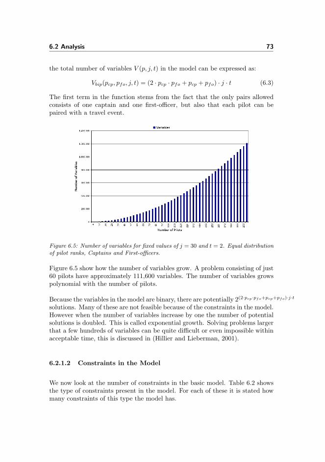
6.2 Analysis 73
the total number of variables V (p, j, t) in the model can be expressed as:
Vbip(pcp, pfo, j, t) = (2 · pcp · pfo + pcp + pfo) · j · t (6.3)
The first term in the function stems from the fact that the only pairs allowedconsists of one captain and one first-officer, but also that each pilot can bepaired with a travel event.
Figure 6.5: Number of variables for fixed values of j = 30 and t = 2. Equal distributionof pilot ranks, Captains and First-officers.
Figure 6.5 show how the number of variables grow. A problem consisting of just60 pilots have approximately 111,600 variables. The number of variables growspolynomial with the number of pilots.
Because the variables in the model are binary, there are potentially 2(2·pcp·pfo+pcp+pfo)·j·t
solutions. Many of these are not feasible because of the constraints in the model.However when the number of variables increase by one the number of potentialsolutions is doubled. This is called exponential growth. Solving problems largerthat a few hundreds of variables can be quite difficult or even impossible withinacceptable time, this is discussed in (Hillier and Lieberman, 2001).
6.2.1.2 Constraints in the Model
We now look at the number of constraints in the basic model. Table 6.2 showsthe type of constraints present in the model. For each of these it is stated howmany constraints of this type the model has.
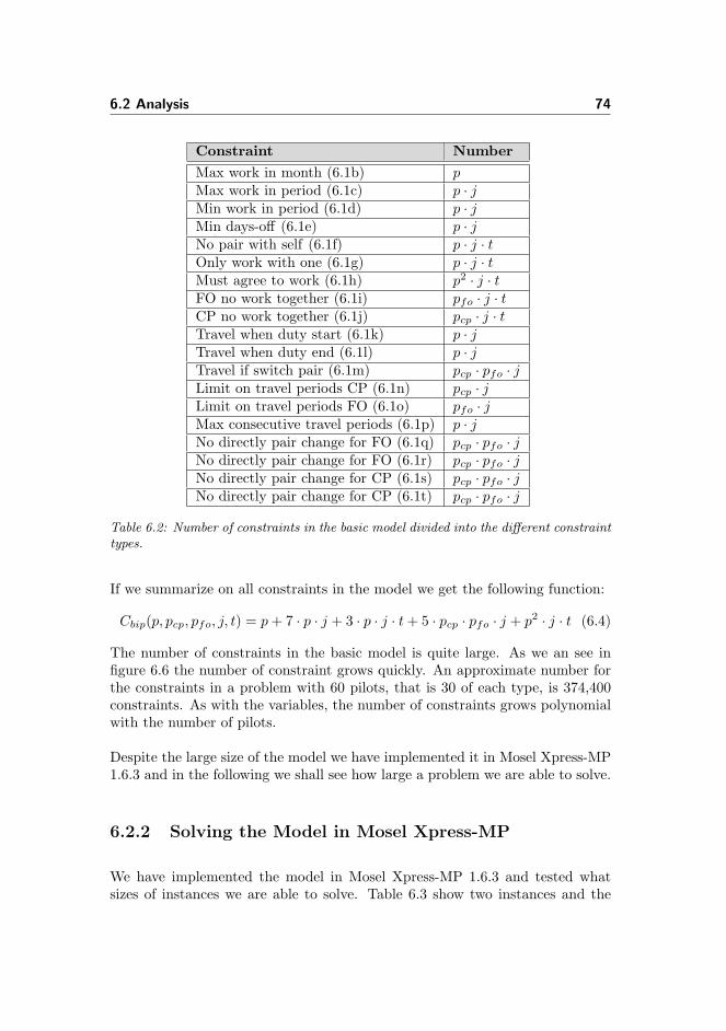
6.2 Analysis 74
Constraint NumberMax work in month (6.1b) pMax work in period (6.1c) p · jMin work in period (6.1d) p · jMin days-off (6.1e) p · jNo pair with self (6.1f) p · j · tOnly work with one (6.1g) p · j · tMust agree to work (6.1h) p2 · j · tFO no work together (6.1i) pfo · j · tCP no work together (6.1j) pcp · j · tTravel when duty start (6.1k) p · jTravel when duty end (6.1l) p · jTravel if switch pair (6.1m) pcp · pfo · jLimit on travel periods CP (6.1n) pcp · jLimit on travel periods FO (6.1o) pfo · jMax consecutive travel periods (6.1p) p · jNo directly pair change for FO (6.1q) pcp · pfo · jNo directly pair change for FO (6.1r) pcp · pfo · jNo directly pair change for CP (6.1s) pcp · pfo · jNo directly pair change for CP (6.1t) pcp · pfo · j
Table 6.2: Number of constraints in the basic model divided into the different constrainttypes.
If we summarize on all constraints in the model we get the following function:
Cbip(p, pcp, pfo, j, t) = p+ 7 · p · j + 3 · p · j · t+ 5 · pcp · pfo · j + p2 · j · t (6.4)
The number of constraints in the basic model is quite large. As we an see infigure 6.6 the number of constraint grows quickly. An approximate number forthe constraints in a problem with 60 pilots, that is 30 of each type, is 374,400constraints. As with the variables, the number of constraints grows polynomialwith the number of pilots.
Despite the large size of the model we have implemented it in Mosel Xpress-MP1.6.3 and in the following we shall see how large a problem we are able to solve.
6.2.2 Solving the Model in Mosel Xpress-MP
We have implemented the model in Mosel Xpress-MP 1.6.3 and tested whatsizes of instances we are able to solve. Table 6.3 show two instances and the

6.2 Analysis 75
Figure 6.6: Number of constraints for fixed values of j = 30 and t = 2. Equaldistribution of pilot ranks, Captains and First-officers.
solution times for these. The computer used to solve these instances is describedin section 4.6. The implementation in Mosel Xpress-MP 1.6.3 is included in
Instance Pilots (CP/FO) Solution time (hh:mm:ss)1 2 (1/1) 00:00:252 4 (2/2) Not done within 24 hours
Table 6.3: Solution time for the two instances are given in the third column. Thenumber of pilots is given for each of the instances. Number of days is 30 and numberof time periods is 2.
appendix B.1.
We can see, as was expected, that due to the size of the model we are not ableto solve even small instances. Therefore we will not move further on with thisapproach, but instead take on another well-known solution approach to the crewrostering problem which is a Multi-Commodity Network Flow approach.

Chapter 7
A Multi-Commodity NetworkFlow Model Approach
We saw in chapter 6 that when modeling the problem as a binary integerproblem, we were not able to solve even very small problems that include pairsof pilots. Another way of approaching the problem is as a network flow model.The network is constructed so a roster is a path in the network. For furtherinspiration on a multi-commodity network flow problem approach to the regularcrew rostering problem, see (Cappanera and Gallo, 2004). In this chapter wewill introduce multi-commodity network flow model for the BJARP.
First some basic definitions: a flow network is a directed graph G = (N,A)where N is the set of nodes and A is the set of arcs in the network. Each archas a capacity and can receive a flow. The graph has a source node and a sinknode. The flow can travel from the source to the sink via the directed arcs.
A flow in a network is defined as follows. An directed arc p goes from node uto node v. For each arc p = (u, v) in the network there is a variable xu,v whichis a non-negative real number, being the flow on arc (u, v), which satisfy theconditions (7.1) and (7.2). Condition (7.1) is called a capacity constraint. Itmakes sure that the flow xu,v along an arc (u, v) cannot exceed its capacity cu,v.Additionally any flow cannot be negative.
0 ≤ xu,v ≤ cu,v, ∀u, v ∈ N (7.1)

77
Condition (7.2) is called a flow conservation constraint. It states that the flowentering a node n must equal the flow going out of node n. In other words, noflow can be lost in a node. This condition should be satisfied for all nodes in thenetwork except for the source node and the sink node. The source node producesflow, so no flow comes in, but flow can exit, and the sink node consumes flow,i.e. flow enters, but no flow exits the node.∑
v∈Nxw,v =
∑v∈N
xv,w ∀w ∈ N\{s, t} (7.2)
In figure 7.1 a small network is shown.
Figure 7.1: Network, where each arc has a capacity of 1. Node s is the source nodeand node t is the sink node.
In the network node s, is the source node and node t is the sink node. The flowcan run through the arcs in the direction of the arcs as illustrated. Howeverthe flow cannot exceed the capacity of the arc it enters. We want to push flowfrom the source in the network to the sink in the network. In the example infigure 7.1 all arcs have a capacity of 1. We are hence able to push a flow of 1from the sink to the source via the following paths in the network: {s, a, c, t},{s, b, d, t}, {s, a, c, d, t}, {s, b, a, c, t} and {s, b, a, c, d, t}.
The network in the example is a single-commodity network. This means thatonly type of flow is sent through the network and that only one source and onesink node exists in the network.
For multiple commodities, let the set K define the set of commodities andcommodities be denoted k ∈ K. In a multi-commodity network flow problemthere can be several commodities sharing the same network, but having separatesources sk and sinks tk. The problem can be seen as having several goods thatneed to be transported through a network in order to arrive at their respectivedestinations. The basic definitions of the network for a single-commodity

7.1 Multi-Commodity Network Flow 78
network are also valid for the multi-commodity network flow problem. However,the following equations are used for modeling a k-commodity network flowproblem instead of equations (7.1) and (7.2).
0 ≤∑k
xku,v ≤ cu,v ∀u, v ∈ N, k ∈ K (7.3)
Like (7.1) equation (7.3) is a capacity constraint. The sum of the flow from allof the commodities cannot exceed the given capacity on an arc.∑
v∈Nxkw,v =
∑v∈N
xkv,w ∀w ∈ N\{sk, tk}, k ∈ K (7.4)
Equation (7.4) ensure the conservation of flow. The flow entering a node isrequired to equal the flow exiting the node. The constraint is valid for all nodesin the network except for the source and sink nodes.
Figure 7.2: Here the same basic network as in figure 7.1 is shown, except for thenumber of commodities. Here we now have two commodities. The arcs shared by thecommodities now have a capacity of 2, so both commodities can maintain a flow ofmaximum 1 and hence flow unrestricted.
An example of a two-commodity network is illustrated in figure 7.2. Thereare two sink nodes s1 and s2 and two source nodes t1 and t2, a pair for eachcommodity 1 and 2. For further information on the multi-commodity networkflow problem, see (Assad, 1978).
7.1 Multi-Commodity Network Flow
In this section we will represent the Crew Rostering problem for Business JetAirline with a multi-commodity network flow model. First a description of howthe network is constructed will be provided. Then we will give a basic modelthat considers a subset of the characteristics and rules mentioned in section 3.3,

7.1 Multi-Commodity Network Flow 79
these are rules [R1]-[R4] and [R7] and [R9]. In section 7.1.3 it is discussed howthe model can be further extended, these extensions include rules [R5] and [R6].We discuss the model size and how the model grows in section 7.2.1.
7.1.1 The Network
Some of the characteristics of the problem can be automatically implementedwhen constructing the network. These are explained and discussed in thissection.
We can formulate the problem as a directed graph G = (N,A). The graph hasan equal set of nodes for each time period. Here one time period is a certain day,”am” or ”pm”. The number of node sets or “time layers” in the graph is givenby the number of time periods in the planning period. The arcs represent thepossible actions to take for the pilots, at a certain time, and are always directedforward in time. The flow on an arc depends on the number of pilots allowedon the arc. The flow is always greater or equal to zero and has an upper boundwhich is the number of pilots allowed on the arc. In the following examples wewill have more than one arc between nodes for illustrative purposes. This is notreally the case but the several arcs are constructed to illustrate which pilots areallowed to travel on the arc. So the capacity of each arc is based on the numberof pilots allowed to travel on the arc. The flow on the arc equals the number ofpilots actually using the arc, as their individual flow always equals either zeroor one.
In the graph there is a sink (or origin) node for each pilot as well as a source(or destination) node, that is there is one commodity for each pilot. The nodesin the graph are activities. To begin with we divide the activities into threedifferent groups: Duty, Travel and Off-duty. For each time period there is atravel-node (TR) and a off-node (OFF). The duty nodes are constructed foreach possible pair of pilots. So the information of which pilots are workingtogether is integrated in the duty nodes. When constructing the duty nodesonly legal pairs of pilots are represented, i.e. rule [R9] regarding allowed pairsof pilots are respected. A roster for a pilot in the planning period is a path inthe network from the source representing the pilot to the sink representing thepilot.
In figure 7.3 a brief example of how the nodes are set up is shown.
In the example there are four pilots, two master pilots and two subordinatepilots. These can be paired up, so a duty node for each possible pair of pilots andfor every time period is constructed. It is stated on each duty node which pair of

7.1 Multi-Commodity Network Flow 80
Figure 7.3: The nodes represent actions in each time period. The duty nodes areconstructed for each possible pair of pilots, telling which pilots work together.
pilots is represented. With four pilots, two master pilots (only senior captains)and two subordinate pilots, four pair combinations exist. In the upcomingsection 7.2.1 we will discuss how the network grows. The time period in whicha node is located is stated above the node. In the example shown in figure 7.3we have two days divided into ”am” and ”pm”, so four time periods are shown.Another possible actions besides entering a duty with another pilot is to travelwhen beginning a duty or having the day off. We have chosen not to includethe arcs in this example but we will carefully go through how the arcs areconstructed according to our problem later in this section.
The arcs of the network represent the possible transitions, i.e. the possibleactions to be assigned in the next period. An arc represents the action on thenode it leaves in the given time period. So having flow in an arc correspondsto activating the action of the node it leaves or simply having flow through thenode.
When constructing the arcs of the graph we can use the some generalcharacteristics and rules of the problem. In this way we construct the graph soactions that are not possible to take, are simply not represented in the network.Some of the rules however cannot be transferred directly into the structure of thegraph, so these are stated separately as constraints when solving the problem.
Below a list of characteristics we are able to express in the network is given.

7.1 Multi-Commodity Network Flow 81
These will in the following be referred to as basis rules to avoid confusion withthe rules stated in section 3.3:
1. It is illegal to go directly between a duty and off-duty, there must alwaysbe a travel action in between.
2. Pilots can only start their duty in the morning, ”am” periods, representedby a travel action.
3. Pilots can only end their duty in the afternoon, ”pm” periods, representedby a travel action.
4. For double duties: Only subordinates can change pair within a dutyperiod, and this can only be done with two consecutive travel actionsin between, located ”pm” and ”am” the following day.
These basis rules can be expressed directly in the network. In the following wewill add arcs to the network gradually, shown with an example.
In figure 7.4 the nodes in a graph of a smaller example ranging four days, inother words eight time periods are shown. In this problem there are only twopilots, one master pilot and one subordinate pilot. Hence, there is only onepossible pair. The only connections shown are the connections that go out ofthe source for each of the pilots and those that enter the sinks, i.e. the actionsthat are possible in the beginning of a planning period and in the end of aplanning period.
On the first day of the planning period both pilots can either have the firstday off or they can travel. They are not able to go on or off-duty withouttraveling. Basic rule (1) states this fact. There are however some exceptionsin the beginning of a planning period. The work schedule has to correspond tothe work schedule of the previous planning period. If a pilot is part of a dutyreaching into this planning period, the duty has to be pre-assigned for the daysin question. Therefore it is necessary that the pilots enter the duty node of thesame pair as in the end of the previous planning period. This can be dealt withby pushing flow through the duty node of the pair of pilots in question for aslong as the duty is assigned last. In reality this eliminates all other possibilitiesfor the pilots, and they will hence have no other alternatives made available inthe generated network. How a planning period generally is ended is discussedin section 4.2.1.
In the following examples colors are added to the arcs in the network with thepurpose of making clear which arcs belongs to which pilot.

7.1 Multi-Commodity Network Flow 82
In figure 7.4 it is not possible to start a period with a duty. This would requirean arc from a pilot directly to the pair for which a pilot is assigned. If necessarythe arc is constructed separately and assigned to be active by pushing flowthrough. We cannot construct connections between sources and duty nodes forall pairs of pilots, as it then would make it possible for the pilots to start a dutyon day one without having to travel before doing so.
Figure 7.4: The connections in the beginning and end of a period.
Next we extend the example by creating connections between the time layers ofthe graph. This is shown in figure 7.5 where it is now possible for the pilots towork the whole period or to be off-duty throughout the period. In the example,a pilot cannot change action during the period; these possibilities will be addedlater. In the network it is illustrated that in order for the pilot to work, he hasto travel first. This is correct according to basis rule 1.
According to the basis rules 2 and 3 it should only be possible to begin a dutyby traveling in the morning. Likewise it should only be possible to end a dutyby traveling in a time period in the afternoon. In figure 7.6 connections betweenoff nodes, travel nodes and duty nodes has been constructed according to thesebasis rules. It is now possible to begin and end duty periods in the requiredtime periods. Starting or ending a duty period is always done with a travel inbetween the duty and off node, that is no direct connections between the twoactions exist.
The last type of connections that have been added in figure 7.6 compared tofigure 7.5 is between two travel actions over time periods from an evening tothe following morning. These connections now enables pilots to travel over twoconsecutive time periods, ”pm” and ”am” the following day. However it is onlya feasible action for the subordinate pilot, as the master pilot has no connection.

7.1 Multi-Commodity Network Flow 83
Figure 7.5: Connections so pilots can perform the same action over several timeperiods.
Figure 7.6: The full network over four days, without pre-assignments. Here the pilotscan change action.
This is in full correspondence with basis rule number 4.
We have now constructed a network that already express many characteristicsand rules that are problem specific. In figure 7.7 we give an illustration of thetransformation of a schedule with two rosters into a flow in our constructednetwork.
In the following section a model of the problem will be developed and explained.

7.1 Multi-Commodity Network Flow 84
Figure 7.7: The transformation of a schedule containing the rosters of two pilots intoa flow in the network (shown by the bold arcs). Note how flow into day 2 goes fromOFF to TR and half a day later to the pair. Hereafter the flow continues from pair topair node and finally on day 5 goes down to OFF through TR.
7.1.2 The Mathematical Model
In the network we were not able to express rules regarding duration of a dutyperiod and consecutive days-off. These conditions are therefore stated in themodel of the problem. We will start by describing which sets and variables areused and afterward state the model and explain the different constraints presentin the model.
In the network model we have binary decision variables, one for each arc presentin the graph. The variable represents the activity on the node the correspondingarc departs from. There are five indexes on the variables: the pilot, the eventthe pilot is assigned, the event the pilot is assigned in the subsequent time periodand finally the day and time period. An event can either be a duty, off or travel.Compared to the BIP model described in section 6.1, where a variable onlytook the value one if the pilot was on duty or traveled, a variable in the networkmodel is one if the pilot is assigned the action it represents, whether it be duty,travel or off. This fact provides new possibilities regarding how to model theproblem specific constraints, which we will return to later in this section.
In the model presented the paired tour days objection function explained insection 4.3.1 is used. An explanation of other possible objective functionscan also be found here. Using another objective function might need other

7.1 Multi-Commodity Network Flow 85
constraints than given in this model. For an overview of variables andconstraints needed for each objective function see 4.3.1 as well.
The following variables are used in the model:
xp,e1,e2,j,t :{
1 if pilot p is at event e1 in time period j, t and moves to event e2
0 otherwise
The following sets are to be used:
P All pilotsPAIR All legal pair combinations
E Events: travel (tr), off, dutyJ Days, {0, 1, . . . , ndays}T Time periods, {“am′′, “pm′′}
For rules and regulations, the constants wmax, wmin and woff are used, see

7.1 Multi-Commodity Network Flow 86
section 3.3 for more on these.
min.:∑p∈P
∑j∈J
∑t∈T
xp,duty,duty,j,t (7.5a)
st.:∑e∈E
xp,e,e,j−1,2 −∑e∈E
xp,e,e,j,1 =0
∀p ∈ P, e ∈ E, j ≥ 2 (7.5b)∑e∈E
xp,e,e,j,1 −∑e∈E
xp,e,e,j,2 =0
∀p ∈ P, e ∈ E, j ∈ J (7.5c)∑e1,e2∈E
xp,e1,e2,j,t =1
∀p ∈ P, j ∈ J, t ∈ T (7.5d)∑e∈E
xp,e,dutyp,p,j,t +∑e∈E
xp,e,dutyp,p,j,t ≥2 ·∑e∈E
xp,e,dutyp,p,j,t
∀{p, p} ∈ PAIR, j ∈ J, t ∈ T(7.5e)∑
e∈Exp,e,dutyp,p,j,t +
∑e∈E
xp,e,dutyp,p,j,t ≥2 ·∑e∈E
xp,e,dutyp,p,j,t
∀{p, p} ∈ PAIR, j ∈ J, t ∈ T(7.5f)
j+wmax∑l=j
xp,tr,off,l,2 ≥xp,off,tr,l,2
∀p ∈ P, j ∈ J (7.5g)j+wmin−1∑l=j+1
xp,tr,off,j,2 ≤1− xp,off,tr,j,2
∀p ∈ P, j ∈ J (7.5h)j+woff∑l=j+1
∑t∈T
xp,off,off,l,t ≥(2 · woff − 1) · xp,tr,off,j,2
∀p ∈ P, j ∈ J (7.5i)xp,e1,e2,j,t ∈{0, 1}
∀p ∈ P, e, e1, e2 ∈ E, j ∈ J, t ∈ T(7.5j)
7.1 Multi-Commodity Network Flow 87
In this model there is a variable for all combinations of pilots, events and timeperiods. The majority of these are set to zero as there is no possibility for anyflow. So when solving this model only the variables that actually have a possibleflow are included. The objective function is as mentioned the number of pairedtour days in the planning period. In this model the number of paired tour dayscan be found by summing the flow on the arcs from one DUTY node to another.
In the following we will describe the constraints given in this model.
As this model is a multi-commodity network flow model, flow conservationconstraints are needed. Constraints (7.5b) and (7.5c) ensure that the amountof flow in arcs in a time period for each pilot is the same as the amount of flowthat is present in the arcs in the next time period.
Constraint (7.5b) deals with the arcs that cross the days, from a ”pm” toan ”am” period. Constraint (7.5c) ensures flow conservation during the day(between an ”am” and a ”pm” time period).
Constraint (7.5d) ensures that pilots are assigned precisely one action in eachtime period.
To make sure that a pair consists of two pilots, we must ensure that both ornone of the pilots that are allowed to enter a specific pair duty does so. Herethe duty node of the pair is denoted as dutyp,p. Constraints (7.5e) and (7.5f)makes sure of this.
Remaining are the rules [R1] to [R3]. A duty period can last between three andsix days, and a duty period must be followed by an off period of at least fivedays. These conditions were also modeled in the BIP model. Because of the factthat this model is a network flow, much of the structure of a feasible solution isalready expressed in the graph. For instance it is not possible to flow directlybetween duties and off-duties. The graph has no direct connections betweenduty and off-duty, which means that constraining this, as we did in the BIPmodel, is not necessary.
Also the fact that the variables are one also when the pilots are not workingprovides new possibilities when modeling the constraints on duty duration andconsecutive days-off. These constraints will be explained in the following.
Constraint (7.5h) ensures that a duty period is no less than wmin consecutivedays. For day j the variable xp,off,tr,j,2 registers if a duty begins the followingday. If that is the case the variable will be set to one and the right side of theequation will be zero. This will force the left hand side of the equation to bezero as well. On the left hand side is a sum over variables registering the end of

7.1 Multi-Commodity Network Flow 88
a duty. The sum is over the days from the following day, where the duty startsand two days ahead. The sum gives the number of times the pilot ends a dutyin the period of time it is summarizing over. If a duty was to end two days afterit began, the sum
∑j+wmin−1l=j+1 xp,tr,off,j,2 would be one which is not possible.
Figure 7.8: Constraining minimum working days in the network model; wmin = 3.The bold arcs show the flow in the network, red arcs the path that becomes infeasibleand the arc with ”no entry” sign mark the arc that constraint (7.5h) prohibits. A showsan illegal path and B shows a legal.
In figure 7.8 the network for five days for one pilot is shown. The bold arcsrepresent the arcs that have contains flow. The red arcs have a ”no entry”sign across. These arcs cannot contain flow because of constraint (7.5h). Arc Arepresents ending a two days duty, which is not possible. Hence the first possibletime to end a duty is three days after it began, illustrated by B.
The second rule regarding duration of working period, is that a duty period isnot allowed to exceed wmax = 6. This rule is expressed by constraint (7.5g).The idea of the constraint is somewhat the same as for the constraint ensuringminimum wmin = 3 consecutive working days. Again we exploit that we areable to register how many times in a given period of time a pilot starts and endsa working period. On the left hand side of the equation we sum up the numberof times a given pilot ends a duty in a time period that is seven days long. Wewould like this sum to be equal to one if the pilot started working on day oneof the time period. The variable xp,off,tr,l,2 equals one if this is the case. So ifa pilot started a duty constraint (7.5g) forces the pilot to end his duty periodwithin wmax = 6 days. If the pilot does not start a duty period on the day inquestion, xp,off,tr,l,2 equals zero and the sum is also allowed to be zero.
We have illustrated the effect of constraint (7.5g) in figure 7.9 for one pilot. Herewe look at a period of eight days, except for the last period of day eight. On dayone the pilot is off-duty. On day two the pilot starts his duty by traveling andthen enters a duty node in the following time period. This makes the variablexp,off,tr,1,2 = 1, that is, pilot p is no longer off duty but starts traveling in the

7.1 Multi-Commodity Network Flow 89
Figure 7.9: Constraining maximum working days in the network model; wmax = 6. Thebold arcs show the flow in the network, red arcs show the path that becomes infeasibleand the arc with the ”no entry” sign mark the flow that constraint (7.5g) prohibits.
next time period, which in this case is in the morning on day two. He shouldthen be on duty at most six consecutive days, hence the last possible time toexit the duty is at day 1 + wmax = 1 + 6 = 7. This means that the sum overvariables for each day indicates if the pilot exited the duty period before dayeight. In figure 7.9 it is shown that exiting the duty period at day eight is notpossible, illustrated by B. But it is possible to exit on day seven, that is thesixth day in the duty period, shown by A.
That completes the constraints on the duration of the duty periods. Whatremains now is to make sure the pilots have at least five consecutive days-offafter a duty period. Constraint (7.5i) covers this. We start by looking at aspecific day, for a given pilot. On the right hand side, the variable xp,tr,off,j,2,which is one if the pilot p was working and ended his duty on day 1. Thisvariable is multiplied with (2 · woff − 1) = 9. On the left hand side in theequation we sum up the number of time periods the pilot has been off-duty. Wewould like this sum to be at least five days. The sum starts one time period intothe off duty period, so the number of time periods the pilot at least should haveis nine. Hence, if the pilot ended his shift on the day in question, constraint(7.5i) now ensures that the pilot has at least five following consecutive days offafterward.
Figure 7.10 illustrates the effect of constraint (7.5i). Again the network is shownfor one pilot, here over a seven-day-period. The bold arcs show the flow in thenetwork, and the red arcs show the possible flow that is now prohibited byconstraint (7.5i). It is not possible to start a new duty period on day six, wherethe pilot has had four consecutive days-off. At day seven it is possible to starta new duty by traveling, but the pilot can also continue to be off-duty.

7.1 Multi-Commodity Network Flow 90
Figure 7.10: Constraining minimum consecutive days-off after a duty period in thenetwork model; woff = 5. The bold arcs show the flow in the network, red arcs showthe path leading to the flow that constraint (7.5i) prohibits, illustrated with the ”noentry” signs.
Variables and constraints regarding source and sink nodes are not a part of themodel simply because they are not needed. By ensuring that the flow crossingeach time period and hence between the two first time periods is one for eachpilot, we have imposed flow on exactly one arc between the two periods. Soactually the nodes in the first time unit in the model act as source nodes.Likewise the nodes in the last time unit in the model acts as sink nodes.
This concludes the basic mathematical model of the problem. In the next sectionwe will discuss how to potentially extend the model further. We have chosennot to model and implement extensions. These are part of the problem, butas we will see when discussing the size of the model in section 7.2.1, the modelis already too large to solve for real life instances. Therefore we have chosento discuss how to extend the model rather than doing so and implementingextensions.
7.1.3 Extensions
The network model we have described in section 7.1 can be extended to includemore problem specific rules and characteristics. In this section we will describehow to include some more features in the network model. Some of the featureswe have not included in the basic model are listed below, followed by a discussionof the possibilities of including these.

7.1 Multi-Commodity Network Flow 91
• Pre-assignments.
• Maximum working days in a month and in a quarter, rules [R5] and [R6].
Pre-assignments:We can easily include pre-assignments in the model. The pre-assignmentscan be different events, such as vacation and different training courses. Mostimportantly, pre-assignments are events that cannot be registered with theevents we already have present in the existing model. They are events thatare considered as individual, that is, the pilot is not part of any pair.
Pre-assignments can be implemented in the model by adding additional nodesand arcs to the network. For each time period a new node is added. Thisnode then represents a pre-assignment. Arcs crossing the time periods areestablished between the pre-assignment nodes. Arcs connecting off nodes tothe pre-assignment nodes are also established as well as arcs between the travelnodes and the pre-assignment nodes. There are no connections between dutynodes and pre-assignments, as it is not possible to end a duty without traveling.In figure 7.11 we have illustrated how the pre-assignment nodes are created andconnected to the rest of the network. The new arcs are highlighted in the figure.
Figure 7.11: The pre-assignment nodes are constructed and connections are established.The arcs showed are the newly constructed ones, while the rest of the connections inthe network are left out.
The construction of the connection between a pre-assignment node and a travelor an off node, now make it possible for a pilot to enter and exit a pre-assignment.The connections are constructed so a pilot can enter a pre-assignment in the

7.1 Multi-Commodity Network Flow 92
morning, during ”am” period, and exit a pre-assignment in a ”pm” period.Connections between pre-assignment nodes are also established.
When solving the problem we can assign a pilot to a pre-assignment bypushing flow through the arcs that represent the action at a specific time.When constructing the network only flow on the arcs complying with the pre-assignment are allowed. The capacity on the other arcs in the same time periodsas the pre-assignment are set to zero.
The pre-assignment event is added to the event set E in the model. The flowconservation constraints (7.5b) and (7.5c) also apply for this new part of thenetwork. There should still only be one action per time period, and the flow intoa pre-assignment node is, similar to the other event nodes, equal to the flow outof the node. Constraint (7.5d) also holds when the pre-assignment is includedin the set of events. As there are no arcs between duty arcs and pre-assignmentarcs constraints (7.5e) and (7.5f) are not affected. Constraints (7.5g), (7.5h) and(7.5i) should not apply for pre-assignments. The pre-assignments could very wellhave a duration of more than six days. These constraints therefore have to applyto a subset of all events, which is all events excluding pre-assignments.
If the pre-assignment is an exercise session, five consecutive days-off of coursemust follow, as well as five days-off directly before the exercise, however as itis a pre-assignment the duration and placement would be known prior to theconstruction of the schedule. So five consecutive days-off can be guaranteed bypushing flow through the OFF → OFF arcs for five days after or before thepre-assignment has ended/begun.
However if a exercise session lasts between one and three days another duty canlegally be placed prior to or after the exercise session. Figure 7.12 illustrateshow this feature can be included. Here, an exercise sesion is pre-assigned forthe two only pilots, Joe (CP) and Ben (FO). It can be seen how the flow can ondays 4-6 only move along the arcs between pre-assignment nodes. Before andafter the pre-assignment it is possible to create a duty of length three. If oneof these duties are assigned, then the buffer ensures that the duty on the otherside of the exercise session cannot be initiated.
Another feature is also illustrated in figure 7.12: When it is known that it isonly possible to plan a duty of a certain length, it is possible to remove thepossibility for flowing on arcs, that under all circumstances would render thesolution infeasible. The flow on the new arcs to and from a pre-assignment nodeare as all other flows allowed to be either zero or one, and hence constraint (7.5j)is also applicable for the new set of events that include pre-assignments.

7.1 Multi-Commodity Network Flow 93
Figure 7.12: Depiction of an exercise session pre-assigned for two pilots transformedinto the structure of the network. Observe how it is only possible to flow among pre-assignment arcs on days 4-6.
Maximum working days in a month and in a quarter:We now move on to the administration of limits on the maximum number ofworking days. Pilots have limits on the number of working days allowed in amonth and in a quarter. These limits are specifically mentioned in rule [R5] and[R6]. To comply with the monthly rule a counting of work days is necessary.Work days can be account for by counting flow values on the arcs leading into anevent that is regarded as work. Which events are regarded as work is described insection 5.2. Pre-assigned work can be counted separately as this work is knownprior to the construction of the schedule. A new constraint in the model thenensures that the number of days counted does not exceed the allowed numberof working days.
When dealing with a planning period of a month, information regarding thenumber of working days for each pilot the past two months are needed in orderto comply with the quarterly rule. The rule can be stated in the same way asfor the monthly rule. The number of days worked in the previous two monthsis simply added to the number of working days in the planning month, and thissum then has to be less than the limit stated by the quarterly rule.

7.2 Analysis 94
7.2 Analysis
Now we have seen how to model the problem as a Multi-Commodity NetworkFlow. However because of the large amount of possible pairs of pilots the modelgrows very quickly. In this section we will analyze further on the size of themodel, the variables as well as the constraints. Like for the BIP model wewill attempt to optimally solve some instances of the problem varying in size,with the use of Mosel Xpress-MP 1.6.3. Specifications for the computer used tosolve these instances are provided in section 4.6. We will report which sizes ofproblems we are able to solve.
7.2.1 Discussion of Model Size
In this section we will discuss the size of the model presented in section 7.1.2and how it evolves with the number of pilots and thereby also the number ofpossible pairs of pilots.
The number of variables in the model equals the number of possible flows inthe network we have constructed. The number of variables is largest whenno pre-assignments are present. We will not include any pre-assignments, andhence consider the network of the basic model without pre-assigned duties inthe beginning of a month. This corresponds to not having any duties in theplanning period that were assigned in the previous planning period. By doing sothe calculation of the number of variables in the model is a worst case scenario.In the following we will determine the number of variables in the model bylooking at the possible flows in the network. Additionally we will look at thenumber of constraints in the model.
7.2.1.1 Number of Variables in the Model
In table 7.1 an overview of the variables in the model is provided. The star,” ∗ ” indicates that all variations of these settings are considered. In the secondcolumn the arcs with the possible flow corresponding to the variables are stated.Formulas for the number of possible flows and thereby the number of variablesare presented in the last column. We explain on how we have derived these

7.2 Analysis 95
formulas in the following. We use the following parameters:
p The number of pilotsb The number of all possible pairs of pilotsj The number of days in the planning periodt The number of time periods in a day
These parameters are set according to any problem in question.
Variables Arcs Possible flows
x∗,TR,TR,∗,∗ TR→ TR j·t2 · (p− 1)
x∗,TR,DUTY,∗,∗ TR→ DUTY j·t2 · p
x∗,DUTY,TR,∗,∗ DUTY → TR j·t2 · p
x∗,TR,OFF,∗,∗ TR→ OFF j·t2 · p
x∗,OFF,TR,∗,∗ OFF → TR j·t2 · p
x∗,OFF,OFF,∗,∗ OFF → OFF ((j · t)− 1) · px∗,DUTY,DUTY,∗,∗ DUTY → DUTY ((j · t)− 1) · 2 · b
Table 7.1: Number of variables/possible flow in the model divided into different arcs inthe network. A ”∗” in the stated variables indicate that all possible values are included.
TR → TR:In the network there is a TR node for every day and every time periodin the planning period which equals j · t time units. Only arcs from TRnodes located in an ”am” time period have an arc to the following TR nodelocated in the following ”pm” time period. Hence there are j·t
2 TR→ TRarcs in the network. The pilots that can use the arc are the subordinatepilots of all possible pairs. Assuming seniority all pilots except for one pilotcan assume rank of subordinate. So the possible flow on one TR → TRarc equals the number of pilots minus one, that is p− 1. Multiplying thenumber of possible flows on one arc with the number of TR → TR arcsin the network gives us j·t
2 · (p− 1) which is the number of possible flowson all TR→ TR arcs in the network.
TR → DUTY and DUTY → TR:The TR → DUTY arcs are present between all TR nodes in an ”am”period and DUTY nodes in the following ”pm” period. In the networkthis sums to j·t
2 arcs. The flow on each arc is the same as for any otherTR→ DUTY arc. All pilots have possible flow on an TR→ DUTY arc,so the possible flow on all these arcs in the network equals j·t
2 · p. Theargumentation and calculation is equivalent to those of the DUTY → TRarcs. These are also only present between an ”am” and a ”pm” timeperiod, and also have a possible flow for all pilots. Ergo the number ofpossible flows on the TR→ DUTY arcs also amounts to j·t
2 · p.

7.2 Analysis 96
TR → OFF and OFF → TR:TR→ OFF and OFF → TR arcs also have the same number of possibleflows as TR → DUTY and DUTY → TR arcs. However, here the arcsare only present in the network between an ”pm” period and the following”am” period. Also here possible flow for each pilot exists. The totalnumber of possible flows for TR→ OFF arcs therefore equals j·t
2 · p andequivalent for OFF → TR arcs the possible flow equals j·t
2 · p.
OFF → OFF :OFF → OFF arcs exist between all OFF nodes followed by another offnode in the next time unit. There are j ·t OFF nodes in the network whichgives a total of (j · t)− 1 OFF → OFF arcs in the network. Possible flowon the arcs exists for all pilots. This gives a total of ((j · t)− 1) · p possibleflows on the OFF → OFF arcs in the network.
DUTY → DUTY :For each pair of pilots there is a DUTY node in each time unit. AllDUTY nodes have arcs entering the DUTY node in the next time unitin the network. The possible flow on a DUTY → DUTY arc equals two,one flow for each pilot in the pair. This gives us a total of ((j · t)− 1) · b · 2possibles flows on all DUTY → DUTY arcs in the network.
The total number of variables is a function of the number of pilots, number ofpairs, number of days and the number of time periods in a given problem. Usingthe formulas found for each arc type we can conclude that for any given problemthe total number of variables V (p, b, t, j) in the model can be expressed as:
Vnet(p, b, j, t) =j · t2· (4 · p+ (p− 1)) + (j · t− 1) · (2 · b+ p) (7.6)
The function depends on four variables. Besides this fact, the number of pairshighly depends on the number of pilots and the distribution of pilot rank in thepilot group also illustrated by equation (4.6) in section 4.4.1.
To see how the number of variables grows with the number of pilots and pairswe have fixed the values for the number of days and number of time periods.The variables are fixed to j = 30 and t = 2. We assume that we have an equaldistribution of pilot ranks such that there are an equal number of Captains (bothnormal and low-timers) and First-Officer (both normal and low-timers). Valuesof the resulting number of variables are shown in figure 7.13. Only numbers ofpilots divisible by four are illustrated.
An example of a problem represented in figure 7.13 could be a problem with 60pilots, equally distributes so there are 15 normal captains, 15 low-timer captains,
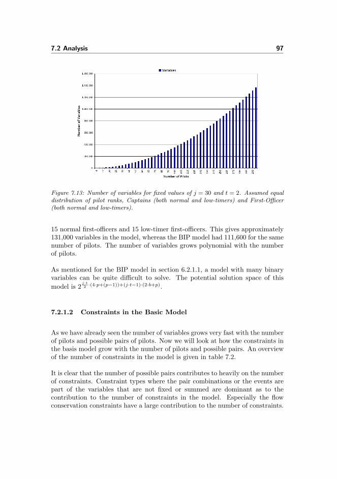
7.2 Analysis 97
Figure 7.13: Number of variables for fixed values of j = 30 and t = 2. Assumed equaldistribution of pilot ranks, Captains (both normal and low-timers) and First-Officer(both normal and low-timers).
15 normal first-officers and 15 low-timer first-officers. This gives approximately131,000 variables in the model, whereas the BIP model had 111,600 for the samenumber of pilots. The number of variables grows polynomial with the numberof pilots.
As mentioned for the BIP model in section 6.2.1.1, a model with many binaryvariables can be quite difficult to solve. The potential solution space of thismodel is 2
j·t2 ·(4·p+(p−1))+(j·t−1)·(2·b+p).
7.2.1.2 Constraints in the Basic Model
As we have already seen the number of variables grows very fast with the numberof pilots and possible pairs of pilots. Now we will look at how the constraints inthe basis model grow with the number of pilots and possible pairs. An overviewof the number of constraints in the model is given in table 7.2.
It is clear that the number of possible pairs contributes to heavily on the numberof constraints. Constraint types where the pair combinations or the events arepart of the variables that are not fixed or summed are dominant as to thecontribution to the number of constraints in the model. Especially the flowconservation constraints have a large contribution to the number of constraints.

7.2 Analysis 98
Constraint NumberFlow constraint (7.5b) p · e · (j − 1) · tFlow constraint (7.5c) p · e · j · tOne action (7.5d) p · j · tBoth or none (7.5e) b · j · tBoth or none (7.5f) b · j · tMax work (7.5g) p · jMin work (7.5h) p · jMin off (7.5i) p · j
Table 7.2: Number of constraints in the model divided into the different constrainttypes.
Figure 7.14: Number of constraints for fixed values of j = 30 and t = 2. Assumed equaldistribution of pilot ranks, captain, normal and low-timer and first-officer, normal andlow-timer.
If we summarize on all constraint in the model we get the following function:
Cnet(p, b, e, j, t) = p · e · (j − 1) · t+ p · e · j · t+ p · j · t+ 2 · b · j · t+ 3 · p · j (7.7)
The function depends on five variables. The events e highly depends on thenumber of pairs in the problem. It consists of duties for all possible pairs, traveland off. Hence we can write e = b+ 2. As for the number of variables we haveillustrated how the number of constraints grows with the number of pilots andpossible pairs. Again the values for j and t are fixed to j = 30 and t = 2. Thesame number of pilots and the distribution of the pilots are used.

7.2 Analysis 99
Figure 7.14 illustrates the growth of the number of constraints in the basicmodel. For 60 pilots there are 7,259,000 constraints, whereas the BIP modelhad 374,400 for the same number of pilots. The number of constraints growspolynomial with the number of pilots.
7.2.2 Solving the Model in Mosel Xpress-MP
We have implemented the basic model in Mosel Xpress-MP 1.6.3. For easewe assume that the pilots in the model have the following distribution: Allthe Captains have low-timer rank while all First-officers have normal status.Both categories have the same amount of pilots. This distribution only allowspairs consisting of one captain and one first-officer. In table 7.3 three probleminstances are described and the solution time for each instance are stated.Because we have no pre-assignment, the model is solved using the objectivefunction for sum of negative deviation, described in section 4.3.1.2. The demandis in all instances set to 2 pair of pilots each day.
Instance Pilots (CP/FO) Solution time (hh:mm:ss)1 4 (1/1) 00:00:012 4 (2/2) 00:00:523 6 (3/3) 01:30:224 10 (5/5) Not done within 24 hours
Table 7.3: Solution time for three instances are given in the third column. The numberof pilots are given. Equal distribution between low-timer captains and normal first-officers, no pilots with different rank in the problems. Number of days is 30 andnumber of time periods is 2.
The implementation in Mosel Xpress-MP 1.6.3 is included in appendix B.2.
It is interesting to see that it actually is possible to solve larger problems withthe Multi-Commodity Network Flow Approach when comparing to the BinaryInteger Problem Approach, see 6.2.2. When comparing the number of variablesand constraints by the theoretical derivations in both chapters we see thatthere are less of both in the Binary Integer Problem. We believe that the factthat larger problems can be solved with the Multi-Commodity Network FlowApproach is caused by the structure difference of the problem. Possibly thesolver is able to take advantage of the problem structure more for the networksthan for the binary integer problems.

Chapter 8
Simulated Annealing - AHeuristic Approach
Due to the size of the solution space and the consequential difficulty hereofin finding an optimal solution we have implemented a heuristic approach forfinding a solution within a very short time.
A general and widely used approach to combinatorial optimization problemsis local search algorithms, see (Aarts et al., 2005). There are many differenttypes of local search algorithms, but they all share the same basic idea of aneighborhood function. This function is used to render neighbors of a givensolution, which then can be considered as replacement solutions. A neighboris the given solution modified with a small change (or large depending on theneighborhood definition). When or if one of these neighbors is accepted, thealgorithm moves to the corresponding solution and then considers its neighbors.In this iterative way the algorithm moves toward desired solutions. Theadvantage with the idea of neighborhoods is that the new solution in eachiteration does not have to be constructed from square one, but just movesfrom solution to solution through the neighbors. And often in application goodsolutions are “close to each other”.
One of the most basic local search algorithms is Hill Climbing, which simplyalways selects the best neighbor in the neighborhood. However, this does not
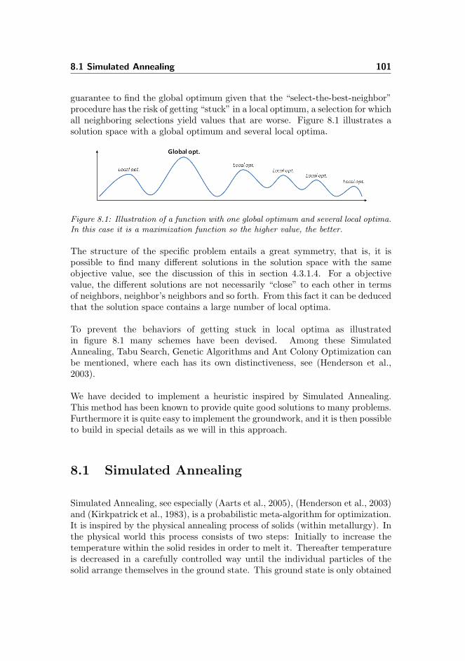
8.1 Simulated Annealing 101
guarantee to find the global optimum given that the “select-the-best-neighbor”procedure has the risk of getting “stuck” in a local optimum, a selection for whichall neighboring selections yield values that are worse. Figure 8.1 illustrates asolution space with a global optimum and several local optima.
Figure 8.1: Illustration of a function with one global optimum and several local optima.In this case it is a maximization function so the higher value, the better.
The structure of the specific problem entails a great symmetry, that is, it ispossible to find many different solutions in the solution space with the sameobjective value, see the discussion of this in section 4.3.1.4. For a objectivevalue, the different solutions are not necessarily “close” to each other in termsof neighbors, neighbor’s neighbors and so forth. From this fact it can be deducedthat the solution space contains a large number of local optima.
To prevent the behaviors of getting stuck in local optima as illustratedin figure 8.1 many schemes have been devised. Among these SimulatedAnnealing, Tabu Search, Genetic Algorithms and Ant Colony Optimization canbe mentioned, where each has its own distinctiveness, see (Henderson et al.,2003).
We have decided to implement a heuristic inspired by Simulated Annealing.This method has been known to provide quite good solutions to many problems.Furthermore it is quite easy to implement the groundwork, and it is then possibleto build in special details as we will in this approach.
8.1 Simulated Annealing
Simulated Annealing, see especially (Aarts et al., 2005), (Henderson et al., 2003)and (Kirkpatrick et al., 1983), is a probabilistic meta-algorithm for optimization.It is inspired by the physical annealing process of solids (within metallurgy). Inthe physical world this process consists of two steps: Initially to increase thetemperature within the solid resides in order to melt it. Thereafter temperatureis decreased in a carefully controlled way until the individual particles of thesolid arrange themselves in the ground state. This ground state is only obtained

8.1 Simulated Annealing 102
when the maximum value of the temperature has been sufficiently high and thecooling phase has been sufficiently slow.
Transferring this analogy to solving a combinatorial optimization problem leadsto a meta-algorithm (however it is a quite weak analogy). During optimizationit accepts improvements in cost, yet will also accept worsening to a limitedextent. The result of the high starting temperature that is carefully cooledthroughout the procedure is an algorithm which in the beginning acts likea randomized search and gradually converging toward a local search with adecreasing probability for escaping the local area.
When implementing a Simulated Annealing-based approach, the following threebasic components have to be considered: Choice of neighborhood(s), Choice ofstarting temperature and a Cooling Schedule. In this section and subsectionswe will go into details with these three components.
The pseudo-code for our implementation of Simulated Annealing is found inthe algorithm listing 8.1. Within this listing three other procedures are used:Energy calculates the energy of a solution; FindNeighbor (see listing 8.3)finds a neighboring solution; GetProbabilityForMove (see listing 8.2) findsthe probability for moving to a neighboring solution given its energy, the energyof the current solution, the progress express as a fraction of the entire runningtime and the starting temperature.
Algorithm 8.1 Pseudo-code for Simulated Annealing, inspired by (Aarts et al.,2005) and (Henderson et al., 2003).Require: Initial solution s0, Starting temperature Tstart, Running time ttotal
1: scurrent := s0, ecurrent :=Energy(s)2: sbest := scurrent, ebest := ecurrent3: while telapsed < ttotal do4: Tcurrent = Tstart(1− telapsed
ttotal)
5: sneighbor := FindNeighbor(scurrent)6: eneighbor := Energy(sneighbor)7: if eneighbor is better than ebest then8: sbest := sneighbor, ebest := eneighbor9: end if
10: if GetProbabilityForMove(ecurrent, eneighbor, Tcurrent) > random in[0, 1) then
11: scurrent := sneighbor, ecurrent := eneighbor12: end if13: end while14: return sbest
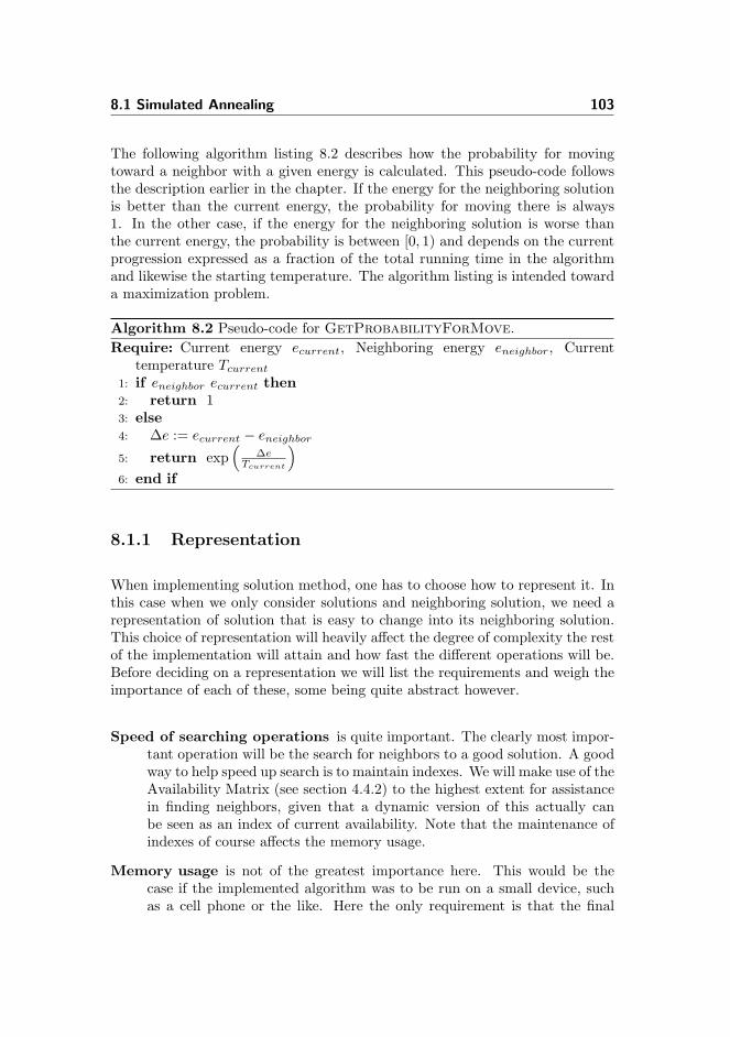
8.1 Simulated Annealing 103
The following algorithm listing 8.2 describes how the probability for movingtoward a neighbor with a given energy is calculated. This pseudo-code followsthe description earlier in the chapter. If the energy for the neighboring solutionis better than the current energy, the probability for moving there is always1. In the other case, if the energy for the neighboring solution is worse thanthe current energy, the probability is between [0, 1) and depends on the currentprogression expressed as a fraction of the total running time in the algorithmand likewise the starting temperature. The algorithm listing is intended towarda maximization problem.
Algorithm 8.2 Pseudo-code for GetProbabilityForMove.Require: Current energy ecurrent, Neighboring energy eneighbor, Current
temperature Tcurrent1: if eneighbor ecurrent then2: return 13: else4: ∆e := ecurrent − eneighbor5: return exp
(∆e
Tcurrent
)6: end if
8.1.1 Representation
When implementing solution method, one has to choose how to represent it. Inthis case when we only consider solutions and neighboring solution, we need arepresentation of solution that is easy to change into its neighboring solution.This choice of representation will heavily affect the degree of complexity the restof the implementation will attain and how fast the different operations will be.Before deciding on a representation we will list the requirements and weigh theimportance of each of these, some being quite abstract however.
Speed of searching operations is quite important. The clearly most impor-tant operation will be the search for neighbors to a good solution. A goodway to help speed up search is to maintain indexes. We will make use of theAvailability Matrix (see section 4.4.2) to the highest extent for assistancein finding neighbors, given that a dynamic version of this actually canbe seen as an index of current availability. Note that the maintenance ofindexes of course affects the memory usage.
Memory usage is not of the greatest importance here. This would be thecase if the implemented algorithm was to be run on a small device, suchas a cell phone or the like. Here the only requirement is that the final

8.1 Simulated Annealing 104
product should be able to run on a average personal computer. Howeverone should of course be aware of memory usage, as it is a factor.
We will choose the following representation which is inspired by the way thebinary integer problem was modeled (see section 6.1), but with the binary partremoved and diverged in several ways.
First we use a npilots×ndays×nperiods matrix solution representing the currentsolution. Each cell in the matrix can attain the following values:
• A number corresponding to the pilot with whom the duty is paired with.
• The begin or end of duties, TRbegin or TRend which will be representeddifferently depending on whether it is a duty for a master pilot orsecondary pilot in a single duty or master pilot, first or secondary pilotsin a double duty.
• An EMPTY value denoting no assignment.
Please note that this matrix cannot contain any other values, positions “locked”by pre-assignments and such are set to EMPTY and will be maintained by thedynamic Availability Matrix. This matrix enables direct lookup of the activityof a given pilot on a given day and time period.
To avoid having to search through the entire matrix of assignments to find aduty, a dynamic list with reference entries is used. An entry in this list containsenough information to find a duty in the above matrix solution, being themaster pilot and the days involved (denoted by starting and ending day). Sincethe overall goal of this list is to be able to find a duty without searching throughthe matrix, some information about the duty is not stored: secondary pilotsand the day of change for secondary pilots in a double duty are not saved inthe entry. However, this information can still be found easily, the entry in thelist provides the information necessary to make a direct look-up in the matrixto find the rest of the information about the duty.
8.1.2 Choice of Neighborhood
So far we have only mentioned the notion of a neighborhood. All the neighborsin a neighborhood are with other words the candidate moves from a solution. Inorder to stick with the idea of Simulated Annealing, it should both be possibleto find neighbors that improve of the current solution, yet also find neighbors

8.1 Simulated Annealing 105
that worsen the objective value. In this implementation we have chosen todefine our neighborhood as consisting of “sub-neighborhoods”. We categorizeour sub-neighborhoods to be either constructive or destructive. A constructivesub-neighborhood is defined as a sub-neighborhood where the selection of anygiven neighbor within will always keep or improve the previous objective valueand never worsen it. A destructive sub-neighborhood is defined as the opposite,a selection of a neighbor within will always keep or worsen the previous objectivevalue and never improve it.
Our three “sub-neighborhoods”, CreateSingleDuty that creates a singleduty, CreateDoubleDuty that creates a double duty and DeleteDuty thatdeletes a duty will be described in the following sections.
8.1.2.1 Constructive Sub-Neighborhood: CreateSingleDuty
This sub-neighborhood consists of neighbors where an extra single duty has beeninserted.
A single duty is located in a two step procedure. Initially a candidate for masterpilot is found by searching in the dynamic Availability Matrix. Hereafter acandidate for subordinate pilot is found which should match the found masterpilot candidates’ duty length.
There are two possible results from requesting this sub-neighborhood for aneighbor. Either a neighbor with a new single duty is selected or nothinghappens. The second will only occur in the case where the search algorithmwas unable to find any placements for a new single duty.
8.1.2.2 Constructive Sub-Neighborhood: CreateDoubleDuty
This sub-neighborhood consists of neighbors where an extra double duty hasbeen inserted.
A double duty is located in a three-step procedure. This procedure is quitesimilar to the two-step procedure to find a single duty. Initially a candidatefor one subordinate pilot with a limited available duty length in the dynamicAvailability Matrix is found. This length should be between wmin and wmax−wmin + 1. Hereafter a candidate for master pilot covering the found duty of thesubordinate pilot is found. Finally a second subordinate pilot is found to coverthe part of the master pilot’s duty not covered by the first found subordinate

8.1 Simulated Annealing 106
pilot.
There are two possible results from requesting this sub-neighborhood for aneighbor. Either a neighbor with a new double duty is selected or nothinghappens. The second will only occur in the case where the search algorithm wasunable to find any placements for a new double duty.
8.1.2.3 Destructive Sub-Neighborhood: DeleteDuty
The DeleteDuty is a destructive sub-neighborhood which is introduced inorder to make it possible for the heuristic to move from a current solution toa worse solution. A random duty is selected and removed from the currentsolution.
There are two possible results from requesting this sub-neighborhood for aneighbor. Either a random neighbor is selected and removed or nothing happens.The second will only occur in the case where the solution is empty.¨
8.1.2.4 Suggestions for Other Sub-Neighborhoods
We will briefly present some suggestions for other sub-neighborhoods thatwould be interesting to examine in future work. We will justify our choiceof implemented sub-neighborhoods.
Of neighborhoods that are related directly to duties, it would be possible toimplement the following: Shrink-a-duty, Enlarge-a-duty or Move-a-duty. Theshrinking neighborhood would be regarded as a destructive neighborhood whilethe enlarging neighborhood would be classified as a constructive neighborhood.The moving neighborhood would only make sense to implement, when theobjective function was LND. Here moving to a neighbor could potentially returna different solution value. For the objective functions PTD and SoND all possibleneighbors when moving duties would all have the same value.
If more information on the value of a certain pilot being in a pair was available,it would be possible to implement neighborhoods such as swapping one or twopilot within. Currently, this neighbor would have the same problem as theMove-a-duty, here all objective function would have the same value before andafter a swap of pilots in a duty.
We have chosen to implement our three neighborhoods, CreateSingleDuty,

8.1 Simulated Annealing 107
CreateDoubleDuty and DeleteDuty because they cover most possibilities.Move-, shrink- and enlarge-a-duty are all covered with two steps. First a dutyis deleted and then reconstructed in its new form. Of course the possibility forthe duty to be moved one day would be much more likely with a single move-operation than with a two-step, delete-and-create-operation would. If moreinformation on values of choosing certain pilots or certain days were available,it would be possible to implement more neighborhoods.
8.1.2.5 Probabilities for Choice of Neighborhoods
In reality the three selected sub-neighborhoods are joined together to resembleone single merged neighborhood. Within this merged neighborhood, individualprobabilities are assigned each of the sub-neighborhoods, denoting the prob-ability of selection of a neighbor from each of the sub-neighborhoods. Theseindividual probabilities {psingle, pdouble, pdelete} will be subject to parametertuning and specific values are therefore not to be mentioned here. Howeverit is possible to give short discussion of a condition that must always be trueand a rule of thumb for the selection of individual probabilities.
Algorithm 8.3 Pseudo-code for FindNeighbor.Require: Solution s, Probabilities psingle + pdouble + pdelete = 1
1: r ← random number in interval [0, 1)2: if r < psingle then3: return sneighbor := FindCreateSingleDutyNeighbor(s)4: else if r < psingle + pdouble then5: return sneighbor := FindCreateDoubleDutyNeighbor(s)6: else7: return sneighbor := FindDeleteDutyNeighbor(s)8: end if
As a general rule, the sum of all probabilities must cover the entire probabilityspace. In other words the sum must always add up to 1: psingle + pdouble +pdelete = 1 in this implementation given a standard probability space between0 and 1.
A rule of thumb for choosing probabilities is to give the heuristic a realisticpossibility for converging toward a good solution (for a discussion of what agood solution is, see section 3.2. This will be the case when there is a higherprobability for selecting a neighbor in a constructive neighborhood than in adestructive neighborhood. In this implementation it will entail that the sum ofprobabilities for the constructive neighborhoods should be selected to be largerthan sum of probabilities for the destructive neighborhoods. In other words,

8.2 Experimental Results 108
select probabilities so psingle + pdouble > pdelete is true. However it should benoted that if this condition does not hold it does not say that it is not possibleto find a good solution – simply that that the heuristic will not be likely toconverge as well toward the optimal solution.
8.1.3 Choice of Cooling Schedule
There are many possibilities for choice of cooling schedule for SimulatedAnnealing, see (Nourani and Andresen, 1998). Initially one must decide whetheror not the temperature should end at zero or not. If chosen, it will mean thatin the iteration(s) where the temperature is zero, the probability of selectingworse solution will be zero as well. Furthermore one has to chose the rate of thedecrease in temperature, in other words the cooling schedule. Possibilities hereare for example: Exponential, T (t) = T0α
k, where k is the step count. Linear,T (t) = T0(1 − k
kmax), where kmax is the maximal steps, as well as logarithmic
and various other possibilities.
In this implementation we choose to apply a linear cooling schedule. We dothis as we have no information on which choice of cooling schedule would besuitable for our problem. Therefore, we make the choice on another basis: byselecting a linear cooling schedule, we remove a parameter for the parametertuning. Of course, in future work, it could be interesting to look into othercooling schedules. Furthermore, we decide that the end temperature in the finaliteration should be 0, i.e. Tend = 0.
8.2 Experimental Results
This section is divided into two main parts. First the tuning of the SimulatedAnnealing in order to find the best settings for the parameters, and secondtesting and solutions with the best parameter settings found in the tuning part.
When tuning and testing a heuristic or any algorithm for that matter, it iscritical that the datasets used for tuning are not the same as the sets usedfor testing and finally for solutions. If this was the case, the algorithm wouldbe tuned as well as possible to the parameter tuning sets and hereafter testedon the same sets. Of course this would give an unrealistic performance of thealgorithm.
As commented on earlier, we have decided to divide our experiments with the

8.2 Experimental Results 109
heuristic into two parts: realistic (high ratio of pre-assignments) and generateddatasets (empty or low ratio of pre-assignments), see table 5.1. All results fromtuning and testing will be reported separately.
Experimental results have been achieved in accordance with section 4.6.Experiments have been divided over several identical computers in order todecrease the total running time for all tests. The SA has been implementedusing C# 2.0.
8.2.1 Tuning
Initially we will identify and select parameters and settings for the tuning phase,hereafter we will report the results and comment on them and finally we willgive a small concluding section on the parameter tuning and with basis in thisend with a summary table of the selected settings for reference.
Within each of the categories of dataset (realistic and generic) we tune on thefollowing parameters.
8.2.1.1 Settings, Parameters and Values
The heuristic is stochastic and could potentially find a different solution valueevery time it is run on the same dataset with the same settings. In order to dealwith this fact, each parameter combination is run more than once and each run isconsidered a sample. As a weighing between running time and statistic securitywe have set the number of samples with the same parameter combination tofive. The individual running time for each run will be set to 30 seconds whichhave been found during preliminary examination of the performance of thealgorithm. In average the heuristic can perform approximately 29,500 iterationsin 30 seconds, almost 1,000 iterations per second.
We will in section 8.2.1.4 address this time usage and show that 30 seconds is afair setting. All settings are summarized in table 8.1.
Setting ValueTime pr. run ttotal 30 secondsSample size 5
Table 8.1: Fixed settings for parameter tuning of the Simulated Annealing algorithm.
When tuning our Simulated Annealing heuristic there are two parameters to

8.2 Experimental Results 110
tune over: Starting temperature Tstart, and the probabilities for selection ofeach sub-neighborhood when searching for a neighbor, {psingle, pdouble, pdelete}.We will now go through these, look at their possible values and justify ourchoices for the values we will test.
Initially, the only requirement of the starting temperature is to be larger or equalto zero. The higher the starting temperature the larger fraction of neighbors willbe acceptable. However, if the temperature is too high, the heuristic will spendtoo much time randomly selecting all neighbors. If this happens the heuristicwill not have so much time to search through the near neighborhood, when ithas found a acceptable area. Preliminary testing have showed us that a startingtemperature somewhere between [100, 400] will be the best candidate. We choseto test over the values {100, 200, 300, 400} as a compromise between the amountof values tested and the time each extra value to test will take.
Next, the values to test probabilities for selecting sub-neighborhoods should bediscussed. As mentioned in section 8.1.2.5, the sum of the probabilities mustequal 1; psingle + pdouble + pdelete = 1. Furthermore, it was reasoned thatonly probabilities selection, where the sum of the probabilities for constructiveneighborhoods were larger than those for the destructive neighborhoods, wouldbe interesting to look at, i.e. psingle+pdouble ≥ 0.5, or pdelete ≤ 0.5. In order nottest way to many values, we decide only to cover the range of values within a“step size” of 0.1. This choice, while always holding the probability for creationof double duties pdouble ≥ 0.1, renders the following probabilities. The table 8.2summarizes the parameters up for tuning.
8.2.1.2 Results from Tuning
We have now identified the fixed settings as well as all values to use in parametertuning. In this section, we will go through the results of this phase.
It is not possible simply to take the average of all the values within each objectivefunction for all datasets. Given that each dataset has a different optimal valuean solution value from one dataset cannot be directly compared to another.Instead this problem can be solved by calculating the percentage gap from theiroptimal solution within each dataset. It is then possible to take the average ofthe percentage gaps. Given that an optimal solution z∗ is known, the averagepercentage gap for |I| samples within the same dataset can be calculated asfollows.
Egap =1|I|·∑i
zi − z∗
z∗· (8.1)

8.2 Experimental Results 111
Parameter Possiblevalues
Test values
Start temperaturetstart
tstart ≥ 0 {100, 200, 300, 400}
Probability sets{psingle, pdouble,pdelete}
psingle,pdouble,pdelete ≥ 0,psingle+pdouble+pdelete = 0
{0.3, 0.2, 0.5}{0.3, 0.3, 0.4}{0.4, 0.1, 0.5}{0.4, 0.2, 0.4}{0.4, 0.3, 0.3}{0.4, 0.4, 0.2}{0.5, 0.1, 0.4}{0.5, 0.2, 0.3}{0.5, 0.3, 0.2}{0.5, 0.4, 0.1}{0.5, 0.5, 0.0}{0.6, 0.1, 0.3}{0.6, 0.2, 0.2}{0.6, 0.3, 0.1}{0.6, 0.4, 0.0}{0.7, 0.1, 0.2}{0.7, 0.2, 0.1}{0.7, 0.3, 0.0}{0.8, 0.1, 0.1}{0.8, 0.2, 0.0}{0.9, 0.1, 0.0}
Table 8.2: Parameters and tested values for parameter tuning of the SimulatedAnnealing algorithm.
It will then be possible to take the average of these averages over all datasets.The optimal values of the datasets we use in the thesis are not known. Insteadthis can be solved by replacing the optimal solution value with the best foundsolution value for each dataset. Given that the percentage gap is a relativemeasure, this is possible.
As a side note, when the optimal value z∗ = 0 it is naturally not possibleto calculate the average percentage gap as in equation (8.1). However thereason for calculating the percentage gap was to be able to compare solutionvalues between datasets with different optimal objective values. If the objectivevalue for all datasets in a comparison is the same, it is not necessary to findthe average percentage gap, since the average solution value can be directlycompared. Therefore, in the following, the objective functions Largest NegativeDeviation and Sum of Negative Deviation for the generated datasets are not

8.2 Experimental Results 112
reported as average percentage gap, but average solution value.
The results are as commented divided into six sub-results due to the threeobjective functions (PTD, LND, SoND) and two types of datasets (realistic andgenerated). As a consequence of this split the results are quite comparable andrepetitive.
Generally during the results in this chapter we will refer to appendix Dthat contains additional detailed results. For reference during this section,the appendix contains tables D.2, D.3, D.4, D.5, D.6 and D.7 with averagepercentage gap and average standard deviation for each objective function anddataset type.
Paired Tour DaysThe results from the parameter tuning with the objective function Paired TourDays with the realistic dataset can be found in table D.2. Data from this tablehave been used to create figure 8.2. This figure illustrates a very clear tendencyof the tuning when plotting the average percentage gap and standard deviationfor each parameter setting.
Figure 8.2: Results of the parameter tuning for Simulated Annealing with objectivefunction Paired Tour Days for realistic datasets plotted in average percentage gapand standard deviation for each parameter setting. Based on table D.2. There is notenough space for labeling each “sub”-probability, but within each temperature Tstart thesequence of the probabilities is the same as in table 8.2.

8.2 Experimental Results 113
The tendency from figure 8.2 for starting temperature Tstart ≥ 100 is a decreaseof average percentage gap and standard deviation. This decrease seems almostdirectly related to the increase in the probability for creating single duties psingle(i.e. high values to the left and low to the right). Within Tstart = 1 the reversetendency can be found, here the average percentage gap and standard deviationactually increase, almost directly related to the increase in probabilities psingle.
We will not attempt to explain the difference between the two tendenciesTstart = 1 and Tstart = {100, . . . , 400}, only make clear that it is there.
The question is what parameter setting we choose based on the results. Ascommented on in section 4.3.1.4 the main priority is to find the best solutionsand afterwards with a certain element of stability between each solution withthe same settings. From figure 8.2 and table D.2 we find the optimal settingto be Tstart = 100, {psingle, pdouble, pdelete} = {0.8, 0.1, 0.1} with an averagepercentage gap of 1.90% and average standard deviation of 3.27.
Figure 8.3: Results of the parameter tuning for Simulated Annealing with objectivefunction Paired Tour Days for generated datasets plotted in average percentage gapand standard deviation for each parameter setting. Based on table D.3. There is notenough space for labeling each “sub”-probability, but within each temperature Tstart thesequence of the probabilities is the same as in table 8.2.
The parameter setting chosen for PTD with generated datasets is however notas straightforward as the choice for realistic datasets. Figure 8.3 shows theaverage percentage gaps and average standard deviations of runs. As it canbe seen the tendencies shown in figure 8.3 are quite comparable to those with

8.2 Experimental Results 114
realistic datasets, previous figure 8.2.
Referring to figure 8.3, if the choice was based solely on the best averagepercentage gap, Tstart = 400, {psingle, pdouble, pdelete} = {0.5, 0.2, 0.3} would bechosen with value 2.36% and a standard deviation of 15.44. This however is quitea high standard deviation compared to other settings. A more intuitive choicewould be to selected Tstart = 400, {psingle, pdouble, pdelete} = {0.4, 0.3, 0.3} withvalue 2.76% and a standard deviation of 3.68. Given that the settings are so“close” – 0.1 moved from the psingle to pdouble, we chose it.
Sum of Negative DeviationAs for the realistic datasets for the objective function Sum of Negative Deviationthe tendency is exactly the same as for PTD. Figure D.1 can therefore be foundin appendix. On basis of this, we chose Tstart = 100, {psingle, pdouble, pdelete} ={0.8, 0.1, 0.1} with value 5.69% and a standard deviation of 5.87.
Likewise for the generated datasets, since the tendency is the same, thecorresponding figure D.2 can be found in appendix. One change however isthat the values for all Tstart ≥ 100 are much lower in value than previouslyseen compared to values of Tstart = 1. This is caused by the fact thatthe generated datasets with regards to SoND are “easy” to solve, optimumor near-optimum is found quite often. The choice of parameter setting hereis Tstart = 200, {psingle, pdouble, pdelete} = {0.4, 0.3, 0.3} with value 0.10 andstandard deviation 0.09. There are other settings with the same value, but withhigher deviations.
Largest Negative DeviationFinally the tendency is different for the third objective function Largest NegativeDeviation. Where the values for starting temperature Tstart = 1 were muchworse than for other temperatures and followed a different tendency, now theyfollow the same tendency for all temperature and are actually better. Seefigure D.3 in appendix. The choice of parameter setting here is Tstart =1, {psingle, pdouble, pdelete} = {0.4, 0.1, 0.5} with value 6.10% and standarddeviation 0.17.
For the generated datasets the values at starting temperature Tstart = 1 arebest and also the standard deviation. As seen in figure 8.4 there actually arequite many settings within Tstart that share the same optimum values.
This of course makes choosing one setting harder. The settings that all found theoptimum value ranged from pdouble ≥ 0.3 until the first setting for pdouble = 5.

8.2 Experimental Results 115
Figure 8.4: Results of the parameter tuning for Simulated Annealing with objectivefunction Largest Negative Deviation for generated datasets plotted in averagepercentage gap and standard deviation for each parameter setting. Based on table D.7.There is not enough space for labeling each “sub”-probability, but within eachtemperature Tstart the sequence of the probabilities is the same as in table 8.2.
There was one other setting out this range that found the same optimum valuebut we did not selected this. We decided to pick Tstart = 200, {psingle+pdouble+pdelete} = {0.4, 0.3, 0.3} with value 0 and standard deviation 0 as this settingfor probabilities have been found to be the best for all objective functions, whenrun on generated datasets.
8.2.1.3 Conclusion on Tuning
The table 8.3 shows the found settings from the parameter tuning. The bestsolution values, standard deviation and average solutions found with from thesamples with the selected parameter settings and used for calculating the averagepercentage gaps can be found in table D.1.
It is interesting to note how the parameter settings for the generated datasetsare the same for the probabilities for all three objective functions. Of course,this is caused by the selection based on this information within LND, but shouldstill be noted. Otherwise for realistic datasets, PTD and SoND share settings,only LND is the odd one out.

8.2 Experimental Results 116
Obj. func. Datasets Tstart {psingle, pdouble, pdelete}PTD Realistic 100 {0.8, 0.1, 0.1}PTD Generated 400 {0.4, 0.3, 0.3}SoND Realistic 100 {0.8, 0.1, 0.1}SoND Generated 200 {0.4, 0.3, 0.3}LND Realistic 1 {0.4, 0.1, 0.5}LND Generated 1 {0.4, 0.3, 0.3}
Table 8.3: Found settings from parameter tuning of Simulated Annealing.
If we divide the types of problems into realistic and generated, we could justifyselecting one common setting for each. It could be an advantage not to have tochange settings according to the applied objective functions. For the realisticdataset both PTD and SoND already share settings, e.g. Tstart = 100 and{psingle, pdouble, pdelete} = {0.8, 0.1, 0.1}. When examining the same setting forLND, it turns out that this is also an acceptable setting. For generated datasetsthe probabilities are the same, but the starting temperature vary according totable 8.3. When examining the results, it show that the setting for SoND,Tstart = 200 and {psingle, pdouble, pdelete} = {0.4, 0.3, 0.3} is an acceptablecommon setting.
8.2.1.4 Examination of Time Setting
With the parameter settings fixed it is interesting to determine whether or notthe fixed setting for total running time of 30 seconds in retrospect was a ”wise”choice. In order to get an idea of this, we have sampled objective values for runsof the SA from {0, 5, 10, . . . , 90} seconds with the fixed parameter settings fromtable 8.3. Observe that this is not just a lot of runs which all have lasted for90 seconds, where the value at 30 seconds is used for comparison. This wouldhave provided biased results caused by the fact that the SA has a temperaturethat decreases. If the time was set to 90 seconds for all runs, the temperatureat 30 seconds would be a third of the 90 seconds and not rightly zero as if therun ended at 30 seconds.
The three sub-figures in figure 8.5 show the average percentage gap and averageof solution values over time for the three objective functions. The gap is nota normal gap against a optimal solution, but instead calculated against theaverage solution at the 30 second mark. By calculating the gap in this way, thegraph gives an idea of the improvement relative to the value at the 30 secondmark. As for the tuning, when the solution found at 30 seconds was 0 we donot present the average percentage gap, but the average of averages. In other

8.2 Experimental Results 117
words, if a value is below the x-axis, the SA found a better solution than thatof the 30 second runs, and opposite for above.
Observe that since the optimal solutions for these problems are not known it isnot the percentage gap hereof. The figures do not show the development of thesolution values for runs over 90 seconds. Due to time issues these runs have notbeen performed, but this could be interesting to do in future work.
Paired Tour DaysSub-figure 8.5(a) shows how the relative improvement over the value 30 secondsis quite small after 90 seconds especially for the realistic datasets. The actualaverage value for respectively realistic and generated datasets at 30 seconds are560.5 and 860.3 paired tour days. The point with the highest improvement isfor realistic datasets at 75 seconds and for generated at 85. This shows that alonger running time actually gives solution with improvements over runs of 30seconds for the objective function PTD with both realistic and especially forgenerated datasets. However observe the SA is not very stable – it fluctuates alot.
Sum of Negative DeviationSub-figure 8.5(b) shows a very clear tendency for both types of datasets. Forrealistic datasets a quite good average solution is found after 30 seconds, theaverage solution value of 560.6 negative deviations in paired tour days. Later,at 75 and again at 90 seconds marginally better solutions are found. Withreservations to the stochastic behavior of the algorithm and the datasets given,30 seconds seems like a good choice. For the generated datasets, the value at 30seconds is 174.77. Here the improvement to the later runs is actually substantial,at the largest (80 seconds) the value is 24.8 units less, e.g. 149.97.
Largest Negative DeviationSub-figure 8.5(c) shows a clear tendency. For the realistic datasets for everysampling a new and improved average solution value is found. This repeatingand distributed improvement indicates that 30 seconds is not enough runningtime for this objective function. For the generated datasets the tendency is thesame. One could point to the fact that this objective function given the limitedamount of solution values can suddenly ”jump” to a better value after havingbeen stuck at one level for a long time.
To conclude on the analysis regarding whether or not 30 seconds was a “wise”choice as a fixed settings, it can be said that for the objective function SoND,

8.2 Experimental Results 118
(a) Paired Tour Days.
(b) Sum of Negative Deviation.
(c) Largest Negative Deviation.
Figure 8.5: Average percentage gap and average for Simulated Annealing with the threeobjective functions. The percentage gap is calculated against the average solution valueat the 30 second runs, e.g. a negative number means that the algorithm has foundan improved solution in comparison with the solution at 30 seconds. Observe thatthe graphs have double y-axis, one for average percentage gap and one for averages ofaverages (axis follow colors of graphs).
8.2 Experimental Results 119
it was a “wise” choice - only quite small improvements were made after 30seconds. For the objective function PTD and LND the conclusion is the opposite– improvements after 30 seconds were large enough that this behavior cannot beomitted. Whether or not 30 seconds was a “wise” choice of course depends onwhat context the heuristic is used in – some might want fast runs and are notinterested in the best solutions and other do not care about the running time.In all cases it has been shown that while improvements are still made after the30 second mark, the solutions found at this point are quite close to the laterimproved solutions that are found.
8.2.2 Testing
The optimal parameter setting for each objective function and type of datasethave now been found for Simulated Annealing. In this section we will test howwell the algorithm performs on several datasets, now with the optimal parametersettings. We will look into how stable the SA is and examine how fast it findsits solutions. This section will be finished with a minor conclusion.
8.2.2.1 Results
We have run tests on the test datasets from table 5.1. The settings for thesetests have been as for tuning, a sample size of 5 and 30 seconds per run in orderto be able to take average and standard deviation values.
The table 8.4 shows for each test dataset the average found solution z, standarddeviation σ and best found solution z∗ within each objective function togetherwith the average standard deviation σ within each dataset type.
There are two interesting results from table 8.4: Initially the results themselves,given by the average and best found solution values. The solution values showthe stochastic nature of the heuristic. For each dataset, there is a normaldemand pattern and a peak demand pattern. For the PTD-objective functionthis fact should have nothing to say. Still the algorithm finds different solutionsfor the two types of datasets.
Secondly the other interesting number concerns the stability of the algorithm.This highly depends on the type of datasets and the objective function. We willexamine the objective functions one by one.
For Paired Tour Days the average standard deviation is respectively 3.7 and
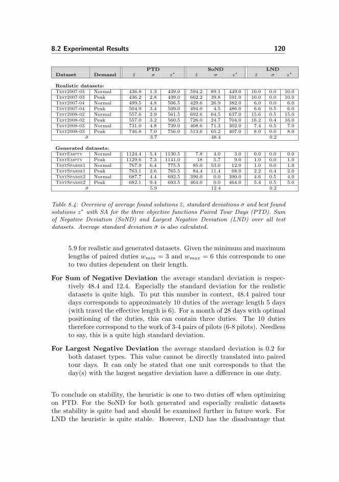
8.2 Experimental Results 120
PTD SoND LNDDataset Demand z σ z∗ z σ z∗ z σ z∗
Realistic datasets:Test2007-03 Normal 436.8 1.3 439.0 594.2 89.1 449.0 10.0 0.0 10.0Test2007-03 Peak 436.2 2.8 439.0 662.2 39.8 591.0 10.0 0.0 10.0Test2007-04 Normal 499.5 4.8 506.5 429.6 26.9 382.0 6.0 0.0 6.0Test2007-04 Peak 504.9 3.4 509.0 494.0 4.5 486.0 6.6 0.5 6.0Test2008-02 Normal 557.6 2.9 561.5 692.6 64.5 637.0 15.6 0.5 15.0Test2008-02 Peak 557.0 3.2 560.5 726.0 24.7 704.0 16.2 0.4 16.0Test2008-03 Normal 731.0 4.8 739.0 408.6 71.3 302.0 7.4 0.5 7.0Test2008-03 Peak 746.8 7.0 756.0 513.6 65.2 407.0 8.0 0.0 8.0
σ 3.7 48.4 0.2
Generated datasets:TestEmpty Normal 1124.4 5.4 1130.5 7.8 4.0 3.0 0.0 0.0 0.0TestEmpty Peak 1129.6 7.3 1141.0 18 5.7 9.0 1.0 0.0 1.0TestSparse1 Normal 767.9 6.4 775.5 85.0 53.0 12.0 1.0 0.0 1.0TestSparse1 Peak 763.1 2.6 765.5 84.4 11.4 68.0 2.2 0.4 2.0TestSparse2 Normal 687.7 4.4 692.5 390.0 0.0 390.0 4.6 0.5 4.0TestSparse2 Peak 682.1 9.4 693.5 464.0 0.0 464.0 5.4 0.5 5.0
σ 5.9 12.4 0.2
Table 8.4: Overview of average found solutions z, standard deviations σ and best foundsolutions z∗ with SA for the three objective functions Paired Tour Days (PTD). Sumof Negative Deviation (SoND) and Largest Negative Deviation (LND) over all testdatasets. Average standard deviation σ is also calculated.
5.9 for realistic and generated datasets. Given the minimum and maximumlengths of paired duties wmin = 3 and wmax = 6 this corresponds to oneto two duties dependent on their length.
For Sum of Negative Deviation the average standard deviation is respec-tively 48.4 and 12.4. Especially the standard deviation for the realisticdatasets is quite high. To put this number in context, 48.4 paired tourdays corresponds to approximately 10 duties of the average length 5 days(with travel the effective length is 6). For a month of 28 days with optimalpositioning of the duties, this can contain three duties. The 10 dutiestherefore correspond to the work of 3-4 pairs of pilots (6-8 pilots). Needlessto say, this is a quite high standard deviation.
For Largest Negative Deviation the average standard deviation is 0.2 forboth dataset types. This value cannot be directly translated into pairedtour days. It can only be stated that one unit corresponds to that theday(s) with the largest negative deviation have a difference in one duty.
To conclude on stability, the heuristic is one to two duties off when optimizingon PTD. For the SoND for both generated and especially realistic datasetsthe stability is quite bad and should be examined further in future work. ForLND the heuristic is quite stable. However, LND has the disadvantage that

8.2 Experimental Results 121
information on the largest negative deviation does not provide anything on theprofile of the solution. It should be noted that following section 4.3.1.4 and thetuning process, we have attempted to find the parameter settings that providethe best results as the main priority with stability with a lower priority. Alteringthese priorities could of course render results with different properties than seenin this section.
8.2.2.2 Conclusion on Testing
The testing has given two subjects to conclude on; solution values and solutionstability. The solutions found are generally quite far from the bounds given.For stability it has been shown that for objective functions PTD and LND thestability is relatively good. For SoND the stability is not very good, furtherwork should be done on finding out why this is.
We will not go into further detail with the Simulated Annealing. It will howeverbe used as an embedded part of a larger framework to find better solutions inthe next chapter.

Chapter 9
Column Matheuristic - AMatheuristic Approach to
Column Generation
In this section we will go through an approach inspired by Column Generation.As we will see, this approach shows some difficulties with regards to properlydefining the Column Generation Sub Problem (CGSP). In order to overcomethis obstacle, we have developed a solution method that combines the MasterProblem from the original Column Generation approach with a new SubProblem scheme, using the Simulated Annealing described in chapter 8. Sucha method, that is a hybrid between an exact method and a heuristic is calleda Matheuristic1 (or hybrid heuristic). We will refer to our solution approach asColumn Matheuristic.
9.1 Introduction
In this section we will give a brief introduction to the concept of ColumnGeneration as well as Matheuristics.
1Intentionally spelled Matheuristic with only one “h”

9.1 Introduction 123
9.1.1 Column Generation Theory
Column generation is a solution method for solving large linear programs. AColumn Generation based solution approach has two levels. On the first levela linear problem called the Master Problem is defined. The Master Problemcan be regarded as the original problem, but with only a subset of the variablesconsidered. On the second level is the Sub Problem. The Sub Problem can beregarded as a column generator where a column corresponds to the informationon a variable. In figure 9.1 an overview of the inter action between the Masterand the Sub Problem is illustrated. In the following we will describe how theColumn Generation method works.
Figure 9.1: The interaction between the Master and Sub Problem is illustrated. Dualvalues are produced when solving the restricted Master Problem. These are used inthe Sub Problem to find promising columns to introduce in the Master Problem. Thecolumns are transmitted back to the Master Problem, which is then resolved. Thiscontinues until no dual values values provide information to generate new columns.
Let the following linear program be the Master Problem. It could also be aninteger program.
min.:∑j∈J
cj · λj (9.1a)
st.:∑j∈J
aj · λj ≥ b (9.1b)
λj ≥ 0 ∀j ∈ J (9.1c)
In this model λj are variables representing the columns. cj is the cost of columnj and aj and b defines the constraints of the model. When having access toa feasible solution, we then have a vector of dual values associated with thecurrent basis. These dual values can be used for finding non-basis columns thatwould potentially improve the solution. However, because of the typically largesize of the linear programs and hence the large number of columns, inspectionof all non-basis columns could be an impossible task. Therefore columns are

9.1 Introduction 124
generated as they are needed. The Master Problem is then called a RestrictedMaster Problem.
The Restricted Master Problem is solved to optimality and λ and π are theprimal and dual optimal solutions. The Sub Problem now consists of findingcolumn(s) that maximizes the term (cj−πt ·aj) among the columns that are notin basis, if the problem at hand is a maximization problem. The minimum isdesired if the problem is a minimization problem. The column(s) are transmittedback to the Restricted Master Problem. If there are no columns for which(cj − πt · aj) > 0 the optimal solution to the Restricted Master Problem isalso the optimal solution to the Master Problem. If column(s) are found theprocedure is repeated iteratively. Returning to figure 9.1, one iteration of theColumn Generation solution procedure is shown.
9.1.2 Matheuristic Theory
Available techniques for solving hard combinatorial optimization problems canbe classified into two categories, exact and heuristic methods. In this thesiswe have looked at both types of methods. As we saw exact methods cannotalways be used for solving large or real instances of a hard combinatorialproblem, and can sometimes be very time consuming when solving even smallinstances. Heuristic methods can then sometimes be successfully applied. Oneof the advantages of a heuristic method is the low time consumption. Solutionscan usually be found fairly quick. However, optimal solution values are notguaranteed and the heuristic can sometimes be far of. The optimality of thefound solution is traded for a better run time.
Matheuristics are also called hybrid metaheuristics. The word hybrid meanssomething of mixed origin or composition. A Matheuristic is a combination ofan exact method and a heuristic method. (Puchinger and Raidl, 2005) cate-gorize the Matheuristics into two sub groups, Collaborative Combinations andIntegrative Combinations. In a Collaborative Combination the exact methodand the heuristic method exchange information, but are not incorporated intoeach other. An Integrated Combination implies that one method is embeddedin the other. The literature we have been able to find on the area of combiningexact and heuristic methods is fairly recent. Surveys of the area are givenin (Puchinger and Raidl, 2005) and (Raidl, 2006). A recent article, (Espinozaet al., 2008b), solves a Dial-a-Flight Scheduling Problem using a Matheuristicwhich is a local search with an incorporated optimization core.
We will use an Integrative Combination of Integer Programming and a modifiedversion of our Simulated Annealing, which is presented in chapter 8.

9.2 Master Problem 125
First we will describe the Master Problem of this approach. Next in section 9.3we will go through the Sub Problem in the Column Generation method, andthere after describe the new Sub Problem that makes use of the simulatedannealing heuristic. In section 9.5 we will describe how the Master Problemand the heuristic Sub Problem interact. We will further describe how columnsare managed and other issues related to the function of the algorithm. Wewill describe the tuning of the Matheuristic in section 9.6.1 and with the foundoptimal settings we will test the performance in section 9.6.2 and report ourfindings.
9.2 Master Problem
Except for the rules we in section 4.2.3 decided to omit, ([R8] and [R10]), allrules stated in section 3.3 are implemented in this method.
A single column is defined as a paired duty, either a single or a double. There aretwo pilots in a single duty and three pilots in a double duty. In other words, for apaired duty, a single column contains the information that master pilot A pairswith subordinate pilot B starting on day jA = jB with duty length lA = lB .For a column representing a double duty , the column contains information onthe master pilot A that is consistent throughout the double duty, the startingday j and length lA of the double duty. Further more the column containsinformation on the first subordinate pilot B in the double duty, his starting dayjB and length lB of his part of the duty. Likewise for the second subordinatepilot C, information on the starting day jC and length lC is associated with thecolumn.
A roster for a pilot consists of a number of columns depending on the numberof duties he is assigned to in the solution.
The structure of the columns and an Exclusion Matrix cover most of the rulesin the problem. In the following we will describe which columns are feasibleand hence created and how an Exclusion Matrix handles rules that cannot becovered during the column construction phase.
The restrictions on the rosters, stated in section 3.3, are ensured with the meansof different methods. As we will see later when stating the mathematical modelof the Master Problem, some restrictions are represented in the model usingconstraints. However a subset of the rules in the problem can be handled whencreating the columns.
9.2 Master Problem 126
The rules [R2] and [R3] regarding duration of a duty can be included simply bynot creating columns representing paired duties that violate these rules. Henceonly columns with duty lengths Lp = {wmin, . . . , wmax} are created.
In the construction of the columns only feasible columns with regards to pairsof pilots are allowed. That is, a paired duty can only be created if the concernedpilots are compatible according to rule [R9]. No columns are created for pairsconsisting of two low-timer pilots or two first-officers.
By taking advantage of the Availability Matrix described in section 4.4.2 we canlocate the feasible periods to assign a duty for any given pilot. To refresh, theAvailability Matrix indicates where a pilot is available for work, while takingrequired buffer into consideration. Keeping the legal pairs of pilots in mind,we are then able to locate periods where two pilots together can be assigned toa paired duty. If two pilots can work in the same time period for a minimumof wmin consecutive days they are “compatible”. In other words, for a givenduty, two pilots are compatible if the assignment of the duty in question doesnot conflict with pre-assignments and their buffers. By using the informationlocated in the Availability Matrix we can ensure that all consecutive days-off(buffers) in connection with an pre-assignment is respected (rule [R1]). Howeverthe buffer for duties assigned in a solution cannot be handled in the generationof the columns. For the purpose of ensuring that rule [R1] is not violated in theprocess of assigning duties, an Exclusion Matrix is created. We will return tothis later in this section when introducing the model of the Master Problem.
Rule [R4] regarding length of individual events is relevant for double dutycolumns and columns that are located in connection to a pre-assignment.However, the task of identifying the possible duties to generate as columnsis no different that for regular duties. The Availability Matrix can provide therequired information as to where a duty can be assigned in connection with apre-assignment. For double duties only columns with length Lp ≥ wmin for bothsubordinate pilots are created. Thus, only columns that do not violate rule [R4]is created.
The fact that all duties must begin and end with half a day of traveling has noinfluence on the duties and the columns created. However we must ensure thatthe travel periods are not included when registering the fulfillment of demandand when counting the number of paired tour days in a solution.
This concludes the rules we are able to include in the creation of the columns.The rules we have yet not included are the rules regarding work limits [R5] and[R6] and rule [R1] with regards to duties assigned in the planning process. Theserules are ensured by constraints in the model of the Master Problem. For oneof these constraints we employ the Exclusion Matrix mentioned earlier.

9.2 Master Problem 127
The structure of the columns entails, that the selection of a given column mustexclude any other columns with any of the pilots involved, that do not have aproper buffer distance (days-off); e.g. conflicting columns by rule [R1]. For thispurpose an Exclusion Matrix is constructed stating which columns that cannotbe selected in the case the column in question is selected. Two columns conflictif the columns share a pilot and the duties in the columns are located in thesame or part of the same time units. Additionally columns conflict, when theyshare one or two pilots where one duty overlaps the buffer time needed prior toor after a duty. Figure 9.2 illustrates examples of conflicting columns. Case A:Two duties sharing the pilot Joe are overlapping each other in time. Case B:Two duties are located such that the required buffer is not present. Since Joeappear in both duties, these exclude each other.
Figure 9.2: Two examples of conflicting columns. In case A two duties overlap intime and share a pilot; these exclude each other. In case B the two duties also share apilot, but do not overlap. However the duties exclude each other as there are not woff
consecutive days off between the two duties. In this case columns are also conflicting.
We now introduce a variable representing each column:
xc :{
1 if column c is chosen0 otherwise
The Exclusion Matrix has the variable for each column listed both as rowsand columns. The entries of the matrix indicate whether selecting the columnrepresented by the variable in the row exclude other columns. An example ofhow an Exclusion Matrix is generated is illustrated in figure 9.3. The figureshows four duties {A,B,C,D} and how these are located in relation to eachother. On the duties it is stated which two pilots is assigned the duty. DutyA is assigned to the pilots Joe and Ben. The same two pilots have a potentialduty B five days after the end of duty A. This is legal as no rules are violated,hence these columns representing the duties do not exclude each other. This isillustrated in the Exclusion Matrix E of the problem. Duty A excludes duty Cdue to the fact that Joe cannot be part of both duties as the overlap in time.Duty D is not excluded by any of the other duties and hence does not excludeany other duties it self because the pilots is not part of any of the other duties.No columns exclude them selves, illustrated by the 0 values in the diagonal.
The exclusion of columns is performed on a pilot level and not on duty level.

9.2 Master Problem 128
Figure 9.3: An example of how the Exclusion Matrix is constructed. There are fourdifferent duties. The columns excluded can be identified by looking at the ExclusionMatrix.
Thus when registering the exclusion of other columns with regards to a doubleduty, the two subordinate pilots here have separate exclusion patterns. Thebuffer is calculated from the individual duties of each pilot. Figure 9.4 illustrateshow the buffer is registered in a double duty. At the right, case B, it is illustratedwhy we need to create the sets of excluded columns for each column on a pilotlevel. In a double duty the buffers for each pilot differ. If the buffers are notcalculated for each pilot in the duty, other columns will be incorrectly excluded.
Figure 9.4: The calculation of buffer is performed on pilot level so other columns arenot wrongly excluded because of wrong buffer calculations. Case A show the per pilotlevel; case B per longest duty. We use the per pilot level.
As can be seen the matrix is symmetric, which can be explained by the fact that

9.2 Master Problem 129
exclusion of columns are mutual. However if one column excludes five columnsit does not automatically imply that these five columns exclude each other.Specific details on how the Exclusion Matrix is implemented and updated canbe found in section 9.5.2.1.
We will now move on to the model of the Master Problem. A solution to theproblem consists of a selection of columns with regard to the constraints inthe model. The zero-solution is also possible (and feasible), this just denotea solution where no pilots are working (except for their pre-assignments). Asolution can vary in size. The number of columns in a solution equals thenumber of duties in the solution.
As mentioned above, most of the modeling of various rules from the originalproblem is transferred into the generation of the Exclusion Matrix and into thegeneration of the feasible columns. Therefore the following model only containconstraints ensuring that maximum working day limits are respected for eachpilot, rule [R4] and [R5]. As for the other solution methods presented we hereuse the PTD objective function.
The variables stated earlier in the section are used in the model, to recall:
xc :{
1 if column c is chosen0 otherwise
The following sets are used:
P PilotsJ DaysT Time periodsC ColumnsCp Columns involving pilot p, Cp ⊂ CEc All columns excluded by c, Ec ⊂ C
Parameters in the model:
Mc = |Ec| No. of columns excluded by any of the two pilots in the pair of column cLc,p No. of work days in column c for pilot pWp Maximum no. of work days available for pilot pPTc Number of paired tour days in column c

9.2 Master Problem 130
max.:∑c∈C
PTc · xc (9.2a)∑c∈Cp
Lc,p · xc ≤Wp ∀p ∈ P (9.2b)
∑c∗∈Ec
xc∗ ≤ (1− xc) ·Mc ∀c ∈ C (9.2c)
xc = {0, 1} (9.2d)
(9.2b) constrains the pilot to not work more than their maximum allowed days.This is done for all pilots. The length of the column and hence the duty isincluded in the sum if it is chosen, indicated by the binary variable. Thissum cannot exceed Wp. Wp is calculated in the Availability Matrix, and wasalso described in section 4.5 in equation (4.8). It is the number of availabledays a pilot can work, while taking the working limits and pre-assignments intoaccount.
(9.2c) manages the exclusion among columns. If the column c is selected noneof the columns that it excludes can be selected. This is managed through atight Big-M notation. Ec is the set of columns excluded by column c. The setof columns correspond to the entries with the value 1 in the row representingthe column c. The constant Mc is set to the number of columns excluded bycolumn c, i.e. Mc = |Ec|. If column c is chosen the variable xc assumes thevalue 1 and the term (1−xc) on the right hand side of the equation becomes 0.This forces the left hand side to become 0, i.e. no columns excluded by columnc can be chosen. If column c is no chosen the term (1 − xc) is 1 and the righthand therefore totals to Mc. This allows the left hand side to be at most Mc,which allow all columns excluded by c to be chosen. Since this is done for eachcolumn c no columns that exclude each other can appear in the same solution.
9.2.1 Problem Size
The model stated have two different types of constraints. There is one constraintfor every pilot in the problem ensuring the workday limits, equation (9.2b).There are as many exclusion constraints, equation (9.2c) as there are columnsincluded in the Master Problem.
In the model there is one variable for each column included in the problem.Table 9.1 summarizes the size of the model. The fact that the number ofconstraints grows according to the amount of columns included in the problem,imply that we can only include a subset of all possible columns when solving

9.3 Column Generation Sub Problem 131
Constraints NumberWork limits (9.2b) |P |Exclusion (9.2c) |C|
Variables Numberxc |C|
Table 9.1: The size of the model in the Master Problem. There are one binary variablefor each column included. There are |C| + |P | constraints in the problem, i.e. thenumber of columns include plus the number of pilots in the problem instance.
a problem. The fraction of the columns included and hence the fraction of allpossible duties, of course depends on the size and structure of the problem.The Master Problem will now be referred to as the Restricted Master Problem(RMP).
9.3 Column Generation Sub Problem
We have now formulated the RMP and now wish to find a way to identify goodcolumns to introduce in the RMP. In the beginning of the chapter we saw howthis procedure is usually done. The dual values are used in the Sub Problemfor determining the columns to introduce in the RMP. However as we shall seein this section we are not able to use the information from the dual values. Wewill in this section go through the problems we experienced when attempting tomake use of the dual variables.
We wish to find promising columns to introduce in order to improve the solutionas much as possible. By identifying the areas where the least demand is fulfilledwe get information on where in the planning period it would be beneficial toassign a duty.
There are dual values associated with all constraints in the model. The dualvalues for the constraints in equation (9.2b) indicates what can be gained byletting the pilot in the constraint work one day more than the limits allow.This information could be useful as a decision support tool. Often the rulesand regulations are not strict and can be violated. For example a pilot can bepayed overtime for the time he exceeds the work limits. However the informationprovided by the dual variables of equation (9.2b) cannot be used for determiningwhich columns to introduce in order to potentially improve the solution.

9.4 Matheuristic Sub Problem 132
Dual values stemming from equation (9.2c) provide information on what canbe gained if the exclusion constraint were to be relaxed by one. In other wordswhat is the gain of allowing one of the columns c excludes to be chosen alongwith c. We cannot use this information for finding good columns to introduce.The individual exclusion of a column have no direct connection the number ofpaired tour days we are able to gain if we were able to choose the two columnsin question together. The column could easily be excluded by another columnin basis, and thus would not alter the solution found.
With this model we are left with no way of finding good columns to introduceaccording to our goal of meeting demand. In the problem we have nodifferentiation of the pilots or the duties. That is, there are no ways ofdifferentiating between possible columns to introduce. The gain of introducinga duty in one time unit is the same as introducing a duty in any other timeunit. Potentially a combination of the various dual values could be used todifferentiate, but this will still not differentiate enough for our needs.
We recall the shortage and surplus variables presented in section 4.3.1:
s+j,t, s
−j,t : ≥ 0, surplus (+) or shortage (−) on day j, time t
By introducing these to the RMP model along with equation (9.3) we haveaccess to another type of dual values.∑
c∈Cj,t
xc − s+j,t + s−j,t = demj,t ∀j ∈ J, t ∈ T (9.3)
These dual values indicate where in time we would gain the most if assigning aduty. However as mentioned we are not able to differentiate between columns,thus all dual variables from (9.3) assume identical values. This gives rise toanother definition of the Sub Problem, where no dual variables are applied.
9.4 Matheuristic Sub Problem
We now move on to defining the Column Matheuristic Sub Problem (CMHSP).We saw in the previous section that using the dual variables to price the non-basis columns is not possible. We therefore do not use these and instead willlook at other ways of finding good columns to introduce in the RMP.
The variables s+j,t and s−j,t introduced in the previous section can serve another
purpose. We are able to use the variables to determine which columns tointroduce in the RMP, or at least narrow down the search. The s−j,t values

9.4 Matheuristic Sub Problem 133
provide information on how much the solution differs from the demand on thegiven day and time period. We have access to this information for all days andall time periods. However since the duties we can introduce in the columns areat least wmin days long, looking at one time unit separately does not providethe desired information. By looking at minimum 6 time units corresponding to3 full days at once we are able to calculate what we refer to as the desired requestarea. This area indicates where it is most beneficial with regards to deviationfrom demand to assign a duty, i.e. what columns to introduce with regards tothe time location. The desired request area is calculated as the area that hasthe largest sum of the s−j,t variables of all possible areas in the planning period.The length of the area is fixed when locating the desired request area.
Figure 9.5: The desired request area is found as the area of length wmin with the largestsum of deviation from demand s−j,t in the time units.
Figure 9.5 illustrates how the desired request area is found. Five request areasare calculated and the area with the largest sum of s−j,t variables is the desiredrequest area. This is the area in the planning period that is in most need ofduties and hence columns.
There are different ways of defining the requested area. The length of a dutyis between wmin and wmax days. Hence areas of the same length will makesense to apply. Areas of length greater than wmax cannot be covered by a dutyand could might as well be of length wmax. The shortest duty we are able tointroduce is of length wmin and hence we might as well include information onthe areas of this minimum length.
There are also decisions regarding how much of the area to cover by the columns.Only columns that cover the area fully could be allowed to be introduced, orcolumns covering some fraction of the area could also be allowed.

9.4 Matheuristic Sub Problem 134
We have chosen to work with an area that as length wmin and only allow theintroduction of columns that fully cover the area. It should be mentioned thatthe area we have chosen to work with actually only covers 4 time units whichcorresponds to a duty of length wmin as the two travel periods in the beginningand end of the duty do not fulfill demand. However, for simplicity, we willconsider the duties in full length. For a given request area of length wminfigure 9.6 illustrates which column/duties are included in the pool of potentialcolumns to introduce.
Figure 9.6: For a given request area the column candidates to introduce in the RMPare illustrated. All duties cover the area fully.
At this point we again experience trouble with the differentiation of columns. Wehave found an area where introducing columns are most needed with regards tothe fulfillment of demand. And with the assumption that only columns coveringthe area fully we have identified potential columns to introduce.
The issue of choosing which pairs of pilots to introduce arises. Because thereis a huge amount of possible pairs and no distinction between the pairs, thenumber of columns to introduce can potentially be very large. As it is onlypossible to include a limited amount of columns we are forced to choose betweenthe equally qualified candidate columns. This means that a certain level ofstochastic behavior is required when choosing the columns to introduce in theRMP. We have no way of distinguishing between the equally qualified columnsin the candidate pool.
We can use the Simulated Annealing heuristic described in chapter 8 to generatecolumns that cover the desired request area. By modifying the SA we cangenerate solutions containing only duties that cover the desired requested area,like the valid duties shown in figure 9.6. The generated solution from the SAcan then be transformed into a number of columns corresponding to the number

9.5 The Column Matheuristic 135
of duties in the solution.
The solution generated for the desired request area is a legal solution, that is allrules are respected. Hence no columns excluding each other is included. For thisreason the number of columns resulting from one solution to the area is limited.However if a larger number of columns to introduce in the RMP is desired, theSA is run multiple times until the desired number of columns is reached. Inthe first run all columns are included in the pool of columns to introduce inthe RMP. The columns resulting from the runs of SA are only included in thepool of columns to introduce if they are distinct, i.e. if the same column is notalready in the pool.
We have now described how we have chosen to modify the regular CGSPinto a Sub Problem that utilizes of the implementation of the SimulatedAnnealing heuristic. In the next section we will describe how the RMP andthe Matheuristic Sub Problem are connected and how they interact.
9.5 The Column Matheuristic
In this section we will describe how the RMP and the Column Matheuristic SubProblem, CMHSP, work together. We will start by describing one iteration ofthe method and then move on to how the CMH operates across several iterationsin section 9.5.3.
Figure 9.7: Schematic representation of the Column Matheuristic (CMH).
Figure 9.7 is a schematic representation of how the Column MatheuristicCMH functions. The CMH has the possibility of getting a “kick start” inthe form of warmstarts. The RMP is then solved and the current solution is

9.5 The Column Matheuristic 136
transmitted to the CMHSP which then calculates the desired request area. Withthe information on the location of the desired request area valid columns aregenerated in the CMHSP. If there are more columns than the RMP is capableof handling, some of the columns that are not in basis are deleted according toa Column Management Scheme, which we will describe later. The generatedcolumns are then transferred back to the RMP. This is done iteratively untilstopping a criteria is reached. The final solution is then the last and best foundsolution of the RMP. In the following we will go through the different steps inthe algorithm in more detail and discuss how they are executed. We start bydescribing the possibility of “kick starting” the algorithm with warmstarts.
9.5.1 Description of the Warmstart Procedure
With the Simulated Annealing heuristic we are able to produce a number ofdifferent solutions for a dataset. These solutions can be transformed intocolumns which are then transferred to the RMP. Depending on the ColumnScheme for introducing columns either a large amount of columns in one singlerequest area is introduced in one iteration or a smaller preset amount of columns.Many iterations are needed in order to achieve a set of duties covering all daysif warmstarts are not applied. In the first iteration of the algorithm all dayswill then very likely be covered. We will discuss further in section 9.5.2 whichColumn Management Scheme we have chosen to follow.
If several warmstarts are used only distinct columns are included in the pool ofcolumns to introduce in the RMP. That is, if two or more warmstart solutionshave the same column included, only one of these will be transferred in to theRMP. We have chosen to “kick start” the algorithm in our implementation. Thetime used for generating a single warmstart solution is the same as the time usedby the SA in the CMHSP when generating new columns to introduce.
After the generated warmstarts have ended, the solutions from these aretransformed into columns that are transferred into the RMP. Only distinctcolumns are included. The RMP is then solved with the columns from thewarmstart.
When the optimal solution is found in the current RMP, the solution informationis transferred to the CMHSP. On the basis of the current solution the desiredrequest area is found. Columns are then generated using the SA. There areseveral different schemes to follow when determining the number of distinctcolumns to generate and introduce in the RMP. Schemes clarifying how to handlecolumns are called Column Management Schemes. In the following we willdescribe the column management scheme we have applied.
9.5 The Column Matheuristic 137
9.5.2 Column Management Schemes in the RMP andCMHSP
The decisions of how many columns to introduce to the RMP in each iteration,and if any columns that are not in basis, should be deleted to make room for newcolumns are all column management issues. Column Management Schemes hasthe objective of controlling the size of the active RMP as we can only includea limited amount of columns in each RMP. The (Savelsbergh and Sol, 1998)describes several Column Management Schemes.
The first decision to make is how many columns to introduce. The number ofcolumns introduced along with the number of columns deleted determine the sizeof the RMP. We could potentially only introduce one column at a time. Howeverthis is not wise, as we are not capable of differentiating the columns, and wouldhave to pick one at random. We have chosen to include a predetermined amountof columns depending on the size of the column pool. We limit the columnsintroduced to maintain a somewhat equal distribution of the location of thecolumns with regards to the planning period. The generated columns are alllocated within a limited number of time units around the desired request area. Itis possible that we cannot find enough distinct columns in the desired requestedarea to reach the predetermined number of columns to introduce. In that casethe generation of columns are stopped if no new columns are found in a while.
When introducing new columns, we extract and delete approximately the sameamount of non-used columns in the column pool. These can possibly bereintroduced in later iterations. The columns we delete in a given iterationare the columns that have not been part of a solution for the largest numberof past iterations. If these are not enough, the columns that have not been inbasis the second longest time are deleted and so forth until enough columns ormore have been deleted.
When the new columns are introduced to the RMP, the model is updated toinclude the columns in the new column pool. In order to do, so the ExclusionMatrix has to be updated.
9.5.2.1 Updating the Exclusion Matrix
When the columns to introduce are found they have to be transferred backto the RMP. For these columns the individual sets Ec of other columns theindividual column exclude, are not yet created because the Exclusion MatrixE is pre-generated in a preprocessing phase for the unique column patterns in

9.5 The Column Matheuristic 138
the problem. However generating the set Ec for any given c becomes an easytask because of the preprocessing phase. The possible columns in any datasetfollow a limited number of patterns when not regarding which pilots are in theduties. On every day there are four possible duty patterns. A duty with lengthwmin = 3, one with length 4, one with length 5 and the last with length 6. Theseduties can be assigned starting each day of the planning period. Therefore wehave 4 ·ndays different unique patterns. For each pattern it is given which otherpatterns it excludes. When introducing a new column in the RMP the set Eccan be directly determined from the pattern of the column to be introduced. Inthe this way updating the RMP is easy, since it is only the pilots that need tobe considered, then patterns exclusions are already generated.
In the next section we look at how the Column Matheuristic works over severaliterations.
9.5.3 Issues Regarding Several Iterations
In the first iteration the RMP is solved with columns from numerous warmstarts.In the CMHSP new columns are generated and an amount of columns need tobe deleted in order to make room for the newly generated columns. Howeverall columns that are not in basis have never been part of any solution as onlythe current solution has been generated. Therefore all columns that are not inbasis are deleted from the column pool. Over several iterations the size of thecolumn pool follows the graph illustrated in figure 9.8. The warmstarts givea large amount of columns. In the second iteration all columns that are notin basis are deleted and a number of new columns is introduced. The numberis a predetermined fraction of the pool size limit. The pool size grows as newcolumns are introduced. No old columns are required to be deleted as thecolumn pool size limit is not reached in the next couple of iterations. When thelimit after some iterations is reached, “old” columns are again deleted.
When running multiple iterations of the algorithms another issue related to therequest area arises. If it proves difficult to meet demand in a certain area ofthe planning period, there is a possibility that this area will be found as thedesired request area in numerous consecutive iterations. If no new columns canbe found, we wish to move on to another area. To avoid “getting stuck” in suchan area a modified tabu list can be used. The tabu list have a predeterminedsize. The concept of a tabu list is described in (Gendreau and Potvin, 2005).However applying such a list has several disadvantages in connection to ourproblem. Because of the structure of our problem there is a limited number ofpossible request areas. And if a number of request areas prove impossible tofulfill, these will be registered on the tabu list. If the tabu list size is larger than

9.5 The Column Matheuristic 139
Figure 9.8: The variation of the column pool size when introducing and deletingcolumns in each iteration.
the number of impossible request areas the areas will never get of the tabu list.Since our algorithm is stochastic, the generation of columns in the areas mightnot be impossible. For this reason we would like the opportunity to return toall request areas with time. A tabu list might make this impossible.
Instead we have used a penalty list inspired by the idea behind a tabu list.Whenever an area is found to be the desired requested area and columns aregenerated, the time units in the area receives a penalty of 1. The penalty issubtracted from the lack in demand, i.e. the s−j,t variables in the given timeunits. In this way the area becomes less in need of crew. Every time a desiredrequest area is determined and columns are generated a penalty of 1 is given.In this way we are able to try the same request area several consecutive timesdepending on how much lack of the demand the area has. We are always able toreturn to a given area, as all possible areas become less attractive as well whencolumns have been generated for the areas. In figure 9.9 six iterations showingthe desired request areas illustrated by the grey boxes and the updating of thepenalty is illustrated. The negative deviation −s−j,t is illustrated in the uppergraph and the penalty on the time units below. In iteration A the area {4, 5, 6}is found. If more than one area has the largest negative deviation from demandincluding the penalty the area located earliest is chosen. The area A is thenpenalized and the negative deviation is updated. The penalty is illustrated inthe iteration. The penalty list shows it purpose especially in iteration E, whereone should think that area {1, 2, 3} would be chosen with the left-first search.But due to the penalty the area {4, 5, 6} is chosen. This behavior is also inaction in iteration F, where {7, 8, 9} is chosen due to the penalties.
We now move on to describing how the final solution is achieved. The algorithm

9.5 The Column Matheuristic 140
Figure 9.9: The effect of the penalty list. The lack according to demand is given overa six iteration period. When a area is selected (illustrated by the grey box) a penaltyof one is added to reduce the lack. If all areas are equal the earliest located area ischosen. Observe how the area {1, 2, 3} is not chosen in iteration E and F.
can in theory run an infinite amount of time. In order to make sure the optimalsolution is found all possible combinations of columns have to be investigated.The number of columns in a solution is equivalent to the number of duties in asolution. This number highly depend on the size of the problem, the days in theplanning month, the sparsity and the difficulty of the problem. A solution onthe datasets used in this thesis consists of approximately 100-200 columns andthe number of possible columns is astronomical. Therefore instead of trying toinvestigate all possible solutions we try to investigate solutions we believe to begood. For this reason a stopping criteria is needed. We have chosen to operatewith a time limit stopping criteria.
In the following sections we will report and discuss the results we have achievedwith the Column Matheuristic.
9.6 Experimental Results 141
9.6 Experimental Results
This section is split into two main parts, as was the experimental results for theSimulated Annealing. First the tuning of the Column Matheuristic in order tofind the best settings for the parameters and second testing and solutions withthe best parameter settings found in the tuning part.
As commented on earlier, we have decided to split our experiments with theheuristic into two parts: realistic (high ratio of pre-assignments) and generateddatasets (empty or low ratio of pre-assignments), see table 5.1. All results fromtuning and testing will be reported separately.
Experimental results have been achieved in accordance with section 4.6.Experiments have been split over several identical computers in order to decreasethe total running time for all tests. Briefly on the implementation of theCMH: The embedded SA is implemented in C# 2.0, as well as the columnpool manager. When a integer programming solution for the RMP is needed,this program call the Mosel Xpress-BCL 1.6.3 library. A description of this isgiven in appendix C.
9.6.1 Tuning of the Column Matheuristic
Initially we will have to isolate the fixed settings for the tuning phase for theColumn Matheuristic (CMH).
9.6.1.1 Settings, Parameters and Values
Settings for the CMH concern time usage: Total time pr. run, time pr.iteration of the embedded Simulated Annealing and the maximum allowed timeper iteration of solving the Integer Program containing the generated pool ofcolumns. We will set the maximal running time to 30 minutes. Preliminarytesting has shown us that this time should be enough for the algorithm tostabilize at a solution value and not improve it. Within the algorithm twocomponents are embedded: the Simulated Annealing and the Integer Programsolver.
Given that the performance and stability for the SA is already known for runsof 30 seconds (see section 8.2.2), we will choose this for the internal runs of SA.For a full running time for the Column Matheuristic, this setting will allow 60

9.6 Experimental Results 142
iterations of the Simulated Annealing not considering the solving time used forthe Integer Programs.
Secondly for the allowed time per solve of the Integer Programs we are interestedin a weigh off between optimal solutions of these against not too long runningtimes. If the IP-time is too low, optimal solutions will potentially not be found;if set to high, the time available for runs of the SA to generate new columnswill be low. The maximum allowed time for solving the Integer Programs is ofcourse only applicable when the column pool reaches a certain size. We chooseto set this maximum allowed time per solve of the IP to 4 minutes. This willallow 7-8 solving iterations of the Integer Programs not considering the timeused for the Simulated Annealing.
Given that the CMH builds on top of the Simulated Annealing heuristic it isstochastic and could potentially find a different solution value every time it isrun with the same setting on the same dataset. As previously we choose asample size of 5 in order to both get fairly trustworthy statistic results whilekeeping the running time down.
Table 9.2 summarizes the fixed settings derived by the above discussions, thatwill be used in the parameter tuning of the CMH.
Setting ValueTime per run ttotal 30 minutesTime per run of SA tsa 30 secondsMax time per solve of IP tsolve 4 minutesSample size 5
Table 9.2: Fixed settings for parameter tuning of the Column Matheuristic.
When tuning the CMH we have decided only to tune over one parameter:Maximum allowed size of the column pool. We wish to examine the following:Is it better to have a relatively small column pool size, hence allowing optimalsolutions of the (small) IPs and relatively many iterations of SA generating newcolumns? Or is it better to have a large column pool size, with a larger solutionspace, possibly at the cost of having the solving iterations take a relatively longtime, potentially not finding the optimal solutions. This will allow relatively fewiterations of SA for generating new columns. Therefore we wish to parametertune the maximum allowed size of the column pool.
The maximum size of the column pool cmax must obey cmax ≥ 0. Secondly thesize must be at least the amount of columns necessary to represent a full solution.If set lower, a solution could not be represented fully and only the subset of itwould be selected. This second requirement depends on the problem size, a
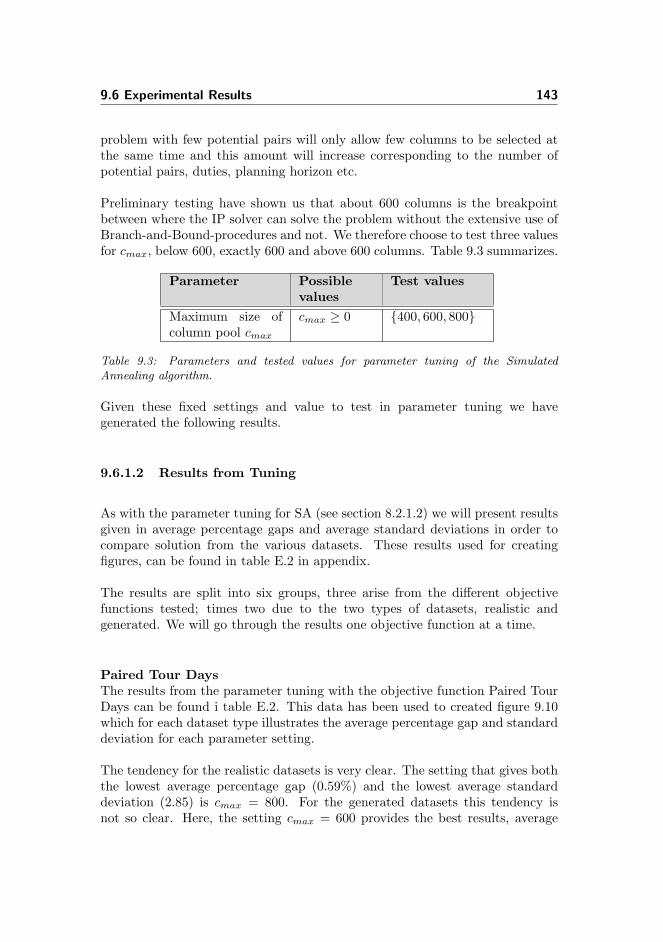
9.6 Experimental Results 143
problem with few potential pairs will only allow few columns to be selected atthe same time and this amount will increase corresponding to the number ofpotential pairs, duties, planning horizon etc.
Preliminary testing have shown us that about 600 columns is the breakpointbetween where the IP solver can solve the problem without the extensive use ofBranch-and-Bound-procedures and not. We therefore choose to test three valuesfor cmax, below 600, exactly 600 and above 600 columns. Table 9.3 summarizes.
Parameter Possiblevalues
Test values
Maximum size ofcolumn pool cmax
cmax ≥ 0 {400, 600, 800}
Table 9.3: Parameters and tested values for parameter tuning of the SimulatedAnnealing algorithm.
Given these fixed settings and value to test in parameter tuning we havegenerated the following results.
9.6.1.2 Results from Tuning
As with the parameter tuning for SA (see section 8.2.1.2) we will present resultsgiven in average percentage gaps and average standard deviations in order tocompare solution from the various datasets. These results used for creatingfigures, can be found in table E.2 in appendix.
The results are split into six groups, three arise from the different objectivefunctions tested; times two due to the two types of datasets, realistic andgenerated. We will go through the results one objective function at a time.
Paired Tour DaysThe results from the parameter tuning with the objective function Paired TourDays can be found i table E.2. This data has been used to created figure 9.10which for each dataset type illustrates the average percentage gap and standarddeviation for each parameter setting.
The tendency for the realistic datasets is very clear. The setting that gives boththe lowest average percentage gap (0.59%) and the lowest average standarddeviation (2.85) is cmax = 800. For the generated datasets this tendency isnot so clear. Here, the setting cmax = 600 provides the best results, average
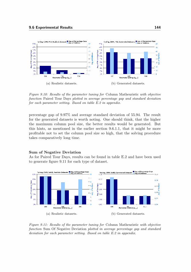
9.6 Experimental Results 144
(a) Realistic datasets. (b) Generated datasets.
Figure 9.10: Results of the parameter tuning for Column Matheuristic with objectivefunction Paired Tour Days plotted in average percentage gap and standard deviationfor each parameter setting. Based on table E.2 in appendix.
percentage gap of 9.97% and average standard deviation of 55.94. The resultfor the generated datasets is worth noting. One should think, that the higherthe maximum column pool size, the better results would be generated. Butthis hints, as mentioned in the earlier section 9.6.1.1, that it might be moreprofitable not to set the column pool size so high, that the solving proceduretakes comparatively long time.
Sum of Negative DeviationAs for Paired Tour Days, results can be found in table E.2 and have been usedto generate figure 9.11 for each type of dataset.
(a) Realistic datasets. (b) Generated datasets.
Figure 9.11: Results of the parameter tuning for Column Matheuristic with objectivefunction Sum Of Negative Deviation plotted in average percentage gap and standarddeviation for each parameter setting. Based on table E.2 in appendix.

9.6 Experimental Results 145
For the realistic datasets, the best setting is again cmax = 800. The best averagepercentage gap is chosen first (8.56%), and average standard deviation second(6.67). Actually the average standard deviation for the cmax = 600 is marginallybetter, but not enough to change the choice of setting. For the generateddatasets both settings cmax = 600 and 800 give the exact same results (0.03in average of averages and 0.07 in average standard deviation). We decide topostpone this choice of setting for the two identical results until we have theresults for the final objective function, Largest Negative Deviation.
Largest Negative DeviationAgain results can be found in table E.2 and have been used to generatefigure 9.12 for each type of dataset.
(a) Realistic datasets. (b) Generated datasets.
Figure 9.12: Results of the parameter tuning for Column Matheuristic with objectivefunction Largest Negative Deviation plotted in average percentage gap and standarddeviation for each parameter setting. Based on table E.2 in appendix.
The tendency for the realistic datasets is as for the two other objective functions,cmax = 800 is chosen. For the generated datasets, again the best results areobtained by using the middle value for the maximum column pool size, cmax =600.
9.6.1.3 Conclusion on Tuning
The table 9.4 shows the found settings from the parameter tuning. The bestsolution values, standard deviation and average solutions found with from thesamples with the selected parameter settings and used for calculating the averagepercentage gaps can be found in table E.1. To return to the selection for SoNDfor generated datasets, we choose 600 based on the fact that we for the tworemaining objective functions found this setting to be the best.

9.6 Experimental Results 146
Obj. func. Datasets cmax
PTD Realistic 800PTD Generated 600SoND Realistic 800SoND Generated 600LND Realistic 800LND Generated 600
Table 9.4: Found settings from parameter tuning of Column Matheuristic.
As with the Simulated Annealing, it would be interesting to examine if it waspossible to choose one setting for all. It can be seen that the dataset typeshave each their common setting. Examination of the results show that the bestsetting in this scenario would be to select cmax = 800. Only for LND withgenerated datasets this would be a very bad choice – for the other objectivefunctions and dataset types, cmax = 800 provides the best or almost the bestresults. However we will choose cmax = 800 for realistic datasets and cmax = 600for generated datasets for further work in this thesis.
9.6.2 Testing
We have now found the optimal parameter setting for the maximum columnpool size. In this section we test how well the Column Matheuristic performs onseveral testing datasets, this with the optimal parameter settings set. Solutionvalues and stability will be examined. Even though the Column Matheuristicembeds the Simulated Annealing, we will not discuss how the CMH improveson the solutions found by the SA, we will leave this for the upcoming chapter 10where we compare all solution approaches in this thesis. This section will endwith a minor conclusion.
9.6.2.1 Results
Tests have with the SA been run on the testing datasets from table 5.1. Settingshave been as for tuning, see table 9.2. The upcoming table 9.5 displays foreach testing dataset the average found solution z, standard deviation σ andbest found solution z∗ within each objective function together with the averagestandard deviation σ within each dataset type.
We will now comment on these results from table 9.5 listed by the objective

9.6 Experimental Results 147
PTD SoND LNDDataset Demand z σ z∗ z σ z∗ z σ z∗
Realistic datasets:Test2007-03 Normal 479.2 3.0 489.0 357.7 13.5 344.0 9.0 0.0 9.0Test2007-03 Peak 480.2 4.0 484.5 388.3 11.5 377.0 9.0 0.0 9.0Test2007-04 Normal 552.3 1.6 553.5 202.3 10.1 193.0 4.3 0.6 4.0Test2007-04 Peak 551.8 0.6 552.5 233.7 13.3 225.0 5.3 0.6 5.0Test2008-02 Normal 610.5 1.8 612.0 525.0 4.6 521.0 13.7 0.6 13.0Test2008-02 Peak 611.8 0.6 612.5 580.3 5.7 574.0 14.0 0.0 14.0Test2008-03 Normal 796.7 3.2 799.0 180.0 11.3 173.0 6.0 0.0 6.0Test2008-03 Peak 805.3 4.9 811.0 237.0 10.8 228.0 6.0 0.0 6.0
σ 2.5 10.1 0.2
Generated datasets:TestEmpty Normal 1150.8 5.3 1155.5 0.0 0.0 0.0 0.0 0.0 0.0TestEmpty Peak 1148.3 10.9 1156.5 0.0 0.0 0.0 0.7 0.6 0.0TestSparse1 Normal 793.8 7.7 802.5 0.0 0.0 0.0 1.0 0.0 1.0TestSparse1 Peak 805.8 2.6 808.0 9.7 6.7 4.0 2.7 0.6 2.0TestSparse2 Normal 718.5 2.6 721.5 344.7 12.6 333.0 4.0 0.0 4.0TestSparse2 Peak 719.0 1.8 721.0 371.7 31.9 335.0 4.0 0.0 4.0
σ 5.1 8.5 0.2
Table 9.5: Overview of average found solutions z, standard deviations σ and best foundsolutions z∗ with CMH for the three objective functions Paired Tour Days (PTD).Sum of Negative Deviation (SoND) and Largest Negative Deviation (LND) over alltest datasets. Average standard deviation σ is also calculated.
functions. As with the SA it is interesting to note that there actually is adifference in solution value for the normal demand datasets in comparison withthe peak demand datasets. We believe that this is a direct consequence of thebehavior of the SA, given that the CMH does not contain any other stochasticelements other than the SA.
For Paired Tour Days the average standard deviation is respectively 2.5 and5.1 for realistic and generated datasets. This corresponds to approximatelyone to two duties given the minimum and maximum lengths of pairedduties, wmin = 3 and wmax = 6.
For Sum of Negative Deviation the average standard deviation is respec-tively 10.1 and 8.5. This corresponds to approximately three to fourduties. It should be mentioned that the average standard deviation for thegenerated datasets is biased. For the empty dataset and for TestSparse1with normal demand the optimal solution was found every time (for SoNDthe value 0 will always be the optimal solution). For the remaining, theTestSparse1 with peak demand and both TestSparse2 datasets it wasnot possible to find the optimal. This of course influences on the averagestandard deviation which for the three latter datasets isolated would becalculated to 17.1. This corresponds to approximately six duties.

9.6 Experimental Results 148
For Largest Negative Deviation the average standard deviation is 0.2 inboth realistic and generated dataset. It is not possible to directly translatethis value into a value in paired tour days, given that this information isnot available directly.
In a brief conclusion on stability, it can be said that the CMH is one to two dutiesoff when optimizing over the objective function PTD. For SoND the stability isa little bit worse, here the CMH is three to four duties off. However, observethat the results for the generated datasets are quite biased for the SoND. Finallyfor the LND, the solution is quite stable.
9.6.2.2 Conclusion on Testing
The testing provided two results. It was shown that depending on the objectivefunction the CMH was quite stable, especially for the objective functions PTDand LND. As for the Simulated Annealing, the stability for the last objectivefunction SoND should in future work be examined further. The solutions foundare generally quite far from the bounds given.
The CMH has now been tuned and tested. In the upcoming chapter, we willcompare all solution approaches against each other. Furthermore during thiscomparison we will see how the CMH has improved on the embedded SimulatedAnnealing, which had worse stability and results than for the CMH.

Chapter 10
Comparison of SolutionApproaches
In this thesis we have introduced, modeled, implemented, tuned and testeddifferent solution approaches. To evaluate on this work, we will compare thefour solution methods and give an estimation of each methods potential use ifput into practice.
Page Solution Approach Exact Solvable?∗
62 Binary Integer Problem Yes 1 CP, 1 FO76 Multi-Commodity
Network Flow ProblemYes 3 CP, 3 FO
100 Simulated Annealing No All tested122 Column Matheuristic No All tested
Table 10.1: Overview of solution approaches in this thesis. ∗: the maximum problemsizes of 30 days and 2 time periods that the solution approaches can solve.
As the two exact methods, the BIP and MCNFP are not able to solve anyproblem sizes derived from real-life problems, we see no direct use for them forplanning in their current form. In this chapter, we will therefore only considerthe two methods, that were able to solve real-life scaled problems, the SA andCMH, which we will compare.

10.1 Comparison of Simulated Annealing against Column Matheuristic 150
10.1 Comparison of Simulated Annealing againstColumn Matheuristic
The heuristic methods, Simulated Annealing and Column Matheuristic, wereboth able to solve problems of real-life scale. The SA was embedded within theCMH. In this section we will compare the results of the two methods, both withregards to scalability and solution quality. We will go through the comparisonin details for the objective function PTD, but leave out the details for objectivefunction SoND and LND, as the review would be highly repetitive.
Table 10.2 display the testing results for SA and CMH, with the average foundsolutions z, standard deviations σ and best found solutions z∗ for each dataset.Further in the third major column the improvement the CMH had over the SAis listed for both z, σ and z∗. If a entry is positive the CMH has provided betterresults than the SA, and negative denotes the opposite. Observe that while theobjective function PTD maximizes the value, it is preferable to have an averagestandard deviation as low as possible.
Objective: PTD Simulated Column CMH improves SAAnnealing Matheuristic (% improvement)
Dataset Demand z σ z∗ z σ z∗ z σ z∗
Realistic datasets:
Test2007-03 Normal 436.8 1.3 439.0 479.2 3.0 489.0 9.7% -131.2% 11.4%Test2007-03 Peak 436.2 2.8 439.0 480.2 4.0 484.5 10.1% -44.5% 10.4%Test2007-04 Normal 499.5 4.8 506.5 552.3 1.6 553.5 10.6% 66.6% 9.3%Test2007-04 Peak 504.9 3.4 509.0 551.8 0.6 552.5 9.3% 82.8% 8.5%Test2008-02 Normal 557.6 2.9 561.5 610.5 1.8 612.0 9.5% 38.8% 9.0%Test2008-02 Peak 557.0 3.2 560.5 611.8 0.6 612.5 9.8% 82.2% 9.3%Test2008-03 Normal 731.0 4.8 739.0 796.7 3.2 799.0 9.0% 33.7% 8.1%Test2008-03 Peak 746.8 7.0 756.0 805.3 4.9 811.0 7.8% 29.6% 7.3%
Averages 3.8 2.5 9.5% 19.8% 9.2%
Generated datasets:
TestEmpty Normal 1124.4 5.4 1130.5 1150.8 5.3 1155.5 2.4% 1.9% 2.2%TestEmpty Peak 1129.6 7.3 1141.0 1148.3 10.9 1156.5 1.7% -48.3% 1.4%TestSparse1 Normal 767.9 6.4 775.5 793.8 7.7 802.5 3.4% -20.2% 3.5%TestSparse1 Peak 763.1 2.6 765.5 805.8 2.6 808.0 5.6% 2.5% 5.6%TestSparse2 Normal 687.7 4.4 692.5 718.5 2.6 721.5 4.5% 39.8% 4.2%TestSparse2 Peak 682.1 9.4 693.5 719.0 1.8 721.0 5.4% 80.8% 4.0%
Averages 5.9 5.1 3.8% 9.4% 3.5%
Table 10.2: Comparison of SA and CMH for the objective function PTD. For eachsolution approach is listed the average found solutions z, standard deviations σ andbest found solution z∗. The comparison columns are the percentage improvement forthe CMH over the SA, i.e. positive numbers denotes improvement (CMH better thanSA) and the negative the opposite.
We will examine these results first for the realistic datasets and second for thegenerated datasets. For the realistic datasets the tendency of improvement insolution values is very clear, approximately 9.5% for the average solutions and9.0% for the best found solutions. For the stabibility the improvement is evenbetter, 19.8% for the CMH over the SA. However this number is quite affectedby the large differences seen for few datasets. For example for Test2007-03,

10.1 Comparison of Simulated Annealing against Column Matheuristic 151
low numbers like σ = 1.3 for SA and σ = 3.0 for CMH is a worsening of 131.8%.Generally we see a larger improvement than the average.
For the generated datasets the tendency is the same, the CMH improves onthe SA. However, this improvement is not so large, approximately 3.8% for theaverage solutions and 3.5% for the best found solutions. The improvement ofstability is also lower than for the realistic datasets, but still noticable, 9.4%.Possibly, because of the high sparsity and low level difficulty of the generateddatasets, these are easier for the SA to get good solutions on.
The same comparison has been performed for objective functions SoND andLND. These details are to be found in tables F.1 and F.2 in appendix. Fromthese and from PTD we display the following summarizing table 10.3.
Obj: PTD Obj: SoND Obj: LNDCMH improves SA CMH improves SA CMH improves SA(% improvement) (% improvement) (% improvement)z σ z∗ z σ z∗ z σ z∗
Realistic datasets:9.5% 19.8% 9.2% 42.6% 44.8% 35.8% 17.1% 47.3% 16.9%
Generated datasets:3.8% 9.4% 3.5% 70.0% 85.4% 72.8% 10.2% 57.0% 24.0%
Weighted averages (8 realistic datasets, 6 generated datasets):7.1% 15.3% 6.8% 54.3% 58.3%a 51.7% 14.4%a 51.5%a 19.6%a
Table 10.3: Summary of comparison of SA and CMH for all objective functions.For each solution approach is listed the improvement in average found solutions z,standard deviations σ and best found solutions z∗. The percentages are the percentageimprovement for the CMH over the SA, i.e. positive numbers denotes improvement(CMH better than SA). Finally a weighted average is shown (realistic datasets withweight 8 and generated with 6); a is where the weights 8-6 are not possible, whereweights are corresponding to the number of available results for each type.
The most relevant results from table 10.3 is the improvement on the averagefound solutions. This is respectively 7.1% and 14.4% for objective function PTDand LND. This is a good improvement, which either indicates that the SA ispoor at finding good solutions or that the CMH is very good at improving onthe SA. But it could just as well be a result of the CMH being able to consider alarger solution space at the same time and therefore being able to provide bettersolutions. For the objective function SoND the improvement is 54.3% which isa drastic improvement. This indicates very clearly that the SA is quite poor atfinding good solutions for this objective function, when CMH is able to improveits results that much.

10.2 Comparison of Solution Values to Bounds 152
Comparing the improvement in stability also provides interesting results. Forthe objective function PTD this is improved 15% which is considered as a fairlygood result. For SoND and LND respectively, the improvement is 58.3% and51.5%. These improvement are again quite drastic, and indicates that the SAis not very stable. However, one should keep in mind, that while parametertuning the SA, good solutions were chosen first, and stability second. If thestability had higher priority in this selection phase, the results may very wellhave been different, providing better stability for the SA. Potentially, this couldhave provided even better stability for the CMH.
10.2 Comparison of Solution Values to Bounds
Throughout this thesis we have not had any optimal values to compare outresults to and have therefore preferred to use relative measures to compare theperformance of the algorithms. However, we will in this section examine howthe average and best solution found using the CMH are compared to the boundsintroduced in section 5.4. We have chosen generally not to do this during thethesis due to the uncertainty on the bounds. As mentioned earlier it is quite hardto find a relatively tight bound. We will only perform the comparison for testingdatasets. Table 10.4 shows the results of this comparison. The calculations areonly performed for the objective functions PTD and LND, as we have no boundfor the SoND.
PTD LNDDataset Demand z z∗ zbound z z∗ z z∗ zbound z z∗
Realistic datasets:
Test2007-03 Normal 479.2 489 944.0 49.2% 48.2% 9.0 9.0 7.0 28.6% 28.6%Test2007-03 Peak 480.2 484.5 944.0 49.1% 48.7% 9.0 9.0 7.0 28.6% 28.6%Test2007-04 Normal 552.3 553.5 1079.0 48.8% 48.7% 4.3 4.0 0.0 - -Test2007-04 Peak 551.8 552.5 1057.0 47.8% 47.7% 5.3 5.0 0.0 - -Test2008-02 Normal 610.5 612 1236.0 50.6% 50.5% 13.7 13.0 12.0 14.2% 8.3%Test2008-02 Peak 611.8 612.5 1208.0 49.4% 49.3% 14.0 14.0 12.0 16.7% 16.7%Test2008-03 Normal 796.7 799.0 1689.0 52.8% 52.7% 6.0 6.0 0.0 - -Test2008-03 Peak 805.3 811.0 1655.0 51.3% 51.0% 6.0 6.0 0.0 - -
Generated datasets:
TestEmpty Normal 1150.8 1155.5 2945.0 60.9% 60.8% 0.0 0.0 0.0 - -TestEmpty Peak 1148.3 1156.5 2945.0 61.0% 60.7% 0.7 0.0 0.0 - -TestSparse1 Normal 793.8 802.5 1986.0 60.0% 59.6% 1.0 1.0 0.0 - -TestSparse1 Peak 805.8 808.0 1986.0 59.4% 59.3% 2.7 2.0 0.0 - -TestSparse2 Normal 718.5 721.5 1768.0 59.4% 59.2% 4.0 4.0 0.0 - -TestSparse2 Peak 719.0 721.0 1768.0 59.3% 59.2% 4.0 4.0 0.0 - -
Table 10.4: Comparison of average and best found solution values of testing datasetsto bounds. The percentage gaps to the bound are shown for both average and best foundsolutions.
For the objective function PTD the tendency is quite clear, the solutions areapproximately 50% from the bound for realistic datasets, with some smallfluctuations. For the generated datasets this percentage is approximately 60%.

10.3 Solution for Test2007-03/Normal Demand 153
It is noticable that the gap to the bound is very similiar within the two datasettypes. This indicates that each dataset types has its characteristic. With regardto the gaps, 50-60% is a high gap – but as mentioned in section 4.5 the boundsare not nearly tight.
For the objective function LND we see that the bound for most datasets actuallyis 0 – the optimal value for this objective function. However, we do not alwaysfind this solution. Only for two of the generated datasets we actually find bestfound solution values of 0. There are four datasets where the bound is notzero, respectively 7 and 12. As mentioned in section 4.3.1.3 a disadvantage ofLND is that if there is an area where there are many pre-assignments it will”dominate” the rest of the solution. The bound is not tight. It might not bepossible to reach it, due to the fact that required buffer cannot be included inthe calculation of the bound.
To conclude on the comparison on bounds, future work on tighter bounds shouldbe performed in order to get a better picture of how far the CMH and SA actuallyare from the optimal solution. A second result was the very characteristicgrouping with regards to gaps of the realistic and the generated datasets forPTD.
10.3 Solution for Test2007-03/Normal Demand
In this section we will look into one single solution found by the CMH forthe dataset Test2007-03 with normal demand. We have chosen this datasetbecause it is the only dataset where we have a reference solution. JeppesenSystems has provided a comparable solution with the solution value of 507 pairedtour days, see section 5.4. To see how the CMH performs on this solution wehave run it for a half hour, 1 hours, 2 hours, 3, 6, 12 and 24 hours. Due to thetime used, each run only consisted of one sample. The solution displayed in thissection was found after 1 hour. The longer runs provided no better solutions– although they actually provided other solution, just with the same objectivevalue. This again indicates how symmetric the problem is.
In figure 10.1 the profile of the best found solution for Test2007-03 with normaldemand is shown. This solution has the objective value of 489 paired tour days,e.g. the solution provided by Jeppesen Systems contains 18 more paired tourdays (an improvement of 3.68% over the 489). For the other objective function,the solution has the value 270 for SoND and 11 for LND. We are not able tocompare these values to corresponding values for the 507-solution.
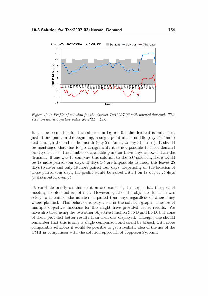
10.3 Solution for Test2007-03/Normal Demand 154
Figure 10.1: Profile of solution for the dataset Test2007-03 with normal demand. Thissolution has a objective value for PTD=489.
It can be seen, that for the solution in figure 10.1 the demand is only meetjust at one point in the beginning, a single point in the middle (day 17, “am”)and through the end of the month (day 27, “am”, to day 31, “am”). It shouldbe mentioned that due to pre-assignments it is not possible to meet demandon days 1-5, i.e. the number of available pairs on these days is lower than thedemand. If one was to compare this solution to the 507-solution, there wouldbe 18 more paired tour days. If days 1-5 are impossible to meet, this leaves 25days to cover and only 18 more paired tour days. Depending on the location ofthese paired tour days, the profile would be raised with 1 on 18 out of 25 days(if distributed evenly).
To conclude briefly on this solution one could rightly argue that the goal ofmeeting the demand is not met. However, goal of the objective function wassolely to maximize the number of paired tour days regardless of where theywhere planned. This behavior is very clear in the solution graph. The use ofmultiple objective functions for this might have provided better results. Wehave also tried using the two other objective function SoND and LND, but noneof them provided better results than then one displayed. Though, one shouldremember that this is only a single comparison and could be biased; with morecomparable solutions it would be possible to get a realistic idea of the use of theCMH in comparison with the solution approach of Jeppesen Systems.

10.4 Conclusion on Comparison 155
10.4 Conclusion on Comparison
In this section, we will conclude on the results from comparisons performed inthis chapter.
When comparing the SA with the CMH interesting tendencies arise. The CMHimproves 7.1% and 14.4% on the SA for PTD and LND. This shows that theMatheuristic approach is applicable in practice and is able to consider thesolution space in a better way than the SA, hence providing better solutions.For SoND, the improvement is so drastic, that it either indicates that the SAdoes not provide good results or that the CMH is incredibly good at improvingthe results found by the SA. For the stability, the results are even more drastic– the CMH is able to improve greatly on the SA. Generally the conclusion onthe comparison of SA to CMH, is that while further work on the SA is needed,the CMH proves its ability to improve greatly on the input it is given by SA.
The comparison of solution with bounds did not provide very much usefulinformation. More work on tighter bounds should be done in future work.However, one result was that the bounds clearly indicated that the realisticdatasets were different in characteristics than the generated datasets.

Chapter 11
Conclusion
The purpose of this thesis was to examine a specific Business Jet AirlineRostering Problem with real-life data and to investigate different modeling andsolution approaches for this.
Business Jet Airline Rostering Problems are not well described in literature dueto the fact that the underlying industry has only been around for the last 20years. Regular time-table based airlines usually split the planning process inseveral parts, for example for the crew schedule planning the problem is splitinto Pairing and Rostering phases. For the Business Jet Airline in this thesis,we have considered these as one single planning problem. This goal of theproblem is to create monthly rosters for pilots given a forecasted demand for eachday. Through assumptions and generalization we have been able to formalizethis problem in order to examine different modeling and solution approaches.Through this work, we have come up with an Availability Matrix tool, whichassists in the process of identifying where a duty for pilots potentially could beplanned. This tool serves partly as basis for our solution approaches, but couldalso be used as a self-contained decision support tool for planners.
We approached the problem with two exact methods in order to achieve insightinto the problem: First, a Binary Integer Problem (BIP) and second a Multi-Commodity Network Flow Problem (MCNFP). Both models are able to provideoptimal solutions for very small problem sizes within a short time. However, this

157
is not the case for even medium-sized problems and definitely not for problemsizes derived from real-life problems. Here, the problems cannot be solved. Weshow how the problem sizes grow drastically. The size of the MCNFP is largerthan the BIP. However, the implementation of the MCNFP is able to solve largerproblem instances than the BIP. We believe this is due to the solver being ableto pre-solve efficiently or identify structures for especially the MCNFP.
Subsequently, we implemented a heuristic approach, a Simulated Annealing(SA). The SA is able to quickly find fairly good solutions to problems of alltested sizes. However, the heuristic is not stable; the quality for each solutioncan vary greatly.
As a way of combining heuristic and exact methods, we have devised andimplemented a Matheuristic method. The idea behind is inspired by ColumnGeneration, and the method is therefore denoted Column Matheuristic (CMH )).The CMH utilizes the SA as a method for generating new columns for the exactmaster problem. The master problem is formulated in a way where columnsare greatly intertwined - when one column is chosen, it can easily rule outchoosing many other columns and vice versa. Each columns has at least oneappurtenant constraint which entails the master problem to grow with thenumber of columns. The consequence hereof is that the master problem canonly be solved up until a certain problem size (amount of columns in pool). Wehave devised a Column Management Scheme to be able to remove unprofitablecolumns from the master problem in order to keep the size of the column poolunder a certain limit. This enable the CMH to solve problem sizes derived fromreal-life problems.
Comparison of the SA and CMH shows that even though one is embedded withinthe other, the CMH improves greatly with regards to the solution quality as wellas for stability issues. This result clearly proved that the Matheuristic idea haspotential for solving problem by combining heuristic and exact methods. Theresults were also compared to the bounds, which showed a clear tendency of adifferent problem characterisic for respectively realistic and generated datasets.
All in all, the BIP and the MCNFP are not applicable for real-life problems,but good for gaining understanding on the problem. The SA found solutionsvery fast, although at the cost of quality and stability. The CMH managed toimprove on this fact by linking the SA to an exact method. If one was to usethe system, we would recommend the CMH.

11.1 Future Work 158
11.1 Future Work
In this section we give a brief idea of future work on the topic which could beinteresting to explore. We will not go into future work on the first two exactmethods, the Binary Integer Problem and the Multi-Commodity Network FlowProblem. We have shown that these certainly are not applicable to real lifecases given the size of the models, unless this is changed radically.
One could look into improving the SA. As we see it, there are several possibilities.First, a different cooling schedule could be interesting to examine as it mightprovide better results. As the heuristic was able to find solutions quite close tothe final solutions found very fast, one could look into implementing a “chock”procedure. When the heuristic has not improved for a threshold value of time,the “chock” could for example be to remove some large fraction of the currentsolution. However, this move could potentially worsen the stability of theheuristic.
If the integrated heuristic, in this case the Simulated Annealing, was improvedwith regards to both solution quality and stability the Column Matheuristicwould most likely be able to find even better solutions. The improvement mightboth stem from the better warmstarts and the generation of columns in theSub Problem. However it should be remembered that a certain amount of bad“building blocks”, such as short paired duties, are very likely to be needed inorder to render a really good solution. Alternatively other heuristic approachesthan Simulated Annealing could be attempted.
It could be interesting to look further into the formulation of the Master Problemin the Column Matheuristic. If a different formulation was found where thenumber of constraints is not equivalent to the number of variables, it mightbe possible to find better solutions because of the larger number of columnsin the Master Problem. Alternatively it might be possible to apply LagrangianRelaxation. The exclusion conditions, which grow equivalent with the number ofcolumns in the problem, could be relaxed. Punishments could then be includedin the objective function. Adding cuts gradually as the constraints are violatedmight also prove beneficial.
There might be recognizable similarities with regards to the duties in thesolutions produced. It is possible to generate information on attractive duties insolutions by generating many solutions and extracting information from these.The idea is described in (Archetti et al., 2008). However the fact that theMatheuristic has a stochastic element might be reason enough to dismiss thisidea. It could be investigated how trustworthy the result of such statistics willbe.

11.1 Future Work 159
Alternatively a more pure Column Generation approach could be attempted. Ifit was possible to price individual candidates for pairs and duties, it would beachievable to create a “normal” Sub Problem. This approach would be likely toprovide quite good results. However, it is hard to say, what the running time ofsuch an approach would be.
As general suggestions, the planning of the pre-assignment (particularly therecurring pilot training) could be integrated into the planing, changing planninginto a one-phase procedure instead of the current several-phase procedure.Potentially this could open up possibilities for placing the pre-assignmentoptimally, especially placing the pre-assignments on days with a forecasted highdemand could be prevented. Following this thought the planning of standbydays would in an operational viewpoint also be interesting to integrate into thesolving phase.
It would be interesting to look at the possibility of splitting the problem intosmaller independent problems. These independent problems could possibly besolved to optimality. The schedule is then created by joining the independentsolutions. Applying this strategy would require a clever way of splitting theproblem, which would not limit the possibilities for good matches of pilots toomuch.
It could be interesting to look at different combinations of the objectivefunctions. Especially for the purpose of avoiding peaks an objective functionthat combines the PTD with the LND could prove interesting. The problemcould be solved using the PTD objective function and the found solution valuecould be used as a limit on the acceptable number of paired tour days whensolving the problem using the LND objective function.
In future work on this problem one could be interested in exploring othermodeling and solution approaches that do not consider pairs of pilots. Insteadpairs could be formed after rosters are generated by matching procedures orsimilar. This is the approach currently applied by Jeppesen Systems.
Bibliography
Emile Aarts, Jan Korst, and Wil Michiels. Search Methodologies: IntroductoryTutorials in Optimization and Decision Support Techniques, pages 187–210.Springer, 2005. Chapter title: Simulated Annealing (chap. 7).
H.K. Alfares. Survey, categorization, and comparison of recent tour schedulingliterature. Annals of Operations Research, 127:145–175, 2004.
Claudia Archetti, M. Grazia Speranza, and Martin W.P. Savelsbergh. Anoptimization-based heuristic for the split delivery vehicle routing problem.Transportation Science, 42(1):22–31, 2008.
A.A. Assad. Multicommodity network flows - a survey. Networks, 8:37–91, 1978.
Julıus Atlason, Marina A. Epelman, and Shane G. Henderson. Call centerstaffing with simulation and cutting plane methods. Annals of OperationsResearch, 127:333–358, 2004.
C. Barnhart, E. L. Johnson, G. L. Nemhauser, M. W. P. Savelsbergh, andP. H. Vance. Branch-and-price: Column generation for solving huge integerprograms. Operations Research, 46(3), 1998.
C. Barnhart, A. M. Cohn, E. L. Johnson, D. Klabjan, G. L. Nemhauser, andP. H. Vance. Handbook of Transportation Science, pages 519–560. KluwerAcademic Publishers, 2003. Chapter title: Airline Crew Scheduling.
H. Beaulieu, J.A. Ferland, B. Gerdron, and P. Michelon. A mathematicalprogramming approach for scheduling physicians in the emergency room.Health Care Management Science, 3:193–200, 2000.

BIBLIOGRAPHY 161
F. Bellanti, G. Carello, F. D. Croce, and R. Tadei. A greedy-basedneighborhood search approach to a nurse rostering problem. European Journalof Operational Research, 153:28–40, 2004.
Jeroen Berlien and Erik Demeulemeester. Scheduling trainees at a hospitaldepartment using a branch-and-price approach. European Journal ofOperational Research, 175:258–278, 2006.
I. Berrada, J.A. Ferland, and P. Michelon. A multi-objective approach to nursescheduling with both hard and soft constraints. Socio-Economic PlanningSciences, 30(3):183–193, 1996.
P. Cappanera and G Gallo. A multicommodity flow approach to the crewrostering problem. Operations Research, 52(4):583–596, 2004.
A. Caprara, P. Toth, and D. Vigo. Modeling and solving the crew rosteringproblem. Operations Research, 46(6), 1998.
B. Cheang, H. Li, A. Lim, and B. Rodrigues. Nurse rostering problems - abibliographic survey. European Journal of Operational Research, 151:447–460, 2003.
Jean-Francois Cordeau, Gilbert Laporte, Jean-Yves Potvin, and Martin W.P.Savelbergh. Transportation, pages 519–560. Elsevier, 2003. Chapter title:Transportation on demand.
P. R. Day and D. M. Ryan. Flight attendent rostering for short-haul airlineoperations. Operations Research, 45(5), 1997.
A.T. Ernst, H. Jiang, M. Krishnamoorthy, H. Nott, and D. Sier. An integratedoptimization model for train crew management. Annals of OperationsResearch, 108:211–224, 2001.
A.T. Ernst, H. Jiang, M. Krishnamoorthy, B. Owens, and D. Sier. An annotatedbibliography of personnel scheduling and rostering. Annals of OperationsResearch, 127:21–144, 2004.
D. Espinoza, R. Garcia, M. Goycoolea, G.L. Nemhauser, and M.W.P.Savelsbergh. Per-seat, on-demand air transportation part i: Problemdescription and an integer multi-commodity flow model. TransportationScience, to appear in future issue, 2008a.
D. Espinoza, R. Garcia, M. Goycoolea, G.L. Nemhauser, and M.W.P.Savelsbergh. Per-seat, on-demand air transportation part ii: Parallel localsearch. Transportation Science, to appear in future issue, 2008b.
T. Fahle, U. Juncker, S. E. Karisch, N. Kohl, M. Sellmann, and B. Vaaben.Constraint programming based column generation for crew assignment.Journal of Heuristics, 8:59–81, 2002.

BIBLIOGRAPHY 162
Michel Gamache, Francois Soumis, Gerald Marquis, and Jacques Desrosiers.A column generation approach for large-scale aircrew rostering problems.Operations Research, 47(2):247–263, 1999.
Michael Gendreau and Jean-Yves Potvin. Search Methodologies: IntroductoryTutorials in Optimization and Decision Support Techniques, pages 165–186.Springer, 2005. Chapter title: Tabu Search (chap. 6).
Darrall Henderson, Sheldon H. Jacobson, and Alex W. Johnson. Handbook ofMetaheuristics, pages 287–319. Springer, 2003. Chapter title: The Theoryand Practice of Simulated Annealing (chap. 10).
Willie B. Henderson and William L. Berry. Heuristic methods for telephoneoperator shift scheduling: An experimental analysis. Management Sciences,22:1372–1380, 1976.
Richard Hicks, Richard Madrid, Chris Milligan, Robert Pruneau, Mike Kanaley,Yvan Dumas, Benoit Lacroix, Jacques Desrosiers, and Francois Soumis.Bombardier flexjet significantly improves its fractional aircraft ownershipoperations. Interfaces, 45(1):49–60, 2005.
Frederick S. Hillier and Gerald J. Lieberman. Introduction to OperationsResearch, pages 576–653. Kluwer Academic Publishers, 2001. Chapter title:Integer Programming.
E. Johnson and B. Gopalakrishnan. Airline crew scheduling: State-of-the-art.Annals of Operations Research, 140:305–337, 2005.
Pinar Keskinocak and Sridhar Tayur. Scheduling of time-shared jet aircraft.Transportation Science, 32(3):277–294, 1998.
S. Kirkpatrick, C. Gellat, and M. Vecci. Optimization by simulated annealing.Science, 220:671–680, 1983.
Diego Klabjan. Column Generation, pages 163–195. Springer, 2003. Chaptertitle: Large-Scale Models in the Airline Industry.
N. Kohl and S. E. Karisch. Airline crew rostering: Problem types, modeling,and optimization. Annals of Operations Research, 127:223–257, 2004.
Niklas Kohl, Allan Larsen, Jesper Larsen, Alex Ross, and Sergey Tiourine.Airline disruption management - perspectives, experiences and outlook.Journal of Air Transport Management, 13(3):149–162, 2007.
Allan Larsen. Scheduling of crew, 2006. Lecture slides in course 02721.
Chris Martin, David Jones, and Pinar Keskinocak. Optimizing on-demandaircraft schedules for fractional aircraft operators. Interfaces, 33(5):22–35,2003.
BIBLIOGRAPHY 163
C. P. Medard and N. Sawhney. Airline crew scheduling from planning tooperations. European Journal of Operational Research, 183:1013–1027, 2007.
NBAA. Nbaa business aviation factbook 2004. Technical report, NationalBusiness Aviation Association, NBAA, 2004.
Yaghout Nourani and Bjarne Andresen. A comparison of simulated annealingcooling strategies. Journal of Physics A: Mathematical and General, 31(41):8373–8385, 1998.
Jakob Puchinger and Gunther R. Raidl. Combining metaheuristics and exactalgorithms in combinatorial optimization: A survey and classification. LectureNotes in Computer Science, 3562:41–53, 2005.
Gunther R. Raidl. A unified view on hybrid metaheuristics. Lecture Notes inComputer Science, 4030 LNCS:1–12, 2006.
D. Ronen. Scheduling charter aircraft. Journal of the Operational ResearchSociety, 51:258–262, 2000.
Rivi Sandhu and Diego Klabjan. Integrated airline planning, 2004.www.agifors.org/document.go?documentId=1480&action=download [On-line; accessed 27-March-2008].
Subhash C. Sarin and Sanjay Aggarwal. Modeling and algorithmic developmentof a staff scheduling problem. European Journal of Operational Research, 128:558–569, 2001.
Martin Savelsbergh and Marc Sol. Drive: Dynamic routing of independentvehicles. Operations Research, 46(4):474–490, 1998.
P. Sheridan. Some advantages to private aviation. Post-Gazette, 2002.
Barry Smith and Ellis Johnson. Robust airline fleet assignment: Imposingstation purity using station decomposition. Transportation Science, 40(4):497–516, 2006.
D. Teodorovic and Lucic. A fuzzy set theory approach to the aircrew rosteringproblem. Fuzzy Sets and Systems, 95:261–271, 1998.
Jian Yang, Patrick Jaillet, and Hani Mahmassani. Real-time multivehicletruckload pickup and delivery problems. Transportation Science, 38(2):135–148, 2004.
Wei Yang, Itur Z. Karaesman, Pinar Keskinocak, and Sridhar Tayur. Aircraftand crew scheduling for fractional ownership programs. Annals of OperationsResearch, 159:415–431, 2008.

BIBLIOGRAPHY 164
Yufeng Yao, Oslem Ergun, Ellis Johnson, William Schultz, and J. MatthewSingleton. Strategic planning in fractional aircraft ownership programs.European Journal of Operational Research, 189:526–539, 2008.
T. H. Yunes, A. V. Moura, and C. C. de Souza. Modeling and solvinga crew rostering problem with constraint logic programming and integerprogramming. Technical report, Institute of Computing, UNICAMP, 2000.
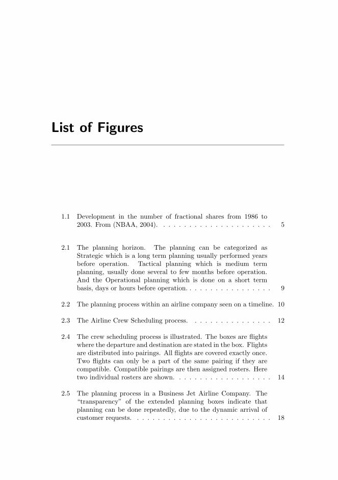
List of Figures
1.1 Development in the number of fractional shares from 1986 to2003. From (NBAA, 2004). . . . . . . . . . . . . . . . . . . . . . 5
2.1 The planning horizon. The planning can be categorized asStrategic which is a long term planning usually performed yearsbefore operation. Tactical planning which is medium termplanning, usually done several to few months before operation.And the Operational planning which is done on a short termbasis, days or hours before operation. . . . . . . . . . . . . . . . . 9
2.2 The planning process within an airline company seen on a timeline. 10
2.3 The Airline Crew Scheduling process. . . . . . . . . . . . . . . . 12
2.4 The crew scheduling process is illustrated. The boxes are flightswhere the departure and destination are stated in the box. Flightsare distributed into pairings. All flights are covered exactly once.Two flights can only be a part of the same pairing if they arecompatible. Compatible pairings are then assigned rosters. Heretwo individual rosters are shown. . . . . . . . . . . . . . . . . . . 14
2.5 The planning process in a Business Jet Airline Company. The“transparency” of the extended planning boxes indicate thatplanning can be done repeatedly, due to the dynamic arrival ofcustomer requests. . . . . . . . . . . . . . . . . . . . . . . . . . . 18

LIST OF FIGURES 166
3.1 A paired duty, where Joe (CP = Captain) is paired with co-pilotBen (FO = First-Officer). A roster for Joe, consisting of hispaired duty with Ben on days 2-5 and EXC (exercise session) ondays 11-14. A schedule consisting of two rosters, the one for Joerepeated and for Ben his paired duty with Joe on days 2-5, SBY(standby duty) on days 6-8 and VAC (vacation) on 12-15. OFFdenotes Day Off. . . . . . . . . . . . . . . . . . . . . . . . . . . . 29
3.2 A single duty - a paired duty made up of one pair from figure 3.1,with both pilots in the pair, Joe (CP) and Ben (FO). This willbe defined as a single duty. . . . . . . . . . . . . . . . . . . . . . 29
3.3 A double duty - a paired duty made up of two pairs. The first pair(Joe and Ben) are as in figure 3.2, but as it is put together withanother pair (Joe and Eva) it becomes a double duty. Observehow the highest ranking pilots (Joe) is “covered” through hisentire duty by lower ranking pilots (Ben and Eva). . . . . . . . . 30
3.4 How to count the number of paired tour days per day: Count thenumber of pairs of pilots able to operate an aircraft, e.g. the halfdays assigned for traveling (TR) do not count as paired tour days.For example day 2 has 1
2 paired tour days due to the traveling.Day 5 has 1 paired tour day, each pair contributes with a 1
2 dueto their traveling. . . . . . . . . . . . . . . . . . . . . . . . . . . . 31
4.1 Different options for the planning horizon for January. Thehighest of the blue lines indicate the shortest possible horizon;this is the month of January and no further days. The followinglines below show other possible horizons, where the red indicatesthe planning horizon we have chosen to use. Note that the initialtime period of each month cannot be planned given that it hasalready been planned by the planning of the previous month. . . 38
4.2 The two ways of considering quarter-wise planning, either asregular calendar quarters or as running quarters. Runningquarters requires equal information regardless of the currentplanning month. The information needed when applying calenderquarters vary with the time location of the different months. . . . 39

LIST OF FIGURES 167
4.3 Constructed example of the consequences of different distri-butions of pre-assignments when using the objective functionmaximizing Paired Tour Days (PTD). (a) shows clustered pre-assignments influencing the profile of the solution graph with highand low peaks. (b) shows how evenly distributed pre-assignmentsdo not influence the profile as much. . . . . . . . . . . . . . . . . 43
4.4 Constructed example of possible consequences using the objectivefunction minimizing Sum of Negative Deviation (SoND). Bothsolution have the exact same objective value, (a) has all negativedeviation gathered within a couple of days and (b) has a verysmall negative deviation distributed evenly over all days. . . . . . 44
4.5 Constructed example of possible consequences using the objectivefunction minimizing Largest Negative Deviation (LND). (a)shows how a single day with bounded high negative deviationcan bound the entire planning; (b) shows a better behavior whereseveral different days with largest negative deviation exist. . . . . 46
4.6 The corresponding Availability Matrix for a work plan. Anexample, a “6” means that a duty can be started on that dayand last six days. The codes are: OFF (day off) does not requirebuffer; VAC (vacation) does not require buffer; EXC (exercise)does require buffer of woff . Possible values in the AvailabilityMatrix are {0, . . . , wmax} = {0, 1, 2, 3, 4, 5, 6}. . . . . . . . . . . . 49
4.7 The corresponding Availability Matrix for a work plan. Anexample, a “6” means that a duty can be started on that dayand last six days. The codes are: OFF (day off) does not requirebuffer; VAC (vacation) does not require buffer; EXC (exercise)does require buffer of woff . Possible values in the AvailabilityMatrix are {0, wmin, . . . , wmax} = {0, 3, 4, 5, 6}. . . . . . . . . . . 50
6.1 An eight day schedule for three pilots is illustrated in the top ofthe illustration. The same schedule is shown below. This is thecorresponding representation of the schedule in the BIP model.The variables are all 0 except for the variables representing thetime and pilots to whom the duty is assigned. . . . . . . . . . . . 67
6.2 Constraining the maximal consecutive working days; wmax = 6. . 68
6.3 Ensuring the minimal consecutive working days; wmin = 3. . . . 68

LIST OF FIGURES 168
6.4 Ensuring the minimal consecutive days-off; woff = 5. . . . . . . . 70
6.5 Number of variables for fixed values of j = 30 and t = 2. Equaldistribution of pilot ranks, Captains and First-officers. . . . . . . 73
6.6 Number of constraints for fixed values of j = 30 and t = 2. Equaldistribution of pilot ranks, Captains and First-officers. . . . . . . 75
7.1 Network, where each arc has a capacity of 1. Node s is the sourcenode and node t is the sink node. . . . . . . . . . . . . . . . . . . 77
7.2 Here the same basic network as in figure 7.1 is shown, except forthe number of commodities. Here we now have two commodities.The arcs shared by the commodities now have a capacity of 2, soboth commodities can maintain a flow of maximum 1 and henceflow unrestricted. . . . . . . . . . . . . . . . . . . . . . . . . . . . 78
7.3 The nodes represent actions in each time period. The duty nodesare constructed for each possible pair of pilots, telling which pilotswork together. . . . . . . . . . . . . . . . . . . . . . . . . . . . . 80
7.4 The connections in the beginning and end of a period. . . . . . . 82
7.5 Connections so pilots can perform the same action over severaltime periods. . . . . . . . . . . . . . . . . . . . . . . . . . . . . . 83
7.6 The full network over four days, without pre-assignments. Herethe pilots can change action. . . . . . . . . . . . . . . . . . . . . 83
7.7 The transformation of a schedule containing the rosters of twopilots into a flow in the network (shown by the bold arcs). Notehow flow into day 2 goes from OFF to TR and half a day laterto the pair. Hereafter the flow continues from pair to pair nodeand finally on day 5 goes down to OFF through TR. . . . . . . . 84
7.8 Constraining minimum working days in the network model;wmin = 3. The bold arcs show the flow in the network, red arcsthe path that becomes infeasible and the arc with ”no entry” signmark the arc that constraint (7.5h) prohibits. A shows an illegalpath and B shows a legal. . . . . . . . . . . . . . . . . . . . . . . 88

LIST OF FIGURES 169
7.9 Constraining maximum working days in the network model;wmax = 6. The bold arcs show the flow in the network, redarcs show the path that becomes infeasible and the arc with the”no entry” sign mark the flow that constraint (7.5g) prohibits. . 89
7.10 Constraining minimum consecutive days-off after a duty periodin the network model; woff = 5. The bold arcs show the flowin the network, red arcs show the path leading to the flow thatconstraint (7.5i) prohibits, illustrated with the ”no entry” signs. . 90
7.11 The pre-assignment nodes are constructed and connections areestablished. The arcs showed are the newly constructed ones,while the rest of the connections in the network are left out. . . . 91
7.12 Depiction of an exercise session pre-assigned for two pilotstransformed into the structure of the network. Observe how it isonly possible to flow among pre-assignment arcs on days 4-6. . . 93
7.13 Number of variables for fixed values of j = 30 and t = 2. Assumedequal distribution of pilot ranks, Captains (both normal and low-timers) and First-Officer (both normal and low-timers). . . . . . 97
7.14 Number of constraints for fixed values of j = 30 and t = 2.Assumed equal distribution of pilot ranks, captain, normal andlow-timer and first-officer, normal and low-timer. . . . . . . . . . 98
8.1 Illustration of a function with one global optimum and severallocal optima. In this case it is a maximization function so thehigher value, the better. . . . . . . . . . . . . . . . . . . . . . . . 101
8.2 Results of the parameter tuning for Simulated Annealing withobjective function Paired Tour Days for realistic datasets plottedin average percentage gap and standard deviation for eachparameter setting. Based on table D.2. There is not enough spacefor labeling each “sub”-probability, but within each temperatureTstart the sequence of the probabilities is the same as in table 8.2. 112
8.3 Results of the parameter tuning for Simulated Annealing withobjective function Paired Tour Days for generated datasetsplotted in average percentage gap and standard deviation for eachparameter setting. Based on table D.3. There is not enough spacefor labeling each “sub”-probability, but within each temperatureTstart the sequence of the probabilities is the same as in table 8.2. 113

LIST OF FIGURES 170
8.4 Results of the parameter tuning for Simulated Annealing with ob-jective function Largest Negative Deviation for generated datasetsplotted in average percentage gap and standard deviation for eachparameter setting. Based on table D.7. There is not enough spacefor labeling each “sub”-probability, but within each temperatureTstart the sequence of the probabilities is the same as in table 8.2. 115
8.5 Average percentage gap and average for Simulated Annealingwith the three objective functions. The percentage gap iscalculated against the average solution value at the 30 secondruns, e.g. a negative number means that the algorithm hasfound an improved solution in comparison with the solution at30 seconds. Observe that the graphs have double y-axis, one foraverage percentage gap and one for averages of averages (axisfollow colors of graphs). . . . . . . . . . . . . . . . . . . . . . . . 118
9.1 The interaction between the Master and Sub Problem is illus-trated. Dual values are produced when solving the restrictedMaster Problem. These are used in the Sub Problem to findpromising columns to introduce in the Master Problem. Thecolumns are transmitted back to the Master Problem, which isthen resolved. This continues until no dual values values provideinformation to generate new columns. . . . . . . . . . . . . . . . 123
9.2 Two examples of conflicting columns. In case A two dutiesoverlap in time and share a pilot; these exclude each other. In caseB the two duties also share a pilot, but do not overlap. Howeverthe duties exclude each other as there are not woff consecutivedays off between the two duties. In this case columns are alsoconflicting. . . . . . . . . . . . . . . . . . . . . . . . . . . . . . . 127
9.3 An example of how the Exclusion Matrix is constructed. Thereare four different duties. The columns excluded can be identifiedby looking at the Exclusion Matrix. . . . . . . . . . . . . . . . . 128
9.4 The calculation of buffer is performed on pilot level so othercolumns are not wrongly excluded because of wrong buffercalculations. Case A show the per pilot level; case B per longestduty. We use the per pilot level. . . . . . . . . . . . . . . . . . . 128
9.5 The desired request area is found as the area of length wmin withthe largest sum of deviation from demand s−j,t in the time units. . 133

LIST OF FIGURES 171
9.6 For a given request area the column candidates to introduce inthe RMP are illustrated. All duties cover the area fully. . . . . . 134
9.7 Schematic representation of the Column Matheuristic (CMH). . . 135
9.8 The variation of the column pool size when introducing anddeleting columns in each iteration. . . . . . . . . . . . . . . . . . 139
9.9 The effect of the penalty list. The lack according to demandis given over a six iteration period. When a area is selected(illustrated by the grey box) a penalty of one is added to reducethe lack. If all areas are equal the earliest located area is chosen.Observe how the area {1, 2, 3} is not chosen in iteration E and F. 140
9.10 Results of the parameter tuning for Column Matheuristic withobjective function Paired Tour Days plotted in average percent-age gap and standard deviation for each parameter setting. Basedon table E.2 in appendix. . . . . . . . . . . . . . . . . . . . . . . 144
9.11 Results of the parameter tuning for Column Matheuristic withobjective function Sum Of Negative Deviation plotted in aver-age percentage gap and standard deviation for each parametersetting. Based on table E.2 in appendix. . . . . . . . . . . . . . . 144
9.12 Results of the parameter tuning for Column Matheuristic withobjective function Largest Negative Deviation plotted in averagepercentage gap and standard deviation for each parameter set-ting. Based on table E.2 in appendix. . . . . . . . . . . . . . . . 145
10.1 Profile of solution for the dataset Test2007-03 with normaldemand. This solution has a objective value for PTD=489. . . . 154
A.1 Demonstration of calculating the maximum available pairs, PAIRSMAX .179
D.1 Results of the parameter tuning for Simulated Annealing with ob-jective function Sum Of Negative Deviation for realistic datasetsplotted in average percentage gap and standard deviation for eachparameter setting. Based on table D.4. There is not enough spacefor labeling each “sub”-probability, but within each temperatureTstart the sequence of the probabilities is the same as in table 8.2. 199

LIST OF FIGURES 172
D.2 Results of the parameter tuning for Simulated Annealing with ob-jective function Sum Of Negative Deviation for generated datasetsplotted in average percentage gap and standard deviation for eachparameter setting. Based on table D.5. There is not enough spacefor labeling each “sub”-probability, but within each temperatureTstart the sequence of the probabilities is the same as in table 8.2. 200
D.3 Results of the parameter tuning for Simulated Annealing with ob-jective function Largest Negative Deviation for realistic datasetsplotted in average percentage gap and standard deviation for eachparameter setting. Based on table D.6. There is not enough spacefor labeling each “sub”-probability, but within each temperatureTstart the sequence of the probabilities is the same as in table 8.2. 201

List of Tables
1.1 Relative differences on various topics between Business JetAirlines and regular Commercial Airlines. . . . . . . . . . . . . . 6
1.2 List of some major Business Jet Airline Companies. . . . . . . . 7
2.1 Descriptions and literature references of application areas forpersonnel scheduling problems. . . . . . . . . . . . . . . . . . . . 24
3.1 Overview of which rules apply for the different events. [R1]:Min consecutive days-off, [R2]: Min duty length, [R3]: Max dutylength, [R4]: Min length of event type, [R5]: Max work month,[R6]: Max work quarter, [R7]: Travel in duty, [R8]: Standby days. 34
4.1 Overview of objective functions. Respectively columns variablesand constraints state how many extra of the kind are introducedwith the objective function. U denotes a planning unit, in thisproblem a time period, i.e. variables 2 ·U denotes that 2 variablesare introduced per time unit. Parenthesis indicate the equationin which variables and constraints are stated. . . . . . . . . . . . 47
LIST OF TABLES 174
5.1 Overview of datasets used for experimental results. Note that forall sets there is a normal version with regards to demand and aversion with peak(s), i.e. there are two dataset for every row inthe table. Hence there are 28 datasets in total, 14 with normaldemand and 14 with peak demand. . . . . . . . . . . . . . . . . . 58
5.2 Listing of the codes used. Specifications for each code are given.(a) TR requires buffer in the sense that it is located directly upto a paired duty which requires buffer. (b) The only code that isregistered as demand satisfying is the paired duty (#). . . . . . . 59
5.3 Overview of the specifications for all datasets. . . . . . . . . . . . 60
5.4 Overview of the specifications for all datasets. . . . . . . . . . . . 61
6.1 Listing of the four possible cases in (6.2). . . . . . . . . . . . . . 69
6.2 Number of constraints in the basic model divided into thedifferent constraint types. . . . . . . . . . . . . . . . . . . . . . . 74
6.3 Solution time for the two instances are given in the third column.The number of pilots is given for each of the instances. Numberof days is 30 and number of time periods is 2. . . . . . . . . . . . 75
7.1 Number of variables/possible flow in the model divided intodifferent arcs in the network. A ” ∗ ” in the stated variablesindicate that all possible values are included. . . . . . . . . . . . 95
7.2 Number of constraints in the model divided into the differentconstraint types. . . . . . . . . . . . . . . . . . . . . . . . . . . . 98
7.3 Solution time for three instances are given in the third column.The number of pilots are given. Equal distribution between low-timer captains and normal first-officers, no pilots with differentrank in the problems. Number of days is 30 and number of timeperiods is 2. . . . . . . . . . . . . . . . . . . . . . . . . . . . . . . 99
8.1 Fixed settings for parameter tuning of the Simulated Annealingalgorithm. . . . . . . . . . . . . . . . . . . . . . . . . . . . . . . . 109
LIST OF TABLES 175
8.2 Parameters and tested values for parameter tuning of the Simu-lated Annealing algorithm. . . . . . . . . . . . . . . . . . . . . . . 111
8.3 Found settings from parameter tuning of Simulated Annealing. . 116
8.4 Overview of average found solutions z, standard deviations σ andbest found solutions z∗ with SA for the three objective functionsPaired Tour Days (PTD). Sum of Negative Deviation (SoND) andLargest Negative Deviation (LND) over all test datasets. Averagestandard deviation σ is also calculated. . . . . . . . . . . . . . . . 120
9.1 The size of the model in the Master Problem. There are onebinary variable for each column included. There are |C| + |P |constraints in the problem, i.e. the number of columns includeplus the number of pilots in the problem instance. . . . . . . . . 131
9.2 Fixed settings for parameter tuning of the Column Matheuristic. 142
9.3 Parameters and tested values for parameter tuning of the Simu-lated Annealing algorithm. . . . . . . . . . . . . . . . . . . . . . . 143
9.4 Found settings from parameter tuning of Column Matheuristic. . 146
9.5 Overview of average found solutions z, standard deviations σand best found solutions z∗ with CMH for the three objectivefunctions Paired Tour Days (PTD). Sum of Negative Deviation(SoND) and Largest Negative Deviation (LND) over all testdatasets. Average standard deviation σ is also calculated. . . . . 147
10.1 Overview of solution approaches in this thesis. ∗: the maximumproblem sizes of 30 days and 2 time periods that the solutionapproaches can solve. . . . . . . . . . . . . . . . . . . . . . . . . . 149
10.2 Comparison of SA and CMH for the objective function PTD.For each solution approach is listed the average found solutionsz, standard deviations σ and best found solution z∗. Thecomparison columns are the percentage improvement for theCMH over the SA, i.e. positive numbers denotes improvement(CMH better than SA) and the negative the opposite. . . . . . . 150
LIST OF TABLES 176
10.3 Summary of comparison of SA and CMH for all objectivefunctions. For each solution approach is listed the improvement inaverage found solutions z, standard deviations σ and best foundsolutions z∗. The percentages are the percentage improvement forthe CMH over the SA, i.e. positive numbers denotes improvement(CMH better than SA). Finally a weighted average is shown(realistic datasets with weight 8 and generated with 6); a is wherethe weights 8-6 are not possible, where weights are correspondingto the number of available results for each type. . . . . . . . . . . 151
10.4 Comparison of average and best found solution values of testingdatasets to bounds. The percentage gaps to the bound are shownfor both average and best found solutions. . . . . . . . . . . . . . 152
A.1 Overview of the bounds on the tuning datasets . . . . . . . . . . 179
D.1 Summary of tuning for the best parameter settings for SimulatedAnnealing. Overview of average found solutions z, standarddeviations σ and best found solutions z∗ with SA for the threeobjective functions Paired Tour Days (PTD), Sum of NegativeDeviation (SoND) and Largest Negative Deviation (LND) overall test datasets. Average standard deviation σ is also calculated. 198
D.2 Parameter tuning results for SA with the objective functionPaired Tour Days and realistic datasets (Sample size 5; 30 secondsper sample). . . . . . . . . . . . . . . . . . . . . . . . . . . . . . . 202
D.3 Parameter tuning results for SA with the objective functionPaired Tour Days and generated datasets (Sample size 5; 30seconds per sample). . . . . . . . . . . . . . . . . . . . . . . . . . 203
D.4 Parameter tuning results for SA with the objective function Sumof Negative Deviation and realistic datasets (Sample size 5; 30seconds per sample). . . . . . . . . . . . . . . . . . . . . . . . . . 204
D.5 Parameter tuning results for SA with the objective function Sumof Negative Deviation and generated datasets (Sample size 5; 30seconds per sample). . . . . . . . . . . . . . . . . . . . . . . . . . 205
D.6 Parameter tuning results for SA with the objective functionLargest Negative Deviation and realistic datasets (Sample size5; 30 seconds per sample). . . . . . . . . . . . . . . . . . . . . . . 206

LIST OF TABLES 177
D.7 Parameter tuning results for SA with the objective functionLargest Negative Deviation and generated datasets (Sample size5; 30 seconds per sample). . . . . . . . . . . . . . . . . . . . . . . 207
E.1 Summary of tuning for the best parameter settings for ColumnMatheuristic. Overview of average found solutions z, standarddeviations σ and best found solutions z∗ with SA for the threeobjective functions Paired Tour Days (PTD), Sum of NegativeDeviation (SoND) and Largest Negative Deviation (LND) overall tuning datasets. Average standard deviation σ is also calculated.209
E.2 Results of tuning for the parameter setting for Column Matheuris-tic. Overview of average percentage gap (or average of averages)z and standard deviations σ for the three objective functionsPaired Tour Days (PTD), Sum of Negative Deviation (SoND)and Largest Negative Deviation (LND) over all tuning datasets.These results are illustrated in figure 9.10, 9.11 and 9.12 on pages144 to 144. . . . . . . . . . . . . . . . . . . . . . . . . . . . . . . 209
F.1 Comparison of SA and CMH for the objective function SoND.For each solution approach is listed the average found solutionsz, standard deviations σ and best found solutions z∗. Thecomparison columns are the percentage improvement for theCMH over the SA, i.e. positive numbers denotes improvement(CMH better than SA) and the negative the opposite. . . . . . . 211
F.2 Comparison of SA and CMH for the objective function LND.For each solution approach is listed the average found solutionsz, standard deviations σ and best found solutions z∗. Thecomparison columns are the percentage improvement for theCMH over the SA, i.e. positive numbers denotes improvement(CMH better than SA) and the negative the opposite. . . . . . . 211

Appendix A
Bounds and Data
A.1 Calculating Maximum Available Pairs
In table A.1 a demonstration of how to calculate the maximum available pairsin a time unit is illustrated. The formula is given in section 4.5.
A.2 Data Specifications
Bounds on tuning datsets. The formulas for calculating the bounds are given insection 4.5. Bounds on the testing datasets are shown in section 5.4.

A.2 Data Specifications 179
Figure A.1: Demonstration of calculating the maximum available pairs, PAIRSMAX .
Dataset Demand Rank Days PTD LND
Tune2007-01 Normal {54, 16, 32, 21} 31 1052 2Tune2007-01 Peak {54, 16, 32, 21} 31 1052 2Tune2007-02 Normal {54, 16, 32, 22} 28 1080 0Tune2007-02 Peak {54, 16, 32, 22} 28 1080 0Tune2007-12 Normal {82, 18, 45, 19} 31 1269 3Tune2007-12 Peak {82, 18, 45, 19} 31 1269 3Tune2008-01 Normal {82, 18, 45, 27} 31 1428 6Tune2008-01 Peak {82, 18, 45, 27} 31 1428 6TuneEmpty Normal {80, 20, 50, 30} 31 2790 0TuneEmpty Peak {80, 20, 50, 30} 31 2790 0TuneSparse1 Normal {60, 20, 30, 0} 28 1335 0TuneSparse1 Peak {60, 20, 30, 30} 28 1616 0TuneSparse2 Normal {60, 20, 30, 30} 28 1616 0TuneSparse2 Peak {60, 20, 30, 30} 28 1616 0
Table A.1: Overview of the bounds on the tuning datasets

Appendix B
Implementation in MoselXpress-MP
Listed here are the implementations of the BIP model described in chapter 6 aswell as the Network Flow Model described in chapter 7.
B.1 Binary Integer Model
!-------------------------- DTU Transport -----------------------
!----------------------------------------------------------------
!-------- Thesis title: Rostering for Business Jet Airline ------
!----------------------------------------------------------------
!------------Alex Chizeck Andersen and Charlotte Funch-----------
!----------------------------------------------------------------
!-----------------------------April 2008-------------------------
!----------------------------------------------------------------
!MOSEL model of the BIP.
!An implementation of the basic model.
!----------------------------------------------------------------
model TestModel2
uses "mmxprs";

B.1 Binary Integer Model 181
declarations
status:array({XPRS_OPT,XPRS_UNF,XPRS_INF,XPRS_UNB}) of string
end-declarations
status:=["Optimum found","Unfinished","Infeasible","Unbounded"]
COST_D_M := 1
COST_D_P := -1
COST_CP := 0
COST_FO := 0
TIME := {"am", "pm"}
DAYS := 1..30
PILOTS_CP := 101..102
PILOTS_FO := 201..202
PILOTS := PILOTS_CP + PILOTS_FO
ACT_TR := 666
PILOTS_DUTYACT := {ACT_TR} !666 svarer til træning
ALLDUTYACT := PILOTS + PILOTS_DUTYACT
declarations
DEMAND : array(DAYS,TIME) of integer
end-declarations
DEMAND := [1,1,1,1,1,1,1,1,1,1,1,1,1,1,1,1,1,1,1,1,1,1,1,1,1,1,1,
1,1,1,1,1,1,1,1,1,1,1,1,1,1,1,1,1,1,1,1,1,1,1,1,1,1,1,1,1]
declarations
x : array(PILOTS,DAYS,TIME,ALLDUTYACT) of mpvar
d_p : array(DAYS,TIME) of mpvar !plus
d_m : array(DAYS,TIME) of mpvar !minus
end-declarations
forall(p1 in PILOTS, j in DAYS, t in TIME, a in ALLDUTYACT)
x(p1,j,t,a) is_binary
! Constraints ---------------------------------------------------
! Mød demand - finder med d_p og d_m ud af hvor langt fra +/-
forall(j in DAYS, t in TIME)
MeetDemand(j,t) := sum(p1 in PILOTS, p2 in PILOTS) x(p1,j,t,p2)
- d_p(j,t) + d_m(j,t) = 2*DEMAND(j,t)
! Max arbejdsdage i maned
forall(p1 in PILOTS)
MaxWorkInMonth(p1) := sum(j in DAYS, t in TIME, a in ALLDUTYACT)
x(p1,j,t,a) <= 50*2

B.1 Binary Integer Model 182
! Max arbejdsdage i work period
forall(p1 in PILOTS, j in DAYS | DAYS(j) > 6)
MaxWorkConsecutive(p1,j) :=
sum(l in j-6..j, t in TIME, a in ALLDUTYACT) x(p1,l,t,a) <= 6*2
! Min arbejdsdage i work period
(virker først nar 5-dages ferie virker)
forall(p1 in PILOTS, j IN DAYS | DAYS(j) > 2 AND DAYS(j) <
getsize(DAYS)-1) MinWorkConsecutive(p1,j) :=
sum(l in j-2..j+2, t in TIME, a in ALLDUTYACT)
x(p1,l,t,a) >= sum(t in TIME, a in ALLDUTYACT) 3*x(p1,j,t,a)
! Min dage fri
forall(p1 in PILOTS, j IN DAYS | DAYS(j) > 1 AND DAYS(j) <=
getsize(DAYS)-4) MinDaysOff(p1,j) := sum(l in j..j+4, t in TIME)
(1 - sum(a in ALLDUTYACT) x(p1,l,t,a)) >=
sum(t in TIME, a in ALLDUTYACT) 5*x(p1,j-1,t,a)
- sum(t in TIME, a in ALLDUTYACT) 6*x(p1,j,t,a)
! Quick workaround. 1+1 nar en dag er duty
forall(p1 in PILOTS, j IN DAYS) do
DoubleOneA(p1,j) := sum(t in TIME, a in ALLDUTYACT) x(p1,j,t,a) >=
sum(a in ALLDUTYACT) 2*x(p1,j,"am",a)
DoubleOneB(p1,j) := sum(t in TIME, a in ALLDUTYACT) x(p1,j,t,a) >=
sum(a in ALLDUTYACT) 2*x(p1,j,"pm",a)
end-do
! Begin og End-vagter:
forall(p1 in PILOTS, j IN DAYS | DAYS(j) >= 1)
DutyBegin(p1,j) := x(p1,j,"am",ACT_TR) >= sum(a in ALLDUTYACT)
(x(p1,j,"am",a) - x(p1,j-1,"pm",a))
forall(p1 in PILOTS, j IN DAYS | DAYS(j) <= getsize(DAYS))
DutyEnd(p1,j) := x(p1,j,"pm",ACT_TR) >= sum(a in ALLDUTYACT)
(x(p1,j,"pm",a) - x(p1,j+1,"am",a))
! Man ma ikke arbejde sammen med sig selv:
forall(p in PILOTS, j in DAYS, t in TIME)
NoWorkingTogetherWithSelf(p,j,t) := x(p,j,t,p) = 0
! Exactly two pilots must work together:
forall(p1 in PILOTS, j IN DAYS, t in TIME)
TwoPilotsMustWorkTogether(p1,j,t) := sum(a in ALLDUTYACT)
x(p1,j,t,a) <= 1
! Two pilots must agree on working together:
forall(p1 in PILOTS, j in DAYS, t in TIME, p2 in PILOTS)
TwoPilotsMustAgree(p1,j,t,p2) := x(p1,j,t,p2) = x(p2,j,t,p1)

B.1 Binary Integer Model 183
! Two FO can not work together:
forall(p_fo1 in PILOTS_FO, j in DAYS, t in TIME)
NoTwoFOsWorkTogether(p_fo1,j,t) := sum(p_fo2 in PILOTS_FO)
x(p_fo1,j,t,p_fo2) = 0
forall(p_cp1 in PILOTS_CP, j in DAYS, t in TIME)
NoTwoCPsWorkTogether(p_cp1,j,t) := sum(p_cp2 in PILOTS_CP)
x(p_cp1,j,t,p_cp2) = 0
! If a pilot switches pilot pairing to another, must travel two periods
forall(p1 in PILOTS_FO, j in DAYS | DAYS(j) <=
getsize(DAYS)-1, p2 in PILOTS_CP)
DoubleTravelBetweenSwitch(p1,j,p2) :=
x(p1,j,"pm",ACT_TR) + x(p1,j+1,"am",ACT_TR) + x(p1,j,"am",p2) +
3 * sum(pstar in PILOTS_CP | pstar <> p2) x(p1,j,"am",pstar) +
3 * x(p1,j,"am",ACT_TR) +
3 * (1 - sum(pstar in PILOTS) x(p1,j,"am",pstar)) >=
3 * sum(pstar in PILOTS_CP | pstar <> p2) x(p1,j+1,"pm",pstar)
! Limit number of TR within periods - different for FO and CP
forall(p in PILOTS_CP, j in DAYS | DAYS(j) <= getsize(DAYS)-5)
LimitOnCPTR(p,j) := sum(l in j..j+5, t in TIME) x(p,l,t,ACT_TR) <= 2
forall(p in PILOTS_FO, j in DAYS | DAYS(j) <= getsize(DAYS)-5)
LimitOnFOTR(p,j) := sum(l in j..j+5, t in TIME) x(p,l,t,ACT_TR) <= 4
! Sørger for at der ikke ma være flere TR’er end
!der er arbejde omkring.
! w TR TR w er lovlig.
forall(p in PILOTS, j in DAYS | DAYS(j) <= getsize(DAYS)-1)
NoTwoTravelIfNotInWorkPeriod(p,j) :=
x(p,j,"pm",ACT_TR) + x(p,j+1,"am",ACT_TR) <=
sum(p2 in PILOTS) x(p,j,"am",p2) +
sum(p2 in PILOTS) x(p,j+1,"pm",p2)
! Cannot work with two different pilots on to consecutive periods
! (there must be a switch, which requires TR).
forall(p1 in PILOTS_FO, j in DAYS, p2 in PILOTS_CP | p2 <> p1)
NoQuickPairingChangeAMtoPMfo(p1,j,p2) :=
x(p1,j,"am",p2) + sum(pstar in PILOTS_CP | pstar <> p2)
x(p1,j,"pm",pstar) <= 1
forall(p1 in PILOTS_FO, j in DAYS | DAYS(j) <=
getsize(DAYS)-1, p2 in PILOTS_CP | p2 <> p1)
NoQuickPairingChangePMtoAMfo(p1,j,p2) :=
x(p1,j,"pm",p2) + sum(pstar in PILOTS_CP | pstar <> p2)
x(p1,j+1,"am",pstar) <= 1
forall(p1 in PILOTS_CP, j in DAYS, p2 in PILOTS_FO | p2 <> p1)

B.1 Binary Integer Model 184
NoQuickPairingChangeAMtoPMcp(p1,j,p2) :=
x(p1,j,"am",p2) + sum(pstar in PILOTS_FO | pstar <> p2)
x(p1,j,"pm",pstar) <= 1
forall(p1 in PILOTS_CP, j in DAYS | DAYS(j) <=
getsize(DAYS)-1, p2 in PILOTS_FO | p2 <> p1)
NoQuickPairingChangePMtoAMcp(p1,j,p2) :=
x(p1,j,"pm",p2) + sum(pstar in PILOTS_FO | pstar <> p2)
x(p1,j+1,"am",pstar) <= 1
! Objective -----------------------------------------------------
Obj := sum(j in DAYS, t in TIME) d_m(j,t) - 10 *
sum(p1 in PILOTS, j in DAYS, t in TIME) x(p1,j,t,ACT_TR)
! End -----------------------------------------------------------
minimize(Obj)
! Print to scren ------------------------------------------------
writeln("Status: ", status(getprobstat))
writeln("Opt. obj. value: ", getsol(Obj))
writeln
forall(p1 in PILOTS_CP) do
write(PILOTS_CP(p1), ": ")
forall(j in DAYS) do
forall(t in TIME)
if sum(a in ALLDUTYACT) getsol(x(p1,j,t,a))<>0 then
if getsol(x(p1,j,t,ACT_TR)) = 1 then
write("T")
else
write(sum(a in ALLDUTYACT) getsol(x(p1,j,t,a)))
end-if
else
write("·")end-if
write(" ")
end-do
writeln
end-do
writeln
forall(p1 in PILOTS_FO) do
write(PILOTS_FO(p1), ": ")
forall(j in DAYS) do

B.1 Binary Integer Model 185
forall(t in TIME)
if sum(a in ALLDUTYACT) getsol(x(p1,j,t,a))<>0 then
if getsol(x(p1,j,t,ACT_TR)) = 1 then
write("T")
else
write(sum(a in ALLDUTYACT) getsol(x(p1,j,t,a)))
end-if
else
write("·")end-if
write(" ")
end-do
writeln
end-do
writeln
write("CPs: ")
forall(j in DAYS) do
forall(t in TIME)
write(sum(p_cp in PILOTS_CP, p2 in PILOTS)
getsol(x(p_cp,j,t,p2)), "")
write(" ")
end-do
writeln
write("FOs: ")
forall(j in DAYS) do
forall(t in TIME)
write(sum(p_fo in PILOTS_FO, p2 in PILOTS)
getsol(x(p_fo,j,t,p2)), "")
write(" ")
end-do
writeln
writeln
write("ACT: ")
forall(j in DAYS) do
forall(t in TIME)
write(sum(p in PILOTS) getsol(x(p,j,t,ACT_TR)), "")
write(" ")
end-do
writeln
writeln
write("D*2: ")
forall(j in DAYS) do
forall(t in TIME)

B.2 Multi-Commodity Network Flow Model 186
write(DEMAND(j,t))
write(" ")
end-do
writeln
write("d_m: ")
forall(j in DAYS) do
forall(t in TIME)
if getsol(d_m(j,t))<>0 then
write(getsol(d_m(j,t)), "")
else
write("·")end-if
write(" ")
end-do
writeln
write("d_p: ")
forall(j in DAYS) do
forall(t in TIME)
if getsol(d_p(j,t))<>0 then
write(getsol(d_p(j,t)), "")
else
write("·")end-if
write(" ")
end-do
end-model
B.2 Multi-Commodity Network Flow Model
!-------------------------- DTU Transport -----------------------
!----------------------------------------------------------------
!-------- Thesis title: Rostering for Business Jet Airline ------
!----------------------------------------------------------------
!------------Alex Chizeck Andersen and Charlotte Funch-----------
!----------------------------------------------------------------
!-----------------------------April 2008-------------------------
!----------------------------------------------------------------
!MOSEL model of the multi-commodity network flow problem.
!An implementation of the basic model.
!----------------------------------------------------------------
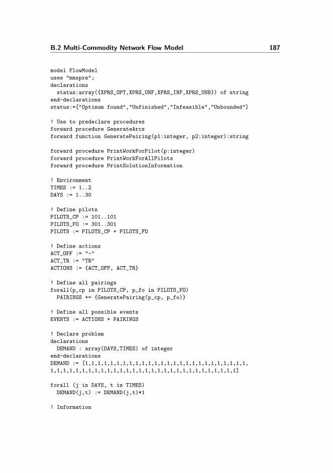
B.2 Multi-Commodity Network Flow Model 187
model FlowModel
uses "mmxprs";
declarations
status:array({XPRS_OPT,XPRS_UNF,XPRS_INF,XPRS_UNB}) of string
end-declarations
status:=["Optimum found","Unfinished","Infeasible","Unbounded"]
! Use to predeclare procedures
forward procedure GenerateArcs
forward function GeneratePairing(p1:integer, p2:integer):string
forward procedure PrintWorkForPilot(p:integer)
forward procedure PrintWorkForAllPilots
forward procedure PrintSolutionInformation
! Environment
TIMES := 1..2
DAYS := 1..30
! Define pilots
PILOTS_CP := 101..101
PILOTS_FO := 301..301
PILOTS := PILOTS_CP + PILOTS_FO
! Define actions
ACT_OFF := "-"
ACT_TR := "TR"
ACTIONS := {ACT_OFF, ACT_TR}
! Define all pairings
forall(p_cp in PILOTS_CP, p_fo in PILOTS_FO)
PAIRINGS += {GeneratePairing(p_cp, p_fo)}
! Define all possible events
EVENTS := ACTIONS + PAIRINGS
! Declare problem
declarations
DEMAND : array(DAYS,TIMES) of integer
end-declarations
DEMAND := [1,1,1,1,1,1,1,1,1,1,1,1,1,1,1,1,1,1,1,1,1,1,1,1,1,1,
1,1,1,1,1,1,1,1,1,1,1,1,1,1,1,1,1,1,1,1,1,1,1,1,1,1,1,1,1,1]
forall (j in DAYS, t in TIMES)
DEMAND(j,t) := DEMAND(j,t)*1
! Information

B.2 Multi-Commodity Network Flow Model 188
writeln("Number of possible pairings per time: ", getsize(PAIRINGS))
writeln("Number of possible pairings total: ", getsize(PAIRINGS)*
getsize(DAYS)*getsize(TIMES))
writeln("")
! Declare the arcs (variables)
declarations
x : dynamic array(PILOTS,EVENTS,EVENTS,DAYS,TIMES) of mpvar
! From event on j, t to event on j, t+1 (perhaps j+1,t)
x_o : dynamic array(PILOTS,EVENTS) of mpvar
x_d : dynamic array(EVENTS,PILOTS) of mpvar
s_p : array(DAYS,TIMES) of mpvar !plus
s_m : array(DAYS,TIMES) of mpvar !minus
end-declarations
! Generate the actual arcs (variables)
GenerateArcs
!----------------------------------------------------------------
! Only one action per period
writeln("Generating constraints OneActionPerPeriod: ")
forall (p in PILOTS, j in DAYS, t in TIMES | j > 1 AND j <
getsize(DAYS))
OneActionPerPeriod(p,j,t) :=
sum(e1 in EVENTS, e2 in EVENTS)
x(p,e1,e2,j,t) = 1
writeln(" > OK (normal cases)")
! Special case for origin and destination
forall (p in PILOTS) do
OneActionPerPeriodOrigin(p) :=
sum(e in EVENTS) x_o(p,e) = 1
OneActionPerPeriodDestination(p) :=
sum(e in EVENTS) x_d(e,p) = 1
end-do
writeln(" > OK (special cases)")
! Flow in must equal flow out
writeln("Generating constraints FlowInOutEqual:")
forall (p in PILOTS, j in DAYS, e in EVENTS) do
if (j > 1) then
FlowInOutEqualAM(p,j,e) :=
sum(eIN in EVENTS) x(p,eIN,e,j-1,2) =
sum(eOUT in EVENTS) x(p,e,eOUT,j,1)
end-if
if (j < getsize(DAYS)) then

B.2 Multi-Commodity Network Flow Model 189
FlowInOutEqualPM(p,j,e) :=
sum(eIN in EVENTS) x(p,eIN,e,j,1) =
sum(eOUT in EVENTS) x(p,e,eOUT,j,2)
end-if
end-do
writeln(" > OK (normal cases)")
! Special case for origin
forall (p in PILOTS, e in EVENTS)
FlowInOutOrigin(p,e) :=
x_o(p,e) =
sum(eOUT in EVENTS) x(p,e,eOUT,1,1)
! Special case for destination
forall (e in EVENTS, p in PILOTS)
FlowInOutDestination(e,p) :=
sum(eIN in EVENTS) x(p,eIN,e,getsize(DAYS),1) =
x_d(e,p)
writeln(" > OK (special cases)")
! Both or none pilot must enter a pairing
writeln("Generating constraints FlowIntoPairing (CP/FO): ")
forall (p_cp in PILOTS_CP, p_fo in PILOTS_FO) do
CurrentPairingCPFO := GeneratePairing(p_cp,p_fo)
forall (j in DAYS, t in TIMES | t < getsize(TIMES) OR j <
getsize(DAYS))
do
FlowIntoPairingCP := sum(eIN in EVENTS)
x(p_cp,eIN,CurrentPairingCPFO,j,t)
FlowIntoPairingFO := sum(eIN in EVENTS)
x(p_fo,eIN,CurrentPairingCPFO,j,t)
BothOrNoneCP(p_cp,p_fo,j,t) :=
FlowIntoPairingCP + FlowIntoPairingFO >= 2*FlowIntoPairingCP
BothOrNoneFO(p_fo,p_cp,j,t) :=
FlowIntoPairingCP + FlowIntoPairingFO >= 2*FlowIntoPairingFO
end-do
end-do
writeln(" > OK")
!-----------------------------------------------------------------
! Max arbejdsdage i work period
writeln("Generating constraints MaxWorkConsecutive: ")
w_max := 6
! Normal case
forall(p in PILOTS, j in DAYS | DAYS(j) < getsize(DAYS) - w_max)
MaxWorkConsecutive(p,j) :=

B.2 Multi-Commodity Network Flow Model 190
sum(l in j..j+w_max) x(p,ACT_TR,ACT_OFF,l,2) >=
x(p,ACT_OFF,ACT_TR,j,2)
writeln(" > OK (normal cases)")
! Special case: beginning
forall(p in PILOTS)
MaxWorkConsecutiveOrigin(p) :=
sum(l in 1..w_max+1, t in TIMES) x(p,ACT_TR,ACT_OFF,l,t) >=
sum(e in EVENTS | e <> ACT_OFF) x_o(p,e)
! Special case: end
forall(p in PILOTS)
MaxWorkConsecutiveDestination(p) :=
sum(l in getsize(DAYS)-w_max-1..getsize(DAYS), t in TIMES)
x(p,ACT_TR,ACT_OFF,l,t) + x_d(ACT_TR,p) + x_d(ACT_OFF,p) >=
x(p,ACT_OFF,ACT_TR,getsize(DAYS)-w_max-1,2)
writeln(" > OK (special cases)")
! Min duty days in working period
!(virker først nar 5-dages ferie virker)
writeln("Generating constraints MinWorkConsecutive: ")
w_min := 3
forall(p in PILOTS, j in DAYS | DAYS(j) < getsize(DAYS) - w_min)
MinWorkConsecutive(p,j) :=
sum(l in j+1..j+w_min-1) x(p,ACT_TR,ACT_OFF,l,2) <=
(1 - x(p,ACT_OFF,ACT_TR,j,2))
writeln(" > OK (normal cases)")
! Special case: beginning
forall(p in PILOTS)
MinWorkConsecutiveOrigin(p) :=
sum(l in 1..w_min-1) x(p,ACT_TR,ACT_OFF,l,2) <=
(1 - x_o(p,ACT_TR))
writeln(" > OK (special cases)")
! Min days off between work
writeln("Generating constraints MinDaysOff: ")
w_off := 5
! Normal case
forall(p in PILOTS, j in DAYS)
MinDaysOff(p,j) :=
sum(l in j+1..j+w_off, t in TIMES | l < j+w_off OR
t < getsize(TIMES)) x(p,ACT_OFF,ACT_OFF,l,t) >=
(2*w_off-1)*x(p,ACT_TR,ACT_OFF,j,2)
writeln(" > OK")
!-----------------------------------------------------------------
! Meet demand
writeln("Generating constraints MeetDemand: ")

B.2 Multi-Commodity Network Flow Model 191
forall(j in DAYS, t in TIMES) do
MeetDemand(j,t) := sum (p in PILOTS, e in EVENTS, pair in PAIRINGS)
x(p,pair,e,j,t) - s_p(j,t) + s_m(j,t) = 2*DEMAND(j,t)
end-do
writeln(" > OK")
! Objective function
writeln("Generating objective function: ")
Obj := sum(j in DAYS, t in TIMES) s_m(j,t)
writeln(" > OK")
!-----------------------------------------------------------------
!x(302,ACT_OFF,ACT_TR,1,2) = 1
!x(101,ACT_OFF,ACT_TR,8,2) = 1
!-----------------------------------------------------------------
writeln
writeln("Starting solver: ")
minimize(Obj)
writeln(" > Done")
!-----------------------------------------------------------------
writeln
writeln("Print of solution: ")
writeln
PrintWorkForAllPilots
writeln
PrintSolutionInformation
writeln
!-----------------------------------------------------------------
! Used for generating a pairing number
function GeneratePairing(p1:integer, p2:integer):string
returned := strfmt(p1,0) + "-" + strfmt(p2,0)
end-function
!-----------------------------------------------------------------
! Generates the arrays of arcs (all = 1 are existing)
procedure GenerateArcs
writeln("Generating arcs (variables): ")
!----------------------

B.2 Multi-Commodity Network Flow Model 192
! Between all normal pairings
forall(p_cp in PILOTS_CP, p_fo in PILOTS_FO, j in DAYS | j <
getsize(DAYS)) do
CurrentPairingCPFO := GeneratePairing(p_cp, p_fo)
if (j > 1) then
create(x(p_cp, CurrentPairingCPFO, CurrentPairingCPFO, j, 1))
create(x(p_fo, CurrentPairingCPFO, CurrentPairingCPFO, j, 1))
end-if
create(x(p_cp, CurrentPairingCPFO, CurrentPairingCPFO, j, 2))
create(x(p_fo, CurrentPairingCPFO, CurrentPairingCPFO, j, 2))
end-do
!----------------------
! To the pairing from the TRs
forall(p_cp in PILOTS_CP, p_fo IN PILOTS_FO, j in DAYS | j <
getsize(DAYS)) do
CurrentPairingCPFO := GeneratePairing(p_cp, p_fo)
create(x(p_cp, ACT_TR, CurrentPairingCPFO, j, 1))
create(x(p_fo, ACT_TR, CurrentPairingCPFO, j, 1))
end-do
! To the TRs from the pairings
forall(p_cp in PILOTS_CP, p_fo IN PILOTS_FO, j in DAYS | j > 1) do
CurrentPairingCPFO := GeneratePairing(p_cp, p_fo)
create(x(p_cp, CurrentPairingCPFO, ACT_TR, j, 1))
create(x(p_fo, CurrentPairingCPFO, ACT_TR, j, 1))
end-do
!----------------------
! From days-off to TR (only to TR in AM, begin of new day)
! (has an exception on day last-1 pm,
!where only FO can go from OFF to TR.
forall(p in PILOTS, j in DAYS | j < getsize(DAYS)) do
if (j < getsize(DAYS) - 1) then
create(x(p, ACT_OFF, ACT_TR, j, 2))
end-if
end-do
! From TR to days-off (only to days-off in AM, begin of new day)
! (has an exception on day 1pm, where only FO
!can stop a TR with OFF.
forall(p in PILOTS, j in DAYS | j < getsize(DAYS)) do
create(x(p, ACT_TR, ACT_OFF, j, 2))
end-do
! From TR to TR (only for FOs, and only on a day, e.g. PM->AM)
forall(p_fo in PILOTS_FO, j in DAYS) do

B.2 Multi-Commodity Network Flow Model 193
create(x(p_fo, ACT_TR, ACT_TR, j, 2))
end-do
!----------------------
! Go from OFF to OFF (simple)
forall(p in PILOTS, j in DAYS) do
create(x(p, ACT_OFF, ACT_OFF, j, 1))
if (j < getsize(DAYS)) then
create(x(p, ACT_OFF, ACT_OFF, j, 2))
end-if
end-do
!----------------------
!----------------------
!----------------------
! All pilots can either TR or OFF
forall(p in PILOTS) do
create(x_o(p, ACT_TR))
create(x_o(p, ACT_OFF))
end-do
!----------------------
!----------------------
!----------------------
! All pilots can either TR or OFF
forall(p in PILOTS) do
create(x_d(ACT_TR, p))
create(x_d(ACT_OFF, p))
end-do
!----------------------
! Declare binary
forall (p in PILOTS, e1 in EVENTS, e2 in EVENTS, j in DAYS,
t in TIMES | exists(x(p,e1,e2,j,t)))
x(p,e1,e2,j,t) is_binary
forall (p in PILOTS, e in EVENTS | exists(x_o(p,e)))

B.2 Multi-Commodity Network Flow Model 194
x_o(p,e) is_binary
forall (e in EVENTS, p in PILOTS | exists(x_d(e,p)))
x_d(e,p) is_binary
!----------------------
writeln(" > OK")
end-procedure
!-----------------------------------------------------------------
!-----------------------------------------------------------------
procedure PrintWorkForAllPilots
write(",")
forall (j in DAYS, t in TIMES)
write("’", j, "/", t, ",")
writeln
forall (p_cp in PILOTS_CP)
PrintWorkForPilot(p_cp)
writeln
forall (p_fo in PILOTS_FO)
PrintWorkForPilot(p_fo)
end-procedure
procedure PrintWorkForPilot(p:integer)
write("’", p, ":,")
forall (j in DAYS, t in TIMES, e1 IN EVENTS, e2 IN EVENTS |
getsol(x(p,e1,e2,j,t)) > 0)
write(e1, ",")
forall (e in EVENTS | getsol(x_d(e,p)) > 0)
write(e, ",")
writeln
end-procedure
procedure PrintSolutionInformation
write("’j-:,")
forall(j in DAYS, t in TIMES)
write("-", getsol(s_m(j,t)), ",")
writeln
write("’j+:,")
forall(j in DAYS, t in TIMES)
write(getsol(s_p(j,t)), ",")
end-procedure
end-model

Appendix C
Implementation in C#
This appendix will serve as a brief description of the structure of the C#program. This covers both the implementation of the Simulated Annealingand the Column Matheuristic. The solution is split into five packages (thatreference each other when necessary). In total the solution has 7242 lines ofcode, including comments and blank lines.
Business Jet Airlines Rostering Problem: contains the main entry pointfor the application. Additionally it contains classes used for the “mass”-runs for parameter tuning and testing. (This package contains 614 linesof code).
Simulated Annealing: contains all classes used for the heuristic. Can berun on its own or can be call from the Column Matheuristic with specialparameters when used for warmstarts and area search. (This packagecontains 1918 lines of code).
Column Matheuristic: contains all classes used for the Matheuristic. Thecallable library Mosel Xpress-BCL must be present on the computer itused on, for solving the integer problems. (This package contains 1585lines of code).
Input and Output: classes and utilities used for reading in datasets, ana-lyzing, and writing solutions out. The solution format is standardized,

196
both the SA and the CMH send their solutions to the same solution classensuring a consistent design. (This package contains 2311 lines of code).
Toolbox: contains various utilities and structures used locally and globallythrough the application. Furthermore it contains all the “hard coded”settings in a designated class for easier further implementation. (Thispackage contains 814 lines of code).

Appendix D
Simulated Annealing - Tuningand Testing
D.1 Parameter Tuning
D.1.1 Summary
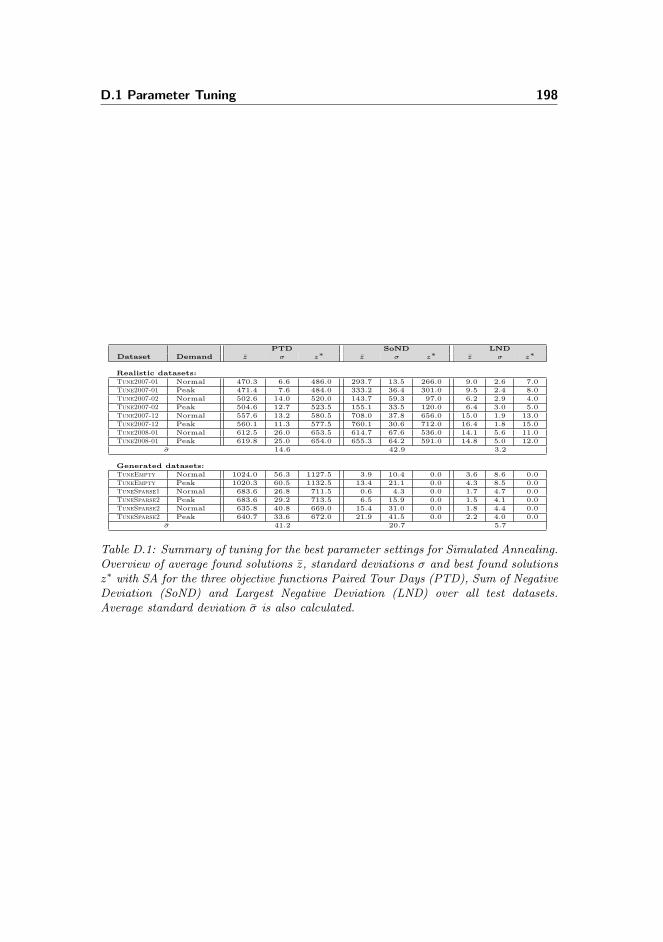
D.1 Parameter Tuning 198
PTD SoND LNDDataset Demand z σ z∗ z σ z∗ z σ z∗
Realistic datasets:
Tune2007-01 Normal 470.3 6.6 486.0 293.7 13.5 266.0 9.0 2.6 7.0Tune2007-01 Peak 471.4 7.6 484.0 333.2 36.4 301.0 9.5 2.4 8.0Tune2007-02 Normal 502.6 14.0 520.0 143.7 59.3 97.0 6.2 2.9 4.0Tune2007-02 Peak 504.6 12.7 523.5 155.1 33.5 120.0 6.4 3.0 5.0Tune2007-12 Normal 557.6 13.2 580.5 708.0 37.8 656.0 15.0 1.9 13.0Tune2007-12 Peak 560.1 11.3 577.5 760.1 30.6 712.0 16.4 1.8 15.0Tune2008-01 Normal 612.5 26.0 653.5 614.7 67.6 536.0 14.1 5.6 11.0Tune2008-01 Peak 619.8 25.0 654.0 655.3 64.2 591.0 14.8 5.0 12.0
σ 14.6 42.9 3.2
Generated datasets:
TuneEmpty Normal 1024.0 56.3 1127.5 3.9 10.4 0.0 3.6 8.6 0.0TuneEmpty Peak 1020.3 60.5 1132.5 13.4 21.1 0.0 4.3 8.5 0.0TuneSparse1 Normal 683.6 26.8 711.5 0.6 4.3 0.0 1.7 4.7 0.0TuneSparse2 Peak 683.6 29.2 713.5 6.5 15.9 0.0 1.5 4.1 0.0TuneSparse2 Normal 635.8 40.8 669.0 15.4 31.0 0.0 1.8 4.4 0.0TuneSparse2 Peak 640.7 33.6 672.0 21.9 41.5 0.0 2.2 4.0 0.0
σ 41.2 20.7 5.7
Table D.1: Summary of tuning for the best parameter settings for Simulated Annealing.Overview of average found solutions z, standard deviations σ and best found solutionsz∗ with SA for the three objective functions Paired Tour Days (PTD), Sum of NegativeDeviation (SoND) and Largest Negative Deviation (LND) over all test datasets.Average standard deviation σ is also calculated.

D.1 Parameter Tuning 199
D.1.2 Illustrations
Figure D.1: Results of the parameter tuning for Simulated Annealing with objectivefunction Sum Of Negative Deviation for realistic datasets plotted in average percentagegap and standard deviation for each parameter setting. Based on table D.4. There isnot enough space for labeling each “sub”-probability, but within each temperature Tstart
the sequence of the probabilities is the same as in table 8.2.

D.1 Parameter Tuning 200
Figure D.2: Results of the parameter tuning for Simulated Annealing with objectivefunction Sum Of Negative Deviation for generated datasets plotted in averagepercentage gap and standard deviation for each parameter setting. Based on table D.5.There is not enough space for labeling each “sub”-probability, but within eachtemperature Tstart the sequence of the probabilities is the same as in table 8.2.

D.1 Parameter Tuning 201
Figure D.3: Results of the parameter tuning for Simulated Annealing with objectivefunction Largest Negative Deviation for realistic datasets plotted in average percentagegap and standard deviation for each parameter setting. Based on table D.6. There isnot enough space for labeling each “sub”-probability, but within each temperature Tstart
the sequence of the probabilities is the same as in table 8.2.

D.1 Parameter Tuning 202
D.1.3 Tables
Tstart Probs. Avg.Gap Avg.StdDev Tstart Probs. Avg.Gap Avg.StdDev
1 0.3, 0.2, 0.5 6, 36% 8, 7 300 0.3, 0.2, 0.5 8, 65% 10, 921 0.3, 0.3, 0.4 6, 16% 8, 4 300 0.3, 0.3, 0.4 7, 07% 8, 681 0.4, 0.1, 0.5 6, 17% 8, 89 300 0.4, 0.1, 0.5 6, 4% 9, 361 0.4, 0.2, 0.4 6, 59% 7, 48 300 0.4, 0.2, 0.4 4, 76% 4, 731 0.4, 0.3, 0.3 6, 7% 7, 61 300 0.4, 0.3, 0.3 3, 72% 4, 211 0.4, 0.4, 0.2 6, 95% 8, 39 300 0.4, 0.4, 0.2 3, 03% 3, 971 0.5, 0.1, 0.4 6, 52% 8, 01 300 0.5, 0.1, 0.4 3, 36% 2, 841 0.5, 0.2, 0.3 6, 57% 9, 03 300 0.5, 0.2, 0.3 2, 33% 2, 771 0.5, 0.3, 0.2 7, 22% 8, 49 300 0.5, 0.3, 0.2 2, 22% 2, 541 0.5, 0.4, 0.1 6, 77% 8, 68 300 0.5, 0.4, 0.1 2, 66% 3, 741 0.5, 0.5, 0.0 7, 54% 8, 77 300 0.5, 0.5, 0.0 2, 47% 2, 271 0.6, 0.1, 0.3 7, 21% 10, 22 300 0.6, 0.1, 0.3 2, 27% 2, 631 0.6, 0.2, 0.2 6, 63% 11, 33 300 0.6, 0.2, 0.2 1, 95% 3, 181 0.6, 0.3, 0.1 6, 96% 11, 09 300 0.6, 0.3, 0.1 1, 99% 2, 411 0.6, 0.4, 0.0 7, 72% 10, 98 300 0.6, 0.4, 0.0 2, 4% 3, 151 0.7, 0.1, 0.2 7, 25% 11, 78 300 0.7, 0.1, 0.2 2, 22% 3, 061 0.7, 0.2, 0.1 7, 12% 11, 63 300 0.7, 0.2, 0.1 2, 16% 2, 881 0.7, 0.3, 0.0 8, 42% 16, 63 300 0.7, 0.3, 0.0 2, 33% 3, 191 0.8, 0.1, 0.1 7, 4% 12, 17 300 0.8, 0.1, 0.1 2, 12% 2, 761 0.8, 0.2, 0.0 7, 8% 11, 29 300 0.8, 0.2, 0.0 2, 57% 2, 881 0.9, 0.1, 0.0 7, 73% 10, 84 300 0.9, 0.1, 0.0 2, 53% 3, 53
100 0.3, 0.2, 0.5 5, 42% 8, 2 400 0.3, 0.2, 0.5 9, 3% 14, 49100 0.3, 0.3, 0.4 4, 88% 7, 69 400 0.3, 0.3, 0.4 8, 25% 8, 31100 0.4, 0.1, 0.5 4, 09% 4, 26 400 0.4, 0.1, 0.5 6, 52% 9, 03100 0.4, 0.2, 0.4 3, 69% 4, 59 400 0.4, 0.2, 0.4 5, 12% 7, 3100 0.4, 0.3, 0.3 3, 13% 3, 72 400 0.4, 0.3, 0.3 3, 66% 3, 72100 0.4, 0.4, 0.2 2, 87% 3, 69 400 0.4, 0.4, 0.2 3, 12% 3, 1100 0.5, 0.1, 0.4 2, 85% 3, 45 400 0.5, 0.1, 0.4 3, 23% 3, 59100 0.5, 0.2, 0.3 2, 2% 2, 73 400 0.5, 0.2, 0.3 2, 39% 3, 1100 0.5, 0.3, 0.2 2, 1% 3, 55 400 0.5, 0.3, 0.2 2, 09% 3, 12100 0.5, 0.4, 0.1 2, 55% 2, 45 400 0.5, 0.4, 0.1 2, 58% 3, 47100 0.5, 0.5, 0.0 2, 44% 2, 95 400 0.5, 0.5, 0.0 2, 42% 3, 56100 0.6, 0.1, 0.3 2, 02% 2, 61 400 0.6, 0.1, 0.3 2, 09% 3, 36100 0.6, 0.2, 0.2 2, 09% 3, 2 400 0.6, 0.2, 0.2 1, 93% 3, 12100 0.6, 0.3, 0.1 1, 96% 2, 83 400 0.6, 0.3, 0.1 2, 18% 2, 09100 0.6, 0.4, 0.0 2, 27% 3, 87 400 0.6, 0.4, 0.0 2, 4% 3, 5100 0.7, 0.1, 0.2 2, 1% 2, 92 400 0.7, 0.1, 0.2 1, 99% 3, 25100 0.7, 0.2, 0.1 2, 04% 2, 84 400 0.7, 0.2, 0.1 2, 17% 2, 76100 0.7, 0.3, 0.0 2, 58% 3, 39 400 0.7, 0.3, 0.0 2, 54% 3, 62100 0.8, 0.1, 0.1 1, 9% 3, 27 400 0.8, 0.1, 0.1 2, 27% 2, 86100 0.8, 0.2, 0.0 2, 44% 4, 04 400 0.8, 0.2, 0.0 2, 47% 3, 53100 0.9, 0.1, 0.0 2, 4% 3, 58 400 0.9, 0.1, 0.0 2, 5% 2, 5
200 0.3, 0.2, 0.5 7, 3% 8, 45200 0.3, 0.3, 0.4 6, 24% 8, 21200 0.4, 0.1, 0.5 5, 16% 7, 02200 0.4, 0.2, 0.4 4, 14% 5, 45200 0.4, 0.3, 0.3 3, 42% 3, 43200 0.4, 0.4, 0.2 3, 03% 2, 83200 0.5, 0.1, 0.4 3, 13% 3, 1200 0.5, 0.2, 0.3 2, 27% 3, 24200 0.5, 0.3, 0.2 2, 29% 2, 53200 0.5, 0.4, 0.1 2, 46% 3, 21200 0.5, 0.5, 0.0 2, 6% 4, 19200 0.6, 0.1, 0.3 2, 08% 3, 05200 0.6, 0.2, 0.2 2, 04% 2, 18200 0.6, 0.3, 0.1 2, 06% 2, 97200 0.6, 0.4, 0.0 2, 27% 3, 19200 0.7, 0.1, 0.2 2% 3, 16200 0.7, 0.2, 0.1 2, 06% 2, 56200 0.7, 0.3, 0.0 2, 45% 3, 11200 0.8, 0.1, 0.1 1, 99% 3, 46200 0.8, 0.2, 0.0 2, 5% 3, 8200 0.9, 0.1, 0.0 2, 57% 3, 38
Table D.2: Parameter tuning results for SA with the objective function Paired TourDays and realistic datasets (Sample size 5; 30 seconds per sample).

D.1 Parameter Tuning 203
Tstart Probs. Avg.Gap Avg.StdDev Tstart Probs. Avg.Gap Avg.StdDev
1 0.3, 0.2, 0.5 9, 9% 10, 51 300 0.3, 0.2, 0.5 14, 38% 20, 771 0.3, 0.3, 0.4 10, 56% 14, 39 300 0.3, 0.3, 0.4 11, 22% 22, 271 0.4, 0.1, 0.5 11, 13% 21, 24 300 0.4, 0.1, 0.5 7, 64% 11, 671 0.4, 0.2, 0.4 11, 63% 19, 77 300 0.4, 0.2, 0.4 4, 15% 9, 281 0.4, 0.3, 0.3 11, 95% 18, 78 300 0.4, 0.3, 0.3 2, 85% 8, 821 0.4, 0.4, 0.2 11, 25% 10, 58 300 0.4, 0.4, 0.2 3, 69% 9, 131 0.5, 0.1, 0.4 12, 14% 16, 04 300 0.5, 0.1, 0.4 4, 06% 7, 91 0.5, 0.2, 0.3 11, 93% 19, 05 300 0.5, 0.2, 0.3 2, 89% 14, 011 0.5, 0.3, 0.2 12, 22% 15, 95 300 0.5, 0.3, 0.2 3, 4% 7, 561 0.5, 0.4, 0.1 13, 26% 21, 96 300 0.5, 0.4, 0.1 3, 87% 6, 471 0.5, 0.5, 0.0 14, 14% 18, 71 300 0.5, 0.5, 0.0 3, 88% 3, 021 0.6, 0.1, 0.3 13, 1% 17, 87 300 0.6, 0.1, 0.3 3, 46% 6, 441 0.6, 0.2, 0.2 13, 18% 19, 56 300 0.6, 0.2, 0.2 3, 27% 8, 741 0.6, 0.3, 0.1 13, 73% 14, 49 300 0.6, 0.3, 0.1 3, 43% 7, 861 0.6, 0.4, 0.0 13, 69% 16, 76 300 0.6, 0.4, 0.0 4% 3, 311 0.7, 0.1, 0.2 13, 74% 14, 06 300 0.7, 0.1, 0.2 3, 2% 10, 181 0.7, 0.2, 0.1 14, 36% 18, 14 300 0.7, 0.2, 0.1 3, 65% 2, 941 0.7, 0.3, 0.0 14, 05% 20, 89 300 0.7, 0.3, 0.0 3, 49% 9, 61 0.8, 0.1, 0.1 14, 58% 19, 19 300 0.8, 0.1, 0.1 3, 82% 2, 181 0.8, 0.2, 0.0 14, 96% 11, 17 300 0.8, 0.2, 0.0 3, 91% 4, 21 0.9, 0.1, 0.0 15, 22% 21, 38 300 0.9, 0.1, 0.0 4, 01% 3, 09
100 0.3, 0.2, 0.5 6, 96% 15, 27 400 0.3, 0.2, 0.5 20, 99% 34, 52100 0.3, 0.3, 0.4 5, 21% 15, 18 400 0.3, 0.3, 0.4 17, 03% 37, 42100 0.4, 0.1, 0.5 4, 18% 14, 02 400 0.4, 0.1, 0.5 8, 9% 17, 16100 0.4, 0.2, 0.4 3, 25% 8, 47 400 0.4, 0.2, 0.4 5, 53% 16, 68100 0.4, 0.3, 0.3 2, 63% 8, 79 400 0.4, 0.3, 0.3 2, 76% 3, 68100 0.4, 0.4, 0.2 3, 66% 8, 31 400 0.4, 0.4, 0.2 3, 31% 14, 44100 0.5, 0.1, 0.4 3, 23% 16, 2 400 0.5, 0.1, 0.4 3, 66% 13, 52100 0.5, 0.2, 0.3 3, 05% 14, 74 400 0.5, 0.2, 0.3 2, 36% 15, 44100 0.5, 0.3, 0.2 3, 35% 8, 14 400 0.5, 0.3, 0.2 2, 93% 13, 71100 0.5, 0.4, 0.1 3, 9% 3, 1 400 0.5, 0.4, 0.1 3, 57% 8, 88100 0.5, 0.5, 0.0 3, 69% 7, 31 400 0.5, 0.5, 0.0 3, 87% 4, 32100 0.6, 0.1, 0.3 3, 46% 6, 35 400 0.6, 0.1, 0.3 2, 96% 8, 75100 0.6, 0.2, 0.2 3, 34% 7, 75 400 0.6, 0.2, 0.2 3, 49% 6, 73100 0.6, 0.3, 0.1 3, 07% 12, 79 400 0.6, 0.3, 0.1 3, 24% 9, 47100 0.6, 0.4, 0.0 3, 82% 3, 28 400 0.6, 0.4, 0.0 3, 76% 7, 86100 0.7, 0.1, 0.2 3, 37% 8, 07 400 0.7, 0.1, 0.2 3, 36% 7, 96100 0.7, 0.2, 0.1 3, 36% 7, 62 400 0.7, 0.2, 0.1 3, 46% 7, 02100 0.7, 0.3, 0.0 3, 98% 8, 43 400 0.7, 0.3, 0.0 3, 77% 7, 89100 0.8, 0.1, 0.1 3, 77% 2, 32 400 0.8, 0.1, 0.1 3, 36% 7, 93100 0.8, 0.2, 0.0 3, 48% 10, 31 400 0.8, 0.2, 0.0 4, 12% 3, 27100 0.9, 0.1, 0.0 4, 01% 3, 67 400 0.9, 0.1, 0.0 4, 17% 3, 4
200 0.3, 0.2, 0.5 9, 97% 13, 06200 0.3, 0.3, 0.4 7, 96% 10, 91200 0.4, 0.1, 0.5 5, 94% 17, 5200 0.4, 0.2, 0.4 3, 9% 11, 38200 0.4, 0.3, 0.3 2, 75% 8, 9200 0.4, 0.4, 0.2 2, 82% 14, 77200 0.5, 0.1, 0.4 3, 24% 14, 38200 0.5, 0.2, 0.3 2, 42% 14, 5200 0.5, 0.3, 0.2 2, 96% 14, 43200 0.5, 0.4, 0.1 3, 7% 7, 09200 0.5, 0.5, 0.0 3, 95% 3, 79200 0.6, 0.1, 0.3 3, 19% 8, 59200 0.6, 0.2, 0.2 3, 72% 2, 66200 0.6, 0.3, 0.1 3, 54% 6, 91200 0.6, 0.4, 0.0 3, 63% 7, 75200 0.7, 0.1, 0.2 3, 22% 8, 02200 0.7, 0.2, 0.1 3, 45% 10, 21200 0.7, 0.3, 0.0 3, 81% 3, 53200 0.8, 0.1, 0.1 3, 71% 2, 73200 0.8, 0.2, 0.0 3, 91% 7, 48200 0.9, 0.1, 0.0 3, 96% 2, 46
Table D.3: Parameter tuning results for SA with the objective function Paired TourDays and generated datasets (Sample size 5; 30 seconds per sample).
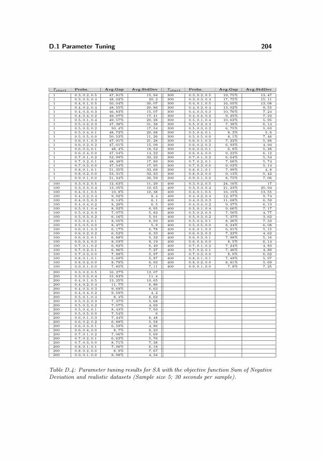
D.1 Parameter Tuning 204
Tstart Probs. Avg.Gap Avg.StdDev Tstart Probs. Avg.Gap Avg.StdDev
1 0.3, 0.2, 0.5 47, 81% 15, 94 300 0.3, 0.2, 0.5 19, 75% 13, 471 0.3, 0.3, 0.4 48, 02% 20, 2 300 0.3, 0.3, 0.4 17, 75% 15, 111 0.4, 0.1, 0.5 50, 04% 30, 07 300 0.4, 0.1, 0.5 16, 05% 13, 081 0.4, 0.2, 0.4 48, 55% 20, 86 300 0.4, 0.2, 0.4 13, 02% 9, 551 0.4, 0.3, 0.3 46, 83% 15, 07 300 0.4, 0.3, 0.3 10, 76% 7, 241 0.4, 0.4, 0.2 49, 07% 17, 41 300 0.4, 0.4, 0.2 9, 25% 7, 231 0.5, 0.1, 0.4 49, 57% 20, 28 300 0.5, 0.1, 0.4 10, 62% 5, 951 0.5, 0.2, 0.3 47, 38% 31, 38 300 0.5, 0.2, 0.3 7, 38% 6, 141 0.5, 0.3, 0.2 50, 4% 17, 54 300 0.5, 0.3, 0.2 6, 75% 5, 631 0.5, 0.4, 0.1 48, 72% 20, 98 300 0.5, 0.4, 0.1 8, 3% 5, 61 0.5, 0.5, 0.0 50, 53% 11, 26 300 0.5, 0.5, 0.0 8, 1% 7, 461 0.6, 0.1, 0.3 47, 91% 21, 28 300 0.6, 0.1, 0.3 7, 22% 5, 881 0.6, 0.2, 0.2 47, 01% 15, 09 300 0.6, 0.2, 0.2 6, 93% 4, 941 0.6, 0.3, 0.1 48, 4% 18, 52 300 0.6, 0.3, 0.1 6, 8% 5, 281 0.6, 0.4, 0.0 47, 04% 14, 22 300 0.6, 0.4, 0.0 9, 22% 6, 121 0.7, 0.1, 0.2 52, 99% 32, 22 300 0.7, 0.1, 0.2 6, 64% 5, 541 0.7, 0.2, 0.1 48, 48% 17, 89 300 0.7, 0.2, 0.1 7, 66% 5, 741 0.7, 0.3, 0.0 47, 54% 17, 95 300 0.7, 0.3, 0.0 9, 03% 5, 141 0.8, 0.1, 0.1 51, 35% 33, 69 300 0.8, 0.1, 0.1 7, 99% 4, 81 0.8, 0.2, 0.0 53, 31% 32, 23 300 0.8, 0.2, 0.0 9, 13% 5, 421 0.9, 0.1, 0.0 51, 34% 30, 59 300 0.9, 0.1, 0.0 8, 75% 7, 06
100 0.3, 0.2, 0.5 12, 63% 11, 29 400 0.3, 0.2, 0.5 24, 16% 17100 0.3, 0.3, 0.4 13, 05% 10, 65 400 0.3, 0.3, 0.4 21, 23% 20, 94100 0.4, 0.1, 0.5 10, 8% 10, 38 400 0.4, 0.1, 0.5 16, 15% 13, 55100 0.4, 0.2, 0.4 9, 92% 8, 4 400 0.4, 0.2, 0.4 12, 97% 9, 74100 0.4, 0.3, 0.3 9, 14% 6, 1 400 0.4, 0.3, 0.3 11, 68% 6, 59100 0.4, 0.4, 0.2 8, 29% 6, 5 400 0.4, 0.4, 0.2 9, 37% 6, 13100 0.5, 0.1, 0.4 8, 92% 6, 95 400 0.5, 0.1, 0.4 9, 66% 7, 17100 0.5, 0.2, 0.3 7, 07% 5, 82 400 0.5, 0.2, 0.3 7, 56% 4, 77100 0.5, 0.3, 0.2 6, 16% 5, 91 400 0.5, 0.3, 0.2 7, 37% 3, 62100 0.5, 0.4, 0.1 8, 05% 6, 93 400 0.5, 0.4, 0.1 8, 26% 7, 33100 0.5, 0.5, 0.0 8, 47% 5, 9 400 0.5, 0.5, 0.0 8, 24% 6, 08100 0.6, 0.1, 0.3 6, 17% 6, 78 400 0.6, 0.1, 0.3 6, 91% 5, 15100 0.6, 0.2, 0.2 6, 52% 6, 33 400 0.6, 0.2, 0.2 7, 22% 4, 62100 0.6, 0.3, 0.1 6, 88% 5, 32 400 0.6, 0.3, 0.1 7, 98% 5, 16100 0.6, 0.4, 0.0 8, 03% 8, 19 400 0.6, 0.4, 0.0 8, 5% 6, 14100 0.7, 0.1, 0.2 6, 82% 6, 49 400 0.7, 0.1, 0.2 7, 24% 4, 83100 0.7, 0.2, 0.1 6, 86% 7, 27 400 0.7, 0.2, 0.1 7, 46% 4, 89100 0.7, 0.3, 0.0 7, 88% 5, 97 400 0.7, 0.3, 0.0 8, 9% 6, 62100 0.8, 0.1, 0.1 5, 69% 5, 87 400 0.8, 0.1, 0.1 7, 49% 5, 97100 0.8, 0.2, 0.0 8, 79% 6, 93 400 0.8, 0.2, 0.0 8, 81% 5, 69100 0.9, 0.1, 0.0 7, 85% 7, 11 400 0.9, 0.1, 0.0 7, 8% 7, 25
200 0.3, 0.2, 0.5 16, 27% 12, 07200 0.3, 0.3, 0.4 15, 83% 11, 4200 0.4, 0.1, 0.5 13, 25% 10, 65200 0.4, 0.2, 0.4 11, 7% 6, 86200 0.4, 0.3, 0.3 9, 69% 6, 63200 0.4, 0.4, 0.2 9, 59% 4, 2200 0.5, 0.1, 0.4 8, 4% 6, 62200 0.5, 0.2, 0.3 7, 37% 5, 68200 0.5, 0.3, 0.2 7, 07% 4, 69200 0.5, 0.4, 0.1 8, 43% 7, 93200 0.5, 0.5, 0.0 7, 54% 6200 0.6, 0.1, 0.3 7, 44% 6, 48200 0.6, 0.2, 0.2 6, 88% 5, 58200 0.6, 0.3, 0.1 6, 59% 4, 86200 0.6, 0.4, 0.0 8, 7% 6, 23200 0.7, 0.1, 0.2 7, 06% 5, 69200 0.7, 0.2, 0.1 6, 63% 5, 76200 0.7, 0.3, 0.0 8, 71% 7, 38200 0.8, 0.1, 0.1 7, 06% 6, 18200 0.8, 0.2, 0.0 8, 9% 7, 67200 0.9, 0.1, 0.0 8, 98% 4, 34
Table D.4: Parameter tuning results for SA with the objective function Sum of NegativeDeviation and realistic datasets (Sample size 5; 30 seconds per sample).

D.1 Parameter Tuning 205
Tstart Probs. Avg.Gap Avg.StdDev Tstart Probs. Avg.Gap Avg.StdDev
1 0.3, 0.2, 0.5 3676, 67% 16, 88 300 0.3, 0.2, 0.5 1563, 33% 4, 161 0.3, 0.3, 0.4 4140% 16, 28 300 0.3, 0.3, 0.4 803, 33% 4, 291 0.4, 0.1, 0.5 3600% 13, 62 300 0.4, 0.1, 0.5 180% 1, 441 0.4, 0.2, 0.4 3566, 67% 12, 26 300 0.4, 0.2, 0.4 50% 0, 571 0.4, 0.3, 0.3 3766, 67% 17, 12 300 0.4, 0.3, 0.3 26, 67% 0, 441 0.4, 0.4, 0.2 3973, 33% 11, 4 300 0.4, 0.4, 0.2 26, 67% 0, 261 0.5, 0.1, 0.4 4463, 33% 11, 39 300 0.5, 0.1, 0.4 40% 0, 441 0.5, 0.2, 0.3 4316, 67% 14, 77 300 0.5, 0.2, 0.3 33, 33% 0, 371 0.5, 0.3, 0.2 4593, 33% 10, 1 300 0.5, 0.3, 0.2 43, 33% 0, 31 0.5, 0.4, 0.1 4950% 12, 7 300 0.5, 0.4, 0.1 96, 67% 0, 711 0.5, 0.5, 0.0 4616, 67% 14, 84 300 0.5, 0.5, 0.0 80% 0, 31 0.6, 0.1, 0.3 4783, 33% 12, 13 300 0.6, 0.1, 0.3 66, 67% 0, 461 0.6, 0.2, 0.2 4666, 67% 19, 57 300 0.6, 0.2, 0.2 70% 0, 531 0.6, 0.3, 0.1 4830% 15, 68 300 0.6, 0.3, 0.1 80% 0, 311 0.6, 0.4, 0.0 5286, 67% 14, 8 300 0.6, 0.4, 0.0 106, 67% 0, 831 0.7, 0.1, 0.2 4636, 67% 11, 19 300 0.7, 0.1, 0.2 46, 67% 0, 341 0.7, 0.2, 0.1 4906, 67% 10, 33 300 0.7, 0.2, 0.1 80% 0, 481 0.7, 0.3, 0.0 4643, 33% 16, 45 300 0.7, 0.3, 0.0 86, 67% 0, 811 0.8, 0.1, 0.1 5110% 15, 69 300 0.8, 0.1, 0.1 96, 67% 0, 281 0.8, 0.2, 0.0 5326, 67% 11, 58 300 0.8, 0.2, 0.0 140% 0, 991 0.9, 0.1, 0.0 5736, 67% 8, 24 300 0.9, 0.1, 0.0 150% 0, 64
100 0.3, 0.2, 0.5 36, 67% 0, 47 400 0.3, 0.2, 0.5 2266, 67% 5, 79100 0.3, 0.3, 0.4 53, 33% 0, 68 400 0.3, 0.3, 0.4 1506, 67% 4, 49100 0.4, 0.1, 0.5 40% 0, 49 400 0.4, 0.1, 0.5 260% 2, 18100 0.4, 0.2, 0.4 26, 67% 0, 39 400 0.4, 0.2, 0.4 96, 67% 1, 16100 0.4, 0.3, 0.3 26, 67% 0, 35 400 0.4, 0.3, 0.3 26, 67% 0, 34100 0.4, 0.4, 0.2 13, 33% 0, 24 400 0.4, 0.4, 0.2 20% 0, 31100 0.5, 0.1, 0.4 30% 0, 37 400 0.5, 0.1, 0.4 50% 0, 44100 0.5, 0.2, 0.3 10% 0, 17 400 0.5, 0.2, 0.3 16, 67% 0, 37100 0.5, 0.3, 0.2 16, 67% 0, 24 400 0.5, 0.3, 0.2 33, 33% 0, 24100 0.5, 0.4, 0.1 73, 33% 0, 43 400 0.5, 0.4, 0.1 106, 67% 0, 53100 0.5, 0.5, 0.0 90% 0, 5 400 0.5, 0.5, 0.0 103, 33% 0, 71100 0.6, 0.1, 0.3 23, 33% 0, 23 400 0.6, 0.1, 0.3 76, 67% 0, 19100 0.6, 0.2, 0.2 33, 33% 0, 31 400 0.6, 0.2, 0.2 50% 0, 45100 0.6, 0.3, 0.1 56, 67% 0, 43 400 0.6, 0.3, 0.1 70% 0, 72100 0.6, 0.4, 0.0 90% 0, 76 400 0.6, 0.4, 0.0 150% 0, 86100 0.7, 0.1, 0.2 53, 33% 0, 23 400 0.7, 0.1, 0.2 86, 67% 0, 37100 0.7, 0.2, 0.1 76, 67% 0, 33 400 0.7, 0.2, 0.1 83, 33% 0, 39100 0.7, 0.3, 0.0 100% 0, 77 400 0.7, 0.3, 0.0 106, 67% 0, 56100 0.8, 0.1, 0.1 63, 33% 0, 37 400 0.8, 0.1, 0.1 90% 0, 53100 0.8, 0.2, 0.0 130% 0, 54 400 0.8, 0.2, 0.0 140% 0, 49100 0.9, 0.1, 0.0 140% 0, 83 400 0.9, 0.1, 0.0 173, 33% 0, 83
200 0.3, 0.2, 0.5 536, 67% 1, 85200 0.3, 0.3, 0.4 103, 33% 0, 97200 0.4, 0.1, 0.5 96, 67% 0, 84200 0.4, 0.2, 0.4 43, 33% 0, 63200 0.4, 0.3, 0.3 10% 0, 09200 0.4, 0.4, 0.2 56, 67% 0, 49200 0.5, 0.1, 0.4 30% 0, 43200 0.5, 0.2, 0.3 30% 0, 37200 0.5, 0.3, 0.2 43, 33% 0, 4200 0.5, 0.4, 0.1 76, 67% 0, 45200 0.5, 0.5, 0.0 120% 0, 46200 0.6, 0.1, 0.3 33, 33% 0, 31200 0.6, 0.2, 0.2 46, 67% 0, 27200 0.6, 0.3, 0.1 60% 0, 49200 0.6, 0.4, 0.0 93, 33% 0, 83200 0.7, 0.1, 0.2 66, 67% 0, 52200 0.7, 0.2, 0.1 56, 67% 0, 52200 0.7, 0.3, 0.0 123, 33% 0, 41200 0.8, 0.1, 0.1 80% 0, 39200 0.8, 0.2, 0.0 120% 0, 77200 0.9, 0.1, 0.0 143, 33% 0, 56
Table D.5: Parameter tuning results for SA with the objective function Sum of NegativeDeviation and generated datasets (Sample size 5; 30 seconds per sample).

D.1 Parameter Tuning 206
Tstart Probs. Avg.Gap Avg.StdDev Tstart Probs. Avg.Gap Avg.StdDev
1 0.3, 0.2, 0.5 35, 99% 1, 13 300 0.3, 0.2, 0.5 164, 3% 1, 031 0.3, 0.3, 0.4 23, 69% 1, 14 300 0.3, 0.3, 0.4 144, 67% 0, 931 0.4, 0.1, 0.5 6, 1% 0, 17 300 0.4, 0.1, 0.5 106, 08% 1, 291 0.4, 0.2, 0.4 6, 7% 0, 25 300 0.4, 0.2, 0.4 22, 59% 0, 431 0.4, 0.3, 0.3 7, 33% 0, 18 300 0.4, 0.3, 0.3 10, 94% 0, 251 0.4, 0.4, 0.2 7, 53% 0, 25 300 0.4, 0.4, 0.2 11, 24% 0, 341 0.5, 0.1, 0.4 7, 1% 0, 17 300 0.5, 0.1, 0.4 10, 01% 0, 121 0.5, 0.2, 0.3 7, 74% 0, 26 300 0.5, 0.2, 0.3 9, 68% 0, 191 0.5, 0.3, 0.2 8, 04% 0, 26 300 0.5, 0.3, 0.2 9, 02% 0, 241 0.5, 0.4, 0.1 8, 9% 0, 33 300 0.5, 0.4, 0.1 13, 41% 0, 321 0.5, 0.5, 0.0 9, 82% 0, 33 300 0.5, 0.5, 0.0 14, 55% 0, 321 0.6, 0.1, 0.3 8, 01% 0, 26 300 0.6, 0.1, 0.3 9, 91% 0, 111 0.6, 0.2, 0.2 9, 37% 0, 32 300 0.6, 0.2, 0.2 10, 79% 0, 241 0.6, 0.3, 0.1 9, 4% 0, 43 300 0.6, 0.3, 0.1 12, 43% 0, 291 0.6, 0.4, 0.0 9, 88% 0, 37 300 0.6, 0.4, 0.0 13, 89% 0, 321 0.7, 0.1, 0.2 8, 18% 0, 39 300 0.7, 0.1, 0.2 11, 07% 0, 241 0.7, 0.2, 0.1 9, 6% 0, 42 300 0.7, 0.2, 0.1 12, 65% 0, 251 0.7, 0.3, 0.0 12, 25% 0, 36 300 0.7, 0.3, 0.0 17, 08% 0, 111 0.8, 0.1, 0.1 9, 27% 0, 26 300 0.8, 0.1, 0.1 12, 91% 0, 371 0.8, 0.2, 0.0 11, 58% 0, 29 300 0.8, 0.2, 0.0 16, 46% 0, 241 0.9, 0.1, 0.0 13, 02% 0, 37 300 0.9, 0.1, 0.0 15, 51% 0, 32
100 0.3, 0.2, 0.5 140, 05% 0, 76 400 0.3, 0.2, 0.5 165, 33% 1, 1100 0.3, 0.3, 0.4 118, 42% 1, 09 400 0.3, 0.3, 0.4 146, 1% 0, 91100 0.4, 0.1, 0.5 67, 35% 1, 32 400 0.4, 0.1, 0.5 111, 62% 1, 05100 0.4, 0.2, 0.4 18, 56% 0, 46 400 0.4, 0.2, 0.4 26, 57% 0, 46100 0.4, 0.3, 0.3 10, 93% 0, 19 400 0.4, 0.3, 0.3 12, 49% 0, 26100 0.4, 0.4, 0.2 9, 7% 0, 12 400 0.4, 0.4, 0.2 10, 09% 0, 14100 0.5, 0.1, 0.4 10, 24% 0, 14 400 0.5, 0.1, 0.4 11, 61% 0, 26100 0.5, 0.2, 0.3 9, 34% 0, 12 400 0.5, 0.2, 0.3 9, 06% 0, 18100 0.5, 0.3, 0.2 10, 63% 0, 11 400 0.5, 0.3, 0.2 10, 32% 0, 12100 0.5, 0.4, 0.1 13, 51% 0, 25 400 0.5, 0.4, 0.1 14, 68% 0, 26100 0.5, 0.5, 0.0 13, 51% 0, 25 400 0.5, 0.5, 0.0 13, 34% 0, 18100 0.6, 0.1, 0.3 11, 21% 0, 21 400 0.6, 0.1, 0.3 10, 7% 0, 29100 0.6, 0.2, 0.2 10, 66% 0, 22 400 0.6, 0.2, 0.2 12, 52% 0, 14100 0.6, 0.3, 0.1 13, 25% 0, 24 400 0.6, 0.3, 0.1 11, 4% 0, 17100 0.6, 0.4, 0.0 14, 98% 0, 3 400 0.6, 0.4, 0.0 15, 3% 0, 26100 0.7, 0.1, 0.2 11, 38% 0, 25 400 0.7, 0.1, 0.2 10, 62% 0, 22100 0.7, 0.2, 0.1 12, 81% 0, 18 400 0.7, 0.2, 0.1 15, 13% 0, 32100 0.7, 0.3, 0.0 15, 41% 0, 18 400 0.7, 0.3, 0.0 15, 22% 0, 19100 0.8, 0.1, 0.1 14, 67% 0, 25 400 0.8, 0.1, 0.1 13, 38% 0, 18100 0.8, 0.2, 0.0 17, 35% 0, 29 400 0.8, 0.2, 0.0 17, 02% 0, 19100 0.9, 0.1, 0.0 16, 43% 0, 24 400 0.9, 0.1, 0.0 17, 12% 0, 12
200 0.3, 0.2, 0.5 149, 02% 0, 72200 0.3, 0.3, 0.4 129, 62% 1, 1200 0.4, 0.1, 0.5 93, 24% 1, 25200 0.4, 0.2, 0.4 22, 35% 0, 43200 0.4, 0.3, 0.3 11, 75% 0, 3200 0.4, 0.4, 0.2 11, 79% 0, 36200 0.5, 0.1, 0.4 10, 33% 0, 11200 0.5, 0.2, 0.3 8, 99% 0, 22200 0.5, 0.3, 0.2 11, 33% 0, 12200 0.5, 0.4, 0.1 11, 41% 0, 18200 0.5, 0.5, 0.0 14, 82% 0, 24200 0.6, 0.1, 0.3 9, 6% 0, 3200 0.6, 0.2, 0.2 11, 96% 0, 25200 0.6, 0.3, 0.1 11, 14% 0, 11200 0.6, 0.4, 0.0 12, 88% 0, 24200 0.7, 0.1, 0.2 12, 21% 0, 3200 0.7, 0.2, 0.1 13, 12% 0, 26200 0.7, 0.3, 0.0 15, 84% 0, 21200 0.8, 0.1, 0.1 14% 0, 36200 0.8, 0.2, 0.0 14, 61% 0, 3200 0.9, 0.1, 0.0 18, 27% 0, 12
Table D.6: Parameter tuning results for SA with the objective function Largest NegativeDeviation and realistic datasets (Sample size 5; 30 seconds per sample).
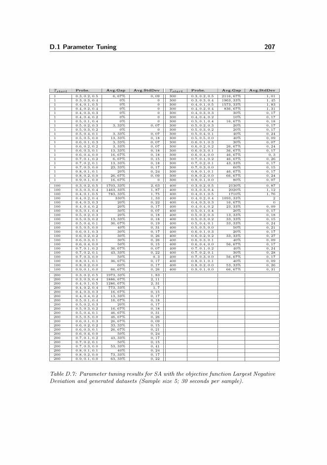
D.1 Parameter Tuning 207
Tstart Probs. Avg.Gap Avg.StdDev Tstart Probs. Avg.Gap Avg.StdDev
1 0.3, 0.2, 0.5 6, 67% 0, 09 300 0.3, 0.2, 0.5 2116, 67% 1, 011 0.3, 0.3, 0.4 0% 0 300 0.3, 0.3, 0.4 1963, 33% 1, 451 0.4, 0.1, 0.5 0% 0 300 0.4, 0.1, 0.5 1573, 33% 1, 831 0.4, 0.2, 0.4 0% 0 300 0.4, 0.2, 0.4 836, 67% 1, 311 0.4, 0.3, 0.3 0% 0 300 0.4, 0.3, 0.3 30% 0, 171 0.4, 0.4, 0.2 0% 0 300 0.4, 0.4, 0.2 10% 0, 171 0.5, 0.1, 0.4 0% 0 300 0.5, 0.1, 0.4 16, 67% 0, 181 0.5, 0.2, 0.3 3, 33% 0, 07 300 0.5, 0.2, 0.3 20% 0, 171 0.5, 0.3, 0.2 0% 0 300 0.5, 0.3, 0.2 20% 0, 171 0.5, 0.4, 0.1 3, 33% 0, 07 300 0.5, 0.4, 0.1 40% 0, 241 0.5, 0.5, 0.0 13, 33% 0, 18 300 0.5, 0.5, 0.0 40% 0, 091 0.6, 0.1, 0.3 3, 33% 0, 07 300 0.6, 0.1, 0.3 30% 0, 071 0.6, 0.2, 0.2 3, 33% 0, 07 300 0.6, 0.2, 0.2 26, 67% 0, 241 0.6, 0.3, 0.1 13, 33% 0, 18 300 0.6, 0.3, 0.1 36, 67% 0, 171 0.6, 0.4, 0.0 16, 67% 0, 18 300 0.6, 0.4, 0.0 46, 67% 0, 31 0.7, 0.1, 0.2 6, 67% 0, 15 300 0.7, 0.1, 0.2 46, 67% 0, 261 0.7, 0.2, 0.1 13, 33% 0, 18 300 0.7, 0.2, 0.1 43, 33% 0, 171 0.7, 0.3, 0.0 23, 33% 0, 17 300 0.7, 0.3, 0.0 60% 0, 151 0.8, 0.1, 0.1 20% 0, 24 300 0.8, 0.1, 0.1 46, 67% 0, 171 0.8, 0.2, 0.0 26, 67% 0, 09 300 0.8, 0.2, 0.0 66, 67% 0, 241 0.9, 0.1, 0.0 16, 67% 0 300 0.9, 0.1, 0.0 80% 0, 07
100 0.3, 0.2, 0.5 1703, 33% 2, 63 400 0.3, 0.2, 0.5 2130% 0, 87100 0.3, 0.3, 0.4 1463, 33% 1, 87 400 0.3, 0.3, 0.4 2020% 1, 12100 0.4, 0.1, 0.5 783, 33% 1, 75 400 0.4, 0.1, 0.5 1710% 1, 76100 0.4, 0.2, 0.4 330% 1, 33 400 0.4, 0.2, 0.4 1093, 33% 2100 0.4, 0.3, 0.3 20% 0, 22 400 0.4, 0.3, 0.3 16, 67% 0100 0.4, 0.4, 0.2 20% 0, 17 400 0.4, 0.4, 0.2 23, 33% 0, 09100 0.5, 0.1, 0.4 30% 0, 07 400 0.5, 0.1, 0.4 20% 0, 17100 0.5, 0.2, 0.3 20% 0, 18 400 0.5, 0.2, 0.3 13, 33% 0, 18100 0.5, 0.3, 0.2 13, 33% 0, 18 400 0.5, 0.3, 0.2 33, 33% 0, 15100 0.5, 0.4, 0.1 36, 67% 0, 19 400 0.5, 0.4, 0.1 33, 33% 0, 24100 0.5, 0.5, 0.0 40% 0, 31 400 0.5, 0.5, 0.0 50% 0, 21100 0.6, 0.1, 0.3 30% 0, 17 400 0.6, 0.1, 0.3 20% 0, 17100 0.6, 0.2, 0.2 30% 0, 26 400 0.6, 0.2, 0.2 33, 33% 0, 27100 0.6, 0.3, 0.1 30% 0, 26 400 0.6, 0.3, 0.1 40% 0, 09100 0.6, 0.4, 0.0 50% 0, 15 400 0.6, 0.4, 0.0 56, 67% 0, 17100 0.7, 0.1, 0.2 36, 67% 0, 07 400 0.7, 0.1, 0.2 40% 0, 24100 0.7, 0.2, 0.1 43, 33% 0, 22 400 0.7, 0.2, 0.1 30% 0, 28100 0.7, 0.3, 0.0 50% 0, 3 400 0.7, 0.3, 0.0 56, 67% 0, 17100 0.8, 0.1, 0.1 36, 67% 0, 17 400 0.8, 0.1, 0.1 40% 0, 09100 0.8, 0.2, 0.0 60% 0, 17 400 0.8, 0.2, 0.0 53, 33% 0, 26100 0.9, 0.1, 0.0 66, 67% 0, 26 400 0.9, 0.1, 0.0 66, 67% 0, 31
200 0.3, 0.2, 0.5 1973, 33% 1, 83200 0.3, 0.3, 0.4 1886, 67% 2, 11200 0.4, 0.1, 0.5 1286, 67% 2, 31200 0.4, 0.2, 0.4 773, 33% 1, 7200 0.4, 0.3, 0.3 16, 67% 0, 15200 0.4, 0.4, 0.2 13, 33% 0, 17200 0.5, 0.1, 0.4 16, 67% 0, 18200 0.5, 0.2, 0.3 20% 0, 17200 0.5, 0.3, 0.2 16, 67% 0, 18200 0.5, 0.4, 0.1 46, 67% 0, 31200 0.5, 0.5, 0.0 46, 67% 0, 26200 0.6, 0.1, 0.3 26, 67% 0, 09200 0.6, 0.2, 0.2 33, 33% 0, 15200 0.6, 0.3, 0.1 26, 67% 0, 21200 0.6, 0.4, 0.0 50% 0, 24200 0.7, 0.1, 0.2 43, 33% 0, 17200 0.7, 0.2, 0.1 50% 0, 15200 0.7, 0.3, 0.0 53, 33% 0, 41200 0.8, 0.1, 0.1 40% 0, 24200 0.8, 0.2, 0.0 73, 33% 0, 17200 0.9, 0.1, 0.0 63, 33% 0, 22
Table D.7: Parameter tuning results for SA with the objective function Largest NegativeDeviation and generated datasets (Sample size 5; 30 seconds per sample).

Appendix E
Column Matheuristic - Tuningand Testing
E.1 Parameter Tuning
E.1.1 Summary

E.1 Parameter Tuning 209
PTD SoND LNDDataset Demand z σ z∗ z σ z∗ z σ z∗
Realistic datasets:
Tune2007-01 Normal 523.2 5 530.5 201.2 3.9 197 6 0 6Tune2007-01 Peak 524.6 2.3 527.5 234.6 5.7 226 7 0 7Tune2007-02 Normal 562.2 1.4 563.5 55.8 10.6 42 3.6 0.5 3Tune2007-02 Peak 564.8 1.4 567 78 9.4 63 3.8 0.4 3Tune2007-12 Normal 624.5 3.1 628 561.8 6.8 551 12.4 0.5 12Tune2007-12 Peak 622.8 2.7 626.5 624.6 4 618 13 0 13Tune2008-01 Normal 695.4 2.3 697 443.6 5.3 438 10.2 0.4 10Tune2008-01 Peak 696.9 4.6 702.5 495.6 7.6 488 11 0 11
σ 2.9 6.7 0.2
Generated datasets:
TuneEmpty Normal 1145.2 28.7 1209 0.0 0.0 0 0.0 0.0 0TuneEmpty Peak 1137.8 31.7 1200.5 0.0 0.0 0 0.0 0.0 0TuneSparse1 Normal 674.8 70.5 820.5 0.0 0.0 0 0.0 0.0 0TuneSparse2 Peak 728.2 99.5 809 0.0 0.0 0 0.0 0.0 0TuneSparse2 Normal 621.6 37.1 744.5 0.0 0.0 0 0.0 0.0 0TuneSparse2 Peak 715.2 68.1 753.5 0.2 0.4 0 0.4 0.5 0
σ 55.9 0.1 0.1
Table E.1: Summary of tuning for the best parameter settings for Column Matheuristic.Overview of average found solutions z, standard deviations σ and best found solutionsz∗ with SA for the three objective functions Paired Tour Days (PTD), Sum of NegativeDeviation (SoND) and Largest Negative Deviation (LND) over all tuning datasets.Average standard deviation σ is also calculated.
PTD Realistic Generatedcmax z σ z σ
400 5.36% 6.60 14.35% 68.62600 2.48% 4.61 9.97% 55.94800 0.59% 2.85 10.38% 59.17
SoND Realistic Generatedcmax z σ z σ
400 27.76% 7.56 0.10 0.22600 13.84% 5.90 0.03 0.07800 8.56% 6.67 0.03 0.07
LND Realistic Generatedcmax z σ z σ
400 17.75% 0.25 0.17 0.18600 11.89% 0.34 0.07 0.09800 6.50% 0.25 0.27 0.15
Table E.2: Results of tuning for the parameter setting for Column Matheuristic.Overview of average percentage gap (or average of averages) z and standard deviationsσ for the three objective functions Paired Tour Days (PTD), Sum of Negative Deviation(SoND) and Largest Negative Deviation (LND) over all tuning datasets. These resultsare illustrated in figure 9.10, 9.11 and 9.12 on pages 144 to 144.

Appendix F
Comparison of SolutionApproaches
F.1 Comparison of Simulated Annealing againstColumn Matheuristic

F.1 Comparison of Simulated Annealing against Column Matheuristic 211
Objective: SoND Simulated Column CMH improves SAAnnealing Matheuristic (% improvement)
Dataset Demand z σ z∗ z σ z∗ z σ z∗
Realistic datasets:
Test2007-03 Normal 594.2 89.1 449.0 357.7 13.5 344.0 39.8% 84.8% 23.4%Test2007-03 Peak 662.2 39.8 591.0 388.3 11.5 377.0 41.4% 71.1% 36.2%Test2007-04 Normal 429.6 26.9 382.0 202.3 10.1 193.0 52.9% 62.6% 49.5%Test2007-04 Peak 494.0 4.5 486.0 233.7 13.3 225.0 52.7% -197.8% 53.7%Test2008-02 Normal 692.6 64.5 637.0 525.0 4.6 521.0 24.2% 92.9% 18.2%Test2008-02 Peak 726.0 24.7 704.0 580.3 5.7 574.0 20.1% 77.0% 18.5%Test2008-03 Normal 408.6 71.3 302.0 180.0 11.3 173.0 55.9% 84.2% 42.7%Test2008-03 Peak 513.6 65.2 407.0 237.0 10.8 228.0 53.9% 83.4% 44.0%
Averages 48.3 10.1 42.6% 44.8% 35.8%
Generated datasets:
TestEmpty Normal 7.8 4.0 3.0 0.0 0.0 0.0 100.0% 100.0% 100.0%TestEmpty Peak 18.0 5.7 9.0 0.0 0.0 0.0 100.0% 100.0% 100.0%TestSparse1 Normal 85.0 53.0 12.0 0.0 0.0 0.0 100.0% 100.0% 100.0%TestSparse1 Peak 84.4 11.4 68.0 9.7 6.7 4.0 88.5% 41.4% 94.1%TestSparse2 Normal 390.0 0.0 390.0 344.7 12.6 333.0 11.6% - 14.6%TestSparse2 Peak 464.0 0.0 464.0 371.7 31.9 335.0 19.9% - 27.8%
Averages 12.3 8.5 70.0% 85.4% 72.8%
Table F.1: Comparison of SA and CMH for the objective function SoND. For eachsolution approach is listed the average found solutions z, standard deviations σ andbest found solutions z∗. The comparison columns are the percentage improvement forthe CMH over the SA, i.e. positive numbers denotes improvement (CMH better thanSA) and the negative the opposite.
Objective: LND Simulated Column CMH improves SAAnnealing Matheuristic (% improvement)
Dataset Demand z σ z∗ z σ z∗ z σ z∗
Realistic datasets:
Test2007-03 Normal 10.0 0.0 10.0 9.0 0.0 9.0 10.0% - 10.0%Test2007-03 Peak 10.0 0.0 10.0 9.0 0.0 9.0 10.0% - 10.0%Test2007-04 Normal 6.0 0.0 6.0 4.3 0.6 4.0 27.8% - 33.3%Test2007-04 Peak 6.6 0.5 6.0 5.3 0.6 5.0 19.2% -5.4% 16.7%Test2008-02 Normal 15.6 0.5 15.0 13.7 0.6 13.0 12.4% -5.4% 13.3%Test2008-02 Peak 16.2 0.4 16.0 14.0 0.0 14.0 13.6% 100.0% 12.5%Test2008-03 Normal 7.4 0.5 7.0 6.0 0.0 6.0 18.9% 100.0% 14.3%Test2008-03 Peak 8.0 0.0 8.0 6.0 0.0 6.0 25.0% - 25.0%
Averages 0.3 0.2 17.1% 47.3% 16.9%
Generated datasets:
TestEmpty Normal 0.0 0.0 0.0 0.0 0.0 0.0 - - -TestEmpty Peak 1.0 0.0 1.0 0.7 0.6 0.0 33.3% - 100.0%TestSparse1 Normal 1.0 0.0 1.0 1.0 0.0 1.0 0.0% - 0.0%TestSparse1 Peak 2.2 0.4 2.0 2.7 0.6 2.0 -21.2% -29.1% 0.0%TestSparse2 Normal 4.6 0.5 4.0 4.0 0.0 4.0 13.0% 100.0% 0.0%TestSparse2 Peak 5.4 0.5 5.0 4.0 0.0 4.0 25.9% 100.0% 20.0%
Averages 0.3 0.2 10.2% 57.0% 24.0%
Table F.2: Comparison of SA and CMH for the objective function LND. For eachsolution approach is listed the average found solutions z, standard deviations σ andbest found solutions z∗. The comparison columns are the percentage improvement forthe CMH over the SA, i.e. positive numbers denotes improvement (CMH better thanSA) and the negative the opposite.