romanian reports in physics, vol. 68, supplement, p. s799

Romanian Reports in Physics, Vol. 68, Supplement, P. S799–S845, 2016

GAMMA-BEAM INDUSTRIAL APPLICATIONS AT ELI-NP

G. SULIMAN1, V. IANCU1,*, C.A. UR1, M. IOVEA2, I. DAITO3, H. OHGAKI3

1ELI-NP, ”Horia Hulubei” National Institute for Physics and Nuclear Engineering,30 Reactorului Street, RO-077125, Bucharest-Magurele, Romania

2Accept Pro 2000, Nerva Traian 1, K6, Apt 26, Bucharest, RO-031041, Romania3Institute of Advanced Energy, Kyoto University, Uji, Kyoto 6110011, Japan

∗Corresponding author E-mail: [email protected]

Abstract. An ultra-bright, energy tunable and monochromatic gamma-ray sourcein the range of 0.2–19.5 MeV produced by Laser-Compton Backscattering technique isideal for non-destructive testing applications. Consequently, this source satisfies the cri-teria for large-size product investigations with added capabilities like isotope detectionthrough the use of nuclear resonance fluorescence (NRF) technique. This documentpresents the technical description of two major industrial applications of gamma beamsenvisaged at ELI-NP: industrial applications based on NRF and industrial radioscopyand tomography. Both applications exploit the unique characteristics of the gammabeam to deliver new opportunities for the industry. The non-destructive assay basedon high-brightness gamma rays can be successfully applied for safeguard applicationsand management of radioactive wastes. Radioscopy and computed tomography per-formed at ELI-NP has the potential to achieve high spatial resolution and high contrastsensitivity. The performance of the experimental setups proposed is discussed in de-tail in sections 2.3 and 3.3; the performance figures cited there are based on analyticalcalculations and numerical simulations.

Key words: Nuclear resonance fluorescence, radiography and computed tomog-raphy, high-intensity gamma beams.

1. INTRODUCTION

The White Book of the Extreme Light Infrastructure-Nuclear Physics (ELI-NP) project [1] proposes a series of applications that take advantage of the outstand-ing quality of the gamma beam available at ELI-NP. From the possible applicationsmentioned in the White Book, this Technical Design Report (TDR) describes thepotential experiments that use the brilliant gamma beam for non-destructive investi-gations, such as industrial gamma beam tomography and nuclear resonance fluores-cence (NRF) based applications.

An ultra-bright, energy-tunable and monochromatic gamma-ray source in therange of 0.2–19.5 MeV produced by Laser-Compton Scattering (LCS) technique isideal for the non-destructive testing (NDT) applications. Practically, using this sourceis possible to detect and/or measure nuclides in an object non-destructively, which isa key technology for nuclear industrial applications such as management of radioac-

(c) 2016 RRP 68(Supplement) S799–S845 - v.1.3*2016.5.18 —ATG

S800 G. Suliman et al. 2

tive wastes, nuclear material accounting and safeguards. Moreover, the new sourcecould be a perfect solution for fulfilling all technical requirements for the large-sizeand complex product investigations in aeronautics, automotive, die-cast or sinteredindustries, new materials and technologies development, for archaeological artifactsand work of art objects analysis and many others [1].

The design of the experiments and the estimation of the achievable countingrates and measurement times are highly dependent on the assumed parameters of thebeam delivered by the machine. As a starting point for the estimates in this TDRwe have used the values detailed in the Technical Design Report published by theEuroGammaS collaboration in Ref. [2].

Another version of the parameters of the source is shown on the webpage of theELI-NP project: http://www.eli-np.ro/documents/ELI-NP-GBS-Specifications-rev3-1.pdf. These two documents are in total agreement and the comparison between thevalues significant for the present TDR is explained in the following.

Time-average spectral density at the peak energy versus spectral density[1/(s·eV)]. The range of (0.8–4.0)×104 photons/s·eV is the same in both tables, withthe added benefit that the table in Ref. [2] details the inverse correlation betweenthe energy of the photon beam and the achievable spectral density. This spectralvalue is used in the present TDR for estimating the number of NRF photons beingdetected by the ELI-NP Array of Detectors (ELIADE) array. Table 8 uses for thenumber of incoming photons the value of 50000 ph/s ΓD calculated using 28000ph/s·eV, representing a conservative estimate of the spectral density at 2.1 MeV, (theresonance energy of the uranium line) and 1.78 eV for the width of the resonance.

Number of photons/s within the bandwidth. The number of photons/s com-ing from the source is not present in the table linked from the web page of the project,but it is shown in the TDR of the gamma source [2]. This value can be estimated us-ing the value of the spectral density, the energy of the beam and the bandwidth. Forexample, for a beam of 2 MeV, bandwidth of 0.5% and spectral density of 4×104

ph/s·eV an estimate of the total number of photons can be obtained as:

Photons/s= SpectralDensity×energy× bandwidth=

4×104×5×10−3×2×106 = 4×108photons/s,(1)

which is in agreement with the value shown in Ref. [2]. It should be noted that whilethe spectral density is decreasing by a factor or 5 over the whole energy range, thetotal number of photons/s within the bandwidth increases slightly. These values areused in the present TDR for estimating the background in NRF experiments and alsoin estimating the measurement time needed in the tomography setup. In some caseswe have used a conservative value of 108 photons/s, or where it was the case, a valueof 106 photons/macrobunch, derived from this value.


3 Gamma-beam industrial applications at ELI-NP S801

2. INDUSTRIAL APPLICATIONS BASED ON NRF

2.1. INTRODUCTION

The nuclear resonance fluorescence (NRF) is an attractive non-destructive anal-ysis method because it provides signatures for a wide variety of materials, signaturesthat can be used to characterize the irradiated samples. Its use for detecting spe-cial nuclear materials within cargo containers was proposed by Bertozzi et al. [3]and subsequently developed by several organizations like Passport Systems, Inc.,Pacific Northwest National Laboratory (PNNL) and Lawrence Livermore NationalLaboratory (LLNL) which have explored various research issues related to appli-cations based on NRF [5–8]. The Department of Energy, USA, commissioned areport [4], which investigated the possible applications of NRF and the associatedresearch challenges. The topics identified are mostly related to special nuclear mate-rials (SNM) and nuclear safeguards applications such as U enrichment confirmationof UF6 canisters, geo-sourcing of material, weapons dismantlement verification, di-rect measurement of Pu in spent fuel, analysis of gas samples, characterization ofsuspect material, and verification of SNM in a cargo container [4]. These topics wereextensively studied in recent years using mostly continuous Bremsstrahlung sourcesand only few LCS sources [5–14].

Apart from SNM and nuclear safeguards applications, NRF-based applicationsfor chemical compounds and organic materials have been proposed and demonstratedrecently. Hayakawa et al. [12] demonstrated the non-destructive inspection of ashielded explosive by using NRF measurement, and succeeded to extract the abun-dance ratio of chemical components, 12C/14N, of melamine compound. Beck et al.[15] used NRF to determine the 13C content in diamond in concentrations as smallas 0.5 mg, confirming the results of Raman scattering while demonstrating the feasi-bility of identifying mg quantities in a target. In the future, non-destructive measure-ments of heavy element contaminates in foods can also be envisaged. The maximumconcentrations of the heavy metal contaminates in food established by Codex [16] arein the range of 0.1 mg/kg up to 200 mg/kg, well within the range of NRF methods.

As noted above, the applicability of the NRF method is quite general and broad.Moreover, the NRF method can be used in conjunction with tomography to produceelemental maps in objects of various compositions [17–20]. Lakshmanan et al. in aMonte Carlo simulations study proposed to use NRF imaging for visualizing breastcancer lesions [17]. Recently a 2D-image of isotope distribution of 208Pb was demon-strated by using NRF by Toyokawa et al. [18]. In contrast to other nuclear methodsused for composition analysis (activation analysis, elastic recoil analysis, accelera-tor mass spectroscopy) NRF requires very limited manipulation of the materials anddoes not noticeably affect the investigated objects. This, in turn, extends the potentialuses of NRF methods to characterizing the internal structure of valuable objects like



historical artifacts, archeological objects, and works of art.The two detection schemes used for NRF-based investigations are the scatter-

ing and the transmission method. In both cases interrogating photons are used toinduce the resonant absorption while the de-excitation photons are detected eitherin a backscattering geometry or in a self-absorption (transmission) geometry [21].The applications described here take in consideration both measuring schemes. Asa result, the present TDR will propose two experimental setups at ELI-NP, one foreach of the measurements schemes. The detailed description and rate estimates forthe many of the possible applications are challenging due to the lack of informationconcerning the cross section and level widths of the nuclei of interest. As a result,measurements aimed at improving the quality of the NRF measurements for appli-cations will also be a part of the experimental efforts proposed to be carried out atELI-NP.

2.2. METHODS

2.2.1. Scattering NRF measurements

The general setup employed in the scattering NRF experiments is illustrated inFig. 1. Here the investigated object is placed in the beam and the resonant photonsare detected in a backscattered geometry by a detector located off-beam. Except theresonant photons, all other scattered photons have low energy due to the nature ofCompton scattering. Therefore the high-energy resonant photons should be easilydistinguished.

Fig. 1 – Schematic view of the backscattering NRF setup.

Hagmann et al. [5] performed Monte Carlo simulations for such geometry at aγ-ray flux of 1013 /s, which corresponds to a spectral density of flux of 1010 /s/keV.



They concluded that using NRF with these source parameters would allow detectionof low concentration of U-238, 1 Bq/g, in a practical measurement time of 100 s [5].The future gamma source from ELI-NP is expected to be a few orders of magnitudelower in intensity, which would mean that measuring higher concentrations could beachieved in still practical experimental times of a few hours.

2.2.2. Transmission NRF measurements using the notch method

The second detection method proposed for NRF measurements is the self-absorption or the transmission method (see Fig. 2) [21]. In this method the object-transmitted gamma beam strikes a sample (witness foil) that contains an isotope ofinterest. Same isotope is expected to exist in the investigated object in smaller con-centrations. The detection of resonant photons scattered by the witness foil is donewith a off-beam detector in a backscattering geometry, often referred to as the “notchdetector”. The flux of the transmitted off-resonance photons may be detected using adetector placed downstream of the witness foil in the beam as pictured in Fig. 2. Col-limators may be used to define the beam and to remove scattered radiation. Contraryto the scattering NRF detection method where the photons that undergo NRF in theobject are registered in the detector, in the transmission method the notch detectormeasures the attenuation of the resonant photons in the witness foil. A preferentialattenuation of the resonant photons in the witness foil would indicate the presence ofthat isotope of interest in the investigated object [9, 21].

Fig. 2 – Schematic view of the transmission NRF setup.

The applicability of the transmission method is limited by the thickness of theinvestigated objects. Ludewigt et al. [9] give an overview of the use of NRF meth-ods for three potential safeguard applications: “the isotopic assay of spend nuclearfuel, the measurement of 235U enrichment in UF6 cylinders and the determination of239Pu in mixed oxide (MOX) fuel”. The main challenge encountered in these appli-cations is obtaining enough statistics to ensure low uncertainties. As an alternative tobremsstrahlung beam, intense quasi-mononenergetic beams with small energy spreadmay be the solution to overcome this challenge. Shorter measurement times couldpotentially be achieved with intense quasi-monoenergetic photon sources like thosedelivered by ELI-NP. Estimation of the expected counting rate by use of transmission



method will be described in section 2.3.3.

2.2.3. Level widths and cross sections in support of NRF applications

The gamma beam at ELI-NP, together with the proposed array of detectorsare the perfect tool for measuring the level widths and the NRF cross sections ofnuclei of interest for applications. The lack of reliable data on the resonances ofmany of the stable or long-lived nuclei precludes the development of a sustainedmeasurement program. For example, in the case of spent nuclear fuel (SNF) it is stillunknown if 240Pu has sufficiently strong resonances to make measurements possible[9]. The situation is the same for most of the other transuranic isotopes. The situationis usually not better for lighter nuclei that could be of interest for the applicationsoutlined in the previous sections. As a result dedicated measurements to accuratelydetermine the resonance cross sections will be performed for most of the isotopes ofinterest.

2.3. FEASIBILITY OF THE PROPOSED METHODS IN ELI-NP CONTEXT

2.3.1. Numerical simulations

One of the main advantages of using the gamma beam at ELI-NP for appli-cations based on NRF is the availability of an advanced detector array, which canenhance by an order of magnitude the advantages coming from the high quality ofthe gamma beam. The proposed ELI-NP Array of Detectors (ELIADE) is made of8 segmented clover detectors similar to those used in the TIGRESS array [22, 23]placed on two rings, one at 98 degrees and another at 135 degrees with respect tothe photon beam direction. The current experimental setup considers the possibilityof having the ring at 98 degrees slightly adjustable, so that it can also be used at 90degrees.

Similar clover detectors are operational at TIGRESS since 2009, and they arealready characterized and fully described in simulations [22, 23]. On one hand, thismakes analytical calculations like those presented in the next section more reliable,as experimental data can be used for comparison. On the other hand, the specificsof the experimental setup at ELI-NP and the particular time structure of the gammabeam need to be taken into account.

Schematic representation of the experimental setup, as it is viewed fromGEANT4 [24, 25] simulations is presented bellow. Figure 3 shows the ELIADEsetup in the configuration that will be used for NRF experiments aimed at discover-ing the NRF signatures of nuclei of interest. This configuration is optimized for veryaccurate measurements, even at the cost of longer experiments: the target can be thin,and the measurements can rely on the segmentation of the detectors to deal with theCompton scattered photons from the target.



Fig. 3 – 3D rendering of the ELIADE setup.

For applications we are interested in obtaining the highest signal/noise ratio andan experimental time as short as possible. In the case of transmission experimentsthis translates into using a much thicker target at the centre of the ELIADE array(notch detector). In the case of scattering experiments, when the object of interestwill be placed at the centre of the array the thickness is fixed by the object to beinvestigated. In both types of experiments we can expect a significant amount ofCompton scattering from the gamma beam on the object in the centre of the arrayto reach the detectors. Assuming that the NRF signature of the nuclei of interest isalready know, to reduce the impact of these events on the pile-up conditions in thedetector we can use a passive lead filter which will have a much higher impact on thelow energy Compton scattered photons than on the high energy NRF photons. Figure4 shows a possible configuration of the ELIADE array where a thick (2 cm) Pb filterseparates each of the detectors from the centre of the array.

The efficiency curves for this type of clover detectors were previously studiedin Ref. [22]. In this study the clovers are used in a configuration using also anti-Compton detectors surrounding the cryostat. The impact of the lead filter on theabsolute photo peak efficiency (assessed using our GEANT4 simulation of the Cloverdetector) and on the peak-to-total ratio using monoenergetic point sources for thehigh energy photons we expect from NRF resonances are shown in Fig. 5.



Fig. 4 – 3D rendering of the ELIADE setup with a thick Pb filter as the red ball object.

Fig. 5 – Performance (absolute efficiency and peak-to-total ratio) for a single segmented cloverdetector.

2.3.2. Analytical description of the background: Compton scattering and pairproduction from the target

The gamma beam of ELI-NP has some very specific characteristics. As a resultof the electron beam structure and laser recirculation time at the interaction point thephotons are emitted in very high intensity and in very short duration pulses. At de-sign parameters, 108 photons are reaching the target each second, which are groupedin 100 macrobunches of 106 photons each. One macrobunch is made of 32 mi-crobunches of a few ps length, separated by 16 ns. Even in the extraordinary band-width conditions of ELI-NP (0.5% of RMS energy), the number of photons within atypical nuclear resonance width (1 eV) is only of the order of 104 ph/s·eV. In theseconditions, it is important to estimate the number of photons being scattered from the



target towards the detectors.The two main processes that generate photons scattered in the target towards

the detectors are the Compton effect and the pair generation in nuclear field. Otherless studied processes like Delbruck, Nuclear Thomson and Nuclear Rayleigh, whichmight become important for certain nuclei, have been ignored in the analysis on thegrounds of their low probability and the fact they were not shown to have a significantimpact in previous NRF measurements. We will estimate the background comingfrom these effects considering a target of lead, 2 cm thick, which is one of the worst-case scenarios due to the high density and high Z.

A. Compton scattering

The angular distribution due to Compton scattering is given by the Klein-Nishina for-mula. Figure 6 shows the differential cross section in arbitrary units for the scatteringof 3.5 MeV photons. The shape of the cross section remains roughly the same for theentire energy domain that we are interested in. In the graph, the vertical lines denotethe angles covered by the two detector rings, one at 98 degrees (with an option tocentre it on 90 degrees) and another one at 135 degree. The integrated cross sectionfor the solid angle covered by the detectors is of about 5% of the total cross sectionfor the ring at 90–98 degrees and of about 3% for the ring at 135 degrees (consideringthat each detector covers about 10 degrees in angle). The detailed values are given inthe table 1 for several beam energies.

Fig. 6 – Example of Klein–Nishina cross section at 3.5 MeV. The vertical rectangles mark the angularpositions of the detectors in the array.

The energy of scattered photons depends on the scattering angle. Because ofthe choice of angles, the scattered energy is very small compared to the energy of theincoming photons. Table 2 shows the expected scattered energy towards the centerof each ring of detectors.

The interaction probabilities inside the Pb target are given by their respectivecross sections. The values for the energies of interest in Pb are given in the table



Table 1

Integrated cross sections for several beam energies.

Energy (MeV) ring at 90 ring at 98 ring at 135

1 6.0% 5.5% 3.5%2 5.6% 5.1% 2.9%

3.5 5.2% 4.7% 2.5%5 4.9% 4.4% 2.3%7 4.6% 4.1% 2.1%10 4.4% 3.8% 1.9%

Table 2

The expected scattered energy for different incident beam energies.

Initial energy(MeV)

Scattered en-ergy towards90 (MeV)



1 0.33 0.30 0.232 0.40 0.35 0.263.5 0.44 0.38 0.275 0.46 0.40 0.287 0.47 0.40 0.2810 0.48 0.41 0.29

below. As comparison, the integrated resonance at 2.1 MeV in 238U is 0.19 cm2/g·eVand it has a width of 1.78 eV.

Table 3

Photon cross section data for Pb

Energy(MeV)

Incoherent scat-tering (cm2/g)

Nuclear pairproduction(cm2/g)

Total (cm2/g)

1 4.99×10−2 0.00×100 7.10×10−2

2 3.48×10−2 5.45×10−3 4.61×10−2

3.5 2.49×10−2 1.47×10−2 4.19×10−2

5 1.98×10−2 2.15×10−2 4.27×10−2

7 1.57×10−2 2.85×10−2 4.53×10−2

10 1.22×10−2 3.67×10−2 4.97×10−2

Due to their low energy, some of the Compton scattered photons are absorbedin the lead filter that is being placed in front of the detectors. The effect of the lead



filter is shown in the Table 5 where it can be seen that for an attenuation of the high-energy photons by a factor of up to 5, the counts in the detector due to the Comptonscattered photons decreases by up to 5 orders of magnitude. Two cases of shieldingare shown to give an idea of how additional shielding impacts the rates in the detector.

Table 4

Transmission probability through Pb shielding as a function of energy

Energy (MeV) 2 cm Pb 2.5 cm Pb0.23 8.04×10−8 1.39×10−9

0.30 1.07×10−4 1.09×10−5

0.35 1.20×10−3 2.22×10−4

0.40 5.15×10−3 1.38×10−3

0.45 1.34×10−2 4.54×10−3

0.50 2.58×10−2 1.03×10−2

1 2.00×10−1 1.34×10−1

2 3.52×10−1 2.71×10−1

3.5 3.86×10−1 3.05×10−1

5 3.80×10−1 2.98×10−1

7 3.58×10−1 2.77×10−1

10 3.24×10−1 2.44×10−1

Considering that the number of photons in one macrobunch is 106, the num-ber of photons emitted towards the ring at 90 degrees is in the order of 104 lowenergy photons. A great part of these are absorbed in the lead shield, the remainingphotons being detected by the clover detectors. The number of photons detected byeach segment can be estimated from the table bellow by taking into account that theclovers only cover about half of the solid angle surrounding 90 degrees and that thelow energy nature of these photons means that they are mostly detected in the frontsegments. As a result, the number of photons detected in each of these frontal seg-ments for each macropulse is diminished by a factor: 2 (solid angle)×4 (clovers)×2(crystals)×4 (segments) = 64 of the flux after the shield. If the add-back procedureat clover level for the NRF photons takes into account the timing of the signals at mi-crobunch level, then the background from Compton scattering has a very low impacton the overall measurement.

The situation is much better in the case of the detectors at 135 degrees, forwhich the rates due to Compton scattering in the target are almost negligible:

B. Pair production

The pair production process by the incoming photons in the target becomesmore important as the energy of the photon increases, becoming as probable as the



Table 5

Statistics on the number of Compton scattered photons at 90 degrees and filtered by different thickness

of Pb

Energy(MeV)

Incoherentscattering(cm2/g)

σ / σtot outgoingflux

flux after2 cmshield

flux after2.5 cmshield

1 4.99×10−2 6.0% 3.10×104 3.6 0.42 3.48×10−2 5.6% 2.49×104 140.9 37.83.5 2.49×10−2 5.2% 1.70×104 253.0 86.05 1.98×10−2 4.9% 1.25×104 188.5 64.17 1.57×10−2 4.6% 9.15×103 138.2 47.010 1.22×10−2 4.4% 6.36×103 186.4 74.7

Table 6

Statistics on the number of Compton scattered photons at 135 degrees and filtered by different

thickness of Pb

Energy(MeV)

Incoherentscattering(cm2/g)

σ / σtot outgoingflux

flux after2 cmshield

flux after2.5 cmshield

1 4.99×10−2 3.5% 1.94×104 0.0 0.02 3.48×10−2 2.9% 1.40×104 0.0 0.03.5 2.49×10−2 2.5% 9.01×104 1.0 0.15 1.98×10−2 2.3% 6.47×104 0.7 0.17 1.57×10−2 2.1% 4.62×103 0.5 0.110 1.22×10−2 1.9% 3.16×103 0.3 0.0

Compton scattering in Pb around 5 MeV. The annihilation of the positron after slow-ing down in the target leads to the generation of two 511 keV photons emitted isotrop-ically. We can simply obtain an estimate on the number of photons detected duringeach macrobunch using the known absolute efficiency and peak-to-total ratio for mo-noenergetic photons of 511 keV. In the case of the ELIADE, the absolute efficiencyis around 8%, with a peak-to-total ratio of 0.3, leading to a total detection efficiencyof 30%.

The number of photons detected by each segment can be estimated from thetotal number of detected photons by taking into account that all the segments ofthe array (8×4×8 = 256) are used for the detection. This leads to a high load onthe detectors, load that can be significantly reduced either by reducing the targetthickness, increasing the shield thickness and implementing the add-back procedurewith timing at the microbunch level. For example, while the calculations here were



done for a 2 cm long Pb target, the NRF target used in the next example is reducedto 0.5 cm length, due to the high attenuation coefficient of resonant photons.

Table 7

Overview of the number of detected 511 keV photons for two shielding scenarios

Energy(MeV)

Nuclearpair pro-duction(cm2/g)

Totalout-goingflux

Transmissionthrough 2 cmshield

Fluxaftershield

Detectedpho-tons

Transmissionthrough 2.5cm shield

Fluxaftershield

Detectedpho-tons

2 5.45×10−3 76688 0.026 1977 593 0.010 792 2383.5 1.47×10−2 214399 0.026 5527 1658 0.010 2214 6645 2.15×10−2 311991 0.026 8042 2413 0.010 3222 9677 2.85×10−2 404450 0.026 10425 3128 0.010 4177 125310 3.67×10−2 499267 0.026 12869 3861 0.010 5157 1547

In conclusion the experimental conditions at ELI-NP are difficult because ofthe background radiation being generated by the incoming photon beam in the target:Compton scattered photons and 511 keV photons generated through pair production.The calculations above show that using adequately thick Pb shields in front of the de-tectors, the number of these photons reaching the detector can be reduced by a few or-ders of magnitude to a level where a segmented detector can be employed without anysignificant pile-up within each segment even when the full macrobunch/microbunchbeam is used. It should be noted that the background radiation is of low energy,meaning that it will be, with high probability, stopped in the frontal segments of thecrystal. It should also be noted that the calculations above are for a thick 5 mm target,which would deplete almost completely the resonance photons. This allows anothermechanism to reduce the background rate (and pile-up probability) by reducing thetarget thickness.

2.3.3. Analytical calculations

An analytical model to calculate the estimated NRF rates is described in [9] forboth transmission and scattering experiments. For the case of scattering experimentsthe photon flux at the detector is described as the result of three components:

Φ(rd,E) = Φtarget(rd,E) + Φradioactivity(rd,E) + Φbeam(rd,E) (2)

where Φ(rd,E) is the photon flux at the detector distance rd and Φtarget(rd,E) isthe contribution due to resonant and non-resonant scattering. Resonant scatteringproduces NRF signals where as the non-resonant scattering produces background.Φradioactivity(rd,E) is the contribution from decay inside the target and Φbeam(rd,E)is due to interrogating beam photons that have reached the detector without inter-acting within the target material. Sufficient shielding must be placed between the



interrogating beam and the detectors to keep Φbeam(rd,E) negligible.

A. Analytical description of the expected NRF counting rate

The rate at which the NRF signals due to photons of energy E, from a location,r, within the target volume, V , are detected is given by:

d2RNRF

dV dE=NΦ(E,r)σNRF(E)We(θ)exp(−µ(Eγ)r0)

[ε(Eγ)

Ω(r)

4πPf (Eγ)

](3)

where:

- N is the number density of atoms in the target that undergo NRF with crosssection σNRF(E),

- Φ(E,r) is the energy-differentiated photon flux at the point r,

- We(θ) is the effective angular correlation function,

- Eγ is the energy of the emitted NRF ray, which interacts within the target ma-terial with an attenuation coefficient µ(Eγ), that results in a total attenuation ofthe NRF ray of exp(−µ(Eγ)r0),

- ε(Eγ) is the probability that the radiation detector measures the full energy ofthe NRF ray,

- Ω(r)4π is the fraction of the solid angle subtended by the radiation detector from

the point where the NRF ray is emitted,

- Pf (Eγ) is the probability that the NRF ray penetrates through the radiation filterwithout scatter.

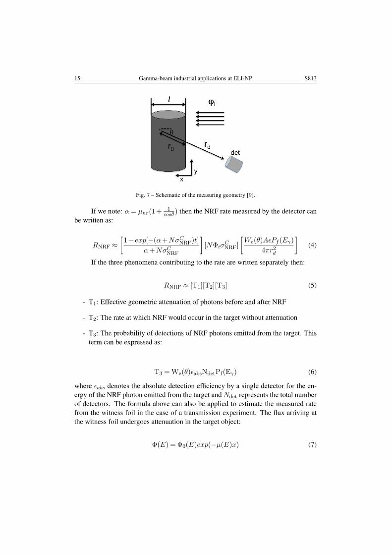
All the parameters that appear in the formula are defined for a slab of materialof thickness t as presented in Fig. 7.

Additional approximations are needed to simplify the formula:

- Neglect photon downscatter, so Φ(r) = Φ(x); Φ(E,x) = Φiexp(−µ(E)x)

- Neglect the energy dependence of photon absorption around resonance energy:µ(E) = µnr +NσNRF(E)

- Consider the resonance cross section as constant for the width of the resonance:σNRF(E) = σCNRF; E ∼ EC ; σCNRF =

∫σNRF(E)dE

ΓD



Fig. 7 – Schematic of the measuring geometry [9].

If we note: α= µnr(1 + 1cosθ ) then the NRF rate measured by the detector can

be written as:

RNRF ≈[

1−exp[−(α+NσCNRF)t]

α+NσCNRF

][NΦiσ

CNRF]

[We(θ)AεPf (Eγ)

4πr2d

](4)

If the three phenomena contributing to the rate are written separately then:

RNRF ≈ [T1][T2][T3] (5)

- T1: Effective geometric attenuation of photons before and after NRF

- T2: The rate at which NRF would occur in the target without attenuation

- T3: The probability of detections of NRF photons emitted from the target. Thisterm can be expressed as:

T3 = We(θ)εabsNdetPf(Eγ) (6)

where εabs denotes the absolute detection efficiency by a single detector for the en-ergy of the NRF photon emitted from the target and Ndet represents the total numberof detectors. The formula above can also be applied to estimate the measured ratefrom the witness foil in the case of a transmission experiment. The flux arriving atthe witness foil undergoes attenuation in the target object:

Φ(E) = Φ0(E)exp(−µ(E)x) (7)



which has two effects: the overall flux is decreased before the witness foil, and thenumber of photons in the resonance window is decreased proportionally with thenumber of resonant photons in the witness foil.

B. Transmission NRF experiment: comparison with similar experiment at HIγS

While the use of NRF for safeguards and nuclear waste management showsgreat promise, there are a few technical issues that need to be taken into accountwhen choosing the test case for the initial estimate of the feasibility. The first pointis that the information about the NRF resonances is not known for many nuclides ofinterest. Secondly, many of these materials have a special status in what concernsquantity and storage conditions, as well as in terms of manipulation. Also, it isdesirable to have an estimate for one of the cases that can be measured as soon aspossible after the commissioning of the experimental facility.

To address the most important issues, many of the experiments involving nu-clear sensitive materials are performed using surrogate materials. We will follow thesame course of action. The following numerical examples are given for the case ofdepleted Uranium (DU) used as surrogate for any of the actinides of interest and Wor Pb as surrogate for the matrix in which these actinides reside.

The first estimate of rates can be done for the experimental conditions describedin Ref. [5]. In this article, the photon beam delivered by HIγS is used in a transmis-sion experiment, where the role of the object is played by a 1.3 cm slab of DU,shielded at times by a slab of 1.3 cm of W. The role of the notch detector is playedby a thick DU target, followed by a Cu witness foil for beam normalization. Fourhigh-purity-germanium HPGe coaxial detectors (60% relative efficiency) were posi-tioned at backward angles relative to the beam and facing the witness foil location.Absorbers of 4 mm thick Cu and 4.5 mm of Pb were placed on the front face of eachdetector to reduce low energy background. Hagmann et al. [5] shows that the totalnumber of NRF event is 110 in the most unfavorable case after 25.5 hours of measure-ment and concludes that a 6 hours measurement would be required for a six-sigmalevel detection of sensitive material in the object when using the 100 photons/eV·sflux at HIγS.

The table below presents the expected NRF rate estimated for the experimentalconditions at ELI-NP. Each of the columns details the components of the analyticalrate of detection of the NRF formula that was used in the calculation for one scenario.The scenarios evaluated in the calculations are, in the order of the columns:

I. No object (thickness of UO2 and W shield set as 0). All incoming flux reachesthe notch detector

II. 1.3 cm thick W shield is placed downstream of the detector



III. 1.3 cm thick UO2 surrogate SNM material is placed downstream of the detector

IV. 1.3 cm thick W shield and 1.3 cm thick UO2 surrogate SNM material are placeddownstream of the detector, in a ’typical’ scenario of hidden SNM

The number of photons used in the calculations (Table 8) is the estimatednumber of photons coming from the source within the 1.78 eV Debye width ofthe resonance, and using a conservative value for the spectral density of 2.8×104

photons/s·eV.In conclusion, in the most unfavorable case, the same statistics as in the experi-

ment at HIγS can be reached in less than two minutes. The three orders of magnitudedifference can be roughly attributed to the two orders of magnitude difference in in-tensity and one order of magnitude from the detector array efficiency. It should benoted that the setup at ELI-NP considers that a 2 cm thick absorber is placed betweenthe detectors and the notch target, to attenuate the low energy Compton backgroundcoming from the scattering on the target of the other photons in the beam, as opposedto the 0.5 cm used at HIγS.

2.3.4. NRF applications – Isotope Imaging

A high penetrability and a weak element dependence of attenuation coefficientsof several MeV gamma-rays make possible to visualize density distribution inside amassive object by a technique of Computed Tomography (CT), which measures thetransmittance of gamma-rays through objects. The CT technique will be discussed indetail in section 3. Besides, a distribution of nuclei of interest inside an object is alsopossible to be visualized by measuring NRF gamma-rays as described in section 2.1.

In this section we propose to use the transmission NRF method to obtain CTimages of the isotope distribution inside objects. The attenuation of NRF events ab-sorbed in the measuring object can be inferred from the NRF events from a notchtarget placed downstream. To examine the feasibility of the CT imaging of the spe-cific isotope we made a simulation of the CT reconstruction of an isotopic (238U)distribution in an object that consists of some dense materials using GEANT4 simu-lations.

A. Simulation setup

A simulation was performed using the GEANT4 Monte-Carlo simulation code.Since the NRF interaction is not included in the original GEANT4 code, a modifiedversion of GEANT4, which takes into account all NRF processes, developed by ourgroup [10], was employed in this work.

A schematic drawing of the simulation setup is shown in Fig. 8 [26]. The LCSgamma-ray beam comes from the left side of the figure. The gamma rays irradiate



Table 8

Expected NRF rates for experimental conditions at ELI-NP

I II III IV NotesE(MeV) 2.1 2.1 2.1 2.1UO2(cm) 0 0 1.3 1.3 SNMW(cm) 0 1.3 0 1.3 shielding

m(g) DU 1.88 1.88 1.88 1.88 notchV(cm3) 0.10 0.10 0.10 0.10 notch

Beam spot diameter(cm) a 0.5 0.5 0.5 0.5t(cm) b 0.5 0.5 0.5 0.5

Φ0(phot/s/ΓD) 50000 50000 50000 50000 beamΦi(phot/s/ΓD) c 50000 16755 388 130

T1 0.19 0.19 0.19 0.19µnr(cm2/g) 0.05 0.05 0.05 0.05

α d 0.91 0.91 0.91 0.91σCNRF(cm−1) e 3.74 3.74 3.74 3.74

ΓD(eV) 1.78 1.78 1.78 1.78t(cm) 0.5 0.5 0.5 0.5

T2 186832 62607 1451 486Φi(phot/s/ΓD) 50000 16755 388 130

T3 0.1 0.1 0.1 0.1W(θ) 1 1 1 1Pf f 0.36 0.36 0.36 0.36ε(%) g 0.3 0.3 0.3 0.3Ndet 8 8 8 8

RNRF (counts/s) 311 104 2 1

aDiameter of notch detector is the same as that of the beambThickness calculated from the notch mass and beam diametercIncident flux of resonant photons on the notch target; The expected flux is extrapolated from the

values in the table in Ref. [2], supplied by constructordUsing a thin pin as a notch target, with detectors at 90.eThe integrated cross section for the 2.1 MeV resonance in 238U is 87 eV·b ([9])fDue to a 2 cm thick Pb absorber around the targetgConservative value. More details in the description of the setup section

the measuring object located on the beam axis. The object was rotated around ahorizontal axis and moved vertically to obtain projection images. Downstream of theinvestigated object, a 25 cm thick lead wall was installed to protect the gamma-raydetector from radiation scattered from the object. The wall had a through hole on thebeam axis for gamma rays, which were transmitted through the object. A notch targetwas located behind the wall. The notch target consists of pure 238U and its thicknesswas 5 mm. The attenuation of gamma-ray at NRF resonant energy was measuredby counting NRF gamma-rays from 238U in the notch target. The detection system



consists of 16 HPGe crystals installed at 90 degree and 16 HPGe crystals installed at135 degree. The diameter of the HPGe crystal was 6 cm and its length was 9 cm. Inthe actual ELI-NP spectrometer, each crystal will be segmented into 8 parts, but inthis simulation each crystal was treated as one detector.

Fig. 8 – A schematic drawing of the target and detectors layout. LCS gamma rays come from the leftside. A 25 cm lead wall protects the 32 HPGe detectors for NRF gamma-ray detection from radiationsscattered from the measuring object. The penetrability of gamma-rays at the resonant energy of 238Uwas measured by NRF gamma rays scattered on 238U target located downstream of the lead wall. Theattenuation of the whole gamma beam was measured by a LaBr3 detector installed on the beam axis.

Fig. 9 – A cross-sectional view of the measured object. The outer diameter of lead tube is 5 cm and itsthickness is 2.5 mm. Inside the tube, two 2 cm thick 235U and 238U rods are inserted and the tube is

filled with gallium.



A cross section of a measured object is shown in Fig. 9. The object consists of a5 cm outer and 4.5 cm inner diameter lead tube (density ρ = 11.34 g/cm3, attenuationcoefficient µ/ρ= 4.606×10−2 g/cm2) and 2 cm thick 235U and 238U rods (ρ = 18.95g/cm3, µ/ρ = 4.878× 10−2 g/cm2). Between the tube and these rods, gallium (ρ =5.904 g/cm3, µ/ρ = 4.113×10−2 g/cm2) was filled. In transmittance measurementof whole gamma-ray beam, the centroid energy of incident gamma-ray was 2176keV which is equal to NRF resonant energy of 238U and its energy spread was 0.5%in standard deviation which is the same as the ELI-NP specification. An incidentphoton number of 106 were considered for each measurement. This photon numberis equivalent for the number of photons in one macrobunch. An attenuation factorwas evaluated from a summation of energy deposit of all photon arrived at the LaBr3

detector.On the other hand, the fraction of gamma rays which energy is within a resonant

width is only 10−4. Thus, for attenuation measurement at NRF resonant energy,a monoenergetic gamma-ray beam was used to reduce the computation time. Theincident photon number was equivalent for 100 sec. In the simulation, transmittancewas measured at every 30 degrees (6 projection angles) by rotating the measuredobject and at every 1 mm (64 points) by scanning along the vertical direction. Anenergy distribution of gamma-rays detected by HPGe crystals is shown in Fig. 10.The two narrow peaks shown in the inserted frame are NRF peaks. The peak at higherenergy is gamma-ray emitted by a transition to the ground state and lower one is tothe first excited state (Ex = 44.9 keV). A broad peak at the foot of the higher energypeak is caused by elastic scattering on the notch target. The spectrum was obtainedusing a realistic ELI-NP gamma-ray beam energy profile and 2×109 incident photons[26]. The attenuation factor at NRF resonant energy was obtained from the yields ofthe narrow peaks. An example of the obtained projection image is shown in Fig. 11.

B. CT image reconstruction

CT image reconstruction was obtained using a filtered back projection methodfrom 6 (one dimensional) projection images. The filter employed was the Shepp-Logan filter. The reconstructed images are shown in Fig. 12. In the figures, thelarge attenuation part is expressed with white. The left panel of Fig. 12 shows thedensity distribution obtained by whole gamma-ray attenuation factor, i.e. a stan-dard CT image. The middle panel is reconstructed using the NRF yields. 238U rodis clearly enhanced compared with 235U rod. However, because of attenuation byother processes than NRF, other materials are visible also. These attenuations can beremoved by evaluating the whole energy spectrum. The figure on the right panel rep-resents the NRF yields normalized by the transmittance of whole energy gamma-ray.Consequently, we can clearly obtain an image of the 238U rod and conclude that the



Fig. 10 – A typical energy spectrum obtained by HPGe detectors calculated by GEANT4. Insertedpanel is an expansion around the NRF resonant energy. The two narrow peaks are gamma-rays from a

nuclear resonance on 238U.

Fig. 11 – An example of NRF projection image obtained by scanning the measured object. By rotatingthe object, 6 projection images are obtained. The grey disk indicates the 238U rod.

proposed method to visualize the isotope distribution could be feasible in the ELI-NPsetup.



Fig. 12 – Cross-sectional images obtained by whole beam attenuation factor (left panel) and by NRFgamma rays (middle). Right panel image is reconstructed by the ratio of NRF gamma strength to

transmittance of whole energy gamma beam. In the figures, the white parts are equivalent to stronggamma-ray attenuation sections.

2.4. TECHNICAL PROPOSAL

The NRF experimental setup will use the ELIADE array being developed forthe dedicated NRF experiments. Its full description, location, mechanical supportstructure, vacuum, cooling and other requirements are detailed in the respective TDR.For scattering experiments, the object of interest will be placed at the target positionof the ELIADE array. This can be used for small objects (distance between thedetector face and centre of the array is between 15 cm and 25 cm). For transmissionexperiments, the notch detector will be placed at the centre of the array, and the objectto be scanned on the tomography table, somewhere before the detector array.

3. RADIOSCOPY AND TOMOGRAPHY

3.1. INTRODUCTION

Radiography and tomography are imaging techniques that use ionizing radia-tion as an interrogation probe for medical or industrial purposes. Unlike radiography,which produces two-dimensional (2D) transmission images of 3D objects, computedtomography (CT) yields cross-sectional images that can be successively stacked up tocreate a 3D reconstruction of an object. Both methods are widely used in medical di-agnostics nowadays using mainly X-rays or low energy gamma sources. In industry,gamma-ray CT had been mostly used in industrial columns/reactors to determine thephase distribution, phase separations and other non-uniformities inside two- or three-phase flow units [27–29]; an overview of the previous literature on computed tomog-



raphy used for industrial applications is published in Ref. [29]. Contrary to medicalapplications, usage of radiography and CT in industrial applications had limited ap-plicability so far because industrial sized-objects require high-energy/high-intensitygamma beam for penetration [29].

With the new developments in the production of high-energy gamma beamsby LCS technique, the interest in using CT tomography for industrial purposes hadrecently increased [18, 30]. Today there are several laboratories in the world thatcan produce high-energy gamma beams by the LCS and only few of these that candeliver high intensities as well [30, 31]. The future gamma source at ELI-NP willdeliver both high-intensity and high-energy gamma beams being the perfect solutionfor industrial applications in tomography. The source beam intensity is with few or-ders of magnitude higher than any other gamma-ray source available increasing sub-stantially the penetration length and respectively the maximum size of investigatedobjects. The quasi-monochromatic and high-intensity source characteristics allowacquiring an energy-selected data from the entire scattered and attenuated beam. Forexample, only by considering the small-angle scattered γ rays, a significantly im-provement in image sharpness is obtained even for large-size and strongly scatteringobjects. In addition, the small beam width, allows achieving good resolution imagesfor in-depth large objects technologies investigation, like: bonding in aeronautics,welding and machining accuracy in automotive industry, large concrete parts in con-structions [30]. The γ-ray source with a tunable energy feature is very useful inadapting the energy range with the scanned object composition, for correctly reveal-ing in the image the combination of different-attenuation materials, like plastic orceramic with metals parts. Based on this feature, the dual/multi-energy techniquecould be also applied for scanning an object at different energies and obtaining infor-mation about its component materials like, for example, density and atomic effectivenumber.

Based on the unique characteristics of the gamma-beam at ELI-NP we proposea Digital Radioscopy and Tomography (DRT) setup that will allow the investiga-tion of industrial-sized object with high resolution and high contrast sensitivity. Thissetup will be specialized in non-destructive experiments and analysis by performing2D transmission images and 3D reconstructed tomographs of the scanned objects,revealing the internal fine structure and composition, very useful in the develop-ment of processes for new technologies and materials and also for industrial com-plex structures analysis. Moreover, this setup may also be employed in performingisotope-specific imaging/mapping through the use of nuclear resonance fluorescencetechnique.



3.2. METHODS

To perform radioscopy and tomography at ELI-NP we propose a first genera-tion tomography setup (pencil-beam) with a highly collimated beam. Toyokawa etal. [32] proved the working principle of a high-energy gamma-ray imaging systemfor industrial objects using a pencil-beam setup. They imaged several objects madeof either low Z (concrete) or high Z (Pb, Fe, Cu) materials or a combination of thetwo [30, 32, 33]. The best spatial resolution attained using 10 MeV LCS photons was650 µm, which was obtained using a 1 mm collimator placed after the object and alarge (8 in x 12 in) NaI detector. Similar results were obtained at HIγS facility, whereusing a CCD-based gamma camera detection, they demonstrated a lateral resolutionof 0.5 mm and a contrast sensitivity better than 6% [34]. At ELI-NP we expect toachieve a better spatial resolution and higher contrast sensitivity since the intensityof the ELI-NP gamma beam will be few orders of magnitude higher. More detailsabout the performance of such setup will be presented in the following section.

Figure 13 shows a schematic view of the proposed DRT setup. A small-openingcollimator placed after the object will define the beam width and the spatial resolutionof the setup. In practice, usage of highly collimated beams is a trade-off betweenresolution and detection efficiency, therefore the targeted resolution for this setup islimited to sub-millimeter range. Nevertheless, in certain conditions (small or mediumobjects made of low Z materials) one can aim for a better spatial resolution that canreach up to 100–200 µm.

Fig. 13 – Schematic view of the ”pencil-beam” setup.

3.3. FEASIBILITY OF THE PROPOSED METHODS IN ELI-NP CONTEXT

In tomography an object is scanned along several directions (named projec-tions) and an image of its cross section is obtained through image reconstruction. Acollection of such 2D images (”slices”) measured along the height of the object canbe used to construct a 3D view of the object. The performance of the DRT system de-pends on three parameters: spatial resolution, contrast and temporal resolution. Thespatial resolution and the contrast are crucial parameters in scanning large industrialobjects with high resolution, where as the temporal resolution is mainly important for



the investigation of dynamic processes. All three parameters are interrelated and af-fect the cost of the tomography setup so often a compromise is sought to achieve thebest performance. The spatial resolution of a tomography system depends stronglyon a few parameters, namely: the width of the beam, the number of projections andthe number of detectors/projections. The contrast, i.e. the lowest measurable den-sity difference, is greatly influenced by the intensity of the gamma beam and by theefficiency of detection. To study the feasibility of the proposed setup we rely onanalytical calculations and numerical simulation in GEANT4 [24, 25].

3.3.1. Analytical calculations

To assess the performance of the DRT setup we estimate the spatial resolu-tion and the contrast sensitivity using line-pair structures (line pairs per mm – LPM)[35]. In practice, we measure the contrast of a standard grid against the backgroundprovided by a homogenous object. Such a grid, made usually from stainless steel(SS) contains both linear and vertical bars. A diagram of such a grid is shown inFig. 14. The thickness and the width of the bars are equal, and also equal with thespacing between two consecutive bars. The fact that we also vary the thickness ofthe bars allows us to determine the contrast sensitivity, not only the spatial resolution[30, 35]. For our estimates, the grid parameter, a, is varied from 2 mm to 0.1 mmcorresponding to a resolution of 0.25 LPM to 5 LPM.

In the following, we present an analytical model for the pencil-beam tomog-raphy setup, which is used to estimate the resolution and the counting rates on thedetector as well as the optimal parameters to be used in the simulation.

Figure 14 illustrates a schematic drawing of the experimental setup. The pho-tons emitted from the interaction point pass through the ELI-NP collimator, lead-ing to a highly collimated beam within the specifications (106 photons/macrobunchwithin 0.5% energy FWHM (full width at half maximum), see Ref. [2]). The photonbeam then crosses the object, made in our calculations from a uniform object and aregular grid, and is then detected by a large size detector after passing through an-other collimator. The latter is used to define the beam width but also to reduce thescattered photons influence.

Depending on the size of the tomography collimator and of the distance be-tween the detector and interaction point, the total number of photons coming fromthe source that reach the detector when the object is missing is given by:

I = I0

(RCDθ

)2

(8)

where I0 is the source intensity, Rc is the radius of the tomography collimator, Dis the distance between the interaction point and the tomography collimator, and θ



is the angular opening of the source. In this calculation we assume that the maincollimator is fixed and outside the scope of this TDR. Same assumption is made forthe source. Another section will deal with improvements of the tomography setup,which can be attained by altering the beam properties and the ”standard” opening ofthis collimator.

Fig. 14 – Schematic drawing of the experimental setup and of the grid used to assess the resolution.

As a result, in the first approximation, the source is:

• Monoenergetic: 0.5% FWHM is very small on the scale of the variation of theabsorption coefficient

• Uniform: the density of photons within the solid angle is uniform

As we scan the beam across the grid, the number of photons reaching the detector willvary, increasing and decreasing as the beam intersects the grid or not. The number ofphotons reaching the detector when the beam passes between the grid bars is givenby:

NMAX = Ie−µxtε (9)

where I is the available source intensity computed in equation (8), t is the acquisitiontime, ε is the efficiency of the detector, µ is the attenuation coefficient in the uniformobject, and x is the object thickness.

The number of photons reaching the detector when the beam passes throughthe grid bar is given by:

NMIN = Ie−µGae−µxtε (10)



where µG and a are the absorption coefficient of the grid and thickness of the grid.If we assume that the spot size of the beam reaching the detector at the grid positionis smaller than the dimension of the grid bar then the beam reaching the detector willbe modulated by the grid thickness. This can be written as:

RCD

=fa

d(11)

where f is a measure of how smaller the beam spot is compared to a. A small f willimply a finer scan but also a smaller diameter of the collimator, which will reducegreatly the intensity of the beam. If the beam spot at the grid is smaller or equalwith a (i.e. a > 2θd) then the signal at the detector will be modulated by the grid,therefore no need for collimation.

Fig. 15 – A drawing of generic signal.

In order to decide if the grid is visible or not in the scan data we need to comparethe variation between NMAX and NMIN (Fig. 15). In practice, because of the smallthickness of the grid we only expect few percent differences between NMAX andNMIN, so a serious issue is whether the differences are significant from the point ofview of the counting statistics. To obtain good counting statistics in the detector weintroduce the following conditions:

A.

NMAX−NMIN > S√NMAX (12)

where S is a significance factor.

For S=2, the error bars of the two extreme points touch, so a higher contrast isgiven by a higher value of S.



We can write the equation for the time needed to attain a certain contrast S fora set of experimental conditions:

t=S2

e−µx

(d

fa

)2 θ2

I0ε

1

(1−e−µGa)2(13)

B. Alternatively we can use: NMAX−NMIN > S(√NMAX +

√NMIN)

which leads to:

t >S2

e−µx

(d

fa

)2 θ2

I0ε

1

(1−√e−µGa)2

(14)

Based on the analytical model the main conclusions are: the object has to be asclose to the source as possible and the measurement time scales with squared contrastS2 and with 1

a4for small a.

Numerical examples: Pencil-beam setup. To estimate the counting rates on thedetector and assess the optimal resolutions and contrast sensitivity that we can achievewith the ELI-NP tomography setup we apply the analytical model for two experimen-tal cases. For our estimates, the grid parameter, a, is varied from 2 mm to 0.1 mmcorresponding to a resolution of 0.25 LPM to 5 LPM. The grid parameter a equalsthe width and the thickness of the grid bars as well as the separation between the bars.Therefore, the values cited in the following numerical examples represent not onlythe spatial resolution but also the contrast sensitivity attainable for a SS material.

Case 1. The setup is located after the low energy interaction point in experimentalarea E2. The attainable energies at this location are 3.5 MeV or lower, however theestimations are extended to higher energies as well for cases when the setup willoperate at higher energies. For this numerical example we consider: D = 40 m,d = 20 m, t = 1 s, ε = 1, S = 10, f = 1/2 (the ”useful” diameter of the beam spoton the object is equal to a) and a stainless steel grid.

For the present case and according to equation (11) the collimator radius canbe expressed as: RC = faD

d = a.Table 9 lists the thickness for several materials for which we can achieve a

resolution of 0.7 mm (RC = 0.7 mm) in the tomography using the parameters de-fined above and using equation (12) for the counting statistics. The rates/macrobunch(number of photons within the bandwidth per macrobunch) in the detector are listedin the table and are in the order of 103 photons. The maximum thickness of the in-vestigated materials increases as we increase the energy of the gamma beam mostlybecause of the improved parameters of the gamma beam at high energy.



Table 9

Expected thicknesses for the case when the setup is after the low energy interaction point (case 1). The

first three rows list the gamma source parameters as received from the manufacturer and used in the

estimations (Ref. [2]).

Energy (MeV) 2 3.5 9.87 19.5Source divergence (µrad) 140 100 50 40Nr of photons withinFWHM bandwidth

4.0×108 3.7×108 8.3×108 8.1×108

Al (cm) 30 41.2 88.9 104.9Fe (cm) 10.4 13.5 23.7 24.3H2O (cm) 70.8 100.5 250.1 337.05Concrete (cm) 33.8 47 106.8 131.6Rates/macrobunch 1.9×103 2.9×103 3.9×103 3.4×103

Using the same analytical model we can estimate what is the highest resolutionthat we can achieve for certain materials and thicknesses if we limit the exposure timeto 1 second. As one can see in the Table 10 one can obtain sub-mm resolution forall low Z materials listed up to 50 cm thick. For higher Z materials like Fe, sub-mmresolutions can be obtained only for small to medium size objects.

Table 10

Estimated resolutions achievable for different materials and thicknesses at beam energy of 3.5 MeV.

Beam spot diameter is 4 mm at the sample and 8 mm at the collimator. The collimator has the inner

radius equal to the resolution that we seek. Number of photons/s is 3.7×108 and the source divergence

is 100 µrad.

Materials 10 cm 20 cm 30 cm 50 cmAl 0.35 mm 0.44 mm 0.55 mm 0.85 mmFe 0.55 mm 1.09 mm 2.15 mm 4 mm in 20 s a

H2O 0.31 mm 0.34 mm 0.37 mm 0.44 mmConcrete 0.34 mm 0.41 mm 0.50 mm 0.74 mm

aThe uncollimated beam spot is 4 mm at the object and this resolution can not be achieved in 1 sexposure time, only in 20 s

The values estimated in the tables are for large source-object distance (20 m),which represents one of the possible locations of the tomography setup in the experi-mental hall. Other possibilities for smaller object-distance exist as well and they willbe listed in the ”location of the experimental setup” section. Smaller source-objectdistances are advantageous when higher resolutions are sought. Estimates for such acase are displayed below.



Case 2. For this numerical example we consider D = 10 m, d= 5 m, t= 1 s, ε= 1,S = 10, f = 1/2 (the ”useful” diameter of the beam spot on the object is equal to a)and a SS grid.

As has already been concluded from equation (13) and (14) we can improve theperformance of the tomography setup by placing the object as close to the source aspossible. In this configuration we can either reduce the measurement time for scan-ning similar objects as in the previous case or scan significantly larger objects. Table11 lists the expected thickness of several materials for which we can achieve 0.7 mmresolution (RC = 0.7 mm) at reduced source-object distance. The rates/macrobunchin the detector are in the order of 103 photons/macrobunch. Note that in the esti-mations for 9.87 MeV and for 19.5 MeV, the beam does not need any collimation(except to remove scattered radiation) since the beam spot at the object is 0.5 mmand 0.4 mm, respectively. At these two energies the estimated numbers are for aresolution of 0.5 and 0.4 mm, respectively.

Table 11

Expected thicknesses that can be scanned when the object is closer to the source (case 2). The rates

per macrobunch are listed as well. The first three rows list the gamma source parameters as received

from the manufacturer and used in the estimations (Ref. [2])

.


4.0×108 3.7×108 8.3×108 8.1×108

Al (cm) 53.7 72.4 111.8 114.1Fe (cm) 18.7 23.8 29.8 26.5H2O (cm) 126.9 176.4 314.3 366.8Concrete (cm) 60.7 82.7 134.3 143.3Rates/macrobunch 1.9×103 2.9×103 3.9×103 3.4×103

Table 12 lists the calculated optimal resolutions that can be achieved for dif-ferent objects at high energies. The resolution depends on the collimator’s innerradius according to equation (11). Therefore these resolutions are achievable usinga collimator with an opening in radius equal to the resolution. As expected and alsoinferred from the tables, a smaller object-source distance will enhance considerablythe resolution. Table 12 presents the estimated resolutions when using high-energyphotons in case 2 example.

So far our estimates were done for exposures that last one second. The nexttables (Table 13 and Table 14) lists the estimated measurement times (in seconds)



Table 12

Estimated sub-millimeter resolutions achievable for different materials and thicknesses at beam energy

of 19.5 MeV in the case 2 setup. Beam spot diameter is 0.4 mm at the sample and 0.8 mm at the

collimator. Number of photons/sec is 8.1× 108 and the source divergence is 40 µrad.

Materials 10 cm 20 cm 30 cm 50 cmAl 0.09 mm 0.10 mm 0.12 mm 0.16 mmFe 0.15 mm 0.27 mm 0.4 mm in 2.44 s a 0.4 mm in 380 s b

H2O 0.080 mm 0.083 mm 0.087 mm 0.1 mmConcrete 0.085 mm 0.095 mm 0.11 mm 0.13 mm

aThe uncollimated beam spot is 0.4 mm at the object and this resolution can not be achieved in 1 sexposure time.

bsame as note a

for one exposure when scanning 10 cm of material with two different resolutions:0.2 mm (0.5% contrast) and 0.5 mm (1.23% contrast) using of 3.7×108 photons/sof 3.5 MeV energy. As expected the measurement times increase greatly for higherresolutions. Nevertheless, in case of a target resolution of 0.5 mm, the duration ofone exposure is comparable with the macrobunch duration, i.e. 10 ms, for most ofthe low Z materials of 10 cm thickness (see Table 13).

Table 13

Estimated measurement times (in seconds) for one exposure when scanning an object of 10 cm with

0.2 mm resolution (0.5% contrast for SS at 3.5 MeV). The source-object (collimator) distance is 5 m

(10 m).


4.0×108 3.7×108 8.3×108 8.1×108

Al 0.90 0.575 0.066 0.036Fe 7.97 3.54 0.369 0.250H2O 0.457 0.341 0.044 0.021Concrete 0.784 0.515 0.059 0.032

These times are calculated for a geometry in which the source-object (d) sourceis 5 m and the ratioD/d = 2. Usage of otherD/d ratio (magnification), can be scaledwith the opening of the collimator (equation 11), hence no change in the measure-ment time, however at increased source-object distances, the measurement times forone exposure will increase accordingly (see equation (13)). These values are esti-mated using a single large detector with efficiency 1. In practice the efficiency of the



Table 14

Estimated measurement times (in seconds) for one exposure when scanning an object of 10 cm with

0.5 mm resolution (1.23% contrast for SS at 3.5 MeV). The source-object (collimator) distance is 5 m

(10 m)


4.0×108 3.7×108 8.3×108 8.1×108

Al 0.023 0.015 1.7×10−3 9.3×10−4

Fe 0.206 0.091 9.5×10−3 6.4×10−3

H2O 0.012 8.8×10−3 1.1×10−3 6.2×10−4

Concrete 0.020 0.013 1.5×10−3 8.3×10−4

detector is lower and the measurement times will vary with 1/ε.

Improvements of the tomography setup: Cone-beam setup. If the single detec-tor is replaced by a 2D-array of detectors of small pixel size the total measurementtime will be scaled with the total number of detectors, hence faster times and higherresolutions can be achieved in certain conditions. For such configurations, the gammabeam must have a larger divergence (cone-beam) with a beam spot at least equal tothe area of the 2D detector. Such dedicated experimental setups are referred to as thefan-beam (linear array of detectors) or the cone-beam (2D-array of detectors) CT. Inthese cases, the targeted resolutions can reach 200 µm or better.

In the following we assess the feasibility of a cone-beam setup at ELI-NP. Themain assumptions are:

- Increasing the opening of the main collimator leads to a greater divergence ofthe gamma beam and increase photon flux and bandwidth (for example, frompreliminary data from EuroGammaS: 7×109 photons/s for a 1mrad divergence)

- Detection is performed using a detector array, like a flat-panel detector, or aCCD camera device [34, 36].

In general, a flat panel detector consists of a high number of pixels with eachpixel made of a small scintillator with limited thickness. So far on the market thesepixels reach up to 1 mm in thickness for columnar CsI(Tl) scintillator plates [37, 38].An important aspect when using flat-panel detectors for high-energy photons is theprobability of interaction of photons in the scintillators, which in this case is lotsmaller than 1.



The probability of interaction of photons in a scintillator (through all effects) isdefined by:

p= 1−exp(−Σx) (15)where x is the thickness of the pixel and Σ = n1σ1 +n2σ2 . The parameters: niand σi represent the number of atoms of the i-component in the scintillator per unitvolume and the total cross section, respectively. For instance at 3.5 MeV photons theprobability of interaction in a pixel of 500 µm for several scintillators is listed belowand as expected is larger for higher density scintillators.

Table 15

Probability of interaction of photons of 3.5 MeV in a pixel of 500 µm thick.

Scintillator material Density (g/cm3) pBGO 7.13 0.0138

CsI(Tl) 4.51 0.0082LSO 7.4 0.0139

In order to compare the two methods, pencil-beam and cone-beam CT, we com-pute the time needed to acquire a full scan of a small object by both methods. Tocalculate the total time we need first to define the total number of projections, namedhere P . The total number of projections has to fulfill the Nyquist-Shannon theorem:

P ≥ π

2S (16)

where S represents the number of sampling points in each projection line. S =φ/∆x, for an object of diameter φ and for a sampling step ∆x. Therefore the numberof measurements needed to scan a 2D slice of an object, i.e to acquire a 2D cross-sectional image, is

M = P ·S =π

2

φ2

∆x2(17)

If h∆z represents the total number of slices for an object of height h that is

scanned with a z-axis-sampling step ∆z, then we can define the total number ofmeasurements needed to obtain a 3D reconstruction of an object as:

N =π

2

φ2

∆x2

h

∆z(18)

Then one can estimate the total measurement time required for the completescan of an object as:

t= t1N for a pencil-beam setup



t= t2N

Npixelsfor a cone-beam setup

where t1 (t2) is the time for a single exposure in the pencil-beam (cone-beam)and Npixels represents the total number of pixels in the 2D-detector. For the cone-beam, the ”single exposure time” expresses the estimated measurement time for asingle pixel, i.e. considering only the fraction of the beam that falls on one pixel ofthe detector.

Next, we calculate and compare the time required to scan a small object throughboth methods: the pencil-beam and the cone-beam CT. The main assumptions are:

• Object: Aluminum (Al) cylinder of φ = 5 cm diameter and h =5 cm long (∼0.26Kg)

• Magnification D/d=2 (d=20 m)

• Cone-beam CT: source divergence is 1 mrad (beam diameter at object positionis 40 mm and 80 mm at detector position); the 2D detector is as large as thebeam spot and the pixel width is twice the resolution sought (2a)

• Pencil-beam CT: source divergence is 100 µrad (beam diameter at object po-sition is 4 mm, and 8 mm at detector position); the detector is a large volumesingle detector, e.g. 30 cm of NaI. The pencil beam is obtained with a collimatorthat has an opening equal with twice the resolution sought (2a)

• Eγ = 3.5 MeV

Table 16 lists the estimates for the measurement times for single exposures, formeasuring a single 2D slice with pencil-beam and the total time needed to scan asmall object (5 cm × 5 cm) in cone-beam and pencil-beam CT. In addition the tablealso lists the number of photons per macrobunch that are ”detected” in each case,considering a probability of interaction of 1 for the large volume detector (pencil-beam CT) and a probability of interaction of 1.6×10−2 for a 1 mm-thick pixel ofCsI (cone-beam CT). It is noteworthy to mention that as long as the number of pixelsin the detector is greater than the inverse of the interaction probability in the pixel,the cone-beam method is advantageous. Therefore the cone-beam method is usefulwhen scanning objects with great detail (high resolution and high contrast sensitiv-ity). However for cases when single 2D scans are required, the pencil beam is stilladvantageous. Note that this comparison between pencil-beam and cone-beam iscarried out at low energies (3.5 MeV) where the source divergence is larger than athigher energies. In the latter case the smaller beam spots and the larger number ofphotons per second constitute advantages for the pencil-beam CT.

To summarize, the analytical calculations allow us to estimate the thickness ofthe materials that can be investigated in the DRT system at certain targeted resolu-



Table 16

Comparison between pencil-beam and cone-beam CT when scanning a small Al object (5 cm × 5 cm)

with various resolutions at 3.5 MeV. CB=cone-beam; PB=pencil-beam; The probability of interaction

in 1 mm-thick pixel of CsI is 1.6×10−2

a (mm) Pixelthick-ness(cm)

Nr. ofmeasure-ments(N)

Nr. ofpixels(pixelwidth)

Nr. ofpho-tons/sec

Singleexpo-suretime (s)a

Timefor a2Dslicescan b

Total timefor a 3Dscan

Ndetected/mac-robunch

1 (CB) 0.1 1.96×105 1.26×103

(2mm)7×109 3.12 s 498 s 4.5×102

1 (PB) 30 1.96×105 1 3.7×108 0.01 s 39.2 s 1.96×103s 1.48×105

0.7(CB)

0.1 5.74×105 2.56×103

(1.4 mm)7×109 12.9 s 2952 s 2.2×102

0.7(PB)

40 5.74×105 1 3.7×108 4×10−2

s323 s 6.4 h 7.26×104

0.5(CB)

0.1 1.57×106 5.03×103

(1mm)7×109 49.3 s 4.36 h 1.1×102

0.5(PB)

30 1.57×106 1 3.7×108 0.15 s 2376 s 66 h 3.7×104

0.2(CB)

0.1 2.47×107 3.14×104

(0.4 mm)7×109 1.9×103

s417 h 1.8×101

0.2(PB)

30 2.47×107 1 3.7×108 5.9 s 164 h 4.1×104h 5.9×103

aFor the cone-beam, the ”single exposure time” expresses the estimated measurement time for asingle pixel, i.e. considering only the fraction of the beam that falls on one pixel of the detector. Thetime for a single exposure is estimated using condition (12) for S=10 to assure that we have enoughstatistics in each pixel of the 2D detector.

bThe measurement time needed to scan a 2D slice of the object is computed for the pencil-beamonly.

tions and calculate the expected detection times in order to have statistically signif-icant measurements. There is a significant increase in the measurable thickness orresolution if higher energies are used due to the improved parameters of the gammabeam at these energies. When seeking higher resolutions a cone-beam may be advan-tageous under certain conditions mentioned above. As expected, large objects can bescanned with higher resolution at smaller source-object distances.

3.3.2. Numerical simulations

As was already mentioned in the previous section the analytical calculationsare very useful in estimating detection rates and material’s thicknesses that can beinvestigated. Nevertheless, to assess the feasibility of our proposed DRT setup wealso rely on numerical simulations. The simulations are carried out in GEANT4[24, 25] where we have implemented all the components of the experimental setup.The modeled gamma source has a size between 10–30 µm and a divergence between



25–200 µrad depending on the energy of the beam [2].To test the spatial resolution and the contrast sensitivity of the tomography

setup we simulate the transmission through various objects and grids using GEANT4.To estimate the optimal parameters to be used in the simulation we rely on analyticalcalculations. In practice, we measure the contrast of a standard stainless steel gridagainst the background provided by a homogenous object as pictured in Fig. 14The scanning is done by moving the object and the grid by a fraction of a, wherea represents the width and the thickness of the grid. The results of the simulationconsist in either single line scans taken across the grid or in 2D-radiograph of thegrid.

The spatial resolution and the contrast sensitivity of the tomography setup werefirstly tested using water-based objects at low energies of the gamma beam. Thewater-based objects were used to mimic the attenuation in organic tissues. An ex-ample of a simulated 2D-radiograph of 5 mm grid is shown in Fig. 16. Because ofthe high number of exposures needed to simulate a 2D image of the entire grid weuse a relatively low number of photons in the source (1×106) and a thick grid. Forvery thin grids (weak contrast) one needs a good counting statistics in the detectorshence a high number of photons in the source. In order to reduce the computationaltime we limit the number of the exposures by investigating the gamma transmissionthrough the grid+object for single-line scans taken across the grid rather than 2Dradiographs. Figure 16 illustrates single-line scans across a stainless steel grid of dif-ferent widths/thicknesses. The grey boxes show the location of the grid bars. As onecan clearly see, the grid is distinguishable even for 0.25 mm width/thickness. Thishigh resolution is possible due to the small opening of the tomography collimatorused, which is 0.2 mm in diameter and thanks to the low attenuation in the object.

In the pencil-beam configuration, the degree of collimation of the beam definesthe spatial resolution of the setup. Highly collimated beam imply lower beam inten-sities, hence a compromise must be reached between spatial resolution and detectionefficiency. Figure 17 presents the simulated grid profile of 0.38 mm grid placed infront of an Al object for different opening of the collimator (RC) located at 10 mfrom the source (D/d = 2). Thickness of the Al object is varied to obtain similarcounting statistics in the detector (Table 17). The simulation results indicate that inorder to maximize the counting statistics for a given resolution, the size of the col-limated beam (see equation (11)) can be as large as aD/d , i.e. f = 1/2 . In ourparticular case studied here, the collimated beam diameter is twice the resolutionsought (D/d= 2).

To validate our simulations we compare them with analytical curves. Figure18 presents the results of the tomography simulations for an Al object of 10 cmthickness. This object was scanned with 2.3×107 photons at energy of 3.5 MeV ±17 keV in a geometry similar to that described by case 1 in section 3.3.2. (source-



5 mm

0 5 10 15 20 25 30

scan step a/2

0

5

10

15

20

25

scan s

tep a

/3

1000

1100

1200

1300

1400

1500

1600

Fig. 16 – Number of 2 MeV photons that reach the face of a detector after passing through a 10 cmwater-based object and a grid of variable thickness/width. The left panel presents a 2D-radiograph fora= 5 mm grid and the right panel shows single-line scans for several grid dimensions. The source had

1×106 photons in the left panel and 1×108 photons in the right panel. The color scale reflects thenumber of photons that reach the detector. The source-object distance is 5 m, the magnification is 2.

object distance of 20 m with magnification 2). The transmitted beam was collimatedusing a collimator with an inner radius of 0.7 mm, an outer radius of 10 cm and 20 cmlong. A good agreement between the analytical model and the simulation is obtainedwith a systematic difference of 3% in the intensity at the detector.



Fig. 17 – Number of photons that reach the detector after passing through an Al object and a 0.38 mmSS grid for different collimated beams at Eγ=3.5 MeV. The grey boxes show the location of the grid

bars.

Table 17

Maximum thickness measurable with a resolution of 0.38 mm (1% contrast) at 3.5 MeV for differentcollimated beams. The source used has 1×108 photons. The source-object (-collimator) distance is5 m (10 m). Assuming a beam divergence of 100 µm, the diameter of the beam spot at the sample is

1 mm and 2 mm at the detector. Through further collimation the beam spot at the sample can be

reduced according to equation (11).

f RC (mm) Al(cm) Concrete (cm) Fe (cm)0.137 0.1 1.2 1.4 0.40.25 0.19 14.74 16.82 4.840.5 0.38 30.33 34.61 9.971 0.76 45.92 52.41 15.09

3.4. CT RECONSTRUCTIONS

An important and crucial part of the computed tomography is the image recon-struction process. Using mathematical algorithms a 3D image of an object can bereconstructed from its projections.



Fig. 18 – Comparison between the Monte Carlo simulated and the calculated number of transmittedphotons using the analytical model. The object is an Al cylinder of 10 cm thickness in the beam. Thegray boxes show the location of the grid bars. The grid bars are 0.7 mm in width and thickness. Theanalytical curve was vertically displaced upwards (corrected with the 3% difference) to overlap the

simulation data. The error bars represent the squared root of the number of events.

Figure 19 presents the reconstructed CT images of simulated data. The objectis a cylinder of 45 mm diameter with walls of 2.5 mm thick that is made of a materialthat has the linear attenuation coefficient 0.5 cm−1. The cylinder is filled with aliquid having µ = 0.2 cm−1 and contains a heavy metal (µ= 0.9 cm−1) rod inside.For the simulations we use 500 detectors placed in a linear array. The high number ofdetectors implies a resolution as low as 90 µm. The number of projections needed toreconstruct a 2D-cross-sectional image of this object is 785 according to the Nyquist-Shannon theorem. Figure 19 shows the simulated CT reconstructions as a function ofthe number of projections. Note that a good quality image can also be obtained withhalf the estimated number of projections. The CT reconstruction is done using thefiltered-back projection algorithm together with a Sheep-Logan filter. We calculatedthe signal to noise ratio for each tomography to emphasize the higher quality of theimage when using larger number of projections.

Measurement time estimations for obtaining a 2D cross-sectional image con-sidering the expected ELI-NP gamma-beam capabilities are listed in Table 16 for a



similar size object, using pencil-beam CT. Note that depending on the complexity ofthe object good quality images can be obtained with smaller number of projections.

50 projections 100 projections 200 projectionsS/N = 0.25 S/N = 0.41 S/N = 0.84



Fig. 19 – CT reconstructed images of simulated data. The number of projections used and the signal tonoise ratio (S/N) are specified below each image.



3.5. TECHNICAL PROPOSAL

Figure 20 illustrates a diagram of the pencil-beam DRT setup proposed at ELI-NP. The main components are labeled in the figure and their detailed descriptionwill follow. The picture depicts a particular geometry for the case of large-objectinvestigations however there is flexibility in adjusting the geometrical parametersfor smaller sample investigations. The geometrical and spatial parameters will bepresented in the section dedicated to the location of the experimental setup. Figure21 illustrates the diagram of the 2D-high energy gamma detector that can be used forcone-beam tomography.

Fig. 20 – Digital radiography and tomography pencil-beam gamma-ray setup for large-size samplesfor industrial applications.

3.5.1. Location of the experimental setup

So far in the estimations we have used two examples for the setup geometries,one at low energies and one at high energies. In practice, at low energies we haveup to 60 m for placing the object and the detector. This 60 m is roughly the lengthof the 2nd part of the accelerator, leading to the second interaction point. Whilewe also show the numbers for the high-energy gamma beam, we worked under theassumption that the tomography setup will first be placed at the low-energy pointso that we can start measuring from the start of the machine operation. Once thehigh-energy beam will be available, we can move equipment there based on spacelimitation.



Fig. 21 – Schematic diagram of the high-energy 2D gamma detector for cone-beam CT.

3.5.2. Sample positioning system

The sample positioning system will consist of two tomography tables (one largeand one small) to be used in different locations of the laboratory to be in agreementwith the space and the weight limit. One table will be dedicated to large and heavyobjects while another will be dedicated to small and light objects. The characteristicsof the two tables are listed below.

• X- (Y-) axis travel: 1500/150 mm

• Z-axis travel: 2000/250 mm

• Max load: 150/10 Kg

• Positioning resolution: 10 µm, 0.05 (30 µm, 0.1 )

• Speed: between 0.1 mm/s and 5 cm/s, with programmed ramps, speed accuracy:0.5%

In addition to the tables, the setup needs the following components:

• Position sensors for all axes

• Feedback DSP based real-time positioning and speed control.

3.5.3. Collimators

The feasibility study indicated that a high degree of flexibility is needed inchoosing the opening of the collimator in order to maintain a high speed for scanningobjects as well as a good counting rate in scanning large objects. Therefore to gainsuch versatility a variable opening collimator from 0.1 mm to 3 mm will be optimal.



However due to the complexity of such collimator and its high price at the beginningwe will use sets of individual collimators. The collimators will be made of lead (Pb)or tungsten (W) with various collimation holes: 100 µm, 200 µm, 500 µm, 700 µm,1 mm, 3 mm, 6 mm. The collimators will need mechanical supports and alignmenttables equipped with X, Y and Z scale-movement and rotation.

3.5.4. Detectors for the DRT setup

Fig. 22 – Time structure of the gamma beam. A macrobunch consists of 32 micropulses, which repeatevery 16 ns. The repetition rate for macrobunches is 100 Hz.

The rates per macrobunch in the detector for a tomography experiment were es-timated to be between 100 and 10000 photons/macrobunch depending on the gamma-beam energy, the object thickness and the source-detector distances. Such high ratesof high-energy photons represent an outstanding challenge for detection complicatedeven more by the peculiar time structure of the beam (Fig. 22). At high photonsenergies, detectors based on scintillator crystals are more practical than any otherdetectors because of their high efficiency. The characteristics of some common scin-tillators are present in Table 18. The ideal choice of a detector for the pencil-beamsetup would be a scintillator with high stopping efficiency; however a large NaI(Tl)(8 in × 12 in) would fulfill same requirement and could represent a good choice tostart with as is often used in tomography setups. Another choice may be a LaBr3

scintillator for cases when the transmitted gamma beam is too intense and wouldcause significant pile-up in the detector. Since the LaBr3 has the shortest decay time(comparable with the microbunch time interval) it may help avoid or at least reducethe pile-up events. In case of the cone-beam measurements, a flat-panel detector,or a CCD camera-based device can be considered. A CCD-based imaging deviceconsists of a scintillator plate that converts the incident radiation into visible photonsand a CCD camera that detects them [34]. The advantage of using a CCD camera-based device over the single radiation detector stands in its relatively small pixel size(down to tens of micrometers). In addition, for high-energy photons we may considera CdTe flat-panel detector. For the isotopic measurements that combine CT tomog-raphy with NRF based detection, we will use the transmission NRF method and itsdetector system described in section 2.

To overcome the issue of high number of photons/macrobunch we will use a



Table 18

Scintillator characteristics

Detector NaI(Tl) CsI(Tl) BGO LSO LaBr3

Density (g/cm3) 3.67 4.51 7.13 7.35 5.29Lrad (cm) 2.59 1.85 1.12 0.88 2.1

Decay time (ns) 230 1000 300 40 16Light yield (photons/keV) 38 54 8-10 25 63

Luminescence (nm) 410 530 480 420 380Hygroscopic Yes Slightly No No Yes

photomultiplier (PMT) with adjustable gain over a large range (few orders of magni-tude). For example R1250 PMT from Hamamatsu has a voltage adjustable gain thatspans over 6 orders of magnitude.

3.5.5. Electronics and DAQ

Figure 23 presents a schematic of the electronics and interconnections requiredfor operating a DRT setup. The three main components of the diagram are: thesample positioning system, the movement control system and the data acquisitionsystems.

Fig. 23 – Schematic of the electronics and interconnections.



3.5.6. The mechanical support structure

The mechanical support structure for the translation tables will consist of astack of three one-directional tables. Because they are general-purpose objects, theirdetailed design depends on the precise implementation by the producer and hence isdependent on results of the tender procedure. ELI-NP will only design the couplingbetween the tables and ensure their proper placement inside the experimental hall.

The support structure for the detectors and collimators is a simple one, with thedetectors and collimators being aligned with the beamline using the global networkof reference points.

3.5.7. HV and LV power supplies

The voltage requirements of the setups require general 220 V, 50 Hz powerconnectors. The HV for the scintillator detectors will be supplied by NIM modulesinside a crate. The power supplies for the low-load table will be most likely of lowvoltage DC (24 V - subject to manufacturer specifications) while for the high-loadtable will be probably 220 V AC (subject to the manufacturer specifications).

3.5.8. Cabling

The DRT setup will use cables of various types and length to interconnect:

• The small and big table components with PC and Movement Controllers

• PC with Movements Controller, Detectors and Gamma Beam Control Room

• The setups in the experimental hall with the general data stream and controls ofELI-NP.

4. SPECIFIC NEEDS AND UTILITIES, TRANSVERSAL NEEDS

The implementation of this TDR will rely on the available ELI-NP infrastruc-ture: electronic and mechanical workshop; clean room for detector assembly andstorage; high speed 10Gb/s Ethernet or Infini band data connections from experi-ment to control/data acquisition room; high speed data storage system; radioactivesources for detector testing and calibration; clean power supply lines; clean ground-ing connections.

5. COLLABORATIONS

A memorandum of scientific collaboration exists with: The Institute of Ad-vanced Energy, Kyoto University, Japan and ACCENT PRO 2000 s.r.l. Bucharest,



Romania.

Acknowledgements. The ELI-NP project is co-funded by the European Union through theEuropean Regional Development Fund. The authors would like to acknowledge the help received fromthe engineering bureau, especially from Cristian Petcu and Emil Udup.

REFERENCES

1. Extreme Light Infrastructure-Nuclear Physics White Book,url: http://eli-np.ro/documents/ELI-NP-WhiteBook.pdf

2. O. Adriani et al., Technical Design Report EuroGammaS proposal for the ELI-NP Gamma beamSystem, arXiv:1407.3669 (2014).

3. W. Bertozzi and R. J. Ledoux, Nucl. Instr. and Meth. Phys. Res. B 241, 820 (2005).4. G. Warren, J. Caggiano, and P. Peplowski, AIP Conference Proceedings 1194, 106 (2009).5. C. A. Hagmann et al., J. of Appl. Phys. 106, 084901 (2009).6. D. L. Chichester, Industrial applications of photonuclear resonance excitations, Thesis 2000, url:

http://dspace.mit.edu/handle/1721.1/292987. R. Hajima, T. Hayakawa, N. Kikuzawa and E. Minehara, J. Nucl. Sci. Tech. 45, 441 (2008).8. J. Pruet, D. P. McNabb, C.A. Hagmann, F.V. Hartemann, and C. P. J. Barty, J. Appl. Phys. 99,

123102 (2006).9. B.A. Ludewigt, B. J. Quiter, and S.D. Ambers, Nuclear resonance fluorescence for safeguards

applications, DOE report, url: http://dx.doi.org/10.2172/1022713 (2011).10. H. H. Negm, Studies on the optimum geometry for a nuclear resonance fluorescence detection

system for nuclear safety applications, Thesis, Kyoto University (2014).11. N. Kikuzawa et al., Appl. Phys. Express 2, 036502(2009).12. T. Hayakawa et al., Rev. Sci. Instr. 80, 045110 (2009).13. B. J. Quiter, Nuclear resonance fluorescence for nuclear materials assay, Thesis, url:

https://escholarship.org/uc/item/0kc2s2kn, Univ. California, Berkley(2010).

14. B. J. Quiter, B. A. Ludewigt, V. V. Mozin, and S. G. Prussin, IEEE Trans. on Nucl. Sci. 58, 400(2011).

15. O. Beck et. al., J. Appl. Phys. 83, 5484 (1998).16. CODEX General Standard for Contaminants and toxins in food and feed, Codex Standard 193-

1995 (1995).17. M. N. Lakshmanan, B. P. Harrawood, G. A. Agasthya, A. J. Kapadia, IEEE Trans. On Med. Imag.

33, 546 (2014).18. H. Toyokawa et al., Jap. J. of App. Phys. 50, 100209 (2011).19. D. Vartsky, K. J. Ellis, D. M. Hull and S. H. Cohn, Phys. Med. Biol, 24, 689 (1979).20. L. Wielopolski, R. C. Ancona, R. T. Mossey, A. N. Vaswani, and S. H. Cohn, Med. Phys. 12, 401

(1985).21. H. Yang, Active interrogation methods for detection of special nuclear material, Thesis, url:

http://hdl.handle.net/2027.42/64778 (2009).22. M. A. Schumaker and C.E. Svensson, Nucl. Instrum. and Meth. Phys. Res. A 575, 421 (2007).23. M. A. Schumaker et al., Nucl. Instrum. and Meth. Phys. Res. A 570, 437 (2007).24. S. Agostinelli et al., Nucl. Instr. Meth. Phys. Res. A 506, 250 (2003).25. J. Allison et al., IEEE Trans. Nucl. Sci. 53, 270 (2006).



26. I. Daito, H. Ohgaki, G. Suliman, V. Iancu, C. A. Ur, M. Iovea, Simulation study on computertomography imaging of nuclear distribution by quasi monoenergetic gamma rays with nuclearresonance fluorescence: case study for ELI-NP application, to be published in Energy Procedia.

27. S. Boden, M. Bieberle, and U. Hampel, Chem. Eng. J. 139, 351 (2008).28. C. Boyer and B. Fanget, Chem. Eng. Sci. 57, 1079 (2002).29. D. V. Kalaga et al., J. Taiwan Inst. of Chem. Eng. 40, 602 (2009).30. H. Toyokawa et al., Nucl. Instr. and Meth. Phys. Res. A 608, S41 (2009).31. H. R. Weller et al., Prog. in Part. and Nucl. Phys. 62, 257 (2009).32. H.Toyokawa, H.Ohgaki, T. Mikado, and K. Yamada, Rev. of Sci. Instrum. 73, 3358 (2002).33. H. Toyokawa et al., Proc. Part. Acc. Conf. 713 (2003).34. C. Sun, Characterizations and Diagnostics of Compton Light Source, PhD Thesis, Duke University

(2009).35. A. Staude, J. Goebbels, Determining the spatial resolution in computed tomography–comparison

of MTF and line-pair structures, International Symposium on Digital Industrial Radiology andComputed Tomography - Tu.4.1.

36. T. Z. Regier, Development of a gamma-ray beam profile monitor for the high-intensity gamma-raysource, Thesis (2003).

37. J. W.T. Heemskerk, A.H. Westra, P.M. Linotte, C.M. Ligtvoet, W. Zbijewski, and F.J. Beekman,Phys. Med. Biol. 52(8) N149-N162 (2007).

38. A. H. Westra et al., IEEE Trans. Nucl. Sci. 56(5) 2559-2565 (2009).


romanian reports in physics, vol. 68, supplement, p. s799

Documents