Role of soil moisture for climate extremes and trends in Europe

Eric Jäger and Sonia Seneviratne

CECILIA final meeting, 25.November 2009

Motivation

Several major extreme events over Europe in recent years (e.g. heat wave 2003, Schär et al. (2004), Nature)

-10 -5 0 +5 +10K

R.

Stö

ckli

1. BACKGROUND 2. RESULTS 3. CONCLUSIONS

Motivation

Several major extreme events over Europe in recent years (e.g. heat wave 2003, Schär et al. (2004), Nature)

Likely to become more frequent in future (IPCC 2007; e.g. Meehl and Tebaldi (2004), Science; Christensen and Christensen (2003), Nature)

-10 -5 0 +5 +10K

IPC

C 2

007

R.

Stö

ckli

1. BACKGROUND 2. RESULTS 3. CONCLUSIONS

Motivation

Several major extreme events over Europe in recent years (e.g. heat wave 2003, Schär et al. (2004), Nature)

Likely to become more frequent in future (IPCC 2007; e.g. Meehl and Tebaldi (2004), Science; Christensen and Christensen (2003), Nature)

Land-atmosphere interactions are a substantial contribution (Seneviratne et al. (2006), Nature)

-10 -5 0 +5 +10K

IPC

C 2

007

R.

Stö

ckli

1. BACKGROUND 2. RESULTS 3. CONCLUSIONS

Model experiments

Regional climate model CLM, 50km, driven by ECMWF re-analysis and operational analysis (1958-2006) (see Jaeger et al. [2008; 2009] for a validation of the model)

1. BACKGROUND 2. RESULTS 3. CONCLUSIONS

Model experiments

Interactive SM:

• CTL: control simulation

Prescribed SM:

• SSV: lowpass filtered SM from CTL (cutoff ~10d)

• ISV: lowpass filtered SM from CTL (cutoff ~100d)

• IAV: SM climatology from CTL

• PWP: SM const. at plant wilting point

• FCAP: SM const. at field capacity

Regional climate model CLM, 50km, driven by ECMWF re-analysis and operational analysis (1958-2006) (see Jaeger et al. [2008; 2009] for a validation of the model)

1. BACKGROUND 2. RESULTS 3. CONCLUSIONS

Model experiments

Interactive SM:

• CTL: control simulation

Prescribed SM:

• SSV: lowpass filtered SM from CTL (cutoff ~10d)

• ISV: lowpass filtered SM from CTL (cutoff ~100d)

• IAV: SM climatology from CTL

• PWP: SM const. at plant wilting point

• FCAP: SM const. at field capacity

Regional climate model CLM, 50km, driven by ECMWF re-analysis and operational analysis (1958-2006) (see Jaeger et al. [2008; 2009] for a validation of the model)

1. BACKGROUND 2. RESULTS 3. CONCLUSIONS

Jaeger and Seneviratne., Clim. Dynam. (submitted)

Assessment of Extremes

Probability density functions of Tmax

Extreme indices (as defined in CECILIA)

Extreme Value Theory (block maxima & peak over threshold, both stationary and non-stationary)

1. BACKGROUND 2. RESULTS 3. CONCLUSIONS

Assessment of Extremes

Probability density functions of Tmax

Extreme indices (as defined in CECILIA)

Extreme Value Theory (block maxima & peak over threshold, both stationary and non-stationary)

1. BACKGROUND 2. RESULTS 3. CONCLUSIONS

Extremes: PDFs of Tmax

1. BACKGROUND 2. RESULTS 3. CONCLUSIONS

Eastern Europe

Extremes: PDFs of Tmax

Soil moisture effects high Tmax values stronger than low ones

1. BACKGROUND 2. RESULTS 3. CONCLUSIONS

Eastern Europe

Extremes: PDFs of Tmax

Soil moisture has a dampening effect on temperature

1. BACKGROUND 2. RESULTS 3. CONCLUSIONS

Eastern Europe

Extremes: HWDI

HWDI = heat wave duration index:

‘mean number of consecutive days (at least two) with values above the long-term 90th-percentile’

1. BACKGROUND 2. RESULTS 3. CONCLUSIONS

Extremes: HWDI

T

time

1. BACKGROUND 2. RESULTS 3. CONCLUSIONS

Extremes: HWDI

T

time

Long-term 90th-percentile

1. BACKGROUND 2. RESULTS 3. CONCLUSIONS

Extremes: HWDI

T

time

potential heat waves Long-term

90th-percentile

1. BACKGROUND 2. RESULTS 3. CONCLUSIONS

Extremes: HWDI

T

time

1. BACKGROUND 2. RESULTS 3. CONCLUSIONS

T 1.

ΔT

CTL

Extremes: HWDI

time

1. BACKGROUND 2. RESULTS 3. CONCLUSIONS

ΔT=0 Δpersistence

T 2.

CTL

Extremes: HWDI

time

1. BACKGROUND 2. RESULTS 3. CONCLUSIONS

Extremes: HWDI

SSV-CTL ISV-CTL IAV-CTL PWP-CTL FCAP-CTL +9

-9

1. BACKGROUND 2. RESULTS 3. CONCLUSIONS

Extremes: HWDI

SSV-CTL ISV-CTL IAV-CTL PWP-CTL FCAP-CTL +9

-9

1. BACKGROUND 2. RESULTS 3. CONCLUSIONS

Due to changes in the PDF of Tmax

or due to changes in persistence?

T

Extremes: HWDI

time

ΔTCTL

EXP

10%

10%

1. BACKGROUND 2. RESULTS 3. CONCLUSIONS

Extremes: HWDI

SSV-CTL ISV-CTL IAV-CTL PWP-CTL FCAP-CTL +9

-9+2.7

-2.7

Lorenz et al., GRL (submitted)

1. BACKGROUND 2. RESULTS 3. CONCLUSIONS

Extremes: HWDI

SSV-CTL ISV-CTL IAV-CTL PWP-CTL FCAP-CTL +9

-9+2.7

-2.7

Continuous reduction in HWDI, likely due to reduction in persistence associated with a loss of SM memory

Lorenz et al., GRL (submitted)

1. BACKGROUND 2. RESULTS 3. CONCLUSIONS

Trends in Tmax

Tmax

1981

-200

6: C

TL

1

959-

1980

:CT

L

1. BACKGROUND 2. RESULTS 3. CONCLUSIONS

Trends in Tmax: mechanisms?

Tmax

1981

-200

6: C

TL

1

959-

1980

:CT

L

1. BACKGROUND 2. RESULTS 3. CONCLUSIONS

global-dimming global-brightening

due to aerosol trends

Trends in Tmax: mechanisms?

Tmax

1981

-200

6: C

TL

1

959-

1980

:CT

L

1. BACKGROUND 2. RESULTS 3. CONCLUSIONS

global-dimming global-brightening

due to aerosol trends

BUT: in CLM and ECMWF model aerosols are constant

only an indirect effect of aerosols via data assimilation

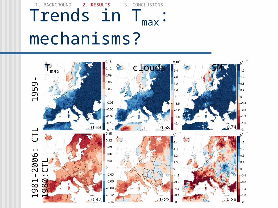
Trends in Tmax: mechanisms?

Tmax clouds SM

1981

-200

6: C

TL

1

959-

1980

:CT

L

1. BACKGROUND 2. RESULTS 3. CONCLUSIONS

no trend

Trends in Tmax: link to SM

Tmax clouds SM

1981

-200

6: I

AV

198

1-2

006

: CT

L

1. BACKGROUND 2. RESULTS 3. CONCLUSIONS

no trend

Trends in Tmax: link to SM

Aerosols are kept const. in CLM, hence (mostly) only cloud trends are the cause for Tmax trends, whereas SM act as an amplifier

Tmax clouds SM

1981

-200

6: I

AV

198

1-2

006

: CT

L

1. BACKGROUND 2. RESULTS 3. CONCLUSIONS

Trends in Tmax (extremes)

extremes mean

1981

-200

6: I

AV

1981

-200

6: C

TL

1. BACKGROUND 2. RESULTS 3. CONCLUSIONS

Trends in Tmax (extremes)

extremes mean

Stronger than those in mean

1981

-200

6: I

AV

1981

-200

6: C

TL

1. BACKGROUND 2. RESULTS 3. CONCLUSIONS

Trends in Tmax (extremes)

extremes mean

Stronger influence of SM

1981

-200

6: I

AV

1981

-200

6: C

TL

1. BACKGROUND 2. RESULTS 3. CONCLUSIONS

Conclusions

SM asymmetrically effects the PDFs of Tmax, and dampens temperature variability

1. BACKGROUND 2. RESULTS 3. CONCLUSIONS

Conclusions

SM asymmetrically effects the PDFs of Tmax, and dampens temperature variability

Reduced SM memory causes a reduction in persistence in Tmax extremes

hwdi*

1. BACKGROUND 2. RESULTS 3. CONCLUSIONS

Conclusions

1959-1980 1981-2006

SM asymmetrically effects the PDFs of Tmax, and dampens temperature variability

Reduced SM memory causes a reduction in persistence in Tmax extremes

Trends in Tmax are likely due to trends in clouds, whereas SM acts as an amplifier

hwdi*

1. BACKGROUND 2. RESULTS 3. CONCLUSIONS