robustdata fusionof multi-modalsensory information
TRANSCRIPT

Robust Data Fusion of Multi-modal Sensory
Information for Mobile Robots
Vladimır Kubelka
Center for Machine Perception, Dept. of CyberneticsFaculty of Electrical Engineering, Czech Technical University in Prague
Technicka 2, 166 27, Prague 6, Czech [email protected]
Lorenz Oswald
ETH ZurichTannenstrasse 3, 8092 Zurich, Switzerland
Francois Pomerleau
ETH ZurichTannenstrasse 3, 8092 Zurich, Switzerland
Francis Colas
ETH ZurichTannenstrasse 3, 8092 Zurich, Switzerland
Tomas Svoboda
Center for Machine Perception, Dept. of CyberneticsFaculty of Elect. Eng., CTU in Prague
Technicka 2, 166 27, Prague 6, Czech [email protected]
Michal Reinstein
Center for Machine Perception, Dept. of CyberneticsFaculty of Elect. Eng., CTU in Prague
Technicka 2, 166 27, Prague 6, Czech [email protected]
Abstract
Urban Search and Rescue missions for mobile robots require reliable state estimation sys-tems resilient to conditions given by the dynamically changing environment. We designand evaluate a data fusion system for localization of a mobile skid-steer robot intendedfor USAR missions. We exploit a rich sensor suite including both proprioceptive (inertialmeasurement unit and tracks odometry) and exteroceptive sensors (omnidirectional cameraand rotating laser rangefinder). To cope with the specificities of each sensing modality (suchas significantly differing sampling frequencies), we introduce a novel fusion scheme basedon Extended Kalman filter for 6DOF orientation and position estimation. We demonstratethe performance on field tests of more than 4.4 km driven under standard USAR condi-tions. Part of our datasets include ground truth positioning; indoor with a Vicon motioncapture system and outdoor with a Leica theodolite tracker. The overall median accuracyof localization—achieved by combining all the four modalities—was 1.2 % and 1.4 % of thetotal distance traveled, for indoor and outdoor environments respectively. To identify thetrue limits of the proposed data fusion we propose and employ a novel experimental evalua-tion procedure based on failure case scenarios. This way we address the common issues like:slippage, reduced camera field of view, limited laser rangefinder range, together with movingobstacles spoiling the metric map. We believe such characterization of the failure cases isa first step towards identifying the behavior of state estimation under such conditions. We

release all our datasets to the robotics community for possible benchmarking.
1 Introduction
Mobile robots are sought to be deployed for many tasks, from tour-guide robots to autonomous cars. Withthe rapid advance in sensor technology, it has been possible to embed richer sensor suites and extend theperception capabilities. Such sensor suites provide multi-modal information that naturally ensure perceptionrobustness, allowing also better means of self-calibration, fault detection and recovery—given that appropri-ate data fusion methods are exploited. Independently from the application, a key issue of mobile roboticsis state estimation. It is crucial for both perception, like mapping, and action, like avoiding obstacles orterrain adaptation.
In this paper, we address the problem of data fusion for localization of an Unmanned Ground Vehicle (UGV)intended for Urban Search and Rescue (USAR) missions. There has been a significant effort presented in thefield of USAR for robot localization that mostly aims for a minimal suitable sensing setup; exploiting usuallythe inertial measurements aided with either vision or laser data. Having a sufficient on-board computationalpower, we therefore aim for a richer sensors suite and hence for better robustness and reliability. Therefore,our UGV used in this work (see Figure 1) embeds track encoders, an Inertial Measurement Unit (IMU), anomnidirectional camera, and a rotating laser range-finder.
Figure 1: Picture of two USAR UGVs used for experimental evaluation (FP7-ICT-247870 NIFTi project)and a detail of the sensor setup (a PointGrey Ladybug 3 omnicamera and a rotating SICK LMS-151 laserrange finder). See Section 3.1 for more details.
Our first contribution lies in the development of a model for such multi-modal data fusion using the ExtendedKalman Filter (EKF), especially in the way we incorporate sensors with slow and fast measurement updaterates. In order to cope with such significant difference in the update rates of various sensor modalities,we concentrated the model design on integrating the slow laser and visual odometry with the faster IMUand track odometry measurements. For this purpose, we propose and investigate three different possiblemethods—one of them, the trajectory approach (see Section 4.3.3 for further details), is our contributionthat we compare it to the velocity approach, which is a common state-of-the-art practice. We show that astandard EKF designed with the velocity approach does not cope well with such significant differences in thefrequency, whether our proposed trajectory approach does.
The context of USAR missions implicitly defines challenges and limitations of our application. The envi-ronment is often unstructured (collapsed buildings) and unstable (moving objects or other ongoing changes,deformable terrain causing high slippage). Robots need to cope with indoor-outdoor transitions (changefrom confined to open spaces), bad lighting conditions with rapid changes and sometimes decreased visibility(smoke and fire). These are essentially the main challenges that come with the sensor data we process.

Therefore, our main contribution lies in the actual experimental evaluation and analysis of limits of the pro-posed filter. We review the different sensing modalities and their expected failure cases to assess the impactof possible data degradation (or outage) on the overall precision of localization. We believe that the fielddeployment of state estimation for multi-modal data fusion needs to be characterized both under standardexpected conditions as well as for case of partial or full failures of sensing modalities. Indeed, robustness tosensor data outage or degradation is a key element to the scaling up of a field robotics system. Therefore, weevaluate our filter using several hours and kilometers of experimental data validated by indoor or outdoorground truth measurements. In order to share this contribution to the robotics community, we release allthe captured datasets (including the ground truth measurements) to be used as benchmarks.1
The state of the art of sensor fusion for state estimation is elaborated in Section 2. In Section 3, we present thehardware and software used in this work before describing in details the design of our data fusion algorithm(Section 4). In Section 5, we explain our experimental evaluation including our fail-case methodology beforea discussion and conclusion (Section 6).
2 Related work
In general, the information obtained from various sensors can be classified as either proprioceptive (inertialmeasurements, joint sensors, motor or wheel encoders, etc.) or exteroceptive (Global Positioning System(GPS), cameras, laser range finder, ultrasonic sensors, magnetic compass etc.). Exteroceptive sensors thatacquire information from the environment can be also used to perceive external landmarks that are necessaryfor long-term precision in navigation tasks. In modern mobile robots, a popular solution lies usually in thecombination of a proprioceptive component in the form of Inertial Navigation System (INS) (Titterton andWeston, 1997), that captures the body dynamics at high frequency, and an external source of aiding, usingvision (Chowdhary et al., 2013) or range measurements (Bachrach et al., 2011). The key issue lies in theappropriate integration of the different characteristics of the different sensor modalities.
As it was repeatedly shown, the combination of an IMU with wheel odometry is a popular technique tolocalize a mobile robot in a dead reckoning manner. It generally allows very high sampling frequency aswell as processing rate, usually without excessive computational load. Dead reckoning can be used for shortterm navigation without any necessity of perceiving surrounding environment via exteroceptive sensors. Inreal outdoor conditions, dynamically changing environment often causes signal degradation or even outageof exteroceptive sensors. However, proprioceptive sensing, in principle, is too prone to accumulating errorsto be used as a standalone solution. Computational and environmental errors as well as errors caused bymisalignment and instrumentation cause the dead reckoning system to drift quickly with time. Moreover,motor encoders do not reflect the true path, especially heading of the vehicle, in case of frequent wheel slip.In (Yi et al., 2007) and (Anousaki and Kyriakopoulos, 2004), an improvement through skid-steer model ofa 4-wheel robot is presented, based on a Kalman filter estimating trajectory using velocity constraints andslip estimate. An alternative method appears in (Endo et al., 2007) where the IMU and odometry are usedto improve tracked vehicle navigation via slippage estimates. We addressed this problem in (Reinstein et al.,2013). Substantial effort has also been made to investigate the odometry derived constraints (Dissanayakeet al., 2001), or innovation of the motion models (Galben, 2011). Concerning all the references so far,localization of the navigated object via dead reckoning was performed only in 2D. There exist solutionsproviding real 3D odometry derived from the rover-type multi-wheel vehicle design (Lamon and Siegwart,2004). Nevertheless, the error is still about one order of magnitude higher than what we aim to achieve(below 2% of the total distance traveled).
However, if long-term precision and reliability is to be guaranteed, dead-reckoning solutions require otherexteroceptive aiding sensor systems. In the work of (Shen et al., 2011), it is shown that a very low-costIMU and odometry dead-reckoning system can be realized and successfully combined with visual odometry(VO) (Sakai et al., 2009; Scaramuzza and Fraundorfer, 2011) to produce a reliable navigation system. With
1The datasets are available as bagfiles for ROS at https://sites.google.com/site/kubelvla/public-datasets

the increasing on-board computational power, visual odometry is becoming very popular even for large-scaleoutdoor environments. Most solutions are based on the Extended Kalman filter (EKF) (Oskiper et al.,2010; Civera et al., 2010; Konolige et al., 2011; Chowdhary et al., 2013) or a dimensional-bounded EKFwith landmark classifier introduced in (Jesus and Ventura, 2012). However, in (Rodriguez F et al., 2009)it is pointed out that a trade-off between precision and execution time has to be examined. Moreover, VOdegrades due to high rotational speed movements and it is susceptible to illumination changes and lack ofsufficient scene texture (Scaramuzza and Fraundorfer, 2011).
Another typically used 6 DOF aiding source is a laser rangefinder, which is used for estimating vehiclemotion by matching consecutive laser scans and creating a 3D metric map of the environment (Suzukiet al., 2010; Yoshida et al., 2010). Examples of successful application can be found for both indoor—without IMU but combined with vision (Ellekilde et al., 2007)—as well as outdoor—relying on the IMU(Bachrach et al., 2011). As in case of the visual odometry, solutions using EKF are often proposed (Moraleset al., 2009; Bachrach et al., 2011). The most popular approach of scan matching is based on the IterativeClosest Point (ICP) algorithm first proposed by (Besl and McKay, 1992) and in parallel by (Chen andMedioni, 1991). More recently, (Nuchter et al., 2007) proposed a 6D Simultaneous Localization and Mapping(SLAM) system relying mainly on ICP. Closer to USAR applications, (Nagatani et al., 2011) demonstratedthe use of ICP in exploration missions and used a pose graph minimization scheme to handle multi-robotmapping. (Kohlbrecher et al., 2011) proposed a localization system combining a 2D laser SLAM with a3D IMU/odometry-based navigation subsystem. Combination of 3D-landmark-based SLAM and multipleproprioceptive sensors is also presented in (Chiu et al., 2013), their work aims mainly on low latency solutionwhile estimating the navigation state by means of Sliding-Window Factor Graph. The problem of utilizingseveral sensors for localization that may provide contradictory measurements is discussed in (Sukumar et al.,2007). The authors use Bayes filters to estimate sensor measurement uncertainty and sensor validity tointelligently choose a subset of sensors that contribute to localization accuracy. As opposed to the laterpublications realized in the context of SLAM, we only consider the results of the ICP algorithm as a localpose measurement similarly to (Almeida and Santos, 2013) who use the ICP algorithm to extract steeringangle and linear velocity of a car-like vehicle to update its non-holonomic model of motion. In our approach,the 3D reconstruction of the environment is considered locally coherent and neither loop detection nor errorpropagation is used.
As stated in (Kelly et al., 2012), it is the right time to address concerning issues of the state-of-the-artin long-term navigation and autonomy. In this respect, benefits and challenges of repeatable long-rangedriving were addressed in (Barfoot et al., 2012). In this context, we believe that bringing more insight intomulti-modality state estimation algorithms is an important step for long-term stability of an USAR systemevolving in a complex range of environments.
Regarding multi-modal data fusion, we built on our previous work concerning complementary filtering(Kubelka and Reinstein, 2012), odometry modeling (Reinstein et al., 2013), and design of EKF error models(Reinstein and Hoffmann, 2013), even though the later work applied to a legged robot.
3 System description
Our system aims at high state estimation accuracy while ensuring robust performance against rough terrainnavigation and obstacle traversals. We selected four modalities to achieve this goal: the inertial measure-ments (IMU ), odometry data (OD), visual odometry (VO) and laser rangefinder data (ICP) processed bythe ICP algorithm. This section explains the motion capabilities of the Search & Rescue platform and thepreprocessing computation applied to its sensors in order to extract meaningful inputs for the state estima-tion. These explanations provide a motivation for a list of states to be estimated by the EKF described inSection 4.

3.1 Mobile Robotic Platform
Figure 1 presents the UGV designed for USAR mission that we use in this paper. As described in (Kruijffet al., 2012), this platform was deployed multiple times in collaboration with various rescue services (FireDepartment of Dortmund/Germany, Vigili del Fuoco/Italy). It has two bogies linked by a differential thatallows a passive adaptation to the terrain. On each of the tracks, there are two independent flippers that canbe position-controlled in order to increase the mobility in difficult terrain. For example, they can be unfoldedto increase the support polygon which helps in overcoming gaps and being more stable on slopes. They canalso be raised to help with climbing over higher obstacles. Given that the robot was designed to operate in3D unstructured environments, the state estimation system needs to provide a 6 DOF localization.
Encoders are placed on the differential, giving the angle between the two bogies and the body; on the tracksto give their current velocity; and on each flipper to give its position with respect to its bogies. Inside thebody, vertical to the center of the robot, lies the Xsens MTi-G IMU providing angular velocities and linearacceleration along each of the three axes. The IMU data capture the body dynamics at high rate of 90 Hz.GPS is not taken into account due to the low availability of the signal indoors or in close proximity withbuilding. Magnetic compass is also easily disturbed by metallic masses, pipes, and wires, which make ithighly unreliable and hence we do not use it.
The exteroceptive sensors of the robot consist of an omnidirectional camera and a laser rangefinder. Theomnidirectional camera is the PointGrey Ladybug 3 and produces a 12 megapixels stitched omni-directionalimages at 5-6Hz. The omni-directionality of the sensor provides a stronger stability of rotation estimationat the expense of scale estimation, which would be better handled by a stereocamera. The laser rangefinderused is the Sick LMS-151 mounted on a rolling axis in front of the robot. The laser spins left and rightalternately, taking a full 360 scan at approximately 0.3Hz to create a point cloud of around 55,000 points.
3.2 Inertial data processing
Though the precision and reliability of the IMU measurements is sufficient in short term, in long termthe information provided suffers from random drift that, together with integrated noise, cause unboundederror growth. To cope with these errors all the 6 sensor biases have to be estimated (see Section 4.1 formore details). Therefore, we have included sensor biases in the state space of the proposed EKF estimator.Furthermore, correct calibration of the IMU output and its alignment with respect to the robot’s body framehas to be assured.
3.3 Odometry for skid-steer robots
Our platform is equipped with caterpillar tracks and therefore steering is realized by setting different velocitiesfor each of the tracks (skid-steering). The encoders embedded in the tracks of the platform measure theleft and right track velocities at approximatively 15Hz. However, in contradistinction to differential robots,the odometry for skid-steering vehicles has significant uncertainties. Indeed, as soon as there is a rotation,the tracks must either deform or slip significantly. The slippage is affected by many parameters includingthe type and local properties of the terrain. To keep the computation complexity low, we assume only asimple odometry model and we do not model the slippage. Instead, we take advantage of the exteroceptivemodalities in our data fusion to observe the true motion dynamics using different sources of information.Hence, the fusion compensates for cases when the tracks are slipping because the surface is slippery orbecause of an obstacle blocking the robot. Another advantage of using caterpillar tracks odometry lies inthe opportunity to exploit nonholonomic constraints. Further explanations on those constraints are given inSection 4.3.

3.4 ICP-based localization
Using as Input the current 3D point cloud, a registration process is used to estimate the pose of the robotwith respect to a global representation called Map. We used a derivation of the point-to-point ICP algo-rithm introduced by (Chen and Medioni, 1991) combined with the trimmed outlier rejection presented by(Chetverikov et al., 2002).
The implementation uses libpointmatcher2, an open-source library fast enough to handle real-time pro-cessing while offering modularity to cover multiple scenarios as demonstrated in (Pomerleau et al., 2013).The complete list of modules used with their main parameters can be found in Table 1. In more details,the configuration of the rotating laser produced a high density of points in front of the robot, which wasdesirable to predict collision but not beneficial to the registration minimization. Thus, we forced the max-imal density to 100 points per m3 after having randomly subsampled the point cloud in order to finish theregistration and the map maintenance within 2 s. We expected the error on pre-alignment of the 3D scansto be less than 0.5m based on the velocity of the platform and the number of ICP per second that was tobe executed. So we used this value to limit the matching distance. We also removed paired points with anangle difference larger than 50 to avoid the reconstruction of both sides of walls to collapse when the robotwas exploring different rooms. The surface normal vector used for the outlier filtering and for the errorminimization are computed using 20 Nearest Neighbors (NN) of every point within a single point cloud. Asfor the global map, we maintained a density of 100 points per m3 every time a new input scan was merged init. A maximum of 600,000 points were kept in memory to avoid degradation of the computation time whenexploring a larger environment than expected. However, the only output of the ICP algorithm we consideris the robot’s localization, i.e. position and orientation relative to its inner 3D point-cloud map. We do notaim at creating a globally consistent map and we do not exploit the map in any other way than for analysisof the ICP performance (no map corrections or loop closures are performed).
Table 1: Configurations of ICP chains for the NIFTi mapping applications.
Step Module Description
Input
Read. filtering SimpleSensorNoise SickLMSSamplingSurfaceNormal keep 80%, surface normals based on 20 NNObservationDirection add vector pointing toward the laserOrientNormals orient surface normals toward the obs. directionMaxDensity subsample to keep point with density of 100 pts/m3
Reg
istration
Ref. filtering - processing from the rows MapRead. filtering - processing from the rows InputData association KDTree kd-tree matching with 0.5m max. distance, ǫ = 3.16Outlier filtering TrimmedDist keep 80% closest points
SurfaceNormal remove paired normals angle > 50
Error min. PointToPlane point-to-planeTrans. checking Differential min. error below 0.01m and 0.001 rad
Counter iteration count reached 40Bound transformation fails beyond 5.0m and 0.8 rad
Map Ref. filtering SurfaceNormal Update normal and density, 20 NN, ǫ = 3.16MaxDensity subsample to keep point with density of 100 pts/m3
MaxPointCount subsample 70% if more than 600,000 points
There is one ICP-related issue observed with our platform. Although the ICP creates a locally precisemetric map, the map as whole tends to slightly twist or bend (we do not perform any loop-closure). Thisis the reason why the position and the attitude estimated by the ICP odometry collide with other positioninformation sources. Another limitation is the refresh rate of the pose measurements limited to 0.3Hz. Thisrate is far from our fastest measurement (i.e., the IMU at 90Hz), which poses a linearization problem. Forthese reasons, we investigated three different types of measurement models; see Section 4.3.3 for details.
Furthermore, the true bottleneck of the ICP-based localization lies in the way it is realized on our platform
2https://github.com/ethz-asl/libpointmatcher

and hence prone to mechanical issues. As the laser rangefinder has to be turning to provide full 3D pointcloud, in environment with high vegetation such mechanism is easily struck, causing this modality to fail.Large open spaces, indoor / outdoor transitions, or significantly large moving obstacles can also cause theICP to fail updating the metric map. Since this modality is very important, we analyzed these failure casesin Section 5.4.
3.5 Visual odometry
Our implementation of visual odometry generally follows the usual scheme (Tardif et al., 2008; Scaramuzzaand Fraundorfer, 2011). The VO computation runs solely on the robot on-board computer and estimatesthe pose at the frame rate 2-3Hz which, compared to the robot speed, is sufficient. It does search forcorrespondences (i.e., image matching) (Rublee et al., 2011), landmark reconstruction and sliding bundleadjustment (Kummerle et al., 2011; Fraundorfer and Scaramuzza, 2012), which refines the landmark 3Dpositions and the robot poses. The performance essentially depends on the visibility and variety of landmarks.The more variant landmarks are visible at more positions, the more stable and precise is the pose estimation.The process uses panoramic images constructed from spherical approximation of the Ladybug camera model.The Ladybug camera is approximated as one central camera. The error of the approximation is acceptablefor landmarks which are few meters from the robot.
The visual odometry starts with detecting and matching features in two consecutive images. We use OpenCVimplementation of the Orb keypoint detector and descriptor (Rublee et al., 2011). Only the matches, whichare distinctive above certain threshold, survive. The initial matching is supported by a guided matchingwhich uses an initial estimate of the robot movement. The robot movement is estimated by the 5-pointsolver (Li and Hartley, 2006) encapsulated in RANSAC iterations. As the error measure we use the angulardeviation of points from epipolar planes. This is less precise than the usual distance from epipolar lines.However, as we work with spherical projection we have epipolar curves. Computing angular deviationsis faster than computing distance to the epipolar curve. The movement estimate projects already knownlandmarks and we can actively search around the projection. The feature tracks are updated and associatedwith landmarks if the they pass an observation consistency test. The landmark 3D position is triangulatedfrom all possible observations and the complete estimate of landmark and robot positions are refined by abundle adjustment (Kummerle et al., 2011).
Using an almost omnidirectional camera for the robot motion estimation is geometrically advanta-geous (Brodsky et al., 1998; Svoboda et al., 1998). The scale estimation however, depends on the precisionof 3D reconstruction where the omnidirectionality does not really help. It is also important to note theomnidirectional camera we use sits very low above the terrain (below 0.5m) and directly on the robot body.This makes a huge difference compared to, e.g. (Tardif et al., 2008), where the camera is more than 2mabove the terrain and sees the ground plane much better than our camera. Estimation of the yaw angleis still well conditioned since it relies mostly on the side correspondences. The pitch estimation however,would sometimes need more landmarks on the ground plane. The pitch part of the motion induces largestdisparity of the correspondences in the front and back cameras. Unfortunately the back view is significantlyoccluded by the battery cover. This is especially problem in the street scenes where the robot moves alongthe street, see e.g., Figure 11. The front cameras see the street level better however, the uniform texture ofthe tar surface often generates only a few reliable correspondences. The search for correspondences is furthercomplicated by the tilting flippers which occlude the field of view and induce outliers. Second problemis the agility of the robot combined with relatively low frequency of the visual odometry. The robot canturn on spot very quickly, much quicker than an ordinary wheeled car. Even worse, the quick turn is theusual way how the movement direction is changed. This all makes correspondence search difficult. In thefuture versions of the visual odometry we want to improve the landmark management in order to resolve theproblem of too few landmarks surviving the sudden turn. We also think about replacing the approximatespherical model by reformulating it in a multiview model.

4 Multi-modal data fusion
The core of the data fusion system is realized by an error state EKF inspired by the work of (Weiss, 2012).The description of the multi-modal data fusion solution we propose can be divided into two parts. First isthe process error model for the EKF, that shows how we model the errors, which we aim to estimate and usefor corrections. Second part is the measurement model, that couples the sensory data coming at differentrates.
The overall scheme of our proposed approach is shown in Figure 2. Raw sensor data are preprocessed andused as measurements in the error state EKF (the FUSION block). There is no measurement rejectionimplemented; based on the assumption that fusion of several sensor modalities should deal with anomalousdata inherently—for details see Section 5 and Section 6—this however will be subjected to a future work.As apparent from the Figure 2, measurement rates significantly differ among the sensor modalities—maindifference is especially between the IMU at 90Hz and the ICP output at 0.3Hz. Having the update rate of theEKF at 90Hz the experiments have proven that this issue is crucial and has to be resolved as part of the filterdesign to ensure reliable output from the fusion process (see Section 5.3.3). In our case, this problem concernsmainly the ICP-based localization that provides measurements at very low rate of 0.3Hz—too low to capturethe motion dynamics as the IMU does (i.e. the motion dynamics spectrum gets sub-sampled). During these3 seconds, real-world disturbances (which are often non-Gaussian and difficult to model and predict, e.g.tracks slippage) accumulate. This was the motivation to investigate various ways of fusing measurementsat significantly different rates. Three proposed approaches that incorporate the ICP measurements aredescribed in the Section 4.3.3.
3-Axis
Accelerometer
ICP Matcher
Computation of
Increments in Position
and Attitude
Visual Odometry
Non-Linear State
Propagation
Comparison of
Predicted and
Actual
Measurements
EKF Error
State
Estimation
State Estimate
Correction and
Step Delay
A Priori State
Estimate
Measurement
Residual
A Posteriori
Error State
Estimate
Previous Time
Step State
Estimate
Point Cloud
(ca. 55 000
points)
Track
Odometry
3-Axis Angular
Rate Sensor
Panoramic
Image
(1600x800 px.) Computation of
Increments in Attitude
System State History for Measurement Preprocessing
IMU
@90Hz
THE MULTI-MODAL FUSION ALGORITHM
Estimates of Position, Attitude, Velocity, Angular Rate, Acceleration
and the IMU Sensor Biases
SENSORS PREPROCESSING FUSION
@90Hz
@15Hz
@2.5Hz
@0.3Hz
Figure 2: The scheme of the proposed multi-modal data fusion system (ω is angular velocity, f is specificforce (Savage, 1998), v is velocity and q is quaternion representing attitude).

4.1 Process error model
For the purpose of localization, we model our robot as a rigid body with constant angular rate and constantrate of change of velocity (ω = 0, v = const.). Presence of constant gravitational acceleration is expectedand incorporated into system model; no dissipative forces are considered.
We define four coordinate frames: R(obot) frame coincides with center of the robot, I(MU) frame representsthe Inertial Measurement Unit coordinate frame as defined by the manufacturer, O(dometry) frame representsthe tracked gear–frame, and N(avigation) frame represents the world frame. In all these frames, the North-West-Up axes convention is followed, with the x-axis pointing forwards (or to the North in the N–frame),the y-axis pointing to the left (or to the West), and the z-axis pointing upwards. Rotations about eachaxis follow the right-hand rule. The fundamental part of the system design are the differential equationsdescribing development of the states in time. The state space with the corresponding errors is defined as:
x =
pN
qRN
vR
ωR
fRbω,I
bf,I
∆x =
∆pN
δθ∆vR
∆ωR
∆fR∆bω,I
∆bf,I
(1)
where pN is position of the robot in the N–frame, qRN is unit quaternion representing its attitude, vR is
velocity expressed in the R–frame, ωR is angular rate, fR is specific force (Savage, 1998), bω,I and bf,I areaccelerometer and angular rate sensor IMU-specific biases expressed in the I–frame.
The error state ∆x is defined—following the idea of (Weiss, 2012, eq. 3.25)—as difference between the systemstate and its estimate ∆x = x − x except for attitude, where rotation error vector δθ is the vector part ofthe error quaternion δq = q ⊗ q−1 multiplied by 2; ⊗ represents quaternion multiplication as defined in(Breckenridge, 1999).
The states and the error states of the robot, modeled as a rigid body movement, propagate in time accordingto the following equations:
pN = CT(qR
N)vR ∆pN ≈ CT
(qRN)∆vR − CT
(qRN)δθ (2)
qRN =
1
2Ω(ωR)q
RN δθ ≈ −⌊ωR⌋δθ +∆ωR + nθ (3)
vR = fR − C(qRN)gN + ⌊vR⌋ωR ∆vR ≈ ∆fR − ⌊C(qR
N)gN⌋δθ + ⌊vR⌋∆ωR − ⌊ωR⌋∆vR + nv (4)
ωR = 0 fR = 0 bω,I = 0 bf,I = 0
∆ωR = nω ∆fR = nf ∆bω,I = nb,ω ∆bf,I = nb,f (5)
where derivation of the left part of (3) can be found in (Trawny and Roumeliotis, 2005, eq. 110) and theleft part of (4) is based on (Nemra and Aouf, 2010, eq. 5); the difference from the original is caused bydifferent ways of expressing attitude. The right parts of (2-4) can be derived by neglecting higher-order errorterms and by approximation of the error in attitude by the rotation error vector δθ following (Weiss, 2012,eq. 3.44). We define gN = [0, 0, g]T , n(.) are the system noise terms and Ω(ωR) in (3) is a matrix representingquaternion and vector product operation (Trawny and Roumeliotis, 2005, eq. 108). It is constructed as
Ω(ω) =
0 ω3 −ω2 ω1
−ω3 0 ω1 ω2
ω2 −ω1 0 ω3
−ω1 −ω2 −ω3 0
(6)

In (5), time derivations of angular rates and specific forces are equal to zero—usually, they are consideredrather as input than state. However, we included them into the state vector to be updated by the EKF. Theerror model equations can be expressed in compact matrix form:
∆x = Fc∆x+Gcn (7)
where Fc is continuous time state transition matrix, Gc is noise coupling matrix and n is noise vectorcomposed of all the n(.) terms; the Fc matrix is as follows:
Fc =
∅3 −CT(qR
N)
CT(qR
N)
∅3 ∅3 ∅3 ∅3
∅3 −⌊ωR⌋ ∅3 I3 ∅3 ∅3 ∅3∅3 −⌊C(qR
N)gN⌋ −⌊ωR⌋ ⌊vR⌋ I3 ∅3 ∅3
∅3 ∅3 ∅3 ∅3 ∅3 ∅3 ∅3∅3 ∅3 ∅3 ∅3 ∅3 ∅3 ∅3∅3 ∅3 ∅3 ∅3 ∅3 ∅3 ∅3∅3 ∅3 ∅3 ∅3 ∅3 ∅3 ∅3
(8)
and the Gcn term is
Gcn =
∅3 ∅3 ∅3 ∅3 ∅3 ∅3I3 ∅3 ∅3 ∅3 ∅3 ∅3∅3 I3 ∅3 ∅3 ∅3 ∅3∅3 ∅3 I3 ∅3 ∅3 ∅3∅3 ∅3 ∅3 I3 ∅3 ∅3∅3 ∅3 ∅3 ∅3 I3 ∅3∅3 ∅3 ∅3 ∅3 ∅3 I3
nθ
nv
nω
nf
nb,ω
nb,f
(9)
The noise coupling matrix describes, how particular noise terms affect the system state. Each n(·) term isa random variable with Normal probability distribution. Properties of these random variables are describedby their covariances in the system noise matrix Qc. Since they are assumed independent, the matrix Qc isdiagonal Qc = diag(σ2
θx, σ2
θy, σ2
θz, σ2
vx, σ2
vy, · · · ), where σ is standard deviation.
In order to implement the proposed model, we have to transform the continuous time equations to discretetime domain. We use the Van Loan discretization method (Loan, 1978) instead of explicitly expressing valuesof the discretized matrices. We substitute into matrix M defined by Van Loan
M =
[
−Fc GQcGT
∅ FTc
]
∆t (10)
and evaluate the matrix exponential
eM =
[
. . . F−1d Qd
∅ FTd
]
(11)
The result of the matrix exponential contains the discretized system matrix Fd in the bottom-right partand the discretized system noise matrix Qd left multiplied by the inversion of Fd in the top-right part. Thediscretized system matrix Fd can be easily extracted; Qd can be obtained by left multiplying the upper rightpart of eM by Fd.
4.2 State prediction and update using EKF
The Extended Kalman filter (Smith et al., 1962; McElhoe, 1966), is a modification of the Kalman filter(Kalman, 1960), i.e. optimal observer minimizing variances of the observed states. Since the error state EKFis used in our approach, the state of the system is expressed as sum of current best estimate (x) and some smallerror (∆x). The only difference compared to a standard EKF is that the linearised system matrices F and Qdescribe only the error state and the error state covariance propagation in time, rather than the whole stateand state covariance propagation in time. This is mainly beneficial from the computational point of view since
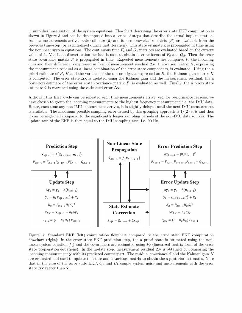
it simplifies linearisation of the system equations. Flowchart describing the error state EKF computation isshown in Figure 3 and can be decomposed into a series of steps that describe the actual implementation.As new measurements arrive, state estimate (x) and its error covariance matrix (P ) are available from theprevious time-step (or as initialized during first iteration). This state estimate x is propagated in time usingthe nonlinear system equations. The continuous time Fc and Gc matrices are evaluated based on the currentvalue of x. Van Loan discretization method is used to obtain discrete forms of Fd and Qd. Then the errorstate covariance matrix P is propagated in time. Expected measurements are compared to the incomingones and their difference is expressed in form of measurement residual ∆y. Innovation matrix H, expressingthe measurement residual as a linear combination of the error state components, is evaluated. Using the apriori estimate of P , H and the variance of the sensors signals expressed as R, the Kalman gain matrix Kis computed. The error state ∆x is updated using the Kalman gain and the measurement residual; the aposteriori estimate of the error state covariance matrix P , is evaluated as well. Finally, the a priori stateestimate x is corrected using the estimated error ∆x.
Although this EKF cycle can be repeated each time measurements arrive, yet, for performance reasons, wehave chosen to group the incoming measurements to the highest frequency measurement, i.e. the IMU data.Hence, each time any non-IMU measurement arrives, it is slightly delayed until the next IMU measurementis available. The maximum possible sampling error caused by this grouping approach is 1/(2 · 90)s and thusit can be neglected compared to the significantly longer sampling periods of the non-IMU data sources. Theupdate rate of the EKF is then equal to the IMU sampling rate, i.e. 90 Hz.
Error Update Step
Error Prediction Step
Non-Linear State
Propagation
State Estimate
Correction
Prediction Step
Update Step
Figure 3: Standard EKF (left) computation flowchart compared to the error state EKF computationflowchart (right): in the error state EKF prediction step, the a priori state is estimated using the non-linear system equation f() and the covariances are estimated using Fd (linearized matrix form of the errorstate propagation equations). In the update step, measurement residual ∆y is obtained by comparing theincoming measurement y with its predicted counterpart. The residual covariance S and the Kalman gain Kare evaluated and used to update the state and covariance matrix to obtain the a posteriori estimates. Notethat in the case of the error state EKF, Qd and Hk couple system noise and measurements with the errorstate ∆x rather than x.

4.3 Measurement error model
In general, the measurement vector y can be described as sum of measurement function h(x) of the state x
and of some random noise m due to properties of the individual sensors:
y = h(x) +m (12)
Using the function h, we can predict the measured value based on current knowledge about the system state:
y = h(x) (13)
There is a difference ∆y = y − y caused by the modeling imperfections in the state estimate as well as bythe sensor errors. This difference can be expressed in terms of the error state ∆x:
∆y = y − y = h(x)− h(x) +m
= h(x+∆x)− h(x) +m(14)
If function h is linear, (14) becomes∆y = h(∆x) +m (15)
Although the condition of linearity is not always met we still can approximate the behavior of h in someclose proximity to the current state x by a similar function h′, which is linear in elements of x such that
h(x+∆x)− h(x) ≈ h′(∆x)|x = Hx∆x (16)
where Hx is the innovation matrix projecting observed differences in measurements onto the error states.
4.3.1 IMU measurement model
The inertial measurement unit (IMU) is capable of measuring specific force (Savage, 1998) in all threedimensions as well as angular rates. The specific force measurement is a sum of acceleration and gravitationalforce, but it also contains biases—constant or slowly changing value independent of the actual acting forces—and sensor noise, which is expected to have zero mean normal probability. All the values are measured inthe I–frame.
yf,I = fI + bf,I +mf,I (17)
where yf,I is the measurement, fI is the true specific force, bf,I is sensor bias and mf,I is sensor noise.
Since the interesting value yf,I is expressed in the I–frame, we define a constant rotation matrix CIR of
R–frame to I–frame. Translation between the I– and R–frames does not affect the measured values directly;thus, it is not considered. Since the IMU is placed close to the R–frame origin, we neglect centrifugal forceinduced by rotation of R–frame and conditioned by non-zero translation between R– and I–frames. Usingthis rotation matrix, we express the measurement as:
yf,I = CIRfR + bf,I +mf,I (18)
where both fR and bf,I are elements of the system state. If we compare the measured value and the expectedmeasurement, we can express the h function, which is—in this case—equal to the h′:
yf,I − yf,I = ∆yf,I = CIRfR + bf,I − CI
R fR − bf,I +mf,I
= CIR∆fR +∆bf,I +mf,I
(19)
and hence can be expressed in Hx∆x form as
∆yf,I =[
∅3 ∅3 ∅3 ∅3 CIR ∅3 I
]
∆x+mf,I (20)
where the error state ∆x was defined in (1).

The angular rate measurement is treated identically; the output of the sensor is
yω,I = ωI + bω,I +mω,I (21)
where ωI is angular rate, bω,I is sensor bias and mω,I is sensor noise.
Similarly, the measurement residual is obtained:
yω,I − yω,I = ∆yω,I = CIR∆ωR +∆bω,I +mω,I (22)
which can be expressed in the matrix form
∆yω,I =[
∅3 ∅3 ∅3 CIR ∅3 ∅3 I
]
∆x+mω,I (23)
4.3.2 Odometry measurement model
Our platform is equipped with caterpillar tracks and therefore, steering is realized by setting different veloc-ities to each of the tracks (skid-steering). The velocities are measured by incremental optical angle sensorsat 15 Hz. Originally, we implemented a complex model introduced in (Endo et al., 2007), which exploitsangular rate measurements to model the slippage to further improve the odometry precision. However, withrespect to our sensors, no improvement was observed. Moreover, since the slippage is inherently correctedvia the proposed data fusion, we can neglect it in the odometry model, assuming only a very simple butsufficient model:
vO,x =vr + vl
2(24)
where vO,x is the forward velocity, vl and vr are track velocities measured by incremental optical sensors—thevelocities in the lateral and vertical axes are set to zero. Since the robot position is obtained by integratingvelocity expressed in R–frame, we define a rotation matrix CO
R :
vO = CORvR (25)
which expresses the vR in the O–frame.
During experimental evaluation, we observed a minor misalignment between these two frames, which canbe described as rotation about the lateral axis by approximately 1 degree. Although relatively small, thisrotation caused the position estimate in the vertical axis to grow at constant rate while the robot was movingforward. To compensate for this effect, we handle the CO
R as constant—its value was obtained by means ofcalibration. The measurement equation is then as follows:
yv,O = CORvR +mv,O (26)
where yv,O is linear velocity measured by the track odometry, expressed in O–frame. Since this relation islinear, the measurement innovation is
yv,O − yv,O = ∆yv,O =
= CORvR − CO
R vR +mv,O
= COR∆vR +mv,O
(27)
and expressed in the matrix form
∆yv,O =[
∅3 ∅3 COR ∅3 ∅3 ∅3 ∅3
]
∆x+mv,O (28)
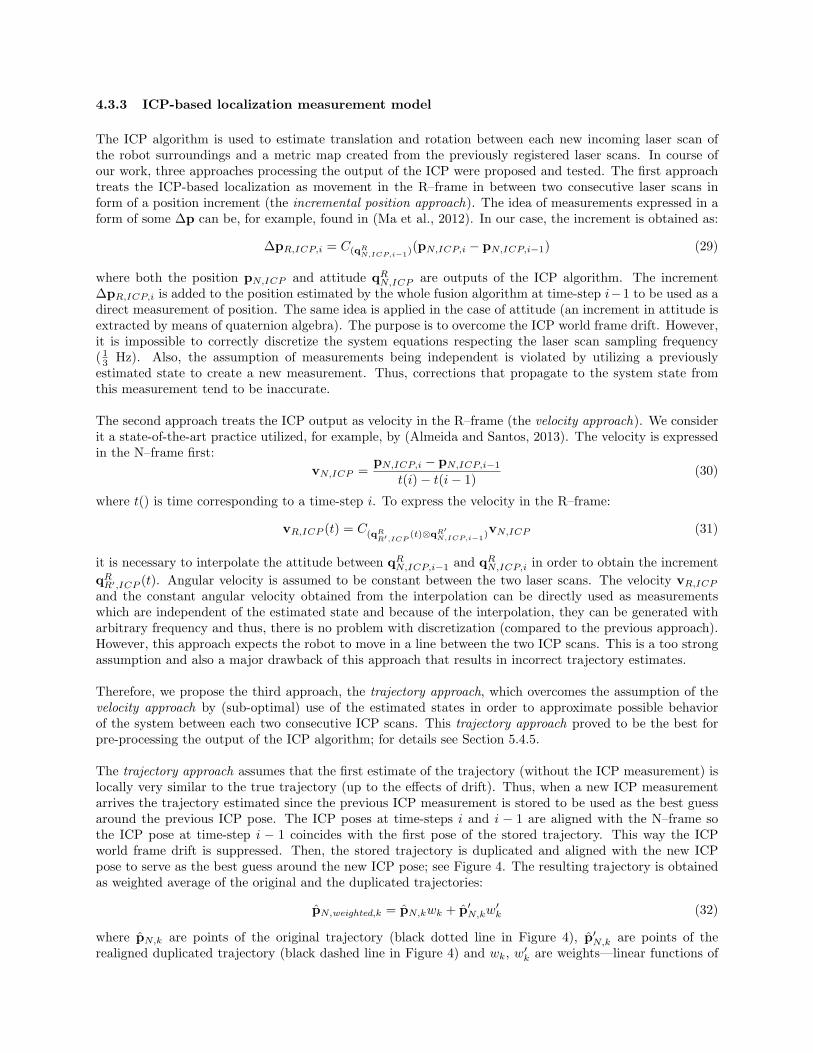
4.3.3 ICP-based localization measurement model
The ICP algorithm is used to estimate translation and rotation between each new incoming laser scan ofthe robot surroundings and a metric map created from the previously registered laser scans. In course ofour work, three approaches processing the output of the ICP were proposed and tested. The first approachtreats the ICP-based localization as movement in the R–frame in between two consecutive laser scans inform of a position increment (the incremental position approach). The idea of measurements expressed in aform of some ∆p can be, for example, found in (Ma et al., 2012). In our case, the increment is obtained as:
∆pR,ICP,i = C(qRN,ICP,i−1
)(pN,ICP,i − pN,ICP,i−1) (29)
where both the position pN,ICP and attitude qRN,ICP are outputs of the ICP algorithm. The increment
∆pR,ICP,i is added to the position estimated by the whole fusion algorithm at time-step i−1 to be used as adirect measurement of position. The same idea is applied in the case of attitude (an increment in attitude isextracted by means of quaternion algebra). The purpose is to overcome the ICP world frame drift. However,it is impossible to correctly discretize the system equations respecting the laser scan sampling frequency( 13 Hz). Also, the assumption of measurements being independent is violated by utilizing a previouslyestimated state to create a new measurement. Thus, corrections that propagate to the system state fromthis measurement tend to be inaccurate.
The second approach treats the ICP output as velocity in the R–frame (the velocity approach). We considerit a state-of-the-art practice utilized, for example, by (Almeida and Santos, 2013). The velocity is expressedin the N–frame first:
vN,ICP =pN,ICP,i − pN,ICP,i−1
t(i)− t(i− 1)(30)
where t() is time corresponding to a time-step i. To express the velocity in the R–frame:
vR,ICP (t) = C(qRR′,ICP
(t)⊗qR′
N,ICP,i−1)vN,ICP (31)
it is necessary to interpolate the attitude between qRN,ICP,i−1 and qR
N,ICP,i in order to obtain the increment
qRR′,ICP (t). Angular velocity is assumed to be constant between the two laser scans. The velocity vR,ICP
and the constant angular velocity obtained from the interpolation can be directly used as measurementswhich are independent of the estimated state and because of the interpolation, they can be generated witharbitrary frequency and thus, there is no problem with discretization (compared to the previous approach).However, this approach expects the robot to move in a line between the two ICP scans. This is a too strongassumption and also a major drawback of this approach that results in incorrect trajectory estimates.
Therefore, we propose the third approach, the trajectory approach, which overcomes the assumption of thevelocity approach by (sub-optimal) use of the estimated states in order to approximate possible behaviorof the system between each two consecutive ICP scans. This trajectory approach proved to be the best forpre-processing the output of the ICP algorithm; for details see Section 5.4.5.
The trajectory approach assumes that the first estimate of the trajectory (without the ICP measurement) islocally very similar to the true trajectory (up to the effects of drift). Thus, when a new ICP measurementarrives the trajectory estimated since the previous ICP measurement is stored to be used as the best guessaround the previous ICP pose. The ICP poses at time-steps i and i − 1 are aligned with the N–frame sothe ICP pose at time-step i − 1 coincides with the first pose of the stored trajectory. This way the ICPworld frame drift is suppressed. Then, the stored trajectory is duplicated and aligned with the new ICPpose to serve as the best guess around the new ICP pose; see Figure 4. The resulting trajectory is obtainedas weighted average of the original and the duplicated trajectories:
pN,weighted,k = pN,kwk + p′
N,kw′
k (32)
where pN,k are points of the original trajectory (black dotted line in Figure 4), p′
N,k are points of therealigned duplicated trajectory (black dashed line in Figure 4) and wk, w
′
k are weights—linear functions of

The original
trajectory estimate The original
trajectory estimate
aligned with the
second ICP pose
measurement A weighted
average resulting
trajectory
Figure 4: The principle of trajectory approach: when the new ICP measurement arrives (time-step i),trajectory estimate based on measurements other than ICP (black dotted line) is duplicated and alignedwith the incoming ICP measurement (black dashed line) and weighted average (red solid line) of these twotrajectories is computed.
time equal to 1 at time-step of associated ICP measurement and equal to 0 at time-step of the other ICPmeasurement. The resulting trajectory is used to generate the velocity measurements in the N–frame asfollows:
vN,weighted,k =pN,weighted,k − pN,weighted,k−1
t(k)− t(k − 1)(33)
where t(k) and t(k− 1) are time-steps of poses of the resulting weighted trajectory. The k denotes indexingof the fusion algorithm high-frequency samples. Velocities can be expressed in R–frame using the attitudeestimates qR
N,k:vR,weighted,k = C(qR
N,k)vN,weighted,k (34)
and can be used directly as measurement, whose projection onto the error state vector yields:
∆yv,weighted =[
∅3 ∅3 I3 ∅3 ∅3 ∅3 ∅3]
∆x+mv,weighted (35)
The velocity expressed in R–frame can be used this way as measurement, but its values for the time periodbetween two consecutive ICP outputs are known only after the second ICP measurement arrives. Thus it isnecessary to recompute state estimates for this whole time period (typically in length of 300 IMU samples),including the new velocity measurements.
To process the attitude information provided as the ICP output, we use a simple incremental approach suchthat the drift of the ICP world frame with respect to the N–frame is suppressed. To achieve this, we extractonly the increment in attitude between two consecutive ICP poses:
qRN,ICP,i = qR
R′,ICP ⊗ qR′
N,ICP,i−1 (36)
qRR′,ICP = qR
N,ICP,i ⊗(
qR′
N,ICP,i−1
)−1
(37)
where qRR′,ICP is rotation that occurred between two consecutive ICP measurements qR′
N,ICP,i−1 and qRN,ICP,i.
We apply this rotation to the attitude state estimated at time-step k′ ≡ i− 1:
yq,ICP = qRR′,ICP ⊗ qR
N,k′ (38)
To express the measurement residual, we define the following error quaternion:
δqICP,i = qRN,k ⊗ (yq,ICP )
−1(39)

where qRN,k is the attitude estimated at time-step k ≡ i. We express this residual rotation by means of
rotation vector δθICP,i
δθICP,i = 2 ~δqICP,i (40)
which can be projected onto the error state as
∆yδθ,ICP =[
∅3 I3 ∅3 ∅3 ∅3 ∅3 ∅3]
∆x+mδθ,ICP (41)
Although the ICP is very accurate in measuring translation between consecutive measurements, the attitudemeasurement is not as precise. Noise introduced in the pitch angle can cause wrong velocity estimatesexpressed in R–frame, resulting in problem described as climbing robot—the system tends to slowly drift inthe vertical axis. Since the output of the trajectory approach is velocity vR,weighted,i, applying a constraintassuming only planar motion in the R frame is fully justified, easy to implement and resolves this issue.
4.3.4 Visual odometry measurement model
As explained in Section 3.5, the visual odometry (VO) is an algorithm for estimating translation and rotationof a camera body based on images recorded by the camera. The current implementation of the data fusionutilizes only the rotation part of the motion estimated by the VO, since it is not affected by the scale.The set of 3D landmarks maintained by the VO is not in any way processed by the fusion algorithm—it isused by the VO to improve its attitude estimates internally. Similarly, the bundle adjustment ensures moreconsistent measurements, yet still, it does not enter the data fusion models.3 The way we incorporate theVO measurements is equivalent to the ICP trajectory approach, however, reduced only to the incrementalprocessing of the attitude measurements. This way, the whole VO processing block can easily be replacedby an alternative (for example by stereo vision based VO), provided the output—the estimated rotation—is available in the same way. The motivation is to have the VO measurement model independent on theVO internal implementation details. The implementation of the VO attitude aiding is identical to the ICPattitude aiding; the attitude increment is extracted and used to construct a new measurement yq,V O:
qRN,V O,i = qR
R′,V O ⊗ qR′
N,V O,i−1 (42)
qRR′,V O = qR
N,V O,i ⊗(
qR′
N,V O,i−1
)−1
(43)
where qRR′,V O is rotation that occurred between two consecutive VO measurements qR′
N,V O,i−1 and qRN,V O,i.
We apply this rotation to the attitude state estimated at time-step k′ ≡ i− 1:
yq,V O = qRR′,V O ⊗ qR
N,k′ (44)
Then, the measurement residual is expressed as error quaternion:
δqV O,i = qRN,k ⊗ (yq,V O)
−1(45)
where qRN,k is the attitude estimated at time-step k ≡ i. We express this residual rotation by means of
rotation vector δθV O,i
δθV O,i = 2 ~δqV O,i (46)
which can be projected onto the error state as
∆yδθ,V O =[
∅3 I3 ∅3 ∅3 ∅3 ∅3 ∅3]
∆x+mδθ,V O (47)
where mδθ,V O is the VO attitude measurement noise.
3The same idea applies for the ICP-based localization: although it builds an internal map, this map is independent fromour localization estimates. This would not be the case in a SLAM approach with integrated loop closures.

5 Experimental evaluation
Our evaluation procedure involves several different tests. First, we describe our evaluation methodology inSection 5.1. It covers obtaining ground truth positioning measurements for both in- and outdoors. Thenwe present and discuss our field experiments with the global behavior of our state estimation (Section 5.2).We also show two examples of typical behavior of the filter in order to give more insight on its generalcharacteristics (Section 5.3). We take advantage of them to explain the importance of the trajectory approach,compared to more standard measurement models. Finally, we analyze the behavior of the filter under failurecase scenarios involving partial or full outage of each sensory modality (Section 5.4).
5.1 Evaluation metrics
In order to validate the results of our fusion system, we need accurate measurements of part of our systemstates to confront with the proposed filter. For indoor measurements, we use a Vicon motion capture systemwith nine cameras covering more than 20m2 and giving a few millimeter accuracy at 100Hz.
For external tracking, we use a theodolite from Leica Geosystems, namely the Total Station TS15; seeFigure 5 (left). It can track a reflective prism to measure its position continuously at an average frequencyof 7.5Hz. The position precision of the theodolite is 3mm in continuous mode. However, this system cannotmeasure the orientation of the robot. Moreover, the position measured is that of the prism and not directlyof the robot, therefore we calibrated the position of the prism with respect to the robot body using thetheodolite and precise blueprints. However, the position of the robot cannot be recovered from the positionof the prism without the information about orientation. That explains why, in the validations below, we donot compare the position of the robot but the position of the prism from the theodolite and reconstructedfrom the states of our filter. With these ground-truth measurements, we use different metrics for evaluation.First, we simply plot the error as a function of time. More precisely, we consider position error, velocityerror, and attitude error and we compute it by taking the norm of the difference between the predictionmade by our filter and the reference value.
Since this metric shows how the errors evolve over time, a more condensed measure is needed to summarizeand compare the results of different versions of the filter. Therefore, we use the final position error expressedas a percentage of the total trajectory length:
erel =||pl − pref,l||
distance travelled(48)
where l is the index of the last position sample pl with the corresponding reference position pref,l.
While this metric is convenient and widely used in the literature, it is however representative only of the endpoint error regardless of the intermediary results. This can be misleading for long trajectories in confinedenvironment as the end-point might be close to the ground truth by chance. This is why we introduce, as acomplement, the average position error:
eavg(l) =
∑li=1 ||pi − pref,i||
l(49)
where 1 ≤ l ≤ total number of samples. To improve legibility of this metric in plots, we express the eavg asa function of time
e′avg(t) = eavg(l(t)) (50)
where l(t) simply maps time t to the corresponding sample l.

5.2 Performance overview of the proposed data fusion
With these metrics, we can actually evaluate the performance of our system in a quantitative way. Wedivided the tests into indoor and outdoor experiments.
5.2.1 Indoor performance
For the indoor tests, we replicated semi-structured environment found in USAR environments, includingramps, boxes, a catwalk, a small passage, etc. Figure 5 (right) shows a picture of part of the environment.Due to limitations of our motion capture set-up, this testing environment is not as large as typical indoorUSAR environments. Nevertheless, it features most of the complex characteristics that make state estimationchallenging in such an environment.
Figure 5: The experimental setup with the Leica reference theodolite for obtaining ground truth trajectory(left). Part of the 3D semi-structured environment for indoor test with motion capture ground truth (right).
For this evaluation, we recorded approximately 2.4 km of indoor data with ground truth; 28 runs representstandard conditions (765m in total), 36 runs represent failure cases of different sensory modalities inducedartificially (1613m in total). Table 2 presents the results of each combination of sensory modalities for the28 standard conditions runs; the failure scenarios are analyzed in Section 5.4 separately.
The sensory modalities combinations can be divided into two groups by including or excluding the ICPmodality; these two groups differ by the magnitude of the final position error. From this fact, we conclude thatthe main source of error is slippage of the caterpillar tracks—the VO modality in our fusion system correctsonly the attitude of the robot. Also, the results confirmed sensitivity to erroneous attitude measurementsoriginating from the sensory modalities. In this instance, VO has slightly worsen the median of the finalposition error—the indoor experiments are not long enough to make the difference between drift rates of thebare IMU+OD combination and possible VO errors that originate from incorrect pairing of image features.Nevertheless, the results are not significantly different.4 A significant improvement is brought with the ICPmodality, which compensates the tracks slippage and reduces the resulting median of the final position errorsby 50% (approximately). As expected during the filter design, fusing all sensory modalities yields the bestresult (not significantly different that without VO), with a median of 1.2% final position error; the occasionalVO attitude measurement errors are diminished by the ICP modality attitude measurement (and vice versa).
5.2.2 Outdoor performance
We ran outdoor tests in various different environments; namely a street canyon and a urban park with treesand stairs in Zurich. Figure 6 shows pictures of the environments.
4All statistical signicance results are assessed using the Wilcoxon signed-rank test with p < 0.05 testing whether the median

Final position error in % of the distance travelled
Exp. Distancetraveled [m]
Exp. duration[s]
OD, IMU OD, IMU,VO
OD, IMU,ICP
OD, IMU,ICP, VO
1 47.42 254 2.17 2.30 1.71 0.792 36.52 186 1.99 2.21 0.36 0.143 48.74 244 3.15 2.63 0.50 0.184 29.40 237 2.22 2.06 0.42 0.455 82.10 585 2.51 2.24 0.90 0.716 74.64 452 2.05 3.64 0.98 1.247 74.65 387 1.70 1.72 2.28 0.588 30.57 194 1.98 3.42 1.59 2.299 26.58 287 2.67 2.23 1.90 1.1910 26.57 236 1.53 3.94 0.77 2.1111 26.96 208 1.25 1.20 0.95 0.6612 29.13 211 1.27 1.29 0.88 0.8713 26.35 180 1.37 1.25 0.94 0.7714 40.23 240 6.58 6.70 0.88 0.9915 21.01 167 5.26 5.27 0.61 0.5716 19.04 209 5.94 5.95 0.55 0.6017 10.95 405 3.44 2.89 2.15 2.0518 8.65 238 2.87 2.77 1.36 1.3819 9.36 284 4.14 3.91 1.83 1.8520 9.02 282 2.90 3.36 2.73 2.6521 10.82 308 3.79 3.23 1.43 1.4122 9.45 237 5.36 5.45 2.66 2.6823 12.75 204 2.65 2.84 2.66 1.7924 7.81 179 1.58 1.83 2.82 3.0625 10.85 165 3.85 4.14 3.25 2.1726 10.83 163 2.36 1.84 0.62 0.6827 12.79 237 15.42 14.95 2.48 2.5328 12.07 239 28.42 27.07 2.89 2.98
Lower quartile|Median|Upper quartile 2.0|2.7|4.0 2.1|2.9|4.0 0.8|1.4|2.4 0.7|1.2|2.1
Table 2: Comparison of combinations of different modalities evaluated on indoor experiments performedunder standard conditions with the Vicon system providing ground truth in position and attitude. Finalposition error expressed in percents of the total distances traveled was chosen as metric for each experiment;the total distance of the 28 experiments was 765m, including traversing obstacles.
In those environments we recorded in total approximately 2 km, with ground truth available for 1.6 km, therest were returns from the experimental areas. These 1.6 km are split into 10 runs and, as for the indoorexperiments, Table 3) presents the results of each combination of sensory modalities for each run.
Contrary to the indoor experiments, combining all four modalities does not improve precision of localizationcompared to ICP, IMU and odometry fusion (the fusion of all is significantly worse than ICP, IMU andodometry only). Although some runs show improvement while combining all the sensory modalities (runs7, 9 and 10) or are at least comparable with the best result 0.4|0.6|1.2 (runs 4, 5 and 6), there are severalexperiments, where VO failed due to the specificities of the environments. Such failures result in erroneousattitude estimates significantly exceeding expected VO measurement noise and compromising localizationaccuracy of the fusion algorithm. The reasons for failures are described in the Section 5.4 together withother failure cases. Since we did not artificially induce these VO failures as we did in the case of theindoor experiments, we do not exclude these runs from the performance evaluation in Table 3—we considersuch environments standard for USAR. Moreover, we treat them as another proof of the fusion algorithmsensitivity to erroneous attitude measurement originating both from VO and ICP modalities and address
of correlated samples is different.

Figure 6: Pictures of the outdoor environments in Zurich. Left: street canyon, right: urban park.
Final position error in % of the distance travelled
Experiment Distancetraveled [m]
Exp.duration [s]
OD, IMU OD, IMU,VO
OD, IMU,ICP
OD, IMU,ICP, VO
1: basement 1 120.62 825 2.08 26.61 1.83 17.842: basement 2 175.67 853 1.37 12.53 2.42 5.913: hallway straight 159.42 738 1.10 20.48 0.43 12.224: street 1 135.18 584 2.78 0.72 0.24 0.625: street 2 259.86 992 9.74 0.80 0.26 0.806: park big loop 145.31 918 2.65 2.66 1.03 1.767: park small loop 88.20 601 1.94 1.60 1.25 0.978: park straight 99.29 560 1.20 20.18 0.62 11.509: 2 floors 238.28 1010 9.10 0.62 0.58 0.4310: 2 floors opposite 203.23 1107 3.23 6.79 0.51 0.42
Lower quartile|Median|Upper quartile 1.4|2.4|3.2 0.8|4.7|20.2 0.4|0.6|1.2 0.6|1.4|11.5
Table 3: Comparison of combinations of different modalities evaluated on outdoor experiments performedunder standard conditions with the Leica system providing ground truth in position.
them in the conclusions and future work.
5.3 In-depth analysis of the examples of performance
In order to have more insight on the characteristics of the filter, we selected some trajectories and show moreinformation than just the final position error metric.
5.3.1 Example of data fusion performance in indoor environment
In this example we address the caterpillar tracks slippage when traversing an obstacle (Figure 7). Sincewe are looking forward to USAR missions, such environment with conditions inducing high slippage can beexpected, e.g. collapsed buildings full of debris and dust that impairs traction on smooth surfaces such asexposed concrete walls or floors, mass traffic accidents with oil spills, etc. The Vicon system was used toobtain precise position and orientation ground truth for computing the average position error developmentn time.
When traversing a slippery surface, any track odometry inevitably fails with the tracks moving with signif-icantly diminishing traction. For this reason, trajectory and state estimates resulting from the IMU+ODfusion showed unacceptable error growth; see Figure 8. The robot was operated to attempt climbing up the

yellow slippery board (Figure 7), which deteriorated the traction to the point the robot was sliding backdown with each attempt to steer. Because of the slippage, it failed to reach the top. Then, it was drivenaround the structure and up, to further slowly slip down the slope backwards, with the tracks moving forwardto spoil traction. The effect of the slippage on the OD is apparent from the purple line in Figure 8. Thecorresponding average position error of the bare combination of IMU+OD starts to build up as soon as therobot enters the slippery slope. At 75 seconds, the IMU+OD has already an error of 0.5 m and finishes at200 sec at an error of 4.4 m (outside Figure 8). Without exteroceptive modalities this problem is unsolvableand as expected, including these modalities significantly improves the localization accuracy; the final averageposition error is only 0.14 m for the IMU+OD+VO+ICP combination. The resulting state estimates forcombination of all modalities are shown in Figure 9 and 10. Figure 9 depicts position estimates (the upperleft quarter) with the reference values. The difference between the estimate and the reference is plotted inthe bottom left quarter; similarly, the right half of the figure displays the velocity estimate. In the left partof the Figure 10, the attitude estimate expressed in Euler angles is shown with its error compared to theVicon reference. The right part of this figure demonstrates estimation of the sensor biases, which are part ofthe system state. Note, that the biases in angular rates are initialized to values obtained as the mean of an-gular rate samples measured when the robot stays stationary before each experiment—short self-calibration.Concluded, adding the exteroceptive sensor modalities—as proposed in our filter design—compensated theeffect caused by high slippage shown in this example as shown by the shape of trajectories and the averageposition error.
Figure 7: The 3D structure for testing of obstacle traversability shown a metric map created by ICP.
5.3.2 Example of data fusion performance in outdoor environment
This outdoor experiment took place on the Clausiusstrasse street (nearby ETH in Zurich) (Figure 11) andthe purpose was testing the exteroceptive modalities (the ICP and the VO) in open urban space. In thisstandard setting, both the ICP and the VO are expected to perform reasonably well, though the ICP—compared to a closed room—is missing a significant amount of spatial information (laser range is limitedapproximately to 50 meters, no ceiling etc.). The Leica theodolite was used to obtain the ground truthposition during this experiment (Figure 5).
The results are shown in Figures 12 and 13, demonstrating the improvement of performance when includingmore modalities up to the full setup. The basic dead-reckoning combination (IMU+OD) showed clearlydrift in the yaw angle caused by accumulating error due to angular rate sensor noise integration (see thepurple trajectory in the left part of Figure 12). By including the VO attitude measurements (resultingin IMU+OD+VO) the drift was compensated. Though the VO is not in fact completely drift-free, theperformance is clearly better than the angular rate integration—it is rather the scale of the trajectorythat matters. The IMU+OD+VO modality combination suffered from inaccurate track odometry velocitymeasurements (the green line in Figure 12), but this problem was resolved by including the ICP modalityinto the fusion scheme. The IMU+OD+ICP+VO combination proved to provide the best results; see theaverage position error plot in Figure 12 (right). The attitude estimates and estimates of the sensor biases

02
46
0
5
10
-5
0
5
X[m]
Y[m]
Z[m
]
0 2 4
-2
0
2
4
6
8
10
12
14
X[m]
Y
[m]
Vicon reference
Fusion of IMU, OD
Fusion of IMU, OD, ICP
Fusion of IMU, OD, ICP, VO
50 100 150 2000
0.05
0.1
0.15
0.2
0.25
0.3
0.35
0.4
0.45
0.5
Time[s]
Av
erag
e p
osi
tio
n e
rro
r[m
]
Fusion of IMU, OD
Fusion of IMU, OD, ICP
Fusion of IMU, OD, ICP, VO
Figure 8: Trajectories obtained by fusing different combinations of modalities during the indoor experimenttesting obstacle (depicted in Figure 7) traversability under high slippage (left, middle); development of theaverage position error (right).
0 50 100 150 200-2
0
2
4
6
Po
siti
on
[m]
0 50 100 150 200-1
-0.5
0
0.5
1
Vel
oci
ty[m
s-1]
X
Y
Z
Vicon
reference
0 50 100 150 2000
0.1
0.2
0.3
0.4
Po
siti
on
err
or[
m]
Time [s]0 50 100 150 200
0
0.5
1
Vel
oci
ty e
rro
r[m
s-1]
Time[s]
Figure 9: The corrected position (top left) and velocity estimates (top right) for the IMU+OD+ICP+VOcombination corresponding to the trajectory in Figure 8 (testing obstacle traversability). Errors in positionand velocity are obtained as norm of difference between the Vicon reference and the corresponding state ateach time-step (bottom left, bottom right). The Vicon reference for both position and velocity is shown inblack.
are shown in Figure 14.

0 50 100 150 200-50
0
50R
oll
,Pit
ch
[°]
0 50 100 150 200-200
0
200
Yaw
[°]
Roll
Pitch
Yaw
0 50 100 150 2000
5
10
Att
itu
de e
rro
r[°]
Time [s]
0 50 100 150 200
-0.02
0
0.02
Sp
ecif
ic f
orc
e b
ias[
ms-2
]
0 50 100 150 200
0
10
20x 10
-3
An
gu
lar
rate
bia
s[s-1
]
Time[s]
X
Y
Z
Figure 10: The corrected attitude estimates (top left) for the full multi-modal combinationIMU+OD+ICP+VO corresponding to the trajectory shown in Figure 8 (testing obstacle traversability).Errors in attitude are obtained as the difference between the Vicon reference and the corresponding state ateach time-step (bottom left). Estimated biases for the specific forces (top right) and angular rates (bottomright).
Figure 11: An example of trajectory driven by the robot over the Clausiusstrasse street.
5.3.3 Evaluation of the measurement model
We claim that a standard measurement model—as usually used for measurements coming at comparablefrequency—is not well suitable for measurements with significant differences in sampling frequencies as wellas in values, which correspond to the same state observed. This is crucial, when the difference in statesobtained from the IMU or the OD at high frequency is very large compared to the measurements providedby the ICP or the VO sensory modalities at relatively low frequency—such as in case of high slippage.
Table 4) shows the overall comparison of the three measurement models we evaluated for fusing the ICP andthe VO sensory modalities in the filter. Figure 15 presents a typical example of trajectory reconstructed byall the three measurement approaches we introduced in Section 4.3.3. The velocity approach—the state-of-the-art practice—that considers those information as relative measurements, is the least precise, with the

0
20
40
60
80
-40
-20
0
20
40
60
-10123
X[m]
Y[m]
Z[m
]Leica reference
Fusion of IMU, OD
Fusion of IMU, OD, VO
Fusion of IMU, OD, ICP, VO
0 500 10000
1
2
3
4
5
6
7
8
9
Time[s]
Av
erag
e p
osi
tio
n e
rro
r[m
]
Figure 12: Trajectories obtained by fusing different combinations of modalities during the outdoor experimentwith Leica reference system (left) and the corresponding average position error in time (right).
0 200 400 600 800 1000-50
0
50
100
Time[s]
Po
siti
on
[m]
Leica reference
0 100 200 300 400 500 600 700 800 900 1000-0.4
-0.2
0
0.2
0.4
Vel
oci
ty[m
s-1]
Time[s]
X
Y
Z
0 200 400 600 800 10000
0.5
1
1.5
2
Po
siti
on
err
or[
m]
Time[s]
Figure 13: The position and velocity estimates (top left and bottom respectively) for the IMU+OD+ICP+VOcombination corresponding to the outdoor trajectory in Figure 12; errors in position obtained as norm ofdifferences between the Leica reference and the corresponding state at each time-step (top right).
highest average position error; see Figure 15 (right). This is due to the corner cutting behavior emphasizedin Figure 15 (middle). The incremental position approach performs reasonably well in indoor environments,which are well -conditioned for the ICP and the VO sensory modalities—especially the ICP algorithm isreally precise as there are enough features to unambiguously fix all degrees of freedom. On the other hand,
0 200 400 600 800 1000-6-4-2024
Roll[°]
0 200 400 600 800 1000
-10
0
10
Pitch[°]
0 200 400 600 800 1000
-100
0
100
Yaw[°]
Time[s]
0 200 400 600 800 1000-0.04
-0.02
0
Sp
ecif
ic f
orc
e b
ias[
ms-2
]
0 200 400 600 800 1000-0.01
0
0.01
0.02
0.03
An
gu
lar
rate
bia
s[s-1
]
Time[s]
X
Y
Z
Figure 14: The attitude estimates (left) for the IMU+OD+ICP+VO combination corresponding to theoutdoor trajectory in Figure 12; biases estimated for the specific forces (top right) and angular rates (bottomright).
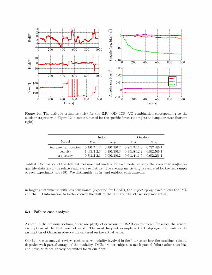
Indoor OutdoorModel erel eavg erel eavg
incremental position 0.4|0.7|1.2 0.1|0.1|0.2 0.8|1.5|11.0 0.7|2.4|6.1velocity 1.0|1.3|2.3 0.1|0.1|0.3 0.9|1.8|12.2 0.8|2.5|6.1trajectory 0.7|1.2|2.1 0.0|0.1|0.2 0.6|1.4|11.5 0.6|2.2|6.1
Table 4: Comparison of the different measurement models; for each model we show the lower|median|higherquartile statistics of the relative and average metrics. The average metric eavg is evaluated for the last sampleof each experiment, see (49). We distinguish the in- and outdoor environments.
in larger environments with less constraints (expected for USAR), the trajectory approach allows the IMUand the OD information to better correct the drift of the ICP and the VO sensory modalities.
5.4 Failure case analysis
As seen in the previous sections, there are plenty of occasions in USAR environments for which the genericassumptions of the EKF are not valid. The most frequent example is track slippage that violates theassumption of Gaussian observation centered on the actual value.
Our failure case analysis reviews each sensory modality involved in the filter to see how the resulting estimatedegrades with partial outage of the modality. IMUs are not subject to much partial failure other than biasand noise, that are already accounted for in our filter.

0 50 100 1500
0.05
0.1
0.15
0.2
0.25
Av
erag
e p
osi
tio
n e
rro
r[m
]
Time[s]
-1 0 1
-1
0
1
2P
osi
tio
n Y
[m]
Position X[m]
1 1.5 2
1.6
1.8
2
2.2
2.4
2.6
Po
siti
on
Y[m
]Position X[m]
Vicon reference
Incremental position approach
Velocity approach
Trajectory approach
Figure 15: Comparison of effects of the three different ICP aiding approaches on the estimated trajectory(left, middle) and on the average position error (right). Note the corner cutting effect of the velocity approach.
5.4.1 Robot slippage and sliding
A typical failure case of the odometry modality is significant slippage. Small slippage occurs routinely whenturning skid-steer robots and is usually accounted for by the uncertainty in the odometry model. However,on surfaces like ice, or inclined wet or smooth surfaces, stronger slippage can occur. Stronger slippages orsliding are outliers of the odometry observation model. IMU, ICP and VO sensory modalities are not affectedin such a case. In order to simulate such a situation, we placed the robot on a trolley and moved it manually.
Figure 16 shows both the trajectory from the top (top-left plot) and the comparison between the fusion ofall four sensory modalities and the fusion of only IMU+OD. We can see that the latter wrongly estimates nomotion whereas the fusion of all modalities correctly estimates the trajectory. The failure of the partial filtercan be explained by the low acceleration of the platform during the test. As the IMU acceleration signal isquite noisy, confidence on the IMU cannot compensate for the odometry modality asserting an absence ofmotion.
It should be noted that such a failure of the odometry modality does not lead to a failure of our completefilter.
5.4.2 Partial occlusion of visual field of view
Partial occlusion, overexposure, or projections of dirt on the camera could lead to faulty estimation of themotion by the VO. In order to test this situation, we occluded one of the cameras of the omnicamera (seeFigure 17). Reduction of the field of view of the omnicamera causes in the vast majority of cases a reductionin the number of visual features being robustly detected by the VO. The insufficient number of features canthen cause the VO to incorrectly estimate the attitude. This information then propagates into the stateestimate and can make the fusion algorithm fail.
Figure 18 shows the result of the filter in such a case. We can see that during a first loop of the trajectory,the state estimation is correct. Then, lacking a sufficient number of features, the VO computes an erroneousestimate and the final state estimate degenerates. On the contrary, by leaving out the visual odometry, thestate estimation would continue to perform satisfactorily.
It is to be noted that more than the portion of the field of view occluded, it is the number, quality anddistribution of features that matters. One typical way to prevent this issue is to monitor the number of

0 50 100 150 200-2
0
2
4
Po
siti
on
X[m
]
0 50 100 150 200-2
0
2
4
Po
siti
on
Y[m
]
0 50 100 150 200-0.05
0
0.05
Po
siti
on
Z[m
]
Time[s]
Vicon reference
Fusion of IMU, OD
Fusion of IMU, OD, ICP, VO
0 1 2 3-1
0
1
2
3
X[m]
Y[m
]
0 100 2000
1
2
Time[s]
Av
erag
e p
osi
tio
n
e
rro
r[m
]
Figure 16: Test trajectory for robot slippage. Black line: ground-truth; red solid line: state estimate with allfour modalities; green dashed line: IMU and odometry fusion. Top left: top view of the trajectory; bottomleft: average error as a function of time; top, middle, bottom right: evolution of x, y, z coordinate.
Figure 17: Picture from the partially occluded omnicamera. Notice the dark rectangle in the middle

-3 -2 -1 0 1 2 3
-3
-2
-1
0
1
2
3
X[m]
Y[m
]
Vicon reference
Fusion of IMU, ICP, OD, VO
100 110 120 130 1400.03
0.04
0.05
0.06
0.07
0.08
0.09
0.1
0.11
0.12
Time[s]
Av
erag
e p
osi
tio
n e
rro
r[m
]
Fusion of IMU, ICP, OD
Fusion of IMU, ICP, OD, VO
105 110 115 120 125 130 135 140-10
0
10
Roll[°]
105 110 115 120 125 130 135 140-505
10
Pitch[°]
105 110 115 120 125 130 135 140-200
0
200
Yaw[°]
Time[s]
Vicon reference
Fusion of IMU, ICP, OD
Fusion of IMU, ICP, OD, VO
Figure 18: Trajectory reconstruction with partial omnicamera occlusion. Black line: ground truth; Solid redline: state estimate with all four modalities; Dashed green line: state estimate excluding visual odometry;Black arrow: visual odometry failure. Top left: top view of the trajectory; Top right: average position erroraround visual odometry failure; Bottom: attitude estimated along the trajectory.

-3 -2 -1 0 1
-4
-2
0
2
4
6
8
X[m]
Y[m
]
Vicon reference
Raw ICP output
-20
2-5
0
5
10
0
1
2
X[m]
Y[m]
Z[m
]
Vicon reference
Fusion of IMU, OD, VO
Fusion of IMU, OD, ICP, VO
100 200 3000
0.1
0.2
0.3
0.4
0.5
0.6
0.7
0.8
0.9
1
Time[s]
Av
erag
e E
rro
r[m
]
Figure 19: Trajectory estimates in case of low ICP frequency. Black line: ground truth; cyan line: positionsestimated by ICP alone; red line: state estimate with all four modalities; green dashed line: state estimateexcluding ICP measurements. Left: top view; middle: 3D view; right: average position error.
features and eventually their distribution in the field of view—our VO tries to have corresponding featuresspread over the whole image. As Figure 18 shows, even with the partial occlusion of the field of view, theVO performed correctly during most of the trial. This observation holds also for too dark or over-exposedimages.
5.4.3 Temporary laser scanner outage
As demonstrated above, our trajectory approach to fusion of ICP measurements is able to cope with therelatively low frequency of laser scanning. As the laser is moving, it can be blocked in case of collision orhigh vibration of the platform (safety precaution at the level of the motor controller). When this happens,it is necessary to initiate a recalibration procedure that can take around 30 s.
We simulated this situation by throttling the laser point clouds, which resulted in ICP measurement outagesof up to 40 s. Figure 19 shows the trajectory estimates for this test. On the left the cyan polygon showsthe position estimates of ICP linked by straight lines (no filtering). It is to be noted that in this case, thepositions are accurate compared to the ground-truth but of very low sampling rate. We can see in the middleand right graphs that the filter estimates degrade gracefully. There is some drift, mostly along elevation dueto slippage, but even with this low frequency, the ICP measurements help correcting the state estimates overjust the IMU, odometry and visual odometry.
5.4.4 Moving obstacle and limited laser range
Unlike the cameras, laser range sensors are not sensitive to illumination conditions. On the other hand, theyhave a limited sensor range which can induce a lack of points in large environments. Close range obstaclesmight then be the dominant cluster of points and hence the ICP registration might converge to a wronglocal minimum, following the motion of the obstacles.
In order to test this situation, we artificially limited the range of the laser range sensor to 2m. This is similarto heavy smoke or dust scenarios that can arise in USAR conditions. This prevents the laser to observe the

-0.50 0.5
11.5
-0.50
0.51
1.5
0
0.5
1
X[m]Y[m]
Z[m
]
Vicon reference
ICP position
50 100 1500
0.1
0.2
Time[s]
Av
erag
e p
osi
tio
n
er
ror[
m]
Fusion of IMU, OD, VO
Fusion of IMU, OD, VO, ICP
50 100 1500
0.5
1
1.5
Po
siti
on
X[m
]
50 100 150
-0.50
0.51
1.5
Po
siti
on
Y[m
]
50 100 1500
0.2
0.4
0.6
Po
siti
on
Z[m
]
Time[s]
Vicon reference
Fusion of IMU, OD, VO
Fusion of IMU, OD, VO, ICP
ICP position
Figure 20: Trajectory estimates in case of moving obstacle in reduced field of view. Solid black line: groundtruth; solid red line: state estimate with all four modalities; dashed green line: state estimate excluding ICPmeasurements; cyan line: position estimated by ICP alone; black arrow: start of moving obstacle. Top left:3D view; bottom left: average error as a function of time; right: x, y, and z coordinates as a function oftime.
walls and the ceiling that are, indoors, usually the strongest cues for correct point cloud registration.
Additionally, we used a large board to simulate a moving obstacle of significant size. This caused the ICPto drift, following the motion of the board.
Figure 20 shows the result of the filter compared to ground truth. We can see that when the large obstaclestarts to move, the estimate of the ICP drifts with it. As a consequence the whole filter drifts as well. Thisis analogous to the slippage situation, in which the ICP modality compensates the combined estimate of theother three modalities. Using the omnicamera information not only as visual compass but also as a completevisual odometry modality would probably allow to make the difference between those two situations.
5.4.5 Map deformation
As explained above, the ICP map is not globally optimized. This means that the map might have some largescale deformations due to the accumulation of small errors. We were able to observe this particularly in along corridor that we used to assess the impact of map deformation on the state estimate.
Figure 21 shows an instance of the deformed map. We drove along two superposed corridors over two floors.We can see that both ends of the corridor are not aligned: the ground plane of the blue end has a roll angleof several degrees compared to the red end. We used the theodolite system to acquire ground truth on theupper floor.
Figure 22 shows the impact of map deformation on the state estimate. The top graph shows that even if theICP estimate is erroneous, the full filter maintains a correct, drift-free estimate. The bottom graph comparesthe estimate of the roll angle between ICP only and the fusion. It clearly shows the drift in roll of the ICPestimate and the lack of impact it has on the fusion. The difference with previous failure case lies on thekind of drift. The drift of the roll angle can be compensated for by the IMU, especially the accelerometer.On the other hand, the drift in position of previous failure case is not observable by the other modalities.

Figure 21: Deformed point cloud map created by ICP. The points are colored alongside the corridor fromred (initial position) to blue. Left: front view; top right: side view; bottom right: top view.
0 200 400 600 800 1000 1200-20
0
20
Roll[°]
Time[s]
Fusion of IMU, OD, ICP, VO
Raw ICP attitude
-70 -60 -50 -40 -30 -20 -10 0 10
-40-20
0
-10
-5
0
X[m]
Y[m]
Z[m
]
Leica reference
Fusion of IMU, OD, ICP, VO
Raw ICP position
Figure 22: Trajectory estimates in case of map deformation. Solid black line: ground truth; solid red line:state estimate with all four modalities; cyan line: position estimated by ICP alone. Top: side view; bottom:roll angle along the trajectory.

6 Conclusion
We designed and evaluated a multi-modal data fusion system for state estimation of a mobile skid-steer robotintended for Urban Search and Rescue missions. USAR missions often involve in- and outdoor environmentswith challenging conditions like slippage, moving obstacles, bad or changing light conditions, etc. In orderto cope with such environment, our robot is equipped with both proprioceptive (IMU, tracks odometry) andexteroceptive (laser rangefinder, omnidirectional camera) sensors. We designed such a data fusion scheme inorder to adequately include measurements from all these four modalities with order of magnitude differencein update frequency from 90Hz to 1
3 Hz.
We tested our algorithm on approximately 4.4 km of field tests (over more than 9 hours of data) both in-and outdoors. In order to have precise quantitative analysis, we recorded ground truth using either aVicon motion capture system (indoors) or a Leica theodolite tracker (outdoors). This way we proved thatour scheme is a significant improvement upon standard approaches. Combining all four modalities: IMU,tracks odometry, visual odometry and ICP-based localization, we achieved precision in the total distancedriven of 1.2% error in the indoor environment and 1.4% error in the outdoor environment. Moreover,we characterized the reliability of our data fusion scheme against sensor failures. We designed failure casescenarios according to potential failures of each sensory modality that are likely to occur during real USARmissions. In course of this testing, we evaluated robustness with respect to: heavy slippage (odometry failurecase), reduction of field of view of the omnicamera (visual odometry failure case), and reduction of the laserrangefinder together with large moving obstacles spoiling the created metric map (ICP-based localizationfailure case).
While our filter demonstrates good accuracy during our field tests and is robust against some of the failuresexpected in USAR, there is still a space for improvement—the need for an automatic failure detection andresolution. Exploring different methods of detecting anomalous measurements and rejecting them in orderto improve the overall performance is one of the ways, but it is currently left for future work. Furthermore,developing a visual odometry solution capable of providing also estimates of scaled translation is anothertopic for the future.
It is not surprising that combining more modalities yields more precision. But we were able to show thatif such a rich multi-modal system is well designed, it will perform reasonably well even in cases, whereother systems exploiting fewer modalities fail completely. We describe how to design such system using thecommonly used EKF. In this way we contribute by proposing and comparing three different approaches totreat the ICP measurements; out of which the trajectory approach proved to perform best.
To contribute to the robotics community, we release our datasets used in this paper, including the groundtruth measurements from Vicon and Leica systems.
Acknowledgments
The research presented here was supported by the European Union FP7 Programme under the NIFTi project(No. 247870; http://www.nifti.eu) and the TRADR project (No. 609763; http://www.tradr-project.eu). Francois Pomerleau was supported by a fellowship from the Fonds quebecois de recherche sur lanature et les technologies (FQRNT). Vladimir Kubelka was supported by the Czech Science Foundation(Project Registration No. 14-13876S). We would like to thank the anonymous reviewers for their constructivesuggestions that greatly improved the manuscript.

References
Almeida, J. and Santos, V. M. (2013). Real time egomotion of a nonholonomic vehicle using lidar measure-ments. Journal of Field Robotics, 30(1):129–141.
Anousaki, G. and Kyriakopoulos, K. J. (2004). A dead-reckoning scheme for skid-steered vehicles in out-door environments. In Robotics and Automation (ICRA), 2004. Proceedings of the IEEE InternationalConference on, pages 580–585.
Bachrach, A., Prentice, S., He, R., and Roy, N. (2011). RANGE—Robust autonomous navigation in GPS-denied environments. Journal of Field Robotics, 28(5):644–666.
Barfoot, T., Stenning, B., Furgale, P., and McManus, C. (2012). Exploiting reusable paths in mobile robotics:Benefits and challenges for long-term autonomy. In Computer and Robot Vision (CRV), 2012 NinthConference on, pages 388–395.
Besl, P. and McKay, H. (1992). A method for registration of 3-D shapes. Pattern Analysis and MachineIntelligence, IEEE Transactions on, 14(2):239–256.
Breckenridge, W. G. (1999). Quaternions - proposed standard conventions. Technical report, JPL.
Brodsky, T., Fermueller, C., and Aloimonos, Y. (1998). Directions of motion fields are hardly ever ambiguous.International Journal of Computer Vision, 26(1):5–24.
Chen, Y. and Medioni, G. (1991). Object modeling by registration of multiple range images. In Robotics andAutomation (ICRA), 1991. Proceedings of the IEEE International Conference on, pages 2724–2729.
Chetverikov, D., Svirko, D., Stepanov, D., and Krsek, P. (2002). The Trimmed Iterative Closest Pointalgorithm. In Pattern Recognition, 2002. Proceedings of the 16th International Conference on, pages545–548.
Chiu, H.-P., Williams, S., Dellaert, F., Samarasekera, S., and Kumar, R. (2013). Robust vision-aided naviga-tion using sliding-window factor graphs. In Robotics and Automation (ICRA), 2013 IEEE InternationalConference on, pages 46–53.
Chowdhary, G., Johnson, E. N., Magree, D., Wu, A., and Shein, A. (2013). GPS-denied Indoor and OutdoorMonocular Vision Aided Navigation and Control of Unmanned Aircraft. Journal of Field Robotics,30(3):415–438.
Civera, J., Grasa, O. G., Davison, A. J., and Montiel, J. M. M. (2010). 1-Point RANSAC for extendedKalman filtering: Application to real-time structure from motion and visual odometry. Journal of FieldRobotics, 27(5):609–631.
Dissanayake, G., Sukkarieh, S., Nebot, E., and Durrant-Whyte, H. (2001). The aiding of a low-cost strap-down inertial measurement unit using vehicle model constraints for land vehicle applications. IEEETransactions on Robotics and Automation, 17(5):731–747.
Ellekilde, L.-P., Huang, S., Miro, J. V., and Dissanayake, G. (2007). Dense 3D Map Construction for IndoorSearch and Rescue. J. Field Robotics, 24(1-2):71–89.
Endo, D., Okada, Y., Nagatani, K., and , K. (2007). Path following control for tracked vehicles based onslip-compensating odometry. In Proc. IEEE/RSJ Int. Conf. Intelligent Robots and Systems IROS 2007,pages 2871–2876.
Fraundorfer, F. and Scaramuzza, D. (2012). Visual Odometry : Part II: Matching, Robustness, Optimization,and Applications. Robotics Automation Magazine, IEEE, 19(2):78–90.
Galben, G. (2011). New Three-Dimensional Velocity Motion Model and Composite Odometry–Inertial Mo-tion Model for Local Autonomous Navigation. IEEE Transactions on Vehicular Technology, 60(3):771–781.

Jesus, F. and Ventura, R. (2012). Combining monocular and stereo vision in 6d-slam for the localizationof a tracked wheel robot. In Safety, Security, and Rescue Robotics (SSRR), 2012 IEEE InternationalSymposium on, pages 1–6.
Kalman, R. E. (1960). A new approach to linear filtering and prediction problems. Journal of basic Engi-neering, 82(1):34–45.
Kelly, J., Sibley, G., Barfoot, T., and Newman, P. (2012). Taking the Long View: A Report on Two RecentWorkshops on Long-Term Autonomy. Robotics & Automation Magazine, IEEE, 19(1):109–111.
Kohlbrecher, S., Stryk, O. V., Meyer, J., and Klingauf, U. (2011). A flexible and scalable slam system withfull 3d motion estimation. In Safety, Security, and Rescue Robotics (SSRR), 2011 IEEE InternationalSymposium on, pages 155–160.
Konolige, K., Agrawal, M., and Sola, J. (2011). Large-scale visual odometry for rough terrain. In Kaneko,M. and Nakamura, Y., editors, Robotics Research, volume 66 of Springer Tracts in Advanced Robotics,pages 201–212. Springer.
Kruijff, G. J. M., Janicek, M., Keshavdas, S., Larochelle, B., Zender, H., Smets, N. J. J. M., Mioch, T.,Neerincx, M. A., van Diggelen, J., Colas, F., Liu, M., Pomerleau, F., Siegwart, R., Hlavac, V., Svoboda,T., Petricek, T., Reinstein, M., Zimmerman, K., Pirri, F., Gianni, M., Papadakis, P., Sinha, A., Balmer,P., Tomatis, N., Worst, R., Linder, T., Surmann, H., Tretyakov, V., Surmann, H., Corrao, S., Pratzler-Wanczura, S., and Sulk, M. (2012). Experience in System Design for Human-Robot Teaming in UrbanSearch and Rescue. In Field and Service Robotics, pages 1–14, Matsushima, Japan.
Kubelka, V. and Reinstein, M. (2012). Complementary filtering approach to orientation estimation usinginertial sensors only. In Robotics and Automation (ICRA), 2012 IEEE International Conference on,pages 599–605.
Kummerle, R., Grisetti, G., Strasdat, H., Konolige, K., and Burgard, W. (2011). g2o: A general frameworkfor graph optimization. In Robotics and Automation (ICRA), 2011 IEEE International Conference on,pages 3607–3613. IEEE.
Lamon, P. and Siegwart, R. (2004). Inertial and 3D-odometry fusion in rough terrain - towards real 3Dnavigation. In Proc. IEEE/RSJ Int. Conf. Intelligent Robots and Systems (IROS 2004), pages 1716–1721.
Li, H. and Hartley, R. (2006). Five-point motion estimation made easy. In Pattern Recognition, 2006. ICPR2006. 18th International Conference on, volume 1, pages 630–633.
Loan, C. V. (1978). Computing integrals involving the matrix exponential. Automatic Control, IEEETransactions on, 23(3):395–404.
Ma, J., Susca, S., Bajracharya, M., Matthies, L., Malchano, M., and Wooden, D. (2012). Robust multi-sensor, day/night 6-dof pose estimation for a dynamic legged vehicle in gps-denied environments. InRobotics and Automation (ICRA), 2012 IEEE International Conference on, pages 619–626.
McElhoe, B. A. (1966). An Assessment of the Navigation and Course Corrections for a Manned Flyby ofMars or Venus. Aerospace and Electronic Systems, IEEE Transactions on, 2(4):613–623.
Morales, Y., Carballo, A., Takeuchi, E., Aburadani, A., and Tsubouchi, T. (2009). Autonomous robotnavigation in outdoor cluttered pedestrian walkways. Journal of Field Robotics, 26(8):609–635.
Nagatani, K., Okada, Y., Tokunaga, N., Kiribayashi, S., Yoshida, K., Ohno, K., Takeuchi, E., Tadokoro,S., Akiyama, H., Noda, I., Yoshida, T., and Koyanagi, E. (2011). Multirobot exploration for searchand rescue missions: A report on map building in robocuprescue 2009. Journal of Field Robotics,28(3):373–387.
Nemra, A. and Aouf, N. (2010). Robust INS/GPS Sensor Fusion for UAV Localization Using SDRE NonlinearFiltering. IEEE Sensors Journal, 10(4):789–798.

Nuchter, A., Lingemann, K., Hertzberg, J., and Surmann, H. (2007). 6D SLAM - 3D mapping outdoorenvironments. Journal of Field Robotics, 24(8-9):699–722.
Oskiper, T., Chiu, H.-P., Zhu, Z., Samarasekera, S., and Kumar, R. (2010). Multi-modal sensor fusionalgorithm for ubiquitous infrastructure-free localization in vision-impaired environments. In IntelligentRobots and Systems (IROS), 2010 IEEE/RSJ International Conference on, pages 1513–1519.
Pomerleau, F., Colas, F., Siegwart, R., and Magnenat, S. (2013). Comparing ICP Variants on Real-WorldData Sets. Autonomous Robots, 34(3):133–148.
Reinstein, M. and Hoffmann, M. (2013). Dead reckoning in a dynamic quadruped robot based on multimodalproprioceptive sensory information. IEEE Transactions on Robotics, 29(2):563–571.
Reinstein, M., Kubelka, V., and Zimmermann, K. (2013). Terrain adaptive odometry for mobile skid-steerrobots. In Proc. IEEE Int Robotics and Automation (ICRA) Conf, pages 4706–4711.
Rodriguez F, S. A., Fremont, V., and Bonnifait, P. (2009). An experiment of a 3D real-time robust visualodometry for intelligent vehicles. In Proc. 12th Int. IEEE Conf. Intelligent Transportation SystemsITSC ’09, pages 1–6.
Rublee, E., Rabaud, V., Konolige, K., and Bradski, G. (2011). ORB: An efficient alternative to SIFT orSURF. In Computer Vision (ICCV), 2011 IEEE International Conference on, pages 2564 –2571.
Sakai, A., Tamura, Y., and Kuroda, Y. (2009). An efficient solution to 6DOF localization using UnscentedKalman Filter for planetary rovers. In Proc. IEEE/RSJ Int. Conf. Intelligent Robots and Systems IROS2009, pages 4154–4159.
Savage, P. G. (1998). Strapdown inertial navigation integration algorithm design part 2: Velocity andposition algorithms. Journal of Guidance, Control, and Dynamics, 21(No. 2):208 – 221.
Scaramuzza, D. and Fraundorfer, F. (2011). Visual odometry [tutorial]. IEEE Robot Autom Mag, 18(4):80–92.
Shen, J., Tick, D., and Gans, N. (2011). Localization through fusion of discrete and continuous epipolargeometry with wheel and IMU odometry. In Proc. American Control Conf. (ACC), pages 1292–1298.
Smith, G. L., Schmidt, S. F., and McGee, L. A. (1962). Optimal filtering and linear prediction applied to amidcource navigation system for the circumlunar mission. Technical report, U.S. Government PrintingOffice.
Sukumar, S. R., Bozdogan, H., Page, D. L., Koschan, A. F., and Abidi, M. A. (2007). Sensor selection usinginformation complexity for multi-sensor mobile robot localization. In Robotics and Automation, 2007IEEE International Conference on, pages 4158–4163.
Suzuki, T., Kitamura, M., Amano, Y., and Hashizume, T. (2010). 6-DOF localization for a mobile robotusing outdoor 3D voxel maps. In Proc. IEEE/RSJ Int Intelligent Robots and Systems (IROS) Conf,pages 5737–5743.
Svoboda, T., Pajdla, T., and Hlavac, V. (1998). Motion estimation using central panoramic cameras. InIEEE International Conference on Intelligent Vehicles, pages 335–340.
Tardif, J., Pavlidis, Y., and Daniilidis, K. (2008). Monocular visual odometry in urban environments using anomnidirectional camera. In Intelligent Robots and Systems, 2008. IROS 2008. IEEE/RSJ InternationalConference on, pages 2531–2538.
Titterton, D. H. and Weston, J. L. (1997). Strapdown Inertial Navigation Technology. The Lavenham Pressltd, Lavenham, UK.
Trawny, N. and Roumeliotis, S. I. (2005). Indirect Kalman Filter for 3D Attitude Estimation - A Tutorialfor Quaternion Algebra. Technical report, University of Minnesota.

Weiss, S. M. (2012). Vision based navigation for micro helicopters. Dissertation, ETH Zurich.
Yi, J., Zhang, J., Song, D., and Jayasuriya, S. (2007). Imu-based localization and slip estimation for skid-steered mobile robots. In Proc. IEEE/RSJ Int. Conf. Intelligent Robots and Systems IROS 2007, pages2845–2850.
Yoshida, T., Irie, K., Koyanagi, E., and Tomono, M. (2010). A sensor platform for outdoor navigation usinggyro-assisted odometry and roundly-swinging 3D laser scanner. In Proc. IEEE/RSJ Int IntelligentRobots and Systems (IROS) Conf, pages 1414–1420.