robust statistics for computer vision: model fitting ...hwang/papers/hanzi_phd_thesis.pdf · robust...
TRANSCRIPT
Robust Statistics for Computer Vision:
Model Fitting, Image Segmentation and
Visual Motion Analysis
by
Hanzi Wang
B.S. (Sichuan University) 1996
M.S. (Sichuan University) 1999
A thesis submitted for the degree of
Doctor of Philosophy`
in the
Department of Electrical and Computer Systems Engineering
Monash University
Clayton Victoria 3800
Australia
February 2004

Robust Statistics for Computer Vision: Model Fitting,
Image Segmentation and Visual Motion Analysis
Copyright © 2004
by
Hanzi Wang
All Rights Reserved

i
List of Figures vii
List of Tables x
Summary xi
Declaration xv
Preface xvi
Acknowledgements xix
Dedication xxi
1. Introduction.....................................................................................................................1
1.1 Background and Motivation ....................................................................................1
1.2 Thesis Outline ..........................................................................................................6
2. Model-Based Robust Methods: A Review ....................................................................8
2.1 The Least Squares (LS) Method ..............................................................................9
2.2 Outliers and Breakdown Point ...............................................................................11
2.3 Traditional Robust Estimators from Statistics .......................................................13
2.3.1 M-Estimators and GM-Estimators ...................................................................... 13
2.3.2 The Repeated Median (RM) Estimator............................................................... 15
2.3.3 The Least Median of Squares (LMedS) Estimator............................................. 16
2.3.4 The Least Trimmed Squares (LTS) Estimator.................................................... 19
ContentsContents

ii
2.4 Robust Estimators Developed within the Computer Vision Community..............20
2.4.1 Breakdown Point in Computer Vision ................................................................ 21
2.4.2 Hough Transform (HT) Estimator....................................................................... 22
2.4.3 Random Sample Consensus (RANSAC) Estimator .......................................... 23
2.4.4 Minimize the Probability of Randomness (MINPRAN) Estimator.................. 24
2.4.5 Minimum Unbiased Scale Estimator (MUSE) and Adaptive Least kth Order
Squares (ALKS) Estimator .................................................................................. 25
2.4.6 Residual Consensus (RESC) Estimator .............................................................. 28
2.5 Conclusion .............................................................................................................30
3. Using Symmetry in Robust Model Fitting..................................................................31
3.1 Introduction............................................................................................................31
3.2 Dilemma of the LMedS and the LTS in the Presence of Clustered Outliers.........33
3.3 The Symmetry Distance.........................................................................................37
3.3.1 Definition of Symmetry ....................................................................................... 38
3.3.2 The Symmetry Distance....................................................................................... 39
3.4 The Least Trimmed Symmetry Distance (LTSD) Method....................................40
3.5 Experimental Results .............................................................................................41
3.5.1 Circle Fitting ......................................................................................................... 42
3.5.2 Ellipse fitting ......................................................................................................... 43
3.5.3 Experiments with Real Images ............................................................................ 45
3.5.4 Experiments for the Data with Uniform Outliers ............................................... 47
3.6 Conclusion .............................................................................................................48
4. MDPE: A Novel and Highly Robust Estimator .........................................................50
4.1 Introduction............................................................................................................50
4.2 Nonparametric Density Gradient Estimation and Mean Shift Method..................52
4.3 Maximum Density Power Estimator—MDPE ......................................................56
4.3.1 The Density Power (DP) ...................................................................................... 56
4.3.2 The MDPE Algorithm.......................................................................................... 57
4.4 Experiments and Analysis .....................................................................................58
4.4.1 Experiment 1......................................................................................................... 59
4.4.1.1 Line Fitting .................................................................................59
iii
4.4.1.2 Circle Fitting ...............................................................................62
4.4.1.3 Time Complexity ........................................................................63
4.4.2 Experiment 2......................................................................................................... 64
4.4.3 Experiment 3......................................................................................................... 66
4.4.4 Experiment 4......................................................................................................... 68
4.4.4.1 The Influence of the Window Radius and the Percentage of
Outliers on MDPE….. ................................................................69
4.4.4.2 The Influence of the Choice of Error Tolerance on RANSAC...70
4.4.4.3 The Relationship between the Noise Level of Signal and the
Choice of Window Radius for MDPE ........................................71
4.4.5 Experiments on Real Images ............................................................................... 72
4.5 Conclusion .............................................................................................................74
5. A Novel Model-Based Algorithm for Range Image Segmentation ................................79
5.1 Introduction............................................................................................................79
5.2 A Review of Several State-of-the-Art Methods for Range Image Segmentation..84
5.2.1 The USF Range Segmentation Algorithm.......................................................... 84
5.2.2 The WSU Range Segmentation Algorithm ........................................................ 85
5.2.3 The UB Range Segmentation Algorithm............................................................ 86
5.2.4 The UE Range Segmentation Algorithm............................................................ 87
5.2.5 Towards to Model-Based Range Image Segmentation Method ....................... 89
5.3 A Quick Version of the MDPE—QMDPE............................................................89
5.3.1 QMDPE................................................................................................................. 90
5.3.2 The Breakdown Plot of QMDPE ........................................................................ 91
5.3.3 The Time Complexity of QMDPE...................................................................... 92
5.3.4 The Influence of Window Radius on the Results of QMDPE........................... 92
5.4 Applying QMDPE to Range Image Segmentation ................................................93
5.4.1 From Estimator to Segmenter.............................................................................. 93
5.4.2 A New and Efficient Model-Based Algorithm for Range Image
Segmentation......................................................................................................... 94
5.5 Experiments in Range Image Segmentation..........................................................98
5.6 Conclusion ...........................................................................................................104

iv
6. Variable-Bandwidth QMDPE for Robust Optical Flow Calculation ....................106
6.1 Introduction..........................................................................................................106
6.2 Optical Flow Computation...................................................................................107
6.3 From QMDPE to vbQMDPE...............................................................................108
6.3.1 Bandwidth Choice .............................................................................................. 109
6.3.2 The Algorithm of the Variable Bandwidth QMDPE....................................... 109
6.3.3 Performance of vbQMDPE................................................................................ 110
6.4 vbQMDPE and Optical Flow Calculation ...........................................................111
6.4.1 Variable-Bandwidth-QMDPE Optical Flow Computation ............................. 113
6.4.2 Quantitative Error Measures for Optical Flow ................................................. 114
6.5 Experimental Results on Optical Flow Calculation.............................................114
6.6 Conclusion ...........................................................................................................116
7. A Highly Robust Scale Estimator for Heavily Contaminated Data.......................120
7.1 Introduction..........................................................................................................120
7.2 Robust Scale Estimators ......................................................................................121
7.2.1 The Median and Median Absolute Deviation (MAD) Scale Estimator ......... 122
7.2.2 Adaptive Least K-th Squares (ALKS) Scale Estimator................................... 123
7.2.3 Residual Consensus (RESC) Scale Estimator .................................................. 124
7.2.4 Modified Selective Statistical Estimator (MSSE) ............................................ 124
7.3 A Novel Robust Scale Estimator: TSSE..............................................................125
7.3.1 Mean Shift Valley Algorithm ............................................................................ 125
7.3.2 Two-Step Scale Estimator (TSSE) .................................................................... 128
7.4 Experiments on Robust Scale Estimation............................................................129
7.4.1 Normal Distribution............................................................................................ 129
7.4.2 Two-mode Distribution...................................................................................... 129
7.4.3 Two-mode Distribution with Random Outliers................................................ 130
7.4.4 Breakdown Plot................................................................................................... 130
7.4.4.1 A Roof Signal ...........................................................................130
7.4.4.2 A Step Signal ............................................................................131
7.4.4.3 Breakdown Plot for Robust Scale Estimator ............................133
7.4.4.4 Performance of TSSE ...............................................................134
7.5 Conclusions..........................................................................................................134

v
8. Robust Adaptive-Scale Parametric Model Estimation for Computer Vision .......136
8.1 Introduction..........................................................................................................136
8.2 Adaptive Scale Sample Consensus (ASSC) Estimator Algorithm ......................138
8.3 Experiments with Data Containing Multiple Structures......................................140
8.3.1 2D Examples....................................................................................................... 141
8.3.2 3D Examples....................................................................................................... 142
8.3.3 The Breakdown Plot of the Four Methods........................................................ 145
8.3.4 Influence of the Noise Level of Inliers on the Results of Robust Fitting........ 147
8.3.5 Influence of the Relative Height of Discontinuous Signals............................. 148
8.4 ASSC for Range Image Segmentation.................................................................149
8.4.1 The Algorithm of ASSC-Based Range Image Segmentation ......................... 150
8.4.2 Experiments on Range Image Segmentation.................................................... 151
8.5 ASSC for Fundamental Matrix Estimation..........................................................154
8.5.1 Background of Fundamental Matrix Estimation .............................................. 154
8.5.2 The Experiments on Fundamental Matrix Estimation ..................................... 154
8.6 A Modified ASSC (ASRC)..................................................................................157
8.6.1 Adaptive-Scale Residual Consensus (ASRC) .................................................. 157
8.6.2 Experiments......................................................................................................... 158
8.7 Conclusion ...........................................................................................................160
9. Mean shift for Image Segmentation by Pixel Intensity or Pixel Color ..................162
9.1 Introduction..........................................................................................................162
9.2 False-Peak-Avoiding Mean Shift for Image Segmentation.................................165
9.2.1 The Relationship between the Gray-Level Histogram of Image and the Mean
Shift Method........................................................................................................ 165
9.2.2 The False Peak Analysis .................................................................................... 166
9.2.3 An Unsupervised Peak-Valley Sliding Algorithm for Image Segmentation.. 169
9.2.4 Experimental Results.......................................................................................... 170
9.3 Color Image Segmentation Using Global Information and Local Homogeneity 172
9.3.1 HSV Color Space................................................................................................ 173
9.3.2 Considering the Cyclic Property of the Hue Component in the Mean Shift
Algorithm ............................................................................................................ 175
9.3.3 The Proposed Segmentation Method for Color Images................................... 175

vi
9.3.3.1 Local Homogeneity...................................................................176
9.3.3.2 Color Image Segmentation Method..........................................176
9.3.4 Experiments on Color Image Segmentation..................................................... 178
9.4 Conclusion ...........................................................................................................181
10. Conclusion and Future Work ....................................................................................183
Bibliography 184

vii
Chapter 1. Introduction 1
Figure 1.1: The OLS estimator may breakdown.....................................................................2
Figure 1.2: Examples of multiple strucutres...........................................................................3
Chapter 2. Model-Based Robust Methods: A Review 8
Figure 2.1: The types of outliers. ..........................................................................................11
Chapter 3. Using Symmetry in Robust Model Fitting 31
Figure 3.1: An example where LMedS and LTS fail to fit a circle ......................................34
Figure 3.2: LMedS searches for the “best” fit with the least median of residuals................35
Figure 3.3: Breakdown Plot of LMedS and LTS..................................................................36
Figure 3.4: Four kinds of symmetries...................................................................................39
Figure 3.5: Example of using the symmetry of the circle in the LTSD method...................42
Figure 3.6: Comparative result of the LTSD, LMedS, and LTS in circle fitting .................43
Figure 3.7: Comparison of the results of the LTSD, LTS and LMedS in ellipse fitting ......45
Figure 3.8: Fitting a mouse pad by the LTSD, LTS and LMedS methods...........................46
Figure 3.9: Fitting the ellipse in a cup by the LTSD, LTS and LMedS methods.................47
Figure 3.10: An ellipse with 40% randomly distributed outliers..........................................48
Chapter 4. MDPE: A Novel and Highly Robust Estimator 50
Figure 4.1: One example of the mean shift estimator...........................................................55
Figure 4.2: Comparing the performance of six methods .....................................................60
Figure 4.3: One example of fitting circles by the six methods. ............................................62
Figure 4.4: Experiment fitting a line with clustered outliers. ...............................................65
Figure 4.5: Breakdown plot for the six methods ..................................................................67
Figure 4.6: The influence of window radius and percentage of outliers on the results of the
MDPE. ..........................................................................................................................69
ContentsList of Figures

viii
Figure 4.7: The influence of the choice of error bound on the results of RANSAC. ...........71
Figure 4.8: The relationship between the noise level of signal and the choice of window
radius in MDPE. ...........................................................................................................72
Figure 4.9: Fitting a line by the six methods ........................................................................72
Figure 4.10: Fitting a circle edge by the six methods...........................................................73
Chapter 5. A Novel Model-Based Algorithm for Range Image Segmentation 79
Figure 5.1: The simplified 3D recognition systems..............................................................80
Figure 5.2: Breakdown plot for the QMDPE method .........................................................91
Figure 5.3: The influence of window radius on the results of the QMDPE. ........................92
Figure 5.4: The structure of the proposed range image segmentation algorithm .................95
Figure 5.5: A comparison of using normal information or not using normal information...98
Figure 5.6: Segmentation of ABW range image (test.28) ....................................................99
Figure 5.7: Segmentation of ABW range image (test.27) ..................................................100
Figure 5.8: Segmentation of ABW range image (test.13) ..................................................101
Figure 5.9: Comparison of the segmentation results for ABW range image (test.1) .........102
Figure 5.10: Comparison of the segmentation results for ABW range image (train 6)......103
Chapter 6. Variable-Bandwidth QMDPE for Robust Optical Flow Calculation 106
Figure 6.1: Comparing the performance of vbQMDPE, LS, LMedS, and LTS.................110
Figure 6.2: One example of multiple motions. ...................................................................112
Figure 6.3: The snapshot of the three image sequences .....................................................115
Chapter 7. A Highly Robust Scale Estimator for Heavily Contaminated Data 120
Figure 7.1: An example of the application of the mean shift valley method......................127
Figure 7.2: Breakdown plot of six methods in estimating the scale of a roof signal..........131
Figure 7.3: Breakdown plot of six methods in estimating the scale of a step signal. .........132
Figure 7.4: Breakdown plot of different robust k scale estimators. ....................................133
Chapter 8. Robust Adaptive-Scale Parametric Model Estimation for Computer Vision 136
Figure 8.1: Comparing the performance of four methods. .................................................141
Figure 8.2: First experiment for 3D multiple-structure data...............................................143
Figure 8.3: Second experiment for 3D multiple-structure data. .........................................144
Figure 8.4: Breakdown plot of the four methods................................................................146

ix
Figure 8.5: The influence of the noise level of inliers on the results..................................147
Figure 8.6: The influence of the relative height of discontinuous signals on the results of the
four methods ...............................................................................................................148
Figure 8.7: Segmentation of ABW range images ...............................................................151
Figure 8.8: Comparison of the segmentation results for ABW range image (test 3) .........152
Figure 8.9: Comparison of the segmentation results for ABW range image (test 13) .......153
Figure 8.10: A comparison of correctly identified percentage of inliers............................155
Figure 8.11: Example of using ASSC to estimate the fundamental matrix ........................156
Figure 8.12: Comparing the performance of five methods................................................158
Figure 8.13: 3D exaample by the five methods. .................................................................159
Chapter 9. Mean Shift for Image Segmentation by Pixel Intensity or Pixel Color 162
Figure 9.1: False peak noise. ..............................................................................................167
Figure 9.2: The segmentation results of the proposed method ...........................................171
Figure 9.3: The application of the proposed method on medical images ...........................172
Figure 9.4: HSV color space..............................................................................................174
Figure 9.5: Example of using the proposed method to segment color image.....................179
Figure 9.6: Segmenting the “Jelly beans” color image.......................................................180
Figure 9.7: Segmenting the “Splash” color image..............................................................180

x
Table 3.1: Comparison of the estimated parameters by LTSD, LTS, and LMedS methods in
ellipses fitting under 40% clustered outliers.................................................................45
Table 3.2: Comparison of the estimated parameters by the LTSD, LTS, and LMedS
methods in ellipses fitting with 40% randomly distributed outliers. ............................48
Table 4.1: The comparison of time complexity for the five methods (all time in seconds). 63
Table 5.1: The time complexity of QMDPE (in seconds). ...................................................92
Table 6.1: Comparative results on diverging tree...............................................................117
Table 6.2: Comparative results on Yosemite (cloud region excluded)...............................118
Table 6.3: Comparative results on Otte image sequences ..................................................119
Table 7.1: Applying the mean shift valley method to decompose data. .............................128
Table 8.1: Result of the estimates of the parameters (A, B, C; σ) provided by each of the
robust estimators applied to the data in Figure 8.2. ....................................................143
Table 8.2: Result of the estimates of the parameters (A, B, C; σ) provided by each of the
robust estimators applied to the data in Figure 8.3. ....................................................144
Table 8.3: An experimental comparison for data with 60% outliers. .................................155
Table 8.4: Experimental results on two frames of the Corridor sequence..........................157
Table 9.1: False peaks prediction .......................................................................................169
ContentsList of Tables

xi
Robust Statistical methods (such as LMedS and LTS) were first introduced in computer
vision to improve the performance of feature extraction algorithms. One attractive feature
of traditional robust statistical methods is that they can tolerate up to half of the data points
that do not obey the assumed model (i.e., they can be robust to up to 50% contamination).
However, they can break down at unexpectedly lower percentages when the outliers are
clustered; also, they cannot tolerate more than 50% outliers. This is because that these
methods measure only one single statistic: for example, the least median of residuals (for
LMedS) or the least sum of trimmed squared of residuals (for LTS), omitting other
characteristics of the data. We realised that there are two possible ways to improve the
robustness of the methods: (i) to take advantage of special information in the data (e.g.,
symmetry); (ii) to take advantage of information in the residuals (i.e., the probability
density function (pdf) of the residuals). In terms of these aspects, the thesis makes the
following contributions:
• To leverage possible symmetry in the data, we adapt the concept of “Symmetry
Distance” to formulate an improved regression method, called the Least Trimmed
Symmetry Distance (LTSD).
• To exploit the structure in the pdf of residuals, we develop a family of very robust
estimators: Maximum Density Power Estimator (MDPE), Quick-MDPE (QMDPE),
and variable-bandwidth QMDPE (vbQMDPE) by applying nonparametric density
estimation and density gradient estimation techniques in parametric estimation. In
these methods, we consider the density distribution of data points in residual space
and the size of the residual corresponding to the local maximum of the density
distribution in their objective functions. An important tool in our methods is the
mean shift method.
ContentsSummary

xii
• The pdf of the residuals is important for scale estimation (more specifically, the
“shape/spread”). By considering distribution of the residuals, and by employing
the mean shift method and our proposed mean shift valley method, we develop the
Two Step Scale Estimator (TSSE). Furthermore, based on TSSE, we propose a
family of novel robust estimators: Adaptive Scale Sample Consensus (ASSC) and
Adaptive Scale Residual Consensus (ASRC), which consider both the residuals of
inliers and the scale of inliers in the objective functions.
More specifically, the first contribution of this thesis is that we demonstrate the fragility of
LMedS and LTS and analyse the reasons that cause the fragility of these methods in the
situation when a large percentage of clustered outliers exist in the data. We introduce the
concept of Symmetry Distance to model fitting and formulate an improved regression
method — the LTSD estimator. Experimental results are presented to show that the LTSD
performs better than LMedS and LTS under a large percentage of clustered outliers and
large standard variance of inliers.
The traditional robust methods generally assume that the data of interests (inliers) occupy a
majority of the whole data. In image analysis, however, the data is often complex and
several instances of a model are simultaneously present, each accounting for a relatively
small percentage of the data points. To deal with data including multiple structures and a
high percentage of outliers (>50%) remains a challenging task. In this thesis, we assume
that the inliers occupy a relative majority of the data, by which it is possible that a robust
estimator can tolerate more than 50% outliers. A significant contribution of this thesis is
that we present a series of novel and highly robust estimators—MDPE, QMDPE and
vbQMDPE, which can tolerate more than 80% outliers and is very robust to data with
multiple structures, by applying the mean shift algorithm in the space of the pdf of
residuals.
When data include multiple structures, two major steps should be taken in the process of
robust model fitting: i) robustly estimate the parameters of a model, and ii) differentiate
inliers from outliers. Experiments in this thesis show that to correctly estimate the
parameters of a model (only) is not enough; to differentiate inliers from outliers, both the
estimated parameters of a model and the corresponding scale estimate should be correct.

xiii
Having a correct scale of inliers is crucial to the robust behaviour of an estimator. The
success of many robust estimators is based on having a correct initial scale estimate or the
correct setting of a particular parameter that is related to scale (e.g., RANSAC, Hough
Transform, M-estimators etc.). Although there are a lot of papers that propose highly
robust estimators, robust scale estimation is relatively neglected in the computer vision
community. One major contribution of this thesis is that we investigate the behaviour of
several state-of-the-art robust scale estimators for data with multiple structures, and
propose a novel robust scale estimator: TSSE. TSSE is very robust to outliers and can
resist heavily contaminated data with multiple structures. TSSE is a very general method
and can be used to give an initial scale estimate for robust estimators such as M-estimators.
TSSE can also be used to provide an auxiliary estimate of scale (after the parameters of a
model to fit have been found) as a component of almost any robust fitting method such as
Hough Transform, MDPE, etc.
Another important contribution of this thesis is that we propose, based on TSSE and
RANSAC, another novel and highly robust estimator: ASSC (and a variant of ASSC:
ASRC). The ASSC estimator is an important improvement over RANSAC because no
priori knowledge concerning the scale of inliers is necessary (the scale estimation is data
driven). ASSC can tolerate more than 80% outliers and multiple structures. ASSC is also
an improvement over MDPE and its family (QMDPE/vbQMDPE). MDPE and its family
only estimate the parameters of a model. In contrast, ASSC can produce the parameters of
a model and the corresponding scale as its results.
We used the mean shift algorithm extensively in the robust methods described above. We
also directly apply the mean shift method to image segmentation based on image intensity
or on image color. One property of the mean shift is that it is sensitive to local peaks
(including false peaks). We found in our experiments that it is possible that there are many
false peaks if the feature space (such as the intensity/color space or the residual space) is
quantized. The occurrence of false peaks may have a negative influence on the
performance of methods employing the mean shift. In this thesis, we establish a
quantitative relationship between the appearance of false peaks and the value of the
bandwidth h. We provide a complete unsupervised peak-valley sliding algorithm for gray-
level image segmentation. The general mean shift algorithm considers only the global

xiv
information (features) of the image, while neglecting the local homogeneity information.
We modify the mean shift algorithm so that both local homogeneity and global information
are considered.
In order to validate our proposed methods, we have (successfully) applied these methods to
a considerable number of important and fundamental computer vision tasks including:
• Model fitting (geometric primitive fitting): (a) line fitting; (b) circle fitting; (c)
ellipse fitting; (d) plane fitting, etc.;
• Range image segmentation;
• Robust optical flow calculation;
• Fundamental matrix estimation;
• Grey image segmentation and color image segmentation.

xv
February 26, 2004
I declare that:
1. This thesis contains no material that has been accepted for the awards of any other
degree or diploma in any university or institute.
2. To the best of my knowledge, this thesis contains no material that has previously
published or written by another person except where due reference is made in the
text of the thesis.
Signed:
Hanzi Wang
ContentsDeclaration

xvi
ContentsPreface
During my study at Monash University (from June, 2001 to Feb., 2004), a number of
papers, which contain material used in this thesis, have been published, accepted, or are
currently under review/preparation.
Papers that have been accepted or published:
1. H. Wang and D. Suter, “Robust Adaptive-Scale Parametric Model Estimation for
Computer Vision”, IEEE Trans. Pattern Analysis and Machine Intelligence
(PAMI), 2004.
2. H. Wang and D. Suter, “Robust Fitting by Adaptive-Scale Residual Consensus”, in
8th European Conference on Computer Vision (ECCV04), Prague, pages 107-118,
May 11-14, 2004.
3. H. Wang and D. Suter, “MDPE: A Very Robust Estimator for Model Fitting and
Range Image Segmentation”, International Journal of Computer Vision (IJCV),
59(2), pages 139-166, 2003.
4. H. Wang and D. Suter, “Using Symmetry in Robust Model Fitting”, Pattern
Recognition Letters, 24(16), pages 2953-2966, 2003.
5. H. Wang and D. Suter, “False-Peaks-Avoiding Mean Shift Method for Unsupervised
Peak-Valley Sliding Image Segmentation”, in 7th International Conference on Digital
Image Computing: Techniques and Applications (DICTA'03), Sydney, pages 581-
590, 10-12 Dec. 2003.
6. H. Wang and D. Suter, “Color Image Segmentation Using Global Information and
Local Homogeneity”, in 7th International Conference on Digital Image Computing:
Techniques and Applications (DICTA'03), Sydney, pages 89-98, 10-12 Dec. 2003.

xvii
7. H. Wang and D.Suter, “Variable Bandwidth QMDPE and Its Application in Robust
Optic Flow Estimation”, in 9th IEEE International Conference on Computer Vision
(ICCV03), Nice, France, pages 178-183, Oct. 2003.
8. H. Wang and D. Suter, “A Model-Based Range Image Segmentation Algorithm
Using a Novel Robust Estimator”, in 3rd International Workshop on Statistical and
Computational Theories of Vision – SCTV03 (in conjunction with ICCV03), Nice,
France, Oct. 2003.
9. D. Suter and H. Wang, “Robust Fitting Using Mean Shift: Applications in Computer
Vision”, in M. Hubert, G. Pison, A. Struyf, and S. Van Aelst, editors, Theory and
Applications of Recent Robust Methods, Statistics for Industry and Technology.
Birkhauser, Basel, pages 307-318, 2004.
10. D. Suter, P. Chen, and H. Wang, “Extracting Motion from Images: Robust Optic
Flow and Structure from Motion”, in Proceedings Australia-Japan Advanced
Workshop on Computer Vision, Adelaide, Australia, pages 64-69, 9-11 Sept. 2003.
11. H. Wang and D. Suter, “A Novel Robust Method for Large Numbers of Gross
Errors”, in 7th Int. Conf. on Automation, Robotics and Computer Vision
(ICARCV02), Singapore, pages 326-331, December 3-6, 2002.
12. H. Wang and D. Suter, “LTSD: A Highly Efficient Symmetry-based Robust
Estimator”, in 7th Int. Conf. on Automation, Robotics and Computer Vision
(ICARCV02), Singapore, pages 332-337, December 3-6, 2002.
Technical Reports:
1. H. Wang and D. Suter, “ASSC A New Robust Estimator for Data with Multiple
Structures”, Technical Report (MECSE-2003-8), Monash University, Sept., 2003.
2. H. Wang and D. Suter, “MDPE: A Very Robust Estimator for Model Fitting and
Range Image Segmentation”, Technical Report (MECSE-2003-3), Monash
University, Mar., 2003.
3. H. Wang and D. Suter, “Robust Scale Estimation from True Parameters of Model”,
Technical Report (MECSE-2003-2), Monash University, Mar., 2003.

xviii
4. H. Wang and D. Suter, “False-Peaks-Avoiding Mean Shift Method for Unsupervised
Peak-Valley Sliding Image Segmentation”, Technical Report (MECSE-2003-1),
Monash University, Mar., 2003.
5. H. Wang, A. Bab-Hadiashar, S. Boukir, and D. Suter, “Outliers Rejection based on
Repeated Medians”, Technical Report (MECSE-2001-1), Monash University, Dec.,
2001.
Papers in Preparation:
1. H. Wang and D. Suter, “A Novel Robust Estimator for Accurate Optical Flow
Calculation”, in preparation for Image and Vision Computing.

xix
There are many people without whom this thesis could not be finished. I would first like to
thank my supervisor—A.Prof. David Suter for his kindly help, advice, support, and
encouragement over the years. It is he who did a thorough proof reading and spent
countless hours in improving the clarity and the presentation of the thesis as well as my
academic papers. I learned many moral standards and beliefs, whether matters relating to
academic or non-academic, from David.
I would like to thank my associate supervisor—Prof. Raymond Jarvis who provided me
with a clear picture of the research background, the state of art in my research area, and
potential new approaches and new directions. His guidance at that stage was so important
that helped me to concentrate on my project quickly and determine my path to achieve the
goals.
I would like to thank Dr. Alireza Bab-Hadiashar and Dr. Samia Boukir for their valuable
discussion and suggestions for the robust statistics part; I would like to thank Prof. Jaesik
Min for his kind assistance. I thank Prof. Xiaoyi Jiang and A. Prof. Patrick J.Flynn for their
code and results for the range image segmentation part. I thank A. Prof. Michael Black for
his valuable suggestions for the optical flow calculation part. I thank Prof. Andrew
Zisserman, Dr. Hongdong Li, Kristy Sim, and Haifeng Chen for their kindly help for the
fundamental matrix estimation part.
Many thanks to my colleagues from the Digital Perception Laboratory: Dr. Pei Chen, Mr.
Daniel Tung, who discussed the theoretical problems with me and provided technical help
to me. I also thank Dr. Paul Richardson, Dr. Fang (Fiona) Chen, Dr. Prithiviraj
Tissainayagam, Mr. Mohamed Gobara and Mr. James Cheong. I have benefited a lot from
their kindly help and support.
ContentsAcknowledgements

xx
I am very grateful to many anonymous reviewers of my journal, conference and workshop
papers. Their valuable comments and suggestions provided valuable assistance to revise
and improve each of my papers and make the ideas in each paper clearer and more
understandable.
I would like to thank many researchers and people that I met at conferences, workshops,
and seminars, who motivated and simulated me to pursue a higher level in my study.
Thank you for walking with me in my life. Without your inspiration, my study would stay
at the orignial level.
Especially, I would like to express my deepest thanks and appreciations to my mother,
father, and little sister. They give me constant encouragement, selfless support, and kindly
solicitude. Here, I would like to share all my achievements with them.
The research in this thesis was supported by the Australia Research Council (ARC), under
the grant A10017082.

xxi
Dedication
To my mother, my father and my little sister.

1
1. Introduction
1.1 Background and Motivation
The study of computer vision is strongly interdisciplinary. This study is new, rapidly
growing and complex since it brings together several disciplines including Computer
Science, Artificial Intelligence, Physics, Graphics, Psychology, Physiology, etc. The
purpose of computer vision is to develop theories and algorithms to automatically extract
and analyse useful information from an observed image, image set, or image sequence.
One major task of computer vision and image analysis involves the extraction of
“meaningful” information from images or image sequences using concepts akin to
regression and model fitting. The range of applications is wide: it includes: robot vision,
automated surveillance (civil and military) and inspection, biomedical image analysis,
video coding, motion segmentation, human-machine interface, visualization, historical film
restoration etc.
Parametric models play a vital role in many activities in computer vision research. When
engaged in parametric fitting in a computer vision context, it is important to recognise that
1.1.1. Chapter 1
Introduction

2
data obtained from the image or image sequences may be inaccurate. It is almost
unavoidable that data are contaminated (due to faulty feature extraction, sensor noise,
segmentation errors, etc) and it is also likely that the data will include multiple structures.
Thus, it has been widely acknowledged that all algorithms in computer vision should be
robust for accurate estimation (Haralick 1986). This rules out a simple-minded application
of the least squares (LS) method. To fit a model to noisy data (with a large number of
outliers and multiple structures) is still a major and challenging task within the computer
vision communities.
Robust regression methods are a class of techniques that can tolerate gross errors (outliers)
and have a high breakdown point. Robust Statistical methods were first introduced in
computer vision to improve the performance of feature extraction algorithms. These
methods can tolerate (in various degrees) the presence of data points that do not obey the
assumed model. Such points are called “outliers.”
Figure 1.1: The OLS estimator may breakdown when even one outlier exists in the data.
The definition of robustness in this context often is focused on the notion of the breakdown
point. The breakdown point of an estimator may be roughly defined as the smallest
percentage of outlier contamination that can cause the estimator to produce arbitrarily large
values ((Rousseeuw and Leroy 1987), pp.9). Breakdown point is one important quality of
-2 0 2 4 6 8 10 12-5
0
5
10
15
20
25
Outlier
True line
Line estimated by the OLS
Inliers
3
an estimator when we evaluate how robust an estimator is to outliers. The more robust an
estimator is, the higher its breakdown point is. The breakdown point, as defined in
statistics, is a worst-case measure. A zero breakdown point only means that there exists
one (at least) potential configuration for which the estimator will fail. The LS estimator has
a breakdown point of 0%, because only one single extreme outlier is sufficient to force the
LS estimator to produce arbitrarily large values (see Figure 1.1).
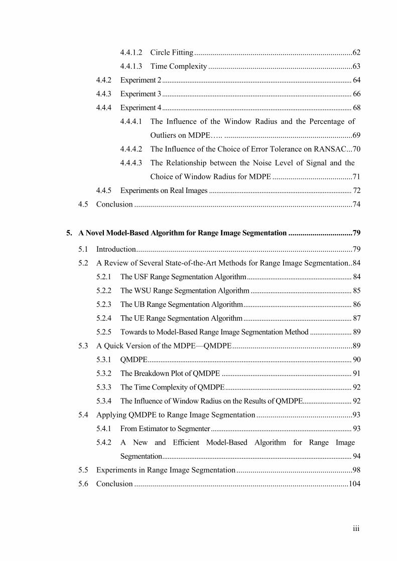
(a) (b)
Figure 1.2: Examples that many instances of a model can be simultaneously present in one
image: (a) there are many planar surfaces (i.e., instances of a planar model) in the range
image, (b) there are many cups (the rim of a cup can be roughly treated as a circle model)
in the color image.
Two frequently used robust techniques are the least median of squares (LMedS)
(Rousseeuw 1984) and the M-estimators (Huber 1981). One attractive feature of LMedS
and M-estimators is that they can tolerate up to half of the data points being arbitrarily bad.
In computer vision and image analysis, however, the data is often complex and several
instances of a model are simultaneously present, each accounting for a relatively small
percentage of the data points (see Figure 1.2). We call this case “data with multiple
structures”. Thus it will rarely happen that a given population achieves the critical size of
50% of the total population and, therefore, techniques that have been touted for their high
breakdown point (e.g., LMedS and other traditional robust methods from statistics) are no

4
longer reliable candidates, being limited to a 50% breakdown point. Only robust methods
designed with this special nature of the visual data in mind can achieve satisfactory results.
To design an efficient robust method for computer vision tasks, several characteristics that
are distinct from those (mostly) addressed by the statistical community must be taken into
account:
• Pseudo-outliers. In a given image, there are usually several populations of data
(i.e., multiple structures). Some parts correspond to one object in a scene and other
parts will correspond to other, rather unrelated, objects. When attempting to fit a
model to this data, one must consider the population belonging to the related object
as inliers and other populations as outliers - the term pseudo-outlier has been
coined (Stewart 1995). In computer vision tasks, it rarely happens that a given
population achieves the critical size of 50% of the total population and, therefore,
techniques that have been touted for their high breakdown point (e.g., the Least
Median of Squares) are no longer reliable candidates from this point of view.
• Large data sizes. Modern digital cameras exist with around 4 million pixels per
image. Image sequences, typically at up to 50 frames per second, contain many
images. Thus, computer vision researchers typically work with data sets in the tens
of thousands of elements, at least, and data sets in the 106 and 109 range are not
uncommon.
• Unknown sizes of populations and unknown location. Computer vision requires
fully automated analysis in, generally, rather unstructured environments. Thus, the
sizes and locations of the populations involved, will fluctuate greatly. Moreover,
there is no “human in the loop” to select regions of the image dominated by a single
population, or to adjust various thresholds. In contrast, statistical problems studied
in most other areas usually have a single dominant population plus some percentage
of outliers (typically mis-recordings - not the pseudo-outliers mentioned above).
Typically a human expert is there to assess the results (and, if necessary, crop the
data, adjust thresholds, try another technique etc.).

5
• Emphasis on fast calculation. Most tasks in computer vision must be performed
“on-the-fly”. Offline analysis that takes seconds, let alone minutes or hours, is
usually a luxury afforded by relatively few applications.
These rather peculiar circumstances have lead computer vision researchers to develop their
own techniques that perform in a robust fashion (perhaps “empirically robust” should be
used, as few have formal proved robust properties, though many trace their heritage to
techniques that do have such proved properties). These include ALKS (Lee, Meer et al.
1998), RESC (Yu, Bui et al. 1994), and MUSE (Miller and Stewart 1996). However, it has
to be admitted that a complete solution, addressing all of the above problems, is far from
being achieved. Indeed, none of the techniques, with present hardware limitations, are
really “real-time” when applied to the most demanding tasks. None have been proved to
reliably tolerate high percentages of outliers and, indeed, we have found with our
experiments that RESC and ALKS, although clearly better than the Least Median of
Squares, in this respect, are not always reliable. As we stated in the summary of this thesis,
one can improve upon these approaches by using extra information such as symmetry in
the data or the residual distribution.
This thesis addresses various problems in computer vision - specifically, robust model
fitting, range image segmentation, image motion estimation, fundamental matrix
calculation, and grey/color image segmentation. The major contributions of this thesis
come in following forms: (a) a new symmetry-based robust method; (b) several novel
highly robust methods with experimentally demonstrated advantages; (c) a novel highly
robust scale estimation technique; (d) several practical techniques applying the proposed
robust methods to solve “real” computer vision problems including range image
segmentation, optical flow calculation and fundamental matrix estimation; and (e) a couple
of algorithms for grey/color image segmentation. A more subtle contribution of this thesis
is that we, in looking at applying mean shift for histogram-based image segmentation,
noticed a quantizing effect that produces false peaks. We develop a theory to predict/avoid
false peaks and this theory is applicable in all situations where one quantizes feature space
(e.g., the residual space) before applying the mean shift. The methods/techniques
developed in this thesis can be beneficial to both the statistics and the computer vision
communities.

6
1.2 Thesis Outline
There are a wide range of topics covered in this thesis (model fitting; range image
segmentation; optical flow calculation; fundamental matrix estimation; grey/color image
segmentation). Thus, previous related work is reviewed or introduced when it is necessary.
In Chapter 2, several state-of-the-art robust techniques are reviewed. These robust
techniques include both those developed in the statistics field (such as M-Estimators,
Repeated Median, LMedS, and LTS) and those developed in the computer vision
community (such as Hough Transform, RANSAC, MINPRAN, MUSE, ALKS, and
RESC). Chapter 3 addresses the fragility of traditionally employed robust methods
(LMedS and LTS) when data involve clustered outliers, and analyses the reasons that cause
the fragility of these methods. Furthermore, the symmetry information in the data is
exploited and the concept of “Symmetry Distance” is introduced to model fitting. An
improved regression method — the LTSD is proposed. Chapter 4 takes advantage of
structure information in the pdf of the residuals in order to achieve higher robustness. By
employing nonparametric density estimation and density gradient techniques, and by
considering the distribution of probability density in the residual space, a novel and highly
robust estimator, MDPE, is proposed. Extensive experimental comparisons have been
carried out to show the advantages of MDPE compared with five frequently used robust
methods (LMedS, Hough Transform, RANSAC, ALKS, and RESC). Chapter 5 begins by
reviewing several state-of-the-art range image segmentation algorithms. Then a novel
model-based range image segmentation algorithm, derived from Quick-MDPE, is
proposed. Segmentation is a complicated task and it requires more than a simple
application of a robust estimator. Actually, our proposed algorithm tackles many subtle
issues and thereby provides a framework for those who want apply their robust estimators
to the task of range image segmentation. In Chapter 6, we introduce the problem of
optical flow calculation. Then, a modified QMDPE employing the variable bandwidth
technique (vbQMDPE) is applied to compute the optical flow. Because vbQMDPE has a
higher robustness to outliers than LMedS and LTS, the experiments on both synthetic and
real image sequences show very promising results.

7
Having a correct scale of inliers is important to the robust behaviour of a lot of estimators.
However, robust scale estimation is relatively neglected. Thus, Chapter 7 investigates the
behaviour of several state-of-the-art robust scale estimators for data with multiple
structures, and, by exploiting the information of shape distribution of residuals, proposes a
novel robust scale estimator: TSSE. Chapter 8 proposes, based on TSSE, a novel robust
estimator: ASSC and its variant ASRC. Experiments on model fitting, range image
segmentation and fundamental matrix estimation show that the proposed method is very
robust to data with discontinuities, multiple structures and outliers. In Chapter 9, we
directly apply the mean shift algorithm to grey/color image segmentation. In the process,
we identify an issue that affects the mean shift method when the data is heavily quantized.
We also solve a couple of practical problems: (i) we propose a quantitative relationship
between the appearance of false peaks and the value of the bandwidth h, which is
applicable for many methods employing the mean shift; (ii) we introduce the local
homogeneity into the mean shift algorithm. These result in two algorithms for grey/color
image segmentation. Finally, Chapter 10 summarizes what we have done and identifies
what remain to be challenging problems: suggesting future research work.

8
2. Model-Based Robust Methods: A Review
The history of seeking a robust method that can resist the effects of gross errors, i.e.
outliers, in fitting models is long. Since data contamination is usually unavoidable - (due to
such cases as faulty feature extraction, sensor noise and failure, segmentation errors,
multiple structures, etc.), there has recently been a general recognition that all algorithms
should be robust for accurate estimation. As pointed out by (Meer, Mintz et al. 1991), a
robust estimator should have followed properties:
• Good efficiency at the assumed noise distribution.
• Reliability in the presence of various types of noise.
• High breakdown point.
• Time complexity is not much greater than that of the Least Squares method.
Because linear models play a very important role in most modern robust methods and
many modern techniques are developed based on linear regression methods, this chapter
commences with reviewing a most frequently applied linear regression method: the LS
method. Several state-of-the-art robust techniques are then reviewed.
Chapter 2
Model-Based Robust Methods: A Review

9
2.1 The Least Squares (LS) Method
Linear regression analysis is an important tool in most applied science including computer
vision. The least squares method is one of the most famous linear regression methods and
it has been used in many scientific fields for a long time.
The classical linear model can be described in the following form [(Rousseeuw and Leroy
1987), pp.1]:
),...,1(...11 niexxy ipipii =+++= θθ ( 2.1)
where the variable yi is the response variable; and the variables xi1,…,xip are the
explanatory variables. The error term ei is usually assumed to be normally distributed with
mean zero and standard deviation σ.
We have n sets of observations on yi and (xi1,…,xip), for i=1,…n:
⋅⋅⋅⋅⋅⋅⋅⋅⋅⋅⋅⋅
⋅⋅⋅
=
npnn
p
xxy
xxy
XY
1
1111
),( ( 2.2)
where Y=( y1,…,yn )’ is a n-vector; X=( x(1),…, x(p) ) is a n-by-p matrix and x(i) = (xi1,…,xin)’
is a n-vector.
Equation ( 2.1) can be rewritten using matrix notation as follows:
Y=Xθ + e ( 2.3)
Using regression analysis, we can obtain regression coefficients )'ˆˆ(ˆ1 pθθθ ⋅⋅⋅= from the
observation data (Y, X). θ is the estimate of θ . Applying θ to the explanatory variables
(xi1,…,xip), we can obtain:

10
pipii xxy θθ ˆ...ˆˆ 11 ++= ( 2.4)
where iy is the estimated value of yi. Usually, this estimated value is not exactly the same
as the actually observed value. The difference between the estimated value iy and actually
observed value yi is the residual ri for the i'th set of observed data.
ri = yi - iy ( 2.5)
The ordinary least squares regression estimator can be written as follows:
∑=
=n
iir
1
2
ˆminargˆθ
θ ( 2.6)
Equation ( 2.6) is the well-known LS equation. From equation ( 2.6), we can see the least
squares estimator estimates the optimized θ by minimizing of the sum of the squared
residuals.
If we let:
S(θ ) =∑=
n
iir
1
2 ( 2.7)
Then, we have:
S(θ )= r’r = (Y-Xθ )’(Y-Xθ ) = Y’Y+θ ’X’X θ -2θ ’X’Y ( 2.8)
Differentiating S(θ ) w.r.t. θ , we obtain:
2X’Xθ -2X’Y = ˆ( ) 0ˆ
S θθ
∂ =∂
( 2.9)
From equation ( 2.9), we obtain the normal equation [(Rao and Toutenburg 1999), pp.24]:
X’Xθ = X’Y ( 2.10)
When X’X is not singular, the regression coefficients θ can be estimated by:
11
0 2 4 6 8 10 12-5
0
5
10
15
20
25
Clustered outliers
Pseudo-outliers
Leverage point
True Line
Inliers
Uniformly distributed outliers
θ = (X’X)-1X’Y ( 2.11)
The LS estimator is highly efficient and achieves optimum results under Gaussian
distributed noise. Although the LS method has the advantages of low computational cost
and high efficiency, it is extremely sensitive to outliers (gross errors or samples belonging
to another structure and distribution).
2.2 Outliers and Breakdown Point
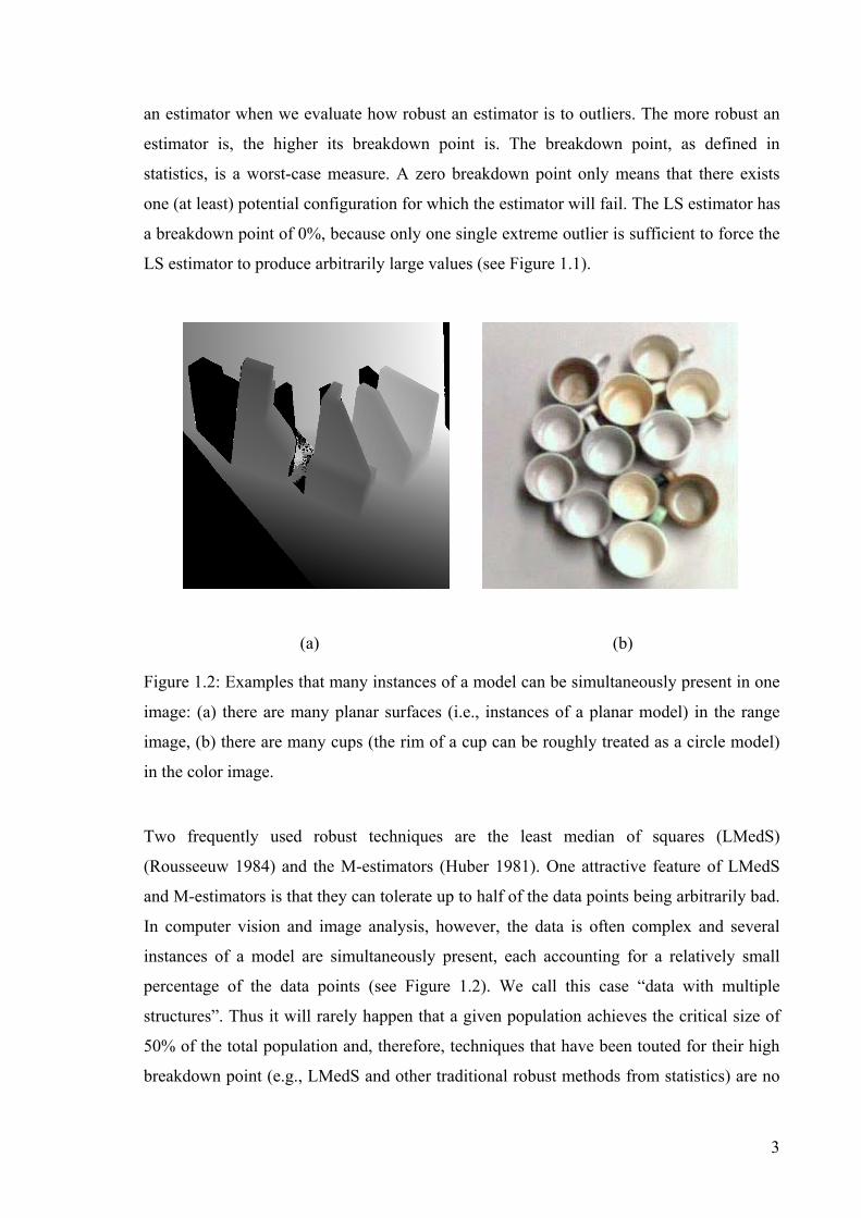
Figure 2.1: The types of outliers.
Outliers can be grossly defined as: “the data points that lie far from the majority of the
data”. Before we discuss the behavior of robust estimators, it is beneficial to investigate
the various types of outliers that one can encounter. Outliers frequently happen in the data
in computer vision tasks. Outliers could potentially lead to negative effects on the accuracy
of the results. Even more, outliers could seriously spoil the results of one method that is not
robust to outliers. Although a lot of new statistical techniques have been developed to
tolerate the effect of outliers within recent years, their advantages remain only when the
data involve certain types of outliers.

12
Loosely speaking, outliers can be classified into following four types:
• Leverage points — the outliers in explanatory variables.
• Clustered outliers — the outliers that are clustered.
• Randomly distributed outliers — the outliers that are randomly distributed.
• Pseudo outliers — the data points from structures that are extraneous to a particular
single parametric model fit, i.e., data that are inliers to one structure will be pseudo
outliers to another.
“Leverage point” means that the point is outlying relative to the explanatory variable xi, but
not relative to the response variable yi. Leverage points do not always lead to negative
results. When a leverage point lies close to a regression line, it is a “good leverage point”
(as shown in Figure 2.1) and can lead to a good effect on the results. However, the leverage
point is far away the regression line, it is a “bad leverage point” (i.e., outlier). Clustered
outliers often bring seriously negative effects to the results. It has been experimentally
shown that it is relatively hard to resist the effects of clustered outliers than those of
randomly distributed outliers (see chapter 3 and 4). Most theories are proposed assuming
that outliers are uniformly distributed. The theories that consider clustered outliers are
relatively less in number.
One characteristic to distinguish pseudo outliers from gross outliers and clustered outliers
is that pseudo outliers are coherent and structured. Pseudo outliers have structures while
gross outliers and clustered outliers do not have. Pseudo outliers often appear in the data
including multiple structures. Because multiple structures frequently happen in computer
vision tasks, studying the effects of pseudo outliers (multiple structures) has been popular
in computer vision community (Yu, Bui et al. 1994; Miller and Stewart 1996; Lee, Meer et
al. 1998; Bab-Hadiashar and Suter 1999).
To seek an estimator with high breakdown point is one of the most important topics among
the statistics and computer vision community. The breakdown point of an estimator may be
roughly defined as the smallest percentage of outlier contamination that can cause the
estimator to produce arbitrarily large values. Let Z be any sample of n data points (x1, y1),

13
…, (xn, yn), Z = {z1, …,zn} and zi = {xi, yi}. For m ≤ n, the finite-sample breakdown point of
a regression estimator T can be written as [(Rousseeuw and Leroy 1987), pp.10]:
∞==∈
)(sup;min),( **
*ZT
nmZT n
ZZn
m
ε ( 2.12)
Because one single outlier is sufficient to force the LS estimator to produce arbitrarily
large value, the LS estimator has a breakdown point of 0%.
In order to reduce the influence of outliers, many robust estimators with high breakdown
point have been developed during the past three decades. In the next sections, several
modern robust estimators, developed by both statistics and computer vision communities
will be reviewed.
2.3 Traditional Robust Estimators from Statistics
A lot of robust estimators have been developed within the statistics community and applied
to computer vision field. Among these robust estimators, the family of M-estimators is one
class of the most popular robust regression methods.
2.3.1 M-Estimators and GM-Estimators
The theory of M-estimators was firstly developed by Huber in 1964 and several years later.
It was successfully generalized as a robust regression method (Huber 1973; Huber 1981).
The essence of M-estimators is to replace the squared residuals 2ir in equation ( 2.6) by a
symmetric function ρ of the residuals:
ˆ 1
ˆ arg min ( )n
ii
rθ
θ ρ=
= ∑ ( 2.13)
where )( irρ is a robust loss function with a unique minimum when residual r is zero. The
purpose of introducing the loss function )( irρ is to reduce the effects of outliers.

14
Let the derivative of )( irρ be )( irψ , then differentiating∑=
n
iir
1)(ρ in equation 2.13, we obtain
0)ˆ/(1
=∑=
i
n
ii rr σψ ( 2.14)
where σ is the variance related to residuals. The solution of equation ( 2.14) could be
found using iterative minimization and various equation solving algorithms (Li 1985).
M-estimators can be classified into three types based on the influence function )( irψ
(Holland and Welsch 1977; Stewart 1997):
1. Monotone M-estimators. This type of M-estimators has nondecreasing,
bounded )(rψ functions [(Huber 1981), Chapter 7]. The loss functions can be
written as:
<−
≤=
rccrc
crrr
),2(21
,21
)(
2
ρ ( 2.15)
2. Hard Redescenders. This type of M-estimators forces )(rψ =0 when cr > (c is a
threshold). That is to say, a residual will lose its effects on the results when the
absolute of the residual is larger than c (Hampel, Rousseeuw et al. 1986a). The loss
functions )(rρ can be written as:
[ ]
≤−+
≤<−++−−
≤<−
≤
=
rcacba
crbacbcbcra
braara
arr
r
),(21
,)()/()(21
),2(21
,21
)(2
2
ρ ( 2.16)
3. Soft Redescenders. This type of M-estimators has not a finite rejection point c. The
type of M-estimators force )(rψ =0 when ∞→r .

15
)/1log()1(21)( 2 frfr ++=ρ ( 2.17)
Although the M-estimators are robust to outliers with respect to response variables, they
are not efficient in resisting the outliers with respect to explanatory variables (see equation
( 2.1)). Therefore, the generalized M-estimators (GM-estimators) were developed to reduce
the effects of outliers with respect to explanatory variables. GM-estimators used weight
function w to resist the influence of outliers with respect to explanatory variables.
Mallows (Mallows 1975) presented the following GM-estimators:
0)ˆ/()(1
=∑=
i
n
iii xrxw σψ ( 2.18)
Hill developed the following equation (Hill 1977):
0)ˆ)(/()(1
=∑=
i
n
iiii xxwrxw σψ ( 2.19)
Unfortunately, it has been proved that the breakdown point of GM-estimators is only
1/(1+p), where p is the dimension of explanatory variables (Maronna, Bustos et al. 1979).
That means when p=2, the highest breakdown point of GM-estimators is only 33.333%.
When p increases, the breakdown point will correspondingly diminish.
2.3.2 The Repeated Median (RM) Estimator
Before the development of the repeated median estimator, it was controversial whether it
was possible to find a robust estimator with a high breakdown point of 50%. In 1982,
Siegel proposed the repeated median (RM) estimator (Siegel 1982). The repeated median
estimator has an attractive characteristic in that it can obtain a 50% breakdown point.
The repeated median method can be summarized as follows: For any p observations, (xi1,
yi1),…,(xip, yip), let the solution parameter vector be denoted by '1
ˆ ˆ ˆ( ,..., )pθ θ θ= . The jth
coordinate of this vector is denoted by θ j (i1,…,ip). Then the repeated median estimator is
written as:

16
1 1i
ˆ (...( (p p
j i imed med medθ
−
= θ j (i1,…,ip)))…) ( 2.20)
The repeated median estimator is effective for problems with small p. However, the time
complexity of the repeated median estimator is O(nplogpn), which prevents the method
being useful in applications where p is even moderately large.
2.3.3 The Least Median of Squares (LMedS) Estimator
Rousseeuw proposed the least median of squares (LMedS) in 1984 (Rousseeuw 1984). The
LMedS method has the following assumptions:
• The signal to be estimated should occupy the majority of the data points, that is,
more than 50% data points should belong to the signal to be estimated (some
traditional methods such as RM, LTS, etc., also have the same assumption).
• The correct fit will correspond to the one with the least median of squared
residuals. This criterion is not always true when the data includes multiple
structures and clustered outliers, and when the variance of inliers is large (see
chapter 2 and 3).
The LMedS method is based on the simple idea of replacing the sum in least sum of
squares formulation by a median. LMedS finds the parameters to be estimated by
minimizing the median of squared residuals corresponding to the data points. The LMedS
estimate can be written as:
2
ˆminargˆ
iirmed
θθ = ( 2.21)
A drawback of the LMedS method is that no explicit formula exists for the solution of
equation ( 2.21) – the exact solution can only be determined by a search in the space of all
possible estimates. This space is very large. One can consider all estimates determined by
all possible p-tuples of data points. There are O(np) p-tuples and it takes O(nlogn) time to
find the median of the residuals of the whole data for each p-tuple. Thus it costs
O(np+1logn) for the LMedS method. The cost will thus increase very fast with n and p.
17
In practice, only an approximate LMedS, based upon random sampling, can be
implemented for any problem of a reasonable size – we generally refer to this approximate
version when we use the term LMedS (a convention adopted by most other authors as
well). In order to reduce the time complexity of the LMedS method to a feasible value, a
Monte Carlo type technique (described as follows) is usually employed.
A p-tuple is “clean” if it consists of p good observations without contamination by outliers.
One performs, m times, random selections of p-tuples, where one chooses m so that the
probability (P) that at least one of the m p-tuples is “clean” is almost 1. Let ε be the
fraction of outliers contained in the whole set of points. The probability P can be expressed
as follows:
P=1-(1-(1- ε)p)m ( 2.22)
Thus one can determine m for given values of ε, p and P by:
])-1(1log[
)1log(p
Pmε−
−= ( 2.23)
For example, if there are 50 percent of data contaminated by outliers, i.e. ε = 0.5, and if we
require P = 0.99; then, for circle fitting, p=3, we obtain m=35; and for ellipses fitting, if we
let p=5, then we obtain m=145.
The LMedS method has excellent global robustness and high breakdown point (i.e., 50%).
Over the last two decades, LMedS has been growing in popularity. For example, Kumar
and Hanson used the least median of squares to solve the pose estimation problem (Kumar
and Hanson 1989); Roth and Levine employed it for range image segmentation (Roth and
Levine 1990); Meer et. al. applied it for image structure analysis in the piecewise
polynomial field ; Zhang used the least median squares in conic fitting (Zhang 1997); and
Bab-Hadiashar and Suter employed it for optic flow calculation (Bab-Hadiashar and Suter
1998).
However, the relative efficiency of the LMedS method is poor when Gaussian noise is
present in the data. As Rousseeuw noted (Rousseeuw and Leroy 1987), the LMedS method
18
has a very low convergence rate: it is of order n-1/3, which is much lower than the
convergence rate of order n-1/2 of M-estimators. To compensate this deficiency, Rousseeuw
improved the LMedS method by carrying out a weighted least square procedure after the
initial LMedS fit. The weights are chosen based on the initial LMedS fit.
The preliminary scale (a detailed description sees chapter 7) estimate is given by:
251.4826(1 ) iiS med r
n p= +
− ( 2.24)
where ri is the residual of i'th sample.
The weight function Wi which will be assigned to the i'th data point is given by:
>
≤=
22
22
)5.2(0
)5.2(1
Sr
SrW
i
ii ( 2.25)
The data points corresponding to Wi=0 are likely to be outliers and will not be considered
in the further weighted least squares estimate. The data points having Wi=1 are inliers and
will be used for determining the final variance estimates σ .
Finally, σ is given by the weighted least squares
2ˆ
1
ˆ minn
i ii
W rθ
σ=
= ∑ ( 2.26)
There are different ways in which a method can be robust. The robustness we have been
discussing is global robustness. However, the LMedS method may be locally unstable
when fitting models to data. This means that a small change in the data can greatly alter the
output. This behaviour is not desirable in computer vision and has been noticed by Thomas
(Thomas and Simon 1992). In comparison, M-estimators have better local stability.

19
2.3.4 The Least Trimmed Squares (LTS) Estimator
The least trimmed squares (LTS) method was introduced by Rousseeuw to improve the
low efficiency of LMedS (Rousseeuw 1984; Rousseeuw and Leroy 1987). The LTS
estimator can be mathematically expressed as:
2:
ˆ 1
ˆ arg min ( )h
i ni
rθ
θ=
= ∑ ( 2.27)
where nnn rr :2
:12 )()( ≤⋅⋅⋅≤ are the ordered squared residuals, h is the trimming constant.
The LTS method uses h data points (out of n) to estimate the parameters. The coverage
value, h, may be set from n/2 to n. The aim of LTS estimator is to find the h-subset with
smallest least squares residuals and use the h-subset to estimate parameters of models. The
breakdown point of LTS is (n-h)/n. When h is set n/2, the LTS estimator has a high
breakdown value of 50%.
The advantages of LTS over LMedS are:
• It is less sensitive to local effects than LMedS, i.e. it has more local stability.
• LTS has better statistical efficiency than LMedS. It converges like n –1/2.
The implement of the LTS method also uses random sampling because the number of all
possible h-subsets ( hnC ) grows fast with n. There are two commonly employed ways to
generate a h-subset:
1. Directly generate a random h-subset from the n data points.
2. Firstly generate a random p-subset. If the rank of this p-subset is less than p,
randomly add data points until the rank is equal to p. Next, use this subset to
compute parameters jθ (j=1,…p) and residuals ri (i=1,…,n). Sort the residuals into
)(()(()1(( nrhrr πππ ≤⋅⋅⋅≤≤⋅⋅⋅≤ , and h-subset is set to: H:={ )(),...,1( hππ }.

20
Although the first way is easier than the second, the h-subset yielded by the first method
may contain a lot of outliers. Indeed, the chance of generating a “clean” h-subset by
method (1) tends to zero with increasing n. In contrast, it is easier to find a “clean” p-
subset without outliers. Therefore, method (2) can generate more (good) initial subset with
size h than method (1).
Like LMedS, the efficiency of LTS can be improved by adopting a weighted least squares
refinement as the last stage.
2.4 Robust Estimators Developed within the Computer Vision
Community
Although many robust estimators were developed in statistics during the past decades,
most of them can only tolerate 50% outliers. In computer vision tasks, it frequently
happens that outliers and pseudo-outliers occupy the absolute majority of the data.
Therefore, the requirement in these robust estimators that outliers occupy less than 50% of
all the data points is far from being satisfied for real tasks in computer vision. A good
robust estimator should be able to correctly find the fit when outliers occupy a higher
percentage of the data (more than 50%). Also, ideally, the estimator should be able to resist
the influence of all types of outliers (e.g., uniformly distributed outliers, clustered outliers
and pseudo-outliers).
Recently, many efforts have been made in computer community to find robust estimators,
which can tolerate more than 50% outliers. Among these high robust estimators, the
frequently used estimators are Hough Transform (Hough 1962), RANSAC (Fischler and
Rolles 1981), MINPRAN (Stewart 1995), MUSE (Miller and Stewart 1996), ALKS (Lee,
Meer et al. 1998), and RESC estimator (Yu, Bui et al. 1994). In the following sub-sections,
we will introduce these robust estimators. We commence with the explanation of
breakdown point as it is often interpreted by the computer vision community.
21
2.4.1 Breakdown Point in Computer Vision
In the statistical literature (Huber 1981; Rousseeuw and Leroy 1987), there are a number of
precise definitions of robustness and of robust properties: including the aforementioned
“breakdown point” (see section 2.2)– which is an attempt to characterize the tolerance of
an estimator to large percentages of outliers. Loosely put, such estimators should still
perform reliably even if up to 50% of the data do not belong to the model we seek to fit (in
statistics, these “outliers” are usually false recordings or other “wrong” data).
Estimators, such as the Least Median of Squares, that have a proven breakdown point of
0.5, have been much vaunted; particularly since this is generally viewed to be the best
achievable. It would be desirable to place all estimators on such a firm theoretical footing
by, amongst other things, defining and proving their “breakdown-point. However, in
practice, it is usually not possible to do so. Moreover, one can question whether the current
definitions of such notions are appropriate for the tasks at hand – in order to yield
mathematical tractability, they may be too narrow/restrictive. For example, does one care if
there is one single, unlikely if not impossible, configuration of data that will lead to the
breakdown of an estimator if all practical examples of data can be reliably tackled?
Moreover, as appealing as it is to quote theoretical results, it may mean little in practice.
Taking for example the Least Median of Squares estimator: the estimator is too costly to
implement and so everyone implements an approximate version of that estimator – no such
proofs exist (nor can they) assuring a precise breakdown point for such approximate
versions of the estimators. Not to mention the fact that there are data sets, having less than
50% outliers, where even the true Least Median of Squares will provably fail (for example
clustered outliers—see section 3.2); of course such configurations are carefully excluded
by the careful phrasing of the formal proofs of robustness. Yet clustered outliers, perhaps
unlikely in the mainstream statistical examples, are somewhat likely in computer vision
tasks when we consider the notion of pseudo-outliers (Stewart 1997) – data belonging to a
second “object” or “objects” within the image.
Several techniques (e.g., RANSAC, Hough transform) have experimentally proven
themselves as reliable workhorses (tolerating very high percentages of outliers – usually
much over 50%). We may say that these have an empirically determined very high
22
breakdown point, meaning that these are “unlikely” to breakdown and can usually tolerate
extremely high levels of outliers (much in excess of 50%).
Although the breakdown point in statistics is proved to be bounded by 0.5 [(Rousseeuw
and Leroy 1987), pp.125], the proof also shows that they require the robust estimator has a
unique solution (more technically, they require affine equivariance). When outliers
(including pseudo-outliers associated with multiple structures) occupy more than 50% of
the whole data, a robust method may return one of the multiple valued solutions (Yu, Bui
et al. 1994).
As Stewart said (Stewart 1999): the nature of computer vision problem alters the
performance requirements of the robust estimators in a number of ways. The optimum
breakdown point of 0.5 must be surpassed in some domains. A robust estimator with more
than 0.5 breakdown point is possible. That is, a robust estimator may have a higher than
0.5 breakdown point if we relax the single solution requirement, and permit the case of
multiple solutions to exist (Yu, Bui et al. 1994; Stewart 1995; Lee, Meer et al. 1998). This
can be done through the use of RANSAC or Hough Transform, or through adaptive
techniques based on scale estimates such as ALKS and MUSE, etc (Stewart 1999). Though
none of them have a theoretically proven breakdown point higher than 0.5, plausible
arguments, supported by experiments, suggest that they do in practice.
Thus, in this thesis, though we are motivated by the appealing notion of strictly provable
robustness in the form of high breakdown point, we follow a growing tradition of authors
(Yu, Bui et al. 1994; Stewart 1995; Lee, Meer et al. 1998) that present estimators, that have
empirically demonstrated robust qualities and are supported by plausible arguments, based
(as is, we might emphasize, the approximate Least Median of Squares technique used by
many statisticians and other scientists alike) on the similarity of the proposed technique to
estimators that do have provably high breakdown points.
2.4.2 Hough Transform (HT) Estimator
The Hough Transform was developed first to detect simple curves such as lines and circles
(Hough 1962). The basic Hough Transform is a voting technique. A typical

23
implementation of the technique is to count the number of data features that are mapped
into each cell in quantized parameter space. The Hough Transform has attracted a great
deal of attention, and many improvements have been made, like the generalized Hough
Transform, the probabilistic Hough Transform and the hierarchical Hough Transform
(Illingworth and Kittler 1988; Leavers 1993).
The Hough transform has been recognized as being a powerful tool in shape analysis,
model fitting, motion segmentation, which gives good results even in the presence of noise
and occlusion. Major shortcomings of the Hough Transform are excessive storage
requirements and computational complexity. Typically, the storage space and time
complexity required is about O(Np), where p is the dimension of parameter space and N is
the number that each parameter space is quantized into. Another problem of the Hough
Transform is its limited precision. Generally speaking, increasing the quantization number
of each parameter space will lead to a higher precision; however, this will also increase the
computational cost. Finally, though the Hough Transform can be successfully applied to
estimate multiple structures, one might have to solve many practical problems in multi-
modal parameter space. In effect, the hard problems have been deferred to the analysis of
parameter space. Though the Hough Transform tends to demonstrate robustness in the
presence of relatively high percentages of outliers, no formal proof of robustness (in terms
of breakdown point) seems to exist until very recently: we become aware of the work of
(Goldenshluger and Zeevi 2004), where the authors formalized the statistical properties of
the HT methodology and determined the breakdown point of the HT estimator.
2.4.3 Random Sample Consensus (RANSAC) Estimator
Fischler and Bolles (Fischler and Rolles 1981) provided a generate-and-test paradigm:
RANdom Sample Consensus (RANSAC). They used the minimum number of data points,
a p-subset (p is the dimension of parameter space), necessary to estimate the parameters of
the model. RANSAC, for its high robustness to outliers and ease to carry out, has been
widely employed in many computer vision tasks. The algorithm of RANSAC can be
described as follows:

24
1 Randomly choose a p-subset from the given n data points. This step has the similar
place to that used in LMedS, LTS, ALKS, etc. in that all of these estimators employ
a random sampling scheme.
2 Using this p-subset to determine the parameters of the model. Then, determine the
number of data points that are within some error tolerance of the model.
3 If the number is greater than a threshold, use the p-subset to determine a new model
by the least squares method and output the parameters of the model as results.
4 Otherwise, randomly choose a new p-subset and repeat step 1 and 2. If no consensus
with the threshold or more members has been found after running the
predetermined number of trails, either terminate the program or compute the
parameters of the model with the largest consensus set found.
From the procedure of RANSAC described above, we can see the RANSAC method need
three predetermined parameters:
• The error tolerance.
• The number of subsets to try.
• The threshold, which indicates whether or not the correct model has been
found.
If the predetermined parameters are correct, RANSAC is very robust to outliers and can
tolerate more than 50% outliers experimentally. However, if the predetermined parameters
or some of them (for example, the error tolerance) are wrong, the achievements of
RANSAC will be corrupted.
2.4.4 Minimize the Probability of Randomness (MINPRAN) Estimator
The MINPRAN estimator is one kind of robust estimator that has a higher than 50%
breakdown point (Stewart 1995). It can find a model in the data involving more than 50%

25
outliers without prior knowledge about error bounds. In contrast, the Hough Transform and
RANSAC techniques need a priori knowledge about the inlier bound of the correct fit.
The MINPRAN estimator is similar to the LMedS/LTS estimator but it outperforms the
LMedS/LTS estimator in the following ways:
• The MINPRAN estimator can find correct fit that involves less than 50% of the
data. The prerequisite of this achievement is that inliers need to be close to the
correct fit and outliers are randomly distributed.
• It does not “hallucinate” fits when there is not any model in the data. (The
MINPRAN estimator outputs nothing, not even a false fit, when there is no model
in the data). This is different from most other robust estimators such as M-
estimators, LMedS, LTS, etc.
• The LMedS/LTS estimators always use 50% of the data (for LMedS, see section
2.3.3) or h data points out of n data points (for LTS, see section 2.3.4) regardless of
the true percentage of the inliers in the whole data. MINPRAN, however, will
identify and use all inliers. Therefore, the MINPRAN estimator can yield more
accurate results than the LMedS and LTS estimators.
However, MINPRAN assumes that the outliers are randomly distributed within a certain
range. This makes MINPRAN less effective in extracting multiple structures and clustered
outliers. At the same time, it occasionally finds the fits that actually bridge small
magnitude discontinuities.
2.4.5 Minimum Unbiased Scale Estimator (MUSE) and Adaptive Least kth Order
Squares (ALKS) Estimator
Miller and Stewart proposed the minimum unbiased scale estimator (MUSE) in 1996
(Miller and Stewart 1996). MUSE was designed to extract surfaces that contained less than
50% of the data without a priori knowledge about the percentage of the inliers and to detect
the small-scale discontinuities in the data. MUSE is based on the LMedS method, but it
improves LMedS and can accurately estimate fits when the data contain multiple surfaces.

26
MUSE randomly selects p-subsets and then estimates fits based on these p-subsets. It then
calculates the unbiased estimate of the scale for each fit’s k smallest residuals, where k is
set to all possible values and satisfies 1 ≤ k ≤ N-p; Then the smallest scale estimate over all
possible k is chosen as the representative value of the hypothesized fits. Finally, the fit
from the p-subset with the smallest scale estimate is chosen as the optimum fit. The scale
estimate can be written as:
][ :
:
Nk
Nkk uE
rs = ( 2.28)
where rk:N is the kth ordered absolute residual, and E[uk:N] can be approximated by:
)2/)1
1((][ 1: +
+Φ≈ −
NkuE Nk ( 2.29)
where [.]1−Φ is the argument of the normal cumulative density distribution.
Because the scale estimate is biased, a correction is taken to eliminate the bias by
normalizing the sk. The unbiased minimum scale estimate can be written as:
kkk
kk
skvE
s
]minarg'|[min
min
' ==ϕ ( 2.30)
where vk is the kth scale estimate.
Because it takes O(n3) time to calculate E[minv|k], these are pre-calculated and stored in a
table, which will be used when MUSE is carried out.
Inspired by MUSE, Lee and Meer provided the adaptive least kth order squares (ALKS)
estimator (Lee, Meer et al. 1998). ALKS is based on the least kth order squares (LKS)
[(Rousseeuw and Leroy 1987), pp.124]. LKS procedure is similar to those of the LMedS
estimator. The difference between LKS and LMedS is in that LKS uses k data points out of
n data points (p<k<n), while LMedS uses half of the n data points. The breakdown point
of LKS is min(k/n, 1-k/n). Because it is impossible for a robust estimator using a one-step
procedure to have a breakdown point exceeding 50%, ALKS uses multi-step procedure (in

27
each step, ALKS employs LKS with different k value) and recovers the fit to the relative
majority of the data without any priori knowledge about the scale of inliers.
ALKS uses k data points out of n data points. The robust estimate of the noise scale can be
written as:
]2
/1[
ˆˆ
1
min
nkd
s kk +Φ
=−
( 2.31)
where dkmin is the half-width of the shortest window containing k residuals.
This estimate of noise scale is only valid when the k is not very large or very small. After
ks is estimated, the variance of the normalized error is computed as follows:
2
21
2,
2
2
1
,2
ˆˆ
ˆ1
ˆ1
k
k
k
q
iki
k
q
i k
ki
kk spq
r
ssr
pq
k
k σ=
−=
−
=Ε∑
∑ =
=
( 2.32)
ALKS assumes that the optimum value of k should yield the least 2kΕ .
In order to estimate the correct k, a random sampling technique, similar to that used in
LMedS and RANSAC, is also employed in ALKS. The ALKS method can deal with data
with multiple structures, but it cannot resist the influence of the extreme outliers.
The authors of MUSE and those of ALKS consider robust scale estimate in their methods
and they both can obtain a greater than 50% breakdown point. MUSE and ALKS can
perform better than LMedS and M-estimators at small-scale discontinuities. However,
MUSE needs a lookup table for the scale estimate correction; ALKS is limited in its ability
to handle extreme outliers. Another problem we found in ALKS is its instability under a
small percentage of outliers.

28
2.4.6 Residual Consensus (RESC) Estimator
Yu et al. presented a highly robust estimator for range image segmentation and
reconstruction (Yu, Bui et al. 1994). Because this method considers residual consensus, it
is called RESC. RESC greatly improves the robustness of an estimator to outliers.
Although there have been some estimators appearing in the literature (such as Hough
Transform and RANSAC) that might tolerate more than 50% outliers, RESC claims that it
can reach a high breakdown point which can tolerate more than 80% outliers. This
attractive characteristic of the RESC method is achieved by using a histogram compression
approach for residual consensus.
The basic idea of the RESC method is that if a model is correctly fitted, the residuals of
inliers should be small and, at the same time, the histogram of the residuals should
concentrate within a small range in the lower part of the histogram. In the RESC method, a
histogram compression technique plays an important role in residual consensus. The
histogram compression technique works as follows:
1. Estimate the original histogram of residuals with as many histogram columns (says
2000) as possible. The estimated histogram of residuals will be used for
compression in the following steps.
2. Decide the column width of the compressed histogram. The width is chosen where
the first column of the compressed histogram can contain p percent of all data
points. The value of p is experimentally chosen as 12. Then the number v of
consecutive columns in the original histogram can be easily determined (these
consecutive columns of the original histogram will contain p percent of the data
points).
3. Then every v columns in the original histogram is compressed into one column in
the compressed histogram.
From the details of the histogram compression, we can see that the column width of the
compressed histogram depends on the noise level, which will change for different types of
data. Instead of using only residual information in its objective function, the RESC method

29
considers two factors in its objective function: the number of inliers and the residuals of
the inliers.
The RESC method defined its objective function as:
βαβψ ih
vm
i i /11∑ =
= ( 2.33)
where i is the ith column in the compressed histogram; hi is the number of points in the ith
column. α and β are coefficients which determine the relative importance of hi and i. They
are empirically determined as: α =1.3; and β =1.0. ψ is also called histogram power.
The procedure of the RESC method is as follows:
1. Randomly choose k sets of p-subset from the whole data points. A modified genetic
algorithm is used by the RESC method to improve the speed.
2. Calculate the residuals and compress the histogram of the residuals.
3. Select a p-subset from the k sets whose histogram power is the highest.
4. Determine the standard variance of the residuals.
5. Label the points of this primitive and remove them from the whole data points.
6. Remove the outliers in the labelled region.
7. Repeat step 1-6 until all signals are extracted.
The RESC method is very robust to noise. It finds the parameters by the p-subset
corresponding to the maximum of the histogram power. However, a disadvantage of the
RESC method is that it needs user to tune many parameters for the optimal performance.

30
2.5 Conclusion
In this chapter, we have reviewed several traditional and state-of-the-art robust estimators,
with their advantages and disadvantages. In the following chapters, we will, by using the
extra information inside the residuals, proposed novel efficient robust methods and apply
them to computer vision tasks.

31
3. Using Symmetry in Robust Model Fitting
3.1 Introduction
The pattern recognition and computer vision communities often employ robust methods for
model fitting (Fischler and Rolles 1981; Rousseeuw 1984; Rousseeuw and Leroy 1987;
Zhang 1997; Danuser and Stricker 1998; Stewart 1999). It is common to employ
“regression analysis” to undertake such tasks (Rousseeuw and Leroy, 1987). In particular,
high breakdown-point methods such as Least Median of Squares (LMedS) and Least
Trimmed Squares (LTS) have often been used in situations where the data are
contaminated with outliers. LMedS and LTS are based on the idea that the correct fit will
correspond to the one with the least median of residuals (for LMedS), or the least sum of
trimmed squared residuals (for LTS). The essence of the argument claiming a high
breakdown point for the LMedS is that if the uncontaminated data are in the majority, then
the median of the squared residuals should be unaffected by the outliers, and thus the
median squared residual should be a reliable measure of the quality of the fit. Likewise,
since the LTS method relies only on (the sum of squares of) the h smallest residuals, for
some choice of the parameter h, it is thought that this should be robust to contamination so
long as h data points, at least, belong to the true fit.
1.1.2. Chapter 3
Using Symmetry in Robust Model Fitting

32
However, though the breakdown point of these methods can be as high as 50% (they can
be robust to up to 50% contamination), they can break down at unexpectedly lower
percentages when the outliers are clustered. Due to the affects of clustered outliers, the
correct fit may not correspond to the fit with the least median of squared residual (for
LMedS) or the least trimmed squared residuals (for LTS). It is worth mentioning that this
phenomenon is not limited to LMedS, and LTS. It also happens to most other robust
estimators such as random sample consensus—RANSAC (Fischler and Rolles 1981),
residual consensus estimator—RESC (Yu, Bui et al. 1994), adaptive least k squares
estimator—ALKS (Lee, Meer et al. 1998), etc. The mechanism of the breakdown in these
robust estimators is similar to that of the LMedS and LTS (see chapter 4).
This illustrates a general principle: most robust methods only depend upon a single
statistical property (the sum of the trimmed squared residuals or the median of the squared
residuals, for example) and these methods ignore many other properties that the data, or the
residuals to the fit, should have. The key to salvaging the robustness of LMedS and LTS
(and some other robust estimators), even in the presence of clustered outliers, can be that
one looks beyond the standard definition of the robust methods to incorporate other
measures and statistics into the formulation. In this chapter, we restrict ourselves to one
such property – symmetry.
Symmetry is very common and important in our world. When we will fit circles, ellipses,
or any symmetric object, one of the most basic features in the model is symmetry. In our
method, we introduce the concept of symmetry distance (SD) and thereby we propose, by
taking advantage of the symmetry information in the visual data, an improved method,
called the least trimmed symmetry distance (LTSD). The symmetry we employ, in this
context, is that of symmetry about a central point (central with respect to the shape of
interest). The LTSD method is influenced not only by the sizes of the residuals of data
points, but also by the symmetry of the data points and has applications where one is trying
to fit a symmetric model (e.g. circle and ellipses). Experimental results show that the
LTSD approach gives better results than the LMedS method and the LTS method in
situations where a large percentage of clustered outliers and large standard variance in
inliers are encountered.

33
The main contributions of this chapter are as follows:
1. We illustrate situations where LMedS and LTS to fail to correctly fit the data in the
presence of clustered outliers, and analyze the reasons that cause the breakdown of
these two methods. This provides an important cautionary note when employing
these two robust estimators in situations where the outliers are clustered.
2. We introduce the concept of symmetry distance (SD) into model fitting. The
concept of SD in computer vision is not novel. However it is a novel concept in the
field of model fitting. Based on Su et al.’s point symmetry distance (Su and Chou
2001), we propose a novel symmetry distance and apply it to model fitting.
3. We experimentally show that the proposed method works better than LMedS and
LTS under a large percentage of clustered outliers for both simulated and real data.
This chapter is organized as follows: in section 3.2, the factors that cause both LMedS and
LTS to fail to fit a model under a large percentage of clustered outliers are explored. In
section 3.3, a novel symmetry distance measure is given and our proposed method is
developed in section 3.4. Experiments demonstrating the utility of the approach (for circle
fitting and ellipses fitting) are given in section 3.5. Finally, some conclusions and future
work are summarized in section 3.6.
3.2 Dilemma of the LMedS and the LTS in the Presence of
Clustered Outliers
The LMedS method and the LTS method are based on the idea that the correct fit is
determined by a simple statistic: the least median of the squared residuals (for LMedS), or
by the least sum of trimmed squared residuals (for LTS); and that such a statistic is not
influenced by the outliers.
Consider the contaminated distribution defined as follows (Haralick 1986; Hampel,
Rousseeuw et al. 1986b):

34
F=(1- ε)F0+ εH ( 3.1)
where F0 is an inlier distribution, and H is an outlier distribution.
Figure 3.1: An example where LMedS and LTS (h is set to 0.5n) fail to fit a circle yet there
are under 44.5% outliers – though, of course, the outliers are clustered.
Equation ( 3.1) is also called the gross error model. When the standard variance of F0 is
small (<<1) and that of H is large or H is uniform distributed, the assumptions leading to
the robustness of LMedS or LTS, are true. However, when F0 is “scattered”, i.e. the
standard variance of F0 is big, and H is clustered distributed with high density, the
assumption is not always true.
Let us investigate an example. In Figure 3.1, F0 (bivariate normal with unit variance)
including 100 data points were generated by adding the noise to samples of a circle with
radius 10.0 and center at (0.0, 0.0). Then 80 clustered outliers were added, possessing a
spherical bivariate normal distribution with one unit standard variance and mean (20.0,
6.0). As Figure 3.1 shows, both LMedS and LTS failed to fit the circle: LMS returned the
result with a radius equal to 7.4239 and the center was located at (13.1294, 8.6289). The
results obtained by LTS were: the radius was 19.3069 and the center was at (1.1445,
10.1470).
-20 -15 -10 -5 0 5 10 15 20 25 -10
-5
0
5
10
15
20
25
By LMS
By LTS
Clustered outliers

35
It is important to point out that the failure is inherent, and not simply an artifact of our
implementation. Let us check the median of the residuals (for LMedS) and the sum of
trimmed squared residuals (for LTS) and we will understand why LMedS and LTS failed
to fit to the circle. The median of residuals of the perfect fit is 5.7928. However the median
of residuals of final result by the LMedS method is 5.1479.
Figure 3.2: LMedS searches for the “best” fit with the least median of residuals.
Figure 3.2 shows the time evolution of the parameters: median of residuals (top left),
centre of the fitted circle (x coordinate and y coordinate in the top right and bottom left,
respectively), and the radius of the fitted circle (bottom right) as LMedS searches for the
“best” fit with the least median of residuals. (Note: the iterations pass by the correct fit
(pointed out by arrows) proceeding to fits with even lower median of residuals.) In fact,
during the searching procedure, the LMedS estimator consistently minimizes the median of
the residuals, starting with initial fits that have a larger median residual than the true fit, but
successively finding fits with lower median residuals – proceeding to even lower median
residuals than that possessed by the true fit.
The reason that LTS failed is similar. LTS finds the fit with smallest trimmed squared
residuals. The value of the least sum of trimmed squared residuals obtained is 32.6378.
However, the same statistic for the “true fit” is 58.6688. Clearly, LTS has “correctly”, by
0 5 105
5.5
6
6.5 Median Function
0 5 10 0
5
10
15 Xc
0 5 100
2
4
6
8
10 YC
0 5 10 6
8
10
12
14
16Radius

36
0 5 10 15 20 25 30 35 40 45 50
8
10
12
14
16
18
20
Percentage of clustered outliers
Est
imat
ed ra
dius
by
LMS
std=0.4 std=0.7 std=1.0 std=1.3 std=1.6
Percentage of clustered outliers
Estim
ated
radi
us b
y LT
S
0 5 10 15 20 25 30 35 40 45 50
8
10
12
14
16
18
20
22
24 std=0.4std=0.7std=1.0std=1.3std=1.6
-15 -10 -5 0 5 10 15 20 25
-10
-5
0
5
10
15
20
its criterion, obtained a “better” fit (but in fact, the wrong one). The problem is not with the
implementation but with the criterion
(a)
(b) (c)
Figure 3.3: Breakdown Plot: (a) One case of the distribution of data; The results of LMedS
(b) and LTS (c) in circle fitting will be affected by the standard variance of inliers and
percentages of clustered outliers.
Now, let us consider another example showing that the results of the LMedS and the LTS
are affected by the standard variance of the inliers. We generated a circle with radius 10.0
and center at (0.0, 0.0). In addition, clustered outliers were added to the circle with mean
(20.0, 6.0) and unit standard variance. In total, 100 data points were generated. At first, we
assigned 100 data to the circle without any outliers. Then we repeatedly moved two points
from the circle to the clustered outliers until 50 data were left in the circle. Thus, the
percentage of outliers changed from 0 to 50%. In addition, for each percentage of clustered
outliers, we varied the standard variance of the inliers from 0.4 to 1.6 with a step size of

37
0.3. Figure 3.3 (a) illustrates one example of the distribution of the data, with 38%
clustered outliers and the standard variance of inliers 1.3.
From Figure 3.3 (b), we can see that when the standard variance of inliers is no more than
1.0, LMedS can give the right results under a high percentage of outliers (more than 44%).
However, when the standard variance of inliers is more than 1.0, LMedS does not give the
right result even when the percentage of outliers is less then 40%. From Figure 3.3 (c), we
can see when the standard variance of inliers is 0.4, the LTS estimator can correctly give
the results even under 50% clustered outliers; while when the standard variance of inliers is
1.6, LTS does not give the right results even when only 30 percent of the data are outliers.
From the discussion above, we now see several conditions under which LMedS and LTS
failed to be robust. A crucial point is: these methods measure only one single statistic: the
least median of residuals or the least sum of trimmed squared of residuals, omitting other
characteristics of the data. If we look at the failures, we can see that the results lost the
most basic and common feature of the inliers with respect to the fitted circle—symmetry.
In the next section, we will introduce the concept of symmetry distance into robust
regression methods and propose an improved method, called the Least Trimmed Symmetry
Distance (LTSD), by which the better performance is acquired even when data include
clustered outliers.
3.3 The Symmetry Distance
Symmetry is considered a pre-attentive feature that enhances recognition and
reconstruction of shapes and objects (Attneave 1995). Symmetry exists almost everywhere
around us. A square, a cube, a sphere, and a lot of geometric patterns show symmetry.
Architecture usually displays symmetry. Symmetry is also an important parameter in
physical and chemical processes and is an important criterion in medical diagnosis. Even
we human beings show symmetry, (for instance, our faces and bodies are roughly
symmetrical between right and left). One of the most basic features in the shapes of models
we often fit/impose on our data, e.g. circles and ellipsis, is the symmetry of the model.

38
Symmetric data should suggest symmetric models and data that is symmetrically
distributed should be preferred as the inlier data (as opposed to the outliers). For decades,
symmetry has widely been studied in computer vision community. For example,
considerable efforts have been focused on the detection of symmetry in images in regard to
mirror symmetries (Marola 1989; Nalwa 1989) and in regard to circular symmetries (Bigun
1988; Reisfeld, Wolfson et al. 1992); Kirby etc. used the symmetric features of images for
image compression (Kirby and Sirovich 1990); Zabrodsky treated symmetry as a
continuous feature and applied it in finding the orientation of symmetric objects
(Zabrodsky, Peleg et al. 1995); Skewed symmetries in 3D structures have been extensively
studied (Oh, Asada et al. 1988; Ponce 1990; Gross and Boult 1994). Symmetry has also
been treated as a feature in cluster analysis (Su and Chou 2001). More detailed definitions
of symmetry can be found in (Zabrodsky 1993). We demonstrate here that symmetry can
also be used as a feature to enhance the performance of robust estimators when fitting
models with symmetric structure.
3.3.1 Definition of Symmetry
There are many kinds of symmetry in existence in the world. Generally speaking,
symmetry can be classified into the following four basic types, which are shown in Figure
3.4, (Zabrodsky 1993; Zabrodsky, Peleg et al. 1995):
1. Mirror-symmetry: if an object is invariant under a reflection about a line (for 2D) or
a plane (for 3D).
2. Cn-symmetry: if an object is invariant under rotation of nπ2 radians about its center
(for 2D) or a line passing through its center (for 3D).
3. Dn-symmetry: if an object has both mirror-symmetry and Cn-symmetry.
4. Circular-symmetry: if an object has ∞C -symmetry.

39
(a) (b)
(c) (d)
Figure 3.4: Four kinds of symmetries: (a) mirror-symmetry; (b) C4-symmetry; (c) D4-
symmetry; (d) circular symmetry.
3.3.2 The Symmetry Distance
The exact mathematical definition of symmetry (Weyl 1952; Miller 1972) is insufficient to
describe and quantify symmetry found both in the natural world and in the visual world.
Su and Chou proposed a symmetry distance measure based on the concept of “point
symmetry” (Su and Chou 2001). Given n points xi, i =1,…n and a reference vector C (e.g.
the centroid of the data), the point symmetry distance between a point xj and C is defined
as follows:
CxCx
CxCxCxd
ij
ij
jiandNijs −+−
−+−=
≠=
)()(min),(
,...1
( 3.2)
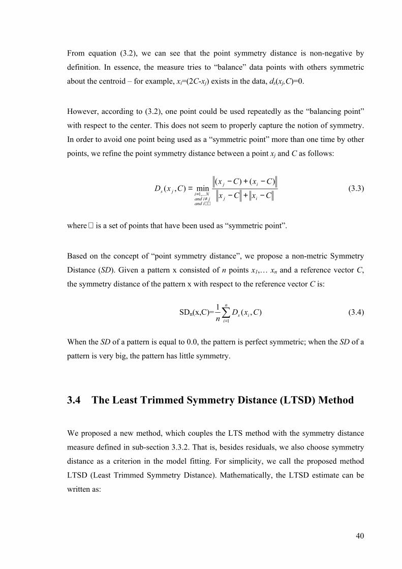
40
From equation ( 3.2), we can see that the point symmetry distance is non-negative by
definition. In essence, the measure tries to “balance” data points with others symmetric
about the centroid – for example, xi=(2C-xj) exists in the data, ds(xj,C)=0.
However, according to ( 3.2), one point could be used repeatedly as the “balancing point”
with respect to the center. This does not seem to properly capture the notion of symmetry.
In order to avoid one point being used as a “symmetric point” more than one time by other
points, we refine the point symmetry distance between a point xj and C as follows:
CxCx
CxCxCxD
ij
ij
iandjiand
Nijs −+−
−+−=
ℜ∉≠
=
)()(min),(
,...1 ( 3.3)
where ℜ is a set of points that have been used as “symmetric point”.
Based on the concept of “point symmetry distance”, we propose a non-metric Symmetry
Distance (SD). Given a pattern x consisted of n points x1,… xn and a reference vector C,
the symmetry distance of the pattern x with respect to the reference vector C is:
SDn(x,C)= ∑=
n
iis CxD
n 1
),(1 ( 3.4)
When the SD of a pattern is equal to 0.0, the pattern is perfect symmetric; when the SD of a
pattern is very big, the pattern has little symmetry.
3.4 The Least Trimmed Symmetry Distance (LTSD) Method
We proposed a new method, which couples the LTS method with the symmetry distance
measure defined in sub-section 3.3.2. That is, besides residuals, we also choose symmetry
distance as a criterion in the model fitting. For simplicity, we call the proposed method
LTSD (Least Trimmed Symmetry Distance). Mathematically, the LTSD estimate can be
written as:

41
),(minargˆ,
CxSDhCθθ = ( 3.5)
Only h data points with the smallest sorted residuals are used to calculate the symmetry
distance. The estimated parameters correspond to the least symmetry distance.
The specific details of the proposed method are given as follows:
1. Set repeat times (RT) according to equation ( 2.23). Initialise h with [(n+p+1)/2] ≤ h
≤ n. If we want LTSD to have a high breakdown point, say 50%, we can set
h=(n+p+1)/2.
2. Randomly choose p-subsets, and extend to h-subset H1 by the method (2) in sub-
section 2.3.4.
3. Compute 1θ by LS method based on H1. Compute symmetry distance SD1 based on
1θ and H1 using equation ( 3.4) in sub-section 3.3.2 and using the centre of the fit
(circle or ellipse) as the reference vector C. Decrement RT and if RT is smaller than
0, go to step 4, otherwise, go to step 2. We calculate the parameters θ based on h-
subset instead of p-subset in order to improve the statistical efficiency.
4. Finally, output θ with the lowest SD.
3.5 Experimental Results
In this section, we will show several examples using the proposed method to fit a model
with symmetrical structures. Circle fitting and ellipses fitting have been very popular
topics in the computer vision field. One of the obvious characteristics of circles and
ellipses is that they are symmetric. We first present an example of circle fitting; then we
present a relatively more complicated example of ellipse fitting. The results are compared
with those of the LMedS method and the LTS method.

42
3.5.1 Circle Fitting
In Figure 3.5, about 45 percent clustered outliers were added to the original circle data.
Since LMedS and LTS only rely on the residuals of the data points, their results were
affected by the standard variance of the inliers and percentages of the clustered outliers.
Therefore, they failed to fit the circle under a high percentage of clustered outliers (see
Figure 3.1). However, because the LTSD method considers the symmetry of the object,
this enables LTSD find the right model (see Figure 3.5): the true centre and radius of the
circle are respectively (0.0,0.0) and 10.0; by the LTSD method, we obtained centre (-0.23,
0.01) and radius10.06.
Figure 3.5: Using the symmetry of the circle, the LTSD method found the approximately
right results under 44.5% clustered outliers.
Another example showing the advantages of the proposed method is given in Figure 3.6 (a)
(corresponding to Figure 3.3 (a)). From Figure 3.6 (a), we can see that when the outliers
are clustered, the LMedS and LTS broke down under very low percentages of outliers, in
this case, they both broke down under 38% outliers! In comparison to the LMedS and LTS
methods, the proposed method gives the most accurate results. The proposed method is
affected less by the standard variance of the inliers and the percentages of the clustered
outliers. Figure 3.6 (b) shows that the radius found by the LTSD method in circle fitting
(true radius is 10.0) changed less under different standard variance of the inliers and
percentages of clustered outliers. In comparison to Figure 3.3 (b) and (c), the fluctuation of
-10 -5 0 5 10 15 20
-10
-5
0
5
10
Inliers Clustered outliersTrue circle Circle by LTSD
True circle
By LTSD
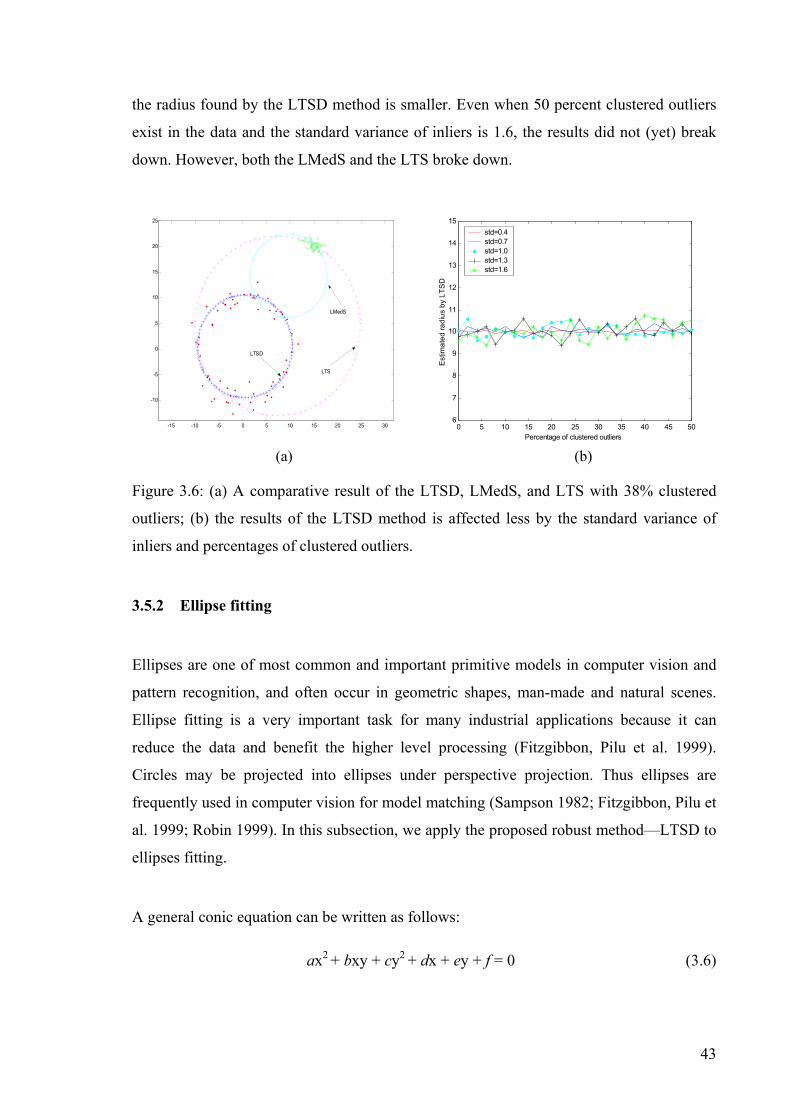
43
0 5 10 15 20 25 30 35 40 45 506
7
8
9
10
11
12
13
14
15
Percentage of clustered outliers E
stim
ated
radi
us b
y LT
SD
std=0.4std=0.7std=1.0std=1.3std=1.6
-15 -10 -5 0 5 10 15 20 25 30
-10
-5
0
5
10
15
20
25
LMedS
LTS
LTSD
the radius found by the LTSD method is smaller. Even when 50 percent clustered outliers
exist in the data and the standard variance of inliers is 1.6, the results did not (yet) break
down. However, both the LMedS and the LTS broke down.
(a) (b)
Figure 3.6: (a) A comparative result of the LTSD, LMedS, and LTS with 38% clustered
outliers; (b) the results of the LTSD method is affected less by the standard variance of
inliers and percentages of clustered outliers.
3.5.2 Ellipse fitting
Ellipses are one of most common and important primitive models in computer vision and
pattern recognition, and often occur in geometric shapes, man-made and natural scenes.
Ellipse fitting is a very important task for many industrial applications because it can
reduce the data and benefit the higher level processing (Fitzgibbon, Pilu et al. 1999).
Circles may be projected into ellipses under perspective projection. Thus ellipses are
frequently used in computer vision for model matching (Sampson 1982; Fitzgibbon, Pilu et
al. 1999; Robin 1999). In this subsection, we apply the proposed robust method—LTSD to
ellipses fitting.
A general conic equation can be written as follows:
ax2 + bxy + cy2 + dx + ey + f = 0 ( 3.6)

44
where (a,b,c,d,e,f) are the parameters needed to find from the given data. When b2 < 4ac,
the equation above corresponds to ellipses.
The ellipse can also be represented by its more intuitive geometric parameters:
1)cossincossin(
)sincossincos(
2
2
2
2
=−++−+
−−+
Byxyx
Ayxyx
cc
cc
θθθθ
θθθθ
( 3.7)
where (xc, yc) is the center of the ellipse, A and B are the major and minor axes, and θ is the
orientation of the ellipse.
The relation between (a,b,c,d,e,f) and (xc, yc, A, B, θ) can be written as (Robin 1999):
(5.3)
It is convenient to find (a,b,c,d,e,f) first by the given data and then convert to (xc, yc, A, B,
θ).
As illustrated in Figure 3.7 and Table 3.1, 200 data were generated with 40% clustered
outliers. The outliers were compacted within a region of radius 5 and center at (20.0, 5.0).
The ellipse had a standard variance 0.8, major axis 10.0, minor axis 8.0, center (0.0,0.0),
and orientation to horizon direction θ is 0.0 degree. The results of LTS and LMedS were
seriously affected by the clustered outliers. However, the LTSD method worked well.
−=
−+±+
−=
−−=
−−=
−
cab
fcabfca
fBA
bacaebdy
baccdbex
c
c
1
22
2
2
tan21
)(
22},{
42
42
θ

45
-10 -5 0 5 10 15 20 25-10
-5
0
5
10
15
20InliersClustered outliersBy LTSDBy LTSBy LMedS
Figure 3.7: Comparison of the results obtained by the LTSD method, LTS and LMedS in
ellipse fitting under 40% clustered outliers.
Next, we will apply the LTSD method to real images.
3.5.3 Experiments with Real Images
The first example is to fit an ellipse in an image of a mouse pad, shown in Figure 3.8. The
edge image was obtained by using Canny operator with threshold 0.07. In total, 310 data
points were in the edge image (Figure 3.8 (b)). The clustered outliers, due to the flower,
occupy 50% of the data. Three methods (the LTSD, LTS and LMedS) were applied to
detect the mouse pad edge. As shown in Figure 3.8 (c), both LTSD and LTS correctly
found the edge of the mouse pad. However, LMedS fails to detect the edge of the mouse
xc yc Major axis Minor axis θ (deg)
True value 0.0 0.0 10.0 8.0 0.0
The LTSD method -0.125 -0.145 9.760 7.810 6.355
The LTS method 19.786 5.162 3.328 3.035 34.129
The LMedS method 9.560 5.208 11.757 3.679 -3.307
Table 3.1: Comparison of the estimated parameters by the LTSD, LTS, and
LMedS methods in ellipses fitting under 40% clustered outliers.
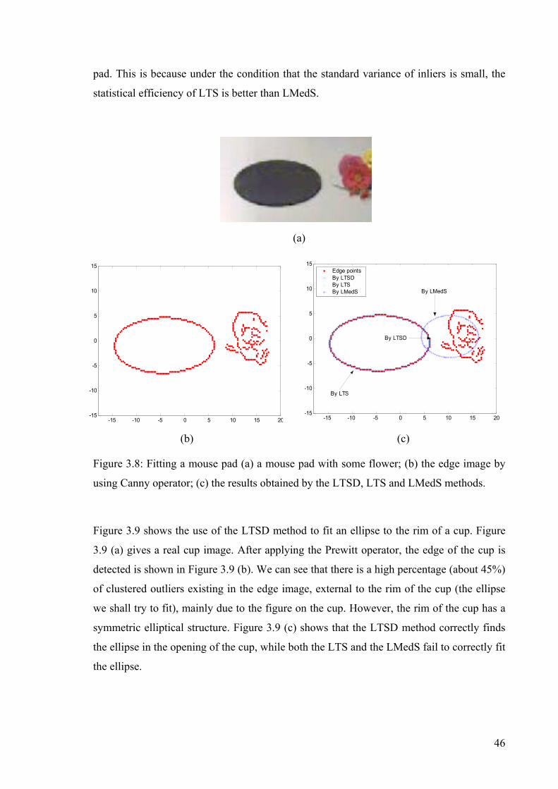
46
-15 -10 -5 0 5 10 15 20-15
-10
-5
0
5
10
15
-15 -10 -5 0 5 10 15 20-15
-10
-5
0
5
10
15Edge pointsBy LTSDBy LTSBy LMedS By LMedS
By LTS
By LTSD
pad. This is because under the condition that the standard variance of inliers is small, the
statistical efficiency of LTS is better than LMedS.
(a)
(b) (c)
Figure 3.8: Fitting a mouse pad (a) a mouse pad with some flower; (b) the edge image by
using Canny operator; (c) the results obtained by the LTSD, LTS and LMedS methods.
Figure 3.9 shows the use of the LTSD method to fit an ellipse to the rim of a cup. Figure
3.9 (a) gives a real cup image. After applying the Prewitt operator, the edge of the cup is
detected is shown in Figure 3.9 (b). We can see that there is a high percentage (about 45%)
of clustered outliers existing in the edge image, external to the rim of the cup (the ellipse
we shall try to fit), mainly due to the figure on the cup. However, the rim of the cup has a
symmetric elliptical structure. Figure 3.9 (c) shows that the LTSD method correctly finds
the ellipse in the opening of the cup, while both the LTS and the LMedS fail to correctly fit
the ellipse.

47
(a)
(b) (c)
Figure 3.9: Fitting the ellipse in a cup (a) a real cup image; (b) the edge of the cup by
applying Prewitt operator; (c) comparative results obtained by the LTSD, LTS and LMedS
methods
3.5.4 Experiments for Data with Uniform Outliers
Finally, we investigated the characteristics of the LTSD under uniform outliers. We
generated 200 data points with 40% uniform outliers (see Figure 3.10). The ellipse had a
standard variance 0.5, major axis 10.0, minor axis 8.0, center (0.0, 0.0), and orientation to
horizon direction θ is 0.0 degree. The uniform outliers were randomly distributed in a
rectangle with left upper corner (-20.0, 20.0) and right lower corner (20.0, -20.0). We
repeated the performance 100 times and the averaged results were shown in Table 3.2. We
can see the LTSD method can also work well in uniform outliers.
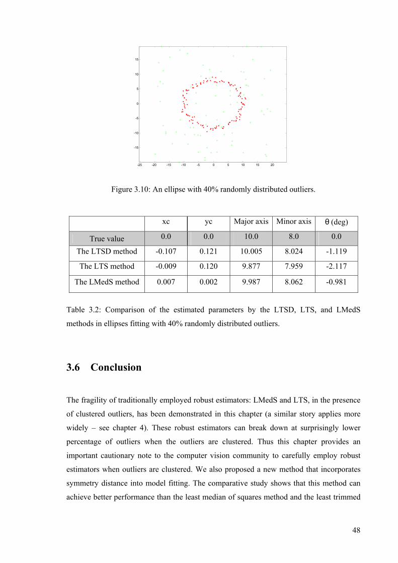
48
-25 -20 -15 -10 -5 0 5 10 15 20
-15
-10
-5
0
5
10
15
Figure 3.10: An ellipse with 40% randomly distributed outliers.
xc yc Major axis Minor axis θ (deg)
True value 0.0 0.0 10.0 8.0 0.0
The LTSD method -0.107 0.121 10.005 8.024 -1.119
The LTS method -0.009 0.120 9.877 7.959 -2.117
The LMedS method 0.007 0.002 9.987 8.062 -0.981
Table 3.2: Comparison of the estimated parameters by the LTSD, LTS, and LMedS
methods in ellipses fitting with 40% randomly distributed outliers.
3.6 Conclusion
The fragility of traditionally employed robust estimators: LMedS and LTS, in the presence
of clustered outliers, has been demonstrated in this chapter (a similar story applies more
widely – see chapter 4). These robust estimators can break down at surprisingly lower
percentage of outliers when the outliers are clustered. Thus this chapter provides an
important cautionary note to the computer vision community to carefully employ robust
estimators when outliers are clustered. We also proposed a new method that incorporates
symmetry distance into model fitting. The comparative study shows that this method can
achieve better performance than the least median of squares method and the least trimmed

49
squares method especially when large percentages of clustered outliers exist in the data and
the standard variance of inliers is large. The price paid for the improvement in fitting
models is an increase of the computational complexity due to the complicated definition of
symmetry distance. It takes about O(n2) time to compute symmetry distance (SD) for each
p-subset. The proposed method can be applied to the fitting of other symmetric shapes and
to other fields.
Unfortunately, LTSD was especially designed for spatially symmetric data distributions.
For inlier distributions that are not spatially symmetric (including structures that, though
they may be symmetric, have large amounts of missing or occluded data so that the visible
inliers are not symmetric), the LTSD is not a good choice (Note: for this kind of data, we
have developed other novel highly robust estimators that will be presented in the following
chapters). However, the LTSD does provide a feasible way to greatly improve the
achievements of conventional estimators –the LMedS and the LTS, especially, when the
data contain inliers (with symmetry) with large variance and are contaminated by large
percentage of clustered outliers.
In the next chapter, we will take advantage of the information in the structure of the pdf of
residuals, and propose a more general highly robust estimator: MDPE, which can be
widely applied in many computer tasks and is applicable for missing data, data with
occlusion, and data without symmetry. The same motivation is also behind several
improved methods: QMDPE and vbQMDPE (in chapter 5 and chapter 6).

50
4. MDPE: A Novel and Highly Robust Estimator
4.1 Introduction
Many robust estimators (such as M-estimators, LMedS, LTS, etc.) have been developed in
the statistics field. However, they assume that inliers occupy an absolute majority of the
whole data, and thus, they will breakdown for data involving an absolute majority of
outliers. Obviously, the requirement for 50% or more data belonging to inliers may not be
always satisfied, e.g., when the data contain multiple surfaces, when data from multiple
views are merged, or when there are more than 50% noise data points existing in the data.
For these cases, we need to find a more robust estimator that can tolerate more than 50%
outliers.
This chapter presents a novel robust estimator (MDPE). This estimator applies
nonparametric density estimation and density gradient estimation techniques in parametric
estimation (“model fitting”). The goals in designing MDPE are: it should be able to fit
signals corresponding to less than 50% of the data points and be able to fit data with multi-
structures. In developing MDPE, we make the common assumption that the residuals of
1.1.3. Chapter 4
MDPE: A Novel and Highly Robust Estimator

51
the inliers are contaminated by Gaussian noise (although the precise nature of the noise
distribution is not that essential, depending only upon zero mean and unimodality). We
also assume that the signal (we seek to fit) occupies a relative majority of the data – that is,
there are no other populations, belonging to valid structures, that singly has a larger
population. In other words, if there are multiple structures, we seek to fit the largest
structure (in terms of population of data – which is often related to but not necessarily
identical to geometric size). Of course, in a complete application of MDPE, such as the
range segmentation algorithm presented in the next chapter, one can apply the estimator
serially to identify the largest structured population, remove it, and then seek the largest in
the remaining population etc.
Key components of MDPE are: Probability Density estimation in conjunction with Mean
Shift techniques (Fukunaga and Hostetler 1975). The mean shift vector always points
towards the direction of the maximum increase in the probability density function (see
section 4.2). Through the mean shift iterations, the local maximum density, corresponding
to the mode (or the center of the regions of high concentration) of data, can be found.
MDPE optimizes an objective function that measures more than just the size of the
residuals. It considers the following two factors at the same time:
• The density distribution of the data points (in residual space) estimated by the
density estimation technique.
• The size of the residual corresponding to the local maximum of the probability
density distribution.
If the signal is correctly fitted, the densities of inliers should be as large as possible; at the
same time, the center of the high concentration of data should be as close to zero as
possible in the residual space. Thus, both the density distribution of data points in residual
space and the size of the residual corresponding to the local maximum of the density
distribution, are considered as important characteristics in the objective function of MDPE.
MDPE can tolerate a large percentage of outliers and pseudo-outliers (empirically, usually
more than 85%) and it can achieve better performance than other similar robust estimators.

52
To demonstrate the performance of MDPE, we compare, based upon tests on both
synthetic and real images, MDPE with other five popular robust estimators (from both
statistics and computer vision field): Hough Transform (HT), Random Sampling
Consensus (RANSAC), Least Median of Squares (LMedS), Residual Consensus (RESC),
and Adaptive Least kth Order Squares (ALKS). Experiments show that MDPE has a higher
robustness to outliers and fewer errors than the other five estimators.
The contributions of this chapter can be summarized as follows:
• We apply nonparametric density estimation and density gradient estimation
techniques in parametric estimation.
• We provide a novel estimator, MDPE, which can usually tolerate more than 85%
outliers although it is simple and easy to implement.
• The performance of MDPE has been compared with those of five other popular
methods, including “traditional” ones (RANSAC, Hough Transform, and LMedS)
and recently proposed ones (RESC and ALKS).
The organization of this chapter is as follows: density gradient estimation and the mean
shift method are introduced in section 4.2. Section 4.3 describes the MDPE method.
Comparative experimental results of MDPE and several other robust estimators are
contained in section 4.4. Finally, we conclude with a summary and a discussion of further
possible work in section 4.5.
4.2 Nonparametric Density Gradient Estimation and Mean
Shift Method
There are several nonparametric methods available for probability density estimation: the
histogram method, the naive method, the nearest neighbor method, and kernel estimation
(Silverman 1986). The kernel estimation method is one of the most popular techniques
used in estimating density. Given a set of n data points {Xi}i=1,…,n in a d-dimensional
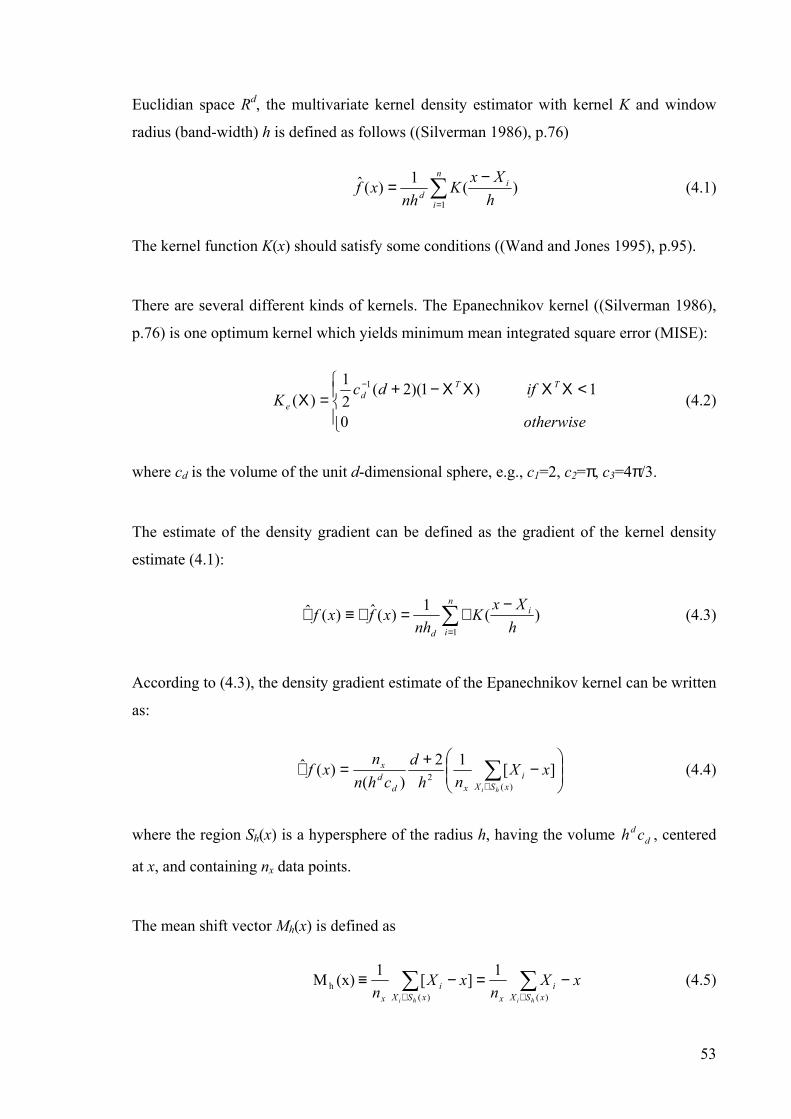
53
Euclidian space Rd, the multivariate kernel density estimator with kernel K and window
radius (band-width) h is defined as follows ((Silverman 1986), p.76)
∑=
−=
n
i
id h
XxK
nhxf
1)(1)(ˆ ( 4.1)
The kernel function K(x) should satisfy some conditions ((Wand and Jones 1995), p.95).
There are several different kinds of kernels. The Epanechnikov kernel ((Silverman 1986),
p.76) is one optimum kernel which yields minimum mean integrated square error (MISE):
<ΧΧΧΧ−+
=Χ−
otherwise
ifdcK
TTd
e
0
1)1)(2(21
)(1
( 4.2)
where cd is the volume of the unit d-dimensional sphere, e.g., c1=2, c2=π, c3=4π/3.
The estimate of the density gradient can be defined as the gradient of the kernel density
estimate ( 4.1):
∑=
−∇=∇≡∇
n
i
i
d hXx
Knh
xfxf1
)(1)(ˆ)(ˆ ( 4.3)
According to ( 4.3), the density gradient estimate of the Epanechnikov kernel can be written
as:
−+=∇ ∑
∈ )(2 ][12
)()(ˆ
xSXi
xddx
hi
xXnh
dchn
nxf ( 4.4)
where the region Sh(x) is a hypersphere of the radius h, having the volume dd ch , centered
at x, and containing nx data points.
The mean shift vector Mh(x) is defined as
xXn
xXn xSX
ixxSX
ix hihi
−=−≡ ∑∑∈∈ )()(
h1][1 (x)M ( 4.5)
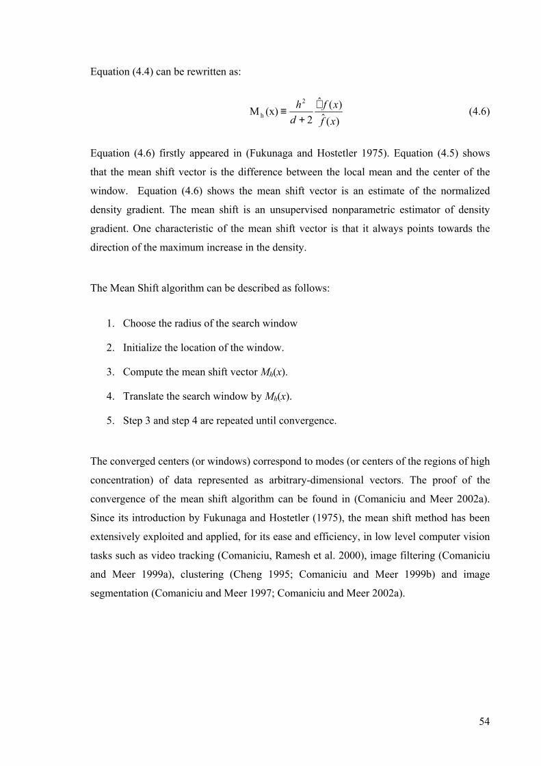
54
Equation ( 4.4) can be rewritten as:
)(ˆ)(ˆ
2 (x)M
2
hxfxf
dh ∇+
≡ ( 4.6)
Equation ( 4.6) firstly appeared in (Fukunaga and Hostetler 1975). Equation ( 4.5) shows
that the mean shift vector is the difference between the local mean and the center of the
window. Equation ( 4.6) shows the mean shift vector is an estimate of the normalized
density gradient. The mean shift is an unsupervised nonparametric estimator of density
gradient. One characteristic of the mean shift vector is that it always points towards the
direction of the maximum increase in the density.
The Mean Shift algorithm can be described as follows:
1. Choose the radius of the search window
2. Initialize the location of the window.
3. Compute the mean shift vector Mh(x).
4. Translate the search window by Mh(x).
5. Step 3 and step 4 are repeated until convergence.
The converged centers (or windows) correspond to modes (or centers of the regions of high
concentration) of data represented as arbitrary-dimensional vectors. The proof of the
convergence of the mean shift algorithm can be found in (Comaniciu and Meer 2002a).
Since its introduction by Fukunaga and Hostetler (1975), the mean shift method has been
extensively exploited and applied, for its ease and efficiency, in low level computer vision
tasks such as video tracking (Comaniciu, Ramesh et al. 2000), image filtering (Comaniciu
and Meer 1999a), clustering (Cheng 1995; Comaniciu and Meer 1999b) and image
segmentation (Comaniciu and Meer 1997; Comaniciu and Meer 2002a).

55
-4 -2 0 2 4 6 8 0
0.02
0.04
0.06
0.08
0.1
0.12
0.14
0.16
0.18
0.2
Two mode normal Distribution
Pro
babi
lity
Den
sity
P0
P0'
P1
P1'
Figure 4.1: One example where the mean shift estimator found the local maximum of the
probability densities.
To illustrate the mean shift method, two sets of samples from normal distributions were
generated, each having 1000 data points and with unit variance. One had a distribution
with zero mean, and the other had a mean of 4.0 (see Figure 4.1). These points were
distributed along the abscissa but here we choose to plot only the corresponding
probability density at those data points). We selected two initial points as the centers of the
initial windows: P0 (-2.0) and P1 (2.5). The search window radius was chosen as 1.0. After
applying the mean shift algorithm, the mean shift estimator automatically found the local
maximum densities (the centers of converged windows). Precisely, P0’ located at -0.0305,
and P1’ with 4.0056. The centers (P0’ and P1’) of the converged windows correspond to
the local maximum probability densities, that is, the two modes.

56
4.3 Maximum Density Power Estimator—MDPE
4.3.1 The Density Power (DP)
Random sampling techniques have been widely used in a lot of methods, for example,
RANSAC, LMedS, RESC, ALKS, etc (see chapter 2). Each uses the random sampling
techniques to choose p points, called a p-subset, to determine the parameters of a model for
that p-subset (p equals 2 for a line, 3 for a circle or plane, 6 for a quadratic curve), and
finally outputs the parameters determined by the p-subset with the minimum or maximum
of the respective objective function. They differ in their objective functions used to rank
the p-subsets. Here we define a new objective function.
When a model is correctly fitted, there are two criteria that should be satisfied:
(1) Data points on or near the model (inliers) should be as many as possible;
(2) The residuals of inliers should be as small as possible.
Most objective functions of existing methods consider either one of the criteria or both.
RANSAC (Fischler and Rolles 1981) applies criterion (1) into its optimization process and
outputs the results with the highest number of data points within an error bound; The Least
squares method uses criterion (2) as its objective function, but minimizes the residuals of
all data points without the ability to differentiate the inliers from the outliers; MUSE,
instead of minimizing the residuals of inliers, minimizes the scale estimate provided by the
kth ordered absolute residual. RESC combines both criteria into its objective function, i.e.,
the histogram power. Among all these methods, RESC obtains the highest breakdown
point. It seems that it is preferable to consider both criteria in the objective function.
The new estimator we introduce here, MDPE, also considers these two criteria in its
objective function. We assume the residuals of the inliers (good data points) satisfy a zero
mean, smooth and unimodal distribution: e.g., a Gaussian-like distribution. If the model to
fit is correctly estimated, the data points on or near the fitted structure should have a higher
probability density; and at the same time, the center of the converged window by the mean
shift procedure (corresponding to the highest local probability density) should be as close

57
to zero as possible in residual space. According to the above assumptions, our objective
function ψDP considers two factors: (1) the densities f (Xi) of all data points within the
converged window Wc and (2) the center Xc of the converged window. Thus ψDP
∑∈
∝Wc
)(ˆiX
iXf and ψDP Xc1∝ . We define the probability density power function as
follows:
)exp(
)(ˆ
Xc
Xfci WX
i
DP
α
ψ
=∑∈ ( 4.7)
where Xc is the center of the converged window Wc obtained by applying the mean shift
procedure. α is a factor that adjusts the relative influence of the probability density to the
residual of the point corresponding to the center of the converged window. α is
empirically set to 1.0. Experimentally, we have found the above form to behave better than
various other alternatives having the same general form.
If a model is found, Xc is very small, and the densities within the converged window are
very high. Thus our objective function will produce a high score. Experiments, presented
in the next section, show that MDPE is a very powerful method for data with a large
percentage of outliers.
4.3.2 The MDPE Algorithm
As Lee stated (Lee, Meer et al. 1998), any one-step robust estimator cannot have a
breakdown point exceeding 50%, but estimators adopting multiple-step procedures with an
apparent breakdown point exceeding 50% are possible.
MDPE adopts a multi-step procedure. The procedure of MDPE can be described as
follows:
(1) Choose a search window radius h, and a repetition count m. The value m can be
chosen according to equation ( 2.23).

58
(2) Randomly choose one p-subset, estimate the model parameters by the p-subset,
and calculate the signed residuals of all data points.
(3) Apply the mean shift steps in the residual space with initial window center zero.
Notice that the mean shift is employed in one-dimensional space – signed residual
space. The converged window center C can be obtained by the mean shift
procedure in section 4.2.
(4) Calculate the densities (using equation 4.1) corresponding to the positions of all
data points within the converged window with radius h in the residual-density
space.
(5) Calculate the density power according to equation ( 4.7).
(6) Repeat step (2) to step (5) m times. Finally, output the parameters with the
maximum density power.
The results are from one p-subset, corresponding to the maximum density power. In order
to improve the statistical efficiency, a weighted least square procedure [(Rousseeuw and
Leroy 1987), p.202] is carried out after the initial MDPE fit. However, a more robust scale
estimator TSSE (which was proposed at the later stage—see chapter 7) can also be
employed.
Instead of estimating the fit involving the absolute majority in the data set, MDPE finds a
fit having a relative majority of the data points. This makes it possible, in practice, for
MDPE to obtain a high robustness that can tolerate more than 50% outliers.
4.4 Experiments and Analysis
Next, we will compare the abilities of several estimators (MDPE, RESC, ALKS, LMedS,
RANSAC, and Hough Transform) to deal with data with a large percentage of outliers. We
choose RANSAC and Hough Transform as two methods to compare with, because they are
very popular methods and have been widely applied in computer vision. Provided with the
correct error tolerance (for RANSAC) or bin size (for Hough Transform), they can tolerate

59
more than 50% outliers. Although LMedS has only 0.5 breakdown point and cannot
tolerate more than 50% outliers, it needs no prior knowledge of the variance of inliers.
RESC and ALKS are two relatively new methods and represent modern developments in
robust estimation. We also note that RANSAC, LMedS, RESC, ALKS, and MDPE all
adopt similar four-step procedures: randomly sampling; estimating the parameter candidate
for each sample; evaluating the quality of each candidate; outputting the final parameter
estimate with the best quality measure.
In this section, we will investigate the characteristics of the six methods under clustered
outliers and different percentages of outliers. We also investigate the time complexity of
the five comparative methods (LMedS, RANSAC, ALKS, RESC, and MDPE). We
produce the breakdown plot of the six methods, and test the influence of the choice of
window radius on the MDPE. Unless we specify, the window radius h for MDPE will be
set at 2.0 for the experiments in this section.
4.4.1 Experiment 1
In this experiment, the performance of MDPE in line fitting and circle fitting will be
demonstrated and its tolerance to large percentages of outliers will be compared with five
other popular methods: RANSAC, Hough Transform, LMedS, RESC, and ALKS. The
time complexity of the five methods (except for Hough Transform) will also be evaluated
and compared. We will show that some methods break down. We can (and have) checked
whether such a breakdown is an artifact of implementation (e.g. randomly sampling) or
whether the breakdown is the result of the objective function for that method scoring
wrong fit “better” than the true one—see discussions later (sub-section 4.4.1.1) .
4.4.1.1 Line Fitting
We generated four kinds of data (step, three-step, roof, and six-line), each with a total of
500 data points. The signals were corrupted by Gaussian noise with zero mean and
standard variance σ. Among the 500 data points, α data points were randomly distributed
in the range of (0, 100). The i'th structure has ni data points.
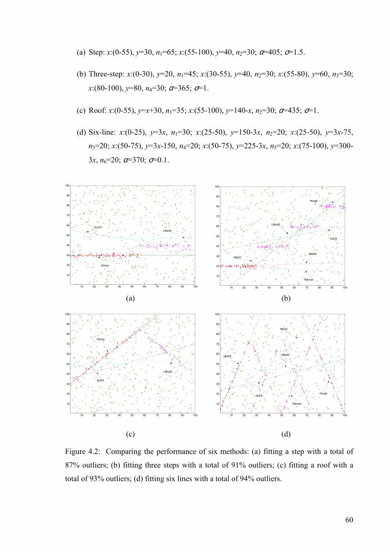
60
10 20 30 40 50 60 70 80 90 100
10
20
30
40
50
60
70
80
90
100
ALKS LMedS
Others
10 20 30 40 50 60 70 80 90 100
10
20
30
40
50
60
70
80
90
100
ALKS
LMedS
MDPE
Ransac
RESC
Hough
10 20 30 40 50 60 70 80 90 100
10
20
30
40
50
60
70
80
90
100
ALKS
LMedS
Others
10 20 30 40 50 60 70 80 90 100
10
20
30
40
50
60
70
80
90
100
ALKS
LMedS MDPE
Ransac
RESC
Hough
(a) Step: x:(0-55), y=30, n1=65; x:(55-100), y=40, n2=30; α=405; σ=1.5.
(b) Three-step: x:(0-30), y=20, n1=45; x:(30-55), y=40, n2=30; x:(55-80), y=60, n3=30;
x:(80-100), y=80, n4=30; α=365; σ=1.
(c) Roof: x:(0-55), y=x+30, n1=35; x:(55-100), y=140-x, n2=30; α=435; σ=1.
(d) Six-line: x:(0-25), y=3x, n1=30; x:(25-50), y=150-3x, n2=20; x:(25-50), y=3x-75,
n3=20; x:(50-75), y=3x-150, n4=20; x:(50-75), y=225-3x, n5=20; x:(75-100), y=300-
3x, n6=20; α=370; σ=0.1.
(a) (b)
(c) (d)
Figure 4.2: Comparing the performance of six methods: (a) fitting a step with a total of
87% outliers; (b) fitting three steps with a total of 91% outliers; (c) fitting a roof with a
total of 93% outliers; (d) fitting six lines with a total of 94% outliers.

61
From Figure 4.2, we can see that because LMedS has only a 0.5 breakdown point, it cannot
resist more than 50% outliers. Thus, LMedS failed to fit all the four signals; The ALKS,
RESC and MDPE approaches all have higher robustness, compared with LMedS, to
outliers. However, the results show that ALKS is not applicable for the signals with such
large percentages of outliers because it failed in all four cases. RESC, although having a
very high robustness, fitted one model, but failed three. The Hough Transform could not
correctly fit the step signals, which happen to fall near an inclined line, with large
percentages of outliers. Provided with the correct error bound of inliers, RANSAC
correctly fitted three signals, but failed one. Only the MDPE method correctly fitted all the
four signals. The MDPE didn’t breakdown even with 94% outliers. In Figure 4.2 (d), we
can see, although MDPE, Hough Transform, and RANSAC did not breakdown, they found
different lines in the six-line signal (according to their own criterion).
Among these six methods, MDPE, RESC and RANSAC are similar to each other. They all
randomly choose p-subsets and try to estimate parameters by a p-subset corresponding to
the maximum value of their object function. Thus, their objective functions are the core
that determines how much robustness to outliers these methods have. RANSAC considers
only the number of data points falling into given error bound of inliers; RESC considers
the number of data points within the mode and the residual distributions of these points;
MDPE considers not only the density distribution of the mode, which is assumed having
Gaussian-like distribution, in the residual space, but also the size of the residual
corresponding to the center of the mode.
It is important to point out that the failures of RESC, ALKS, LMedS, and RANSAC, and
Hough Transform in some of or all of the four signals is inherent and not simply an artefact
of our implementation. Let us check the criteria of RESC and we will understand why
RESC failed to fit to the three signals. The objective function of RESC for the correct fit is
7.0 (for one-step signal), 5.8 (for three-steps signal) and is 4.4 (for six-lines signal).
However, the objective function of RESC for the estimated parameters is 7.6 for a step, 8.1
for three steps and 5.3 the six-line signal. In fact, during the searching procedure, the
RESC estimator consistently maximizes its objective function—histogram power, starting
with initial fits that have a smaller histogram power, but successively finding fits with
higher histogram power – proceeding to even higher histogram power than that possessed
by the true fit. The failures of RANSAC, LMedS and ALKS have a similar nature: for

62
example, the median of residuals of the true fit is 16.8, 29.2 and 97.0 for a step, three steps
and six lines respectively. However the median of residuals of final result by the LMedS
method is 16.3, (for a step), 15.5 (for three steps) and 23.4 (for six lines). The problem is
not with the implementation but with the criterion.
4.4.1.2 Circle Fitting
The proposed MDPE is a general method that can be easily applied to fit other kinds of
models, such as circles, ellipsis, planes, etc. Figure 4.3 shows the ability of the MDPE to fit
circles under 95% outliers. Five circles were generated, each with 101 data points and
σ=0.1. 1500 random outliers were distributed within the range (-75, 75). Thus, for each
circle, it has 1904 outliers (404 pseudo-outliers plus 1500 random outliers). The MDPE
method gave more accurate results than LMedS, RESC, and ALKS. The Hough
Transform and RANSAC also correctly fit the circles when provided with correct bin size
(for Hough Transform) and error bound of inliers (for RANSAC). The three methods
(MDPE, Hough Transform, and RANSAC) fitted three different circles according to their
own criterion.
Figure 4.3: One example of fitting circles by the six methods. The data had about 95%
outliers.

63
4.4.1.3 Time Complexity
It might be interesting to compare the time complexity between the different methods. In
this experiment, we will compare the speed of MDPE, RESC, ALKS, LMedS, and
RANSAC. We do not consider the Hough Transform, because the speed of Hough
transform depends on the dimension of parameter space, the range of each parameter, and
the bin size. It also uses a different framework (voting in parameter space), compared with
the other five methods (which use sampling techniques).
In order to make the speed of each method comparable, the same simple random sampling
technique was used for all five methods. Although some other sampling techniques exist,
such as guided sampling (Tordoff and Murray 2002) and GA sampling (Roth and Levine
1991; Yu, Bui et al. 1994), and the speed of each method by adopting these sampling
techniques can be improved; we adopted the simple randomly sampling technique because:
(1) It has been widely used in most robust estimators (such as LMedS, LTS,
RANSAC, ALKS, MUSE, MINPRAN, etc.).
(2) It is easy to perform.
A Step Three Steps A Roof Six Lines Five Circles
Percentages of outliers 87% 91% 93% 94% 95%
Number of Sampling: m 500 1000 1500 2000 3000
MDPE 7.3 15.1 20.1 28.4 73.4
RESC 12.6 23.8 35.4 47.3 82.2
ALKS 6.4 13.7 19.8 26.7 126.8
LMedS 0.6 1.3 2.0 3.0 14.6
RANSAC 0.7 1.2 1.6 2.5 14.0
Table 4.1: The comparison of time complexity for the five methods (all time in seconds).

64
We used the signals above (a step, three steps, a roof, six lines, and five circles) to test
speed of the five methods. We repeated the experiments on each signal 10 times, and the
mean time of each method for each signal was recorded. We performed them all in
complete MATLAB code (programming in C code with optimisation will make the
methods faster).
From Table 4.1, we can see that LMedS and RANSAC have similar speed and they are
faster than MDPE, RESC, and ALKS. MDPE is about 35% faster than RESC. The speed
of MDPE is close to that of ALKS in line fitting but faster than ALKS in the five-circles
fitting. ALKS is also faster than RESC in line fitting, but slower than RESC in circle
fitting. We noted that the time complexity of ALKS, compared with MDPE and RESC, is
higher in the five-circle signal (2005 data points) than in the line signals (505 data points).
This is because the ALKS procedure used m p-subsets for each value of k (as
recommended by Lee and Meer, the number of different k is equal to 19). Thus, when the
number of data points and sampling times is increased, the increase of time complexity of
ALKS in sorting the residuals of the data points (mainly) is higher than that of RESC in
compressing histogram, and that of MDPE in calculating density power.
4.4.2 Experiment 2
In the previous experiment, we investigated the characteristics of the six methods to fit
data with multiple structures. In this experiment, we will explore the abilities of the six
methods to fit data with clustered outliers. We generated a line (y=x-1) corrupted by
Gaussian noise with zero mean and standard variance σ1. The line had n data points.
Among the total 500 data points, α data points were randomly distributed in the range of
(0, 100.0), and β clustered outliers were added to the signals, possessing a spherical
bivariate normal distribution with standard variance σ2 and mean (80.0, 30.0).
(a) γ=100, σ1=1.0; α=200; β=200; σ2=5.0.
(b) γ=100, σ1=1.0; α=200; β=200; σ2=2.0.
(c) γ=275, σ1=1.0; α=0; β=225; σ2=1.0.
(d) γ=275, σ1=5.0; α=0; β=225; σ2=1.0.

65
10 20 30 40 50 60 70 80 90 100
10
20
30
40
50
60
70
80
90
100
LMedS
Others
10 20 30 40 50 60 70 80 90 100
10
20
30
40
50
60
70
80
90
100
Hough
RESC
LMedS
MDPE and RANSAC
ALKS
(a) (b)
(c) (d)
Figure 4.4: Experiment where the six methods are fitting a line with clustered outliers. The
standard variance of both clustered outliers and inliers will affect the results of the six
methods.
Figure 4.4 shows that both the standard variance of clustered outliers σ2 and the standard
variance of inliers to the line σ1 will decide the accuracy of the results estimated by the six
methods. When σ1 is small and σ2 is large, all methods except for LMedS can correctly fit
the line although a large number of clustered outliers existed in the data (see Figure 4.4
(a)). The LMedS failed because it cannot tolerate more than 50% outliers. When the
standard variance of clustered outliers is small, i.e., the outliers are densely clustered
within a small range; the ability of MDPE, RESC, ALKS, and RANSAC to resist the
influence of clustered outliers will be greatly reduced (see Figure 4.4 (b)). As shown in
Figure 4.4 (c) and Figure 4.4 (d), the standard variance of inliers to the line will also affect
10 20 30 40 50 60 70 80 90 100
10
20
30
40
50
60
70
80
90
100
Others
RESC
10 20 30 40 50 60 70 80 90 100
10
20
30
40
50
60
70
80
90
100
RESC
Hough
ALKS
MDPE
LMedS and RANSAC
66
the accuracy of the results by LMedS, MDPE, RESC, ALKS, and RANSAC. When σ1 was
5.0 (Figure 4.4 (d)), all the five methods failed to fit the line even with only 45% clustered
outliers.
The Hough Transform, to our surprise, showed excellent performance to resist clustered
outliers. It succeeded to fit all the four signals despite clustered outliers. We note that the
Hough Transform adopts a different framework to the other five methods: it uses a voting
technique in parameter spaces instead of residual space. It would seem that the objective
functions of all other methods fail to score the correct solutions highly (for MDPE, RESC,
and RANSAC) or lowly (for LMedS and ALKS) enough when there are large numbers of
very highly clustered outliers. This has been noted before with the LMedS (Wang and
Suter 2003a; also see chapter 3) and is presumably one reason why the proofs of high
breakdown point specifically stipulates rather generally distributed outliers.
4.4.3 Experiment 3
It is important to know the characteristics of the various methods when the signals were
contaminated by different percentages of outliers. In this experiment, we will draw the
“breakdown plot” and compare the abilities of the six methods to resist different
percentages of outliers (in order to avoid crowding, each sub-figure in Figure 4.5 includes
three methods). We generated step signals (y=Ax+B) as follows:
Signals: line 1: x:(0-55), A=0, B=30, n1 will be decreased with the increase of uniformly
distributed outliers α; line 2: x:(55-100), A=0, B=60, n2=25; for both lines: σ=1.
In total 500 points. 15 clustered outliers centred at (80, 10) with unit variance were added
to the signals. At the beginning, n1 = 460, α=0, so the first signal had an initial 8% outliers;
then every repetition of the experiment 5 points were moved from n1 to uniform outliers
(α) ranging over (0-100) until n1=25. Thus the percentage of outliers in the data points
changed from 8% to 95%. The whole procedure above was repeated 20 times.

67
10 20 30 40 50 60 70 80 90 100-20
-15
-10
-5
0
5
10
15
20
Outliers Percentage
Erro
r in
B
MPDERESCRANSAC
10 20 30 40 50 60 70 80 90 100
-0.25
-0.2
-0.15
-0.1
-0.05
0
0.05
0.1
0.15
0.2
0.25
Outliers Percentage
Erro
r in
A
MDPE RESC RANSAC
10 20 30 40 50 60 70 80 90 100
-0.25
-0.2
-0.15
-0.1
-0.05
0
0.05
0.1
0.15
0.2
0.25
Outliers Percentage
Erro
r in
A
ALKS LMedS Hough
10 20 30 40 50 60 70 80 90 100-20
-15
-10
-5
0
5
10
15
20
Outliers Percentage E
rror i
n B
ALKSLMedSHough
As Figure 4.5 illustrated, the LMedS first broke down (at about 50% of outliers) among all
these six estimators. ALKS broke down even when outliers comprised less than 80%;
RESC began to break down when outliers comprised more than 88% of the total data.
(a1) (b1)
(a2) (b2)
Figure 4.5: Breakdown plot for the six methods: (a1) and (a2) error in A vs. outlier
percentage; (b1) and (b2) error in B vs. outlier percentage.
From Figure 4.5, we can also see that, provided with the correct error bound (for
RANSAC) and with a “good” bin size (for Hough Transform), RANSAC and Hough
Transform can tolerant more than 50% outliers. RANSAC began to break down at 92%
outliers; Hough transform began to break down when outliers have more than 88% (broke
down at 89% or more outliers). However, the performance of RANSAC is largely
dependent on the correct choice of error tolerance. If the error tolerance deviated from the
correct error tolerance, RANSAC will completely breakdown (see the experiment in

68
subsection 4.4.4.2). Similarly, the good performance of the Hough Transform is largely
dependent on the choice of accumulator bin size. If the bin size is wrongly given, Hough
Transform will also breakdown (this phenomenon was also pointed out by Chen and Meer
(Chen and Meer 2002)).
In contrast, MDPE has the highest robustness among the six methods. MDPE began to
break down only at 94% outliers. However, even at 94% and 95% outliers, MDPE had
still, loosely speaking, about 75% correct estimation rate out of the 20 times.
Another thing we noticed is that ALKS has some obvious fluctuations in the results when
the outliers are less than 30%, while the other five do not have this undesirable
characteristic. This may be because the robust estimate of the noise variance is not valid
for small or large k values (k is the optimum value to be determined by the data).
Among all these six methods, MDPE and RANSAC have similar accuracy. They are more
accurate than RESC, ALKS, and LMedS. The accuracy of the Hough Transform greatly
depends on the accumulator bin size in each parameter space. Generally speaking, the
larger the bin size is, the lower accuracy the Hough Transform may have. Thus, in order to
obtain higher accuracy, one needs to reduce the bin size. However, this will lead to an
increase in storage requirements and computational complexity. Also, one can have a bin
size that is too small (theoretically, each bin receives less votes and in the limit of very
small bin size, no bin will have more than 1 vote!).
4.4.4 Experiment 4
The problem of the choice of window radius in the means shift, i.e., bandwidth selection,
has been widely investigated during the past decades (Silverman 1986; Wand and Jones
1995; Comaniciu, Ramesh et al. 2001; Comaniciu and Meer 2002a). Comaniciu and Meer
(2002a) suggested several techniques for the choice of window radius:
1. The optimal bandwidth should be the one that minimizes AMISE;

69
0 2 4 6 8 10 12 14 16 18 20-0.1
0
0.1
0.2
0.3
0.4
0.5
0.6
Window Radius H
Erro
r in
A
50% Outliers 60% Outliers 70% Outliers 80% Outliers
0 2 4 6 8 10 12 14 16 18 200
2
4
6
8
10
12
Window Radius H
Errr
o in
B
50% Outliers60% Outliers70% Outliers80% Outliers
2. The choice of the bandwidth can be taken as the center of the largest operating
range over which the same results are obtained for the same data.
3. The best bandwidth maximizes a function that expresses the quality of the results.
4. User provides top-down information to control the kernel bandwidth.
Next we will investigate the influence of the choice of window radius on the results of
MDPE.
4.4.4.1 The Influence of the Window Radius and the Percentage of Outliers on
MDPE
Figure 4.6: The influence of window radius and percentage of outliers on the results of the
MDPE.
Although the MDPE has showed its powerful ability to tolerate large percentage of outliers
(including pseudo-outliers), its success is decided by the correct choice of window radius
h. If h is chosen too small, it is possible that the densities of data points in the residual
space may not be correctly estimated (the density function is a noisy function with many
local peaks and valleys), and some inliers may possibly be neglected; on the other hand, if
h is set too large, the window will include all the data points including inliers and outliers;
all peaks and valleys of the density function will also be smoothed out. In order to
investigate the influence of the choice of window radius h and percentage of outliers on the
estimated results, we generated a step signal: y=Ax+B, where A=0, B=30 for x:(0-55),

70
n1=100; and A=0, B=70 for x:(55-100), n2=80. . The step was corrupted by Gaussian noise
with a unit variance. In total, 500 data points were generated. Uniformly distributed
outliers in the range (0-100) were added to the signal so that the data respectively included
50%, 60%, 70% and 80% outliers (including uniformly distributed outliers and pseudo
outliers). To investigate the effect of window size in MDPE, the window radius h was set
from 1 to 20 with increasing step by 1 each time. The results were repeated 20 times.
Figure 4.6 shows that the absolute errors in A and B increase with the window radius h
(when h is larger than some range) because when the radius becomes larger, it is possible
that more outliers were included within the converged window. The percentage of outliers
has influence on the sensitivity of the results to the choice of window radius: when the data
include a higher percentage of outliers, the results are relatively more sensitive to the
choice of window radius; in contrast, when there are a less percentage of outliers in the
data, the results are relatively less sensitive to the choice the window radius.
4.4.4.2 The Influence of the Choice of Error Tolerance on RANSAC
We notice that RANSAC has an important parameter—error tolerance (i.e. error bound of
inliers), the correct choice of which is crucial for the method’s success in model fitting.
The purpose of error tolerance in RANSAC has some similarity to the window radius h in
MDPE: they both restrict immediate consideration of the data within some range; MDPE
uses the densities of the data within the converged window; RANASC uses the number of
the data within error tolerance. It would be interesting to investigate the sensitivity of the
results to the choice of the error bounds in RANSAC. We used the same signal as used in
Figure 4.6 and the results were repeated 20 times.
As Figure 4.7 show, RANSAC has little robustness to the choice of different error bound.
When the error bound deviated from the true value (which is assumed as a priori
knowledge), RANSAC totally broke down. Moreover, the result of RANSAC is very
sensitive the choice of error bound, regardless of the percentages of outliers that are
included in the data: even when the data included 50% outliers, RANSAC still broke down
when the wrong error bound was provided. This is different to the behaviour of MDPE. As
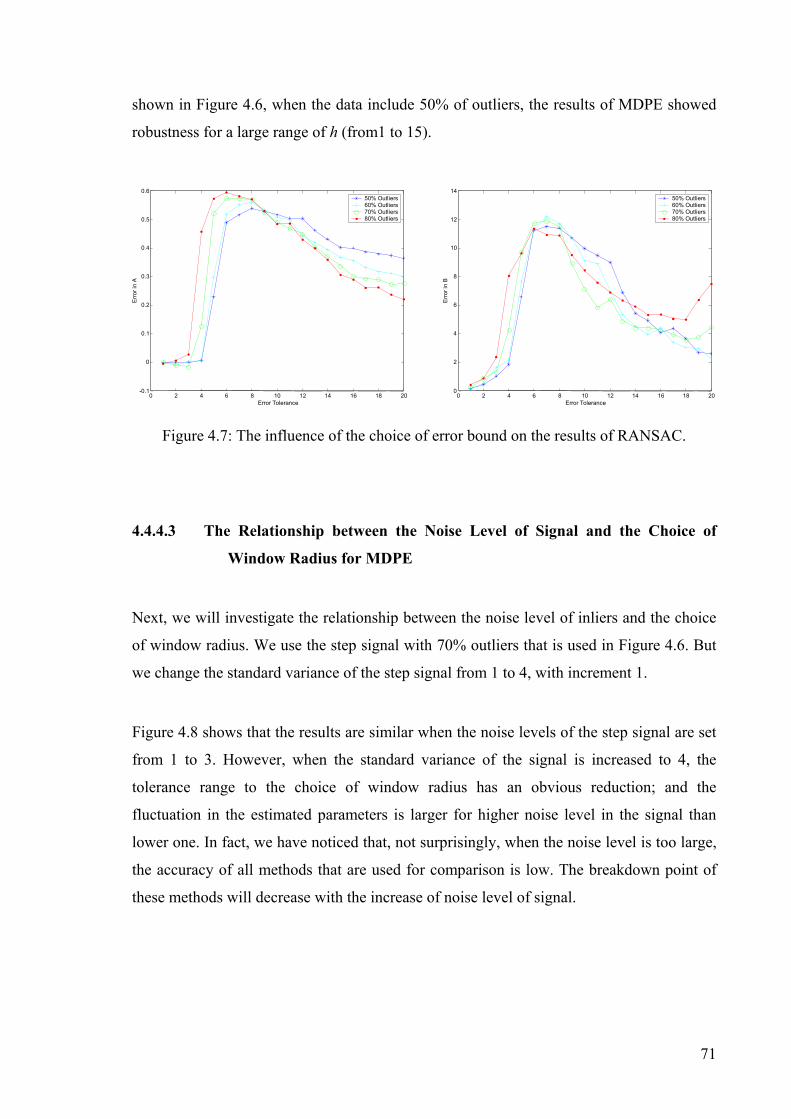
71
shown in Figure 4.6, when the data include 50% of outliers, the results of MDPE showed
robustness for a large range of h (from1 to 15).
Figure 4.7: The influence of the choice of error bound on the results of RANSAC.
4.4.4.3 The Relationship between the Noise Level of Signal and the Choice of
Window Radius for MDPE
Next, we will investigate the relationship between the noise level of inliers and the choice
of window radius. We use the step signal with 70% outliers that is used in Figure 4.6. But
we change the standard variance of the step signal from 1 to 4, with increment 1.
Figure 4.8 shows that the results are similar when the noise levels of the step signal are set
from 1 to 3. However, when the standard variance of the signal is increased to 4, the
tolerance range to the choice of window radius has an obvious reduction; and the
fluctuation in the estimated parameters is larger for higher noise level in the signal than
lower one. In fact, we have noticed that, not surprisingly, when the noise level is too large,
the accuracy of all methods that are used for comparison is low. The breakdown point of
these methods will decrease with the increase of noise level of signal.
0 2 4 6 8 10 12 14 16 18 20-0.1
0
0.1
0.2
0.3
0.4
0.5
0.6
Error Tolerance
Erro
r in
A
50% Outliers60% Outliers70% Outliers80% Outliers
0 2 4 6 8 10 12 14 16 18 200
2
4
6
8
10
12
14
Error Tolerance
Erro
r in
B
50% Outliers60% Outliers70% Outliers80% Outliers

72
LMedS
ALKS
Others
Figure 4.8: The relationship between the noise level of signal and the choice of window
radius in MDPE.
4.4.5 Experiments on Real Images
(a) (b)
(c)
Figure 4.9: Fitting a line (a) one real pavement; (b) the edge image obtained by using
Canny operator; (c) the results of line fitting obtained by the six methods.
0 2 4 6 8 10 12 14 16 18 200
0.1
0.2
0.3
0.4
0.5
0.6
0.7
Window Radius H
Erro
r in
A
σ =1σ =2σ =3σ =4
0 2 4 6 8 10 12 14 16 18 200
2
4
6
8
10
12
Window Radius H
Erro
r in
B
σ =1σ =2σ =3σ =4

73
0 50 100 150 200 250
20
40
60
80
100
120
140
160
180
200
220
In this experiment, we will provide two real images to show the ability of MDPE to
tolerate large percentage of outliers.
The first example is to fit a line in the pavement shown in Figure 4.9. The edge image was
obtained by using Canny operator with threshold 0.15 and included 2213 data points
(shown in Figure 4.9 (b)). There were about 85% outliers (most belonging to pseudo-
outliers which had structures and belonged to other lines) in the data. Six methods (MDPE,
RESC, ALKS, LMedS, RANSAC, and Hough Transform) were applied to fit a line in the
pavement. As shown in Figure 4.9 (c), ALKS and LMedS failed to correctly fit a line in
the pavement; while the other four methods correctly found a line.
(a) (b)
(c)
Figure 4.10: Fitting a circle edge. (a) twelve cups; (b) the edge image obtained by using
Canny operator; (c) the results of circle fitting obtained by the six methods.
74
The second example is to fit a circlar edge of one cup out of twelve cups. Among the total
1959 data points, the inliers corresponding to each cup were less than 10% of the total data
points. This is another multiple-solution case: the fitted circle can correspond to any cup in
the twelve cups. As shown in Figure 4.10, MDPE, RANSAC, and Hough Transform all
correctly found a cup edge (the result of RANSAC was relatively lower in accuracy than
that of MDPE), but each method found a different circle (Note: as these are not synthetic
data, we do not have the correct error bound for RANSAC and bin size for Hough
Transform. We empirically chose the error bound for RANSAC and bin size for Hough
Transform so that the performance was optimized). However, all other three methods
(RESC, ALKS, and LMedS), which are closer to MDPE in spirit, failed to fit the circle
edge of a cup.
4.5 Conclusion
In this chapter, we introduced a new and highly robust estimator (MDPE). MDPE is
similar to many random sampling estimators: we randomly choose several p-subsets, and
we calculate the residuals for the fit determined by each p-subset. However, the crux of the
method is that we apply the mean shift procedure to find the local maximum density of
these residuals. Furthermore, we evaluate a density power measure involving this
maximum density. The final estimated parameters are those determined by the one p-
subset corresponding to the maximum density power over all of the evaluated p-subsets.
Our method, and hence our definition of maximum density power, is based on the
assumption that when a model is correctly fitted, its inliers in residual space should have a
higher probability density, and the residual at the maximum probability density of inliers
should have a low absolute value. This captures the dual notions that: the data points
having lower residuals should be as many as possible, and that the residuals should be as
small as possible. In that sense, our method combines the essence of two popular
estimators: Least Median of Squares (low residuals) and RANSAC (maximum number of
inliers). However, unlike RANSAC, MDPE scores the results by the densities of data
points falling into the converged window and on the size of residual of the point
corresponding to local maximum density. Contrast this also with the Least Median of
Squares, which uses a single statistic (the median).

75
The result of our innovation is a highly robust estimator. The MDPE can tolerate more than
85% outliers, and has regularly been observed to function well with even more than 90%
outliers.
We also compared our method with several traditional (RANSAC, Hough Transform and
LMedS) and recently provided methods (RESC and ALKS). From our experimental
analysis, it is hard to say if any method has a clear advantage. LMedS and RANSAC are
the fastest among the six methods. However, the apparent breakdown point of LMedS is
lower; and RANSAC needs a priori knowledge of the error bounds. The results of
RANSAC are very sensitive the choice of error bounds, even when the percentage of
outliers is low. The Hough Transform shows excellent performance when the data include
clustered outliers. However, the space requirement and time complexity is high when the
dimension of parameters is high and high accuracy is required. Among recently proposed
estimators: MDPE, RESC, and ALKS; MDPE has the highest robustness to outliers. ALKS
shows less robustness and instability when the percentage of outliers is small. However, it
is completely data driven. Although RESC needs user to adjust some parameters, it is also
a highly robust estimator. So, we can see each method has some advantages and
disadvantages.
When the percentage of outliers is very large or there are many structures in the data
(pseudo-outliers), one problem in carrying out all of the methods which use random
sampling techniques is: the number of p-subsets to be sampled, m, will be huge.
Fortunately, several other sampling techniques, such as guided sampling (Tordoff and
Murray 2002) and GA sampling (Roth and Levine 1991; Yu, Bui et al. 1994), appeared
during recent years. Investigation of sampling techniques is beyond the scope of this thesis
but should be addressed in future work
In the latter part of construction of MDPE, the authors became aware of (Chen and Meer
2002). This work has some similar ideas to our work in that both methods employ a kernel
density estimation technique. However, their work places emphasis on the projection
pursuit paradigm and on data fusion. Moreover, they use an M-estimator paradigm (see
section 2 in the paper). Though there are nice theoretical links between M-estimator
versions of robust estimators and kernel density estimation, as referred to in that paper, the

76
crucial fact remains that LMedS and RANSAC type methods have a higher breakdown
point (especially in higher dimension).
Thus, though their work employs kernel density estimation that is also a key to our own
approach, the differences are significant:
(1) The spaces considered are different: in their methods, they considered their mode
of the density estimate in the projection space along the direction of parameter
vector. MDPE considers the density distribution of the mode in the residual space.
(2) The implication of the mode is different: they sought the mode that corresponds to
the maximum density in the projection space, which maximizes the projection
index. MDPE considers not only the density distribution of the mode, which is
assumed having Gaussian-like distribution, in the residual space, but also the size
of the residual corresponding to the center of the mode.
(3) They used a variable bandwidth technique that is proportional with the MAD scale
estimate. However, as Chen and Meer said, MAD may be unreliable when the
distribution is multi-modal, which may cause problems with the bandwidth
estimation. We used a fixed bandwidth technique to estimate the density
distribution. The relationship between the choice of the bandwidth and the results
of MDPE is investigated in this chapter. Furthermore, we also employed the
variable bandwidth technique in the modified version of MDPE (see chapter 6), in
TSSE (chapter 7) and in ASSC (chapter 8).
(4) In their method, the computational complexity is greatly increased for higher
dimensions because the search space is much larger with the increase of the
dimension of parameter space. Thus, a more efficient search strategy is demanded
for higher dimension in their method. In our method, like RESC, ALKS, LMedS,
etc., one-dimensional residual space is analyzed rather than multi-dimensional
parameter space. The time complexity of MDPE (and RESC, ALKS, LMedS, etc.)
is related to the randomly sampling times, which will be affected by both the
dimension of the parameter space and the percentage of outliers.

77
(5) Because their method employed a projection pursuit technique, more supporting
data points ((Chen and Meer 2002), pp.249) are needed to yield reliable results.
Thus, they randomly choose the data points in one bin from the upper half of the
ranking (by the number of points inside each bin) followed by region growing to
reach more data points. In MDPE, we randomly choose p-subsets from the whole
data each time, and calculate the parameters by the p-subset and then the residuals
of all data points by the obtained parameters.
At this point in time, it is difficult to compare the performance of the two approaches.
We do not prove that our method has a high breakdown point in a rigorous way. However,
we must point out that, despite impressions that may be obtained by reading much of the
literature, particularly that aimed more at the practitioner, more traditionally accepted
techniques still have their shortcomings in similar ways. For example, though it is often
cited that Least Median of Squares has a proven breakdown point of 50%, it is often
overlooked that all practical implementations of Least Median of Squares are an
approximate form of Least Median of Squares (and thus only have a weaker guarantee of
robustness).
Indeed, the robustness of practical versions of Least Median of Squares hinges on the
robustness of two components (and in two different ways): the robustness of the median
residual as a measure of quality of fit and the robustness of the random sampling procedure
to find at least one residual distribution whose median is not greatly affected by outliers.
Our procedures, like many other procedures, share the second vulnerability as we also rely
on random sampling techniques.
The first vulnerability is sometimes disregarded for practical versions of Least Median of
Squares, because robustness is viewed as being guaranteed by virtue of the proof of
robustness for the ideal Least Median of Squares.
However, two comments should be made in this respect. Firstly, that proof relies on
assumptions regarding the outlier distribution and it can easily be shown that clustered
outliers will invalidate that proof. Secondly, there is an inherent “gap” between a proof for

78
an ideal procedure and what one can say about an approximation to that procedure. We
believe that our method of scoring the fits better protects against the vulnerabilities that
structure in the outliers expose. We have presented empirical evidence to support that.

79
5. A Novel Model-Based Algorithm for Range Image Segmentation
5.1 Introduction
Perception of surfaces in images has played a very important role in image understanding
and three-dimensional object recognition. Because range images contain three-dimensional
geometric information, the difficulties of recognizing three-dimensional objects in range
images are greatly reduced.
Range images are the images that can provide 3D distance information, related to a known
reference coordinate system, to surface points on the objects (in the images) in a scene.
Each pixel in a range image contains 3D geometry information. Thus, the value of the
pixel corresponds to a depth/range measurement (i.e., in the ‘z’ direction); and the
coordinate of the pixel in 3D can be written as (x, y, z), where (x, y) is the image
coordinate of the pixel.
Currently, range images have been widely applied in the fields such as autonomous
navigation and medical diagnosis.
1.1.4. Chapter 5
A Novel Model-Based Algorithm for Range Image Segmentation
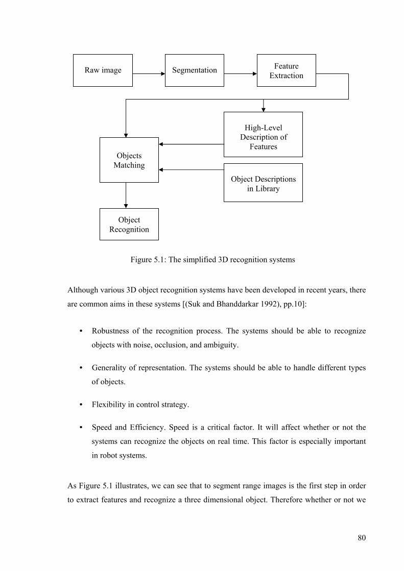
80
Figure 5.1: The simplified 3D recognition systems
Although various 3D object recognition systems have been developed in recent years, there
are common aims in these systems [(Suk and Bhanddarkar 1992), pp.10]:
• Robustness of the recognition process. The systems should be able to recognize
objects with noise, occlusion, and ambiguity.
• Generality of representation. The systems should be able to handle different types
of objects.
• Flexibility in control strategy.
• Speed and Efficiency. Speed is a critical factor. It will affect whether or not the
systems can recognize the objects on real time. This factor is especially important
in robot systems.
As Figure 5.1 illustrates, we can see that to segment range images is the first step in order
to extract features and recognize a three dimensional object. Therefore whether or not we
Raw image Segmentation Feature Extraction
Objects Matching
High-Level Description of
Features
Object Descriptions in Library
Object Recognition

81
can correctly segment the range images is an important factor that affects the recognition
of a three-dimensional object.
Image segmentation is to segment the image into some meaningful non-overlapping
homogeneous regions whose union is the entire image. If we let R be the whole image, R1,
R2 ,…, Rn be the segmented regions, then, according to Gonzalez [(Gonzalez. and Woods.
1992), pp.458], segmentation of an image can be described as follows:
1. RRini ==1∪
2. Ri is a connected region for all i=1,2,…,n.
3. Φ=ji RR ∩ when ji ≠
4. P(Ri)=TRUE for all i=1,2,….,n
5. )( ji RRP ∪ =FALSE when ji ≠
where Φ is the null set and P(Ri) is the logical judge over the points in the set Ri.
There has been general agreement on what results an image segmentation system should
achieve [(Haralick and Shapiro 1992), pp.509]:
• The segmented regions of an image should be uniform and homogeneous
considering some characteristic, e.g., models of the objects in the image.
• Region interiors should contain as less holes as possible.
• Boundaries of regions should be smooth and accurate.
It is very difficult to achieve all these properties at the same time by one segmentation
method. To evaluate the performance of a method for image segmentation, Hoover
suggested to use following five types of metrics (Hoover, Jean-Baptiste et al. 1996):

82
1. Correct detection. If there are more than T percent of the pixels in the segmented
region correctly assigned, the region is correctly detected.
2. Over segmentation. If there are more than T percent of the pixels in a segmented
region that should be assigned to other regions, the detected region is called over
segmented.
3. Under segmentation. If a segmented region contains more than one surface, (which
should be assigned to different regions,) the detected region is called under
segmented.
4. Missing a region. If a region is not contained in any region of correct detection,
over segmentation, or under segmentation in the segmented image, the region is
missed.
5. Noisy region. If a region in the segmented image does not belong to any region of
correct detection, over segmentation, or under segmentation, it is classified as
noise.
where T is a threshold and can be specified by user according to the accuracy requirement
of a system.
There are many three-dimensional image segmentation methods published in the literature.
Generally speaking, these segmentation methods can be classified into two major classes:
1. Edge-based segmentation techniques (Ghosal and Mehrotra 1994; Wani and
Batchelor 1994).
2. Region-based segmentation techniques or clustering techniques (Hoffman and Jain
1987; Jiang and Bunke 1994; Fitzgibbon, Eggert et al. 1995).
In edge-based segmentation methods, it is important to correctly extract the
discontinuities—surface discontinuities (boundaries and jumps) and orientation
discontinuities (creases and roofs), which will be used to guide the followed segmentation
process. The main difficulties that edge-based segmentation techniques meet are:

83
• The effectiveness of these methods will be greatly reduced when range images
contain noise;
• When the edge operator mask size is increased, the computational time will be
greatly increased.
• When the edge pixels detected by edge operator are not continuous (especially in
noisy image), it will be difficult to link these discontinuous pixels.
• Also, the reliability of the crease edge detectors makes edge-based methods
questionable.
Region-based techniques have wider popularity than edge-based techniques. The
essence of region growing techniques is that it segments range images based on the
similarities of feature vectors corresponding to pixels in range images. The region-based
techniques first estimate the feature vectors at each pixel, and then aggregate the pixels
that have similar feature vectors; and at the same time, separate the pixels whose feature
vectors are dissimilar, to form a segmented region.
However, region-based methods also have some problems:
• They have many parameters to control the processing of the region growing.
Most of these parameters need to be predetermined.
• The choice of initial region greatly affects the performance of most region-based
methods. When the seeds are placed on a boundary or on a noise corrupted part of
the image, the results will break down.
• The region boundaries are often distorted because of the noise in the range
images.
• In clustering-based methods, to adaptively estimate the actual number of clusters
in the range image is difficult.
Another way of classifying a segmentation approach is that which uses the notion of
model-driven (top-down). The model-driven methods are appealing because it has been
proved that these methods have similarities to the human cognitive process (Neisser 1967;

84
Gregory 1970). The model-based methods can directly extract the required primitives from
the unprocessed raw range images. Model-based methods, in particular, robust model
based approaches, have been attracting more and more attention (Roth and Levine 1990;
Yu, Bui et al. 1994; Stewart 1995; Miller and Stewart 1996; Lee, Meer et al. 1998). These
methods are very robust to noisy or occluded data.
Next, we will review several state-of-the-art methods of segmentation in section 5.2. Then
we modify the MDPE to produce a quicker version, called QMDPE (Quick-MDPE), and
evaluate its achievements in section 5.3. In section 5.4, we present a model-based method
based on the QMDPE for segmentation of rage images. The performance of the proposed
method is compared to that of several other state-of-the-art range image segmentation
methods in section 5.5. We conclude in section 5.6.
5.2 A Review of Several State-of-the-Art Methods for Range
Image Segmentation
In this section, four methods (UB, UE, USF, WSU) will be reviewed. The USF (Hoover,
Jean-Baptiste et al. 1996) and UE (Fitzgibbon, Eggert et al. 1995) algorithms segment
range images by iteratively growing regions from seed regions. However, the WSU
(Hoffman and Jain 1987; Flynn and Jain 1991) algorithm employs a clustering technique in
its segmentation process. The UB (Jiang and Bunke 1994) algorithm is in region growing
framework, but it is based on straight-line segmentation in scan lines. Next the four
methods will be reviewed in detail.
5.2.1 The USF Range Segmentation Algorithm
The USF algorithm (Hoover, Jean-Baptiste et al. 1996) can be described as follows:
1. Compute the normal of each range pixel.
First, a growing operation is carried out in a n-by-n window from the pixel of
interest. The distances between the pixels (to grow) and their four-connected pixels

85
must be less than a threshold; otherwise, the pixels will be ignored. The normal is
found by either an Eigen method (Duda and Hart 1973; Goldgof, Huang et al.
1989) or a method solving a set of nine plane equations.
2. Choose the seed points.
The pixel with smallest interior measure, corresponding to the residual error of the
plane equation fit to the entire n-by-n window, is chosen as a seed point.
3. Using the seed point to grow the region.
Four criteria for pixels joining the region must be satisfied:
(a) The point is connected to the region grown so far.
(b) Angle between normal of pixel and that of region grown so far is less than a
threshold T1.
(c) Perpendicular distance between pixel and plane grown so far is within a
threshold T2.
(d) Distance of pixel and four-connected neighbor already in the grown region
is less than a threshold T3.
The region is recursively grown until no pixel left to join that region. Then a new region
begins to grow from the next seed point available. If a region’s final size is less than a
threshold T4, the region and its pixels are ignored and will be dealt with during the post-
process step.
5.2.2 The WSU Range Segmentation Algorithm
The WSU algorithm is first presented by Hoffman and Jain (Hoffman and Jain 1987).
Flynn and Jain improved the WSU algorithm and applied it to 3D object recognition
(Flynn and Jain 1991). WSU can be used not only for planar surfaces but also for quadric
surfaces. The details of the WSU algorithm can be described as follows:

86
1 Labelling the jump edge pixels. The distances (dj, j=1,2,…,8) in z between a range
pixel and its eight neighbouring pixels are measured. If dj for all eight points is
greater than a predetermined threshold, the pixel is labelled as a jump edge pixel.
2 Estimating the surface normal of each range pixel. The surface normal of each
range pixel is estimated using k-by-k neighbouring points (but not including jump
edge pixels). A principal component technique (Flynn and Jain 1988) is employed
to estimate the surface normal because this technique can accommodate data
contaminated with noise.
3 Sampling on a regular grid is performed to yield a data set less than 1000 in size.
The normal information and position information of each sampled data point is
used to form six vectors. Then a clustering algorithm (Jain and Dubes 1988) is
employed in the six dimensional space (corresponding to the six vectors).
4 Assigning the range pixels to clusters. Each range pixel is assigned to the
corresponding closest cluster center. The connected component algorithm is used to
avoid assigning the same labels to regions that are not connected.
5 An edge-based merge step is performed. This step will merge the regions where the
average angle between the surface normals of range pixels on one side of the edge
and their neighbours on the other side is less than a predetermined threshold.
6 A principal component procedure is performed to distinguish planar regions from
non-planar regions. The non-planar regions will be ignored in further processing.
7 If regions have similar parameters and are adjacent, they will be merged.
8 Unlabeled pixels on each segment are merged into the region.
9 Step 6, 7 and 8 are repeated until the result does not change.
5.2.3 The UB Range Segmentation Algorithm
The UB segmentation method was developed based on the observation that if a line is used
to scan the image, the points that belong to a planar surface will form a straight line
segment. On the other hand, if the points are on the same straight line segment, they will

87
surely belong to the same planar surface. Unlike other region growing algorithms which
use seeds to grow the regions, the UB segmenter uses straight line segments as growing
primitives. This greatly reduces the data dimension to be dealt with in the growing process
and makes the algorithm very fast.
The UB algorithm can be described as follows (Jiang and Bunke 1994):
1. A median filter is employed as a preprocessing step to reduce the noise level of an
image.
2. Scan the image by scan line and divide the data on each scan line into straight line
segments.
3. Using a link-based data structure, find the neighborhood of each line segment.
4. Select the best seed region by the following process. First choose a small number of
neighboring line segments (three in (Jiang and Bunke 1994)) in a seed region. If
any line segment is shorter than a predetermined threshold, this candidate region is
discarded. The optimal seed region is the one with the smallest error among the
errors computed by a least square plane fitting for each candidature.
5. The growing process is performed. In the UB algorithm, the initial guess is a set of
line segments. A line segment is added to the region if the perpendicular distance
between its two end points and the plane of the region is within a threshold. This
process is continued until no more line segments can be added to this region.
6. The process of seed region finding (step 4) and region growing (step 5) is iterated
until no seed region can be found.
7. A post-processing step is applied to yield clean edges between regions.
5.2.4 The UE Range Segmentation Algorithm
The UE algorithm (Fitzgibbon, Eggert et al. 1995) is similar to the USF algorithm. They
both belong to the class of region growing algorithms. The UE algorithm contains the
following main steps:

88
1. Normal Calculation.
A 5-by-5 window is used to estimate the normal of each range pixel. A normal and
a depth discontinuity are detected using a predetermined normal threshold and
depth threshold.
2. A discontinuity preserving smoothing is performed with multiple passes for greater
smoothing.
3. H-K based segmentation for initialization.
The Gaussian (H) and mean (K) curvature of each pixel is estimated. Using the
combined signs of the pair (H, K), one can judge the surface type of each range
pixel. Each pixel and its eight-connected pixels of similar labeling are grouped to
form initial regions. Then dilation and erosion are performed to fill small unknown
areas and remove small regions.
4. Region growing.
A least squares surface fitting procedure is performed in the initial regions obtained
above. Then each region is in turn grown. To join the region, a point needs to
satisfy the following requirements:
(a) The point is eight-connected to the region grown so far.
(b) The perpendicular distance between the pixel and plane grown so far is
within a threshold.
(c) The angle between normal of the pixel and that of region grown so far is
less than a threshold.
(d) The point is closer to the current surface than any other possible surfaces it
may be assigned to.
(e) The normal of the pixel is in better agreement with the current surface than
any other possible surface it may be assigned to.
After expansion, the surface is refitted using these new points. Then a contraction
of the region boundary is performed.

89
5. Region boundary refinement.
A pixel is added to a region during expansion if:
(a) The point is eight-connected to the region grown so far.
(b) The point-to-plane distance is less than a threshold.
(c) The point is on the one side of a decision surface.
5.2.5 Towards to Model-Based Range Image Segmentation Method
Although the edge-based methods and region-based methods are popular in the computer
vision community, it is difficult for these methods to directly extract specified primitives.
The model-driven (top-down) methods are appealing because they can directly extract the
required primitives from the unprocessed raw range images. The features that are used in
model-driven methods are primitives. So the matching takes place very early in the
recognition process. In the model-based methods, primitive geometric features are matched
instead of similar features that are used in region-based methods. Then matches are
checked for local consistency by using some geometric constraints, e.g. distance, normal,
etc. Because of the introduction of robust statistics into some model-based methods, the
model-based segmentation methods are very robust to noisy or occluded data.
Next, we will present an efficient model-based method for range image segmentation.
5.3 A Quick Version of the MDPE—QMDPE
As shown in chapter 4, MDPE has a very high robustness and can tolerate a large
percentage of outliers including gross noise and pseudo-outliers. However, the time needed
to calculate the densities f (Xi) of all data points within the converged window Wc is large
when the number of the data points is very large. It takes O(n) time to calculate the density
f (Xi) at one point Xi. If there are nw data points within the converged window Wc, the
time complexity of computing the probability density power function ψDP is O(n*nw). In

90
range image processing, nw may be tens of thousands to hundreds of thousands in size. For
such a huge number of range data points, MDPE is not computationally efficient. A
quicker version of MDPE with a similar higher breakdown point to outliers is needed for
range image segmentation.
In this section, we will modify our MDPE to produce a quicker version, called QMDPE.
5.3.1 QMDPE
MDPE measures the entire probability densities of all data points within the converged
mean shift window. However, QMDPE uses only the density of the point in the center of
the converged window. QMDPE, like MDPE, also assumes inliers occupy a relative
majority, with Gaussian-like distribution, of the data points. Thus, when a model to fit is
correctly estimated, the center of the converged window (Xc) in residual space should be as
close to zero as possible; and the probability density f (Xc) of the point at Xc should be as
high as possible. Thus we define the probability density power function, which uses only
one point’s probability density, as follows:
( ))exp(
)(ˆ
XcXcf
DP
α
ψ = ( 5.1)
where α is a factor that adjusts the relative influence of the probability density to the
residual of the point corresponding to the center of the converged window. It is empirically
determined to get the best performance. We adjusted the value of α by comparing the
results in both synthetic data and real image data used in section 4.4, and set it to be 2.0 for
optimal achievement (we note that the empirically best value of α in equation ( 5.1) for
QMDPE is different to that in equation ( 4.7) for MDPE, where α is set to 1.0).
Because only the probability density on the point corresponding to the center of the
converged window needs to be calculated, the time cost to compute the probability density
power in QMDPE is greatly reduced when the number of data is very large (for example,
range image data).
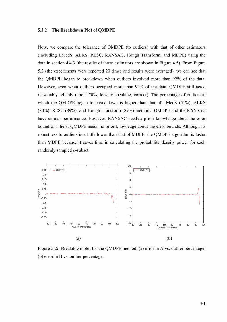
91
5.3.2 The Breakdown Plot of QMDPE
Now, we compare the tolerance of QMDPE (to outliers) with that of other estimators
(including LMedS, ALKS, RESC, RANSAC, Hough Transform, and MDPE) using the
data in section 4.4.3 (the results of those estimators are shown in Figure 4.5). From Figure
5.2 (the experiments were repeated 20 times and results were averaged), we can see that
the QMDPE began to breakdown when outliers involved more than 92% of the data.
However, even when outliers occupied more than 92% of the data, QMDPE still acted
reasonably reliably (about 70%, loosely speaking, correct). The percentage of outliers at
which the QMDPE began to break down is higher than that of LMedS (51%), ALKS
(80%), RESC (89%), and Hough Transform (89%) methods; QMDPE and the RANSAC
have similar performance. However, RANSAC needs a priori knowledge about the error
bound of inliers; QMDPE needs no prior knowledge about the error bounds. Although its
robustness to outliers is a little lower than that of MDPE, the QMDPE algorithm is faster
than MDPE because it saves time in calculating the probability density power for each
randomly sampled p-subset.
(a) (b)
Figure 5.2: Breakdown plot for the QMDPE method: (a) error in A vs. outlier percentage;
(b) error in B vs. outlier percentage.
10 20 30 40 50 60 70 80 90 100
-0.25 -0.2
-0.15 -0.1
-0.05 0
0.05 0.1
0.15 0.2
0.25
Outliers Percentage
Erro
r in
A
QMDPE
10 20 30 40 50 60 70 80 90 100-20
-15
-10
-5
0
5
10
15
20
Outliers Percentage
Erro
r in
B
QMDPE
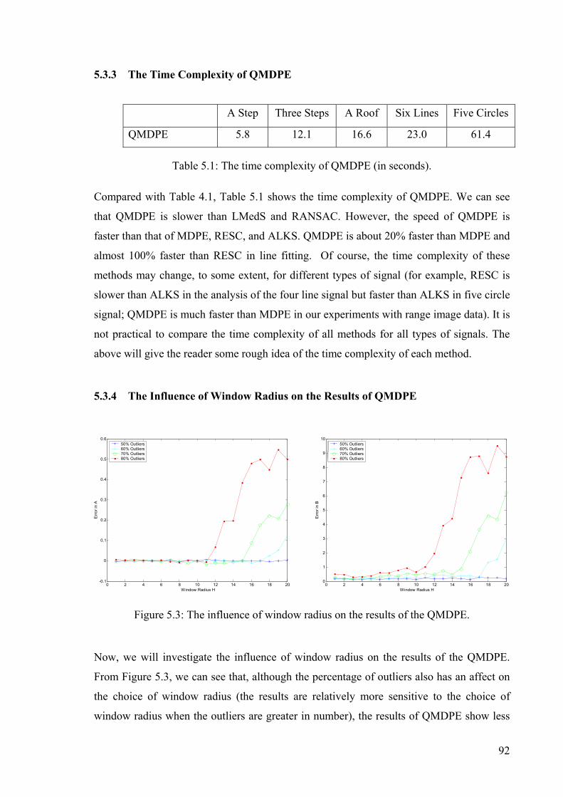
92
5.3.3 The Time Complexity of QMDPE
A Step Three Steps A Roof Six Lines Five Circles
QMDPE 5.8 12.1 16.6 23.0 61.4
Table 5.1: The time complexity of QMDPE (in seconds).
Compared with Table 4.1, Table 5.1 shows the time complexity of QMDPE. We can see
that QMDPE is slower than LMedS and RANSAC. However, the speed of QMDPE is
faster than that of MDPE, RESC, and ALKS. QMDPE is about 20% faster than MDPE and
almost 100% faster than RESC in line fitting. Of course, the time complexity of these
methods may change, to some extent, for different types of signal (for example, RESC is
slower than ALKS in the analysis of the four line signal but faster than ALKS in five circle
signal; QMDPE is much faster than MDPE in our experiments with range image data). It is
not practical to compare the time complexity of all methods for all types of signals. The
above will give the reader some rough idea of the time complexity of each method.
5.3.4 The Influence of Window Radius on the Results of QMDPE
Figure 5.3: The influence of window radius on the results of the QMDPE.
Now, we will investigate the influence of window radius on the results of the QMDPE.
From Figure 5.3, we can see that, although the percentage of outliers also has an affect on
the choice of window radius (the results are relatively more sensitive to the choice of
window radius when the outliers are greater in number), the results of QMDPE show less
0 2 4 6 8 10 12 14 16 18 20-0.1
0
0.1
0.2
0.3
0.4
0.5
0.6
Window Radius H
Erro
r in
A
50% Outliers 60% Outliers 70% Outliers 80% Outliers
0 2 4 6 8 10 12 14 16 18 200
1
2
3
4
5
6
7
8
9
10
Window Radius H
Erro
r in
B
50% Outliers60% Outliers70% Outliers80% Outliers

93
sensitivity to the choice of window radius h than the results of MDPE (see Figure 4.6). The
reason is: the window radius h plays two roles in MDPE. First, h is related to the density
estimation; Second, the density power in MDPE will count all points’ densities within the
converged window (where h is the radius of the window). However, because we use only
one point to estimate the density power, h is only used for density estimation in QMDPE.
5.4 Applying QMDPE to Range Image Segmentation
A good estimator is generally only one component of a complete scheme to successfully
tackle meaningful computer vision tasks. Segmentation requires more than a simple-
minded application of an estimator, no matter how good that estimator is. Several
difficulties faced with applying a statistical estimator to this task must be considered in
designing a method for segmentation.
5.4.1 From Estimator to Segmenter
To test the utility of QMDPE, we apply it to range image segmentation. The range images
were generated by using an ABW structured light scanner and all ABW range images have
512x512 pixels. These ABW range images can be obtained from the USF database
(available at http://marathon.csee.usf.edu/seg-comp/SegComp.html).
However, segmentation is a (surprisingly) complex task and an estimator cannot simply be
directly applied without considering the following factors:
1. The computational cost.
QMDPE is an improved (in speed) MDPE. Its computational cost is much less than
MDPE’s computational cost. Even so, for a range image with a large number of
data points (262,144 data points in our case), employing a hierarchical structure in
our algorithm greatly optimizes the computational speed.
2. Handling of intersections of surfaces.

94
When two surfaces intersect, points around the intersection line may possibly be
assigned to either surface (see Figure 5.5). In fact, the intersection line is on both
surfaces and the data points are inliers to both surfaces. Additional information
(such as the normal to the surface at each pixel) should be used to handle data near
the intersection line.
3. Handling virtual intersection.
It is popular in model-based methods to directly estimate parameters of a primitive;
and classify data points belonging to the primitive according to the estimated
parameters. The data points on the surface will then be masked out and not be
processed in later steps. However, sometimes two surfaces do not actually intersect,
but the extension of one surface is intersected by the other surface. In this case, the
connected component algorithm (Lumia, Shapiro et al. 1983) should be employed.
4. Removal of the isolated outliers.
When all surfaces are estimated, some isolated outliers, due to the noise introduced
by range image camera, may remain. At this stage, a post processing procedure
should be made to eliminate the isolated outliers.
The originators of other novel estimators (e.g. ALKS, RESC, MUSE, MINPRAN) have
also applied their estimators to range image segmentation, but they have not generally
tackled all of the above issues. Hence, even those interested in applying ALKS/RESC, or
any other estimator, to range image segmentation may find several of the components of
our complete implementation independently useful.
5.4.2 A New and Efficient Model-Based Algorithm for Range Image Segmentation
Shadow pixels may occur in an ABW range image. These points cannot give range
information and thus will not be processed.
There are four levels in the hierarchy we used in our algorithm. The bottom level of the
hierarchy contains 64x64 pixels that are obtained by using regular sampling on the original
image. The top level (i=4) of the hierarchy is the original image (512x512). The level i=2
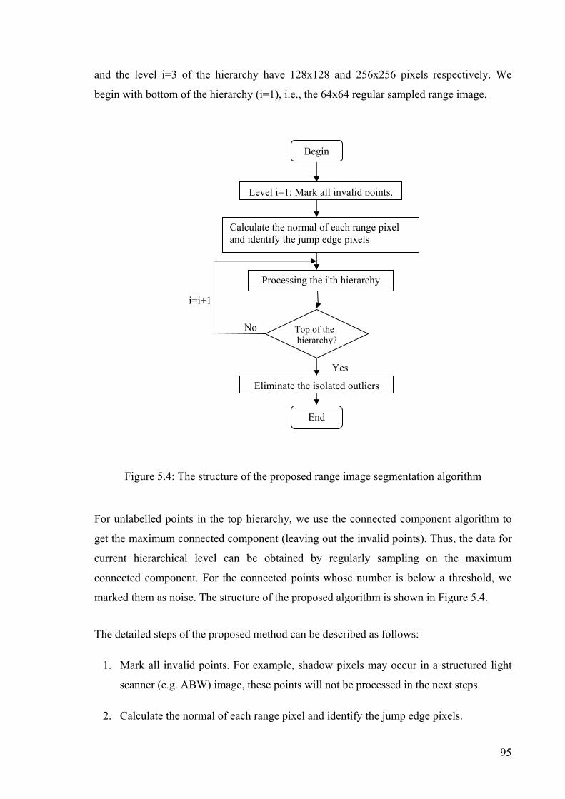
95
and the level i=3 of the hierarchy have 128x128 and 256x256 pixels respectively. We
begin with bottom of the hierarchy (i=1), i.e., the 64x64 regular sampled range image.
Figure 5.4: The structure of the proposed range image segmentation algorithm
For unlabelled points in the top hierarchy, we use the connected component algorithm to
get the maximum connected component (leaving out the invalid points). Thus, the data for
current hierarchical level can be obtained by regularly sampling on the maximum
connected component. For the connected points whose number is below a threshold, we
marked them as noise. The structure of the proposed algorithm is shown in Figure 5.4.
The detailed steps of the proposed method can be described as follows:
1. Mark all invalid points. For example, shadow pixels may occur in a structured light
scanner (e.g. ABW) image, these points will not be processed in the next steps.
2. Calculate the normal of each range pixel and identify the jump edge pixels.
Level i=1; Mark all invalid points.
Calculate the normal of each range pixel and identify the jump edge pixels
Begin
Top of the hierarchy?
Eliminate the isolated outliers
End
Yes
Processing the i'th hierarchy
No
i=i+1

96
Although the QMDPE algorithm was designed to fit the data despite noise and
multiple structures, it requires that the data points of the model should occupy a
relative majority of the whole data. This can be satisfied in a lot of range images (and
the presented algorithm can deal with the whole image as raw image). However, for
some very complicated range images (those with many objects and surfaces), this
requirement is not always satisfied. Using the information provided by the jump edge
will help to coarsely segment the range image to some small regions (each may
include several planes).
3. Employ a hierarchal sampling technique.
The proposed algorithm employs a hierarchal structure based on the fact that when an
image is regularly sampled, the main details will remain while some minor details
may be lost.
4. Apply the QMDPE to obtain the parameters of the estimated primitive.
For the current level in the hierarchy, we use the whole sampled image as the data to
deal with. We apply the QMDPE algorithm to that data which yields the plane
parameters. The inliers corresponding to the estimated plane parameters are then
identified by employing an auxiliary scale estimator. (For historical reason, we
employed a revised Median scale estimator: βα +−
+= )()3
51( 2ii
rmedn
s , where α
and β were experimentally set as 1.8 and 0.2 for optimum. However, an improved
robust scale estimator TSSE (see chapter 7), can be used to estimate the scale of
inliers).
At this stage, it is difficult to tell which plane, of any two intersecting planes, the data
that are on or near the intersection line belong to. Note: this case is not considered in
the popular range image segmentation methods employing robust estimators such as
RESC, MUSE and ALKS. We handle this case in the next step.
5. Using normal information.
When the angle between the normal of the data point that has been classified as an
inlier, and the estimated plane normal, is less than a threshold value (T-angle, 40
degree in our case), the data point is accepted for step 5. Otherwise, the data point is

97
rejected and is classified as a “left-over point” for further processing. As shown in
Figure 5.5, when we did not consider the normal information, the range image was
over segmented because of the intersection of two planes (pointed out by the arrow in
Figure 5.5 (b) and (c)). As comparison, we obtain the right result when we
considered the normal information (see Figure 5.5 (d) and (e)).
6. Using the connected component algorithm to extract the maximum connected
component and label them.
The remaining unlabeled inliers will be used in the next loop for further processing.
7. Select the connected component for processing in the next loop.
For all unlabeled data points, we use jump edge information and connected
component analysis to extract the component with the maximum number of the
connected data points for the next loop. When the number of the data points
belonging to the maximum connected component is larger than a threshold (T-cc), we
repeat step 4-6. Otherwise, we stop this hierarchy and go to the next higher level in
the hierarchy until the top of the hierarchy (512-by-512).
8. Finally, we eliminate the isolated outliers and assign them to the majority of their
eight-connected neighbors.
Compared with current popular methods (region-based and edge-based methods), our
proposed method is a model-based top-down technique. Our method directly extracts the
required primitives from the raw images, and it deals with the whole image as raw image.
Our method is very robust to noisy or occluded data due to the adoption of robust estimator
QMDPE. Because we adopt hierarchical technique, this makes the proposed method
computationally efficient and makes it possible to deal with large size range images with
only small extra computational cost.

98
(a) (b) (c)
(d) (e) (f)
Figure 5.5: A comparison of using normal information or not using normal information. (a)
Range image (ABW test.10 from the USF database); (b) The segmentation result without
using normal information; (c) The points near or on the intersection of two planes may be
classified to both planes without considering normal information; (d, e) The result using
normal information; (f) The ground truth result.
5.5 Experiments in Range Image Segmentation
In this section, we will show how to use our method to segment range images. Since one
main advantage of our method, over the traditional methods, is that it can resist the
influence of noise, we put some randomly distributed noise into the range images (Note, as
the whole image is dealt with at the beginning of the segmentation, there is also a high
percentage of pseudo-outliers existing in the data).
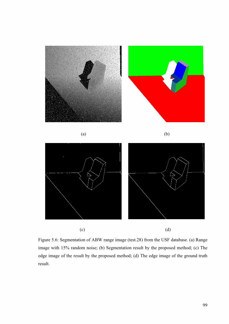
99
(a) (b)
(c) (d)
Figure 5.6: Segmentation of ABW range image (test.28) from the USF database. (a) Range
image with 15% random noise; (b) Segmentation result by the proposed method; (c) The
edge image of the result by the proposed method; (d) The edge image of the ground truth
result.

100
(a) (b)
(c) (d)
Figure 5.7: Segmentation of ABW range image (test.27) from the USF database. (a) Range
image with 15% random noise; (b) Segmentation result by the proposed method; (c) The
edge image of the result by the proposed method; (d) The edge image of the ground truth
result.

101
(a) (b)
(c) (d)
Figure 5.8: Segmentation of ABW range image (test.13) from the USF database. (a) Range
image with 15% random noise; (b) Segmentation result by the proposed method; (c) The
edge image of the result by the proposed method; (d) The edge image of the ground truth
result.

102
In Figure 5.6, Figure 5.7, and Figure 5.8 (a), we add 15% randomly distributed noise, i.e.
39322 noisy points were added to each range image taken from the USF ABW range
image database (test28, test27, and test13). As shown Figure 5.6, Figure 5.7, and Figure
5.8 (b) and (c), our method can resist the influence of large number of noise corrupted
points. The main surfaces were recovered by our proposed method. Only a slight distortion
appeared on some boundaries of neighbouring surfaces. In fact, the accuracy of the range
data, and the accuracy of normal at each range point, will have an effect on the distortion.
It is important to compare the results of our method with the results of other methods. We
also compare our results with those of the three state-of-art range image segmenters (i.e.
the USF, WSU and UB, see (Hoover, Jean-Baptiste et al. 1996)).
(a) (b) (c)
(d) (e) (f)
Figure 5.9: Comparison of the segmentation results for ABW range image (test.1) from the
USF database. (a) Range image; (b) The result of ground truth; (c) The result by the USF;
(d) The result by the WSU; (e) The result by the UB; (f) The result by the proposed
method.
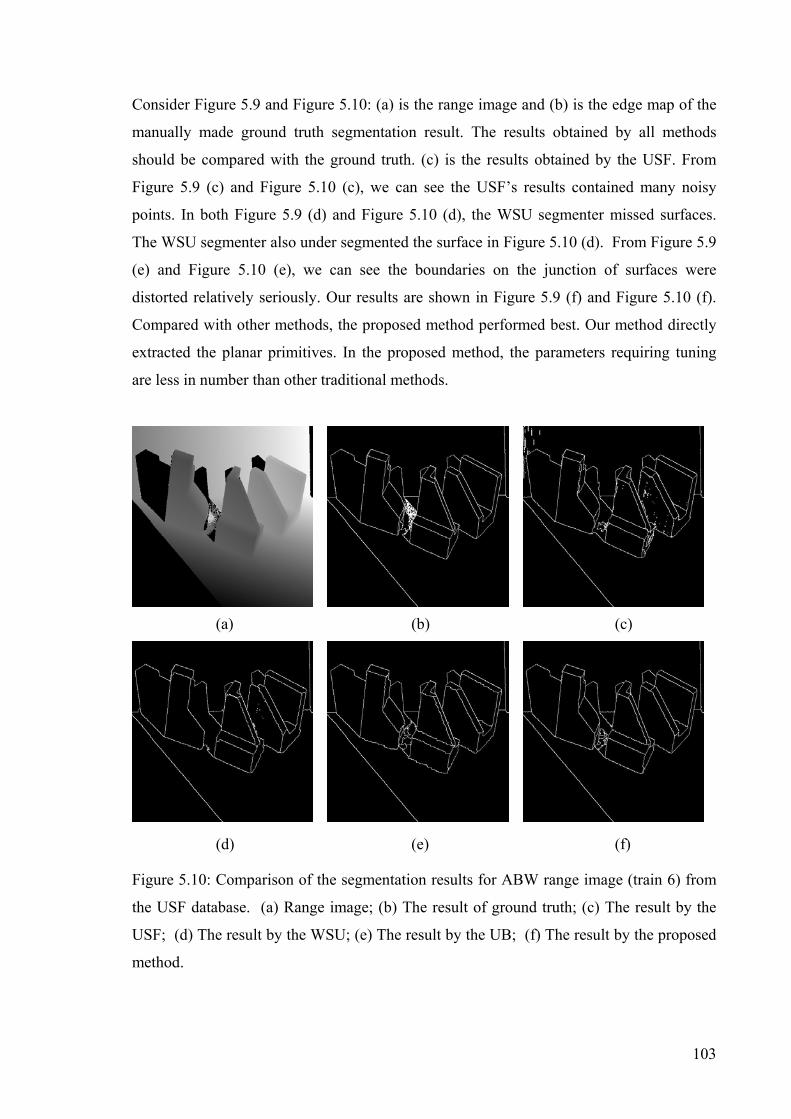
103
Consider Figure 5.9 and Figure 5.10: (a) is the range image and (b) is the edge map of the
manually made ground truth segmentation result. The results obtained by all methods
should be compared with the ground truth. (c) is the results obtained by the USF. From
Figure 5.9 (c) and Figure 5.10 (c), we can see the USF’s results contained many noisy
points. In both Figure 5.9 (d) and Figure 5.10 (d), the WSU segmenter missed surfaces.
The WSU segmenter also under segmented the surface in Figure 5.10 (d). From Figure 5.9
(e) and Figure 5.10 (e), we can see the boundaries on the junction of surfaces were
distorted relatively seriously. Our results are shown in Figure 5.9 (f) and Figure 5.10 (f).
Compared with other methods, the proposed method performed best. Our method directly
extracted the planar primitives. In the proposed method, the parameters requiring tuning
are less in number than other traditional methods.
(a) (b) (c)
(d) (e) (f)
Figure 5.10: Comparison of the segmentation results for ABW range image (train 6) from
the USF database. (a) Range image; (b) The result of ground truth; (c) The result by the
USF; (d) The result by the WSU; (e) The result by the UB; (f) The result by the proposed
method.

104
As stated before, adopting hierarchical sampling technique in the proposed method greatly
reduces its time cost. The processing time of the method is affected to a relatively large
extent by the number of surfaces in the range images. The processing time for a range
image including simple objects is faster than that for a range image including complicated
objects. Generally speaking, it takes about 40 seconds (on an AMD800MHz personal
computer programmed (un-optimized) in the C language) for segmenting a range image
with less surfaces and about 80-100 seconds for a range image including more surfaces.
This includes the time for computing normal information at each range pixel (which takes
about 12 seconds).
5.6 Conclusion
In this chapter, we developed a quicker version of MDPE called QMDPE. The advantage
of QMDPE is that only the probability density corresponding to the center of the
converged mean shift window needs to be calculated; therefore the time cost to compute
the probability density power is greatly reduced. Although QMDPE has a relatively lower
tolerance to outliers than MDPE, QMDPE still has a better tolerance than most available
estimators (such as M-estimators, LMedS, LTS, RANSAC, ALKS, and RESC). We
recommend that when the number of data points are small (say less than 5000 points) and
the task has a high reliance on the robustness of the estimator, MDPE is an ideal choice.
On the other hand, when the task involves a large number of data points (for example,
range image segmentation which often involves more than tens of thousands of data), and
the speed is a relatively important factor to consider, it is better to choose QMDPE rather
than MDPE.
The second contribution of this chapter is that we apply the new QMDPE to the computer
vision task of segmenting range data. This part is more than a mere application of the
estimator in a straightforward manner. There are a number of issues that need to be
addressed when applying an estimator (any estimator) to such a problem. The solutions we
have found, to these practical problems that arise in the segmentation task, should be of
independent interest. The resulting combination of a highly robust estimator and a very

105
careful application of that estimator, produces a very effective method for range
segmentation.
Experimental comparisons of the proposed approach, and several other state-of-the-art
methods, support the claim that the proposed method is more robust to outliers and can
achieve good results even when the range images are contaminated by a large number of
(impulse) noisy data points.
In (Roth and Levine 1990), the authors also employed a robust estimator—LMedS to
segment range image. They firstly found the largest connected region bounded by edge
pixels; then they used LMedS to fit the geometric primitive in the chosen region. They
assumed the largest connected region contained only one geometric primitive. However, if
the region includes more than two geometric primitives (for complicated range images),
and each geometric primitive has less than 50% data in the region, the estimated primitive
will be wrong because LMedS has only up to 0.5 breakdown point.
The algorithm proposed in this chapter is a model-based method and can directly extract
planar primitives from the raw images. Because QMDPE is very robust to noise, the
algorithm has the advantage that it can resist the influence of a large amount of random
noise in the range image. Also, the proposed algorithm is robust to the presence of multiple
structures. Since we sequentially removed the detected surfaces one by one, the average
time to segment the range image will be affected by how many surfaces the range image
includes. However, the computing time will not be greatly affected by the size of the range
image as we use a sampling hierarchical technique.

106
6. Variable-Bandwidth QMDPE for Robust Optical Flow Calculation
6.1 Introduction
One major task of computer vision is to compute the optical flow from image sequences
(Horn and Schunck 1981; Nagel 1987; Fleet and Jepson 1990; Barron, Fleet et al. 1994;
Black 1994; Black and Jepson 1996; Lai and Vemuri 1998; Memin and Perez 1998; Ong
and Spann 1999; Farneback. 2000; Farneback 2001; Memin and Perez 2002). Accurate
computation of optical flow is an important foundation for tasks, such as motion
segmentation, extracting structure from motion, etc. Traditional methods of computing
optical flow are non-robust. Which means that they will fail to correctly compute optical
flow when the two assumptions: data conservation and spatial coherence, are violated.
Clearly, these assumptions will be violated near motion boundaries, and when shadows,
occlusions, and/or transparent motions are present.
During the last ten years, robust techniques, such as: M-estimators (Black and Anandan
1993; Black and Anandan 1996), Least Median Squares (LMedS) estimator (Bab-
Hadiashar and Suter 1998; Ong and Spann 1999), Least Trimmed Squares (LTS)
estimators (Ming and Haralick 2000), and robust Total Least Squares (TLS) estimator
1.1.5. Chapter 6
Variable-Bandwidth QMDPE for Robust Optical Flow Calculation

107
(Bab-Hadiashar and Suter 1998) etc., have been employed to extract optical flow. Because
these robust estimators can tolerate the influence of “bad” data, i.e. outliers, they usually
obtain better results. Unfortunately, these robust estimators have a breakdown point no
more than 50%. This means that when the data contain more than 50% outliers, these
estimators will totally breakdown. Such may happen, for example, near motion boundary.
In this chapter, we will provide, based on our previous work [see (Wang and Suter 2002a;
Wang and Suter 2003b); also see chapter 4 and 5], a robust estimator—variable bandwidth
QMDPE (vbQMDPE). Some others may prefer the term Adaptive-Bandwidth QMDPE—
abQMDPE. Instead of using a fixed bandwidth as in QMDPE, vbQMDPE uses data-driven
bandwidth selection. We apply the novel proposed vbQMDPE to the task of optical flow
computation. We also correct the results of Bab-Hadiashar and Suter (Bab-Hadiashar and
Suter 1998) for the Otte image sequence.
vbQMDPE is very robust if the percentage of outliers is less than 80%, outperforming
most other methods in optical flow computation. Of course, any method can breakdown
under extreme data: even LMedS and LTS can breakdown when clustered outliers are
present - despite those outliers constituting less than 50% of the whole data (e.g., see
section 4.4.2).
6.2 Optical Flow Computation
Let I(x, y, t) be the luminance of a pixel at position (x, y) and time t, and v = (u, v) be the
optical flow. The data conservation assumption implies (Fennema and Thompson 1979):
I(x, y, t)) = I(x + uδt, y + vδt, t + δt) ( 6.1)
First order expansion yields the optical flow constraint (OFC) equation:
0=∂∂+
∂∂+
∂∂
tIv
yIu
xI
( 6.2)
where (∂I/∂x, ∂I/∂y, and ∂I/∂t) are partial derivatives of luminance I with respect to space
and time at point (x, y, t)).
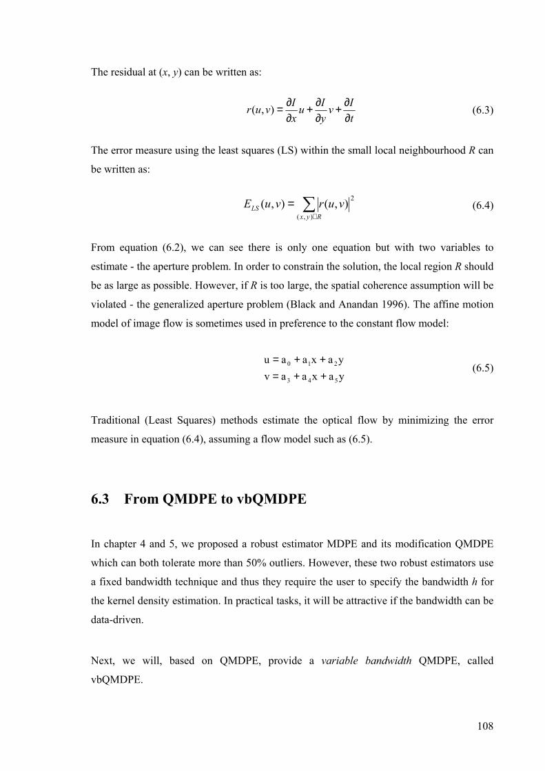
108
The residual at (x, y) can be written as:
tIv
yIu
xIvur
∂∂+
∂∂+
∂∂=),( ( 6.3)
The error measure using the least squares (LS) within the small local neighbourhood R can
be written as:
∑∈
=Ryx
LS vurvuE),(
2),(),( ( 6.4)
From equation ( 6.2), we can see there is only one equation but with two variables to
estimate - the aperture problem. In order to constrain the solution, the local region R should
be as large as possible. However, if R is too large, the spatial coherence assumption will be
violated - the generalized aperture problem (Black and Anandan 1996). The affine motion
model of image flow is sometimes used in preference to the constant flow model:
ya x a avya x a au
543
210
++=++=
( 6.5)
Traditional (Least Squares) methods estimate the optical flow by minimizing the error
measure in equation ( 6.4), assuming a flow model such as ( 6.5).
6.3 From QMDPE to vbQMDPE
In chapter 4 and 5, we proposed a robust estimator MDPE and its modification QMDPE
which can both tolerate more than 50% outliers. However, these two robust estimators use
a fixed bandwidth technique and thus they require the user to specify the bandwidth h for
the kernel density estimation. In practical tasks, it will be attractive if the bandwidth can be
data-driven.
Next, we will, based on QMDPE, provide a variable bandwidth QMDPE, called
vbQMDPE.

109
6.3.1 Bandwidth Choice
One crucial issue in the non-parametric density estimation, and the mean shift method, is
how to choose h (Wand and Jones 1995; Comaniciu, Ramesh et al. 2001; Comaniciu and
Meer 2002a). We employ a method in (Wand and Jones 1995):
snKu
KRh5/1
22 )(35
)(243ˆ
= ( 6.6)
where and . , s is the sample standard deviation.
A robust median scale estimator is then given by (Rousseeuw and Leroy 1987):
s = 1.4826medixi ( 6.7)
h will provide a upwards bound on the AMISE (asymptotic mean integrate error) optimal
bandwidth AMISEh , thus we choose the bandwidth as c h , c is a constant number (0<c<1)
and is used to avoid over-smoothing (we are also aware that if the value of the bandwidth
is too small, it will introduce artefacts).
The median scale estimator in equation ( 6.7) may be biased for non-symmetrical multi-
model data and for data with more than 50% outliers. However, the influence of the
bandwidth h on the final result is relatively weak as it is only used in the pdf estimation
and the mean shift method.
6.3.2 The Algorithm of the Variable Bandwidth QMDPE
The vbQMDPE procedure can be written as follows:
1 Randomly choose one p-subset, estimate the model parameters by the p-subset, and
calculate the residuals of all data points.
2 Adaptively choose the bandwidth h using the method described in section 6.3.1.
∫−=1
1
2)()( ζζ dKKR ∫−=1
1
22 )()( ζζζ dKKu
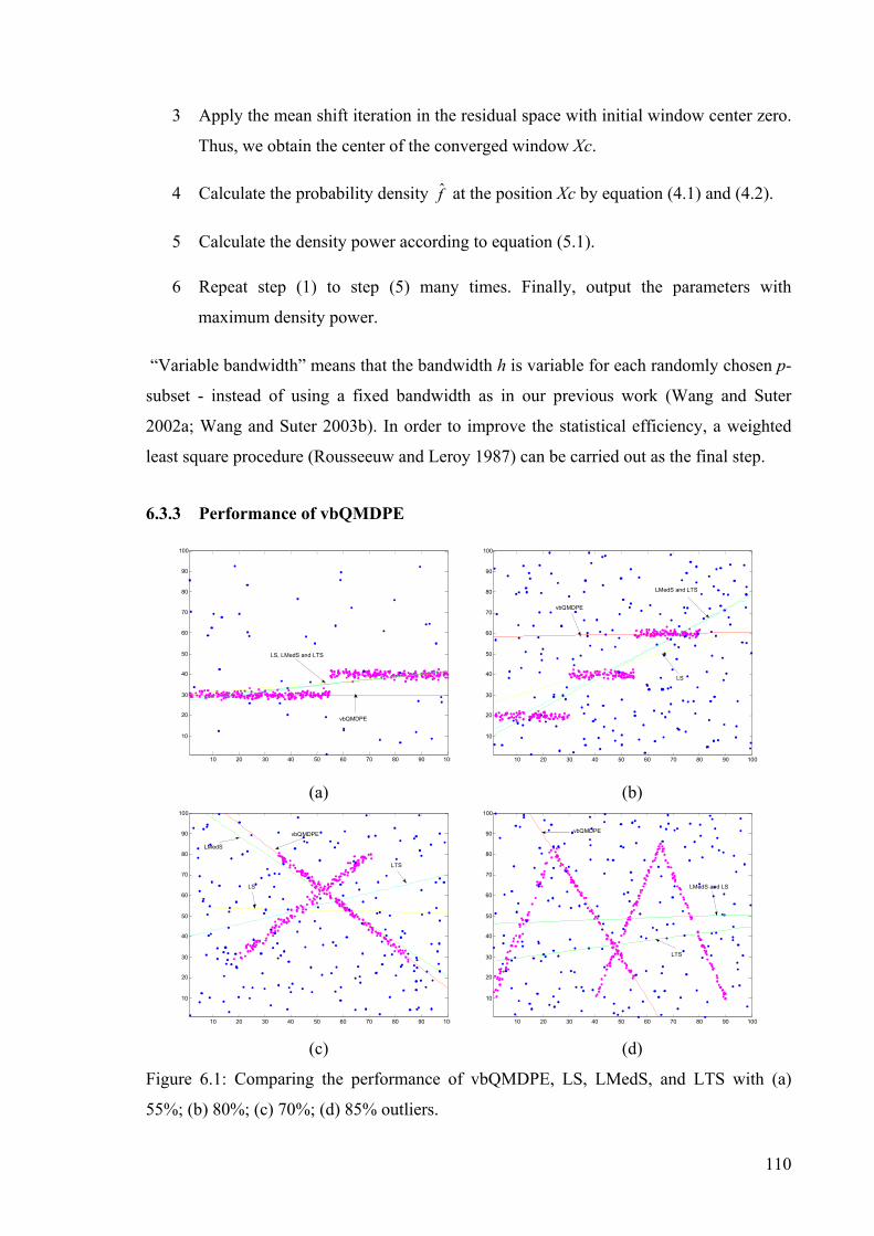
110
10 20 30 40 50 60 70 80 90 100
10 20 30 40 50 60 70 80 90
100
vbQMDPE
LS, LMedS and LTS
10 20 30 40 50 60 70 80 90 100
10
20
30
40
50
60
70
80
90
100
vbQMDPE
LS
LMedS and LTS
10 20 30 40 50 60 70 80 90 100
10 20 30 40 50 60 70 80 90
100 vbQMDPE
LMedS
LS
LTS
10 20 30 40 50 60 70 80 90 100
10
20
30
40
50
60
70
80
90
100
vbQMDPE
LMedS and LS
LTS
3 Apply the mean shift iteration in the residual space with initial window center zero.
Thus, we obtain the center of the converged window Xc.
4 Calculate the probability density f at the position Xc by equation ( 4.1) and ( 4.2).
5 Calculate the density power according to equation ( 5.1).
6 Repeat step (1) to step (5) many times. Finally, output the parameters with
maximum density power.
“Variable bandwidth” means that the bandwidth h is variable for each randomly chosen p-
subset - instead of using a fixed bandwidth as in our previous work (Wang and Suter
2002a; Wang and Suter 2003b). In order to improve the statistical efficiency, a weighted
least square procedure (Rousseeuw and Leroy 1987) can be carried out as the final step.
6.3.3 Performance of vbQMDPE
(a) (b)
(c) (d)
Figure 6.1: Comparing the performance of vbQMDPE, LS, LMedS, and LTS with (a)
55%; (b) 80%; (c) 70%; (d) 85% outliers.

111
We demonstrate that vbQMDPE is very robust to outliers by comparing it to several other
traditional methods (the LS, LMedS and LTS methods, which are frequently employed in
optical flow calculation).
First, we take a simple setting — line fitting. We generated four kinds of data (one step,
two steps, two crossed lines, and four lines), each with a total of 500 data points. The
signals were corrupted by Gaussian noise with zero mean and unit standard variance.
Among the 500 data points, α data points were randomly distributed in the range of (0,
100). The i'th structure has ni data points.
The four signals are as follows:
• One step: x:(0-55), y=30, n1=225; x:(55-100), y=40, n2=225; α=50.
• Two steps: x:(0-30), y=20, n1=100; x:(30-55), y=40, n2=100; x:(55-80), y=60,
n3=100; α=200.
• Two crossed lines: x:(20-70), y=x+10, n1=150; x:(35-85), y=115-x, n2=150; α=200.
• Four lines: x:(0-25), y=3x+10, n1=75; x:(25-55), y=130-2x, n2=20; x:(40-65), y=3x-
110, n3=75; x:(65-90), y=280-3x, n4=75; α=370.
From Figure 6.1, we can see that LS is non-robust, and that LMedS and LTS failed to fit
all the four signals. Only vbQMDPE correctly fitted all the four signals - not even breaking
down when the data includes 85% outliers (Figure 6.1 (d)).
6.4 vbQMDPE and Optical Flow Calculation
The optical flow constraint (OFC) is a linear equation in u-v space. Each pixel gives rise to
one such linear constraint and, in a noise-free setting, and assuming constant u and v, all
lines intersect at a common point.

112
-5 -4 -3 -2 -1 0 1 2 3 4 5-8 -6 -4 -2 0 2 4 6 8
U
V
vbQMDPE
LMedS
LS
LTS
5 10 15 20 25 30
5
10
15
20
25
30
Two main difficulties in optical flow estimation are (Nesi, Del Bimbo et al. 1995):
• The discontinuities in the local velocity;
• The “aperture” problem.
(a) (b)
(c)
Figure 6.2: One example of multiple motions.
The first difficulty is related to occlusions between image illumination discontinuities,
moving objects or moving object boundaries. One solution to the second difficulty is to
enlarge the local window so as to collect more constraint equations to over determine the
optical flow; this will bring higher statistical efficiency. However, enlarging the window

113
means more chance of including multiple motions (forming multiple clusters of
intersecting lines e.g., Figure 6.2). Because traditional estimators (M-estimators, LMedS,
LTS, etc.) have only up to 50% breakdown point, they may fail to compute optical flow
when the data include multiple motion structures (i.e. the outliers occupy more than 50%
of the data). In such cases, vbQMDPE performs well.
We generated an image sequence with two moving squares using the method similar to that
in (Barron, Fleet et al. 1994). Figure 6.2 (a) shows one snapshot of the image sequence.
The correct optical flow is shown in Figure 6.2 (b). The small window centered at (110,
136) in Figure 6.2 (a) includes three motions: each motion involves less than 50% data
points. Its OFC plot, using symbolically determined derivatives of the image intensities I,
is shown in Figure 6.2 (c). From Figure 6.2 (c), we can see that there are three motions
included in the small window in Figure 6.2 (a). The optical flow of each motion (2.0, 1.0),
(-3.0, 1.5), (3.0, -1.5) is marked by a red-plus sign. The proposed robust estimator gives the
correct optical flow estimation (3.0, -1.5). However, by the LMedS method, the estimated
optical flow is (2.36, -0.71); and the estimated optical flow by the least trimmed squares
and the least squares method is respectively (2.71, -1.43) and (0.06, 0.84).
6.4.1 Variable-Bandwidth-QMDPE Optical Flow Computation
The first step to compute optical flow is to estimate the spatio-temporal derivatives of the
image brightness. We follow Bab-Hadiashar and Suter (Bab-Hadiashar and Suter 1998),
and Nagel (Nagel 1995), by convolving the image brightness with derivatives of 3D spatio-
temporal Gaussian function:
( )T 11 x x
23/ 2
1(x)2
G eπ
−− Σ=
Σ ( 6.8)
where x =(x, y, t)T; Σ is the covariance matrix.
There are methods to estimate the derivatives near the discontinuities of optical flow (e.g.,
(Ye and Haralick 2000)). In our simple approach, we first estimate the derivatives of I with
initial standard variance σ0. Then, when the estimated derivatives (Ix, Iy, and It) are larger

114
than a threshold, we simply re-compute the derivatives with half of the standard variance
in that corresponding direction.
For each NxN patch of the image and chosen motion model (in our case, constant motion
model and affine motion model), we solve for the flow using the vbQMDPE. The measure
of reliability in (Bab-Hadiashar and Suter 1998) can be employed in our method.
6.4.2 Quantitative Error Measures for Optical Flow
When the “ground truth” optical flow of image sequences is known, the error analysis is
performed by Barron’s method (Barron, Fleet et al. 1994). The angular error measure is
reported in degree:
E = arcos(ve , vc) ( 6.9)
where ve= 1/)1,,( 22 ++ vuvu T and vc is the true motion vector. The average and standard
deviation of the errors are both reported.
6.5 Experimental Results on Optical Flow Calculation
The proposed algorithm has been evaluated on both synthetic and real images. Three well-
known image sequences (the Diverging Tree sequence (which is obtained from
ftp://csd.uwo.ca/pub/vision); the Yosemite sequence (which is obtained from
ftp://csd.uwo.ca/pub/vision); and the Otte image sequence (which is obtained from
http://i21www.ira.uka.de/image_sequences/)) are used (see Figure 6.3). Table 6.1 shows
the comparison results the Diverging Tree sequence (Figure 6.3 (a)) – showing the
proposed method gives the most accurate results for affine motion model. Even for the
constant motion model, vbQMDPE still yields better results than most other comparative
methods.
Figure 6.3 (b) shows one snapshot of the Yosemite sequence. Because the true motion of
the clouds does not really reflect the image brightness changes, we exclude the clouds in
our experiments. From Table 6.2, we can see that the proposed algorithm and Farneback’s
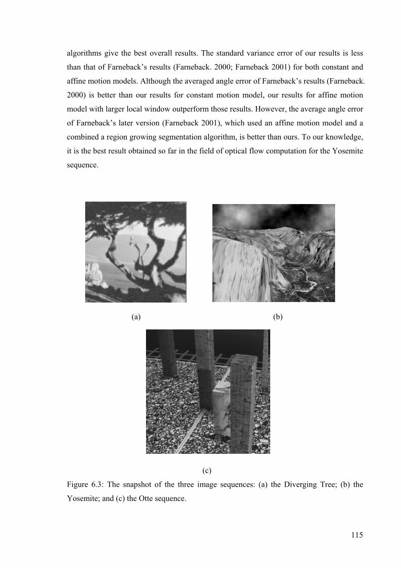
115
algorithms give the best overall results. The standard variance error of our results is less
than that of Farneback’s results (Farneback. 2000; Farneback 2001) for both constant and
affine motion models. Although the averaged angle error of Farneback’s results (Farneback.
2000) is better than our results for constant motion model, our results for affine motion
model with larger local window outperform those results. However, the average angle error
of Farneback’s later version (Farneback 2001), which used an affine motion model and a
combined a region growing segmentation algorithm, is better than ours. To our knowledge,
it is the best result obtained so far in the field of optical flow computation for the Yosemite
sequence.
(a) (b)
(c)
Figure 6.3: The snapshot of the three image sequences: (a) the Diverging Tree; (b) the
Yosemite; and (c) the Otte sequence.
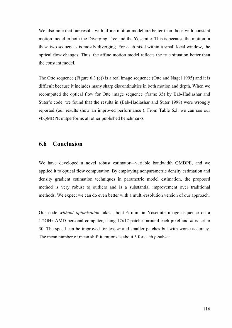
116
We also note that our results with affine motion model are better than those with constant
motion model in both the Diverging Tree and the Yosemite. This is because the motion in
these two sequences is mostly diverging. For each pixel within a small local window, the
optical flow changes. Thus, the affine motion model reflects the true situation better than
the constant model.
The Otte sequence (Figure 6.3 (c)) is a real image sequence (Otte and Nagel 1995) and it is
difficult because it includes many sharp discontinuities in both motion and depth. When we
recomputed the optical flow for Otte image sequence (frame 35) by Bab-Hadiashar and
Suter’s code, we found that the results in (Bab-Hadiashar and Suter 1998) were wrongly
reported (our results show an improved performance!). From Table 6.3, we can see our
vbQMDPE outperforms all other published benchmarks
6.6 Conclusion
We have developed a novel robust estimator—variable bandwidth QMDPE, and we
applied it to optical flow computation. By employing nonparametric density estimation and
density gradient estimation techniques in parametric model estimation, the proposed
method is very robust to outliers and is a substantial improvement over traditional
methods. We expect we can do even better with a multi-resolution version of our approach.
Our code without optimization takes about 6 min on Yosemite image sequence on a
1.2GHz AMD personal computer, using 17x17 patches around each pixel and m is set to
30. The speed can be improved for less m and smaller patches but with worse accuracy.
The mean number of mean shift iterations is about 3 for each p-subset.

117
Table 6.1: Comparative results on diverging tree: the first part of the table is the results
reported by Barron et. al (1994) and Ong et. al (1999); the second part is the results
obtained by the proposed algorithm (number 2 and 6 represent constant and affine motion
models).
Technique Avg. error
(degree)
Std. dev.
(degree)
Density
( % )
Horn and Schunck (original unthresholded)
Horn and Schunck (modified unthresholded)
Uras et.al. (unthresholded)
Nagel
Anandan
Singh (Step 1 unthresholded)
Singh (Step 2 unthresholded)
Least-Squares (block-based) method (in Ong
and Spann, 1999)
12.02
2.55
4.64
2.94
7.64
17.66
8.60
1.98
11.72
3.67
3.48
3.23
4.96
14.25
4.78
2.81
100
100
100
100
100
100
100
100
vbQMDPE2 (σ0=1.5, 11x11, m=30)
vbQMDPE6 (σ0=1.5, 11x11, m=30)
2.51
1.46
1.62
1.03
100
100
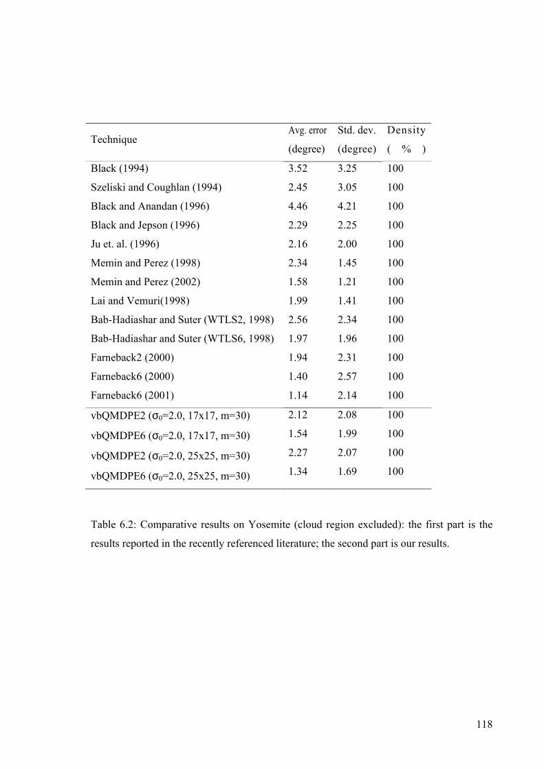
118
Table 6.2: Comparative results on Yosemite (cloud region excluded): the first part is the
results reported in the recently referenced literature; the second part is our results.
Technique Avg. error
(degree)
Std. dev.
(degree)
Density
( % )
Black (1994)
Szeliski and Coughlan (1994)
Black and Anandan (1996)
Black and Jepson (1996)
Ju et. al. (1996)
Memin and Perez (1998)
Memin and Perez (2002)
Lai and Vemuri(1998)
Bab-Hadiashar and Suter (WTLS2, 1998)
Bab-Hadiashar and Suter (WTLS6, 1998)
Farneback2 (2000)
Farneback6 (2000)
Farneback6 (2001)
3.52
2.45
4.46
2.29
2.16
2.34
1.58
1.99
2.56
1.97
1.94
1.40
1.14
3.25
3.05
4.21
2.25
2.00
1.45
1.21
1.41
2.34
1.96
2.31
2.57
2.14
100
100
100
100
100
100
100
100
100
100
100
100
100
vbQMDPE2 (σ0=2.0, 17x17, m=30)
vbQMDPE6 (σ0=2.0, 17x17, m=30)
vbQMDPE2 (σ0=2.0, 25x25, m=30)
vbQMDPE6 (σ0=2.0, 25x25, m=30)
2.12
1.54
2.27
1.34
2.08
1.99
2.07
1.69
100
100
100
100

119
Table 6.3: Comparative results on Otte image sequences: the first part was reported by
Bab-Hadiashar and Suter (1998); the second part is the corrected results; the third part is
obtained by running the proposed algorithm.
Technique Avg. error
(degree)
Std. dev.
(degree)
Density
( % )
Giachetti and Torre (1996)
Bab-Hadiashar and Suter (WLS2, 1998)
Bab-Hadiashar and Suter (WLS6, 1998)
Bab-Hadiashar and Suter (WTLS2, 1998)
Bab-Hadiashar and Suter (WTLS6, 1998)
5.33
3.39
3.51
3.74
3.67
-----
6.55
6.48
8.09
7.37
100
100
100
100
100
Bab-Hadiashar and Suter (WLS2, corrected)
Bab-Hadiashar and Suter (WLS6, corrected)
Bab-Hadiashar and Suter (WTLS2, corrected)
Bab-Hadiashar and Suter (WTLS6, corrected)
3.02
3.14
3.20
3.20
5.98
5.84
7.02
6.59
100
100
100
100
vbQMDPE2 (σ0=2.0, 17x17, m=30)
vbQMDPE6 (σ0=2.0, 17x17, m=30)
vbQMDPE2 (σ0=2.0, 25x25, m=30)
vbQMDPE6 (σ0=2.0, 25x25, m=30)
2.64
2.82
2.21
2.29
4.98
5.03
4.16
4.06
100
100
100
100

120
7. A Highly Robust Scale Estimator for Heavily Contaminated Data
It is not enough to (only) correctly estimate the parameters of a model to differentiate
inliers from outliers; It is also important to robustly estimate the scale of inliers. In this
chapter, we propose a new robust scale estimation technique: robust Two-Step Scale
estimator (TSSE). The TSSE applies nonparametric density estimation and density
gradient estimation techniques, to robustly estimate the scale of inliers for heavily
contaminated data. The TSSE can tolerate more than 80% outliers and comparative
experiments show its advantages over five other robust scale estimators: the median, the
median absolute deviation (MAD), Modified Selective Statistical Estimator (MSSE),
Residual Consensus (RESC), and Adaptive Least Kth order Squares (ALKS).
7.1 Introduction
As emphasized in chapter 2, in computer vision tasks, it frequently happens that gross
noise and pseudo outliers occupy the absolute majority of the data. Most past work aimed
at presenting robust estimators with high breakdown point (Rousseeuw 1984; Yu, Bui et al.
1994; Stewart 1995; Miller and Stewart 1996; Lee, Meer et al. 1998), i.e. the estimator can
1.1.6. Chapter 7
A Highly Robust Scale Estimator for Heavily Contaminated Data
121
correctly find the parameters of a model from the data which are heavily contaminated.
However, correctly estimating the parameters of a model is not enough to differentiate
inliers from outliers. Having a correct scale of inliers is crucial to the robust behaviour of
an estimator. The success of some robust estimators is based on having correct initial scale
estimate, or the correct setting of a particular parameter that is related to scale (e.g.,
RANSAC, Hough Transform, M-estimators etc.). Thus, their performance crucially
depends on that user-provided scale-related knowledge. Robust scale estimation is often
attempted during a post-processing stage of robust estimators (such as LMedS, LTS, etc.).
Yet, although there are a lot of papers that propose robust estimators with high breakdown
point for model fitting, robust scale estimation is relatively neglected.
In this chapter, we investigate the behaviour of several robust scale estimators that are
widely used in computer vision community and show the problems of these scale
estimation techniques. We also propose a new robust scale estimator: Two-Step Scale
estimator (TSSE), based on the nonparametric density estimation and density gradient
estimation techniques. TSSE can tolerate more than 80% outliers and outperform the five
comparative scale estimators (The Median, MAD, ALKS, RESC, MSSE scale estimators).
This chapter is organized as follows: in section 7.2, we review previous robust scale
techniques. In section 7.3, we propose a simple but efficient mean shift valley algorithm,
by which the local valley can be found and propose the novel robust scale estimator: TSSE.
TSSE is experimentally compared with five other robust scale estimators, using data with
multiple structures, in section 7.4. We conclude in section 7.5.
7.2 Robust Scale Estimators
The emphasis in many past computer vision papers presenting robust estimators was on the
high breakdown point (Rousseeuw 1984; Rousseeuw and Leroy 1987; Yu, Bui et al. 1994;
Stewart 1995; Miller and Stewart 1996; Lee, Meer et al. 1998; Wang and Suter 2003b), i.e.
the estimator that can correctly find the parameters of a model from the data which are
heavily contaminated. Whether or not the inliers can be successfully differentiated from
the outliers depends on two factors:

122
(1) Whether the parameters of a model are correctly found; and
(2) Whether the scale of inliers is correctly estimated.
Step (2), scale estimation plays an important role in the overall robust behaviour of these
methods. Some robust estimators, such as M-estimators, RANSAC, Hough Transform,
etc., put the onus on the "user" - they simply require some user-set parameters that are
linked to the scale of inliers. Others, such as LMedS, RESC, MDPE, QMDPE, etc., use an
auxiliary estimate of scale (after finding the parameters of a model) during a post-
processing stage, which aims to differentiate inliers from outliers.
Given a scale estimate, s, the inliers are usually taken to be those data points that satisfy
the following condition:
i r /s T< ( 7.1)
where ri is the residual of i'th sample, and T is a threshold. For example, if T is 2.5 (1.96),
98% (95%) percent of a Gaussian distribution will be identified as inliers.
7.2.1 The Median and Median Absolute Deviation (MAD) Scale Estimator
Among many robust estimators, the sample median is one of the most famous estimators.
The sample median is bounded when the data include more than 50% inliers. A robust
median scale estimator is then given by (Rousseeuw and Leroy 1987):
251.4826(1 ) iiM med r
n p= +
− ( 7.2)
where ri is the residual of i'th sample, n is the number of sample points and p is the
dimensions of parameter space (e.g., 2 for a line, 3 for a circle).
A variant, MAD, is also used to estimate the scale of inliers (Rousseeuw and Croux 1993):
MAD=1.4826medi{|ri-medjrj|} ( 7.3)

123
The MAD estimator is very robust to outliers and has a 50% breakdown point. The outliers
can be recognized by computing:
i j j
n
r med rT
MAD−
< ( 7.4)
where T is a threshold.
The median and MAD are often used to yield initial scale values (before estimating the
parameters of a model) for many robust estimators. These two methods can also serve as
auxiliary scale estimators (after finding the parameters of a model) for other robust
estimators.
Because the median and MAD have 50% breakdown points, they will break down when
the data include more than 50% outliers. Both methods are biased for multiple-mode cases
even when the data contains less than 50% outliers (see section 7.4).
7.2.2 Adaptive Least K-th Squares (ALKS) Scale Estimator
As we have outlined in section 2.4.5, the authors of ALKS (Lee, Meer et al. 1998) employ
the robust k scale estimation technique in ALKS by searching for a model minimizing the
k-th order statistics of the squared residuals. The optimal value of the k is that which
corresponds to the minimum of the variance of the normalized error (see equation ( 2.32)).
The authors assume that when k is increased so that the first outlier is included, the
increase of ks is much less than that of kσ .
ALKS is limited in its ability to handle extreme outliers. Another problem we found
(Wang and Suter 2003b) (also see chapter 4) in ALKS is its lack of stability under a small
percentage of outliers.

124
7.2.3 Residual Consensus (RESC) Scale Estimator
In section 2.4.6, we discussed the RESC estimator (Yu, Bui et al. 1994). In that section, we
concentrate on the estimation of the parameters, not on scale estimation. After finding a fit,
RESC estimates the scale of the fit by directly calculating:
2 1/ 2
11
1( ( ) )1
vc civ c
iii
ih hh
σ α δ=
=
= −−∑
∑ ( 7.5)
where ch is the mean of all residuals included in the compressed histogram; α is a correct
factor for the approximation introduced by rounding the residuals in a bin of the histogram
to δi (δ is the bin size of the compressed histogram); v is the number of bins of the
compressed histogram.
However, we found the estimated scale is still overestimated for the reason that, instead of
summing up squared differences between all individual residuals and the mean residual in
the compressed histogram, equation ( 7.5) sums up the squared differences between
residuals in each bin of compressed histogram and the mean residual in the compressed
histogram.
To reduce this problem, we revise equation (7.5) as follows:
2 1/ 2
11
1( ( ) )1
cnc
iv ciii
r hh
σ=
=
= −−∑
∑ ( 7.6)
where nc is the number of data points in the compressed histogram.
7.2.4 Modified Selective Statistical Estimator (MSSE)
Bab-Hadiashar and Suter (Bab-Hadiashar and Suter 1999) have used least k-th order
(rather than median) methods and a heuristic way of estimating scale to perform range
segmentation. After finding a fit, they tried to recognize the first outlier, by detecting the k-
th residual jumps, which can indicate the unbiased scale estimate using the first k-th
residuals in an ascending order:

125
2
2 1ˆ
k
ii
k
r
k pσ ==
−
∑ ( 7.7)
where p is the dimension of the model.
They assume that when k is increased, the value of the k-th residual will jump when it
comes from a different distribution. Thus, the scale can be estimated by checking the
validity of the following inequality:
2 21
2
111
k
k
Tk p
σσ
+ −> +− +
( 7.8)
Because this method does not rely on the k-th order statistics (it uses only the first k data
points that has been classified as inliers), it is less biased when data include multiple-
structural distribution.
However, though their method can handle large percentages of outliers and pseudo-
outliers, it does not seem as successful in tolerating extreme cases
7.3 A Novel Robust Scale Estimator: TSSE
In this section, we will produce a mean shift valley (MSV) technique and then, we propose
a highly robust scale estimator (TSSE), which is very robust to multiple-structural data.
7.3.1 Mean Shift Valley Algorithm
Although the mean shift method has been extensively exploited and applied in low level
computer vision tasks (Cheng 1995; Comaniciu and Meer 1997; Comaniciu and Meer
1999b; Comaniciu and Meer 2002a) for its efficiency in seeking local peaks of probability
density, sometimes it is very important to find the valleys of distributions. Based upon the
Gaussian kernel, a saddle-point seeking method was published in (Comaniciu, Ramesh et

126
al. 2002b). Here, we provide a more simple method to find local valleys in a one
dimensional function.
One characteristic of the mean shift vector is that it always points towards the direction of
the maximum increase in the density. Thus the direction opposite to the mean shift vector
will always point toward to a local minimum density. In order to find valley in density
space, we define the mean shift valley vector )(MVh x to point in the opposite direction to
the peak:
h h( )
1MV ( ) -M ( )i h
ix S xx
x x x xn ∈
= = − ∑ ( 7.9)
Replacing )(M h x in ( 4.6) by )(MVh x , we can obtain:
2
h
ˆ ( )MV ( ) ˆ2 ( )h f xx
d f x∇≡ −
+ ( 7.10)
)(MVh x always points towards the direction of the maximum decrease in the density.
In practice, we find that the step-size given by the above equation may lead to oscillation.
Thus we derive a recipe for avoiding the oscillations in valley seeking. Let {yk}k=1,2… be
the sequence of successive locations of the mean shift valley procedure, then we take a
modified step by:
yk+1=yk+ )( kh yMVp ⋅ ( 7.11)
where p is a correction factor, and 10 ≤< p .
If the shift step at yk is large, it causes yk+1 to jump over the local valley and thus oscillate
over the valley. This problem can be avoided when we adjust the correction factor p so that
MVh(yk)T MVh(yk+1)>0.
The mean shift valley algorithm can be described as:
1. Choose the bandwidth, h; set p =1; and initialise the location of the window.

127
-4 -2 0 2 4 6 8 10 120
0.02
0.04
0.06
0.08
0.1
0.12
Three Normal Distributions
Prob
abilit
y D
ensi
ty
V0
V0'
V1
V1'
2. Compute the shift step vector MVh(yk).
3. Compute 1+ky by equation ( 7.11) and )(MV 1h +ky .
4. If MVh(yk)T MVh(yk+1)>0, go to step 5; Otherwise, we let p=p/2. Repeat step 3 and
4 until MVh(yk)T MVh(yk+1)>0;
5. Translate the search window by )( kh yMVp ⋅ .
6. Repeat step 3 to step 5 until convergence.
Figure 7.1: An example of the application of the mean shift valley method to find local
valleys.
To illustrate the mean shift valley method, three normal modes (mode 1 includes 600 data
points, mode 2 includes 500 data points, and mode 3 includes 600 data points) with a total
of 1700 data points were generated in Figure 7.1. We selected two initial points: V0 (0.3)
and V1 (7.8). The search window radius was chosen as 2.0. The mean shift valley method
automatically found the local minimum densities (converged points). Precisely: V0’ was
located at 2.1831, and V1’ was at 5.8898. The centers (V0’ and V1’) of the converged
windows correspond to the local minimum probability densities. If we use V0’ and V1’ as
two density thresholds, the whole data can be decomposed into three modes (see Table 7.1).

128
There is one exceptional case: when there are no local valleys (e.g., uni-modal), the mean
shift valley method is divergent. This can easily be avoided by terminating when no
samples fall within the window.
Next, we will apply the mean shift and mean shift valley methods, in (one-dimensional)
residual space, to produce a highly robust scale estimator: Two-Step Scale Estimator.
7.3.2 Two-Step Scale Estimator (TSSE)
We base our method on the assumption that the inliers occupy relative majority, and are
Gaussian distributed, but the whole data can include multiple-structural distribution. Thus,
we propose a robust two-step method to estimate the scale of the inliers.
(1) Use mean shift, with initial center zero (in ordered absolute residual space), to find
the local peak, and then use the mean shift valley to find the valley next to the peak.
Note: modes other than the inliers will be disregarded as they lie outside the
obtained valley.
(2) Estimate the scale of the fit by the median scale estimator using the points within
the band centered at the local peak extending to the valley.
TSSE is very robust to outliers and can resist heavily contaminated data with multiple
structures. In next section, we will compare the achievements of our method and other five
methods. The experiments will show the advantages of the proposed method over other
methods
Mode 1 Mode 2 Mode 3
Mean Number Mean Number Mean Number
Generated Data 0 600 4 500 8 600
Estimated Parameters -0.0736 603 4.0419 488 7.9592 609
Table 7.1: Applying the mean shift valley method to decompose data.

129
7.4 Experiments on Robust Scale Estimation
In this section, we will investigate the behaviour of several state-of-the-art robust scale
estimators that are widely used in computer vision community and show the weakness of
these scale estimation techniques. We assume the parameters of the model have been
correctly estimated. In the following experiments, we compare the proposed method —
TSSE, with other five robust scale estimators: the median, MAD, ALKS, MSSE, and the
revised RESC (according to revised equation ( 7.6). Comparative experiments show the
proposed method achieves better results than the other five robust scale estimators.
The signals were generated as follows: The i'th structure has ni data points, corrupted by
Gaussian noise with zero mean and standard variance σi. α data points were randomly
distributed in the range of (0, 100).
7.4.1 Normal Distribution
First, we generate a simple line signal: One line: x:(0-55), y=30, n1=10000, σ1=3; α=0, i.e.,
100% inliers; After we applied the six robust scale estimators to the signal, we obtained the
following estimates: Median (3.0258); MAD (3.0237); ALKS (2.0061); MSSE (2.8036);
the revised RESC (2.8696); and TSSE (3.0258). Among these six comparative methods,
the median, MAD, and TSSE gave the most accurate results. ALKS gave the worst result.
This is because the robust estimate ks is an underestimate of σ for all values of k
(Rousseeuw and Leroy 1987) and because the criterion equation ( 2.32) estimates the
optimal k wrongly. ALKS used only about 15% data as inliers. MSSE used 98% of the data
points as inliers, which is reasonably good.
7.4.2 Two-mode Distribution
In this subsection, we analyse more complicated data. We generated a step signal so that
the data include two structures, i.e. two lines.

130
A step signal: line1: x:(0-55), y=40, n1=3000, σ1=3; line2: x:(55-100), y=70, n2=2000,
σ2=3; α=0.
The results that we obtained are as follows: the median (6.3541); MAD (8.8231); ALKS
(3.2129); MSSE (2.8679); the revised RESC (2.9295); and TSSE (3.0791). Among these
six methods, the median and MAD gave the worst results. This is because the median and
MAD scale estimators assume the residuals of the whole data are at Gaussian distribution,
which is violated in the signal (containing two modes). The other four robust scale
estimators yield good results.
7.4.3 Two-mode Distribution with Random Outliers
Next, we again use the above one-step signal. However, we increased the number of
outliers so that the data include 80% of outliers, i.e., n1=1000; n2=750; α=3250.
After applying the six methods, the estimated scale of the signal that we obtained are: the
median (34.0962); MAD (29.7909); ALKS (7.2586); MSSE (27.4253); the revised RESC
(24.4297); and TSSE (4.1427). From the obtained results, we can see that only the
proposed method gave a reasonably good result, while all other five methods failed to
estimate the scale of the inliers when the data involve a high percentage of outliers.
7.4.4 Breakdown Plot
7.4.4.1 A Roof Signal
We generate a roof signal containing 500 data points in total. A roof: x:(0-55), y=x+30, n1,
σ=2; x:(55-100), y=140-x, n2=50; σ=2.
At the beginning, we assign 450 data point to n1 and the number of the uniform outliers α
=0; Thus, the data include 10% outliers. Then, we decrease n1, and at the same time, we
increase α so that the total number of data points is 500. Finally, n1=75, and α=375, i.e. the
data include 85% outliers. The results are repeated 20 times.

131
10 20 30 40 50 60 70 80-5
0
5
10
15
20
25
30
35
40
45
Percentage of outliers
Erro
r in
scal
e
Median Scale Estimator
MAD
Revised RESC
TSSE
ALKS MMSE
Figure 7.2 shows that TSSE yielded the best results among the six comparative methods.
The revised RESC method begins to break down when the outliers occupy around 60%.
MSSE gave reasonable results when the percentage of outliers is less than 75%, but it
broke down when the data include more outliers. Although the breakdown points of the
median and the MAD scale estimators are as high as 50%, their results deviated from the
true scale even when outliers are less than 50% of the data. They are biased more and more
from the true scale with the increase in the percentage of outliers. ALKS yielded less
accurate results than TSSE, and less accurate results than the revised RESC and MMSE
when outliers are less 60%.
Figure 7.2: Breakdown plot of six methods in estimating the scale of a roof signal.
7.4.4.2 A Step Signal
We generated another signal: one-step signal that contains 1000 data points in total. One-
step signal: x:(0-55), y=30, n1, σ=2; x:(55-100), y=40, n2=100; σ=2.
At the beginning, we assign n1 with 900 data points and the number of the uniform outliers
α =0; Thus, the data include 10% outliers. Then, we decrease n1, and at the same time, we
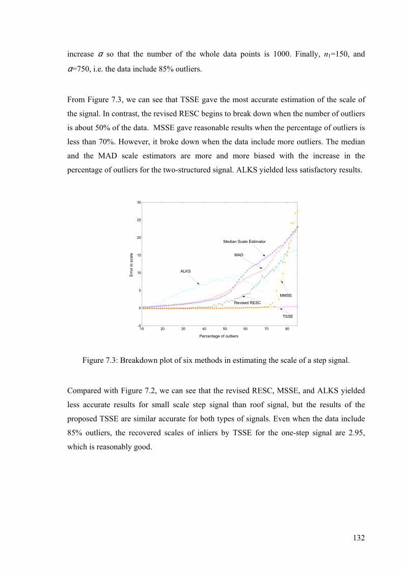
132
increase α so that the number of the whole data points is 1000. Finally, n1=150, and
α=750, i.e. the data include 85% outliers.
From Figure 7.3, we can see that TSSE gave the most accurate estimation of the scale of
the signal. In contrast, the revised RESC begins to break down when the number of outliers
is about 50% of the data. MSSE gave reasonable results when the percentage of outliers is
less than 70%. However, it broke down when the data include more outliers. The median
and the MAD scale estimators are more and more biased with the increase in the
percentage of outliers for the two-structured signal. ALKS yielded less satisfactory results.
10 20 30 40 50 60 70 80 -5
0
5
10
15
20
25
30
Percentage of outliers
Erro
r in
scal
e
TSSE
ALKS
Median Scale Estimator
MAD
Revised RESC
MMSE
Figure 7.3: Breakdown plot of six methods in estimating the scale of a step signal.
Compared with Figure 7.2, we can see that the revised RESC, MSSE, and ALKS yielded
less accurate results for small scale step signal than roof signal, but the results of the
proposed TSSE are similar accurate for both types of signals. Even when the data include
85% outliers, the recovered scales of inliers by TSSE for the one-step signal are 2.95,
which is reasonably good.

133
0 10 20 30 40 50 60 70 80 90 100 1100
5
10
15
20
25
30
35
40
S(0.5)
S(0.4)
S(0.3)
S(0.2)
S(0.1)
7.4.4.3 Breakdown Plot for Robust Scale Estimator
If the data have a Gaussian like distribution, the median scale estimator ( 7.1) is only one
possible robust k scale estimator ( 2.31) (corresponding to k=0.5n). We investigated the
achievements of the robust k scale estimator (assuming the correct parameters of a model
have been found). Let:
]2/)1[(
ˆ)( 1 q
dqS q
+Φ= − ( 7.12)
where q is set from 0 to 1. Thus S (0.5) is the median scale estimator.
We generated a one-step signal containing 500 data points in total. One-step signal: x:(0-
55), y=30, n1, σ=1; x:(55-100), y=40, n2=50; σ=1. At the beginning, n1 = 450 and α =0;
Then, we decrease n1, and at the same time, we increase α until n1=50, and α=400, i.e. the
data include 90% outliers.
Figure 7.4: Breakdown plot of different robust k scale estimators.
As Figure 7.4 shows, after finding the robust estimate of the parameters of a model, the
accuracy of S (q) is increased with the decrease of q. When the outliers are less than 50%
of the whole data, the difference for different values of q is small. However, when the data

134
include more than 50% outliers, the difference for various values of q is large. This
provides a useful cue for robust estimators, which use the median scale method to recovery
the scale of inliers.
7.4.4.4 Performance of TSSE
From the experiments in this section, we can see the proposed TSSE is a very robust scale
estimator, achieving better results than the other five methods. However, we must
acknowledge that the accuracy of TSSE is related to the accuracy of kernel density
estimation. In particular, for very few data points, the kernel density estimates will be less
accurate. Also, the proposed TSSE may underestimate the scale if the underlying
distribution is composed of heavily overlapping Gaussians
We also note that, for the purposes of this chapter (only), we assume we know the
parameters of the model: this is so we can concentrate on estimating the scale of the
residuals. However, in practice, one cannot directly estimate the scale: the parameters of a
model also need to be estimated. In the next chapter, we will propose a new robust
estimator—Adaptive Scale Sample Consensus (ASSC) estimator, which can estimate the
parameters and the scale simultaneously.
7.5 Conclusions
In this chapter, we show that scale estimation for data, involving multiple structures and
high percentages of outliers, is as yet a relatively unsolved problem. This provides an
important warning to the computer vision community: it is necessary to carefully choose a
proper scale estimator.
We also, based on the mean shift algorithm, propose a simple but efficient mean shift
valley technique, which can be used to find local valley. Furthermore, we propose a
promising robust scale estimator (TSSE), based on the mean shift and the mean shift valley
techniques. The experiments are compared with five other state-of-the-art robust scale

135
estimators, and show the advantages of TSSE over these methods, especially, when the
data involve a high percentage of outliers and the noise level of inliers is large. TSSE is a
very general method and can be used to give an initial scale estimate for robust estimators
such as M-estimators, etc. TSSE can also be used to provide an auxiliary estimate of scale
(after the parameters of a model to fit have been found) as a component of almost any
robust fitting method such as Hough Transform (Hough 1962), MDPE (chapter 4) and
QMDPE (chapter 5), etc.
136
8. Robust Adaptive-Scale Parametric Model Estimation for Computer Vision
8.1 Introduction
Robust model fitting essentially requires the application of two estimators. The first is an
estimator for the values of the models parameters. The second is an estimator for the scale
of the noise in the (inlier) data. In the previous chapter, we proposed a novel robust scale
estimation technique: the Two-Step Scale estimator (TSSE) and shown the performance of
TSSE despite heavily contaminated data, assuming that the correct parameters of a model
are available. However, in many practical cases, the parameters of a model and the scale of
inliers need to be estimated simultaneously. In this chapter, based on our previous work
(TSSE), we will propose a novel robust estimator: Adaptive Scale Sample Consensus
(ASSC) estimator. The ASSC estimator combines Random Sample Consensus (RANSAC)
and TSSE. ASSC also uses a modified objective function that depends upon both the
number of inliers and the corresponding scale.
Discontinuous signals (such as parallel lines/planes, step lines/planes, etc.) often appear in
computer vision tasks. A lot of work has been done to investigate the behaviour of robust
estimators for discontinuous signals, e.g., (Miller and Stewart 1996; Stewart 1997; Stewart
1.1.7. Chapter 8
Robust Adaptive-Scale Parametric Model Estimation for Computer Vision

137
1999; Chen and Meer 2002). Discontinuous signals are hard to deal with: e.g., most robust
estimators break down and yield a “bridge” between the two planes of one step signal.
ASSC is very robust to discontinuous signals and data with multiple structures, being able
to tolerate more than 80% outliers.
The main advantage of ASSC over RANSAC is that prior knowledge about the scale of
inliers is not needed. ASSC can simultaneously estimate the parameters of a model and the
scale of inliers belonging to that model. Experiments on synthetic data show that ASSC
has better robustness to heavily corrupted data than Least Median Squares (LMedS),
Residual Consensus (RESC), and Adaptive Least K’th order Squares (ALKS). We also
apply ASSC to two fundamental computer vision tasks: range image segmentation and
robust fundamental matrix estimation. Experiments show very promising results.
At the latter part of this chapter, we extend ASSC to produce ASRC (Adaptive-Scale
Residual Consensus) estimator. ASRC scores a model based on both the residuals of inliers
and the corresponding scale estimate determined by those inliers. The difference between
ASRC and ASSC is: in ASSC, all inliers are treated as the same, i.e., each inlier
contributes 1 to the object function of ASSC. However, in ASRC, the sizes of the residuals
of inliers are influential.
The main contributions of this chapter can be summarized as follows:
• By employing TSSE in a RANSAC like procedure, we propose a highly robust
estimator: Adaptive Scale Sample Consensus (ASSC) estimator.
• Experiments presented show that ASSC is highly robust to heavily corrupted data
with multiple structures and discontinuities (empirically, ASSC can tolerate more
than 80% outliers), and that it outperforms several competing methods.
• ASSC is successfully applied in two fundamental and important computer vision
tasks: range image segmentation and fundamental matrix estimation. The
experiments show promising results.

138
• We extend ASSC to produce ASRC which improves the objective function of
ASSC by weighting each inlier differently according to the size of the residual of
that inlier. Experiments showing the advantages of ASRC over ASSC.
This chapter is organized as follows: in section 8.2, the robust ASSC estimator is proposed.
In section 8.3, experimental comparisons, using both 2D and 3D examples, are presented.
We apply ASSC to range image segmentation in section 8.4 and fundamental matrix
estimation in section 8.5. We introduce ASRC and we provide some experiments showing
the advantages of ASRC over ASSC in section 8.6. We state our conclusions in section 8.7.
8.2 Adaptive Scale Sample Consensus (ASSC) Estimator
Algorithm
In section 2.4.3 we reviewed the RANSAC estimator. The criterion used by RANSAC is to
maximize the number of data points within the user-set error bound. Clearly, this bound is
related to the scale of the inliers (S). Mathematically, the RANSAC estimate can be written
as:
θθθ ˆˆ
maxargˆ n= ( 8.1)
where θn is the number of points whose absolute residual in the candidate parameter space
is within the error bound (i.e., Sr 5.2≤ ));θ is the estimated parameters from one of the
randomly chosen p-subsets.
The error bound in RANSAC is crucial to the performance of RANSAC. Provided with a
correct error bound of inliers, the RANSAC method can find a model even when data
contain a large percentage of gross errors. However, when the wrong error bound is given,
RANSAC will totally break down even when outliers occupy relatively small percentages
of the whole data (see section 4.4.4.2). Thus the major problem with RANSAC is that the

139
technique needs priori knowledge of the error bound of inliers, which is not available in
most practical vision tasks.
In this section, we will, based upon our previously proposed TSSE, propose an adaptive-
scale robust estimator — ASSC. We assume that when a model is correctly found, two
criteria should be satisfied:
• The number of data points (nθ) near or on the model should be as large as possible;
• The residuals of the inliers should be as small as possible. Correspondingly, the
scale (Sθ) should be as small as possible.
We therefore define our objective function as:
)/(maxargˆˆˆˆ θθθ
θ Sn= ( 8.2)
Note: when the estimate of the scale is fixed, equation ( 8.2) is another form of RANSAC
with the score nθ scaled by 1/S (i.e, a fixed constant for all p-subsets), yielding the same
results as RANSAC. ASSC is more reasonable than RANSAC because the scale is
estimated for each candidate fit, in addition to the fact that it no longer requires a user
defined error-bound.
The ASSC algorithm is as follows:
(1) Randomly choose one p-subset from the data points, estimate the model parameters
using the p-subset, and calculate the ordered absolute residuals of all data points.
(2) Choose the bandwidth by equation 6.6 and calculate an initial scale by a robust k
scale estimator (equation 7.12) using q=0.2.
(3) Apply TSSE to the absolute sorted residuals to estimate the scale of inliers. At the
same time, the probability density at the local peak )(ˆ peakf and local valley
)(ˆ valleyf are obtained by equation ( 4.1).

140
(4) Validate the valley. Let )(ˆ valleyf / )(ˆ peakf = λ (where 1>λ ≥0). Because the
inliers are assumed to have a Gaussian-like distribution, the valley is not
sufficiently deep when λ is too large (say, 0.8). If the valley is sufficiently deep, go
to step (5); otherwise go to step (1).
(5) Calculate the score, i.e., the objective function of the ASSC estimator.
(6) Repeat step (1) to step (5) many times. Finally, output the parameters and the scale
S1 with the highest score.
Because the robust k scale estimator is biased for data with multiple structures, the final
scale of inliers S2 should be refined when the scale S1 obtained by TSSE is used. In order to
improve the statistical efficiency, a weighted least square procedure ((Rousseeuw and
Leroy 1987), p.202) is carried out after finding the initial fit.
Instead of estimating the fit involving the absolute majority in the data set, the ASSC
estimator finds a fit having a relative majority of the data points. This makes it possible, in
practice, for ASSC to obtain a high robustness so that it can tolerate more than 50%
outliers. Indeed, the experiments in the next section show that the ASSC estimator is a very
robust estimator for data with multiple structures and a high percentage of outliers.
8.3 Experiments with Data Containing Multiple Structures
In this section, both 2D and 3D examples are given. The results of the proposed method are
compared with those of three other popular methods: LMedS, RESC, and ALKS. All of the
four methods use the random sampling scheme that is also at the heart of our method.
Note: unlike the experiments in section 7.4, here we do not (of course) assume any
knowledge of the parameters of the models in the data. Nor are we aiming to find any
particular structure. Due to the random sampling used, the methods will possibly return a
different structure on different runs – however, they will generally find the largest
structure most often (if one dominates in size).

141
10 20 30 40 50 60 70 80 90 100
10 20 30 40 50 60 70 80 90
100
LMedS ALKS
RESC
ASSC
10 20 30 40 50 60 70 80 90 100
10
20
30
40
50
60
70
80
90
100
LMedS
ALKS
RESC
ASSC
10 20 30 40 50 60 70 80 90 100
10 20 30 40 50 60 70 80 90
100
ASSC and RESC
LMedS
ALKS
10 20 30 40 50 60 70 80 90 100
10
20
30
40
50
60
70
80
90
100
LMedS
ALKS
RESC ASSC
8.3.1 2D Examples
(a) (b)
(c) (d)
Figure 8.1: Comparing the performance of four methods: (a) fitting a line with a total of
90% outliers; (b) fitting three lines with a total of 88% outliers; (c) fitting a step with a
total of 85% outliers; (d) fitting three steps with a total of 89% outliers.
We generated four kinds of data (a line, three lines, a step, and three steps), each with a
total of 500 data points. The signals were corrupted by Gaussian noise with zero mean and
standard variance σ. Among the 500 data points, α data points were randomly distributed
in the range of (0, 100). The i'th structure has ni data points.
(a) One line: x:( 0-100), y=x, n1=50; α=450; σ=0.8.
(b) Three lines: x:(25-75), y=75, n1=60; x:(25-75), y=60, n2=50; x=25, y:(20-75),
n3=40; α=350; σ=1.0.

142
(c) One step: x:(0-50), y=35, n1=75; x:(50-100), y=25, n2=55; α=370; σ=1.1.
(d) Three steps: x:(0-25), y=20, n1=55; x:(25-50), y=40, n2=30; x:(50-75), y=60, n3=30;
x:(75-100), y=80, n4=30; α=355; σ=1.0.
In Figure 8.1, we can see that the proposed ASSC method yields the best results among the
four methods, correctly fitting all four signals. Because LMedS has a 50% breakdown
point, it failed to fit all the four signals. Although ALKS can tolerate more than 50%
outliers, it failed in all four cases with very high outlier content. RESC gave better results
than LMedS and ALKS. It succeeded in two cases (one-line and three-line signals) even
when the data involved more than 88% outliers. However, RESC failed to fit two signals
(Figure 8.1 (c) and (d)).
It should be emphasized that both the bandwidth choice and the scale estimation in the
proposed ASSC method are data-driven. No prior knowledge about the bandwidth and the
scale is necessary in the proposed method. This is a great improvement over the traditional
RANSAC method where the user must set a priori scale-related error bound.
8.3.2 3D Examples
Two synthetic 3D signals were generated. Each contained 500 data points and three planar
structures. Each plane contains 100 points corrupted by Gaussian noise with standard
variance σ; 200 points are randomly distributed in a region including all three structures. A
planar equation can be written as Z=AX+BY+C, and the residual of the point at (Xi, Yi, Zi) is
ri=Zi-AXi-BYi-C. (A, B, C; σ) are the parameters to estimate.
In contrast to the section 8.3.1, we now attempt to find all structures in the data. In order to
extract all planes, we:
(1) Apply the robust estimators to the data set and estimate the parameters and scale of a
plane;
(2) Extract the inliers and remove them from the data set;
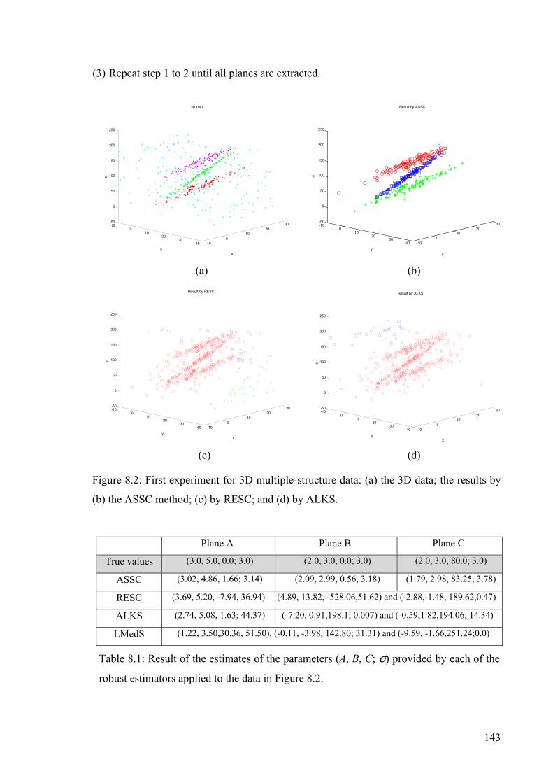
143
-100
1020
30-100
1020
3040
-50
0
50
100
150
200
250
x
Result by RESC
y
z
-100
1020
30-100
1020
3040
-50
0
50
100
150
200
250
x
Result by ALKS
y
z
-100
1020
30-100
1020
3040
-50
0
50
100
150
200
250
x
3D Data
y
z
-10 0 1020
30-100
1020
30 40
-50
0
50
100
150
200
250
x
Result by ASSC
y
z
(3) Repeat step 1 to 2 until all planes are extracted.
(a) (b)
(c) (d)
Figure 8.2: First experiment for 3D multiple-structure data: (a) the 3D data; the results by
(b) the ASSC method; (c) by RESC; and (d) by ALKS.
Plane A Plane B Plane C
True values (3.0, 5.0, 0.0; 3.0) (2.0, 3.0, 0.0; 3.0) (2.0, 3.0, 80.0; 3.0)
ASSC (3.02, 4.86, 1.66; 3.14) (2.09, 2.99, 0.56, 3.18) (1.79, 2.98, 83.25, 3.78)
RESC (3.69, 5.20, -7.94, 36.94) (4.89, 13.82, -528.06,51.62) and (-2.88,-1.48, 189.62,0.47)
ALKS (2.74, 5.08, 1.63; 44.37) (-7.20, 0.91,198.1; 0.007) and (-0.59,1.82,194.06; 14.34)
LMedS (1.22, 3.50,30.36, 51.50), (-0.11, -3.98, 142.80; 31.31) and (-9.59, -1.66,251.24;0.0)
Table 8.1: Result of the estimates of the parameters (A, B, C; σ) provided by each of the
robust estimators applied to the data in Figure 8.2.

144
-100
1020
30
-10 0 10 20 30 40 50
-20
0
20
40
60
80
100
120
xy
z
3D Data
-100
1020
30
-10 0 10 20 30 40 50
-20
0
20
40
60
80
100
120
x
Result by RESC
y
z
-100
1020
30
-10 0 10 20 30 40 50
-20
0
20
40
60
80
100
120
x
Result by ALKS
y
z
-10 0 1020
30
-10 0 10 20 30 40 50 -20
0
20
40
60
80
100
120
x
Result by ASSC
y
z
(a) (b)
(c) (d)
Figure 8.3: Second experiment for 3D multiple-structure data: (a) the 3D data; the results
by (b) the proposed method; (c) by RESC; (d) and by ALKS.
Plane A Plane B Plane C
True values (0.0, 3.0, -60.0; 3.0) (0.0, 3.0, 0.0; 3.0) (0.0, 0.0, 40.0; 3.0)
ASSC (0.00, 2.98, -60.68, 2.11) (0.18, 2.93, 0.18, 3.90) (0.08, 0.03, 38.26; 3.88)
RESC (0.51, 3.04,-67.29;36.40) (6.02,-34.00,-197.51;101.1) and (0.35, -3.85, 122.91, 0.02)
ALKS (-1.29, 1.03,14.35; 30.05), (-1.07, -2.07,84.31; 0.01) and (1.85, -11.19, 36.97; 0.08)
LMedS (0.25, 0.61,24.50, 27.06), (-0.04, -0.19, 92.27; 9.52) and (-0.12, -0.60,92.19; 6.89)
Table 8.2: Result of the estimates of the parameters (A, B, C; σ) provided by each of
the robust estimators applied to the data in Figure 8.3.

145
The red circles constitute the first plane extracted; the green stars the second plane
extracted; and the blue squares the third extracted plane. The results are shown in Figure
8.2, Table 8.1; Figure 8.3 and Table 8.2 (the results of LMedS, which completely broke
down for these 3D data sets, are only given in Table 8.1 and Table 8.2). Note for RESC,
we use the revised form in equation ( 7.6) instead of equation ( 7.5) for scale estimate.
Similarly, in the second experiment (Figure 8.3 and Table 8.2), LMedS and ALKS
completely broke down for the heavily corrupted data with multiple structures. RESC,
although it correctly fitted the first plane, wrongly estimated the scale of the inliers to the
plane. RESC wrongly fitted the second and the third planes. Only the proposed method
correctly fitted all three planes (Figure 8.3 (b)) and estimated the corresponding scale for
each plane.
The proposed method is computationally efficient. We perform the proposed method in
MATLAB code with TSSE in Mex. When m is set as 500, the proposed method takes
about 1.5 second for the 2D examples and about 2.5 seconds for the 3D examples in an
AMD 800MHz personal computer.
8.3.3 The Breakdown Plot of the Four Methods
In this subsection, we perform an experiment to draw the breakdown plot of each method
(similar to the experiment reported in (Yu, Bui et al. 1994). However, the data that we use
is more complicated because it contains two types of outliers: clustered outliers and
randomly distributed outliers).
We generate one plane signal with Gaussian noise having unit standard variance. Both
clustered outliers and randomly distributed outliers are added to the data. The clustered
outliers have 100 data points and are distributed within a cube. The randomly distributed
outliers contain the plane signal and clustered outliers. The number of inliers is decreased
from 900 to 100. At the same time, the number of randomly distributed outliers is
increased from 0 to 750 so that the total number of the data points is kept 1000. Thus, the
outliers occupy from 10% to 90% outliers. Examples for data with 20% and 70% outliers
are shown in Figure 8.4 (a) and (b) to illustrate the distributions of the inliers and outliers.

146
-5
0
5
10
15
-10 0 10 20 30 40 50
-10
0
10
20
30
40
50
60
70
Data distribution involving 20% outliers
x
z
y
Clustered Outliers
Inliers
Random outliers
0 10 20 30 40 50 60 70 80 90-0.2
0
0.2
0.4
0.6
0.8
1
1.2
1.4
Outlier Percentage
Err
or in
B
ASSCRESCALKSLMedS
LMedS
ALKS
RESC
ASSC
0 10 20 30 40 50 60 70 80 90-15
-10
-5
0
5
10
15
Outlier Percentage
Erro
r in
C
ASSC RESC ALKS LMedS
LMedS
ALKS
RESC
ASSC
0 10 20 30 40 50 60 70 80 90 -1.5
-1
-0.5
0
0.5
1
1.5
Outlier Percentage
Erro
r in
A
ASSC RESC ALKS LMedS
If an estimator is robust enough to outliers, it can resist the influence of both clustered
outliers and randomly distributed outliers even when the outliers occupy more than 50% of
the data. In order to increase the stability of the result, we perform the experiments 20
times, using different random sampling seeds, for each data set involving different
percentage of outliers (10% to 90%). An averaged result is show in Figure 8.4 (c-e).
(a) (b)
(c) (d) (e)
Figure 8.4: Breakdown plot of the four methods: (a) example of the data with 20% outliers;
(b) example of the data with 80% outliers; (c) the error in the estimate of parameter A, (d)
in parameter B, and (e) in parameter C.
From Figure 8.4 (c-e), we can see that our method obtains the best result. Because the
LMedS has only 50% breakdown point, it broke down when outliers occupied more than
50% of the data (approximately). ALKS broke down when outliers had about 75%. RESC
began to break down when outliers had more than 83% of the whole data; In contrast, the
ASSC estimator is the most robust to outliers. It began to breakdown at 89% outliers. In
fact, when the inliers are about (or less than) 10% of the data, the assumption that inliers
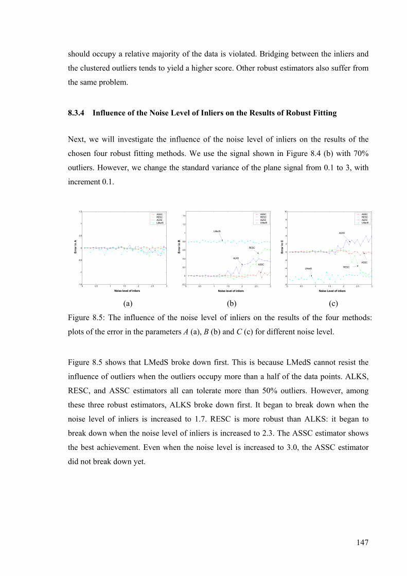
147
should occupy a relative majority of the data is violated. Bridging between the inliers and
the clustered outliers tends to yield a higher score. Other robust estimators also suffer from
the same problem.
8.3.4 Influence of the Noise Level of Inliers on the Results of Robust Fitting
Next, we will investigate the influence of the noise level of inliers on the results of the
chosen four robust fitting methods. We use the signal shown in Figure 8.4 (b) with 70%
outliers. However, we change the standard variance of the plane signal from 0.1 to 3, with
increment 0.1.
(a) (b) (c)
Figure 8.5: The influence of the noise level of inliers on the results of the four methods:
plots of the error in the parameters A (a), B (b) and C (c) for different noise level.
Figure 8.5 shows that LMedS broke down first. This is because LMedS cannot resist the
influence of outliers when the outliers occupy more than a half of the data points. ALKS,
RESC, and ASSC estimators all can tolerate more than 50% outliers. However, among
these three robust estimators, ALKS broke down first. It began to break down when the
noise level of inliers is increased to 1.7. RESC is more robust than ALKS: it began to
break down when the noise level of inliers is increased to 2.3. The ASSC estimator shows
the best achievement. Even when the noise level is increased to 3.0, the ASSC estimator
did not break down yet.
0 0.5 1 1.5 2 2.5 3-0.2
0
0.2
0.4
0.6
0.8
1
1.2
1.4
Noise level of inliers
Erro
r in
B
ASSCRESCALKSLMedS
LMedS
ALKS
RESC
ASSC
0 0.5 1 1.5 2 2.5 3-8
-6
-4
-2
0
2
4
6
8
10
Noise Level of inliers
Erro
r in
C
ASSCRESCALKSLMedS
LMedS
ALKS
RESC
ASSC
0 0.5 1 1.5 2 2.5 3 -1.5
-1
-0.5
0
0.5
1
1.5
Noise level of inliers
Erro
r in
A
ASSC RESC ALKS LMedS

148
-5 0 5 10 15-20
0
20-10
0
10
20
30
40
50
x
Parallel planes
y
z
-5
0
5
10
15-10 -5 0 5 10 15 20 25 30
-10
0
10
20
30
40
50 Step Signal
yx
z
0 2 4 6 8 10 12 14 16 18 20 -1
-0.8
-0.6
-0.4
-0.2
0
0.2
0.4
0.6
0.8
1
Step height
Erro
r in
A
ASSC RESC ALKS LMedS
0 2 4 6 8 10 12 14 16 18 20-0.2
0
0.2
0.4
0.6
0.8
1
1.2
1.4
1.6
1.8
Step height
Erro
r in
B
ASSCRESCALKSLMedS
LMedS
RESC
ALKS
ASSC
0 2 4 6 8 10 12 14 16 18 20-6
-5
-4
-3
-2
-1
0
1
2
3
Step height
Erro
r in
C
ASSCRESCALKSLMedS
LMedS
ALKS
RESC
ASSC
8.3.5 Influence of the Relative Height of Discontinuous Signals
In this subsection, we will investigate the influence of the relative height of discontinuous
signals on the performance of the four methods.
(a) (b)
(c1) (c2) (c3)
(d1) (d2) (d3)
Figure 8.6: The influence of the relative height of discontinuous signals on the results of
the four methods: (a) two parallel planes; (b) one step signal; (c1-c3) the results for the two
parallel planes; (d1-d3) the results for the step signal.
0 2 4 6 8 10 12 14 16 18 20 -1
-0.8
-0.6
-0.4
-0.2
0
0.2
0.4
0.6
0.8
1
Parallel height
Erro
r in
A
ASSC RESC ALKS LMedS
0 2 4 6 8 10 12 14 16 18 20
-0.4
-0.2
0
0.2
0.4
0.6
Parallel height
Erro
r in
B
ASSCRESCALKSLMedS
LMedS
ALKS
RESC
ASSC
0 2 4 6 8 10 12 14 16 18 20-2
0
2
4
6
8
10
12
Parallel height
Erro
r in
C
ASSC RESC ALKS LMedS
LMedS ALKS
RESC
ASSC

149
We generate two discontinuous signals: one containing two parallel planes and one
containing one-step planes. The signals have unit variance. Randomly distributed outliers
covering the regions of the signals are added to the signals. Among the total 1000 data
points, there are 20% pseudo-outliers and 50% random outliers. The relative height is
increased from 1 to 20. Figure 8.6 (a) and (b) shows examples of the data distributions of
the two signals with relative height 10. The averaged results (over 20 repetitions) obtained
by the four robust estimators are shown in Figure 8.6 (c1-c3) and (d1-d3).
From Figure 8.6, we can see the tendency to bridge becomes stronger as the step decreases.
LMedS shows the worst results among the four robust estimators. For the rest three
estimators: ASSC, ALKS, and RESC, from Figure 8.6 (c1-c3) and (d1-d3), we can see
that:
• For the parallel plane signal, the results by ALKS are affected most by the small
step. RESC shows better result than ALKS. However, ASSC shows the best result.
• For the step signal, when the step height is small, all of these three estimators are
affected. When the step height is increased from small to large, all of the three
estimators show robustness to the signal. However, ASSC achieves the best results for
small step height signals.
In next sections, we will apply the ASSC estimator to more "real world" computer vision
tasks: range image segmentation and fundamental matrix estimation.
8.4 ASSC for Range Image Segmentation
The range image segmentation algorithm that we present here is based on the just
introduced ASSC estimator. Although MDPE in chapter 4, has similar performance to
ASSC, MDPE only outputs the parameters of the model as results. An auxiliary scale
estimator is required to provide an estimate of the scale of inliers. ASSC, however, does
not need any auxiliary scale estimator at the post-processing stage. It can estimate the scale
of inliers during the process of estimating the parameters of a model.

150
8.4.1 The Algorithm of ASSC-Based Range Image Segmentation
We employ a hierarchical structure, similar to that in chapter 5. We begin with bottom
level containing 64x64 pixels that are obtained by using regular sampling on the original
512x512 image. In each level of the hierarchy, we:
(1) Apply the ASSC estimator to obtain the parameters of plane and the scale of inliers.
(2) The inliers (in the top hierarchy) corresponding to the estimated parameters of plane
and scale are then identified. If the number of inliers is less than a threshold, go to step
(7). This step is different from the step (4) in section 5.4.2 in that the parameters of
plane and the corresponding scale of inliers are obtained simultaneously in ASSC;
while QMDPE needs an auxiliary scale estimator to obtain the scale of inliers.
(3) Use normal information to validate the inliers obtained in step (2). This step is similar
to the step (5) in section 5.4.2. If the number of the validated inliers is small, go to step
(7).
(4) Fill in the holes inside the maximum connected component from the validated inliers.
The holes may appear because of sensor noise or because some points have large
residuals and are beyond the range that is related to the estimated scale.
(5) Assign a label to the points corresponding to the connected component from step (4)
and remove the points from the data set that will be further processed. This happens in
the top of the hierarchy.
(6) If a point is unlabelled and it is not a jump edge point, the point will be used as a "left-
over" point. After collecting all these points, use the connected component algorithm to
get the maximum connected component. If the number data points of the maximum
connected component of "left-over" points is smaller than a threshold, go to step (7);
otherwise, get the data for the current hierarchical level by regularly sampling on the
maximum connected component obtained in this step, then go to step (1).
(7) Terminate the processing in the current level of the hierarchy and go to the higher-level
hierarchy until the top of the hierarchy.
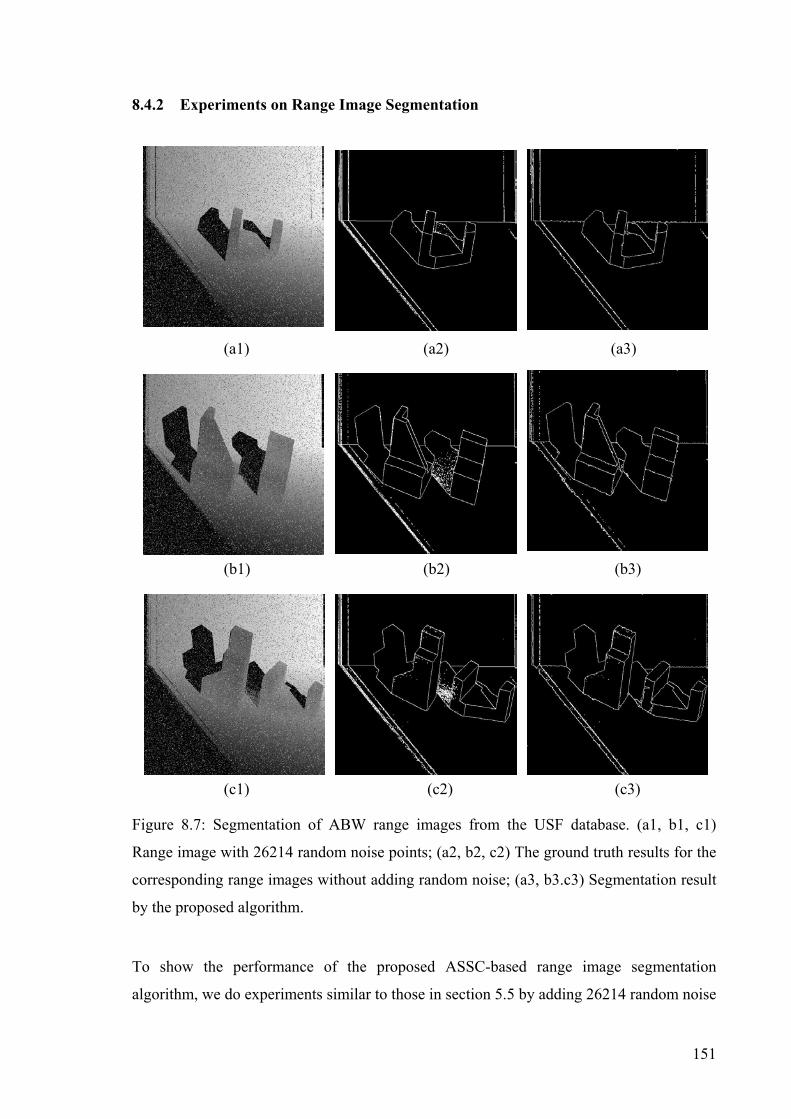
151
8.4.2 Experiments on Range Image Segmentation
(a1) (a2) (a3)
(b1) (b2) (b3)
(c1) (c2) (c3)
Figure 8.7: Segmentation of ABW range images from the USF database. (a1, b1, c1)
Range image with 26214 random noise points; (a2, b2, c2) The ground truth results for the
corresponding range images without adding random noise; (a3, b3.c3) Segmentation result
by the proposed algorithm.
To show the performance of the proposed ASSC-based range image segmentation
algorithm, we do experiments similar to those in section 5.5 by adding 26214 random noise

152
points to the range images taken from the USF ABW range image database (test 16, test 7
and train 5).
As shown in Figure 8.7, all of the main surfaces (structures) were recovered by our
method. Only a slight distortion appeared on some boundaries of neighbouring surfaces.
Similar slight distortion also appears in the experimental results (by QMDPE) in chapter 5.
This is because of the sensor noise and the limited accuracy of the estimated normal at
each range point. Generally speaking, the more accurate the range data are, and the more
accurate the estimated normal at range points is, the less the distortion is.
(a) (b) (c)
(d) (e) (f)
Figure 8.8: Comparison of the segmentation results for ABW range image (test 3) from the
USF range image database. (a) Range image; (b) The result of ground truth; (c) The result
by the USF;(d) The result by the WSU; (e) The result by the UE; (f) The result by the
proposed method.

153
We also compare our results with those of the University of South Florida (USF),
Washington State University (WSU), and the University of Edinburgh (UE) (Hoover, Jean-
Baptiste et al. 1996) methods. Figure 8.8(c-f) and Figure 8.9 (c-f) show the results obtained
by the four methods. From Figure 8.8 (c) and Figure 8.9 (c), we can see that the USF’s
results contained many noisy points. In both Figure 8.8 (d) and Figure 8.9 (d), the WSU
segmenter missed one surface. The WSU segmenter also over segmented one surface in
Figure 8.8 (d). Some boundaries on the junction of the segmented patch by the USF and
WSU in Figure 8.9 (c) were relatively seriously distorted. The UE shows relatively better
results than the USF and the WSU. However, some estimated surfaces are still noisy (see
Figure 8.8 (e) and Figure 8.9 (e)). Compared with the other three methods, the proposed
method achieved the best results. All surfaces are recovered and the segmented surfaces
are relatively “clean”. The edges of the segmented patches were reasonably good.
(a) (b) (c)
(d) (e) (f)
Figure 8.9: Comparison of the segmentation results for ABW range image (test 13) from
the USF range image database. (a) Range image; (b) The result of ground truth; (c) The
result by the USF; (d) The result by the WSU; (e) The result by the UE; (f) The result by
the proposed method.
154
8.5 ASSC for Fundamental Matrix Estimation
8.5.1 Background of Fundamental Matrix Estimation
The fundamental matrix provides some constraints (related to epipolar geometry,
projectivity, etc.) between corresponding points in multiple views. The estimation of the
fundamental matrix is important for several problems: matching, recovering of structure,
motion segmentation, etc.(Torr and Zisserman 2000). Since there possibly are mismatched
pairs of points in the data, traditional method such as least squares estimator cannot yield
accurate results. Even worse, the least squares estimator can breakdown. Robust estimators
such as M-estimators, LMedS, RANSAC, MSAC and MLESAC have been applied to
estimate the fundamental matrix to improve the accuracy of the results (Torr and Murray
1997).
Let {xi,} and {xi’} (for i=1,…,n) be a set of matched homogeneous image points viewed in
image 1 and image 2 respectively. We have the following constraints for the fundamental
matrix F:
' 0 det[ ] 0Ti ix Fx and F= = ( 8.3)
We employ the 7-point algorithm (Torr and Murray 1999) to solve for candidate fits
using Sampson distance for the residual to a fitted fundamental matrix. For the i’th
correspondence, the residual ri using Simpson distance is:
( )1/ 22 2 2 2' '
ii
x y x y
krk k k k
=+ + +
( 8.4)
8.5.2 The Experiments on Fundamental Matrix Estimation
First, we generated 300 matches including 120 point pairs of inliers with unit Gaussian
variance and 160 point pairs of random outliers. In practice, the scale of inliers is not
' ' ' ' ' ' 21 2 3 4 5 6 7 8 9i i i i i i i i i i i i iwhere k f x x f x y f x f y x f y y f y f x f y fς ς ς ς ς= + + + + + + + +
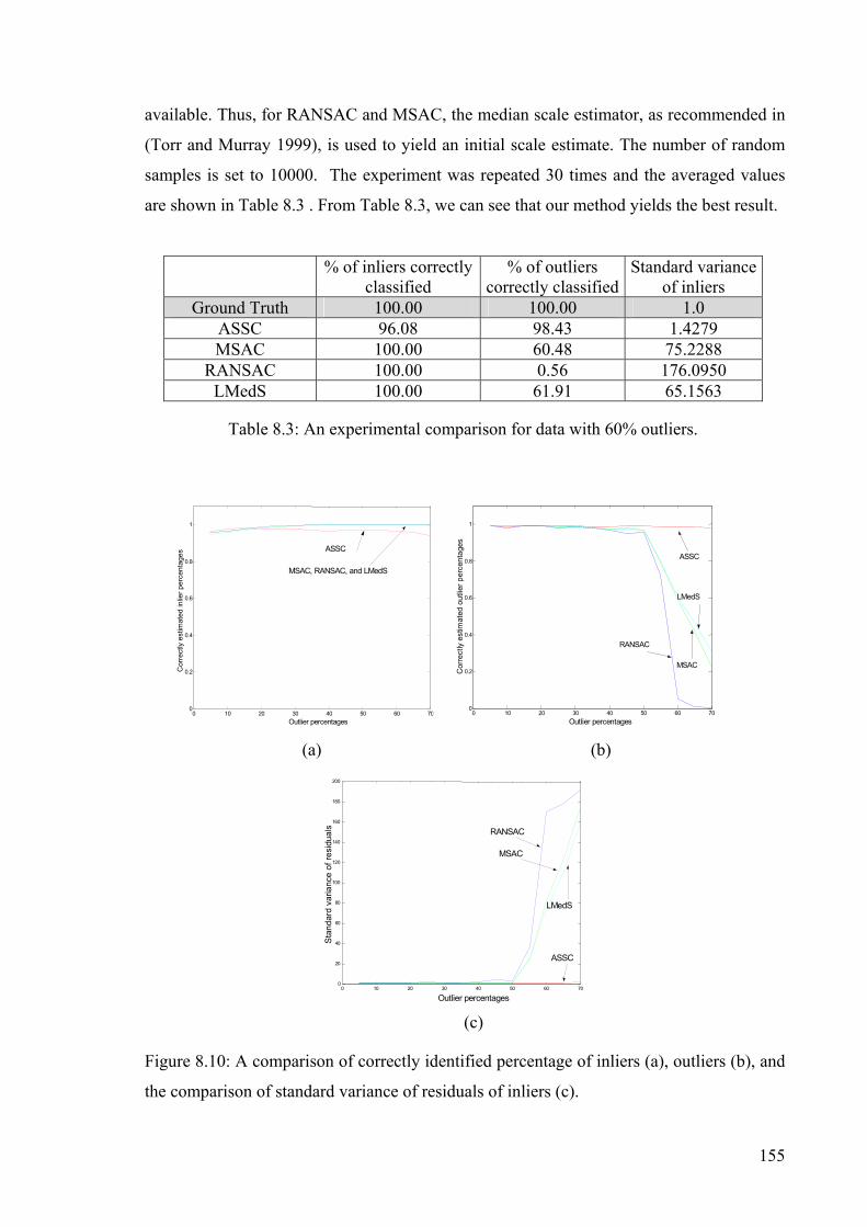
155
0 10 20 30 40 50 60 700
0.2
0.4
0.6
0.8
1
Outlier percentages
Cor
rect
ly e
stim
ated
inlie
r per
cent
ages
ASSC
MSAC, RANSAC, and LMedS
0 10 20 30 40 50 60 70 0
0.2
0.4
0.6
0.8
1
Outlier percentages
Cor
rect
ly e
stim
ated
out
lier p
erce
ntag
es
ASSC
RANSAC MSAC
LMedS
0 10 20 30 40 50 60 700
20 40 60 80
100 120 140 160 180 200
Outlier percentages
Sta
ndar
d va
rianc
e of
resi
dual
s
ASSC
RANSAC
MSAC
LMedS
available. Thus, for RANSAC and MSAC, the median scale estimator, as recommended in
(Torr and Murray 1999), is used to yield an initial scale estimate. The number of random
samples is set to 10000. The experiment was repeated 30 times and the averaged values
are shown in Table 8.3 . From Table 8.3, we can see that our method yields the best result.
(a) (b)
(c)
Figure 8.10: A comparison of correctly identified percentage of inliers (a), outliers (b), and
the comparison of standard variance of residuals of inliers (c).
% of inliers correctly classified
% of outliers correctly classified
Standard variance of inliers
Ground Truth 100.00 100.00 1.0 ASSC 96.08 98.43 1.4279 MSAC 100.00 60.48 75.2288
RANSAC 100.00 0.56 176.0950 LMedS 100.00 61.91 65.1563
Table 8.3: An experimental comparison for data with 60% outliers.
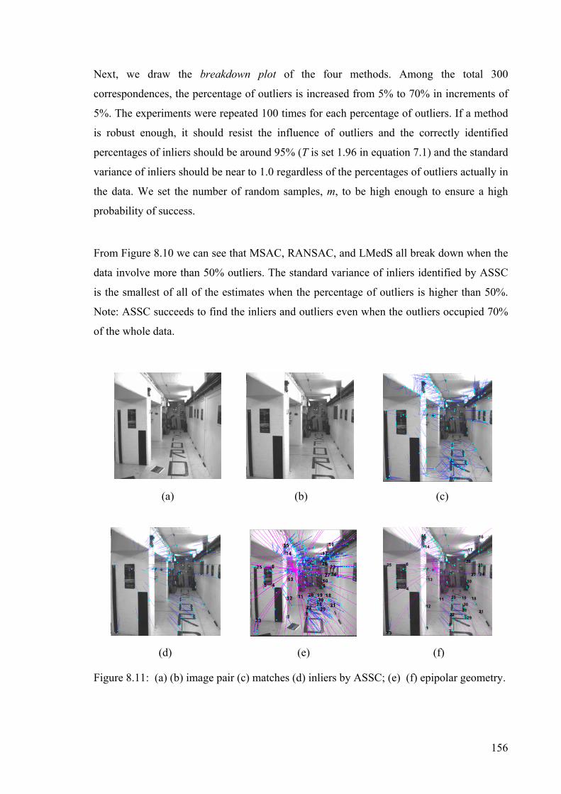
156
12 3
45
6
78
910
1112
13
14
15 16
17
181920
2122
23
24
2526
27
28
29
30
Next, we draw the breakdown plot of the four methods. Among the total 300
correspondences, the percentage of outliers is increased from 5% to 70% in increments of
5%. The experiments were repeated 100 times for each percentage of outliers. If a method
is robust enough, it should resist the influence of outliers and the correctly identified
percentages of inliers should be around 95% (T is set 1.96 in equation 7.1) and the standard
variance of inliers should be near to 1.0 regardless of the percentages of outliers actually in
the data. We set the number of random samples, m, to be high enough to ensure a high
probability of success.
From Figure 8.10 we can see that MSAC, RANSAC, and LMedS all break down when the
data involve more than 50% outliers. The standard variance of inliers identified by ASSC
is the smallest of all of the estimates when the percentage of outliers is higher than 50%.
Note: ASSC succeeds to find the inliers and outliers even when the outliers occupied 70%
of the whole data.
(a) (b) (c)
(d) (e) (f)
Figure 8.11: (a) (b) image pair (c) matches (d) inliers by ASSC; (e) (f) epipolar geometry.

157
To conclude, we apply the proposed method on real image frames. Two frames of the
Corridor sequence (bt.003 and bt.006), which can be obtained from
http://www.robots.ox.ac.uk/~vgg/data/ (Figure 8.11 (a) and (b)). Figure 8.11 (c) shows the
matches involving 500 point pairs in total. The inliers (201 correspondences) obtained by
the proposed method are shown in Figure 8.11 (d). The epipolar lines (we draw 30 of the
epipolar lines) and epipole using the estimated fundamental matrix by ASSC are shown in
Figure 8.11 (e) and (f). We can see that the proposed method achieves a good result.
Because the camera matrices of the two frames are available, we can obtain the ground
truth fundamental matrix and thus evaluate the errors. From Table 8.4, we can see that
ASSC performs the best among the four methods.
8.6 A Modified ASSC (ASRC)
8.6.1 Adaptive-Scale Residual Consensus (ASRC)
In the previous experiments, we have seen the robustness of ASSC to outliers and multiple
structures. However, all inliers in ASSC (equation 8.2), are treated as the same, i.e., each
inlier contributes equivalently to the objective function of ASSC. Actually, inliers can have
different influence on the results if we take into account the sizes of the residuals of inliers.
Thus, we modify ASSC to yield a robust adaptive-scale residual consensus (ASRC)
estimator.
Number of inliers (i.e., matched correspondences)
Mean error of inliers
Standard variance of inliers
ASSC 201 0.0274 0.6103
MSAC 391 -1.3841 10.0091
RANSAC 392 -1.0887 10.1394
LMedS 372 -1.4921 9.5463
Table 8.4: Experimental results on two frames of the Corridor sequence.

158
10 20 30 40 50 60 70 80 90 100
10
20
30
40
50
60
70
80
90
100
ALKS
LMedS
RESC, ASSC, and ASRC
10 20 30 40 50 60 70 80 90 100
10
20
30
40
50
60
70
80
90
100
ASRC
ASSC RESC
LMedS
ALKS
10 20 30 40 50 60 70 80 90 100
10
20
30
40
50
60
70
80
90
100
ASRC
RESC and ASSC
LMedS
ALKS
10 20 30 40 50 60 70 80 90 100
10
20
30
40
50
60
70
80
90
100
ASRC
LMedS
RESC
ALKS
ASSC
))/(1(
(maxargˆˆ
1ˆˆ
ˆ
ˆ
θ
θθ
θ
θ
θS
TSrn
ii∑
=
−= ( 8.5)
where θn is the number of inliers which satisfies equation 7.1) for the fitted θ .
From equation ( 8.5), we can see that when the residual of a data point is zero, the point
contributes 1 to the objective function of ASRC; when the residual of a data point is equal
or larger than TSθ , it does not contribute anything to the objective function of ASRC.
8.6.2 Experiments
(a) (b)
(c) (d)
Figure 8.12: Comparing the performance of five methods: (a) fitting a roof with a total of
87% outliers; (b) fitting F-figure with a total of 92% outliers; (c) fitting a step with a total
of 91% outliers; (d) fitting three-step with a total of 91% outliers.
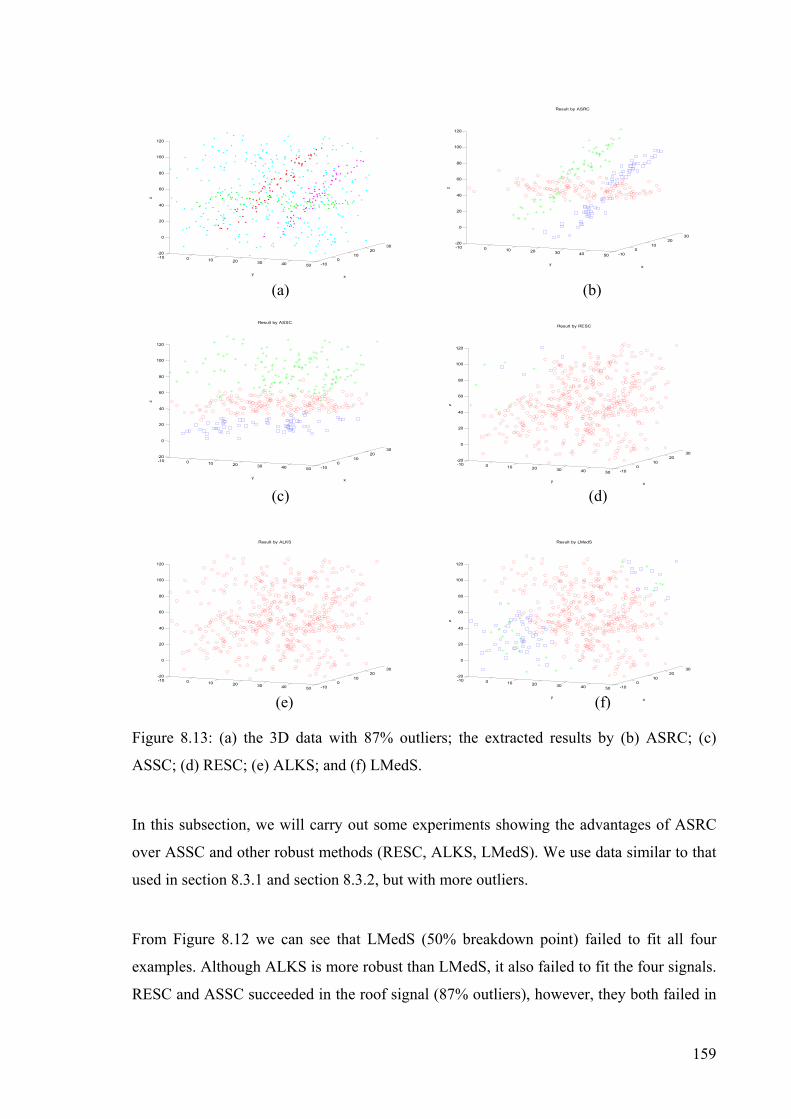
159
-100
1020
30
-10 0 10 20 30 40 50
-20
0
20
40
60
80
100
120
x
Result by RESC
y
z
-100
1020
30
-10 0 10 20 30 40 50
-20
0
20
40
60
80
100
120
Result by ALKS
-100
1020
30
-10 0 10 20 30 40 50
-20
0
20
40
60
80
100
120
x
Result by LMedS
y
z
-100
1020
30
-10 0 10 20 30 40 50
-20
0
20
40
60
80
100
120
x
Result by ASRC
y
z
-100
1020
30
-10 0 10 20 30 40 50
-20
0
20
40
60
80
100
120
xy
z
-100
1020
30
-10 0 10 20 30 40 50
-20
0
20
40
60
80
100
120
x
Result by ASSC
y
z
(a) (b)
(c) (d)
(e) (f)
Figure 8.13: (a) the 3D data with 87% outliers; the extracted results by (b) ASRC; (c)
ASSC; (d) RESC; (e) ALKS; and (f) LMedS.
In this subsection, we will carry out some experiments showing the advantages of ASRC
over ASSC and other robust methods (RESC, ALKS, LMedS). We use data similar to that
used in section 8.3.1 and section 8.3.2, but with more outliers.
From Figure 8.12 we can see that LMedS (50% breakdown point) failed to fit all four
examples. Although ALKS is more robust than LMedS, it also failed to fit the four signals.
RESC and ASSC succeeded in the roof signal (87% outliers), however, they both failed in

160
the other three cases. In contrast, ASRC correctly fits all four signals. ASRC doesn’t
breakdown even when outliers occupy more than 90%, which is an improvement over
ASSC.
From Figure 8.13 (d) and (e), we can see that RESC and ALKS, which claim to be robust
to data with more than 50% outliers, failed to extract the three planes. This is because the
estimated scales (by RESC and ALKS) for the first plane were wrong, which caused these
two methods to fail to fit the second and third planes. Because the LMedS (in Figure 8.13
(f)) has only a 50% breakdown point, it completely failed to fit data with such high
contamination — 80% outliers. ASSC, although it correctly fitted the first plane, wrongly
fitted the second and the third planes. Only the ASRC method correctly fitted and extracted
all three planes (Figure 8.13 (b)).
We also successfully applied the ASRC to range image segmentation and fundamental
matrix estimation, which is similar to those in section 8.4 and 8.5. We recommend reading
(Wang and Suter 2004) for details of those experiments.
8.7 Conclusion
In this chapter, we propose a very robust Adaptive Scale Sample Consensus (ASSC)
estimator. The ASSC method has an objective function that considers both the number of
inliers and the corresponding scale estimate for those inliers. ASSC is very robust to
multiple-structural data containing high percentages of outliers (more than 80% outliers).
The ASSC estimator is compared to several popular robust estimators: LMedS, RESC, and
ALKS and ASSC can generally achieve better results.
Furthermore, we applied ASSC to two important computer vision tasks: range image
segmentation and robust fundamental matrix estimation. However, the applications of
ASSC are not limited to these two fields. The computational cost of the proposed ASSC
method is moderately low, which makes it applicable to many computer vision tasks.

161
We also improved ASSC: ASRC improves the objective function of ASSC by weighting
each inlier differently according to the residual of that inlier.
Although we have compared against several of the “natural competitors” from the
computer vision and statistics literature (Fischler and Rolles 1981; Rousseeuw 1984; Yu,
Bui et al. 1994; Lee, Meer et al. 1998), it is difficult to be comprehensive. For example, in
(Scott 2001) the authors also proposed a method which can simultaneously estimate the
model parameters and the scale of the inliers. In essence, the method tries to find the fit
that produces residuals that are the most Gaussian distributed (or which have a subset that
is most Gaussian distributed), and all data points are considered; In contrast, only the data
points, within the band obtained by the mean shift and mean shift valley, are considered in
our objective function. Also, we do not assume the residuals for the best fit will be the best
match to a Gaussian distribution.
In the latter stage of proposing ASSC/ASRC, we become aware that Gotardo, et al.
proposed an improved robust estimator based on RANSAC and MLESAC (Gotardo,
Bellon et al. 2003), and applied it to range image segmentation. However, like RANSAC,
this estimator also requires that the user to set the scale-related tolerance a priori. In
contrast, the proposed ASSC/ASRC method in this chapter does not require any priori
information about the scale or tolerance. The parameters of a model and the corresponding
scale of inliers are simultaneously obtained from the data.

162
9. Mean shift for Image Segmentation by Pixel Intensity or Pixel
Color
9.1 Introduction
One major task of pattern recognition, image processing, and related areas: is to segment
image into homogenous regions. Image segmentation is the first step towards image
understanding and its success directly affects the quality of image analysis. Image
segmentation has been acknowledged to be one of the most difficult tasks in computer
vision and image processing (Cheng, Jiang et al. 2001; Comaniciu and Meer 2002a). Note:
the type of image we refer to in this chapter (grey/color) is different from that of the range
image we referred to in chapter 5 and chapter 8. A range image contains 3D geometry
information. That is, the value of a pixel in the range image corresponds to a depth/range
measurement.
Unlike other vision tasks such as parametric model estimation ((Wang and Suter 2003a;
Wang and Suter 2003b), also see chapter 3- 5 and chapter 8) , fundamental matrix
estimation (Torr and Murray 1997), optical flow calculation ((Wang and Suter 2003c); also
see chapter 6), etc., there is no widely accepted model or analytical solution for image
1.1.8. Chapter 9
Mean Shift for Image Segmentation by Pixel Intensity or Pixel Color

163
segmentation. There probably is no one "true" segmentation acceptable to all different
people and under different psychophysical conditions. Indeed, acceptable segmentations
may have to be defined for the different requirements one may have. All of these increase
the difficulty of the segmentation task.
A lot of image segmentation methods have been proposed during recent decades. Roughly
speaking, these methods can be classified into (Cheng, Jiang et al. 2001): (1) Histogram
thresholding (Kurugollu, Sankur et al. 2001); (2) Clustering (Comaniciu and Meer 1997;
Zhang and Wang 2000; Chen and Lu 2001); (3) Region growing method (Adams and
Bischof 1994); (4) Edge-based method (Nevatia 1977); (5) Physical-model-based method
(Klinker, Shafer et al. 1990); (6) Fuzzy approaches (Pal 1992); and (7) Neural network
based methods (Iwata and Nagahashi 1998).
We have employed the mean shift algorithm extensively in our previously presented robust
methods. In this chapter, we directly apply the mean shift method to image segmentation
based on the image intensity or on the image color. As we stated in chapter 4, the mean
shift is a form of mode seeking (in essence). It achieves a degree of scale selectivity since
it works with a smoothed estimate of the underlying density function. In the most
commonly used form (Fukunaga and Hostetler 1975; Comaniciu and Meer 2002a), the
window size and the smoothing are directly related to a quantity h that is the “bandwidth”
choice for the kernel density estimator employed.
Although many authors of papers that employ the mean shift method have remarked that
the value h needs to be chosen with care, the general impression given is that the results are
not that sensitive to the choice of h and that one generally takes a pragmatic “hit and miss”
affair. Thus, in the first part of this chapter we illustrate that there are two issues affected
by the setting of h: the rather disastrous appearance of false peaks (where the application of
the mean shift process will fail) and the choice of scale (affecting the significance of actual
peaks in the underlying density – at large scales the density is very smoothed and local
peaks are disregarded or merged). The latter behaviour is much more benign and, indeed,
as it performs a type of controlled scale-space analysis, can be used to advantage. The
former is to be avoided at all costs as it will result in completely arbitrary results. (This

164
behaviour, though, is due to the extreme quantized data — such as histogramed data and
thus it may not arise in all applications).
Thus, this chapter provides an important warning about the sensitivity of the mean shift to
false peak noise due to the quantization. For simplicity, we choose the problem of
histogram-based grey-level image segmentation. We show that one can rather simply
predict values of h that will be problematic; and thereby, in this setting, we provide a
means for a completely automated approach. This negates the need for the setting of a
value for any parameter, including h (except that one may repeat the solution with a range
of h to perform a type of scale space analysis).
The general mean shift algorithm considers only the global color (or intensity) information
of the image, while neglecting the local color information. In the second part of this
chapter, we propose a new method of color image segmentation considering both global
information and local homogeneity. We introduce local homogeneity information into the
mean shift segmentation algorithm. The proposed method applies the mean shift algorithm
in the hue and intensity subspace of HSV. The cyclic property of the hue component is also
considered in the proposed method. Experiments on natural color images show promising
results.
The contributions of this chapter can be summarized as follows:
• We present the relationship between the grey-level histogram of an image and the
mean shift method and analytically determine the conditions leading to the
appearance of false peaks. We present an “unsupervised peak-valley sliding”
algorithm for image segmentation.
• We introduce the local homogeneity concept into the mean shift method and
propose a color image segmentation method considering the Cyclic Property of the
Hue component.
• We carry out several experiments on both grey-level and color image and the
results are promising.

165
9.2 False-Peak-Avoiding Mean Shift for Image Segmentation
The mean shift (MS) algorithm is sensitive to local peaks. In this subsection, we show both
empirically and analytically that when using sample data, the reconstructed PDF may have
false peaks. We show how the occurrence of the false peaks is related to the bandwidth h
of the kernel density estimator, using examples of gray-level image segmentation. It is well
known that in MS-based approaches, the choice of h is important. However, we provide a
quantitative relationship between the appearance of false peaks and the value of h. For the
gray-level image segmentation problem, we not only show how to avoid the false peak
problem, but also we provide a complete unsupervised peak-valley sliding algorithm for
gray-level image segmentation.
9.2.1 The Relationship between the Gray-Level Histogram of Image and the Mean
Shift Method
If we are segmenting a gray-level image based upon only the intensity characteristic of
pixels, the mean-shift equations can be rewritten in terms of the image intensity histogram:
( )22
)(2 )(
22)(ˆ
ixSt
id
d txhtHcnh
dxfhi
−−+= ∑∈
+ ( 9.1)
where H(ti) be the histogram on gray level ti (ti is an integer and 2550 ≤≤ it ).
The kernel density function in equation ( 9.1) is related to discrete gray levels )}(|{ xStt hii ∈
and the corresponding histogram{ }(x)St|)H(t hii ∈ .
Likewise:
( )
−+=
−+=∇
∑∑∑
∑
∈
∈∈
∈
xtH
ttH
hd
chn
tH
xttHh
dchn
xf
xSti
ixSt
i
dd
xSti
ixSt
id
d
hi
hihi
hi
)(
)(2
)(
)(2
)(
)(2
)(
)(
)(2)(
1)(ˆ
( 9.2)

166
}|{)}(|{)}(|{ httttSttxtStt kiikhiikhii +=∈=+∈ ∪δ
The last term in equation ( 9.2) is called the sample mean shift Mh(x) in discrete gray-level
space:
xtH
ttHxM
xSti
ixSt
i
h
hi
hi −=∑∑
∈
∈
)(
)(
)(
)()( ( 9.3)
Equation ( 9.3) is derived from the Epanechnikov kernel. (Note: reference (Yang and Liu
2001) employing a similar formulation used a Gaussian kernel - see equation (15) and (17)
in that paper).
9.2.2 The False Peak Analysis
In implementing the mean shift approach in this setting, we found, to our surprise, in some
cases there are a lot of peaks appearing between two consecutive gray levels near a local
maximum density (see Figure 9.1 (a) and (b)). We call these peaks the false peaks. These
false peaks will seriously affect the performance of the mean shift method, i.e. the mean
shift is very sensitive to these noise peaks and the mean shift loop will stop at these false
peaks instead of a real local maximum density.
Here we analytically determine the conditions leading to this problem. For simplicity, we
choose a one-dimensional setting. (However, the analysis of the influence of false peak
noise on the mean shift and the mean shift valley can also be extended to multi-
dimensional case). Let )(ˆktf be the kernel density estimate at gray level tk; let 10 << xδ ;
d=1; and cd=2. Using equation ( 9.1) we have:
( )22
)(3 )(
43)(ˆ
ikxtSt
ik txthtHnh
xtfkhi
−+−=+ ∑+∈
δδδ
( 9.4)
If h is an integer (h>0) and tk+h<255, and considering ti has to be a series of consecutive
unsigned integer, we have . .

167
0 50 100 150 200 250 3000
0.002
0.004
0.006
0.008
0.01
0.012
Zoom in
94 95 96 97 98 99 100 101 102 103 104 1050.0096
0.0098
0.01
0.0102
0.0104
0.0106
0.0108
0.011
0.0112
0.0114
0.0116
False Peaks
0 0.1 0.2 0.3 0.4 0.5 0.6 0.7 0.8 0.9 1
-3.5
-3
-2.5
-2
-1.5
-1
-0.5
0
0.5x 10
-4 A1
0 0.1 0.2 0.3 0.4 0.5 0.6 0.7 0.8 0.9 1
0
1
2
3
4
5
6
x 10-4 A2
0 0.1 0.2 0.3 0.4 0.5 0.6 0.7 0.8 0.9 1
0
1
2
3
x 10-4 A1+A2
(a) (b)
(c) (d) (e)
Figure 9.1: False peak noise. (a) Original probability density distribution with h equal to 5;
(b) Zoom in a part of (a). Many false peaks introduced by A1+A2 in Eq. ( 9.6); (c)-(e) A1,
A2, and A1+A2 in Eq. ( 9.6) with tk=95.
The equation ( 9.4) can be rewritten as:
( 9.5)
We let:
( 9.6a)
( ))(2)(4
31 2
)(3 kh
tSti txMxtH
nhA
khi
δδ +−= ∑∈
)2)((4
32 23 xhxhtH
nhA k δδ +−+=
( )
( ) )2)((4
3)(2)(4
3)(ˆ
)2)(()(
)(2)(
43)(ˆ
))(()(4
3)(ˆ
2
3
2
)(3
2
)(
)(2
)(3
2222
)(3
xhxhtHnh
txMxtHnh
tf
xhxhtHttH
ttHxxtH
nhtf
xhhhtHtxthtHnh
xtf
kkhtSt
ik
kk
tSti
tStii
tStik
kiktSt
ik
khi
khi
khi
khi
khi
δδδδ
δδδδ
δδδ
+−+++−+=
+−++
−+−+=
−−++−+−=+
∑
∑
∑∑
∑
∈
∈
∈
∈
∈

168
When h>> xδ , A2 can be approximated as a linear equation (see Figure 9.1 (d)).
Equation ( 9.5) can be rewritten as:
21)(ˆ)(ˆ AAtfxtf kk ++=+δ ( 9.6b)
Now we calculate the derivative of )(ˆ xtf k δ+ with respect to xδ :
( 9.7)
Setting ( 9.7) equal to zero, we obtain:
)()(
)()()(
)(
)(
htHtH
hhtHtMtHx
ktSt
i
kkhtSt
i
khi
khi
++
++=
∑∑
∈
∈δ ( 9.8)
Substituting equation ( 9.3) into equation ( 9.8), and if 10 << xδ , i.e. if:
)(
)()()()(
)(
)()()()()(
htH
htHtHtttHh
htH
tttH
k
ktSt
iiktSt
i
k
iktSt
ikhikhikhi
+
+++−<<
+
− ∑∑∑∈∈∈ ( 9.9)
there will be a false peak appearing between two consecutive gray level, tk and tk+1.
For example, in Figure 9.1, when we apply the mean shift method with initial location at
95, we find the mean shift stopped at 95.7244, instead of the real local maximum density at
101. From equation ( 9.8), we obtained xδ =0.7244, i.e. there is a false peak between 95 and
96.
We let L be the leftmost item in the in equation ( 9.9) and R be the rightmost item of ( 9.9);
let xMS(tk) be the point which the mean shift converges to, from initial point at tk,
( )
+++
++−=
+−+++−=+
∑∑
∑
∈∈
∈
hhtHtMtHhtHtHxnh
hxhtHnh
tMxtHnhxd
xtfd
kkhtSt
iktSt
i
kkhtSt
ik
khikhi
khi
)()()(2)()(24
3
)22)((4
3)(22)(4
3)(
)(ˆ
)()(3
3)(
3
δ
δδδ
δ

169
corresponding to the local peak. Thus if the condition: L<h<R is satisfied, we can predict
that there will be a false peak between tk and tk+1 (see Table 9.1).
Table 9.1: False peaks prediction
The above analysis suggests that one could devise an approach that adaptively adjusts h
depending upon whether false peaks are predicted. If a false peak is detected, we can use
the following adjustment to avoid the influence of the false peak:
( 9.10a)
( 9.10b)
9.2.3 An Unsupervised Peak-Valley Sliding Algorithm for Image Segmentation
Consider the peaks {P(i)} and valleys {V(i)}. V(0)=0 and V(n)=255.
)()(....)1()1()0( nVnPVPV ≤<<<≤ . The proposed algorithm is described as follows:
(1) Initialise the bandwidth h and the location of search window.
(2) Apply the mean shift algorithm to obtain peak Pk with the initial window location
Vk-1+1.
(3) Apply the mean shift valley method to obtain valley Vk with initial window location
Pk+1.
h L R xδ tk xMS(tk) False peak between tk and tk+1
5 -1.45 7.45 0.72 95 95.72 yes
6 -2.84 6.99 0.89 95 95.89 yes
7 -5.76 6.06 1.08 95 96.96 no
7 -5.10 7.45 0.96 96 96.96 yes
8 -9.68 3.95 1.30 95 97.94 no
8 -7.99 6.19 1.13 96 97.94 no
8 -7.42 8.96 0.94 97 97.94 yes
k+1 k h ky = y + ceil(M (y )) for MS step
k+1 k h ky = y + floor(MV (y )) for MSV step

170
(4) Repeat step (2) and (3) until Pk or Vk is equal to or larger than 255. The questions
remains as to how many of these peaks are significant. We post-process by step (5).
(5) Validate peaks and valleys
(5a) Remove peaks too small compared with the largest.
(5b) Remove the smaller of two consecutive peaks if too close.
(5c) Calculate the normalized contrast (Albiol, Torrest et al. 2001) for a valley and
two neighbouring peaks:
HeightContrast=Contrast Normalized ( 9.11)
where the contrast is the difference between the smaller peak and the valley.
Remove the smaller one of the two peaks if this is small.
After step 5(a)-5(c), we obtain several significant peaks {PS(1),…PS(k)}. The
valleys then are chosen as the minimum of the valleys between two consecutive
significant peaks. Thus we have k-1 valleys {VS(1),…VS(k-1)}.
(6) Using the obtained valleys, finally obtain k segmented images by {[0, VS(1)],
[VS(1), VS(2)], … [VS(k), 255]}.
9.2.4 Experimental Results
In this section, we will use several examples to show the performance of the proposed
method in segmenting images. Figure 9.2 demonstrates the segmentation procedures of the
proposed method. Figure 9.2 (c)/(d) shows the obtained peaks and valleys before/after
validation . Before the validation, there are ten peaks and ten valleys obtained. Near a local
plateau, there will be some insignificant peaks and valleys. After applying step 5 in
section 9.2.3, we finally obtained three validated valleys and thus we have four segmented
images Figure 9.2 (e-h). The final result is shown in (i).

171
0 50 100 150 200 250 3000
0.002
0.004
0.006
0.008
0.01
0.012
0.014
0.016
0.018PDFPeaksValleys
0 50 100 150 200 250 3000
0.002
0.004
0.006
0.008
0.01
0.012
0.014
0.016
0.018PDFPeaksValleys
0 50 100 150 200 250 3000
200
400
600
800
1000
1200
1400
1600
1800
(a) (b) (c)
(d) (e) (f)
(g) (h) (i)
Figure 9.2: The segmentation results of the proposed method (h=7). (a) original image of
the cameraman; (b) gray-level histogram; (c) peaks and valleys of )(ˆ xf before merging; (d)
final peaks and valleys; (e)-(h) the resulting segmented images; (i) the final segmented
image.
Figure 9.3 hows another experiment on a x-ray medical image. From Figure 9.3, we can
see that the x-ray image has been successfully segmented: the background (Figure 9.3 (c)),
the bone (Figure 9.3 (d)), and the tissues (Figure 9.3 (e) were extracted separately.

172
0 50 100 150 200 2500
0.02
0.04
0.06
0.08
0.1
0.12
0.14
0.16PDFPeaksValleys
The computational speed of the proposed algorithm is efficient: about 0.27 second using
MATLAB code on an AMD 800MHz personal computer.
(a) (b) (c)
(d) (e) (f)
Figure 9.3: The application of the proposed method on medical images (h=2). (a) the
original x-ray image; (b) the final peaks and valleys after validation; (c)-(e) the resulting
segmented images; (i) the final segmented image.
9.3 Color Image Segmentation Using Global Information and
Local Homogeneity
Clustering techniques identify homogeneous clusters of points in the feature space (such as
RGB color space, HSV color space, etc.) and then label each cluster as a different region.
The homogeneity criterion is usually that of color similarity, i.e., the distance between one
cluster to another cluster in the color feature space should smaller than a threshold. The
disadvantage of this method is that it does not consider local color information between
neighbouring pixels.

173
In this section, we propose a new segmentation method introducing local homogeneity into
a mean shift algorithm. Thus, our mean shift algorithm considers both global and local
color information. The method is performed in "Hue-Value" two-dimensional subspace of
Hue-Saturation-Value space (see section 9.3.1). Compared with those applying the mean
shift algorithm in LUV or RGB color space, the complexity of the proposed method is
lower. The proposed method also considers the cyclic property of the hue component and it
does not need priori knowledge about the number of clusters and it detects the clusters
unsupervised.
In (Cheng and Sun 2000), the authors also proposed a peak-finding algorithm.
Unfortunately, it is heuristically based. One characteristic of the mean shift vector is that it
always points towards the direction of the maximum increase in the density. The
converged centres (or windows) correspond to modes (or centres of the regions of high
concentration) of data. The mean shift algorithm has a solid theoretical foundation. The
proof of the convergence of the mean shift algorithm can be found in (Comaniciu and
Meer 1999b; Comaniciu and Meer 2002a).
9.3.1 HSV Color Space
Although RGB (Red, Green, and Blue) is a widely used color space to represent the color
information in a color image, HSV (Hue, Saturation, and Value) is sometimes preferred as
the color space. In the HSV color space, each color is determined by the values of HSV
(see Figure 9.4). The first component, Hue, is a specification of the intrinsic color. The
second component of the HSV triple, Saturation, describes, “how pure the color is”. The
last component of the HSV triple is a measure of “how bright the color is”. The HSI (hue-
saturation-intensity), the HSB (hue-saturation-brightness), and the HSL (hue-saturation-
lightness) are variant forms of the HSV color space (Cheng, Jiang et al. 2001). This class
of color space has been widely used in computer vision tasks (Cheng and Sun 2000; Zhang
and Wang 2000; Sural, Qian et al. 2002). The reason that this class of color space is
preferred to the RGB color space, is that it better represents human perception of colors.
The advantages of hue over RGB are (Cheng and Sun 2000; Cheng and Y.Sun 2000;
Cheng, Jiang et al. 2001):

174
G
R B
Value
Hue
Saturation n
• Hue is invariant to certain types of highlights, shading, and shadows;
• The segmentation is performed on only one dimension and results of segmentation
have fewer segments than using RGB.
Figure 9.4: HSV color space.
In the HSV color space, Hue and value are the most important ones. Although the authors
of (Cheng and Sun 2000) utilized both hue and intensity to segment color images, they
segmented color images in one-dimensional intensity subspace and then, hierarchically,
segmented the results (from the segmentation in the intensity subspace) in the hue
subspace. Thus it is easy to over-segment the image. In this chapter, we apply the mean
shift algorithm in hue-value two-dimensional subspace (both hue and intensity are
considered simultaneously in our method). The hue and value are scaled so that they range
from 0 to 255.
One thing worth mentioning is the cyclic property of the hue component. Because the hue
is a value of angle, it has this cyclic property. The cyclic property of the hue will be
considered in the mean shift algorithm and in classifying pixels to clusters (see section
9.3.2 and 9.3.3).

175
9.3.2 Considering the Cyclic Property of the Hue Component in the Mean Shift
Algorithm
Because the hue is a value of angle, the cyclic property of the hue must be considered in
the mean shift algorithm. The revised mean shift algorithm can be written as:
xXn xSX
ix hi
−≡ ∑∈ )(
''h
'
1 (x)M ( 9.12)
where the converging window center x is a vector of [H, V],
and
>+<−−<−<−<−<−−<−<−
−≤≤<−<−=
255,&)255|(0,&)255|(
255,&)(
'
hifHhVVHhHhHHhifHhVVHhHhHH
hHhifhVVhHHxS
iii
iii
ii
h
( 'xn is the number of data points inside the hypersphere )(
'xSh ).
When translating the search window, let xk+1=[Hk+1,Vk+1]. We have:
and
( 9.13)
9.3.3 The Proposed Segmentation Method for Color Images
Although the mean shift algorithm has been successfully applied to clustering (Cheng
1995; Comaniciu and Meer 1999b), image segmentation (Comaniciu and Meer 1997;
Comaniciu and Meer 2002a), etc., it mainly considers global color information, while
neglecting local homogeneity. In this chapter, we introduce a measure of local
homogeneity (Cheng and Sun 2000) into the mean shift algorithm. The proposed method
>−
<+
≤≤
=
∑∑
∑∑
∑∑
∈∈
∈∈
∈∈
+
2551,2551
01,2551
25510,1
)('
)('
)('
)('
)('
)('
1
''
''
''
khikkhik
khikkhik
khikkhik
HSHi
xHSHi
x
HSHi
xHSHi
x
HSHi
xHSHi
x
k
Hn
ifHn
Hn
ifHn
Hn
ifHn
H'
1 '( )
1
i h kk
k iV S Vx
V Vn+
∈
= ∑

176
considers both global information and local homogeneity information as explained in the
next section.
9.3.3.1 Local Homogeneity
In (Cheng and Sun 2000), a measure of local homogeneity has been used in one-
dimensional histogram thresholding. The homogeneity consists of two parts: the standard
deviation and the discontinuity of the intensities at each pixel of the image. The standard
deviation Sij at pixel Pij can be written as:
( 9.14)
where mij is the mean of nw intensities within the window Wd(Pij), which has a size of d by
d and is centered at Pij.
A measure of the discontinuity Dij at pixel Pij can be written as:
22xij G D yG+= ( 9.15)
where Gx and Gy are the gradients at pixel Pij in the x and y direction.
Thus, the homogeneity Hij at Pij can be written as:
( 9.16)
From equation ( 9.16), we can see that the H value ranges from 0 to 1. The higher the Hij
value is, the more homogenous the region surrounding the pixel Pij is.
In (Cheng and Sun 2000), the authors applied this measure of homogeneity to the
histogram of gray levels. Here, we will show that the local homogeneity can also be
incorporated into the popular mean shift algorithm.
9.3.3.2 Color Image Segmentation Method
Our proposed method mainly consists of three parts:
2
( )
1 ( )w d ij
ij w ijI W Pw
S I mn ∈
= −∑
ij ij max ij maxH = 1-(S /S ) (D /D )×

177
• Map the image to the feature space considering both global color information and
local homogeneity.
• Apply the revised mean shift algorithm (section 9.3.2) to obtain the peaks.
• Post-processing and assign the pixels to each cluster.
The details of the proposed method are:
1. Map the image to the feature space.
We first compute the local homogeneity value at each pixel of the image. To calculate the
standard variance at each pixel, a 5-by-5 window is used. For the discontinuity estimation,
we use a 3-by-3 window. Of course, other window sizes can also be used. However, we
find that the window sizes used in our case can achieve better performance and
computational efficiency.
After computing the homogeneity for each pixel, we only use the pixels with high
homogeneity values (near to 1.0) and neglect the pixels with low homogeneity values. We
map the pixels with high homogeneity values in the hue-value two-dimensional space.
Thus, both global and local information are considered.
2. Apply the mean shift algorithm to find the local high-density modes.
We randomly initialize windows (many enough) in HV space, with radius h. When the
number of data points inside the window is large, and when the window center is not too
close to the other accepted windows, we accept the window. After the initial window has
been chosen, we apply the mean shift algorithm considering the cyclic property of the hue
component to obtain the local peaks.
3. Validate the peaks and label the pixels.

178
After applying the mean shift algorithm, we obtain a lot of peaks. Obviously, these peaks
are not all valid. We need some post-processing to validate the peaks. Thus we do the
following step.
• Eliminate the repeated peaks. Because of the limited accuracy of the mean shift, the
same peak obtained by the mean shift may not be at the exact same location. Thus,
we remove the repeated peaks that are very close to each other (e.g., their distance
is less than 1.0).
• Remove the small peaks related to the maximum peaks. Because the mean shift
algorithm only finds the local peaks, it may stop at small local peaks.
• Calculate the normalized contrast using equation ( 9.11). Remove the smaller one of
the two peaks if the normalized contrast is small.
4. After obtaining the validated peaks, we assign pixels to their nearest clusters. In this
step, the cyclic property of the hue component will again be considered. The distance
between the i’th pixel to the j’th cluster is:
( ) 22255,min(),( jiijji VVHHHHjiDist −+−+−= α ( 9.17)
where α is a factor to adjust the relative weight of the hue component over the value
component.
The authors of (Zhang and Wang 2000) employed the k-means algorithm to segment the
image. The disadvantage of such an approach is the requirement that the user must specify
the number of the clusters. In comparison, the proposed method is unsupervised in that it
needs no priori knowledge about the number of the clusters. We illustrate with the
experiments in the next section.
9.3.4 Experiments on Color Image Segmentation
In this section, we test our color image segmentation method on natural color images.

179
In Figure 9.5, part of the procedures of the proposed method is illustrated and final
segmentation results are given. Figure 9.5 (a) includes the original image “home”. The
points in HV space are displayed in Figure 9.5 (b) (no validation of local homogeneity) and
(c) (after validation of local homogeneity). The tracks of the mean shift in HV space, with
different initializations, are included in Figure 9.5 (d). The blue lines are the traces of the
mean shift procedures; green dots are the centres of the converged windows by the mean
shift procedures; and the red circles are the final peaks after validation. Figure 9.5 (e) gives
the final segmentation results by the proposed method. From Figure 9.5 (e), we can see that
our method obtains good segmentation results. The tree, the house, the roof, and the rim of
the curtain and the house are all segmented out separately. The curtain and the sky are
segmented to the same cluster. This is because the color of the curtain is blue, which is
similar to the color of sky. From the point of view for color homogeneity, this result is
correct.
(a) (b) (c)
(d) (e)
Figure 9.5: (a) the original image “home”; (b) The hue-value feature space without
considering local homogeneity; (c) The hue-value feature space considering local
homogeneity; (d) procedures and results of the data decomposition by the mean shift
algorithm with different initializations (e) the final results with seven colors obtained by
the proposed method with h=9.

180
We also note that the grassland are segmented into two parts: on one hand, one can say the
method over-segments the grassland because they both belong to the grassland; on the
other hand, one can say the method correctly segment the grassland because the grassland
can be seen to have different color. This again demonstrates that there is no unique solution
to image segmentation.
In Figure 9.6 and Figure 9.7, we compare the proposed method with a method employing a
similar scheme but without considering the local homogeneity and the cyclic property of
the hue component
(a) (b) (c)
Figure 9.6: (a) the original image “Jelly beans”; (b) the final results with five colors
obtained by the proposed method with h=7; (c) the results with seven colors without
considering the local homogeneity and the cyclic property of the hue (h=7).
(a) (b) (c)
Figure 9.7: (a) the original image “Splash”; (b) the final results with three colors obtained
by the proposed method with h=7; (c) the results with six colors without considering the
local homogeneity and the cyclic property of the hue (h=7).

181
From Figure 9.6, we can see that the method which considers no the local homogeneity,
nor the cyclic property of the hue component, over-segments the image of “Jelly beans”
into seven colors; the blue beans fall into two clusters; part of the red beans are wrongly
assigned to the black beans. In contrast, the proposed method correctly segments the “Jelly
beans” images into five colors (four colors from beans and one color from background).
In Figure 9.7, we can see that the method without considering the local homogeneity and
the cyclic property of the hue component over-segments the image of “Splash”. The red
background falls into two clusters; also, some pixels of the red background are wrongly
assigned to the object in the image. In contrast, the proposed method considering the local
homogeneity and the cyclic property of the hue component obtains good results. The image
is effectively compressed to three colors.
9.4 Conclusion
The mean shift (MS) method is well known and popular: yet its sensitivity to false local
peaks is virtually unrecognized. In this chapter, we analyse the influence of false peak
noise on the MS and MSV method, in particular, we show how the occurrence of the false
peaks is related to the bandwidth of the kernel density estimator (i.e., false peaks appear
only when equation ( 9.9) is satisfied). Our analysis was carried out for the Epanechnikov
kernel, which is not differentiable at its borders. It would be interesting to investigate the
influence on false peaks if a Gaussian kernel, which is differentiable, is used in the mean
shift method.
A novel unsupervised false-peak-avoiding peak-valley sliding algorithm for image
segmentation is also presented in this chapter. We use the MS method to find peaks and the
MSV method to find valleys. The peaks and valleys are alternatively found one by one.
After validating the obtained peaks and valleys, we use the validated valleys as density
thresholds to segment the image.
The “peak-valley sliding method” for identifying modes and anti-modes, is of interest in its
own right. Moreover, the application of this method to automatically threshold multi-

182
modal gray-level images may also be of independent interest, as the method does not
require the priori knowledge of the number of the peaks and valleys and it is
computationally effective. This part of work inspired us to present the robust Two-Step
Scale (TSSE), the Adaptive-Scale Sample Consensus (ASSC), and the Adaptive-Scale
Residual Consensus (ASRC) estimators in chapter 7 and chapter 8.
We also propose a novel color image segmentation method. We employ the concept of
homogeneity, and the mean shift algorithm, in our method. Thus the proposed method
considers both local and global information in segmenting the image into homogenous
regions. Although (Comaniciu and Meer 2002a) used the joint spatial-range and color
space to exploit local property of image data, the dimension of the space in that method is
very high (2 for spatial-range and 3 for color space). We segment the image in the hue-
value two-dimensional feature space. Thus, the computational complexity is reduced,
compared with the methods that segment image in LUV or RGB three-dimensional feature
space. The cyclic property of the hue component is considered in the mean shift procedures
and in the labelling of the pixels of the image. Experiments show that the proposed method
achieves promising results for natural color image segmentation.

183
10. Conclusions
Because of the presence of multiple structures in the image, we need approaches that are
robust to (pseudo)-outliers in the sense of having a high breakdown point. Established
techniques, in use, that meet this criterion are based upon random sampling: e.g., Least
Median of Squares, Least Trimmed Squares, and RANSAC. Random sampling techniques
aim to explore the search space of possible solutions well enough to have at least one
candidate which is determined solely by inliers (to a single structure in the data).
However, since one doesn’t have an “oracle” to tell us which of the candidates are
unpolluted by outliers; we require some form of model/fit scoring. In Least Median of
Squares, this is obviously the median of the residuals. In RANSAC, it is the number of
data residuals inside a certain bound. Of course, each form of model scoring has potential
weaknesses. In Least Median of Squares, the median of the residuals of the entire data set
(with respect to the candidate model) will obviously not be a good measure if the inliers to
that model contain less than 50% of the total data. Generalizing to the k’th other statistic
(rather than the Median) is one way out of this dilemma but now one either has to know in
advance what value of k to use, or one has to attempt some form adaptation e.g., ALKS
(which will perhaps be costly and limited in reliability).
1.1.9. Chapter 10
Conclusion and Future Work

184
Even still, it is overly optimistic to expect a single statistic (the k-th order residual, for
Least Median of Squares and ALKS; or the number of inliers within a certain bound, for
RANSAC) to be an entirely reliable/informative measure of the quality of a solution.
This observation has leaded us to seek alternative ways of scoring candidate models, so
that greater robustness may be achieved. An early attempt (Wang and Suter 2002b; Wang
and Suter 2003a) employed possible symmetry in the data set as one such statistic: though
somewhat limited in versatility, such an approach definitely restores robustness in
situations where standard Least Median of Squares will break down. Our recent estimators
seek to use more information from the residual distribution. In particular, we have used
Kernel Density estimation and Mean Shift Techniques (Wang and Suter 2002a; Wang and
Suter 2003b; Wang and Suter 2003c) to formulate model fit scores that lead to empirically
observed higher breakdown points than all existing methods. The scale of inliers can be an
important factor that decides the performance of a robust estimator. Thus, our more recent
methods (Wang and Suter 2003d; Wang and Suter 2003g) consider both the shape
distribution of the residuals of inliers and the scale of inliers in formulating model fit
scores.
In the work carried out in pursuit of this thesis, several novel ideas and methods/techniques
were developed, and many of which resulted in publications (Wang and Suter 2002a;
Wang and Suter 2002b; Suter, Chen et al. 2003; Wang and Suter 2003a; Wang and Suter
2003b; Wang and Suter 2003c; Wang and Suter 2003d; Wang and Suter 2003e; Wang and
David 2003f; Wang and Suter 2003g; Suter and Wang 2004; Wang and Suter 2004) and
five technical reports.
In summary, the main contributions of this thesis to the computer vision and pattern
recognition community are:
1 We illustrate and analyze situations where LMedS and LTS to fail to correctly fit
the data in the presence of clustered outliers. We introduce the concept of
symmetry distance (SD) into model fitting, and propose a novel symmetry-based
method—the Least Trimmed Symmetry Distance (LTSD) and apply it to model
fitting.

185
2 We apply nonparametric density estimation and density gradient estimation
techniques (the mean shift method) in parametric estimation, and provide a novel
estimator, Maximum Density Power Estimator (MDPE), which can usually tolerate
more than 85% outliers.
3 We modify the MDPE to produce a quicker version—Quick MDPE. Based on
QMDPE, we propose a complete and model-based algorithm for range image
segmentation.
4 We develop the QMDPE to produce variable bandwidth QMDPE (vbQMDPE) and
apply it to robust optical flow calculation.
5 We investigate robust scale estimation and propose a novel and effective robust
scale estimator: Two-Step Scale Estimator (TSSE).
6 We propose, by employing TSSE in a RANSAC like procedure, a highly robust
estimator: Adaptive Scale Sample Consensus (ASSC) estimator. We apply ASSC
to two important computer vision tasks: range image segmentation and fundamental
matrix estimation.
7 We modify ASSC to produce ASRC (Adaptive Scale Residual Consensus), by
which better achievements can be obtained.
8 We show how the occurrence of the false peaks is related to the bandwidth h of the
kernel density estimator, and provide a quantitative relationship between the
appearance of false peaks and the value of h. We also provide a complete false-
peak-avoiding algorithm for gray-level image segmentation
9 We propose a new algorithm of color image segmentation considering both global
information and local homogeneity.
10 We carry out a large number of experimental comparisons on both synthetic and
real data. The results show the attractive advantages of our methods and provide a
useful reference for the work of others in the future.

186
Limitations and future work:
Finally, we must remark on the shortcomings of the approaches we are hereby promoting.
From a theoretical point of view, a lot remains to be studied. Though we promote our
schemes in terms of “breakdown point”, we acknowledge a number of issues in respect of
this. We have not formally defined “breakdown point”; nor, consequently, have we in a
way attempted to prove attainment of a high breakdown point. In these respects, our
approach is intuitive and empirical.
However, we trust, despite these shortcomings, the technique we have described will be of
use to the computer vision community (and wider) as the basis of proven practical methods
which can be refined, and whose theoretical underpinnings can be explored.
Even though most of the contributions of this thesis in term of new robust estimation lead
to, in general purpose, methods/techniques that could be applied to many computer vision
problems which can be formulated in a model fitting paradigm, for historical reasons (and
limited time), we have not completed a uniform application to all problems investigation
(e.g., we did not apply MDPE to fundamental matrix estimation). It would be interesting
and useful to investigate such work in the future.
This thesis concentrates on the robust regression scheme including LMedS, RANSAC, etc.
It does not employ the total least squares (TLS) scheme, nor does it use the geometric
fitting (Kanatani 1996). It would be beneficial to explore the contributions of this thesis in
such a framework.

187
Bibliography
Adams, R. and L. Bischof (1994). "Seeded Region Growing." IEEE Trans. Pattern Analysis and Machine Intelligence 16: 641-647. Albiol, A., L. Torrest and E. J. Delp (2001). An Unsupervised Color Image Segmentation Algorithm for Face Detection Applications. in Proceedings of International Conference on Image Processing. 681-684 Attneave, F. (1995). "Symmetry Information and Memory for Pattern." Am. J. Psychology 68: 209-222. Bab-Hadiashar, A. and D. Suter (1998). "Robust Optic Flow Computation." International Journal of Computer Vision 29(1): 59-77. Bab-Hadiashar, A. and D. Suter (1999). "Robust segmentation of visual data using ranked unbiased scale estimate." ROBOTICA, International Journal of Information, Education and Research in Robotics and Artificial Intelligence 17: 649-660. Barron, J. L., D. J. Fleet and S. S. Beauchemin (1994). "Performance of Optical Flow Techniques." International Journal of Computer Vision 12(1): 43-77. Bigun, J. (1988). Recognition of Local Symmetries in Gray Value Images by Harmonic Functions. Proc. Int'l Conf. Pattern Recognition. 345-347 Black, M. J. (1994). Recursive non-linear estimation of discontinuous flow field. Proc. of Third Europ. Conf. on Comp. Vis., ECCV-94. 138-145 Black, M. J. and P. Anandan (1993). A Framework for the Robust Estimation of Optical Flow. Fourth International Conf. on Computer Vision, Berlin, Germany. 231-236 Black, M. J. and P. Anandan (1996). "The Robust Estimation of Multiple Motions: Parametric and Piecewise-Smooth Flow Fields." Computer Vision and Image Understanding 63(1): 75-104. Black, M. J. and A. D. Jepson (1996). "Estimating Optical Flow in Segmented Images using Variable-order Parametric Models with local deformations." IEEE Trans. Pattern Analysis and Machine Intelligence 18(10): 972-986. Chen, H. and P. Meer (2002). "Robust Computer Vision through Kernel Density Estimation." A. Heyden et al. (Eds.), ECCV 2002, LNCS 2350, Springer-Verlag Berlin: 236-250. Chen, T. Q. and Y. Lu (2001). "Color Image Segmentation--An Innovative Approach." Pattern Recognition 35: 395-405.
188
Cheng, H. D., X. H. Jiang, Y.Sun and J. Wang (2001). "Color Image Segmentation: Advances and Prospects." Pattern Recognition 34: 2259-2281. Cheng, H. D. and Y. Sun (2000). "A Hierarchical Approach to Color Image Segmentation Using Homogeneity." IEEE Trans. Image Processing 9(12): 2071-2082. Cheng, H. D. and Y.Sun (2000). "A Hierarchical Approach to Color Image Segmentation Using Homogeneity." IEEE Trans. Image Processing 9(12): 2071-2082. Cheng, Y. (1995). "Mean Shift, Mode Seeking, and Clustering." IEEE Trans. Pattern Analysis and Machine Intelligence 17(8): 790-799. Comaniciu, D. and P. Meer (1997). "Robust Analysis of Feature Spaces: Color Image Segmentation." in Proceedings of 1997 IEEE Conference on Computer Vision and Pattern Recognition, San Juan, PR: 750-755. Comaniciu, D. and P. Meer (1999a). "Mean Shift Analysis and Applications." in Proceedings 7th International Conference on Computer Vision, Kerkyra, Greece: 1197-1203. Comaniciu, D. and P. Meer (1999b). "Distribution Free Decomposition of Multivariate Data." Pattern Analysis and Applications 2: 22-30. Comaniciu, D. and P. Meer (2002a). "Mean Shift: A Robust Approach towards Feature Space A Analysis." IEEE Trans. Pattern Analysis and Machine Intelligence 24(5): 603-619. Comaniciu, D., V. Ramesh and A. D. Bue (2002b). Multivariate Saddle Point Detection for Statistical Clustering. Europe Conference on COmputer Vision (ECCV), Copenhagen, Danmark. 561-576 Comaniciu, D., V. Ramesh and P. Meer (2000). Real-Time Tracking of Non-Rigid Objects Using Mean Shift. in Proceedings of 2000 IEEE Conference on Computer Vision and Pattern Recognition. 142-149 Comaniciu, D., V. Ramesh and P. Meer (2001). The Variable Bandwidth Mean Shift and Data-Driven Scale Selection. Proc. Eighth Int'l Conf. Computer Vision. 438-445 Danuser, G. and M. Stricker (1998). "Parametric Model Fitting: From Inlier Characterization to Outlier Detection." IEEE Trans. Pattern Analysis and Machine Intelligence 20(2): 263-280. Duda, R. O. and P. E. Hart (1973). Pattern Classification and Scene Analysis. NowYork, John Wiley & Sons. Farneback, G. (2001). Very high accuracy velocity estimation using orientation tensors, parametric motion, and simultaneous segmentation of the motion field. Computer Vision, 2001. ICCV 2001. Proceedings. Eighth IEEE International Conference on. 171-177

189
Farneback., G. (2000). Fast and Accurate Motion Estimation using Orientation Tensors and Parametric Motion Models. In Proceedings of 15th International Conference on Pattern Recognition, Barcelona, Spain. 135-139 Fennema, C. and W. Thompson (1979). "Velocity Determination in Scenes Containing Several Moving Objects." Computer Graphics and Image Processing 9: 301-315. Fischler, M. A. and R. C. Rolles (1981). "Random Sample Consensus: A Paradigm for Model Fitting with Applications to Image Analysis and Automated Cartography." Commun. ACM 24(6): 381-395. Fitzgibbon, A., M. Pilu and R. B. Fisher (1999). "Direct Least Square Fitting of Ellipses." IEEE Trans. Pattern Analysis and Machine Intelligence 21(5): 476-480. Fitzgibbon, A. W., D. W. Eggert and R. B. Fisher (1995). "High-Level CAD Model Acquisition from Range Images." Technical Report, Dept. of Artificial Intelligence, Univ. of Edinburgh. Fleet, D. J. and A. D. Jepson (1990). "Computation of Component Image Velocity from Local Phase Information." International Journal of Computer Vision 5(1): 77-104. Flynn, P. J. and A. K. Jain (1988). Surface Classification: Hypothesis Testing and Parameter Estimation. Proc. IEEE Conf. Computer Vision and Pattern Recognition (CVPR '88), Ann Arbor, Mich. 261-267 Flynn, P. J. and A. K. Jain (1991). "BONSAI:3D Object Recognition Using Constrained Search." IEEE Trans. Pattern Analysis and Machine Intelligence 13(10): 1066-1075. Fukunaga, K. and L. D. Hostetler (1975). "The Estimation of the Gradient of a Density Function, with Applications in Pattern Recognition." IEEE Trans. Info. Theory IT-21: 32-40. Ghosal, S. and R. Mehrotra (1994). "Detection of Composite Edges." IEEE Trans. PA 13(1): 14-25. Goldenshluger, A. and A. Zeevi (2004). "The Hough transform estimator." The Annals of Statistics: to appear. Goldgof, D. B., T. S. Huang and H. Lee (1989). "A Curvature-Based Approach to Terrain Recognition." IEEE Trans. Pattern Analysis and Machine Intelligence 11: 1213-1217. Gonzalez., R. C. and R. E. Woods. (1992). Digital Image Processing, Reading, Mass: Addison-Wesley. Gotardo, P., O. Bellon and L. Silva (2003). Range Image Segmentation by Surface Extraction Using an Improved Robust Estimator. IEEE Conf. Computer Vision and Pattern Recognition, Madison, Wisconsin. Gregory, R. L. (1970). "The intelligent Eye." New York:McGraw-Hill.

190
Gross, A. D. and T. E. Boult (1994). "Analyzing Skewed Symmetry." International Journal of Computer Vision 13(1): 99-111. Hampel, F. R., P. J. Rousseeuw and E. Ronchetti (1986a). "The Change-of-Variance Curve and Optimal Redescending M-Estimators." Journal of the American Statistical Associaion 76: 643-648. Hampel, F. R., P. J. Rousseeuw, E. Ronchetti and W. A. Stahel (1986b). Robust Statistics: The Approach Based on Influence Functions. New York, John Wiley & Sons. Haralick, R. M. (1986). "Computer vision theory: The lack thereof." Computer Vision Graphics Image Processing 36: 372-386. Haralick, R. M. and L. G. Shapiro (1992). Computer and Robot Vision, Reading, Mass: Addison-Wesley. Hill, R. W. (1977). Robust Regression When There Are Outliers in Carriers, Harvard University. Hoffman, R. L. and A. K. Jain (1987). "Segmentation and Classification of Range Images." IEEE Trans. Pattern Analysis and Machine Intelligence 9(5): 608-620. Holland, P. W. and R. E. Welsch (1977). "Robust Regression Using Iteratively Reweighted Least-Squares." Communications of Statistics-Theoretical Methods A6: 813-827. Hoover, A., G. Jean-Baptiste and X. Jiang. (1996). "An Experimental Comparison of Range Image Segmentation Algorithms." IEEE Trans. Pattern Analysis and Machine Intelligence 18(7): 673-689. Horn, B. K. P. and B. G. Schunck (1981). "Determining optical flow." Artificial Intelligence 17: 185-204. Hough, P. V. C. (1962). Methods and means for recognising complex patterns. U.S. Patent 3 069 654. Huber, P. J. (1973). "Robust Regression: Asymptotics, Conjectures and Monte Carlo." Annals of Statistics 1: 799-821. Huber, P. J. (1981). "Robust Statistics." New York, Wiley. Illingworth, J. and J. Kittler (1988). "A survey of the Hough transform." Computer Vision, Graphics, and Image Processing 44: 87-116. Iwata, H. and H. Nagahashi (1998). "Active Region Segmentation of Color Image Using Neural Networks." Systems Comput. J. 29(4): 1-10. Jain, A. K. and R. C. Dubes (1988). Algorithms for Clustering Data. Englewood Cliffs, N.J.: Prentice Hall.

191
Jiang, X. Y. and H. Bunke (1994). "Fast Segmentation of Range Images into Planar Regions by Scan Line Grouping." Machine Vision and Applications 7(2): 115-122. Kanatani, K. (1996). Statistical Optimization for Geometric Computation: Theory and Practice. Amsterdam, Netherlands, Elsevier Science. Kirby, M. and L. Sirovich (1990). "Application of the Karhunen-Loeve Procedure for the Characterization of Human Faces." IEEE Trans. Pattern Analysis and Machine Intelligence 12(1): 103-108. Klinker, G. J., S. A. Shafer and T. Kanade (1990). "A Physical Approach to Color Image Understanding." International Journal of Computer Vision 4: 7-38. Kumar, R. and A. R. Hanson (1989). Robust estimation of camera location and orientation from noisy data having outliers. Proc. International Workshop on 3D Scenes, Austin, TX. 52-60 Kurugollu, F., B. Sankur and A. E. Harmani (2001). "Color Image Segmentation Using Histogram Multithresholding and Fusion." Image and Vision Computing 19: 915-928. Lai, S. and B. Vemuri (1998). "Reliable and Efficient Computation of Optical Flow." International Journal of Computer Vision 29(2): 87-105. Leavers, V. F. (1993). "Which Hough transform?" CVGIP: Image Understanding 58(2): 250-264. Lee, K.-M., P. Meer and R.-H. Park (1998). "Robust Adaptive Segmentation of Range Images." IEEE Trans. Pattern Analysis and Machine Intelligence 20(2): 200-205. Li, G. (1985). Robust regression. Exploring Data Tables, Trends and Shape, Chapter 8. D. C. Haoglin, F. Mosteller and J. W. Tukey, John Wiley. Lumia, R., L. Shapiro and O. Zungia (1983). "A New Connected Components Algorithm for Virtual Memory Computer." Computer Vision, Graphics, and Image Processing 22(2): 287-300. Mallows, C. L. (1975). On Some Topics in Robustness. Memorandum, Bell Telephone Laboratories, N.J.,, Murray Hill. Marola, G. (1989). "On the Detection of the Axes of Symmetry of Symmetric and Almost Symmetric planar Images." IEEE Trans. Pattern Analysis and Machine Intelligence 11(1): 104-108. Maronna, R. A., O. Bustos and V. Yohai (1979). Bias and Efficiency Robustness of General M-estimators for Regression with Random Carriers. Smoothing Techniques for Curve Estimation. T. Gasser and M. Rosenbaltt. New York, Springer Verlag: 91-116. Meer, P., D. Mintz and A. Rosenfeil (1991). "Robust Regression Methods for Computer Vision: A Review." International Journal of Computer Vision 6(1): 59-70.

192
Memin, E. and P. Perez (1998). "Dense Estimation and Object-based Segmentation of the Optical Flow with Robust Techniques." IEEE Trans. Image Processing 7(5): 703-719. Memin, E. and P. Perez (2002). "Hierarchical Estimation and Segmentation of Dense Motion Fields." Internation Journal of Computer Vision 46(2): 129-155. Miller, J. V. and C. V. Stewart (1996). MUSE: Robust Surface Fitting Using Unbiased Scale Estimates. Proc. Computer Vision and Pattern Recognition, San Francisco. 300-306 Miller, W. (1972). Symmetry Groups and Their Applications. London, Academic Press. Ming, Y. and R. M. Haralick (2000). Optical Flow From A Least-Trimmed Squares Based Adaptive Approach. Proc. 15th International Conference on Pattern Recognition. 1052-1055 Nagel, H. H. (1987). "On the Estimation of Optical Flow." Artificial Intelligence, 33: 299-324. Nagel, H. H. (1995). "Optical flow estimation and the interaction between measurement errors at adjacent pixel positions." Internation Journal of Computer Vision 15: 271-288. Nalwa, V. S. (1989). "Line-drawing Interpretation: Bilateral Symmetry." IEEE Trans. Pattern Analysis and Machine Intelligence 11(10): 1117-1120. Neisser, U. (1967). "Cognitive Psychology." New York: Appleton-Century-Crofts. Nesi, P., A. Del Bimbo and D. Ben-Tzvi (1995). "A Robust Algorithm for Optical Flow Estimation." Computer Vision and Image Understanding 62(1): 59-68. Nevatia (1977). "A Color Edge Detector and Its Use in Scene Segmentation." IEEE Trans. System Man Cybernet SMC 7(11): 820-826. Oh, W. G., M. Asada and S. Tsuji (1988). Model-Based Matching Using Skewed Symmetry Information. Proc. Int'l Conf. Pattern Recognition. 1043-1045 Ong, E. P. and M. Spann (1999). "Robust Optical Flow Computation Based on Least-Median-of-Squares Regression." Internation Journal of Computer Vision 31(1): 51-82. Otte, M. and H. H. Nagel (1995). "Estimation of Optical Flow Based on Higher order Spatiotemporal Derivatives in Interlaced and Noninterlaced Image Sequences." Artificial Intelligence 78: 5-43. Pal, S. K. (1992). "Image Segmentation Using Fuzzy Correlation." Inform. Sci. 62: 223-250. Ponce, J. (1990). "On Charactering Ribbons and Finding Skewed Symmetries." Computer Vision, Graphics, and Image Processing 52: 328-340. Rao, C. R. and Toutenburg (1999). Linear Models: Least Squares and alternatives. New York, Springer-Verlag.
193
Reisfeld, D., H. Wolfson and Y. Yeshurun (1992). Robust Detection of Facial Features by Generalized Symmetry. Proceedings International Conference on Pattern Recognition, Champaign. 117-120 Robin, P. L. (1999). "Further Five-Point Fit Ellipse Fitting." Graphical Models and Image Processing 61: 245-259. Roth, G. and M. D. Levine (1990). "Segmentation of Geometric Signals using Robust Fitting." Proc. 10th. International Conference on Pattern Recgnition 1: 826-831. Roth, G. and M. D. Levine (1991). "A Genetic Algorithm for Primitive Extraction." Proc. 4th Int. Conf. on Genetic Algorithms: 487-494. Rousseeuw, P. J. (1984). "Least Median of Squares Regression." Journal of the American Statistical Association 79: 871-880. Rousseeuw, P. J. and C. Croux (1993). "Alternatives to the Median Absolute Deriation." Journal of the American Statistical Associaion 88(424): 1273-1283. Rousseeuw, P. J. and A. Leroy (1987). "Robust Regression and outlier detection." John Wiley & Sons, New York. Sampson, P. D. (1982). "Fitting Conic Sections to "Very Scattered" Data: An Iterative Refinement of the Bookstein Algorithm." Computer Graphics and Image Processing 18: 97-108. Scott, D. W. (2001). "Parametric Statistical Modeling by Minimum Integrated Square Error." Technometrics 43(3): 274-285. Siegel, A. F. (1982). "Robust Regression using Repeated Medians." Biometrika 69: 242-244. Silverman, B. W. (1986). Density Estimation for Statistics and Data Analysis. London, Chapman and Hall. Stewart, C. V. (1995). "MINPRAN: A New Robust Estimator for Computer Vision." IEEE Trans. Pattern Analysis and Machine Intelligence 17(10): 925-938. Stewart, C. V. (1997). "Bias in Robust Estimation Caused by Discontinuities and Multiple Structures." IEEE Trans. Pattern Analysis and Machine Intelligence 19(8): 818-833. Stewart, C. V. (1999). "Robust Parameter Estimation in Computer Vision." SIAM Review 41(3): 513-537. Su, M. C. and C. H. Chou (2001). "A Modified Version of the K-Means Algorithm with a Distance Based on Cluster Symmetry." IEEE Trans. Pattern Analysis and Machine Intelligence 23(6): 674-680.

194
Suk, M. and S. M. Bhanddarkar (1992). Three-Dimensional Object Recognition From Range Images. Tokyo, Springer-Verlag. Sural, S., G. Qian and S. Pramanik (2002). Segmentation and Histogram Generation Using the HSV Color Space for Image Retrieval. International Conference on Image Processing (ICIP). Suter, D., P. Chen and H. Wang (2003). Extracting Motion from Images: Robust Optic Flow and Structure from Motion. in Proceedings Australia-Japan Advanced Workshop on Computer Vision, Adelaide, Australia. 64-69 Suter, D. and H. Wang (2004). Robust Fitting Using Mean Shift: Applications in Computer Vision. M. Hubert, G. Pison, A. Struyf, and S. Van Aelst, editors, Theory and Applications of Recent Robust Methods, Statistics for Industry and Technology. Birkhauser, Basel. to appear Thomas, P. H. and J. S. Simon (1992). "A Cautionary Note on the Method of Least Median Squares." The American Statistician 46(2): 79-83. Tordoff, B. and D. W. Murray (2002). "Guided Sampling and Consensus for Motion Estimation." 7th European Conference on Computer Vision Vol.I: 82-96. Torr, P. and D. Murray (1997). "The Development and Comparison of Robust Methods for Estimating the Fundamental Matrix." International Journal of Computer Vision 24: 271-300. Torr, P. and D. Murray (1999). "The Development and Comparison of Robust Methods for Estimating the Fundamental Matrix." International Journal of Computer Vision 24: 271-300. Torr, P. and A. Zisserman (2000). "MLESAC: A New Robust Estimator With Application to Estimating Image Geometry." Computer Vision and Image Understanding 78(1): 138-156. Wand, M. P. and M. Jones (1995). "Kernel Smoothing." Chapman & Hall. Wang, H. and D. Suter (2002a). A Novel Robust Method for Large Numbers of Gross Errors. 7th International Conference on Control, Automation, Robotics And Vision (ICARCV02), Singapore. 326-331 Wang, H. and D. Suter (2002b). LTSD: A Highly Efficient Symmetry-based Robust Estimator. 7th International Conference on Control, Automation, Robotics And Vision (ICARCV02), Singapore. Wang, H. and D. Suter (2003a). "Using Symmetry in Robust Model Fitting." Pattern Recognition Letters 24(16): 2953-2966. Wang, H. and D. Suter (2003b). "MDPE: A Very Robust Estimator for Model Fitting and Range Image Segmentation." International Journal of Computer Vision: to appear.

195
Wang, H. and D. Suter (2003c). Variable bandwidth QMDPE and its application in robust optic flow estimation. Proceedings ICCV03, International Conference on Computer Vision, Nice, France. 178-183 Wang, H. and D. Suter (2003d). A Model-Based Range Image Segmentation Algorithm Using a Novel Robust Estimator. 3rd Int'l Workshop on Statistical and Computational Theories of Vision, Nice, France. Wang, H. and D. Suter (2003e). False-Peaks-Avoiding Mean Shift Method for Unsupervised Peak-Valley Sliding Image Segmentation. The 7th International Conference on Digital Image Computing: Techniques and Applications (DICTA'03), Sydney, Australia. 581-590 Wang, H. and D. Suter (2003f). "Robust Adaptive-Scale Parametric Model Estimation for Computer Vision." submitted to IEEE Trans. Pattern Analysis and Machine Intelligence (in revised form). Wang, H. and S. David (2003g). Color Image Segmentation Using Global Information and Local Homogeneity. The 7th International Conference on Digital Image Computing: Techniques and Applications (DICTA'03), Sydney, Australia. 89-98 Wang, H. and D. Suter (2004). Robust Fitting by Adaptive-Scale Residual Consensus. 8th European Conference on Computer Vision (ECCV04), Prague, Czech Republic. to appear Wani, M. A. and B. G. Batchelor (1994). "Edge Region Based Segmentation of Range images." IEEE Trans. Pattern Analysis and Machine Intelligence 16(3): 314-319. Weyl, H. (1952). Symmetry. Princeton, NJ, Princeton Univ. Press. Yang, X. and J. Liu (2001). "Unsupervised Texture Segmentation with One-Step Mean Shift and Boundary Markov Random Fields." Pattern Recognition Letters 22: 1073-1081. Ye, M. and R. M. Haralick (2000). Two-Stage Robust Optical Flow Estimation. IEEE Computer Society Conference on Computer Vision and Pattern Recognition. 623-628 Yu, X., T. D. Bui and A. Krzyzak (1994). "Robust Estimation for Range Image Segmentation and Reconstruction." IEEE Trans. Pattern Analysis and Machine Intelligence 16(5): 530-538. Zabrodsky, H. (1993). Computational Aspects of Pattern Characterization-Continuous Symmetry, Hebrew Univ. Jerusalem, Israel. Zabrodsky, H., S. Peleg and D. Avnir (1995). "Symmetry as a Continuous Feature." IEEE Trans. Pattern Analysis and Machine Intelligence 17(12): 1154-1166. Zhang, C. and P. Wang (2000). A New Method of Color Image Segmentation Based on Intensity and Hue Clustering. International Conference on Pattern Recognition (ICPR).

196
Zhang, Z. (1997). "Parameter estimation techniques: a tutorial with application to conic fitting." Image and Vision Computing 15: 59-76.