Quantum Robust Fitting

Tat-Jun Chin1[0000−0003−2423−9342], David Suter2[0000−0001−6306−3023],

Shin-Fang Ch’ng1[0000−0003−1092−8921], and James Quach3[0000−0002−3619−2505]

1 School of Computer Science, The University of Adelaide2 School of Computing and Security, Edith Cowan University3 School of Physical Sciences, The University of Adelaide

Abstract. Many computer vision applications need to recover structure from im-

perfect measurements of the real world. The task is often solved by robustly fitting

a geometric model onto noisy and outlier-contaminated data. However, recent

theoretical analyses indicate that many commonly used formulations of robust

fitting in computer vision are not amenable to tractable solution and approxima-

tion. In this paper, we explore the usage of quantum computers for robust fitting.

To do so, we examine and establish the practical usefulness of a robust fitting

formulation inspired by the analysis of monotone Boolean functions. We then

investigate a quantum algorithm to solve the formulation and analyse the compu-

tational speed-up possible over the classical algorithm. Our work thus proposes

one of the first quantum treatments of robust fitting for computer vision.

1 Introduction

Curve fitting is vital to many computer vision capabilities [1]. We focus on the spe-

cial case of “geometric” curve fitting [2], where the curves of interest derive from the

fundamental constraints that govern image formation and the physical motions of ob-

jects in the scene. Geometric curve fitting is conducted on visual data that is usually

contaminated by outliers, thus necessitating robust fitting.

To begin, let M be a geometric model parametrised by a vector x ∈ Rd. For now,

we will keep M generic; specific examples will be given later. Our aim is to fit M onto

N data points D = {pi}Ni=1, i.e., estimate x such that M describes D well. To this end,

we employ a residual function

ri(x) (1)

which gives the nonnegative error incurred on the i-th datum pi by the instance of Mthat is defined by x. Ideally we would like to find an x such that ri(x) is small for all i.

However, if D contains outliers, there are no x where all ri(x) can be simultane-

ously small. To deal with outliers, computer vision practitioners often maximise the

consensus

Ψ(x) =

N∑

i=1

I(ri(x) ≤ ǫ) (2)

2 T.-J. Chin et al.

of x, where ǫ is a given inlier threshold, and I is the indicator function that returns 1if the input predicate is true and 0 otherwise. Intuitively, Ψ(x) counts the number of

points that agree with x up to threshold ǫ, which is a robust criterion since points that

disagree with x (the outliers) are ignored [3]. The maximiser x∗, called the maximum

consensus estimate, agrees with the most number of points.

To maximise consensus, computer vision practitioners often rely on randomised

sampling techniques, i.e., RANSAC [4] and its variants [5]. However, random sampling

cannot guarantee finding x∗ or even a satisfactory alternative. In fact, recent analysis [6]

indicates that there are no efficient algorithms that can find x∗ or bounded-error approx-

imations thereof. In the absence of algorithms with strong guarantees, practitioners can

only rely on random sampling methods [4,5] with supporting heuristics to increase the

chances of finding good solutions.

Robust fitting is in fact intractable in general. Beyond maximum consensus, the fun-

damental hardness of robust criteria which originated in the statistics community (e.g.,

least median squares, least trimmed squares) have also been established [7]. Analysis

on robust objectives (e.g., minimally trimmed squares) used in robotics [8] also point

to the intractability and inapproximability of robust fitting.

In this paper, we explore a robust fitting approach based on “influence” as a measure

of outlyingness recently introduced by Suter et al. [9]. Specifically, we will establish

– The practical usefulness of the technique;

– A probabilistically convergent classical algorithm; and

– A quantum algorithm to speed up the classical method, thus realising quantum

robust fitting.

1.1 Are all quantum computers the “same”?

Before delving into the details, it would be useful to paint a broad picture of quantum

computing due to the unfamiliarity of the general computer vision audience to the topic.

At the moment, there are no practical quantum computers, although there are several

competing technologies under intensive research to realise quantum computers. The

approaches can be broadly classified into “analog” and “digital” quantum computers.

In the former type, adiabatic quantum computers (AQC) is a notable example. In the

latter type, (universal) gate quantum computers (GQC) is the main subject of research,

in part due to its theoretically proven capability to factorise integers in polynomial time

(i.e., Shor’s algorithm). Our work here is developed under the GQC framework.

There has been recent work to solve computer vision problems using quantum com-

puters, in particular [10,11,12]. However, these have been developed under the AQC

framework, hence, the algorithms are unlikely to be transferrable easily to our setting.

Moreover, they were not aimed at robust fitting, which is our problem of interest.

2 Preliminaries

Henceforth, we will refer to a data point pi via its index i. Thus, the overall set of data

D is equivalent to {1, . . . , N} and subsets thereof are C ⊆ D = {1, . . . , N}.

Quantum Robust Fitting 3

We restrict ourselves to residuals ri(x) that are quasiconvex [13] (note that this does

not reduce the hardness of maximum consensus [6]). Formally, if the set

{x ∈ Rd | ri(x) ≤ α} (3)

is convex for all α ≥ 0, then ri(x) is quasiconvex. It will be useful to consider the

minimax problem

g(C) = minx∈Rd

maxi∈C

ri(x), (4)

where g(C) is the minimised maximum residual for the points in the subset C. If ri(x)is quasiconvex then (4) is tractable in general [14], and g(C) is monotonic, viz.,

B ⊆ C ⊆ D =⇒ g(B) ≤ g(C) ≤ g(D). (5)

Chin et al. [15,6] exploited the above properties to develop a fixed parameter tractable

algorithm for maximum consensus, which scales exponentially with the outlier count.

A subset I ⊆ D is a consensus set if there exists x ∈ Rd such that ri(x) ≤ ǫ for all

i ∈ I. Intuitively, I contains points that can be fitted within error ǫ. In other words

g(I) ≤ ǫ (6)

if I is a consensus set. The set of all consensus sets is thus

F = {I ⊆ D | g(I) ≤ ǫ} . (7)

The consensus maximisation problem can be restated as

I∗ = argmaxI∈F

|I|, (8)

where I∗ is the maximum consensus set. The maximum consensus estimate x∗ is a

“witness” of I∗, i.e., ri(x∗) ≤ ǫ for all i ∈ I∗, and |I∗| = Ψ(x∗).

3 Influence as an outlying measure

Define the binary vector

z = [z1, . . . , zN ] ∈ {0, 1}N (9)

whose role is to select subsets of D, where zi = 1 implies that pi is selected and zi = 0means otherwise. Define zC as the binary vector which is all zero except at the positions

where i ∈ C. A special case is

ei = z{i}, (10)

i.e., the binary vector with all elements zero except the i-th one. Next, define

Cz = {i ∈ D | zi = 1}, (11)

4 T.-J. Chin et al.

i.e., the set of indices where the binary variables are 1 in z.

Define feasibility test f : {0, 1}N 7→ {0, 1} where

f(z) =

{

0 if g(Cz) ≤ ǫ;

1 otherwise.(12)

Intuitively, z is feasible (f(z) evaluates to 0) if z selects a consensus set of D. The

influence of a point pi is

αi = Pr [f(z⊕ ei) 6= f(z)]

=1

2N∣

∣{z ∈ {0, 1}N | f(z⊕ ei) 6= f(z)}∣

∣ .(13)

In words, αi is the probability of changing the feasibility of a subset z by insert-

ing/removing pi into/from z. Note that (13) considers all 2N instantiations of z.

The utility of αi as a measure of outlyingness was proposed in [9], as we further

illustrate with examples below. Computing αi will be discussed from Sec. 4 onwards.

Note that a basic requirement for αi to be useful is that an appropriate ǫ can be input

by the user. The prevalent usage of the consensus formulation (2) in computer vision [3]

indicates that this is usually not a practical obstacle.

3.1 Examples

Line fitting The model M is a line parametrised by x ∈ R2, and each pi has the form

pi = (ai, bi). (14)

The residual function evaluates the “vertical” distance

ri(x) = |[ai, 1]x− bi| (15)

from the line to pi. The associated minimax problem (4) is a linear program [16], hence

g(C) can be evaluated efficiently.

Fig. 1(a) plots a data instance D with N = 100 points, while Fig. 1(b) plots the

sorted normalised influences of the points. A clear dichotomy between inliers and out-

liers can be observed in the influence.

Multiple view triangulation Given observations D of a 3D scene point M in N cal-

ibrated cameras, we wish to estimate the coordinates x ∈ R3 of M. The i-th camera

matrix is Pi ∈ R3×4, and each data point pi has the form

pi = [ui, vi]T. (16)

The residual function is the reprojection error

ri(x) =

∥

∥

∥

∥

pi −P1:2

i x

P3i x

∥

∥

∥

∥

2

, (17)

Quantum Robust Fitting 5

(a) Points on a plane. (b)

(c) Feature correspondences across multi-

ple calibrated views.

(d)

(e) Two-view feature correspondences. (f)

Fig. 1. Data instances D with outliers (left column) and their normalised influences (right col-

umn). Row 1 shows a line fitting instance with d = 2 and N = 100; Row 2 shows a triangulation

instance with d = 3 and N = 34; Row 3 shows a homography estimation instance with d = 8and N = 20. In each result, the normalised influences were thresholded at 0.3 to separate the

inliers (blue) and outliers (red).

6 T.-J. Chin et al.

where x = [xT , 1]T , and P1:2i and P3

i are respectively the first-two rows and third row

of Pi. The reprojection error is quasiconvex in the region P3i x > 0 [13], and the associ-

ated minimax problem (4) can be solved using generalised linear programming [14] or

specialised routines such as bisection with SOCP feasibility tests; see [13] for details.

Fig. 1(c) shows a triangulation instance D with N = 34 image observations of the

same scene point, while Fig. 1(d) plots the sorted normalised influences of the data.

Again, a clear dichotomy between inliers and outliers can be seen.

Homography estimation Given a set of feature matches D across two images, we wish

to estimate the homography M that aligns the feature matches. The homography is

parametrised by a homogeneous 3 × 3 matrix H which is “dehomogenised” by fixing

one element (specifically, the bottom right element) to a constant of 1, following [13].

The remaining elements thus form the parameter vector x ∈ R8. Each data point pi

contains matching image coordinates

pi = (ui,vi). (18)

The residual function is the transfer error

ri(x) =‖(H1:2 − viH3)ui‖2

H3ui

, (19)

where ui = [uTi , 1]

T , and H1:2i and H3

i are respectively the first-two rows and third row

of Hi. The transfer error is quasiconvex in the region H3ui > 0 [13], which usually

fits the case in real data; see [13] for more details. As in the case of triangulation, the

associated minimax problem (4) for the transfer error can be solved efficiently.

Fig. 1(e) shows a homography estimation instance D with N = 20 feature corre-

spondences, while Fig. 1(f) plots the sorted normalised influences of the data. Again, a

clear dichotomy between inliers and outliers can be observed.

3.2 Robust fitting based on influence

As noted in [9] and depicted above, the influence has a “natural ability” to separate

inliers and outliers; specifically, outliers tend to have higher influences than inliers. A

basic robust fitting algorithm can be designed as follows:

1. Compute influence {αi}Ni=1 for D with a given ǫ.

2. Fit M (e.g., using least squares) onto the subset of D whose αi ≤ γ, where γ is a

predetermined threshold.

See Fig. 1 and Fig. 3 for results of this simple algorithm. A more sophisticated usage

of the influences could be to devise inlier probabilities based on influences and supply

them to algorithms such as PROSAC [17] or USAC [5].

In the rest of this paper (Sec. 4 onwards), we will mainly be concerned with comput-

ing the influences {αi}Ni=1 as this is a major bottleneck in the robust fitting algorithm

above. Note also that the algorithm assumes only a single structure in the data—for

details on the behaviour of the influences under multiple structure data, see [9].

Quantum Robust Fitting 7

4 Classical algorithm

The naive method to compute influence αi by enumerating z is infeasible (although the

enumeration technique was done in Fig. 1, the instances there are low-dimensional d

or small in size N ). A more practical solution is to sample a subset Z ⊂ {0, 1}N and

approximate the influence as

αi =1

|Z| |{z ∈ Z | f(z⊕ ei) 6= f(z)}| . (20)

Further simplification can be obtained by appealing to the existence of bases in the

minimax problem (4) with quasiconvex residuals [14]. Specifically, B ⊆ D is a basis if

g(A) < g(B) ∀A ⊂ B. (21)

Also, each C ⊆ D contains a basis B ⊆ C such that

g(C) = g(B), (22)

and, more importantly,

g(C ∪ {i}) = g(B ∪ {i}). (23)

Amenta et al. [18] proved that the size of a basis (called the combinatorial dimension

k) is at most 2d + 1. For the examples in Sec. 3.1 with residuals that are continuously

shrinking, k = d+1. Small bases (usually k ≪ N ) enable quasiconvex problems to be

solved efficiently [18,19,14]. In fact, some of the algorithms compute g(C) by finding

its basis B.

It is thus sufficient to sample Z from the set of all k-subsets of D. Algorithm 1

summarises the influence computation method for the quasiconvex case.

4.1 Analysis

For N data points and a total of M samples, the algorithm requires O(NM) calls of f ,

i.e., O(NM) instances of minimax (4) of size proportional to only k and d each.

How does the estimate αi deviate from the true influence αi? To answer this ques-

tion, note that since Z are random samples of {0, 1}N , the X[1]i , . . . , X

[M ]i calculated

in Algorithm 1 (Steps 5 and 7) are effectively i.i.d. samples of

Xi ∼ Bernoulli(αi); (24)

cf. (13) and (20). Further, the estimate αi is the empirical mean of the M samples

αi =1

M

M∑

m=1

X[m]i . (25)

By Hoeffding’s inequality [20], we have

Pr(|αi − αi| < δ) > 1− 2e−2Mδ2 , (26)

where δ is a desired maximum deviation. In words, (26) states that as the number of

samples M increases, αi converges probabilistically to the true influence αi.

8 T.-J. Chin et al.

Algorithm 1 Classical algorithm to compute influence.

Require: N input data points D, combinatorial dimension k, inlier threshold ǫ, number of iter-

ations M .

1: for m = 1, . . . ,M do

2: z[m] ← Randomly choose k-tuple from D.

3: for i = 1, . . . , N do

4: if f(z[m] ⊕ ei) 6= f(z[m]) then

5: X[m]i ← 1.

6: else

7: X[m]i ← 0.

8: end if

9: end for

10: end for

11: for i = 1, . . . , N do

12: αi ←1M

∑M

m=1 X[m]i .

13: end for

14: return {αi}Ni=1.

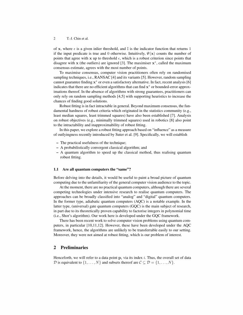
4.2 Results

Fig. 2 illustrates the results of Algorithm 1 on the data in Fig. 1. Specifically, for each

input instance, we plot in Fig. 2 the proportion of {αi}Ni=1 that are within distance

δ = 0.05 to the true {αi}Ni=1, i.e.,

1

N

N∑

i=1

I(|αi − αi| < 0.05), (27)

as a function of number of iterations M in Algorithm 1. The probabilistic lower bound

1 − 2e−2Mδ2 is also plotted as a function of M . The convergence of the approximate

influences is clearly as predicted by (26).

Fig. 3 shows the approximate influences computed using Algorithm 1 on 3 larger

input instances for homography estimation. Despite using a small number of iterations

(M ≈ 800), the inliers and outliers can be dichotomised well using the influences.

The runtimes of Algorithm 1 for the input data above are as follows:

Input data (figure) 1(a) 1(c) 1(e) 3(a) 3(c) 3(e)

Iterations (M ) 5,000 5,000 5,000 800 800 800

Runtime (s) 609 4,921 8,085 2,199 5,518 14,080

The experiments were conducted in MATLAB on a standard desktop using unoptimised

code, e.g., using fmincon to evaluate f instead of more specialised routines.

5 Quantum algorithm

We describe a quantum version of Algorithm 1 for influence computation and investi-

gate the speed-up provided.

Quantum Robust Fitting 9

0 500 1000 1500 2000 2500 3000 3500 4000 4500 5000

Number of Iterations, M

0.3

0.4

0.5

0.6

0.7

0.8

0.9

1

Pro

bab

ilit

y

1N

PNi=1 I(j,i ! ,ij < /)

1! 2e!2M/2

(a) Result for the line fitting instance in 1(a).

0 500 1000 1500 2000 2500 3000 3500 4000 4500 5000

Number of Iterations, M

0.3

0.4

0.5

0.6

0.7

0.8

0.9

1

Pro

bab

ilit

y

1N

PNi=1 I(j,i ! ,ij < /)

1! 2e!2M/2

(b) Result for the triangulation instance in 1(c).

0 500 1000 1500 2000 2500 3000 3500 4000 4500 5000

Number of Iterations, M

0.3

0.4

0.5

0.6

0.7

0.8

0.9

1

Pro

bab

ilit

y

1N

PNi=1 I(j,i ! ,ij < /)

1! 2e!2M/2

(c) Result for the homography estimation in-

stance in 1(e).

Fig. 2. Comparing approximate influences from Algorithm 1 with the true influences (13), for the

problem instances in Fig. 1. The error of the approximation (magenta) is within the probabilistic

bound (green). See Sec. 4.2 on the error metric used.

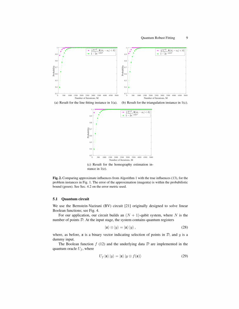
5.1 Quantum circuit

We use the Bernstein-Vazirani (BV) circuit [21] originally designed to solve linear

Boolean functions; see Fig. 4.

For our application, our circuit builds an (N + 1)-qubit system, where N is the

number of points D. At the input stage, the system contains quantum registers

|z〉 ⊗ |y〉 = |z〉 |y〉 , (28)

where, as before, z is a binary vector indicating selection of points in D, and y is a

dummy input.

The Boolean function f (12) and the underlying data D are implemented in the

quantum oracle Uf , where

Uf |z〉 |y〉 = |z〉 |y ⊗ f(z)〉 (29)

10 T.-J. Chin et al.

(a)

20 40 60 80 100 120 140 160 180 200 220

Point Index i

0

0.1

0.2

0.3

0.4

0.5

0.6

0.7

0.8

0.9

1

Influence

Threshold

(b)

(c)

50 100 150 200 250 300 350 400 450 500

Point Index i

0

0.1

0.2

0.3

0.4

0.5

0.6

0.7

0.8

0.9

1

Influence

Threshold

(d)

(e)

100 200 300 400 500 600 700

Point Index i

0

0.1

0.2

0.3

0.4

0.5

0.6

0.7

0.8

0.9

1

Influence

Threshold

(f)

Fig. 3. Large homography estimation instances, separated into inliers (blue) and outliers (red)

according to their normalised approximate influences (right column), which were computed using

Algorithm 1. Note that only about M = 800 iterations were used in Algorithm 1 to achieve these

results. Row 1 shows an instance with N = 237 correspondences; Row 2 shows an instance with

N = 516 correspondences; Row 3 shows an instance with N = 995 correspondences.

Quantum Robust Fitting 11

|z〉

|y〉

H⊗N

Uf

H⊗N

Φ4

H H

Φ1 Φ2 Φ3

Fig. 4. Quantum circuit for influence computation.

and ⊕ is bit-wise XOR. Recall that by considering only quasiconvex residual functions

(Sec. 2), f is classically solvable in polynomial time, thus its quantum equivalent Uf

will also have an efficient implementation (requiring polynomial number of quantum

gates) [22, Sec. 3.25]. Following the analysis of the well-known quantum algorithms

(e.g., Grover’s search, Shor’s factorisation algorithm), we will mainly be interested in

the number of times we need to invoke Uf (i.e., the query complexity of the algo-

rithm [23]) and not the implementation details of Uf (Sec. 5.4).

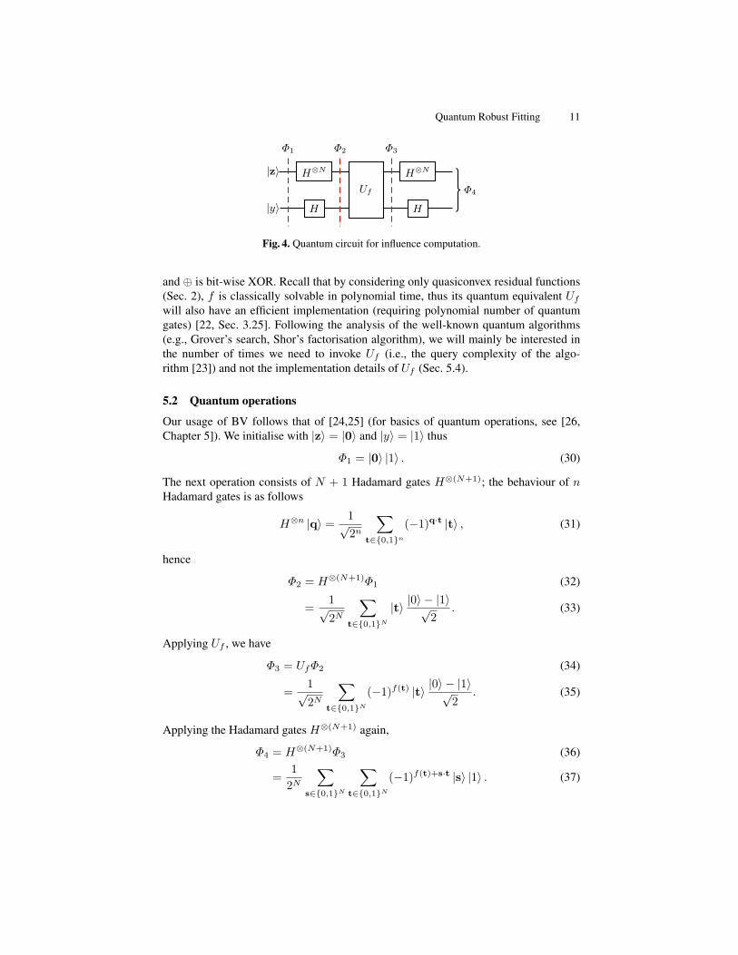
5.2 Quantum operations

Our usage of BV follows that of [24,25] (for basics of quantum operations, see [26,

Chapter 5]). We initialise with |z〉 = |0〉 and |y〉 = |1〉 thus

Φ1 = |0〉 |1〉 . (30)

The next operation consists of N + 1 Hadamard gates H⊗(N+1); the behaviour of n

Hadamard gates is as follows

H⊗n |q〉 = 1√2n

∑

t∈{0,1}n

(−1)q·t |t〉 , (31)

hence

Φ2 = H⊗(N+1)Φ1 (32)

=1√2N

∑

t∈{0,1}N

|t〉 |0〉 − |1〉√2

. (33)

Applying Uf , we have

Φ3 = UfΦ2 (34)

=1√2N

∑

t∈{0,1}N

(−1)f(t) |t〉 |0〉 − |1〉√2

. (35)

Applying the Hadamard gates H⊗(N+1) again,

Φ4 = H⊗(N+1)Φ3 (36)

=1

2N

∑

s∈{0,1}N

∑

t∈{0,1}N

(−1)f(t)+s·t |s〉 |1〉 . (37)

12 T.-J. Chin et al.

Focussing on the top-N qubits in Φ4, we have

∑

s∈{0,1}N

I(s) |s〉 , (38)

where

I(s) :=∑

t∈{0,1}N

(−1)f(t)+s·t. (39)

The significance of this result is as follows.

Theorem 1. Let s = [s1, . . . , sN ] ∈ {0, 1}N . Then

αi =∑

si=1

I(s)2. (40)

Proof. See [25, Sec. 3].

The theorem shows that the influences {αi}Ni=1 are “direct outputs” of the quantum

algorithm. However, physical laws permit us to access the information indirectly via

quantum measurements only [26, Chapter 4]. Namely, if we measure in the standard

basis, we get a realisation s with probability I(s)2. The probability of getting si = 1 is

Pr(si = 1) =∑

si=1

I(s)2 = αi. (41)

Note that the above steps involve only one “call” to Uf . However, as soon as Φ4 is

measured, the quantum state collapses and the encoded probabilities vanish.

5.3 The algorithm

Based on the setup above, running the BV algorithm once provides a single observation

of all {αi}Ni=1. This provides a basis for a quantum version of the classical Algorithm 1;

see Algorithm 2. The algorithm runs the BV algorithm M times, each time terminat-

ing with a measurement of s, to produce M realisations s[1], . . . , s[M ]. Approximate

estimates {αi}Ni=1 of the influences are then obtained by collating the results of the

quantum measurements.

5.4 Analysis

A clear difference between Algorithms 1 and 2 is the lack of an “inner loop” in the

latter. Moreover, in each (main) iteration of the quantum algorithm, the BV algorithm

is executed only once; hence, the Boolean function f is also called just once in each

iteration. The overall query complexity of Algorithm 2 is thus O(M), which is a speed-

up over Algorithm 1 by a factor of N . For example, in the case of the homography

estimation instance in Fig. 3, this represents a sizeable speed-up factor of 516.

Quantum Robust Fitting 13

Algorithm 2 Quantum algorithm to compute influence [24,25].

Require: N input data points D, inlier threshold ǫ, number of iterations M .

1: for m = 1, . . . ,M do

2: s[m] ← Run BV algorithm with D and ǫ and measure top-N qubits in standard basis.

3: end for

4: for i = 1, . . . , N do

5: αi ←1M

∑M

m=1 s[m]i .

6: end for

7: return {αi}Ni=1.

In some sense, the BV algorithm computes the influences exactly in one invocation

of f ; however, limitations placed by nature allows us to “access” the results using prob-

abilistic measurements only, thus delivering only approximate solutions. Thankfully,

the same arguments in Sec. 4.1 can be made for Algorithm 2 to yield the probabilistic

error bound (26) for the results of the quantum version.

As alluded to in Sec. 5, the computational gain is based on analysing the query

complexity of the algorithm [23], i.e., the number of times Uf needs to be invoked,

which in turn rests on the knowledge that any polynomial-time classical algorithm can

be implemented as a quantum function f efficiently, i.e., with a polynomial number

of gates (see [22, Chap. 3.25] and [26, Chap. 6]). In short, the computational analysis

presented is consistent with the literature on the analysis of quantum algorithms.

6 Conclusions and future work

We proposed one of the first quantum robust fitting algorithms and established its prac-

tical usefulness in the computer vision setting. Future work includes devising quantum

robust fitting algorithms that have better speed-up factors and tighter approximation

bounds. Implementing the algorithm on a quantum computer will also be pursued.

References

1. Hartnett, K.: Q&A with Judea Pearl: To build truly intelligent machines, teach them

cause and effect. (https://www.quantamagazine.org/to-build-truly-intelligent-machines-

teach-them-cause-and-effect-20180515/, retrieved 30 May 2020)

2. Kanatani, K., Sugaya, Y., Kanazawa, Y.: Ellipse Fitting for Computer Vision: Implementa-

tion and Applications. Synthesis Lectures on Computer Vision. Morgan & Claypool Pub-

lishers (2016)

3. Chin, T.J., Suter, D.: The maximum consensus problem: recent algorithmic advances. Syn-

thesis Lectures on Computer Vision. Morgan & Claypool Publishers, San Rafael, CA, U.S.A.

(2017)

4. Fischler, M.A., Bolles, R.C.: Random sample consensus: a paradigm for model fitting with

applications to image analysis and automated cartography. Communications of the ACM 24

(1981) 381–395

5. Raguram, R., Chum, O., Pollefeys, M., Matas, J., Frahm, J.M.: USAC: a universal frame-

work for random sample consensus. IEEE Transactions on Pattern Analysis and Machine

Intelligence 35 (2013) 2022–2038

14 T.-J. Chin et al.

6. Chin, T.J., Cai, Z., Neumann, F.: Robust fitting in computer vision: easy or hard? In: Euro-

pean Conference on Computer Vision (ECCV). (2018)

7. Bernholt, T.: Robust estimators are hard to compute. Technical Report 52, Technische

Universitat Dortmund (2005)

8. Touzmas, V., Antonante, P., Carlone, L.: Outlier-robust spatial perception: hardness, general-

purpose algorithms, and guarantees. In: IEEE/RSJ International Conference on Intelligent

Robots and Systems (IROS). (2019)

9. Suter, D., Tennakoon, R., Zhang, E., Chin, T.J., Bab-Hadiashar, A.: Monotone boolean func-

tions, feasibility/infeasibility, lp-type problems and maxcon (2020)

10. Neven, H., Rose, G., Macready, W.G.: Image recognition with an adiabatic quantum com-

puter I. Mapping to quadratic unconstrained binary optimization. arXiv:0804.4457 (2008)

11. Nguyen, N.T.T., Kenyon, G.T.: Image classification using quantum inference on the D-Wave

2X. arXiv:1905.13215 (2019)

12. Golyanik, V., Theobalt, C.: A quantum computational approach to correspondence problems

on point sets. In: IEEE Computer Society Conference on Computer Vision and Pattern

Recognition (CVPR). (2020)

13. Kahl, F., Hartley, R.: Multiple-view geometry under the l∞-norm. IEEE Transactions on

Pattern Analysis and Machine Intelligence 30 (2008) 1603–1617

14. Eppstein, D.: Quasiconvex programming. Combinatorial and Computational Geometry 25

(2005)

15. Chin, T.J., Purkait, P., Eriksson, A., Suter, D.: Efficient globally optimal consensus maximi-

sation with tree search. In: IEEE Computer Society Conference on Computer Vision and

Pattern Recognition (CVPR). (2015)

16. Cheney, E.W.: Introduction to Approximation Theory. McGraw-Hill (1966)

17. Chum, O., Matas, J.: Matching with PROSAC - progressive sample consensus. In: IEEE

Computer Society Conference on Computer Vision and Pattern Recognition (CVPR). (2005)

18. Amenta, N., Bern, M., Eppstein, D.: Optimal point placement for mesh smoothing. J. Algo-

rithms 30 (1999) 302–322

19. Matousek, J., Sharir, M., Welzl, E.: A subexponential bound for linear programming. Algo-

rithmica 16 (1996) 498–516

20. (https://en.wikipedia.org/wiki/Hoeffding%27s_inequality)

21. Bernstein, E., Vazirani, U.: Quantum complexity theory. SIAM J. Comput. 26 (1997) 1411–

1473

22. Nielsen, M.A., Chuang, I.L.: Quantum computation and quantum information. Cambridge

University Press (2010)

23. Ambainis, A.: Understanding quantum algorithms via query complexity. In: International

Congress of Mathematics. Volume 4. (2018) 3283–3304

24. Floess, D.F., Andersson, E., Hillery, M.: Quantum algorithms for testing Boolean functions.

Math. Struc. Comput. Sci. 23 (2013) 386–398

25. Li, H., Yang, L.: A quantum algorithm for approximating the influences of boolean functions

and its applications. Quantum Information Processing 14 (2015) 1787–1797

26. Rieffel, E., Polak, W.: Quantum computing: a gentle introduction. The MIT Press (2014)