Cowles Foundation for Research in Economics at Yale University

Cowles Foundation Discussion Paper No. 1821

Princeton University, Department of Economics Economic Theory Center Working Paper No. 023-2011

ROBUST PREDICTIONS IN GAMES WITH

INCOMPLETE INFORMATION

September 2011

Dirk Bergemann

Yale University - Cowles Foundation - Department of Economics

Stephen Morris

Princeton University - Department of Economics

Electronic copy available at: http://ssrn.com/abstract=1933781

Robust Predictions

in

Games with Incomplete Information�

Dirk Bergemanny Stephen Morrisz

September 26, 2011

Abstract

We analyze games of incomplete information and o¤er equilibrium predictions which are valid for all possible

private information structures that the agents may have. Our characterization of these robust predictions relies

on an epistemic result which establishes a relationship between the set of Bayes Nash equilibria and the set of

Bayes correlated equilibria.

We completely characterize the set of Bayes correlated equilibria in a class of games with quadratic payo¤s

and normally distributed uncertainty in terms of restrictions on the �rst and second moments of the equilibrium

action-state distribution. We derive exact bounds on how prior information of the analyst re�nes the set of

equilibrium distribution. As an application, we obtain new results regarding the optimal information sharing

policy of �rms under demand uncertainty.

Finally, we reverse the perspective and investigate the identi�cation problem under concerns for robustness

to private information. We show how the presence of private information leads to partial rather than complete

identi�cation of the structural parameters of the game. As a prominent example we analyze the canonical problem

of demand and supply identi�cation.

Jel Classification: C72, C73, D43, D83.

Keywords: Incomplete Information, Correlated Equilibrium, Robustness to Private Information, Moments Re-

strictions, Identi�cation, Information Bounds.

�We acknowledge �nancial support through NSF Grant SES 0851200. We bene�tted from comments of Steve Berry, Vincent Crawford,

Phil Haile, Marc Henry, Arthur Lewbel, Larry Samuelson, and Elie Tamer, and research assistance from Brian Baisa and Aron Tobias.

We would like to thank seminar audiences at Boston College, the Collegio Carlo Alberto, Ecole Polytechnique, European University

Institute, HEC, Microsoft Research, Northwestern University, the Paris School of Economics, Stanford University and the University of

Colorado for stimulating conversations; and we thank David McAdams for his discussion of this work at the 2011 North American Winter

Meetings of the Econometric Society in Denver.yDepartment of Economics, Yale University, New Haven, CT 06520, U.S.A., dirk.bergemann@yale.edu.zDepartment of Economics, Princeton University, Princeton, NJ 08544, U.S.A. smorris@princeton.edu

1

Electronic copy available at: http://ssrn.com/abstract=1933781

1 Introduction

In games of incomplete information, the private information of each agent typically induces posterior beliefs

about some payo¤ state, and a posterior belief about the beliefs of the other agents. In turn, the private

information of the agent, the type in the language of Bayesian games, in�uences the optimal strategies of the

agents, and ultimately the equilibrium distribution over actions and states. The posterior belief about the

payo¤ state represents the knowledge about the payo¤ environment that the player is facing, whereas the

posterior belief about the beliefs of the other agents represents the knowledge about the belief environment

that the player is facing. The objective of this paper is to obtain equilibrium predictions for a given

payo¤ environment which are independent of - and in that sense robust to - the speci�cation of the belief

environment.

We de�ne the payo¤environment as the complete description of the agents�preferences and the common

prior over the payo¤states. The fundamental uncertainty about the set of feasible payo¤s is thus completely

described by the common prior over the payo¤ states, which we also refer to as a fundamental state. We

de�ne the belief environment by a complete description of the common prior type space over and above

the information contained in the common prior distribution of the payo¤ states. The belief environment

then describes a potentially rich type space which is only subject to the constraint that the marginal

distribution over the fundamental variable coincides with the common prior over payo¤ states. A pair

of payo¤ environment and belief environment form a standard Bayesian game. Yet, for a given payo¤

environment, there are many belief environments, and each distinct belief environment may lead to distinct

equilibrium distribution over outcomes, namely actions and fundamentals.

The objective of the paper is to describe the equilibrium implications of the �payo¤ environment�for

all possible �belief environments�relative to the given payo¤ environment. Consequently, we refer to the

(partial) characterization of the equilibrium outcomes that are independent of the belief environment as

robust predictions. We examine these issues in a tractable class of games with a continuum of players,

symmetric payo¤ functions, and linear best response functions. A possible route towards a comprehen-

sive description of the equilibrium implications stemming from the payo¤ environment alone, would be

an exhaustive analysis of all Bayes Nash equilibria of all belief environments which are associated with

a given payo¤ environment. Here we shall not pursue this direct approach. Instead we shall use a re-

lated equilibrium notion, namely the notion of Bayes correlated equilibrium to obtain a comprehensive

characterization. We begin with an epistemic result that establishes the equivalence between the class of

Bayes Nash equilibrium distributions for all possible belief environments and the class of Bayes correlated

equilibrium distributions. This result is a natural extension of a seminal result by Aumann (1987). In

games with complete information about the payo¤ environment, he establishes the equivalence between

2

the set of Bayes Nash equilibria and the set of correlated equilibria. We present the epistemic result for

the class of games with a continuum of agent and symmetric payo¤ functions, and show that the insights

of Aumann (1987) generalizes naturally to this class of games with incomplete information.

Subsequently we use the epistemic result to provide a complete characterization of the Bayes correlated

equilibria in the class of games with quadratic payo¤s. With quadratic games, the best response function

of each agent is a linear function and in consequence the conditional expectations of the agents are linked

through linear conditions which in turn permits an explicit construction of the equilibrium sets. The

class of quadratic games has featured prominently in many recent contributions to games of incomplete

information, for example the analysis of rational expectations in competitive markets by Guesnerie (1992),

the analysis of the beauty contest by Morris and Shin (2002) and the equilibrium use of information by

Angeletos and Pavan (2007). We o¤er a characterization of the equilibrium outcomes in terms of the

moments of the equilibrium distributions. In the class of quadratic games, we show that the expected

mean is constant across all equilibria and provide sharp inequalities on the variance-covariance of the joint

outcome state distributions. If the underlying uncertainty about the payo¤ state and the equilibrium

distribution itself is normally distributed then the characterization of the equilibrium is completely given

by the �rst and second moments. If the distribution of uncertainty or the equilibrium distribution itself

is not normally distributed, then the characterization of �rst and second moments remains valid, but of

course it is not a complete characterization in the sense that the determination of the higher moments is

incomplete.

In a companion paper, Bergemann and Morris (2011), we report the de�nition of Bayes correlated

equilibrium and the relevant epistemic results in a canonical game theoretic framework with a �nite number

of agents, a �nite set of pure action and a �nite set of payo¤ relevant states. We also relate this to the

prior literature on incomplete information correlated equilibrium, notably Forges (1993). In the present

paper, the analysis will be con�ned to an environment with quadratic and symmetric payo¤ functions, a

continuum of agents and normally distributed uncertainty about the common payo¤ relevant state. This

tractable class of models enables us to o¤er robust predictions in terms of restrictions on the �rst and

second moments of the joint distribution over actions and state. By contrast, in the companion paper, we

present the de�nition of the Bayes correlated equilibrium in a canonical game theoretic framework. Still, the

separation between payo¤ and belief environment enables us to ask how changes in the belief environment

a¤ect the equilibrium set for a given and �xed payo¤ environment. We introduce a natural partial order

on information structures that captures when one information structure contains more information than

another. This partial order is a variation on a many player generalization of the ordering of Blackwell

(1953) introduced by Lehrer, Rosenberg, and Shmaya (2010), (2011) and there we establish that the set of

3

Bayes correlated equilibria shrinks as the informativeness of the information structure increases.

The relationship between the Bayes Nash equilibrium and the Bayes correlated equilibrium is also useful

to examine the impact of the information structure on the welfare of the agents. The compact representation

of the Bayes correlated equilibria allows us to assess the private and/or social welfare across the entire set of

equilibria and we illustrate this in the context of information sharing among �rms. The issue is to whether

competing �rms have an incentive to share information in an uncertain environment. A striking result by

Clarke (1983) was the �nding that �rms, when facing uncertainty about a common parameter of demand,

will never �nd it optimal to share information. The present analysis of the Bayes correlated equilibrium

allows us to modify this insight - implicitly by allowing for richer information structures than previously

considered - and we �nd that the Bayes correlated equilibrium that maximizes the private welfare of the

�rms is not necessarily obtained with zero or full information disclosure.

The initial equivalence result between Bayes correlated and Bayes Nash equilibrium relied on very

weak assumptions about the belief environment of the agents. In particular, we allowed for the possibility

that the agents may have no additional information beyond the common prior about the payo¤ state.

Yet, in some circumstances the agents may be commonly known to have some given prior information, or

background information. Consequently, we then analyze how a lower bound on either the public or the

private information of the agents, can be used to further re�ne the robust predictions and impose additional

moment restrictions on the equilibrium distribution.

The payo¤ environment is speci�ed by the (ex-post) observable outcomes, the actions and the payo¤

state. By contrast, the elements of the belief environment, the beliefs of the agents, the beliefs over the

beliefs of the agents, etc. are rarely directly observed or inferred from the revealed choices of the agents.

The absence of the observability (via revealed preference) of the belief environment then constitutes a

separate reason to be skeptical towards an analysis which relies on very speci�c and detailed assumptions

about the belief environment. (In separate work, Bergemann, Morris, and Takahashi (2010) ask what can

be learned about agents�possibly interdependent preferences by observing how they behave in strategic

environments. As they are interested in identifying when two types are strategically distinguishable in the

sense that they are guaranteed to behave di¤erently in some �nite game, their framework is di¤erent from

the current one, as here we consider a given game rather than quantifying over all games.)

Finally, we reverse the perspective of our analysis and consider the issue of identi�cation rather than the

issue of prediction. In other words, we are asking whether the observable data, namely actions and payo¤

state, can identify the structural parameters of the payo¤ functions, and thus of the game, without stringent

assumptions on the belief environment. The question of identi�cation is to ask whether the observable

data imposes restrictions on the unobservable structural parameters of the game given the equilibrium

4

hypothesis. Similarly to the problem of robust equilibrium prediction, the question of robust identi�cation

then is which restrictions are common to all possible belief environments given a speci�c payo¤environment.

In the context of the quadratic payo¤s that we study, we �nd that the robust identi�cation does allow us to

identify the sign of some interaction parameters, but will leave other parameters, in particular whether the

agents are playing a game of strategic substitutes or complements, unidenti�ed, even in terms of the sign of

the interaction. The identi�cation results here, in particular the contrast between Bayes Nash equilibrium

and Bayes correlated equilibrium, are related to, but distinct from the results presented in Aradillas-Lopez

and Tamer (2008). In their analysis of an entry game with incomplete information, they document the loss

in identi�cation power that arises with a more permissive solution concept, i.e. level k-rationalizability.

As we compare Bayes Nash and correlated equilibrium, we show that the lack of identi�cation is not

necessarily due to the lack of a common prior, as associated with rationalizability, but rather the richness

of the possible private information structures (but all with a common prior).

In recent years, the concern for a robust equilibrium analysis in games of incomplete information has

been articulated in many ways. In mechanism design, where the rules of the games can be chosen to

have favorable robustness properties, a number of positive results have been obtained. Dasgupta and

Maskin (2000), Bergemann and Välimäki (2002) and Bergemann and Morris (2005), among others, show

that the e¢ cient social allocation can be implemented in an ex-post equilibrium and hence in Bayes Nash

equilibrium for all type spaces, with or without a common prior.1 But in �given�rather than �designed�

games, such strong robustness results seem out of reach for most classes of games. In particular, many

Bayesian games simply do not have ex post or dominant strategy equilibria. In the absence of such

global robustness results, a natural �rst step is then to investigate the robustness of the Bayes Nash

equilibrium to a small perturbation of the information structure. For example, Kajii and Morris (1997)

consider a Nash equilibrium of a complete information game and say that the Nash equilibrium is robust

to incomplete information if every incomplete information game with payo¤s almost always given by the

complete information game has an equilibrium which generates behavior close to the Nash equilibrium. In

this paper, we take a di¤erent approach and use the dichotomy between the payo¤ environment and the

belief environment to analyze the equilibrium behavior in a given payo¤ environment while allowing for

any arbitrary, but common prior, type space, as long as it is consistent with the given common prior of

the payo¤ type space. In the current contribution, we trace out the Bayes Nash equilibria associated with

all possible information structures. A related literature seeks to identify the best information structure

consistent with the given common prior over payo¤ types. For example, Bergemann and Pesendorfer (2007)

1Jehiel and Moldovanu (2001) and Jehiel, Moldovanu, Meyer-Ter-Vehn, and Zame (2006) demonstrate the limits of these

results by considering multi-dimensional payo¤ types.

5

characterizes the revenue-maximizing information structure in an auction with many bidders. Similarly,

in a class of sender-receiver games, Kamenica and Gentzkow (2010) derive the sender-optimal information

structure.

Chwe (2006) discusses the role of statistical information in single-agent and multi-agent decision prob-

lems. In a series of related settings, he argues that the correlation between the revealed choice of an agent,

referred to as incentive compatibility, and a random variable, not controlled by the agent, allows us an

analyst to infer the nature of the payo¤ interaction between the agent�s choice and the random variable.

For example, in 2 � 2 games, observing the signed covariance in the actions is su¢ cient to identify purestrategy Nash equilibria. In the context of a two player game with quadratic payo¤s and complete informa-

tion, he shows that the sign of the covariance of the agents�actions can be predicted across all correlated

equilibria.

The remainder of the paper is organized as follows. Section 2 de�nes the relevant solution concepts

and establishes the epistemic result which relates the set of Bayes Nash equilibria to the set of Bayes

correlated equilibria. Beginning with Section 3, we con�ne our attention to a class of quadratic games

with normally distributed uncertainty about the payo¤ state. Section 4 reviews the standard approach

to games with incomplete information and analyses the Bayes Nash equilibria under a bivariate belief

environment in which each agent receives a private and a public signal about the payo¤ state. Section 5

begins with the analysis of the Bayes correlated equilibrium and we present a complete description of the

equilibrium set in terms of moment restrictions on the joint equilibrium distribution. We then establish the

link between the set of Bayes correlated equilibria and the set Bayes Nash equilibrium under the bivariate

belief environment. In Section 6 we analyze how prior information about the belief environment can further

restrict the equilibrium predictions. In Section 7, we turn from prediction to the issue of identi�cation. We

ask how much we can learn from the observable actions and payo¤ states about the structural parameters

of the game. Here we consider both the case of observable individual actions as well as observable aggregate

actions. With only aggregate actions observable, we consider the possibility of robust identi�cation within

the context of the classic demand and supply identi�cation problem. Section 8 discusses some possible

extensions and o¤ers concluding remarks. The Appendix collects some of the proofs from the main body

of the text.

6

2 Set-Up

We �rst de�ne the solution concept of Bayes correlated equilibrium. We then relate the notion of Bayes

correlated equilibrium to robust equilibrium predictions in a class of continuum player games with symmet-

ric payo¤. In the companion paper, Bergemann and Morris (2011), we develop this solution concept and

its relationship to robust predictions in canonical �nite player and �nite action games. In the companion

paper, we also show how the results there can be adapted and re�ned �rst to symmetric payo¤s and then

to the continuum of agents and continuum of actions analyzed here.

Payo¤ Environment There is a continuum of players and an individual player is indexed by i 2 [0; 1].Each player chooses an action a 2 R. There will then be a realized population action distribution

h 2 �(R). There is a payo¤ state � 2 �. All players have the same payo¤ function u : R��(R)��! R,

where u (a; h; �) is a player�s payo¤ if she chooses action a, the population action distribution is h and the

state is �. There is a prior distribution 2 �(�). A payo¤ environment is thus parameterized by (u; ).We also refer to (u; ) as the "basic game" as 2 �(�) only speci�es the common prior distribution overthe payo¤ state � 2 � whereas it does not specify the private information the agents may have access to.

Belief Environment Each player will observe a signal (or realize a type) t 2 T . In each state of the

world � 2 �, there will be a realized distribution of signals g 2 �(T ) drawn according to a distributionk 2 �(� (T )). Let � : � ! �(� (T )) give the distribution over signal distributions. Thus the belief

environment, or alternatively an �information structure�, is parameterized by (T; �).

Bayes Correlated Equilibrium We will be interested in probability distributions � 2 �(� (R)��)with the interpretation that � is the joint distribution of the population action distribution h and the state

�. For any such �, we write b� for the induced probability distribution on R��(R)�� if (h; �) 2 �(R)��are drawn according to � and there is then a conditionally independent draw of a 2 R according to h. Foreach a 2 R, we write b� (�ja) for the probability on �(R) � � conditional on a (we will write as if it is

uniquely de�ned).

De�nition 1 (Bayes Correlated Equilibrium )

A probability distribution � 2 �(� (R)��) is a Bayes correlated equilibrium (BCE) of (u; ) if

Eb�(�ja)u (a; h; �) � Eb�(�ja)u �a0; h; �� (1)

for each a and a0; and

marg�� = :

7

In our de�nition of Bayes correlated equilibrium, the types Ti are implicit in the sense that the proba-

bility distribution � will induce a belief over actions and beliefs of the other players. Thus, our de�nition

extends the notion of a correlated equilibrium in Aumann (1987) to an environment with uncertain payo¤s,

represented by the state of the world �. We introduce the language of types later on when we consider

games in which the players are known to have private information about the state of world, which is

encoded in the types.

In our companion paper, Bergemann and Morris (2011), the notion of Bayes correlated equilibrium is

de�ned somewhat more generally as a joint distribution over action, states and types, i.e. as a joint distri-

bution � 2 �(A��� T ). In the language of the more general notion o¤ered there, the Bayes correlatedequilibrium de�ned here is the Bayes correlated information with the �null information structure�, i.e. the

case in which the agents are not assumed a priori to have access to a speci�c information structure (T; �).

Here, we choose this minimal notion of a Bayes correlated equilibrium to obtain robust predictions for an

observer who only knows the payo¤ environment but has �null�information about the belief environment

of the game. But, just as in the companion paper, Bergemann and Morris (2011), we can analyze the

impact of private information on the size of the Bayes correlated equilibrium set. In fact in Section 6, we

analyze how prior knowledge of the belief environment can re�ne the set of equilibrium predictions. We

maintain our restriction to normally distributed uncertainty, now normally distributed types, to obtain

explicit descriptions of the resulting restriction on the equilibrium set. By contrast, in Bergemann and

Morris (2011), we allow for general information structures and derive a many player generalization of the

ordering of Blackwell (1953) as a necessary and su¢ cient conditions to order the set of Bayes correlated

equilibrium. However, within this general environment, we do not obtain an explicit and compact descrip-

tion of the equilibrium set in terms of the �rst and second moments of the equilibrium distributions, as we

do in the present analysis.

The general notion of Bayes correlated information also facilitates the discussion of the relationships

between the notion of Bayes correlated equilibrium, and related, but distinct notions of correlated equilib-

rium in games of incomplete information, most notably in the work of Forges (1993), which is titled and

identi�es ��ve legitimate de�nitions of correlated equilibrium in games with incomplete information�. We

refer to the reader to the companion paper, Bergemann and Morris (2011) for a detailed discussion and

comparison.

Bayes Nash Equilibrium The payo¤ environment (u; ) and the belief environment (T; �) together

de�ne a game of incomplete information ((u; ) ; (T; �)). A symmetric strategy in the game is then

de�ned by � : T ! �(R). The interpretation is that � (t) is the realized distribution of actions among

those players observing signal t (i.e., we are "assuming the law of large numbers" on the continuum). A

8

distribution of signals g 2 �(T ) and � 2 � induce a probability distribution g � � 2 �(R). The prior

2 �(�) and signal distribution � : �! �(T ) induce a probability distribution � � 2 �(� (T )��).As before, write [ � � for the probability distribution on T ��(T ) � � if (g; �) 2 �(T ) � � are drawn

according to � � and there is then a conditionally independent draw of t 2 T according to the realizedg 2 �(T ). For each t 2 T , we write [ � � (�jt) for the probability on �(T )�� conditional on t (we willwrite as if it is uniquely de�ned).

De�nition 2 (Bayes Nash Equilibrium)

A strategy � 2 � is a Bayes Nash equilibrium (BNE) of ((u; ) ; (T; �)) if

E[ ��(�jt)u (a; g � �; �) � E[ ��(�jt)u�a0; g � �; �

�;

for all t 2 T , a in the support of � (� jt) and a0 2 R.

Let � � � � be the probability distribution on �(� (R)��) induced if (g; �) 2 �(T )�� are drawnaccording to � � and h 2 �(R) is set equal to g � �.

De�nition 3 (Bayes Nash Equilibrium Distribution)

A probability distribution � 2 �(� (R)��) is a BNE action state distribution of ((u; ) ; (T; �)) if thereexists a BNE � of ((u; ) ; (T; �)) such that � = � � � �.

Epistemic Result We are now in a position to relate the Bayes correlated equilibria with the Bayes

Nash equilibria.

Proposition 1

A probability distribution � 2 �(� (R)��) is a Bayes correlated equilibrium of (u; ) if and only if it is

a BNE action state distribution ((u; ) ; (T; �)) for some information structure (T; �).

Proof. Suppose that � is a BCE of (u; ). Let T = R, let � : � ! �(T ) be set equal to the

conditional probability � : �! �(R) and let � be the "truth-telling" strategy with type a choosing action

a with probability 1. Now

E[ ��(�ja)u�a0; g � �; �

�= Eb�(�ja)u �a0; h; ��

by construction and the BCE equilibrium conditions imply the BNE equilibrium conditions.

Suppose that � is a BNE of ((u; ) ; (T; �)) and so

E[ ��(�jt)u (a; g � �; �) � E[ ��(�jt)u�a0; g � �; �

�(2)

9

for all t 2 T , a in the support of � (� jt) and a0 2 R. Now E[ ��(�jt)u (a0; g � �; �) is a function of t. The

expectation of this expectation conditional on a being drawn under strategy � is

E\ ����(�ja)u�a0; g � �; �

�and thus taking the expectation of both sides of (2) establishes that � � � � is a BCE.

Aumann (1987) establishes the relation between Nash equilibria and correlated equilibria in games with

complete information. In the companion paper, Bergemann and Morris (2011), we establish the relevant

epistemic results for canonical game theoretic environments in more detail.

3 Environment with Quadratic Payo¤s and Normal Uncertainty

For the remainder of this paper, we consider a quadratic and symmetric model of interaction. There is

a continuum of agents, i 2 [0; 1]. The individual action is denoted by ai 2 R and the average action isdenoted by A 2 R:

A ,Ziaidi.

The payo¤ of agent i is denoted by ui (ai; A; �) and depends on the individual action ai, the average action

A and the payo¤ state � 2 R. The payo¤s are quadratic and symmetric across agents and given by:

ui (ai; A; �) ,

0BB@�a

�A

��

1CCA00BB@

ai

A

�

1CCA+0BB@

ai

A

�

1CCA00BB@

a aA a�

aA A A�

a� A� �

1CCA0BB@

ai

A

�

1CCA : (3)

The vector � = (�a; �A; ��) represents the linear returns and the matrix � =� ijrepresents the inter-

action structure of the game, together � and � completely describe the payo¤s of the agents. The entries

in the interaction matrix � are uniformly denoted by . The parameters with a single subscript, namely

a; A; �, refer the diagonal entries in the interaction matrix �. We assume that the payo¤s are concave

in the own action:

a < 0;

and that the interaction of the individual action and the average action (the �indirect e¤ect�) is bounded

by the own action (the �direct e¤ect�):

� aA= a < 1 , a + aA < 0. (4)

The concavity and the moderate interaction jointly imply that the complete information game has a

unique and bounded Nash equilibrium. The game displays strategic complementarity if aA > 0 and

10

strategic substitutes if aA < 0. We assume that the informational externality a� is nonzero to have the

fundamental, i.e. the payo¤ state �, matter. The entries in the interaction matrix � which do not refer to

the individual action ai, i.e. the entries in the lower submatrix of �, namely24 A A�

A� �

35 (5)

are not relevant for the determination of either the Bayes Nash or the Bayes correlated equilibrium. These

entries may gain relevance if we were to pursue a welfare analysis, where the aggregate behavior per se

would in�uence the evaluation of an equilibrium or a policy intervention (see for example Angeletos and

Pavan (2009)). As this is not the subject of the paper, the entries in the lower submatrix (5) do not matter

for us, and can be uniformly set to zero.

The payo¤ state, or the state of the world, � is distributed normally with

� � N���; �

2�

�.

The quadratic environment encompasses a wide class of interesting economic environment. The following

two applications are prominent examples and we shall return to them throughout the paper to illustrate

some of the results.

Example 1 (Beauty Contest) In Morris and Shin (2002), a continuum of agents, i 2 [0; 1], have tochoose an action under incomplete information about the state of the world �. Each agent i has a payo¤

function given by:

ui (ai; A; �) = � (1� r) (ai � �)2 � r (ai �A)2 .

The weight r re�ects concern for the average action A taken in the population. Morris and Shin (2002)

analyze the Bayes Nash equilibrium in which each agent i has access to a private (idiosyncratic) signal

and a public (common) signal of the world. In terms of our notation, the beauty contest model set a =

�1, aA = r 2 (0; 1) and a� = (1� r). Angeletos and Pavan (2007) generalize the analysis of BayesNash equilibrium under this bivariate information structure for the general class of quadratic environments

de�ned above by (3).

Example 2 (Competitive Market) Guesnerie (1992) o¤er an analysis of the stability of the competitive

equilibrium by considering a continuum of producers with a quadratic cost of production and a linear inverse

demand function with either cost or demand uncertainty. In terms of our notation, the cost of production

of the individual �rm is described by c (ai) = ��aai � a�ai� � aa2i if there is common cost uncertainty,

and by c (ai) = ��aai� aa2i if there is demand uncertainty. In turn, the inverse demand function is givenby p (A) = aAA if there is cost uncertainty, and p (A) = a�� + aAA if there is demand uncertainty,

where the state � now determines the intercept of the inverse demand.

11

4 Bayes Nash Equilibrium

We initially report the standard approach to analyze games of incomplete information. Namely, we start

with the game of incomplete information, which includes the basic game and a speci�c type space. Here,

the type space consists of a two-dimensional signal that each agent receives. In the �rst dimension, the

signal is privately observed and idiosyncratic to the agent, whereas in the second dimension, the signal is

publicly observed and common to all the agents. In either dimension, the signal is normally distributed and

centered around the true state of the world �. In this class of normally distributed signals, a speci�c type

space is determined by the variance of the noise along each dimension of the signal. For a given variance-

covariance matrix, and hence for a given type space, we then analyze the Bayes Nash equilibrium/a of

the basic game. Now, the type space, as parametrized by the variance of the noise, naturally belongs to

a class of possible private information environments and hence type spaces, namely the class of normally

distributed bivariate signal structures. In the process of the analysis, we shall observe that the equilibrium

behavior across this class of normally distributed information environments displays common features. We

shall then proceed to analyze the basic game with the notion of Bayes Correlated equilibrium and establish

which predictions are robust across all of the private information environments, independent of the speci�c

bivariate and normal type space to be considered now.

Accordingly, we consider the following bivariate normal information structure. Each agent i is observing

a private and a public noisy signal of the true state of the world �. The private signal xi, observed only

by agent i, is de�ned by:

xi = � + "i; (6)

and the public signal, common and commonly observed by all the agents is de�ned by:

y = � + ". (7)

The random variables "i and " are normally distributed with zero mean and variance given by �2x and �2y,

respectively; moreover "i and " are independently distributed, with respect to each other and the state �.

This model of bivariate normally distributed signals appears frequently in games of incomplete information,

see Morris and Shin (2002) and Angeletos and Pavan (2007) among many others. It is at times convenient

to express the variance of the random variables in terms of the precision:

�x , ��2x ; �y , ��2y ; and ��2 , ��2y + ��2x + ��2� ;

we refer to the vector � with

� , (�x; �y) ,

as the information structure of the game.

12

A special case of the noisy environment is the environment with zero noise. In this environment, the

complete information environment, each agent observes the state of the world � without noise. We begin

the equilibrium analysis with the complete information environment. Given the payo¤ environment, the

best response of agent i is given by

ai = ��a + a�� + aAA

a.

The best response re�ects the, possibly con�icting, objectives that agent i faces. The quadratic payo¤

function induces each agent to solve a prediction-like problem in which he wishes to match with his action,

with the state � and the average action A. The interaction parameters, the indirect e¤ects a� and aA,

determine the weight that each component receives in the deliberation of the agent, and the direct e¤ect

a; determines the overall responsiveness to state � and average action A. If there is zero strategic

interaction, or aA = 0, then each agent faces a pure prediction problem. Now, it follows that the resulting

Nash equilibrium strategy is given by:

a� (�) , � �a a + aA

� a� a + aA

�. (8)

Given the earlier assumptions on individual and aggregate concavity of the payo¤ function, namely a < 0

and aA+ a < 0, it follows that the symmetric strategy a� (�) ; given any realization �, is the unique Nash

equilibrium of the game with complete information. In fact, a� (�) is also the unique correlated equilibrium

of the game; Neyman (1997) gives an elegant argument.

Next, we analyze the game with incomplete information, where each agent receives a bivariate noisy

signal (xi; y). In particular, we shall compare how responsive the strategy of each agent is to the underlying

state of the world relative to the responsiveness in the game with complete information. To this end,

we shall refer to the terms in equilibrium strategy (8), ��a= ( a + aA) and � a�= ( a + aA), as theequilibrium intercept and the equilibrium slope, respectively.

In the game with incomplete information, agent i receives a pair of signals, xi and y, generated by the

information structure (6) and (7). The prediction problem now becomes more di¢ cult for the agent. First,

he does not observe the state �, but rather he receives some noisy signals, xi and y, of �. Second, since he

does not observe the other agents�signals either, he can only form an expectation about their actions, but

again has to rely on the signals xi and y to form the conditional expectation. The best response function

of agent i then requires that action a is justi�ed by the conditional expectation, given xi and y:

ai = ��a + a�E [� jxi; y ] + aAE [A jxi; y ]

a.

In this linear quadratic environment with normal distributions, we conjecture that the equilibrium strategy

is given by a function linear in the signals xi and y:

a (xi; y) = �0 + �xxi + �yy. (9)

13

The equilibrium is then identi�ed by the linear coe¢ cients �0; �x; �y; which we expect to depend on the

interaction matrix � and the information structure � .

Proposition 2 (Linear Bayes Nash Equilibrium)

The unique Bayes Nash equilibrium is a linear equilibrium:

a (x; y) = ��0 + ��xx+ �

�yy

with the coe¢ cients given by:

��0 = ��a

a + aA� a a + aA

��2� a���

aA��2x + a�

�2 ; (10)

��x = � a��

�2x

aA��2x + a�

�2 ; (11)

��y = � a

a + aA

a���2y

aA��2x + a�

�2 : (12)

The derivation of the linear equilibrium strategy already appeared in many contexts, e.g., in Morris

and Shin (2002) for the beauty contest model, and for the present general environment, in Angeletos and

Pavan (2007). The Bayes Nash equilibrium shares the uniqueness property with the Nash equilibrium, its

complete information counterpart. We observe that the linear coe¢ cient ��x and ��y display the following

relationship:��y��x

=�2x�2y

a a + aA

. (13)

Thus, if there is zero strategic interaction, or aA = 0, then the signals xi and y receive weights proportional

to the precision of the signals. The fact that xi is a private signal and y is a public signal does not matter

in the absence of strategic interaction, all that matters is the ability of the signal to predict the state of

the world. By contrast, if there is strategic interaction, aA 6= 0, then the relative weights also re�ect

the informativeness of the signal with respect to the average action. Thus if the game displays strategic

complements, aA > 0, then the public signal y receives a larger weight. The commonality of the public

signal across agents means that their decision is responding to the public signal at the same rate, and hence

in equilibrium the public signal is more informative about the average action than the private signal. By

contrast, if the game displays strategic substitutability, aA < 0, then each agent would like to move away

from the average, and hence places a smaller weight on the public signal y, even though it still contains

information about the underlying state of the world.

Now, if we compare the equilibrium strategies under complete and incomplete information, (8) and

(9), we �nd that in the incomplete information environment, each agent still responds to the state of the

14

world �, but his response to � is noisy as both xi and y are noisy realizations of �, but centered around

�: xi = � + "i and y = � + ". Now, given that the best response, and hence the equilibrium strategy, of

each agent is linear in the expectation of �, the variation in the action is �explained�by the variation in

the true state, or more generally in the expectation of the true state. Thus the ��ows�of the action have

to be balanced by the ��ows�of the underlying state �. But across all of the information structures, the

distribution of the state � remains the same, which suggests that the expected �ows have to stay constant

across the information structures.

Proposition 3 (Attenuation)

The mean action in equilibrium is:

E [a] = ��0 + ��x�� + �

�y�� = �

�a + a��� a + aA

;

and the sum of the weights, ��x + ��y, is:

����x + ��y�� = ����� a� a + aA

���� 1�

a��2�

a��2 + aA�

�2x

!������ a� a + aA

���� .Thus, the average action in equilibrium, E [a], is in fact independent of the information structure � . In

addition, we �nd that the linear coe¢ cients of the equilibrium strategy under incomplete information are

(weakly) less responsive to the true state � than under complete information. In particular, the sum of the

weights is strictly increasing in the precision of the noisy signals xi and y. The equilibrium response to the

state of the world � is diluted by the noisy signals, that is the response is attenuated. But as the expected

�ows have to be balanced, the residual is always picked up by the intercept of the equilibrium response.

Now, if we ask how the joint distribution of the Bayes Nash equilibrium vary with the information

structure, then Proposition 3 established that it is su¢ cient to consider the higher moments of the equi-

librium distribution. But given the normality of the equilibrium distribution, it follows that it is su¢ cient

to consider the second moments, that is the variance-covariance matrix. The variance-covariance matrix

of the equilibrium joint distribution over individual actions ai; aj , and state � is given by:

�ai;aj ;� =

2664�2a �a�

2a �a��a��

�a�2a �2a �a��a��

�a��a�� �a��a�� �2�

3775 : (14)

We denote the correlation coe¢ cient between action ai and aj shorthand by �a rather than �aa. Above,

we describe the equilibrium joint distribution in terms of (ai; aj ; �), but alternatively we can describe it,

after replacing the individual action aj by the average action A, through the triple (ai; A; �). After all,

the covariance between the individual, but symmetrically distributed, actions ai and aj , given by �a�2a

15

has to be equal to the variance of the average action, or �2A = �a�2a. Similarly, the covariance between

the individual action and the average action has to be equal to the covariance of any two, symmetric,

individual action pro�les, or �aA�a�A = �a�2a. Likewise, the covariance between the individual (but

symmetric) action ai and the state � has to equal to the covariance between the average action and the

state �, or or �a��a�� = �A��A��. The variance-covariance matrix of the equilibrium joint distribution

over individual actions ai; A and state � is given by:

�ai;A;� =

2664�2a �a�

2a �a��a��

�a�2a �a�

2a �a��a��

�a��a�� �a��a�� �2�

3775 :Now, given the characterization of the unique Bayes Nash equilibrium in Proposition 2 above, we can

express either of the variance-covariance matrices in terms of the equilibrium coe¢ cients (�x; �y) and the

variances of the underlying random variables (�; "i; "), or

�ai;A;� =

2664�2x�

2x + �

2y�2y + �

2� (�x + �y)

2 �2y�2y + �

2� (�x + �y)

2 �2� (�x + �y)

�2y�2y + �

2� (�x + �y)

2 �2y�2y + �

2� (�x + �y)

2 �2� (�x + �y)

�2� (�x + �y) �2� (�x + �y) �2�

3775 .Given the structure of the variance-covariance matrix, we can express the equilibrium coe¢ cients ��x and

��y directly in terms of the variance and covariance terms that they generate:

��x =�a���a� � ��y; ��y = �

�a�y

q�a � �2a�. (15)

In other words, we attribute to the private signal x, through the weight ��x, the residual correlation between

a and �, where the residual is obtained by removing the correlation between a and � which is due to the

public signal. In turn, the weight attributed to the public signal is proportional to the di¤erence between

the correlation across actions and across action and signal. We recall that the actions of any two agents

are correlated as they respond to the same underlying fundamental state �. Thus, even if their private

signals are independent conditional on the true state of the world �, their actions are correlated due to

the correlation with the hidden random variable �. Now, if these conditionally independent signals were

the only sources of information, and the correlation between action and the hidden state � where �a�,

then all the correlation of the agents�action would have to come through the correlation with the hidden

state, and in consequence the correlation across actions arises indirectly, in a two way passage through the

hidden state, or �a = �a� � �a�. In consequence, any correlation �a beyond this indirect path, or �a � �2a� isgenerated by means of a common signal, the public signal y.

16

Since the correlation coe¢ cient of the actions has to be nonnegative, the above representation suggest

that as long as the correlation coe¢ cient (�a; �a�) satisfy:

0 � �a � 1, and �a � �2a� � 0; (16)

we can �nd information structures � such the coe¢ cients resulting from (15) indeed are equilibrium coef-

�cients of the associated Bayes Nash equilibrium strategy.

Proposition 4 (Correlation and Information)

For every (�a; �a�) such that 0 � �a � 1, and �a � �2a� � 0; there exists a unique information structure �such that the associated Bayes Nash equilibrium displays the correlation coe¢ cients (�a; �a�).

In the two-dimensional space of the correlation coe¢ cients��a; �

2a�

�, the set of possible Bayes Nash

equilibria is described by the area below the 45� degree line. We illustrate how a particular Bayes Nash

equilibrium with its correlation structure (�a; �a�) is generated by a particular information structure � . In

Figure 1, each level curve describes the correlation structure of the Bayes Nash equilibrium for a particular

precision �x of the private signal. A higher precision �x generates a higher level curve. The upward sloping

movement represents an increase in informativeness of the public signal, i.e. an increase in the precision �y.

An increase in the precision of the public signal therefore leads to an increase in the correlation of action

across agents as well as in the correlation between individual action and state of the world. For low levels of

precision in the private and the public signal, an increase in the precision of the public signal �rst leads to

an increase in the correlation of actions, and then only later into an increased correlation with the state of

the world.In Figure 2, we remain in the unit square of the correlation coe¢ cients��a; �

2a�

�. But this time,

each level curve is identi�ed by the precision �y of the public signal. As the precision of the private signal

increases, the level curve bends upward and �rst backward, and eventually forward. At low levels of the

precision of the private signal, an increase in the precision of the private signal increases the dispersion across

agents and hence decreases the correlation across agents. But as it gives each individual more information

about the true state of the world, an increase in precision always leads to an increase in the correlation

with the true state of the world, this is the upward movement. As the precision improves, eventually the

noise becomes su¢ ciently small so that the underlying common value generated by � dominates the noise,

and then serves to both increase the correlation with the state and across actions. But in contrast to

the private information, where the equilibrium sets moves mostly northwards, i.e. where the improvement

occurs mostly in the direction of an increase in the correlation between the state and the individual agent,

the public information leads the equilibrium sets to move mostly eastwards, i.e. most of the change leads to

an increase in the correlation across actions. In fact for a given correlation between the individual actions,

17

.01.1

.2

.5

x 1

a2

45o

a0.2 0.4 0.6 0.8 1.0

0.2

0.4

0.6

0.8

1.0

Figure 1: Bayes Nash equilibrium of beauty contest, r = 1=4, with varying degree of precision �x of private

signal.

represented by �a, an increase in the precision of the public signal leads to the elimination of Bayes Nash

equilibria with very low and with very high correlation between the state of the world and the individual

action.

5 Bayes Correlated Equilibrium

We now characterize the set of Bayes correlated equilibria. We will attention to symmetric and normally

distributed correlated equilibria, but will later discuss to what extent this restriction is without loss of

generality.

5.1 Equilibrium Moment Restrictions

We consider the class of symmetric and normally distributed Bayes correlated equilibria. The best response

of agent i given any recommendation ai has to satisfy:

ai = �1

a(�a + a�E [� jai ] + aAE [A jai ]) . (17)

With the hypothesis of a normally distributed Bayes correlated equilibrium, the aggregate distribution of

the state of the world � and the average action A is described by:0@ �

A

1A � N

0@0@ ��

�A

1A ;

0@ �2� �A��A��

�A��A�� �2A

1A1A :

18

a2

.01

.2

.5

.1

.001

a

y 1

0.2 0 .4 0 .6 0 .8 1 .0

0 .2

0 .4

0 .6

0 .8

1 .0

Figure 2: Bayes Nash equilibrium of beauty contest, r = 1=4, with varying degree of precision �x of public

signal.

In the continuum economy, we can describe the individual action a as centered around the average action

A with some dispersion �2�, so that

a = A+ �,

for some

� � N�0; �2�

�.

In consequence, the joint equilibrium distribution of (�;A; a) is given by:0BB@�

A

a

1CCA � N

0BB@0BB@

��

�A

�A

1CCA ;

0BB@�2� �A��A�� �A��A��

�A��A�� �2A �2A

�A��A�� �2A �2A + �2�

1CCA1CCA : (18)

As the best response condition (17) uses the expectation of the individual agent, it is convenient to introduce

the following change of variable for the equilibrium random variable. By hypothesis of the symmetric

equilibrium, we have:

�a = �A and �2a = �2A + �2�.

The covariance between the individual action and the average action is given by:

�aA�a�A = �2A;

and is identical, by construction, to the covariance between the individual actions:

�a�2a = �2A. (19)

19

We can therefore express the correlation coe¢ cient between individual actions, �a, as:

�a =�2A

�2A + �2�

, (20)

and the correlation coe¢ cient between individual action and the state � as:

�a� = �A��A�a. (21)

In consequence, we can rewrite the joint equilibrium distribution of (�;A; a) in terms of the moments

of the state of the world � and the individual action a as:0BB@�

A

a

1CCA � N

0BB@0BB@

��

�a

�a

1CCA ;

0BB@�2� �a��a�� �a��a��

�a��a�� �a�2a �a�

2a

�a��a�� �a�2a �2a

1CCA1CCA : (22)

With the joint equilibrium distribution described by (22), we now use the best response property (17),

to completely characterize the moments of the equilibrium distribution. Note that this corresponds to

imposing the obedience condition (1) in the general setting of Section 2.

As the best response property (17) has to hold for all ai in the support of the correlated equilibrium, it

follows that the above condition has to hold in expectation over all ai, or by the law of total expectation:

E [ai] = �1

a(�a + a�E [E [� jai ]] + aAE [E [A jai ]]) . (23)

But by symmetry, it follows that the expected action of each agent is equal to expected average action A,

and hence we can use (23) to solve for the mean of the individual action and the average action:

E [ai] = E [A] = ��a + a�E [�] a + aA

= ��a + a��� a + aA

. (24)

It thus follows that the mean of the individual action and the mean of the average action is uniquely

determined by the mean value �� of the state of the world and the interaction matrix � across all correlated

equilibria.

The complete description of the set of correlated equilibria then rests on the description of the second

moments of the multivariate distribution. The characterization of the second moments of the equilibrium

distribution again uses the best response property of the individual action, see (17). But, now we use

the property of the conditional expectation, rather than the iterated expectation to derive restriction on

the covariates. The recommended action ai has to constitute a best response in the entire support of the

equilibrium distribution. Hence the best response has to hold for all ai 2 R, and thus the conditionalexpectation of the state E [� jai ] and of the average action, E [A jai ], have to change with ai at exactly therate required to maintain the best response property:

1 = � 1

a

� a�

dE [� jai ]dai

+ aAdE [A jai ]

dai

�; for all ai 2 R.

20

Given the multivariate normal distribution (22), the conditional expectations E [� jai ] and E [A jai ] arelinear in ai and given by

E [�jai] =�1 +

�a����a

a� a + aA

��� +

�a����a

�ai +

�a a + aA

�; (25)

and

E [Ajai] = ��a + a��� a + aA

(1� �a) + �aai: (26)

The optimality of the best response property can then be expressed, using (25) and (26) as

1 = � 1

a

� a�

�a����a

+ aA�a

�.

It follows that we can express either one of the three elements in the description of the second moments,

(�a; �a; �a�) in terms of the other two and the primitives of the game as described by the interaction matrix

�. In fact, it is convenient to solve for the standard deviation of the individual actions �a, or

�a = ��� a��a��a aA + a

. (27)

The remaining restrictions on the correlation coe¢ cients �a and �a� are coming in the form of inequalities

from the change of variables in (19)-(21), where

�2a� = �2A��2A�2a

= �2A��a � �a. (28)

Finally, the standard deviation has to be positive, or �a � 0. Now, it follows from the assumption of

moderate interaction, aA + a < 0, and the nonnegativity restriction of �a implied by (28) that

�a aA + a < 0,

and thus to guarantee that �a � 0, it has to be that

a��a� � 0.

Thus the sign of the correlation coe¢ cient �a� has to equal the sign of the interaction term a�.and we

summarize these characterization results as follows.

Proposition 5 (First and Second Moments of BCE)

A multivariate normal distribution of (ai; aj ; �) is a symmetric Bayes correlated equilibrium if and only if

1. the mean of the individual action is:

E [ai] = ��a + a��� a + aA

; (29)

21

.a

a

0.2 0.4 0.6 0.8 1.0

0.2

0.4

0.6

0.8

1.0

Figure 3: Set of Bayes correlated equilibrium in terms of correlation coe¢ cients �a and �a�

2. the standard deviation of the individual action is:

�a = � a��a�

�a aA + a��; and (30)

3. the correlation coe¢ cients �a and �a� satisfy the inequalities:

�2a� � �a and a��a� � 0. (31)

The characterization of the �rst and second moments suggests that the mean �� and the variance �2�

of the fundamental variable � are the driving force of the moments of the equilibrium actions. The linear

form of the best response function translates into a linear relationship in the �rst and second moment of

the state of the world and the equilibrium action. In case of the standard deviation the linear relationship

is a¤ected by the correlation coe¢ cients �a and �a� which assign weights to the interaction parameter aA

and a�, respectively. The set of all correlated equilibria is graphically represented in Figure 3.

The restriction on the correlation coe¢ cients, namely �2a� � �a, emerged directly from the above

change of variable, see (19)-(21). However, alternatively, but equivalently, we could have disregarded the

restrictions implied by the change of variables, and simply insisted that the matrix of second moments

of (22) is indeed a legitimate variance-covariance matrix, and more explicitly is a nonnegative de�nite

matrix. A necessary and su¢ cient condition for the nonnegativity of the matrix is that the determinant

of the variance-covariance matrix is nonnegative, or,

��6��4a� 4a� (�a � 1)�a � �2a�

( a + �a aA)4 � 0 ) �2a� � �a.

Later, we extend the analysis from the pure common value environment analyzed here, to an interdependent

value environment (in Section 5.6) and to prior private information (in Section 6). In these extensions, it

22

will be convenient to extract the equilibrium restrictions in form of the correlation inequalities, directly

from the restriction of the nonnegative de�nite matrix, rather than trace them through the relevant change

of variable. In any case, these two procedures establish the same equilibrium restrictions.

We observe that at �a� = 0, the only correlated equilibrium is given by �a = 1, in other words, there is

a discontinuity in the equilibrium set at �a� = 0. In the symmetric equilibrium, if �a� = 0, then this means

that the action of each agent is completely insensitive to the realization of the true state �. But this means,

that the agents do not respond to any information about the state of the world � beyond the expected

value of the state, E [�]. Thus, each agent acts as if he were in a complete information world where the

true state of the world is the expected value of the state. But, we know from the earlier discussion, that

in this environment, there is a unique correlated equilibrium where the agents all choose the same action

and hence �a = 1.

The condition on the variance of the individual action, given by (27), actually follows the same logic as

the condition on the mean of the individual action, given by (24). To wit, for the mean, we used the law of

total expectation to arrive at the equality restriction. Similarly, we could obtain the above restriction (27)

by using the law of total variance and covariance. More precisely, we could require, using the equality (17),

that the variance of the individual action matches the sum of the variances of the conditional expectations.

Then, by using the law of total variance and covariance, we could represent the variance of the conditional

expectation in terms of the variance of the original random variables, and obtain the exact same condition

(27). Here we chose to directly use the linear form of the conditional expectation given by the multivariate

normal distribution. We explain towards the end of the section that the later method, which restricts the

moments via conditioning, remains valid beyond the multivariate normal distributions.

5.2 Variance, Volatility and Dispersion

Proposition 5 documents that the relationship between the correlation coe¢ cients �a and �a� depends only

on the sign of the information externality a�, but not on the strength of the parameters a; aA and a�.

We can therefore focus our attention on the variance of the individual action and how it varies with the

strength of the interaction as measured by the correlation coe¢ cients (�a; �a�).

Proposition 6 (Variance of Individual Action)

1. If the game displays strategic complements, aA > 0; then:

(a) �a is increasing in �a and j�a�j;

(b) the maximal variance �a is obtained at �a = j�a�j = 1:

23

2. If the game displays strategic substitutes, aA < 0, then:

(a) �a is decreasing in �a and increasing in j�a�j;

(b) the maximal variance �a is obtained at

�a = j�a�j2 = min� a aA

; 1

�.

In particular, we �nd that as the correlation in the actions across individuals increases, the variance

in the action is ampli�ed in the case of strategic complements, but attenuated in the case of strategic

substitutes. An interesting implication of the attenuation of the individual variance is that the maximal

variance of the individual action may not be attained under minimal or maximal correlation of the individual

actions but rather at an intermediate level of interaction. In particular, if the interaction e¤ect aA is larger

than the own e¤ect a, i.e.

j aAj > j aj ,

then the maximal variance �a is obtained with an interior solution. Of course, in the case of strategic

complements, the positive feed-back e¤ect implies that the maximal variance is obtained when the actions

are maximally correlated.

So far we have described the Bayes correlated equilibrium in terms of the triple (�;A; a). Yet, a distinct

but equivalent representation can be given in term of the average action A and the idiosyncratic di¤erence,

a�A and the state �. This alternative representation in terms of (�;A; a�A). In games with a continuumof agents, we can interpret the conditional distribution of the agents� action a around the mean A as

the exact distribution of the actions in the population. The idiosyncratic di¤erence a � A describes the

dispersion around the average action, and the variance of the average action A can be interpreted as the

volatility of the game. The dispersion, a�A, measures how much the individual action can deviate from theaverage action, yet be justi�ed consistently with the conditional expectation of each agent in equilibrium.

The language for volatility and dispersion in the context of this environment was earlier suggested by

Angeletos and Pavan (2007).

The dispersion is described by the variance of a�A, which is given by (1� �a)�2a whereas the aggregatevolatility is given by �2A = �a�

2a.

Proposition 7 (Volatility and Dispersion)

1. The volatility is increasing in �a and j�a�j

2. The dispersion is increasing in j�a�j and reaches an interior maximum at:

�a = a

aA + 2 a; �2a� = �a.

24

The dispersion, a� A, measures how much the individual action can deviate from the average action.

The maximal level of dispersion occurs when the correlation with respect to the state � is largest. But

it reaches its maximum at an interior level of the correlation across the individual actions as we might

expect. We note that relative to the variance of the individual action, see Proposition 6, the volatility, is

increasing in the correlation coe¢ cient �a irrespective of the nature of the strategic interaction.

5.3 Matching Bayes Correlated and Nash Equilibria

The description of the Bayes correlated equilibria lead to a complete characterization of the equilibrium

behavior of the agents. Yet, the construction of the equilibrium set did not give us any direct information

as to how rich and complicated an information structure would have to be to support the behavior in

terms of a related Bayes Nash equilibrium. We know from the epistemic result of Proposition 1 that such

information structures exists, but we do not yet know which form they may take. We now describe the

relationship between Bayes correlated and Bayes Nash equilibria by constructing the information structure

implicitly associated with every Bayes correlated equilibrium. We are going to describe a class of bivariate

information structures, such that the union of the Bayes Nash equilibria generated by these information

structures spans the entire set of Bayes correlated equilibria.

We observe that the Bayes Nash and correlated equilibria share the same mean. We can therefore

match the respective equilibria if we can match the second moments of the equilibria. After inserting

the coe¢ cients of the linear strategies of the Bayes Nash equilibrium, we can match the moments of the

two equilibrium notions. In the process, we get two equations relating the Bayes correlated and Nash

equilibrium. The Bayes Nash equilibria are de�ned by the variance of the private and the public signal.

The correlated equilibria are de�ned by the correlation coe¢ cients of individual actions across agents, and

individual actions and state �.

Proposition 8 (Matching BCE and BNE)

For every interaction structure �, there is a bijection between Bayes correlated and Bayes Nash equilibrium.

Finally we observe that for a given �nite precision of the information structure, i.e. 0 < � < 1, theassociated Bayes Nash equilibrium is an interior point relative to the set of correlated equilibria. As the

set of correlated equilibria is described by �a � �2a� � 0, and since we know that �a = (�aA)2 we have

�aA > j�a�j. It follows that the Bayes Nash equilibrium is an interior equilibrium relative to the correlated

equilibria in terms of the correlation coe¢ cients, and certainly in terms of the variance of individual and

average action. To put it di¤erently, the equality �a = �2a� is obtained in the Bayes Nash equilibrium if

and only if either �y =1 or �x =1 (or both).

25

The above description of the bijection between Bayes correlated and Bayes Nash equilibrium was stated

for the class of normally distributed Bayes Nash equilibria. An interesting aspect of the constructive

approach was that a bivariate information structure was su¢ cient to generate the entire set of Bayes

correlated equilibrium. We conjecture that the su¢ ciency of a bivariate information structures is likely to

remain valid even with general distribution of fundamental uncertainty. After all, the correlation coe¢ cients

arise from idiosyncratic dispersion and aggregate volatility. The private signal supports the idiosyncratic

dispersion and the public signal is su¢ cient to support the aggregate volatility.

5.4 Private Information and Welfare

The relationship between the Bayes Nash equilibrium and the Bayes correlated equilibrium is also useful to

systematically understand the role of information for the welfare of the agents. In particular, the compact

representation of the Bayes correlated equilibria allows us to assess the private and/or social welfare across

the entire set of equilibria, without the necessity of specifying a particular class of information structures

which generates the relevant equilibrium distributions.

We illustrate this in the context of information sharing among �rms. The issue, pioneered in work

by Novshek and Sonnenschein (1982), Clarke (1983) and Vives (1984), is to what extent competing �rms

have an incentive to share information in an uncertain environment. In this strand of literature, which

is surveyed in Vives (1990) and summarized in general environment by Raith (1996), each �rm receives

a private signal about a source of uncertainty, say demand or cost uncertainty. The central issue then is

under which conditions the �rms have an incentive to agree and commit ex-ante to an agreement to share

information in some form. A striking result by Clarke (1983) was the �nding that in a Cournot oligopoly

with uncertainty about a common parameter of demand, the intercept of the aggregate demand curve,

the �rms will never �nd it optimally to share information. The complete lack of information sharing,

independent of the number of �rms present, is surprising as it would be socially optimal to reduce the

uncertainty about demand.

The present analysis of the Bayes correlated equilibrium allows us to substantially modify this insight.

We �nd that the Bayes correlated equilibrium (and associated Bayes Nash equilibrium) which maximizes

the individual and joint welfare of the �rms is not necessarily obtained with either zero or full information

disclosure. We described the payo¤s of the quantity setting �rms with uncertainty about demand in

Example 2, where a� > 0 represents the positive informational e¤ect of a higher state � of demand � and

aA < 0 represents the fact the �rms are producing homogeneous substitutes. We can now �nd the optimal

information policy of the �rms by identifying the Bayes correlated equilibrium with the highest expected

pro�ts for the individual �rms.

26

Proposition 9 (Information and Private Welfare )

1. If aA � a, then the privately optimal BCE is at �a = �a� = 1.

2. If aA < a, then the privately optimal BCE occurs with less than perfect correlation:

�a = a aA

< 1 and �a� =p�a < 1.

We can now translate the structure of the pro�t maximizing BCE into the BNE equilibrium and its

associated information disclosure policy as represented by the private and public signals (xi; y). In the

above cited work, the individual �rms receive a private signal, and can commit to transmit and disclose

the information. Importantly, the literature considered the possibility of noisy or noiseless transmission

of information, but only allowed for noiseless disclosure of the transmitted information. Interestingly,

Proposition 8 �nds that it is not without loss of generality to focus on noiseless disclosure. In fact, if the

elasticity of supply is not too small, or aA < a;then the optimal disclosure policy is not an extremal policy,

which requires either zero or full disclosure, but rather an intermediate disclosure regime. In Proposition

10 we show that the optimal information policy of the �rms is supported by an idiosyncratic information

policy in which the communication protocol sends each �rm a noisy signal about the true state, one which

is conditionally independent of the signal of the other agents. Thus, we �nd that the optimal disclosure

policy requires noisy and idiosyncratic disclosure of the transmitted information, rather than noiseless

disclosure as previously analyzed in the literature.

Proposition 10 (Noisy and Idiosyncratic Disclosure Policy )

1. If aA � a, then the privately optimal disclosure policy consists of noiseless disclosure and noiseless

transmission.

2. If aA < a, then the privately optimal disclosure policy consists of noiseless disclosure and noisy

and idiosyncratic transmission.

The sharing of the private information impacts the pro�t of the �rms through two channels. First,

shared information about level of demand improves the supply decision of the �rms, and unambiguously

increases the pro�ts. Second, shared information increases the correlation in the strategies of the actions.

In an environment with strategic substitutes, this second aspect is undesirable from the point of view

of each individual �rm. Now, the literature only considered noiseless disclosure. In the context of our

analysis, this represents a public signal; after all a noiseless disclosure means that all the �rms receive the

same information. Thus, the choice of the optimal disclosure regime can be interpreted as the choice of

27

the precision �y of the public signal, and hence a point along a level curve for a given �x, see Figure 4.

But now we realize that the disclosure in form of a public signal requires a particular trade-o¤ between

the correlation coe¢ cient �a across actions and the correlation �a� of action and state. In particular,

an increase in the correlation coe¢ cient �a� is achieved only at the cost of substantially increasing the

undesirable correlation across actions. This trade-o¤, necessitated by the public information disclosure,

meant that the optimal disclosure is either to not disclose any information or disclose all information. The

present analysis suggests a more subtle results which is to disclose some information, so that the private

information of all the �rms is improved, but to do so in way that does not increase the correlation across

actions more than necessary. This is achieved by an idiosyncratic, that is private and noisy disclosure

policy, which necessarily does not reveal all the private information of the agents, as they would otherwise

achieve complete correlation in their action. We should add that in contrast to the literature, here we

consider the case of a continuum of �rms, but the insights are qualitatively the same for a �nite number

of �rms.

5.5 Interdependent Value Environment

So far, we have restricted our analysis to the common value environment in which the state of the world

is the same for every agent. However, the analysis of the Bayes correlated equilibrium set easily extends

to a model with interdependent, but not necessarily common values. We describe a suitable generalization

of the common value environment to an interdependent value environment. The payo¤ type of agent i is

given by

�i = � + �i,

where � is the common value component and �i is the private value component. The distribution of the

common component � is given, as before by:

� � N���; �

2�

�;

and the distribution of the private component �i is given by:

�i � N�0; �2�

�.

28

The joint distribution of a pair of interdependent values �i and �j , and the underlying random variables

�i; �j ; � is given by:

��i�j�i�j� =

2666666664

�2� + �2� �2� �2� 0 �2�

�2� �2� + �2� 0 �2� �2�

�2� 0 �2� 0 0

0 �2� 0 �2� 0

�2� �2� 0 0 �2�

3777777775:

It follows that by increasing �2� at the expense of �2�, we can move from a model of pure common values

to a model of pure private value, and in between are in a canonical model of interdependent values.

The analysis of the Bayes correlated equilibrium can proceed as in Section 5.1. The earlier representa-

tion of the Bayes correlated equilibrium in terms of the variance-covariance matrix of the individual action

a, the aggregate action A and the common value � simply has to be augmented by distinguishing between

the common value component � and the private value component �:

�a;A;�;� =

2666664�2a �a�

2a �a��a�� �a��a��

�a�2a �a�

2a �a��a�� 0

�a��a�� �a��a�� �2� 0

�a��a�� 0 0 �2�

3777775 :The new correlation coe¢ cient �a� represents the correlation between the individual action a and the

individual value, the private component �. The set of the Bayes correlated equilibria are a¤ected by the

introduction of the private component in a systematic manner. The equilibrium conditions, in terms of

the best response, are given by:

a = � 1

a(�a + a�E [� + � ja ] + aAE [A ja ]) . (32)

As the private component � has zero mean, it is centered around the common value �, the private component

does not change the mean action in equilibrium. However, the addition of the private value component does

a¤ect the variance and covariance of the Bayes correlated equilibria. In fact, the best response condition

(32), restricts the variance of the individual action to:

�a = � a� (���a� + ���a�)

a + �a aA;

so that the standard deviation �a of the individual action is now composed of the weighted sum of the

common and private value sources of payo¤ uncertainty. Finally, the additional restrictions that arise from

the requirement that the matrix �a;A;�;� is indeed a variance-covariance matrix, i.e. that it is a positive

de�nite matrix, simply appear integrated in the original conditions:

�a � �2a� � 0; 1� �2a� � �a � 0. (33)

29

In other words, to the extent that the individual action is correlated with the private component, it imposes

a bound on how much the individual actions can be correlated, or �a � 1 � �2a� . Thus to the extent that

the individual agents action is correlated with the private component, it also limits the extent to which

the individual action can be related with the public component, as by construction, the private and the

public component are independently distributed. In Section 6, we consider the role of prior information

on the structure of the equilibrium set, and a natural case of prior information is that each agent knows

his own payo¤ type �i = � + �i, but does not necessarily know the composition of his own payo¤ state in

terms of the private and public component.

5.6 Beyond Normal Distributions and Symmetry

Beyond Normal Distributions The above characterization of the mean and variance of the equilib-

rium distribution was obtained under the assumption that the distributions of the fundamental variable

� and resulting joint distribution was a multivariate normal distribution. Now, even if the distribution of

the state of the world � is a normally distributed, the joint equilibrium distribution does not necessarily

have to be a normal distribution itself. If the equilibrium distribution is not a multivariate normal distri-

bution anymore, then the �rst and second moments alone do not completely characterize the equilibrium

distribution anymore. In other words, the �rst and second moment only impose restrictions on the higher

moments, but do not completely identify the higher moments anymore. We observe however that the

restrictions regarding the �rst and second moment remain to hold. In particular, the result regarding the

mean of the action is independent of the distribution of the equilibrium or even the normality of the funda-

mental variable �. With respect to the restrictions on the second moments, the restrictions still hold, but

outside of the class of multivariate normal distribution, the inequalities may not necessarily be achieved as

equalities for some equilibrium distributions.

In this context, it is worthwhile to note that the equilibrium characterization of the �rst and second

moments could alternatively be obtained by using the law of total expectation, and its second moment

equivalents, the law of total variance and covariance. These �laws�, insofar as they relate marginal prob-

abilities to conditional probabilities, naturally appeared in the equilibrium characterization of the best

response function which introduce the conditional expectation over the state and the average action, and

hence the conditional probabilities. For higher-order moments, a natural a simple and elegant general-

ization of this relationship exists, see Brillinger (1969), sometimes referred to as law of total cumulance,

and as such would deliver further restrictions on higher-order moments if we were to consider equilibrium

distributions beyond the normal distribution.

30

Beyond Symmetry The above characterization of the mean and variance of the equilibrium distribution

pertained to the symmetric equilibrium distribution. But actually, the characterization remains entirely

valid for all equilibrium distributions if we focus on the average action rather than the individual action. In

addition, the result about the mean of the individual action remains true for all equilibrium distribution,

and not only the symmetric equilibrium distribution. This later result suggests that the asymmetric

equilibria only o¤er a richer set of possible second moments distributions across agents. Interestingly, in

the �nite agent environment, the asymmetry in the second moments does not lead to joint distributions over

aggregates outcomes and state which cannot be obtain already with symmetric equilibrium distributions.

6 Prior Information

The description of the Bayes correlated equilibria displayed a rich set of possible equilibrium outcomes.

In particular, the variance of the individual and the average action had a wide range across equilibria.

The analysis of the Bayes Nash equilibrium shed light on the source of the variation. If the noisy signals

of each agent contained little information about the state of the world, then the action of each agent did

not vary much in the realization of the signal. On the other hand, with precise information about the

true state of the world, the best response of each agent would vary substantially with the realized signal

and hence would display a larger variance in equilibrium. In the spirit of the robust analysis, we began

without any assumptions on the nature of the private information that the agents may have when they

make their decisions. But in many circumstances, there may be prior knowledge about the nature of the

private information of the agents. In particular, we may able to impose a lower bound on the private

information that the agents may have. We can then ask how the prediction of the equilibrium behavior

can be re�ned in the presence of prior restrictions on the private information of the agents.

Given the su¢ ciency of a bivariate information structure to support the entire equilibrium set, we

present the lower bounds on the private information here in terms of a private and a public information

source, each one given in terms of a normally distributed noisy signal. We maintain the notation of Section

4 and denote the private signal that each agent i observes by xi = � + "i, and the public signal that all

agents observe by y = � + ", as de�ned earlier in (6) and (7), respectively.

The exogenous data on the payo¤ and belief environment of the game is now given by the multivariate

normal distribution of the triple (�; xi; y). The information contained in the private signal xi and the public

signal y represent the lower bound on the private information of the agents. Naturally, this analysis includes

the situation of a lower bound on the private or the public information only. In this case, the precision of

the complementary signal is simply assumed to be zero. Correspondingly, we can de�ne a Bayes correlated

equilibrium with given private information as a joint distribution over the exogenous data (�; x; y) and the

31

endogenous data (a;A). We use the symmetry and the relationship between the individual action and the

average action to obtain a compact representation of the variance-covariance matrix ��;x;y;a;A:0BBBBBBBB@

�2� �2� �2� �a��a�� �a��a��

�2� �2� + �2x �2� �a�x�ax + �a���a� �a���a�

�2� �2� �2� + �2y �a�y�ay + �a���a� �a�y�ay + �a���a�

�a��a�� �a�x�ax + �a���a� �a�y�ay + �a���a� �2a �a�2a

�a��a�� �a���a� �a�y�ay + �a���a� �a�2a �a�

2a

1CCCCCCCCA: (34)

The newly appearing correlation coe¢ cients �ax and �ay represent the correlation between the individual

action and the random terms, "i and ", in the private and public signals, xi and y, respectively. We can

now analyze the correlated equilibrium conditions as before. The best response function must satisfy:

a = � 1

a(�a + a�E [� ja; x; y ] + aAE [A ja; x; y ]) ; 8a; x; y: (35)

In contrast to the analysis of the Bayes correlated equilibrium without prior information, the recommended

action now has to form a best response conditional on the recommendation a and the realization of the

private and public signals, xi and y, respectively. In particular, the conditional expectation induced jointly

by (a; x; y) has to vary at a speci�c rate with the realization of a; x; y so as to maintain the best response

property (35) for all realizations of a; x; y:

1 =@

@a

�� 1

a(�a + a�E [� ja; x; y ] + aAE [A ja; x; y ])

�;8a; x; y;

0 =@

@x

�� 1

a(�a + a�E [� ja; x; y ] + aAE [A ja; x; y ])

�;8a; x; y; (36)

0 =@

@y

�� 1

a(�a + a�E [� ja; x; y ] + aAE [A ja; x; y ])

�;8a; x; y:

The complete characterization of the set of Bayes correlated equilibria with prior information requires

the determination of a larger set of second moments, namely��a; �a; �ax; �ay; �a�

�than in the earlier

analysis. As we gather the equilibrium restrictions in (36), we �nd that we also have a corresponding

increase in the number of equality constraints on the equilibrium conditions. Indeed, from the conditions

(36) we can determine��ay; �ax; �a

�uniquely:

�a = � �� a��a� a + �a aA

; (37)

�ax =��

�x�a�

� a + �a aA

a� �2a�

a + aA a

�; (38)

�ay =��

�y�a�

� a + �a aA a + aA

� �2a� a + aA a + aA

�. (39)

32

Notably, the characterization of the standard deviation of the individual action has not changed relative

to the initial analysis. The novel restrictions on the correlation coe¢ cients �ax and �ay only involve a and

aA through the ratio aA= a, but the informational externality a� does not appear. The ratio aA= a

already appeared earlier as we imposed individual and aggregate concavity on the payo¤matrix. It is now

convenient to de�ne the ratio aA= a as the strategic interaction term rA :

rA , � aA a

: (40)

Given the earlier assumptions, see (4), the ratio rA can vary from �1 to 1. A negative value represents

a game with strategic substitutes, whereas a positive value of rA represents a game with strategic comple-

ments. Consequently, the relation between the correlation coe¢ cients �ax and �ay can be written, using

the conditions (38) and (39) as:

�ax�x = �ay�y (1� rA) ,

where the factor 1 � rA corrects for the fact that the public signal receives a di¤erent weight than the

private signal due to the interaction structure.

The additional inequality restrictions arise as the variance-covariance matrix of the multivariate normal

distribution has to form a positive semide�nite matrix, or:

�4a�2y�2x�2�

�1� �a � �2ax

� ��a � �2a� � �2ay

�� 0.

Thus the additional inequalities which completely describe the set of correlated equilibria are given by:

1� �a � �2ax � 0; (41)

�a � �2a� � �2ay � 0: (42)

We encountered the above inequalities before, see Proposition 5.3, but without the additional entries of

�ax and �ay. The �rst inequality re�ects the equilibrium restriction between �a and �ax. As �ax represents

the correlation between the individual action a and the idiosyncratic signal x, it imposes an upper bound

on the correlation coe¢ cient �a among individual actions. If each of the individual actions are highly

correlated with their private signal, then the correlation of the individual actions cannot be too high in

equilibrium. Conversely, the second inequality states that either the correlation between individual action

and public signal, or individual action and state of the world naturally force an increase in the correlation

across individual actions. The correlation coe¢ cients �a� and �ay therefore impose a lower bound on the

correlation coe¢ cient �a.

The equilibrium restrictions imposed by the private and public signal are separable. We can hence

combine (38) and (41), or (39) and (42), respectively, to analyze how the private or the public signal

33

restrict the set of Bayes correlated equilibria. Given that the mean action is constant across the Bayes

correlated equilibria and that the variance �2a of the action is determined by the correlation coe¢ cients

(�a; �a�), see (37), we can describe the set of Bayes correlated equilibria exclusively in terms of correlation

coe¢ cients (�a; �a�). It is more natural to state the subsequent results in terms of the precision, rather

than the variance of the private and public signal, and we denote:

�x , ��2x ; �y , ��2y .

We de�ne the set of all Bayes correlated equilibria which are consistent with prior private information �x

as the private equilibrium set Cx (�x; rA):

Cx (�x; rA) , f(�a; �a�) 2 [0; 1]� [�1; 1] j(�a; �a�; �ax) satisfy (16), (38), (41)g .

Similarly, we de�ne the set of all Bayes correlated equilibria which are consistent with prior public infor-

mation �y as the public equilibrium set Cy (�y; rA):

Cy (�y; rA) ,�(�a; �a�) 2 [0; 1]� [�1; 1]

����a; �a�; �ay� satisfy (16), (39), (42) .The intersection of the private and the public equilibrium sets de�nes the Bayes correlated equilibria

consistent with the prior information � = (�x; �y):

C (� ; rA) , Cx (�x; rA) \ Cy (�y; rA) � [0; 1]� [�1; 1] .

The shape of the Bayes correlated equilibrium set is illustrated in Figure 4. Each forward bending curve

describes the set of correlation coe¢ cients (�a; �a�) which solve (38) and (41) as an equality, given a lower

bound on the precision �x of the private information. Similarly, each backward bending curve traces out

the set of correlation coe¢ cients (�a; �a�) which solve (39) and (42) as an equality, given a lower bound on

the precision �y of the public information. A lens formed by the intersection of a forward and a backward

bending curve represents the Bayes correlated equilibria consistent with a lower bound on the precision of

the private and the public signal.

As suggested by the behavior of the equilibrium set, any correlation in the actions cannot undo the

given private and public information, but rather provides additional correlation opportunities over and

above those contained in � .

34

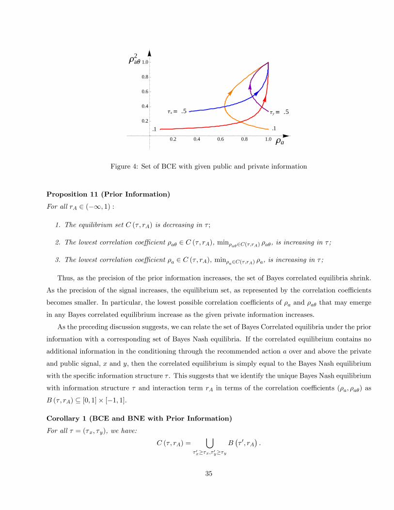
a2

a

x .5

.1

y .5

.1

0.2 0.4 0.6 0.8 1.0

0.2

0.4

0.6

0.8

1.0

Figure 4: Set of BCE with given public and private information

Proposition 11 (Prior Information)

For all rA 2 (�1; 1) :

1. The equilibrium set C (� ; rA) is decreasing in � ;

2. The lowest correlation coe¢ cient �a� 2 C (� ; rA), min�a�2C(�;rA) �a�, is increasing in � ;

3. The lowest correlation coe¢ cient �a 2 C (� ; rA), min�a2C(�;rA) �a, is increasing in � ;

Thus, as the precision of the prior information increases, the set of Bayes correlated equilibria shrink.

As the precision of the signal increases, the equilibrium set, as represented by the correlation coe¢ cients

becomes smaller. In particular, the lowest possible correlation coe¢ cients of �a and �a� that may emerge

in any Bayes correlated equilibrium increase as the given private information increases.

As the preceding discussion suggests, we can relate the set of Bayes Correlated equilibria under the prior

information with a corresponding set of Bayes Nash equilibria. If the correlated equilibrium contains no

additional information in the conditioning through the recommended action a over and above the private

and public signal, x and y, then the correlated equilibrium is simply equal to the Bayes Nash equilibrium

with the speci�c information structure � . This suggests that we identify the unique Bayes Nash equilibrium

with information structure � and interaction term rA in terms of the correlation coe¢ cients (�a; �a�) as

B (� ; rA) � [0; 1]� [�1; 1].

Corollary 1 (BCE and BNE with Prior Information)

For all � = (�x; �y), we have:

C (� ; rA) =[

� 0x��x;� 0y��y

B�� 0; rA

�.

35

In Section 5.5, we extended the analysis of the Bayes correlated equilibrium from an environment with

pure common values to an environment with interdependent values. Similarly, we can extend the analysis

of prior information, pursued here in some detail for the pure common value, to the interdependent value

environment. In particular, we could ask how the equilibrium set with interdependent values is impacted

by prior information about the agent. Given that each agent has a distinct payo¤ state �i, a natural

extension of the private and public signal is given by:

xi = � + �i + "i;

and

yi = � + �i + ";

where the random variables "i and " are normally distributed with zero mean and variance given by �2x

and �2y, respectively; moreover "i and " are independently distributed, with respect to each other and the

state � + �i. The interpretation is now that each agent receives at least some information about the state

�i = � + �i, where the signal xi has an error "i which is idiosyncratic to agent i, and the signal yi has a

error " which is common to all the agents. Thus, the public aspect of the signal yi in the interdependent

world is weaker than in the pure common value case. Each agent i receives a distinct signal yi = �+�i+ ",

due to the private component �i, but the signal yi shares a common shock " across the agents, and hence

might correlate the actions of the agents. Now, the �rst basic result, Proposition 11.1, namely that the

equilibrium set C (� ; rA) is shrinking in the precision of the prior information continues to hold for all

interdependent value environments, including the case of pure private values. Similarly, the second basic

result, Proposition 11.2, namely that the lowest correlation coe¢ cient �a�i in the equilibrium set C (� ; rA),

min�a�i2C(�;rA)�a�i , is increasing in the precision of the prior information remains to hold. Of course, with

interdependent values, the correlation of the individual action a with the individual state �i is composed

of the correlation that arises with the private and public component of the state �i, or

�a�i�a

q�2� + �

2� = �a��a�� + �a��a�� .

The above decomposition of the covariance already hints how the �nal result, Proposition 11.3, generalizes

in the interdependent value environment. With interdependent values, an increase in the precision of prior

information, will not only sharpen the lower bound on the correlation coe¢ cient �a, but also sharpen the

upper bound on �a. In fact, the novel restriction arising in the interdependent value environment are

probably easiest illustrated with the pure private value environment. In the private value environment,

the correlation (coe¢ cient) �a�i of the individual action ai with the individual state �i does not provide

a lower bound for the correlation coe¢ cient �a of the actions across agents, but does provide an upper

36

bound. As the correlation with the private state increases across agents, the correlation of the across the

actions of the agents necessarily has to decrease. We recall that the restrictions for the interdependent

value environment were given by (33):

�a � �2a� � 0; 1� �a � �2a� � 0,

Now, in a pure private value environment, by hypothesis, the correlation with the common component �

equals zero, and hence only the second inequality has to be considered. If the agents are known to have

prior information about their private state �i = �i, then this increases the lower bound on the correlation

�a� . But in contrast to the pure common value model, this now provides a sharper upper bound on the

correlation across actions, �a. In between the pure private and the pure common value, both forces are

present, and hence the lower and upper bound for �a are converging against an intermediate value as the

precision of the prior information increases.

We illustrate the impact of prior information in the case of the pure private value environment in

Figure 5. In the pure private value environment, an increase in the precision of the private signal, acts

just like an increase in the precision of the public signal in the pure common value environment. The

only di¤erence being, that the increase in the precision now provides an improved upper bound on the

correlation coe¢ cient �a, and hence an increase in the precision of the private signal lowers the correlation

across agents. Similarly, an increase in the precision of the public signal, acts just like an increase in the

precision of the private signal in the pure common value environment. The symmetry across environments

is evident, in the private value environment, the public signal while providing information about the private

state supports more correlation in the actions across the agents, as the agents respond to a common shock.

By extension, the nature of the additional information about the private value in any correlated equilibrium

has to be very good to undo the correlation across agents, and hence the level curve of the public signal in

the private value environment is �atter than that of the private signal. By comparison and by symmetry,

it is the level curve is �at just like the private signal level curve in the common value environment.

In the companion paper, Bergemann and Morris (2011), we consider a canonical game theoretic envi-

ronment with �nite actions and �nite states. We establish a general relationship between the set of Bayes

correlated equilibrium and the nature of the prior information. There we o¤er a multi-agent generalization

of Blackwell�s information ordering which allows to present necessary and su¢ cient conditions as to when

better prior information narrows the set of Bayes correlated equilibrium prediction. The result there mir-

ror the present results. The advantage of the present setting, quadratic payo¤s and normally distributed

uncertainty, is that we can give explicit descriptions of the equilibrium sets in terms of the �rst and second

moments, and their responsiveness to the precision of the prior information. By contrast, in Bergemann

and Morris (2011), we simply establish inclusion and contraction properties, but cannot explicit describe

37

a

a

x 1

x .5y 1

y .5

0.2 0.4 0.6 0.8 1.0

0.2

0.4

0.6

0.8

1.0

Figure 5: Set of BCE with given public and private information with pure private values

the equilibrium set in terms of the �rst and second moments anymore.

7 Robust Identi�cation

So far, our analysis has been concerned with the predictive implications of Bayes correlated and Bayes

Nash equilibrium. In particular, we have been asking what are the restrictions imposed by the structural

model on the observed endogenous statistics about the actions of the agents. In this section we pursue

the converse question, namely the issue of identi�cation. We ask what restrictions can be imposed on the

parameters of interest, namely the structural parameters of the game by the observed variables? We are

particularly interested in how the identi�cation of the structural parameters is in�uenced by the solution

concept, and hence the speci�cation of the private information of the agents as known to the analyst.

Now, identi�cation may depend critically on what types of data are available. We therefore consider

�rst the possibility of identi�cation with individual data, and then with aggregate data. The identi�cation

with aggregate data is centered around the canonical problem of demand and supply identi�cation. In

contrast to the received work on identi�cation in the demand and supply model we allow for incomplete

information by the market participants. The problem of identi�cation in the demand and supply model

relies only on aggregate data about the action of the agents, the aggregate quantity and the price, which

constitutes a linear combination of the aggregate action and the realized state of the world.

We should emphasize that the current payo¤ environment describes a common value environment, i.e.

the state of the world is the same for all the agents. In contrast, much of the small, but growing literature on

identi�cation in games with incomplete information is concerned with a private value environment, in which

the private information of agent i only a¤ects the utility of agent i, as for example in Sweeting (2009), Bajari,

38

Hong, Krainer, and Nekipelov (2010) or Paula and Tang (2011). A second important distinction is that in

the above mentioned papers, the identi�cation is about some partial aspect of the utility functions and the

distribution of the (idiosyncratic) states of the world, whereas the present identi�cation seeks to identify

the entire utility function but assumes that the states of the world are observed by the econometrician.

7.1 Robust Identi�cation with Individual Data

We now consider the strategic environment and assume for the remainder of this subsection that the

econometrician observes the individual actions ai and the state �. In other words, the econometrician learns

the �rst and second moment of the joint equilibrium distribution over actions and state: (�a; �a; �a; ��; �a�).

We begin the identi�cation analysis under the hypothesis of Bayes Nash equilibrium and a given information

structure � of the agents. We �nd that the slope of the equilibrium response and the sign of the interaction

parameters are identi�ed for every information structure of the game.

Proposition 12 (Point Identi�cation in BNE)

The Bayes Nash equilibrium with information structure � ,

1. identi�es the sign of the informational externality a�;

2. identi�es the sign of the strategic interaction aA if 0 < �x; �y <1; and

3. identi�es the ratios, a�= ( a + aA) and �a= ( a + aA).

The individual terms of the payo¤ function, namely a; a� and aA cannot be point identi�ed in the

Bayes Nash equilibrium. As the marginal cost parameter a of the private action scales all the relevant

best response and hence equilibrium condition, we cannot expect the point identi�cation of the interaction

parameters a� and aA, even in the complete information environment.

We contrast the point identi�cation for any speci�c information structure with the set identi�cation

in the Bayes correlated equilibrium. We do not make a speci�c hypothesis regarding the information

structure of the agents, and ask what we learn from the data in the absence of speci�c knowledge of the

information structure. Now, from the observation of the covariance �a��a�� and the observation of the

aggregate variance �a�2a, we can identify the values of �a� and �a. The equilibrium conditions which tie

the data to the structural parameters are given by the following conditions on mean and variance:

�a = ��a + �� a� a + aA

; (43)

and

�a = ��� a��a��a aA + a

: (44)

39

We thus have two restrictions to identify the four unknown structural parameters (�a; a; a�; aA). We can

solve for two of the unknowns in terms of the remaining unknowns. In particular, when we solve for (�a; a�)

in terms of the remaining unknowns, a and aA, we obtain expressions for the equilibrium intercept and

the equilibrium slope in terms of the moments and the remaining unknown structural parameters:

� �a a + aA

= �a ��a�� ( a + �a aA)

�� ( a + aA) �a�;

and

� a� a + aA

=�a

�a���

a + �a aA a + aA

: (45)

Now, except for the case of �a = 1, in which the agents are all perfectly correlated, we �nd that the

ratio on the lhs is not uniquely determined. As the strategic interaction parameter aA can vary, or

aA 2 (�1;� a), it follows that we can only partially identify the above ratios, namely,

� �a a + aA

2

8<:��1; �a �

���a�a�a���

�if ��

�a�> 0;�

�a ����a�a�a���

;1�

if ���a�

< 0;

and the above ratio is point-identi�ed if �� = 0. Similarly,

� a� a + aA

2

8<:��a�a�a���

;1�

if �a� > 0;��1; �a�a�a���

�if �a� < 0:

(46)

which describes the respective sets into which each ratio can be identi�ed.

Proposition 13 (Set Identi�cation in BCE)

The Bayes correlated equilibria:

1. identify the sign of the informational externality a�;

2. do not identify the sign of the strategic interaction aA;

3. identify a set of response ratios given by (46) if �a < 1.

Thus, in comparison to the Bayes Nash equilibrium, the Bayes correlated equilibrium, weakens the

possibility of identi�cation in two respects. First, we fail to identify the sign of the strategic interaction

aA; second, we can identify only a set of possible interaction ratios. Given the sharp di¤erences in the

identi�cation under Bayes Nash and Bayes correlated equilibrium, we now try to provide some intuition as

to the source of the contrasting results. For a given information structure � and an observed moments of the

Bayes Nash equilibrium distribution, (�a; �a; �a; ��; �a�), we can identify the weights on the private signal

and the public signal, ��x and ��y, directly from the variance of the (aggregate) action and the covariance of

40

the (aggregate) action with the state, see (15). Now, we can use the property of the equilibrium strategy,

namely that the ratio of the weights is exactly equal the precision of the private and public signal, de�ated

by their (strategic) weight, see (13).��x��y=�x�y

a + aA a

:

Thus given the knowledge of the information structure, we can infer the sign of the strategic interaction

term aA from the ratio of the linear weights, ��x and ��y. attribute how much of the variance in the action

, individual or aggregate, is attributable to the private and the public signal respectively. Given the known

strength of the signals, the covariance of the action and the state then allow us to identify the slope of the

equilibrium response. In the identi�cation under the hypothesis of the Bayes correlated equilibrium, we

observe and use the same data as under the Bayes Nash equilibrium, but now we do not know anymore how

precise or noisy the information of the agents is. Thus, we now face an attribution problem as the observed

covariance between the action and the state could be large either because the individual preferences are

very responsive to the state, i.e. a� is large, or because the agents have very precise information about

the state and hence respond strongly to the precise information, even though they are only moderately

sensitive to the state, i.e. a� is low.

This attribution problem, which is present when the agent�s information structure is not known, is

often referred to as �attenuation bias�in the context of individual decision making. The basic question is

how much we can learn from the observed data when the analyst cannot be certain about the information

that the agent has when he chooses his action. In the single agent context, the noisy signal x that

the agent receives about the state of world � leads to noise in the predictor variable. The noise in the

predictor variable introduces a bias, the �attenuation bias�. Yet in the single agent model, the sign of the

parameter of the interest, the informational externality a� remains correctly identi�ed, even though the

information externality is set-identi�ed rather than point-identi�ed. Importantly, as we extend the analysis

to strategic interaction, the �attenuation bias� critically a¤ects the ability to identify the nature of the

strategic interaction. In particular, the set-identi�ed information externality �covers�the size of strategic

externality to the extent that we may not even identify the sign of the strategic interaction, i.e. whether

the agents are playing a game of strategic substitutes or complements.

Given the lack of identi�cation in the absence of knowledge regarding the information structure, it is

natural to ask whether prior information can improve the identi�cation of the structural parameters, just

as prior information could improve the equilibrium prediction. This is the content of the next propositions.

The econometrician observes the following data (or moments), denoted by m = (�a; ��; �a; �a�; �a; ��)

and is now assumed to know the structure of the prior information � = (�x; �y). We ask how the iden-

ti�cation of the sign of aA and the set identi�cation of the equilibrium slope a� a+ aA

is a¤ected by the

41

knowledge of the prior information � = (�x; �y). We denote the lower and upper bound of the identi�ed

set for the equilibrium slope a� a+ aA

by (� ;m) and (� ;m), respectively. The bounds depend naturally

on the prior information and the observed data. Similarly, we denote the lower and upper bound of the

identi�ed set for the strategic interaction aA by aA (� ;m) and aA (� ;m), respectively.

We observed earlier that the identi�cation of the equilibrium slope in the Bayes correlated equilibrium,

see (45):

� a� a + aA

=�a

�a���

a + �a aA a + aA

;

relied on a ratio of the observed data �a=�a��� and a ratio ( a + �a aA) = ( a + aA) which involves the

unknown structural parameters and the data, where the latter ratio can be rewritten using the earlier

de�ned interaction parameter rA = � aA= a as:

a + �a aA a + aA

=1� �arA1� rA

. (47)

In Section 6, we showed that the knowledge of the information structure � systematically restricts the

equilibrium predictions of the coe¢ cients (�a; �a�). Now, as we consider the identi�cation of the structural

parameters, we use the knowledge of the information structure � together with the data to restrict the

set of structural parameters consistent with the data and the prior information � . In Proposition 11 we

described the set of possible equilibrium coe¢ cients (�a; �a�) as a function of the prior information � and

the interaction parameter rA. Now, that we observe (�a; �a�), we may ask which values of the interaction

parameter rA are consistent with the observed data. To this end we need to know the set of possible

equilibrium correlation coe¢ cients (�a; �a�) varies with the interaction parameter rA of the game.

Proposition 14 (Prior Information and Interaction)

For all � 2 R2+:

1. Cx (� ; rA) is increasing in rA;

2. Cy (� ; rA) is decreasing in rA:

The comparative static results in the interaction parameter rA are straightforward. The information

in the private signal x leads each agent to choose an action which is less correlated with the average action

than the same information contained in the public signal y. Now, as the interaction in the game tends

towards strategic substitutability, each agent tends to rely more heavily on the private signal relative to

the public signal. Thus, for every level of correlation with the state �, expressed in terms of �a�, there will

be less correlation across actions, expressed in terms of �a. The behavior of the equilibrium set Cx (� ; rA)

with respect to the interaction parameter rA is illustrated in Figure 6. Conversely, the restrictions imposed

42

.99

.8

rA ­1

.5x

1 x

a

a

0.2 0.4 0.6 0.8 1.0

0.2

0.4

0.6

0.8

1.0

Figure 6: Bayes correlated equilibrium set with precision �x of prior private information

y

1 y

0 rA 0.5

­1

a

a

­10

­100

0.2 0.4 0.6 0.8 1.0

0.2

0.4

0.6

0.8

1.0

Figure 7: Bayes correlated equilibrium set with precision �y of prior public information

by the public information, represented by the set Cy (�y; rA) become weaker as the game is moving from

strategic complements to strategic substitutes. After all, the public information correlates the agent�s

action because they rely on the same information. If we decrease the propensity to coordinate, and hence

correlate, then all equilibria will display less correlation across actions, for a given correlation with respect

to the state �. The behavior of the equilibrium set Cy (� ; rA) with respect to the interaction parameter

rA is illustrated in Figure 7.We thus �nd that the comparative static results with respect to the strategic

interaction are pointing in the opposite direction for the equilibrium sets Cx (�x; rA) and Cy (�y; rA),

respectively. In consequence, the equilibrium set C (� ; rA) formed by the intersection of the private and

public equilibrium sets, C (� ; rA) = Cx (�x; rA) \ Cy (�y; rA), does not display a monotone behavior in rAin terms of set inclusion.

43

Now, for the set identi�cation of the equilibrium slope given by (47), we have to ask what is the range

of the ratio (1� �arA) = (1� rA) consistent with data. For �a < 1, the value of this ratio is increasing inrA, and hence the greatest possible value of rA, consistent with the data, provides the upper bound for the

above ratio. Now, as a consequence of Proposition 14 the upper bound on rA is given by the restrictions

of the public equilibrium set, and similarly the lower bound is given by the restrictions of the private

information set. To wit, as we increase the interaction parameter rA, the set of correlation coe¢ cients

(�a; �a�) consistent with a given information structure is shrinking in the public equilibrium set, and hence

any given data point (�a; �a�) is eventually eliminated. becomes inconsistent. We therefore improve the

identi�cation with an increase in the precision of the prior information.

Proposition 15 (Equilibrium Slope and Prior Information)

1. The lower bound (� ;m) is increasing in �x and the upper bound (� ;m) is decreasing in �y;

2. The lower bound and the upper bound converge as the prior information becomes precise:

lim�x"1

((�x; �y) ;m) = lim�y"1

@ ((�x; �y) ;m) =�a��a��

.

The above statement shows that the identi�cation improves monotonically with the prior information.

Figure 8 illustrates how prior information improves the set identi�cation. The x�axis represents thepossible values of the slope of the equilibrium response (multiplied by the mean �� of the state �), whereas

the y-axis represents the intercept of the equilibrium response. The observed mean of the equilibrium

action restricts the relationship between the slope and the intercept parameter to a one-dimensional line

with slope �1. The shaded blue lines indicate the possible pair of intercept and slope as a function of theobserved data. As we increase the precision of the public information, the length of the blue line shrinks

(from below), which indicates that the identi�ed set shrinks with an improvement in the lower bound of

the information.

Conversely, if we were to increase the lower bound on the private information, then we would impose

additional restrictions on the linear relationship from above. We can establish a similar improvement with

respect to the sign of the strategic interaction aA, namely the set [ aA (� ;m) ; aA (� ;m)].

Proposition 16 (Interaction Sign and Prior Information)

If �a� < 1 and aA 6= 0, then either there exists �x such that for all 0 < �x < �x:

0 < aA((�x; �y) ;m) < aA ((�x; �y) ;m) ,

or there exists �y such that for all 0 < �y < �y:

aA((�x; �y) ;m) < aA ((�x; �y) ;m) < 0.

44

a a

a

a

a aA

a

a aAa a

a

y

y

y

Figure 8: Set Identi�cation and Prior Public Information: �y > � 0y > � 00y

The identi�cation results here, in particular the contrast between Bayes Nash equilibrium and Bayes

correlated equilibrium, are related to, but distinct from the results presented in Aradillas-Lopez and

Tamer (2008). They compare identi�cation results under di¤erent solution concepts, most notably level

k-rationalizability and Nash equilibrium. In their analysis of an entry game with incomplete information,

they document the loss in identi�cation power that arises with a more permissive solution concept, i.e.

level k-rationalizability. As we compare Bayes Nash and Bayes correlated equilibrium, we show that the

lack of identi�cation is not necessarily due to lack a common prior, as associated with rationalizability, but

rather the richness of possible private information structures (but all with a common prior). Interestingly,

the entry game in Aradillas-Lopez and Tamer (2008) displayed multiple equilibria even under complete

information. In contrast, the class of games we analyze all have a unique equilibrium under either complete

or incomplete information, still a more permissive equilibrium concepts leads to a loss in identi�cation.

An alternative exercise in the current setting would be to limit the identi�cation to a certain subset

of parameters, say the interaction term aA, but then identify the distribution of the states of the world

rather than assuming the observability of the states. For example, Bajari, Hong, Krainer, and Nekipelov

(2010) estimate the peer e¤ect in the recommendation of stocks among stock market analysts in a private

value environment. There, the observables are the recommendations of the stock analysts and analyst

speci�c information about the relationship of the analyst to the recommended �rm. The present analysis

suggest that a similar exercises could be pursued in a common value environment, much like a beauty

contest. A natural extension here would be use of the actual performance of the recommended stocks to

in fact identify the information structure of the stock analysts.

Finally, in many of the recent contributions the assumption of conditional independence of the private

information, relative to the public observables, is maintained. For example, in Paula and Tang (2011), the

45

conditional independence assumption is used to characterize the joint action equilibrium distribution in

terms of the marginal probabilities of every action. Paula and Tang (2011) uses the idea that if private

signals are i.i.d. across individuals, then the players actions must be independent in a single equilibrium,

�but correlated when there are multiple equilibria�to provide a test for multiple equilibria. In contrast, in

our model, we have uniqueness of the Bayes Nash equilibrium, but the unobserved information structure

of the agents could lead to correlation, which would then be interpreted in the above test as evidence

of multiple equilibria, but could simply be due to the unobserved correlation rather than multiplicity of

equilibria.

7.2 Robust Identi�cation with Aggregate Data: Demand and Supply

Next, we consider the possibility of robust identi�cation in the context of demand and supply. We consider

the linear model of demand and supply. We assume that the (inverse) demand function of the representative

consumer is given by:

Pd = �d + adA+ d�d; (48)

and that the inverse supply function of the industry is given by:

Ps = �s + asA+ s�s: (49)

The demand and supply functions (48) and (49) can, as usual, be generated by quadratic utility and cost

functions respectively, see Example 2. The supply of the individual �rm is given by ai and the aggregate

supply is given by A. The canonical analysis of the demand and supply identi�cation uses demand as well

as cost shocks. In the interest of space, here we shall consider only a common supply shock.2 An important

aspect of the demand and supply identi�cation is that it canonically uses only aggregate data, namely the

aggregate quantity, rather than the individual supply data, but then uses a second source of data, namely

the aggregate price, to facilitate the identi�cation. The present identi�cation analysis adheres to this

convention. We can rewrite the demand and supply function in terms of the general notation adopted in

Section 3 by setting:

d , 0; s , a�; as , � a; ad , aA:

In contrast to the classic identi�cation literature, which considers complete information environments,

we are interested in an environment with incomplete information. The state of the world now describes

the supply shock, � = �s, say the level of an input price, and remains normally distributed � � N���; �

2�

�.

2The present analysis can be extended to the canonical model with demand and cost shocks. Here, we do not pursue the

analysis of the associated model with a two-dimensional state � = (�d; �s), as this extension, while entirely straightforward, is

substantially more elaborate as we would have to keep track of the additional interaction and covariance terms.

46

The incomplete information arises as each �rm has to make its supply decision, ai, on the basis of private,

but possibly noisy information, about the common cost shock. The market is cleared by the price which

results from the supplied aggregate quantity A and the level of demand. We determine whether the demand

and supply function can be identi�ed under incomplete information, and more precisely whether it can be

robustly identi�ed, independent of the knowledge of the structure of the private information of the agents.

We begin the analysis with the Bayes Nash equilibrium as a benchmark. We gave a complete analysis

of the Bayes Nash equilibrium in Section 4 and use it for the present identi�cation result. We maintain

the assumption that the information structure, � , but not the signal realizations (xi; y) are known to the

econometrician, and hence can be used to identify the structure of demand and supply. Now, we observed

earlier that the variance of the aggregate action, here the aggregate supply, and the covariance with the

observed cost shock is su¢ cient to identify the linear coe¢ cients of the Bayes Nash equilibrium strategy.

With the separate observation of the equilibrium price P , we can point identify the demand parameter

aA. The variance and covariance then allow us to point identify the supply parameters, a� and a.

Proposition 17 (Point Identi�cation in BNE)

The demand function, aA and the supply function ( a; a�), are point identi�ed for every information

structure 0 < �x; �y <1.

We note that the above identi�cation result uses the positive noise in the private and public signal to

distinguish the demand parameter aA from the supply parameter a. The supply of the individual �rm is

more responsive to the private signal than to the public signal in this game with substitutes. After all, the

private signals are less correlated across agents than the public signal. In an environment with complete

information, where all the agents receive the same noiseless signal about the cost shock, the parameters of

the supply function, a and a�, could not be identi�ed separately. Of course, the slope of the equilibrium

response would still be point-identi�ed.

Next, we consider the possibility of robust identi�cation. As in the Bayes Nash equilibrium, the presence

of the equilibrium price data allows us to point identify the demand parameter aA. The identi�cation of

the supply function is a di¤erent matter. In the presence of the aggregate data, we can only learn from the

aggregate variance �2A and the covariance with the cost shock, �A��A��, which allows us to identify the

correlation coe¢ cient �A�. But in contrast to the Bayes Nash equilibrium, where we could infer from the

aggregate data the behavior of the individual choices, in particular the correlation coe¢ cients �a and �a�,

we now have to contend with additional limitations. The relationship between the individual choices and

the aggregate choices and the aggregate covariance �A� restricts the idiosyncratic correlation coe¢ cients,

47

see (18):

�A� =�a�p�a: (50)

In other words, the data, in particular �A�, allows us to identify a curve in the unit square of the correlation

coe¢ cients (�a; �a�), but not more. In turn, the observation of the mean and variance of the aggregate

supply imposes restriction on the parameters of the supply function, a and a�:

�A = ��a + �� a� a + aA

; (51)

and

�A = ��� a��A��a�a aA + a

= ��� a��a�

p�a

�a aA + a; (52)

yet these two restrictions are not su¢ cient to point identify either a and a�, or even the slope of the

equilibrium supply, a�= ( a + aA). In fact by inspecting (51) and (52), we �nd that we face three unknown

structural parameters (�a; a; a�) and an unknown endogenous parameter, �a.

Proposition 18 (Partial Identi�cation in BCE)

The demand function, aA, is point identi�ed, but the supply function, ( a; a�), is not point identi�ed.

The partial identi�cation is notably asymmetric. The demand structure is completely identi�ed, but

the supply structure is only partially identi�ed. This asymmetry is due entirely to the asymmetry in

which the private information enters the equilibrium variables. We assumed that the �rms make their

supply decision on the basis of their private information about the cost shocks, but that the equilibrium

price, and hence the consumer�s decision was made after the shock had been realized. Thus, the variation

in the equilibrium price, conditional on the supplied quantity, was identi�ed without the interference of

the private information. The identi�cation problem would become more symmetric if instead we were to

assume that the consumer were to make their decision under private information as well, and hence before

the realization of the demand shock. We did not pursue this more elaborate information environment here.

Yet, if we were to pursue it, the basic insight, namely that the private information renders the identi�cation

incomplete would now apply a fortiori, and in particular it would render the demand structure partially

identi�ed as well.

Given the observed variance of the aggregate action, the analyst cannot know whether the variance in

the supply should be attributed to the marginal cost, a or to the sensitivity with respect to cost shock,

a�. In particular, if the supply is very sensitive to the cost shock, then a given variance of the aggregate

quantity, must be explained by a su¢ ciently large marginal cost to dampen the response of the �rm. Using

the above restriction on mean and variance, we know that the equilibrium response is given by:

a� a + aA

= � �A����A

1

�a

a + aA�a a + aA

: (53)

48

The linear condition (53) is similar to the identi�cation issue we faced with individual data in (45). But

there, we could at least infer the correlation coe¢ cient �a from the individual data. By contrast, in the

context of demand and supply, we are restricted to use aggregate observables, and hence do not know �a.

The equilibrium slope is therefore only set-identi�ed, as given the limited data we can only assert that:

a� a + aA

2�x 2 R

����x = � �A���A�

y for some y 2 (1;1)�; (54)

where the second inclusion follows from the fact that we cannot infer the correlation coe¢ cient �a from

the aggregate data.

Now, the interaction between the correlation coe¢ cient �a and the parameter a of the supply function

in (53) suggests that prior information may substantially improve the identi�cation result, just as it is

was shown previously with the individual data. Earlier we noticed that the lower bounds on the private

information imposed lower bounds on the correlation coe¢ cients �a and �a�, see Proposition 11. Now, the

aggregate data only leads to information about the ratio of these two coe¢ cients, but not their size. Thus,

with the lower bounds we narrow the possible range of the individual behavior, and hence the possible

range of the correlation coe¢ cients. At the same time, we saw that the private and public equilibrium sets

respond di¤erently to a change in the parameter of the supply function. In Proposition 14 we showed that

as we increase a, the private equilibrium set shrinks, whereas the public equilibrium set grows.

Now, for a given pair of correlation coe¢ cients (�a; �a�), consistent with (50), we ask how an increase in

the prior information improves the identi�cation. Figure 9 illustrates this with a symmetric increase in the

precision of the public and private signal, or �x = �y. With zero prior information, we see that we cannot

the restrict the value of the interaction ratio. But as we increase the precision of the prior information,

the identi�ed set shrinks rapidly until it is point identi�ed. Now for a given pair of correlation coe¢ cients

in the interior of the unit square, or 0 < �a; �a� < 1, eventually the increase in the precision would require

too large a correlation to be consistent with the observed data, which explains the collapse of the identi�ed

set beyond a speci�c value of the precision � .

Now, with aggregate data, an entire range of correlation coe¢ cients (�a; �a�) is consistent with the

aggregate correlation coe¢ cient �A�. This is illustrated in Figure 10 where we �x the aggregate correlation

coe¢ cient �A� and a particular information structure � and ask what values of the interaction ratio rA

are consistent with a particular �a� and �a. For a given �A�, we plot on the x�axis the possible values of�a� (which then implicitly de�nes the corresponding values of �a). Then given the information structure

� , every vertical segment between the lower boundary de�ned through the public equilibrium set and the

upper boundary de�ned through the private equilibrium set identi�es the set of interaction ratios consistent

with the data. The entire range of interaction ratios consistent with the observed data is therefore given by

the lower bound and the upper bound on the interaction ratio across all �a� with a nonempty. intersection.

49

x y

Private  ES

Public ES

aA

a

1 2 3

1

1

2

3

4

Figure 9: Identi�ed set of strategic interaction ratio aA= a as a function of prior information with precision

�x = �y = �

a

P ublic ES

P rivate ESaA

a

0.80 0.85 0.90 0.95 1.00

1

1

2

3

Figure 10: Identi�ed set of interaction ratio aA= a with aggregate data �A�

While in general the interaction term rA can be positive, given that the demand is point identi�ed with

a negative slope, aA < 0, it follows that the values of the interaction term rA = aA a

have to be positive

everywhere. The shaded area in between the lower and upper boundary, subject to the nonnegativity

condition then presents the identi�ed set.

We denote the lower and upper bound of the identi�ed set for the strategic interaction a by a (� ;m)

and a (� ;m), respectively. The bounds depend naturally on the prior information and the observed data.

Earlier we introduce the lower and upper bounds of the identi�ed set for the equilibrium response a� a+ aA

as (� ;m) and (� ;m), respectively.

50

Proposition 19 (Prior Information and Identi�cation)

1. The lower bound a(� ;m) increases in the precision �y, the upper bound a (� ;m) decreases in the

precision �x.

2. The lower bound (� ;m) increases in the precision �x, the upper bound (� ;m) decreases in the

precision of �y.

3. The lower bounds and the upper bounds converge as the prior information becomes precise:

lim�y"1

a(� ;m) = lim

�x"1@ a (� ;m) = a, lim

�y"1 (� ;m) = lim

�x"1@ (� ;m) =

a� a + aA

.

We analyzed the identi�cation problem in the demand and supply model under the restriction that we

only observed the aggregate supply data rather than the individual supply data. In the case of the Bayes

Nash equilibrium, we showed that the restriction to aggregate data is actually without loss of identi�cation

power. However, in the case of the Bayes Correlated equilibrium, additional information in terms of the

individual supply data would ease the identi�cation problem. The additional information would clearly

help, as the description of the identi�ed set for the equilibrium slope, see (54), indicated. With the

individual supply data, we could infer �a and �a�, rather than just the ratio of the two, which is contained

in the aggregate correlation coe¢ cient �A�, see (50).

8 Conclusion

It was the objective of this paper to derive robust equilibrium predictions for a large class of games. We

began with an epistemic result that related the class of Bayes Nash equilibria with the class of Bayes

correlated equilibria. The equivalence results allowed us to focus on the characterization of the Bayes

correlated equilibria which proceeded without reference to a speci�c information structure held by the

agents. Within a class of quadratic payo¤ environments, we gave a full characterization of the equilibria

in terms of moment restrictions on the equilibrium distributions. The robust analysis allowed us to make

equilibrium predictions independent of the information structure, the nature of the private information

that the agents might have access to.

We then reversed the point of view and considered the problem of identi�cation rather than the problem

of prediction. We asked what are the implication of a robust point of view for identi�cation, namely the

ability to infer the unobservable structural parameters of the game from the observable data. Here we

showed that in the presence of robustness concerns, the ability to identify the underlying parameters of the

game is weakened in important ways, yet does not completely eliminate the possibility of identi�cation. The

51

current perspective, namely to analyze the set of correlated equilibria rather than the Bayes Nash equilibria

under a speci�c information structure, is potentially useful in the emerging econometric analysis of games

of incomplete information. There the identi�cation question is typically pursued for a given information

structure, say independently distributed payo¤ types, and it is of interest to know how sensitive the

identi�cation results are to the structure of the private information. In this context, the robust identi�cation

might be particularly important as we rarely observe data about the nature of the information structure

directly.

We considered a continuum of action spaces, but binary or discrete action games might be of interest

as well. A natural example would be voting games where the unknown state of the world is the quality

of the candidate, and we could then examine what the probability of a quali�ed candidate being elected

is and how it depends on the information structure or the election regime being adopted. We would then

have robust policy implications for the voting rules.

In the present analysis, we use the structure of the quadratic payo¤s, in particular the linear best

response property to derive the �rst and second moments of the correlated equilibrium set. A natural next

step would be to bring the present analysis to Bayesian games with nonlinear strategies. For example, it

would be of considerable interest to ask how the allocations and the revenues in the �rst price auction

di¤er across belief environments.

We would also like to use the equilibrium predictions to o¤er robust versions of policy and welfare

analysis. In many incomplete information environments, a second best or otherwise welfare improving

policy typically relies on and is sensitive to the speci�cation of the belief environment. With the current

analysis, we might be able to recommend robust taxation or information disclosure policies which are

welfare improving across a wide range of belief environments. In particular, we might ask how the nature

of the policy depends on the prior information of the policy maker about the belief environment of the

agents.

52

9 Appendix

Proof of Proposition 2. The characterization of the linear Bayes Nash equilibrium strategy in the

same environment of quadratic payo¤s is given in Proposition 1 of Angeletos and Pavan (2007), the only

di¤erence being a di¤erent labeling of the linear return and interaction parameters, � and �.

Proof of Proposition 6. The variance �2a is given by (27), and inserting �a = �2a� we obtain:

� �� a��a��2a� aA + a

which is maximized at:

j�a�j =r

a aA

,

or �a = a= aA.

Proof of Proposition 7. (1.) The volatility �2A, which is given by:

�a�2a = �a

�� �� a��a��a aA + a

�2;

is increasing in the correlation coe¢ cients �a and j�a�j. The partial derivatives with respect to �a and j�a�jare:

�2��2a�

2a�

( a + �a aA)3 ( a � �a aA) > 0,

and2�a j�a�j�2� 2a�( a + �a aA)

2 > 0,

respectively.

(2.) The dispersion, using (30), is given by:

(1� �a)�2a = (1� �a)�� ���a� a��a aA + a

�2,

and it follows that the dispersion is increasing in j�a�j. The dispersion is monotone decreasing in �a if it isgame of strategic substitutes, and not necessarily monotone if it is a game of strategic complements. The

partial derivative with respect to �a is given by

��2��2a�

2a� ( a + aA + (1� �a) aA)

( a + �a aA)3 .

However by Proposition 5, it follows that �2a� � �a, and we therefore obtain the maximal dispersion at

�2a� = �a. Consequently, we have

(1� �a)�2a = (1� �a) �a�� �� a��a aA + a

�2,

53

and the dispersion reaches an interior maximum at

�a = a

2 a + aA2 (0; 1) ,

irrespective of the nature of the game.

Proof of Proposition 8. Every Bayes Nash equilibrium with an information structure � is clearly

a Bayes correlated equilibrium. It remains to establish that every Bayes correlated equilibrium can be

replicated by a Bayes Nash equilibrium for some information structure � . By Proposition 5, the set of

Bayes correlated equilibria is completely characterized by the pair of correlation coe¢ cients (�a; �a�) with

0 � �a � �2a� � 1;

and

0 � �a � 1.

The correlation coe¢ cients �a and �a� of the Bayes Nash equilibrium can be expressed in terms of the

equilibrium coe¢ cients �x and �y and variances �2�; �2x and �

2y as:

�a� = ��� (�x + �y)q

�2x�2x + �

2y�2y + �

2� (�x + �y)

2; (55)

and

�a =�2y�

2y + �

2� (�x + �y)

2

�2x�2x + �

2y�2y + �

2� (�x + �y)

2 . (56)

It now follows immediately from (55) - (56), and the formulae of ��x and ��y, namely (11) - (12) that we

can recover the corresponding information structure � of the Bayes Nash equilibrium as

�x =

� a + �a aA � �2a� ( a + aA)

���p

1� �a�a� a;

and

�y =

� a + �a aA � �2a� ( a + aA)

���q

�a � �2a��a� ( a + aA);

which completes the proof.

Proof of Proposition 11. We form the conditional expectation using (34) and the equilibrium

conditions for the Bayes correlated equilibrium are then given by (36) and the solution to theses equations

is given by (37)-(39).

(1.) The equilibrium set is described as the set which satis�es the inequalities (41) and (42), where

the correlation coe¢ cients �2ax and �2ay appear separately. By determination of (38) and (39), the square

54

of the correlation coe¢ cient is strictly decreasing in �x and �y, which directly implies that the respective

inequalities become less restrictive, and hence the equilibrium set increases as either �x or �y increase.

(3.) The lowest value of the correlation coe¢ cient �a is achieved when the inequality (41) is met as an

equality. It follows that the minimum is reached at the exterior of the equilibrium set. The equilibrium

set is increasing in � by the previous argument in (1), and hence the resulting strict inequality.

(2.) The lowest value of the correlation coe¢ cient �a� is achieved when the inequalities (41) and (42)

are met as equalities. It follows that the minimum is reached at the exterior of the equilibrium set. The

equilibrium set is increasing in � by the previous argument in (1), and hence the resulting strict inequality.

Proof of Proposition 12. (1.) Given the knowledge of �2�; �2x and �

2y and the information about the

covariates, we can recover the value of the linear coe¢ cients �2x and �2y from variance-covariance matrix

(14), say:

�2x =�2a � �2A�2x

; �2y =�2A�1� �2A�

��2y

: (57)

The value of covariate �A��A��, given by �2� (�x + �y) directly identi�es the sign of the externality a�,

given the composition of the equilibrium coe¢ cients ��x and ��y of the Bayes Nash equilibrium, see (11)

and (12).

(2.) We have from the description of the Bayes Nash equilibrium in Proposition 2 that in every Bayes-

Nash equilibrium, ��x and ��y satisfy the linear relationship:

��y = ��x�2x�2y

a a + aA

:

Now, if 0 < �2x; �2y <1, then we can identify the sign of aA.

(3.) Given the identi�cation of ��x and ��y, we can identify the ratios �an ( a + aA) and a�n ( a + aA).

We recover the mean action �a and the coe¢ cients of the linear strategy, i.e. ��x and �

�y, from the equilib-

rium data. We therefore have three equalities, but four unknown structural parameters (�a; a; aA; a�).

From the equilibrium conditions, namely (10) - (12), we have the values of �a; �x and �y. This allows us

to solve for �a; aA and a� as a function of �a; �x; �y:

�a =1

�y�2�2y

��2x�

2 a�2x�� � �x�a�2 a�2x � �x�y�2 a�2y�� + �x�y a�2x�2y��

� aA =

1

�y�2y

��x a�

2x � �y a�2y

�(58)

a� = � 1

�y�2�2y

��2x�

2 a�2x � �x�y�2 a�2y + �x�y a�2x�2y

�;

55

where all the expressions depend on a, and hence are not identi�ed, as a is not identi�ed. But if we

form the ratios �an ( a + aA) and a�n ( a + aA) with the expressions on the rhs of (58), then we obtainexpressions which do only depend on the observable data, and are hence point identi�ed, and in particular

�a a + aA

=

���2�a�2x + �2�x�2x�� � �2�y�2y�� + �2x�y�2y��

��2�2x

; (59)

and a�

a + aA= �

�x�2�2x � �y�2�2y + �y�2x�2y

�2�2x: (60)

which completes the proof of identi�cation. We observe that, using (57), we could express the ratios (59)

and (60) entirely in terms of the �rst two moments of observed data.

Proof of Proposition 13. (1.) From the observation of the covariance �a��a�� we can infer the sign

and the size of �a�, see (44). Given the information about lhs of (44) and the information of �a�, we can

infer the sign of a�.

(2.) Even though the sign of a� can be established, we cannot extract the unknown variables on the

lhs of (43) in the presence of the linear return term �a, and hence it follows that we cannot sign aA.

(3.) From the observation of the covariance �a��a�� and the observation of the aggregate variance �a�2a,

we can infer the value of �a� and �a. The equilibrium conditions then impose the conditions (43) and (44)

on mean and variance. We thus have two equations to identify the four unknown structural parameters

(�a; a; a�; aA). We can solve for (�a; a�) in terms of the remaining unknowns a and aA to obtain:

�a =�a a�� + �a�a�� aA � �a�� aA�a� � a�a���a�

���a�;

and

a� = ��a a + �a�a aA

���a�:

In particular, we would like to know whether this allows us to identify the ratios:

� �a a + aA

= �a ��a�� ( a + �a aA)

�� ( a + aA) �a�;

or

� a� a + aA

=

1��

�a a+�a�a aA�a�

a + aA=

�a�a���

a + �a aA a + aA

;

in terms of the observables. But, except for the case of �a = 1, we see that this is not the case. As

aA 2 (�1;� a), it follows that we can only partially identify the above ratios, namely,

� �a a + aA

2��1; �a �

�a�a�a���

�;

56

and

� a� a + aA

2��a�a�a���

;1�;

which describes the respective set into which each ratio can be identi�ed.

Proof of Proposition 14. The comparative static results follow directly from the description of the

correlation coe¢ cients �ax and �ay given by (38) and (39). These correlation coe¢ cients are a function of

a and aA. We insert their solution into the inequalities (41) and (42) and solve for the relation between

�a and �a� as we restrict the the inequalities (41) and (42) to be equalities.

Proof of Proposition 15. We know from Proposition 13 that the interaction ratio is a function of

the observed data and the unobserved interaction parameters:

� a� a + aA

=�a

�a���

a + �a aA a + aA

.

The prior information on the private and public information restricts the possible values of a and aA,

and hence the values that the above interaction ratio can attain.

We begin the argument with the public equilibrium set which will provide an upper bound on the ratio

a + �a aA a + aA

. (61)

The above ratio appears in the correlation coe¢ cient �ay as described in (39). The value of the ratio is

maximized when the inequality constraint (42) of the public equilibrium set holds as an equality, and thus

a + �a aA a + aA

= �2a� +�y��j�a�j

q�a � �2a�, (62)

and hence

(� ;m) =�a

�a���

��2a� +

�y��j�a�j

q�a � �2a�

�:

It follows that if the variance �y decreases, then the largest value of the above ratio decreases and as �2y

decreases to zero: a + �a aA a + aA

= �2a�,

which implies that

lim�y#0

(� ;m) =�a j�a�j��

:

Now, consider the private equilibrium set. The ratio (61) does not appear directly in the correlation

coe¢ cient �ax, rather the structural parameters a and aA appear in the form of a ratio. We therefore ask

what feasible pair in the private equilibrium set minimizes the ratio (61). The minimal ratio is achieved

57

by a pair ( a; aA) which solves the inequality (41) as an equality. We can therefore solve for aA in terms

of a. The resulting function aA ( a) is linear in a:

aA = a�x�a�

p1� �a �

�1� �2a�

����

�a � �2a����

:

Hence the minimal value of the ratio (61) does not depend on either a nor aA, and is given by:

a + �a aA a + aA

=

a + �a

� a

�x�a�p1��a�(1��2a�)��(�a��2a�)��

� a +

� a

�x�a�p1��a�(1��2a�)��(�a��2a�)��

� =

��a � �2a�

��� + �a

��x j�a�j

p1� �a �

�1� �2a�

�����

�a � �2a���� +

��x j�a�j

p1� �a �

�1� �2a�

���� ;

(63)

and hence

(� ;m) =�a

j�a�j��

��a � �2a�

��� + �a

��x�a�

p1� �a �

�1� �2a�

�����

�a � �2a���� +

��x�a�

p1� �a �

�1� �2a�

���� .

It is immediate to verify that (� ;m) � (� ;m) for all � and m. It follows from the determination of

(� ;m) that as a function of �x, (� ;m) is decreasing in the standard deviation �x, or in other words, it

is increasing in the precision of the private signal. Moreover as �2x decreases to zero:

a + �a aA a + aA

= �2a�,

and hence

lim�x#0

(� ;m) =�a j�a�j��

;

which concludes the proof.

Proof of Proposition 16. For any given �a, with 0 � �a < 1, the ratio

a + �a aA a + aA

is larger than 1 if and only aA > 0. Thus we can identify the sign of aA if we can establish that the ratio

on the rhs of (63), which determined the lower bound on the equilibrium slope, is larger than 1. Now,

clearly if �a < 1, and if for some �x :

�x��p1� �a �

�1� �2�

��� < 0,

we have ��a � �2�

��� + �a

��x��

p1� �a �

�1� �2�

�����

�a � �2���� +

��x��

p1� �a �

�1� �2�

���� > 1,

then the above ratio will remain above 1 for all �x < �x.

58

Similarly, if for given data the expression on the rhs of (62) is smaller than 1 for some �y :

�2a� +�y���a�

q�a � �2a� < 1,

then it will remain smaller than 1 for all 0 � �y < �y.

Proof of Proposition 17. The parameter of the demand function, aA, is identi�ed as we observe

the aggregate quantity and the aggregate price. The covariance between P and A then identi�es aA. By

Proposition 2, if we know the information structure (�x; �y), we can infer from the equilibrium variance �2A

and covariance �A��A�� of the aggregate action A, the value of the linear coe¢ cients ��x and �

�y. Given

the equilibrium relationship between ��x and ��y as documented by (13), this allows to identify the value of

a given the known value of aA. But, now the composition of the equilibrium coe¢ cient ��x and ��y allow

to point identify a� as well.

Proof of Proposition 18. From the observation of the demand, we get aA point identi�ed, but

then still have to identify a and a�. We observe the covariance �A��A�� and the aggregate variance �2A.

This allows us to identify the correlation coe¢ cient �A�:

�A = ��a + �� a� a + aA

;

and

�A = ��� a��A�

p�a

�a aA + a:

We thus have two equations to identify the four unknown structural parameters (�a; a; a�; �a). We can

solve for (�a; a�) in terms of the remaining unknowns a and �a to obtain:

�a =�A a�� + �A aA�a�� � aA�A

p�a���A� � �A a

p�a���A�p

�a����;

and

a� = ��A a + �A aA�ap

�a���A�:

In particular, we would like to know whether this allows us to identify the ratio:

a� a + aA

= � �A����A

1p�a

a + aA�a a + aA

; (64)

and even the value of a� :

a� = ��A

����A

a + aA�ap�a

: (65)

We see from (64) and (65) that this is impossible (without bounds on the information.)

59

Proof of Proposition 19. It remains to set identify the value of a and a�. From the aggregate

data we can infer �A�, but not �a or �a�. The aggregate covariance �A� is related to �a and �a� through

�A� =�a�p�a: (66)

Thus given �A�, there is a curve, given by (66) in the unit square of (�a; �a�) which is compatible with the

given data m, and in particular �A�. Now consider a prior information structure (�x; �y). We then ask

which pairs (�a; �a�) are compatible with the given information structure. To this end, we need to know

whether for a given pair (�a; �a�) there exists a for the identi�ed value of aA such that the pair (�a; �a�)

is in the intersection of the equilibrium set Cx (� ; rA) \ Cy (� ; rA).By Proposition 14, the public equilibrium set Cy (� ; rA) increases in a and the private equilibrium

set Cx (� ; rA) decreases with a. It follows that for every (�a; �a�) there is a lower bound and an upper

bound, a(� ;m) and a (� ;m), respectively, for which if a satis�es a (� ;m) � a � a (� ;m), then

Cx (� ; rA) \ Cy (� ; rA) \ (�a; �a�) 6= ?. From Proposition 11, we know that an increase in the precision

of the prior information (�x; �y) lead Cx (� ; rA) and Cy (� ; rA) to shrink. Eventually as (�x; �y) increase

su¢ ciently, a(� ;m) = a (� ;m). At this point, we have point-identi�ed a at a singleton (�a; �a�), and

hence it follows from (65) that we also have point identi�ed a�. Since the interval ish a(� ;m) ; a (� ;m)

iis shrinking with a decrease in the variance, it follows from the monotonicity of the rhs of (64) that the

identi�ed set is also shrinking with a increase in the precision of the public and private information.

60

References

Angeletos, G., and A. Pavan (2007): �E¢ cient Use of Information and Social Value of Information,�

Econometrica, 75, 1103�1142.

(2009): �Policy with Dispersed Information,�Journal of the European Economic Association, 7,

11�60.

Aradillas-Lopez, A., and E. Tamer (2008): �The Identi�cation Power of Equilibrium in Simple

Games,�Journal of Business and Economic Statistics, 26, 261�283.

Aumann, R. (1987): �Correlated Equilibrium as an Expression of Bayesian Rationality,�Econometrica,

55, 1�18.

Bajari, P., H. Hong, J. Krainer, and D. Nekipelov (2010): �Estimating Static Models of Strategic

Interaction,�Journal of Business and Economic Statistics, 28, 469�482.

Bergemann, D., and S. Morris (2005): �Robust Mechanism Design,�Econometrica, 73, 1771�1813.

(2011): �Correlated Equilibrium in Games of Incomplete Information,�Discussion paper, Cowles

Foundation for Research in Economics, Yale University and Princeton University.

Bergemann, D., S. Morris, and S. Takahashi (2010): �Interdependent Preferences and Strategic Dis-

tinguishability,�Discussion Paper 1772, Cowles Foundation for Research in Economics, Yale University.

Bergemann, D., and M. Pesendorfer (2007): �Information Structures in Optimal Auctions,�Journal

of Economic Theory, 137, 580�609.

Bergemann, D., and J. Välimäki (2002): �Information Acquisition and E¢ cient Mechanism Design,�

Econometrica, 70, 1007�1033.

Blackwell, D. (1953): �Equivalent Comparison of Experiments,�Annals of Mathematics and Statistics,

24, 265�272.

Brillinger, D. (1969): �The Calculation of Cumulants Via Conditioning,� Annals of the Institute of

Statistical Mathematics, 21, 215�218.

Chwe, M. (2006): �Incentive Compatibility Implies Signed Covariance,�Discussion paper, UCLA.

Clarke, R. (1983): �Collusion and the Incentives for Information Sharing,�Bell Journal of Economics,

14, 383�394.

61

Dasgupta, P., and E. Maskin (2000): �E¢ cient Auctions,� Quarterly Journal of Economics, 115,

341�388.

Forges, F. (1993): �Five Legitimate De�nitions of Correlated Equilibrium in Games with Incomplete

Information,�Theory and Decision, 35, 277�310.

Guesnerie, R. (1992): �An Exploration of the Eductive Justi�cations of the Rational-Expectations Hy-

pothesis,�American Economic Review, 82, 1254�1278.

Jehiel, P., and B. Moldovanu (2001): �E¢ cient Design with Interdependent Valuations,�Economet-

rica, 69, 1237�1259.

Jehiel, P., B. Moldovanu, M. Meyer-Ter-Vehn, and B. Zame (2006): �The Limits of Ex Post

Implementation,�Econometrica, 74, 585�610.

Kajii, A., and S. Morris (1997): �The Robustness of Equilibria to Incomplete Information,�Economet-

rica, 65, 1283�1309.

Kamenica, E., and M. Gentzkow (2010): �Bayesian Persuasion,� American Economic Review, p.

forthcoming.

Lehrer, E., D. Rosenberg, and E. Shmaya (2010): �Signaling and Mediation in Games with Common

Interest,�Games and Economic Behavior, 68, 670�682.

(2011): �Garbling of Signals and Outcome Equivalence,�Discussion paper, Tel Aviv University,

University of Paris and Northwestern University.

Morris, S., and H. Shin (2002): �Social Value of Public Information,�American Economic Review, 92,

1521�1534.

Neyman, A. (1997): �Correlated Equilibrium and Potential Games,� International Journal of Game

Theory, 26, 223�227.

Novshek, W., and H. Sonnenschein (1982): �Ful�lled Expectations Cournot Duopoly with Information

Acquisition and Release,�Bell Journal of Economics, 13, 214�218.

Paula, A. D., and X. Tang (2011): �Inference of Signs of Interaction E¤ects in Simultaneous Games

with Incomplete Information,�Econometrica, forthcoming.

Raith, M. (1996): �A General Model of Information Sharing in Oligopoly,�Journal of Economic Theory,

71, 260�288.

62

Sweeting, A. (2009): �The Strategic Timing of Radio Commercials: An Empirical Analysis Using Mul-

tiple Equilibria,�RAND Journal of Economics, 40, 710�742.

Vives, X. (1984): �Duopoly Information Equilibrium: Cournot and Bertrand,� Journal of Economic

Theory, 34, 71�94.

(1990): �Nash Equilibrium with Strategic Complementarities,� Journal of Mathematical Eco-

nomics, 19, 305�321.

63