robotic motion planning: potential functions
TRANSCRIPT

16-735, Howie Choset, with slides from Ji Yeong Lee, G.D. Hager and Z. Dodds
Robotic Motion Planning:Potential Functions
Robotics Institute 16-735http://voronoi.sbp.ri.cmu.edu/~motion
Howie Chosethttp://voronoi.sbp.ri.cmu.edu/~choset

16-735, Howie Choset, with slides from Ji Yeong Lee, G.D. Hager and Z. Dodds
The Basic Idea
• A really simple idea:
– Suppose the goal is a point g∈ ℜ2
– Suppose the robot is a point r ∈ ℜ2
– Think of a “spring” drawing the robot toward the goal and away from obstacles:
– Can also think of like and opposite charges

16-735, Howie Choset, with slides from Ji Yeong Lee, G.D. Hager and Z. Dodds
Another Idea
• Think of the goal as the bottom of a bowl
• The robot is at the rim of the bowl
• What will happen?

16-735, Howie Choset, with slides from Ji Yeong Lee, G.D. Hager and Z. Dodds
The General Idea
• Both the bowl and the spring analogies are ways of storing potential energy
• The robot moves to a lower energy configuration
• A potential function is a function U : ℜm → ℜ
• Energy is minimized by following the negative gradient of the potential energy function:
• We can now think of a vector field over the space of all q’s ...– at every point in time, the robot looks at the vector at the point and goes in
that direction

16-735, Howie Choset, with slides from Ji Yeong Lee, G.D. Hager and Z. Dodds
Attractive/Repulsive Potential Field
– Uatt is the “attractive” potential --- move to the goal
– Urep is the “repulsive” potential --- avoid obstacles

16-735, Howie Choset, with slides from Ji Yeong Lee, G.D. Hager and Z. Dodds
Artificial Potential Field Methods:Attractive Potential
)(
)()(
goal
attatt
qk
qUqF
δ−=
−∇=
Conical Potential
Quadratic Potential

16-735, Howie Choset, with slides from Ji Yeong Lee, G.D. Hager and Z. Dodds
Artificial Potential Field Methods:Attractive Potential
Combined Potential
In some cases, it may be desirable to have distance functions that grow more slowly to avoid huge velocities far from the goal
one idea is to use the quadratic potential near the goal (< d*) and the conic farther awayOne minor issue: what?
16-735, Howie Choset, with slides from Ji Yeong Lee, G.D. Hager and Z. Dodds
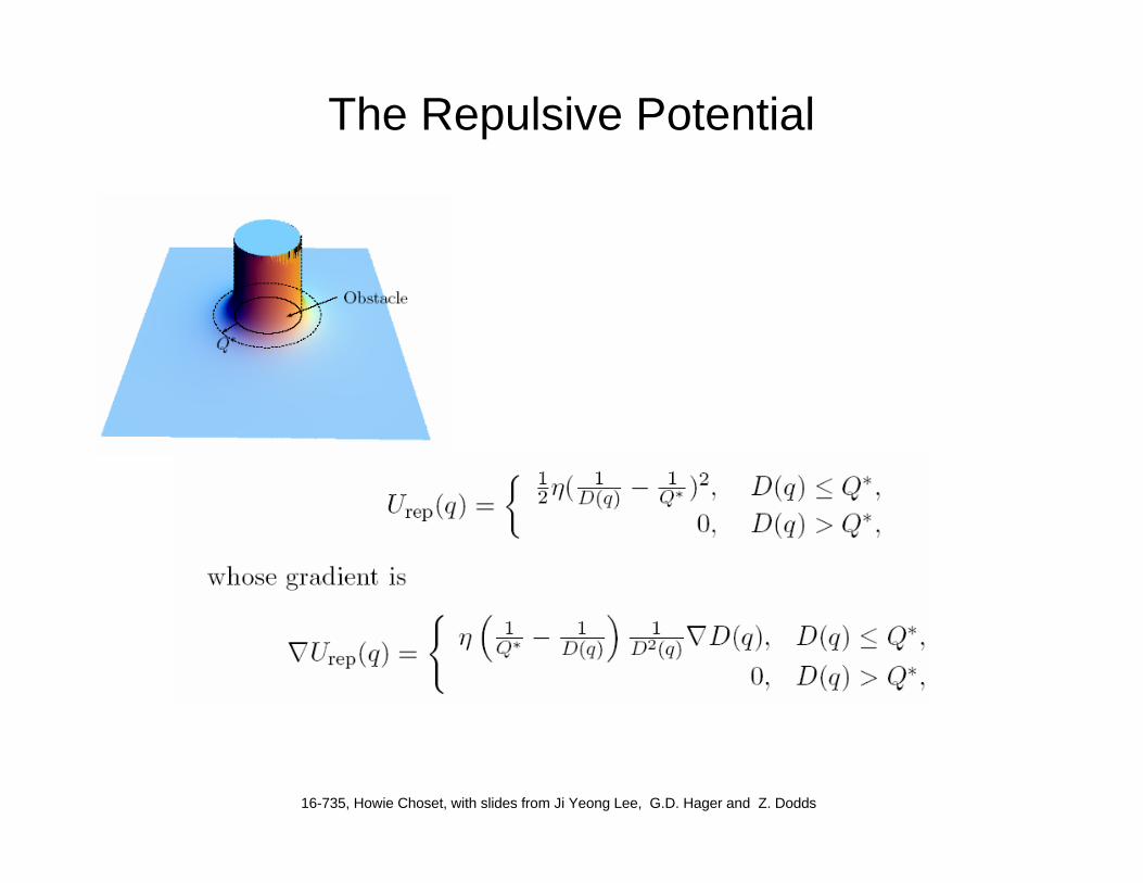
The Repulsive Potential

16-735, Howie Choset, with slides from Ji Yeong Lee, G.D. Hager and Z. Dodds
Repulsive Potential
16-735, Howie Choset, with slides from Ji Yeong Lee, G.D. Hager and Z. Dodds
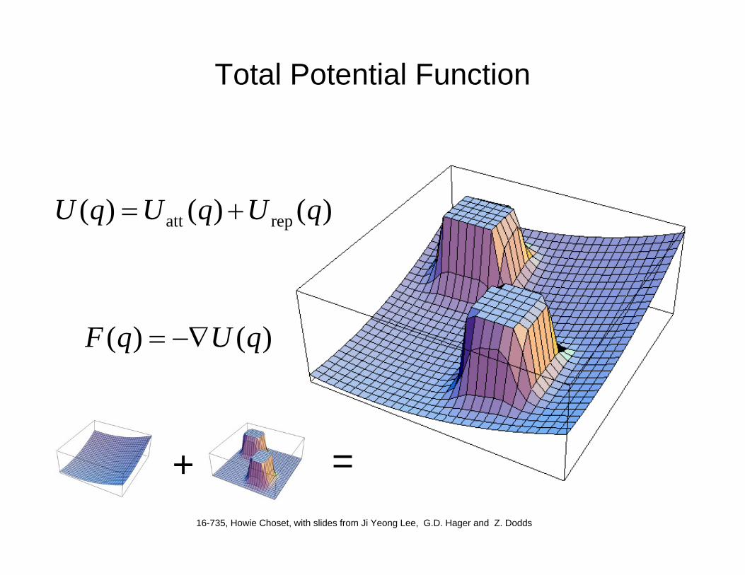
Total Potential Function
+ =
)()()( repatt qUqUqU +=
)()( qUqF −∇=

16-735, Howie Choset, with slides from Ji Yeong Lee, G.D. Hager and Z. Dodds
Potential Fields
16-735, Howie Choset, with slides from Ji Yeong Lee, G.D. Hager and Z. Dodds
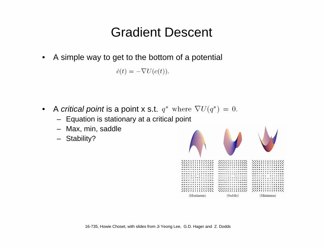
Gradient Descent
• A simple way to get to the bottom of a potential
• A critical point is a point x s.t. ∇U(x) = 0– Equation is stationary at a critical point– Max, min, saddle– Stability?

16-735, Howie Choset, with slides from Ji Yeong Lee, G.D. Hager and Z. Dodds
The Hessian
• For a 1-d function, how do we know we are at a unique minimum (or maximum)?
• The Hessian is the m× m matrix of second derivatives
• If the Hessian is nonsingular (Det(H) ≠ 0), the critical point is a unique point– if H is positive definite (x^t H x > 0), a minimum– if H is negative definite, a maximum– if H is indefinite, a saddle point

16-735, Howie Choset, with slides from Ji Yeong Lee, G.D. Hager and Z. Dodds
Gradient Descent
Gradient Descent:– q(0)=qstart– i = 0– while ∇ U(q(i)) ≠ 0 do
• q(i+1) = q(i) - α(i) ∇ U(q(i))• i=i+1
16-735, Howie Choset, with slides from Ji Yeong Lee, G.D. Hager and Z. Dodds
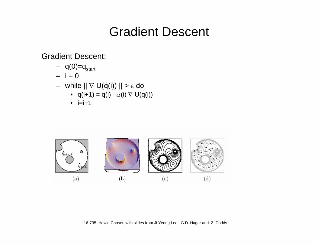
Gradient Descent
Gradient Descent:– q(0)=qstart– i = 0– while || ∇ U(q(i)) || > ε do
• q(i+1) = q(i) - α(i) ∇ U(q(i))• i=i+1

16-735, Howie Choset, with slides from Ji Yeong Lee, G.D. Hager and Z. Dodds
Numerically “Smoother” Path

16-735, Howie Choset, with slides from Ji Yeong Lee, G.D. Hager and Z. Dodds
Single Object Distance

16-735, Howie Choset, with slides from Ji Yeong Lee, G.D. Hager and Z. Dodds
Compute Distance: Sensor Information

16-735, Howie Choset, with slides from Ji Yeong Lee, G.D. Hager and Z. Dodds
Computing Distance: Use a Grid
• use a discrete version of space and work from there
– The Brushfire algorithm is one way to do this• need to define a grid on space • need to define connectivity (4/8)• obstacles start with a 1 in grid; free space is zero
4 8

16-735, Howie Choset, with slides from Ji Yeong Lee, G.D. Hager and Z. Dodds
Brushfire Algorithm
• Initially: create a queue L of pixels on the boundary of all obstacles
• While L ≠ ∅– pop the top element t of L– if d(t) = 0,
• set d(t) to 1+mint’ ∈ N(t),d(t) ≠ 0 d(t’)• Add all t’∈ N(t) with d(t)=0 to L (at the end)
• The result is a distance map d where each cell holds the minimum distance to an obstacle.
• The gradient of distance is easily found by taking differences with all neighboring cells.

16-735, Howie Choset, with slides from Ji Yeong Lee, G.D. Hager and Z. Dodds
Brushfire example

16-735, Howie Choset, with slides from Ji Yeong Lee, G.D. Hager and Z. Dodds
Potential Functions Question
• How do we know that we have only a single (global) minimum
• We have two choices:– not guaranteed to be a global minimum: do something other than gradient
descent (what?)
– make sure only one global minimum (a navigation function, which we’ll see later).

16-735, Howie Choset, with slides from Ji Yeong Lee, G.D. Hager and Z. Dodds
The Wave-front Planner
• Apply the brushfire algorithm starting from the goal
• Label the goal pixel 2 and add all zero neighbors to L– While L ≠ ∅
• pop the top element of L, t• set d(t) to 1+mint’ ∈ N(t),d(t) > 1 d(t’)• Add all t’∈ N(t) with d(t)=0 to L (at the end)
• The result is now a distance for every cell– gradient descent is again a matter of moving to the neighbor with the
lowest distance value

16-735, Howie Choset, with slides from Ji Yeong Lee, G.D. Hager and Z. Dodds
The Wavefront Planner: Setup

16-735, Howie Choset, with slides from Ji Yeong Lee, G.D. Hager and Z. Dodds
The Wavefront in Action (Part 1)
• Starting with the goal, set all adjacent cells with “0” to the current cell + 1– 4-Point Connectivity or 8-Point Connectivity?– Your Choice. We’ll use 8-Point Connectivity in our example
16-735, Howie Choset, with slides from Ji Yeong Lee, G.D. Hager and Z. Dodds
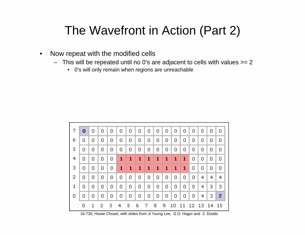
The Wavefront in Action (Part 2)
• Now repeat with the modified cells– This will be repeated until no 0’s are adjacent to cells with values >= 2
• 0’s will only remain when regions are unreachable

16-735, Howie Choset, with slides from Ji Yeong Lee, G.D. Hager and Z. Dodds
The Wavefront in Action (Part 3)
• Repeat again...

16-735, Howie Choset, with slides from Ji Yeong Lee, G.D. Hager and Z. Dodds
The Wavefront in Action (Part 4)
• And again...

16-735, Howie Choset, with slides from Ji Yeong Lee, G.D. Hager and Z. Dodds
The Wavefront in Action (Part 5)
• And again until...
16-735, Howie Choset, with slides from Ji Yeong Lee, G.D. Hager and Z. Dodds
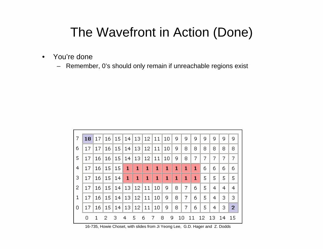
The Wavefront in Action (Done)
• You’re done– Remember, 0’s should only remain if unreachable regions exist

16-735, Howie Choset, with slides from Ji Yeong Lee, G.D. Hager and Z. Dodds
The Wavefront, Now What?
• To find the shortest path, according to your metric, simply always move toward a cell with a lower number
– The numbers generated by the Wavefront planner are roughly proportional to their distance from the goal
Twopossibleshortestpathsshown

16-735, Howie Choset, with slides from Ji Yeong Lee, G.D. Hager and Z. Dodds
Another Example

16-735, Howie Choset, with slides from Ji Yeong Lee, G.D. Hager and Z. Dodds
Wavefront (Overview)
• Divide the space into a grid.• Number the squares starting at the start in either 4 or 8 point
connectivity starting at the goal, increasing till you reach the start.• Your path is defined by any uninterrupted sequence of
decreasing numbers that lead to the goal.
16-735, Howie Choset, with slides from Ji Yeong Lee, G.D. Hager and Z. Dodds
Navigation Functions
• A function φ: Qfree → [0,1] is called a navigation function if it– is smooth (or at least C2)– has a unique minimum at qgoal
– is uniformly maximal on the boundary of free space– is Morse
• A function is Morse if every critical point (a point where the gradient is zero) is isolated.
• The question: when can we construct such a function?

16-735, Howie Choset, with slides from Ji Yeong Lee, G.D. Hager and Z. Dodds
Sphere World
• Suppose that the world is a sphere of radius r0 centered at q0containing n obstacles of radius ri centered at qi, i=1 .. n– β0(q) = -d2(q,q0) + r0
2
– βi(q) = d2(q,qi) - ri2
• Define β(q) = ∏ βi(q) (Repulsive)– note this is zero on any obstacle boundary, positive in free space and
negative inside an obstacle
• Define (Attractive)– note this will be zero at the goal, and increasing as we move away– κ controls the rate of growth

16-735, Howie Choset, with slides from Ji Yeong Lee, G.D. Hager and Z. Dodds
Sphere World
• Consider now – O(q) is only zero at the goal– O(q) goes to infinity at the boundary of any obstacle– By increasing κ, we can make the gradient at any direction point
toward the goal– It is possible to show that the only stationary point is the goal, with
positive definite Hessian because• therefore no local minima
• In short, following the gradient of O(q) is guaranteed to get to the goal (for a large enough value of κ)

16-735, Howie Choset, with slides from Ji Yeong Lee, G.D. Hager and Z. Dodds
An Example: Sphere World• One problem: the value of O(q) may be very large
• A solution: introduce a “switch” σλ(x) = x/(λ + x)
• Now, define O’λ(q) = σλ(O(q))– this bounds the value of the function– however, O’ may turn out not to be Morse
• A solution: introduce a “sharpening function” ηκ(x) = x1/κ
For large enough κ, this is a navigation function on the sphere world!
0,)( >+
= λλ
σ λ xxx

16-735, Howie Choset, with slides from Ji Yeong Lee, G.D. Hager and Z. Dodds
Navigation Function for Sphere World
• For sufficiently large k, k(q) is a navigation
function
-4 -2 0 2 4
-4
-2
0
2
4
-4 -2 0 2 4
-4
-2
0
2
4
-4 -2 0 2 4
-4
-2
0
2
4
-4 -2 0 2 4
-4
-2
0
2
4
obst
acle
s
goal
Local m
in
k=3 k=4 k=6
k=7 k=8 k=10
-4 -2 0 2 4
-4
-2
0
2
4
-4 -2 0 2 4
-4
-2
0
2
4

16-735, Howie Choset, with slides from Ji Yeong Lee, G.D. Hager and Z. Dodds
Navigation Function : k(q), varying k
-4 -2 0 2 4
-4
-2
0
2
4
00.250.50.751
-4
-2
0
2
4
-4 -2 0 2 4
-4
-2
0
2
4
00.250.50.751
-4
-2
0
2
4
-4 -2 0 2 4
-4
-2
0
2
4
00.250.50.751
-4
-2
0
2
4
-4 -2 0 2 4
-4
-2
0
2
4
00.250.50.751
-4
-2
0
2
4
-4 -2 0 2 4
-4
-2
0
2
4
00.250.50.751
-4
-2
0
2
4
-4 -2 0 2 4
-4
-2
0
2
4
0.80.91
-4
-2
0
2
4
k=3 k=4 k=6
k=7 k=8 k=10

16-735, Howie Choset, with slides from Ji Yeong Lee, G.D. Hager and Z. Dodds
From Spheres to Stars and Beyond
• While it may not seem like it, we have solved a very general problem
• Suppose we have a diffeomorphism δ from some world W to a sphere world S
– if O’’κ is a navigation function on S then– O’’’κ(q) = O’’κ(δ(q)) is a navigation function on W!
• note we also need to take the diffeomorphism into account for distances• Because δ is a diffeomorphism, the Jacobian is full rank• Because the Jacobian is full rank, the gradient map cannot have new zeros
introduced (which could only happen if the gradient was in the null space of the Jacobian)
• A star world is one example where a diffeomorphism is known to exist– a star-shaped set is one in which all boundary points can be “seen” from
some single point in the space.

16-735, Howie Choset, with slides from Ji Yeong Lee, G.D. Hager and Z. Dodds
Which of the following are the same?

16-735, Howie Choset, with slides from Ji Yeong Lee, G.D. Hager and Z. Dodds
______jections

16-735, Howie Choset, with slides from Ji Yeong Lee, G.D. Hager and Z. Dodds
Diffeomorphism vs. Homeomorphism
HOMEOMORPHISM
DIFFEOMORPHISM

16-735, Howie Choset, with slides from Ji Yeong Lee, G.D. Hager and Z. Dodds
Which of the following are the same?

16-735, Howie Choset, with slides from Ji Yeong Lee, G.D. Hager and Z. Dodds
From Spheres to Stars and Beyond
• While it may not seem like it, we have solved a very general problem
• Suppose we have a diffeomorphism δ from some world W to a sphere world S
– if O’’κ is a navigation function on S then– O’’’κ(q) = O’’κ(δ(q)) is a navigation function on W!
• note we also need to take the diffeomorphism into account for distances• Because δ is a diffeomorphism, the Jacobian is full rank• Because the Jacobian is full rank, the gradient map cannot have new zeros
introduced (which could only happen if the gradient was in the null space of the Jacobian)
• A star world is one example where a diffeomorphism is known to exist– a star-shaped set is one in which all boundary points can be “seen” from
some single point in the space.

16-735, Howie Choset, with slides from Ji Yeong Lee, G.D. Hager and Z. Dodds
Construct the Mapping
Star shaped setCenter ofStar shaped set
Center ofCircle shaped set
Radius ofCircle shaped set
Maps stars to spheres
For points on boundary of star shaped set
Zero on boundary of obstaclesexcept the “current” one
One on the boundary of andZero on the goal and other obstacle boundaries

16-735, Howie Choset, with slides from Ji Yeong Lee, G.D. Hager and Z. Dodds
Potential Fields on Non-Euclidean Spaces
• Thus far, we’ve dealt with points in Rn --- what about real manipulators
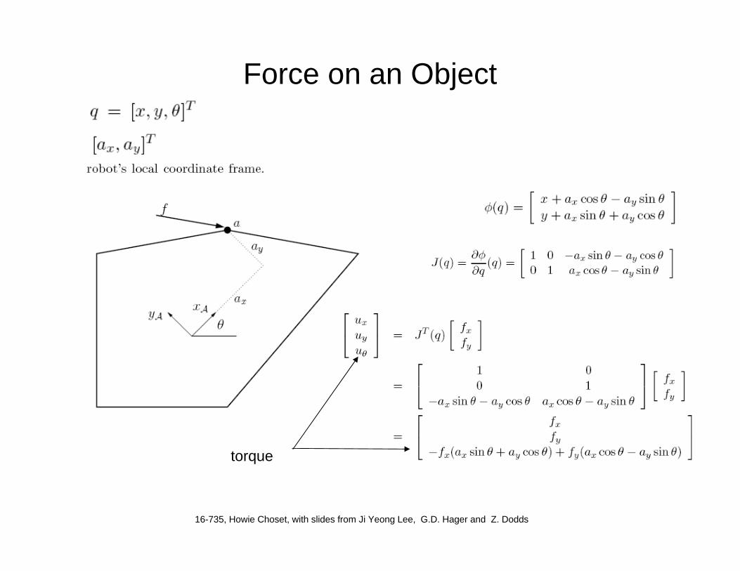
• Recall we can think of the gradient vectors as forces -- the basic idea is to define forces in the workspace (which is ℜ2 or ℜ3)
Power in configuration space
Power in work space
Power is conserved!
16-735, Howie Choset, with slides from Ji Yeong Lee, G.D. Hager and Z. Dodds
Force on an Object
torque

16-735, Howie Choset, with slides from Ji Yeong Lee, G.D. Hager and Z. Dodds
Potential Function on Rigid Body
Pick enough points to “pin down” robot (2 in plane)
More points please

16-735, Howie Choset, with slides from Ji Yeong Lee, G.D. Hager and Z. Dodds
Potential Fields for Multiple Bodies
• Recall we can think of the gradient vectors as forces -- the basic idea is to define forces in the workspace (which is ℜ2 or ℜ3)
– We have Jt f = u where f is in W and u is in Q– Thus, we can define forces in W and then map them to Q
– Example: our two-link manipulator
α
β
L1
L2
(x,y)
y
x
x L1cα L2cα+β
y L1sα L2sα+β
= +

16-735, Howie Choset, with slides from Ji Yeong Lee, G.D. Hager and Z. Dodds
Potential Fields on Non-Euclidean Spaces
– Example: our two-link manipulator
– J = - L1 sα - L2 sα+β - L2 sα+βL1 cα + L2 cα+β L2 cα+β
Suppose qgoal = (0,0)t, then fW = (x,y)
fq = x (- L1 sα - L2 sα+β) + y ( L1 cα + L2 cα+β)x (- L2 sα+β) + y L2 cα+β
α
β
L1
L2
(x,y)
y
x
x L1cα L2cα+β
y L1sα L2sα+β
= +

16-735, Howie Choset, with slides from Ji Yeong Lee, G.D. Hager and Z. Dodds
In General
• Pick several points on the manipulator
• Compute attractive and repulsive potentials for each
• Transform these into the configuration space and add
• Use the resulting force to move the robot (in its configuration space)
α
β
L1
L2
(x,y)
y
x
RF4
RF3
RF2
RF1
AF1
Be careful to use the correct Jacobian!

16-735, Howie Choset, with slides from Ji Yeong Lee, G.D. Hager and Z. Dodds
A Simulation Example
• Problem: simulate a planar n-link (revolute) manipulator.
• Kinematics: Let v(θ) = [cθ,sθ]t
• Points of revolution: p0 = [0,0]t αi = ∑ιj=1 θi
pi = pi-1 + Li v(αi)• Jacobian: w(θ) = [-sθ,cθ]t
Jn = Ln w(αn)Jn-1 = Jn + Ln-1 w(αn-1)
• Now, use the revolute points as the control points to generate force vectors (note this could lead to problems in some cases).

16-735, Howie Choset, with slides from Ji Yeong Lee, G.D. Hager and Z. Dodds
Summary
• Basic potential fields– attractive/repulsive forces
• Gradient following and Hessian
• Navigation functions
• Extensions to more complex manipulators