biomechanical models and robotic systems for human motion
TRANSCRIPT

Biomechanical Models and Robotic Systems for
Human Motion Assessment
Sarah Seko
Electrical Engineering and Computer SciencesUniversity of California, Berkeley
Technical Report No. UCB/EECS-2021-22
http://www2.eecs.berkeley.edu/Pubs/TechRpts/2021/EECS-2021-22.html
May 1, 2021

Copyright © 2021, by the author(s).All rights reserved.
Permission to make digital or hard copies of all or part of this work forpersonal or classroom use is granted without fee provided that copies arenot made or distributed for profit or commercial advantage and that copiesbear this notice and the full citation on the first page. To copy otherwise, torepublish, to post on servers or to redistribute to lists, requires prior specificpermission.

Biomechanical Models and Robotic Systems for Human Motion Assessment
by
Sarah Seko
A dissertation submitted in partial satisfaction of the
requirements for the degree of
Doctor of Philosophy
in
Engineering – Electrical Engineering and Computer Sciences
in the
Graduate Division
of the
University of California, Berkeley
Committee in charge:
Professor Ruzena Bajcsy, ChairProfessor Claire Tomlin
Professor Oliver O’Reilly
Spring 2020

Biomechanical Models and Robotic Systems for Human Motion Assessment
Copyright 2020by
Sarah Seko

1
Abstract
Biomechanical Models and Robotic Systems for Human Motion Assessment
by
Sarah Seko
Doctor of Philosophy in Engineering – Electrical Engineering and Computer Sciences
University of California, Berkeley
Professor Ruzena Bajcsy, Chair
Over the past several decades, there have been advances in the development of complexrobotic devices for daily assistance or rehabilitation. The use of such devices, however, haslargely remained limited to a research setting due to the prohibitive cost and required opera-tional engineering expertise. Likewise, dedicated biomechanics facilities perform quantitativemotion analysis, contrasting the qualitative and static imaging methods which are standardin clinical care. The aim of this dissertation is to develop and validate affordable methodsand devices for assessing and assisting human motion.
We first present a framework for improved estimation of whole-body human kinematicswith data from a single depth-camera. The algorithm incorporates biomechanical and dy-namic constraints for near-real time analysis of human motion. The approach is validatedagainst data from a ground-truth motion capture system on sit-to-stand (STS), an activityof daily living which requires significant torque generation and coordinated movement ofmultiple joints. We additionally present two methods for modeling the torso: a generalizedrelationship for the lower-lumbar angle and an optimization-based method for estimating asubject-specific model. Building on these modeling methods, we introduce a passive elasticknee orthotic device which provides bilateral knee assistance during STS. The device designand analysis integrate models of the human and device dynamics. Preliminary human sub-jects tests demonstrate a decrease in the human knee torque as well as positive changes inwhole-body biomechanics. Finally, we introduce an affordable planar robotic manipulandumfor upper limb assessment and assistance. The mechanical, electrical, and control architec-tures are presented, along with preliminary human subjects tests of reaching and ellipticaltrajectories with force field assistance under an admittance controller. A protocol for theassessment of strength and coordination is introduced and integrated with a biomechanicalmodel of the arm. With a total material cost of less than $800, this device provides anaccessible platform for clinical robotic assessment and rehabilitation.

i
To my parents, Raymon and Georgianna Seko, for their endless love, support, andencouragement.

ii
Contents
Contents ii
List of Figures iv
List of Tables x
1 Introduction 11.1 Thesis Overview and Contributions . . . . . . . . . . . . . . . . . . . . . . . 2
2 Depth Camera Motion Assessment 52.1 Overview of Clinical Motion Assessment . . . . . . . . . . . . . . . . . . . . 52.2 Rigid-Body Modeling Framework . . . . . . . . . . . . . . . . . . . . . . . . 82.3 Experimental Validation . . . . . . . . . . . . . . . . . . . . . . . . . . . . . 142.4 Algorithm Performance . . . . . . . . . . . . . . . . . . . . . . . . . . . . . . 192.5 Discussion . . . . . . . . . . . . . . . . . . . . . . . . . . . . . . . . . . . . . 242.6 Extension to Single-leg Squat . . . . . . . . . . . . . . . . . . . . . . . . . . 252.7 Chapter Summary . . . . . . . . . . . . . . . . . . . . . . . . . . . . . . . . 27
3 Recovering a Rigid-Body Model of the Spine 283.1 Torso Models in Motion Assessment . . . . . . . . . . . . . . . . . . . . . . . 283.2 Recovering a Functional Spine Model . . . . . . . . . . . . . . . . . . . . . . 293.3 Experimental Validation . . . . . . . . . . . . . . . . . . . . . . . . . . . . . 343.4 Discussion . . . . . . . . . . . . . . . . . . . . . . . . . . . . . . . . . . . . . 363.5 Chapter Summary . . . . . . . . . . . . . . . . . . . . . . . . . . . . . . . . 38
4 A Passively Assistive Knee Orthotic 394.1 Motivation and Overview . . . . . . . . . . . . . . . . . . . . . . . . . . . . . 394.2 Methods . . . . . . . . . . . . . . . . . . . . . . . . . . . . . . . . . . . . . . 414.3 Experiment . . . . . . . . . . . . . . . . . . . . . . . . . . . . . . . . . . . . 424.4 Biomechanical Effects of Assistance . . . . . . . . . . . . . . . . . . . . . . . 434.5 Chapter Summary . . . . . . . . . . . . . . . . . . . . . . . . . . . . . . . . 47
5 An Affordable Device for Robotic Therapy 49

iii
5.1 Overview of Upper Limb Rehabilitation Robotics . . . . . . . . . . . . . . . 505.2 Device Design . . . . . . . . . . . . . . . . . . . . . . . . . . . . . . . . . . . 515.3 Hardware Validation . . . . . . . . . . . . . . . . . . . . . . . . . . . . . . . 595.4 Admittance Control Framework . . . . . . . . . . . . . . . . . . . . . . . . . 615.5 Preliminary Human Subjects Experiments . . . . . . . . . . . . . . . . . . . 655.6 Simulation Case Study: Effect of Passive Flexor Muscle Tightness on Joint
Torques During Planar Arm Reaching . . . . . . . . . . . . . . . . . . . . . . 705.7 Chapter Summary . . . . . . . . . . . . . . . . . . . . . . . . . . . . . . . . 75
6 Algorithms for Assistance and Assessment 766.1 Exploitation of Assistance During Ellipse Tracing . . . . . . . . . . . . . . . 766.2 Spring Assistance Formulation . . . . . . . . . . . . . . . . . . . . . . . . . . 786.3 Experimental Protocol . . . . . . . . . . . . . . . . . . . . . . . . . . . . . . 816.4 Results . . . . . . . . . . . . . . . . . . . . . . . . . . . . . . . . . . . . . . . 826.5 Strength Assessment via Joint Motion Isolation . . . . . . . . . . . . . . . . 926.6 Chapter Summary . . . . . . . . . . . . . . . . . . . . . . . . . . . . . . . . 96
7 Final Thoughts and Future Work 98
Bibliography 100

iv
List of Figures
1.1 Thesis overview . . . . . . . . . . . . . . . . . . . . . . . . . . . . . . . . . . . 2
2.1 The three skeletal models. Left: Raw Kinect Skeleton. The joint centers obtainedfrom the Kinect are shown as crosses. The markers which are not used in thiswork are shown in the dashed blue. A cartoon outline of a subject is shownfor reference. Center: Model I: Floating Pelvis Rigid-body Model. The pelvisis defined as the base link, with three serial chain branches. The sequence ofrevolute joints are shown as cylinders. Right: Model II: Fixed-ankle Rigid-bodyModel. The right ankle is fixed to the ground and used as the base link. Therevolute joint sequence and segment lengths are the same as in the center figure. 9
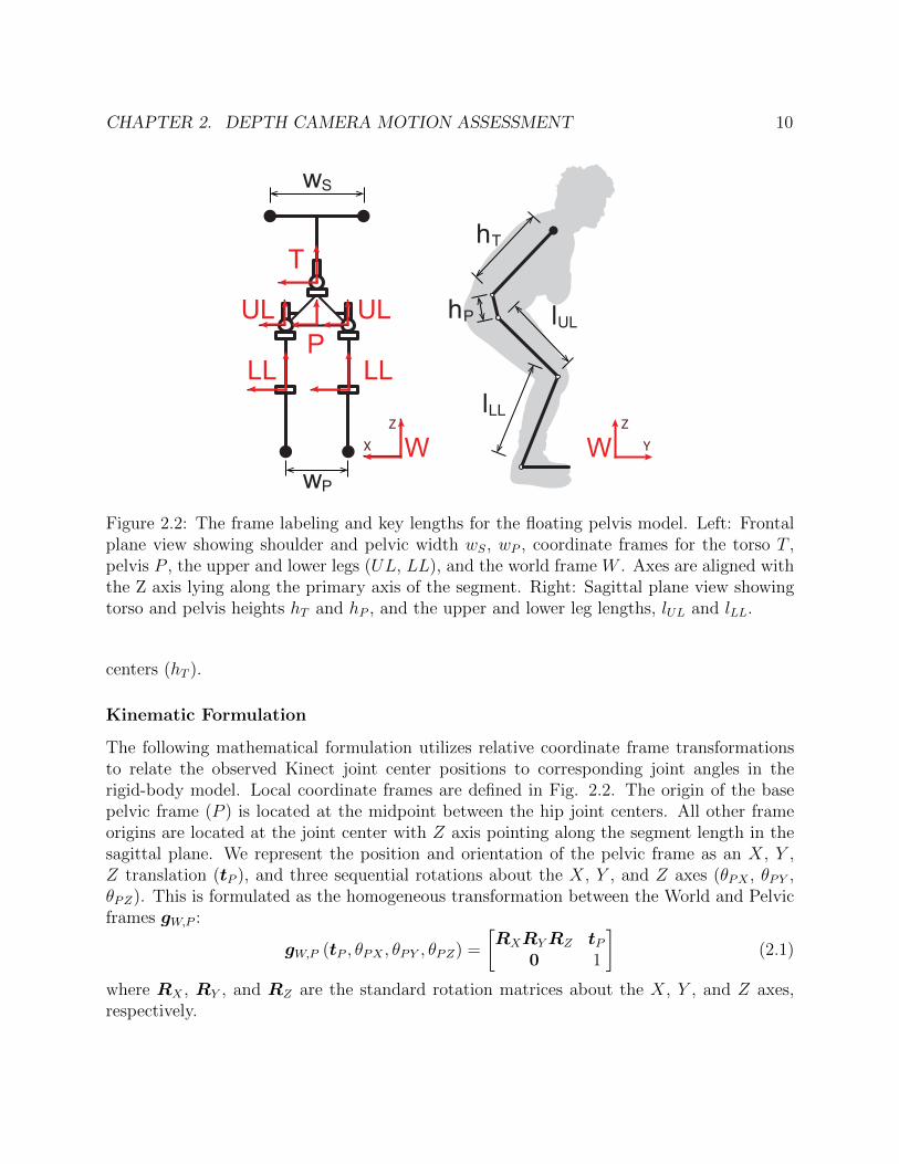
2.2 The frame labeling and key lengths for the floating pelvis model. Left: Frontalplane view showing shoulder and pelvic width wS, wP , coordinate frames for thetorso T , pelvis P , the upper and lower legs (UL, LL), and the world frame W .Axes are aligned with the Z axis lying along the primary axis of the segment.Right: Sagittal plane view showing torso and pelvis heights hT and hP , and theupper and lower leg lengths, lUL and lLL. . . . . . . . . . . . . . . . . . . . . . 10
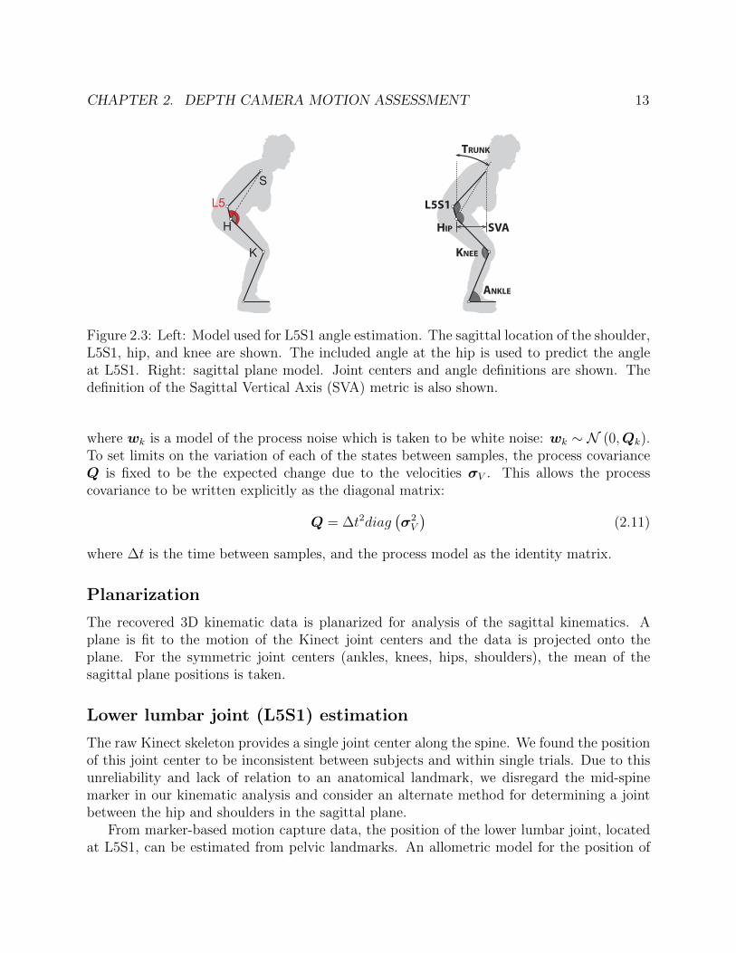
2.3 Left: Model used for L5S1 angle estimation. The sagittal location of the shoulder,L5S1, hip, and knee are shown. The included angle at the hip is used to predictthe angle at L5S1. Right: sagittal plane model. Joint centers and angle definitionsare shown. The definition of the Sagittal Vertical Axis (SVA) metric is also shown. 13
2.4 Linear regression for L5S1, the angle formed by the knee, hip, and L5S1, joints,from KHS, the angle formed by the knee, hip, and shoulder joints. The model isshown in solid black. Data from the test set of 6 subjects is shown in dotted color. 15
2.5 Motion capture marker protocol used in this work. Markers (red) are shownsuperimposed on the standard Plug-in-Gait model. . . . . . . . . . . . . . . . . 16
2.6 Left: Torso and pelvis frames are highlighted, with markers shown as crosses,and joint centers shown as circles. Right: Segment-marker definitions used forNLS recovery. The sagittal view of the torso frame, and caudal view of the pelvisframe are shown. Torso markers were located at the Incisura jugularis sternalis(IJ), Xiphoid Process (XP), and at the C7 and T8 spinous processes which werefound during standing. Pelvis markers were located at the right and left AnteriorSuperior Iliac Spines (ASIS) and Posterior Superior Iliac Spines (PSIS). . . . . 17
v
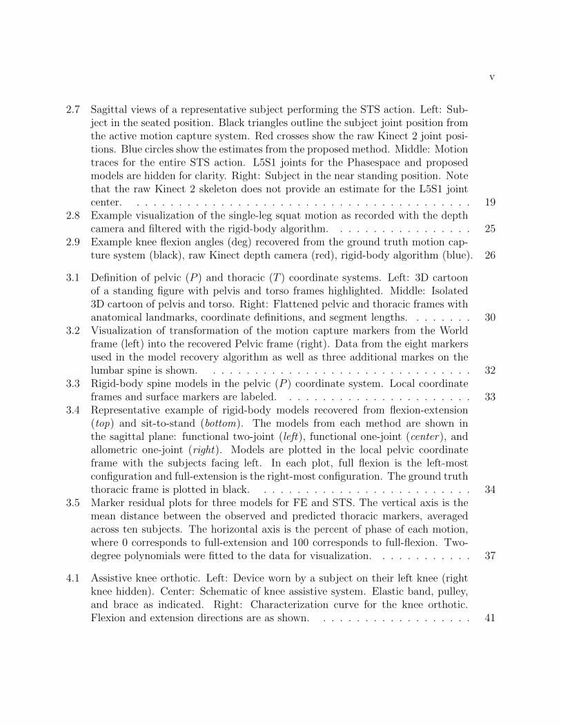
2.7 Sagittal views of a representative subject performing the STS action. Left: Sub-ject in the seated position. Black triangles outline the subject joint position fromthe active motion capture system. Red crosses show the raw Kinect 2 joint posi-tions. Blue circles show the estimates from the proposed method. Middle: Motiontraces for the entire STS action. L5S1 joints for the Phasespace and proposedmodels are hidden for clarity. Right: Subject in the near standing position. Notethat the raw Kinect 2 skeleton does not provide an estimate for the L5S1 jointcenter. . . . . . . . . . . . . . . . . . . . . . . . . . . . . . . . . . . . . . . . . 19
2.8 Example visualization of the single-leg squat motion as recorded with the depthcamera and filtered with the rigid-body algorithm. . . . . . . . . . . . . . . . . 25
2.9 Example knee flexion angles (deg) recovered from the ground truth motion cap-ture system (black), raw Kinect depth camera (red), rigid-body algorithm (blue). 26
3.1 Definition of pelvic (P ) and thoracic (T ) coordinate systems. Left: 3D cartoonof a standing figure with pelvis and torso frames highlighted. Middle: Isolated3D cartoon of pelvis and torso. Right: Flattened pelvic and thoracic frames withanatomical landmarks, coordinate definitions, and segment lengths. . . . . . . . 30
3.2 Visualization of transformation of the motion capture markers from the Worldframe (left) into the recovered Pelvic frame (right). Data from the eight markersused in the model recovery algorithm as well as three additional markes on thelumbar spine is shown. . . . . . . . . . . . . . . . . . . . . . . . . . . . . . . . 32
3.3 Rigid-body spine models in the pelvic (P ) coordinate system. Local coordinateframes and surface markers are labeled. . . . . . . . . . . . . . . . . . . . . . . 33
3.4 Representative example of rigid-body models recovered from flexion-extension(top) and sit-to-stand (bottom). The models from each method are shown inthe sagittal plane: functional two-joint (left), functional one-joint (center), andallometric one-joint (right). Models are plotted in the local pelvic coordinateframe with the subjects facing left. In each plot, full flexion is the left-mostconfiguration and full-extension is the right-most configuration. The ground truththoracic frame is plotted in black. . . . . . . . . . . . . . . . . . . . . . . . . . 34
3.5 Marker residual plots for three models for FE and STS. The vertical axis is themean distance between the observed and predicted thoracic markers, averagedacross ten subjects. The horizontal axis is the percent of phase of each motion,where 0 corresponds to full-extension and 100 corresponds to full-flexion. Two-degree polynomials were fitted to the data for visualization. . . . . . . . . . . . 37
4.1 Assistive knee orthotic. Left: Device worn by a subject on their left knee (rightknee hidden). Center: Schematic of knee assistive system. Elastic band, pulley,and brace as indicated. Right: Characterization curve for the knee orthotic.Flexion and extension directions are as shown. . . . . . . . . . . . . . . . . . . 41

vi
4.2 Knee torque during sit-to-stand as a function of time (left) and knee angle (right).Each plot has three lines for the assistive mode: the resultant torque from thehuman and device (red), the device torque (black), and the remaining humantorque (green). Additionally, the human torque in the unassistive mode is plot-ted in blue. The trace represents the mean trajectory across all trials with thestandard deviation shown as a shaded region of the same colour. The plots areshown for each subject and separated by the natural foot (top row) and anteriorfoot placement (bottom row) conditions. . . . . . . . . . . . . . . . . . . . . . 44
4.3 Trajectory of the center of mass (COM) of the head-arms-trunk segment duringSTS with natural foot placement (top) and anterior foot placement (bottom).Trajectories are normalized by subject height with the average taken across alltrials for each subject. Blue lines denote assisted trajectory and Red lines denoteunassisted trajectory. . . . . . . . . . . . . . . . . . . . . . . . . . . . . . . . . 45
4.4 Vertical linear momentum of the head-arms-trunk segment. Unassisted motionis shown in red dashed line with assisted motion in blue solid line. The valuesare normalized by subject height and mass and shown for S01 (left) and S02(right) under the natural foot placement (top row) and anterior foot placement(bottom row). In each plot, the mean over 21 motions is shown with the standarddeviation in shaded bounds. . . . . . . . . . . . . . . . . . . . . . . . . . . . . 46
5.1 Examples of upper-limb robotic rehabilitation devices. A: In-Motion Arm, thecommercial version of the MIT-MANUS [84], B: ARMin 4 [85], C: H-Man [86],D: NeRoBot [87]. . . . . . . . . . . . . . . . . . . . . . . . . . . . . . . . . . . 50
5.2 Subject seated in front of upper-limb planar rehabilitation device . . . . . . . . 525.3 Diagram of the mechanical structure of the robot . . . . . . . . . . . . . . . . . 535.4 CAD model of the wrist platform (left) and interior force system (right) . . . . 555.5 Top-down view of the force system . . . . . . . . . . . . . . . . . . . . . . . . . 565.6 Electronic system architecture . . . . . . . . . . . . . . . . . . . . . . . . . . . 575.7 Diagram of the motor electronics subsystem . . . . . . . . . . . . . . . . . . . . 585.8 Diagram of the force measurement electronics subsystem . . . . . . . . . . . . . 585.9 Sample data comparing the position trajectories as measured by the ground truth
motion capture system and robotic device in the x-direction (top) and y-direction(middle). The error in both directions is shown on the bottom plot. . . . . . . 59
5.10 Sample data comparing the force trajectories as measured by the ground truthforce/torque sensor and robotic device in the x-direction (top) and y-direction(middle). The error in both directions is shown on the bottom plot. . . . . . . 60
5.11 Block diagram of the admittance control framework . . . . . . . . . . . . . . . 615.12 Rigid body models of the upper limb. Left: 5-dof model with a spherical shoulder
joint, a cylindrical joint for elbow flexion/extension, and a cylindrical joint forwrist pronantion/supination. Right: planar 2-dof model of the arm with cylin-drical joints at the shoulder and elbow for flexion/extension. . . . . . . . . . . 63

vii
5.13 Figures illustrating the steps to solve to the inverse kinematics problem for the5-dof upper-limb model. Step 0 shows the initial reference configuration for thearms. Figures 1 - 5 show the steps outlined in the text. . . . . . . . . . . . . . 64
5.14 Assistive glove . . . . . . . . . . . . . . . . . . . . . . . . . . . . . . . . . . . . 655.15 Top-down view of planar reaching trajectories for control (left), post-stroke (cen-
ter), and PLS (right) subjects. The color of each line corresponds to the velocityof the wrist at that point. Subjects performed series of reaches from the home po-sition to radially placed targets. The subject’s reachable workspace as measuredby clinician is depicted in gray. . . . . . . . . . . . . . . . . . . . . . . . . . . . 67
5.16 Preliminary observations from the human subject protocol. Top left: represen-tative velocity plots for a single reaching motion for control subject (purple),post-stroke subject (blue), and subject with Primary Lateral Sclerosis (Red).Bottom left: demonstration of feasibility to identify key stages of grasp duringa reach-to-grasp motion. Right: representative trajectory for a forward reachingmotion for a control subject (left) and a post-stroke subject (right), illustratinginability to stabilize at the trajectory endpoint. . . . . . . . . . . . . . . . . . . 68
5.17 Bar charts showing mean peak force (left) and mean peak velocity (right) forhealthy controls subejcts completing reaching trials under the different admit-tance controller virtual dynamics. Peak force and velocity values are normalizedto the subject mean. Values represents the mean across the subjects with theerror bar corresponding to inter-subject variance. The admittance mode virtualdynamics were defined by the following parameters: A1) m = 3.3 kg, αv = 0.25,A2) m = 3.3 kg, αv = 0.5 A3) m = 2.2 kg, αv = 0.5. . . . . . . . . . . . . . . . 69
5.18 Left: representative reaching data from a subject with spinal cord injury under-going passive reaching to three radial targets. Wrist position is shown in blackwith the interaction force shown as the scaled red vector. Right: musculosketalarm model. Figure from [101]. . . . . . . . . . . . . . . . . . . . . . . . . . . . 71
5.19 (Left) Passive muscle force vs. muscle length. Relationship is shown for fourvalues of nominal muscle length l0. (Right) Simulated wrist positions for reachingtrajectories in Cartesian space. . . . . . . . . . . . . . . . . . . . . . . . . . . . 71
5.20 Kinematic configuration at three arm configurations along reaching trajectoriesin the left, center, and right directions. Arm links are shown in black with flexormuscles in red and extensor muscles in blue. The reaching trajectory is shown asthe dashed line. . . . . . . . . . . . . . . . . . . . . . . . . . . . . . . . . . . . 73
5.21 Resultant maximum torques at the elbow (top row) and shoulder (bottom row)for muscle tightness conditions. The nomical muscle length L1 corresponds to theshortest muscle length, with L4 being the greatest. Torques are plotted as themaximum value for a given reaching angle defined in the Cartesian space betweenthe wrist position and the horizontal line through the center point. . . . . . . . 74

viii
6.1 Sample of the data from preliminary experiment demonstrating subject leaninginto force field during reaching. (Left) Top-down view of reaching trajectories totargets at 0, 45, and 90 degrees from the vertical. The velocity at the point isrepresented by the color. (Right) Sampled interaction force overlaid on top ofreaching trajectory. . . . . . . . . . . . . . . . . . . . . . . . . . . . . . . . . . 77
6.2 Left: drawing of the tangent-normal coordinate frame for linear spring assistance,showing the unit and normal tangent vectors, un and ut, current position p anddesired position d. Right: plot of the vector field of the linear spring assistancefor a linear desired trajectory. . . . . . . . . . . . . . . . . . . . . . . . . . . . 78
6.3 Illustration of the method for determining the unit tangent vector ut and unitnormal vectorun at a point p when tracking an elliptical trajectory. (Left) Findingthe desired point d, (Center) Computing the unit tangent and unit normal vectorsat the desired position, (Right) Translating the tangent-normal coordinate frameto the current position. . . . . . . . . . . . . . . . . . . . . . . . . . . . . . . . 80
6.4 Vector field plot of the assistive spring force field for an elliptical trajectory.Arrows indicated the magnitude and direction of the force for the given positionerror from the desired trajectory. . . . . . . . . . . . . . . . . . . . . . . . . . . 82
6.5 Subject connected to rehabilitation device. The monitor displays the desiredtrajectory and real-time feedback of the subject’s wrist position. . . . . . . . . 83
6.6 Illustration of the interaction force decomposition (Left) and the heading error(Right) . . . . . . . . . . . . . . . . . . . . . . . . . . . . . . . . . . . . . . . . 84
6.7 Representative data for a subject completing elliptical trajectories under unas-sisted (left column) and assisted (right column) admittance control. Top row:The end-effector (wrist) position is plotted with the color corresponding to thevelocity at that point. The end-effector force is shown in the solid black arrowswith arrow length and direction corresponding to the magnitude and directionof the interaction force. Bottom Row: The normal component of the force, fn isplotted in the red arrows. . . . . . . . . . . . . . . . . . . . . . . . . . . . . . . 86
6.8 Bar charts of the results of of ellipse tracking, showing the mean normalized force(left), mean normalized duration (center), and mean heading error. . . . . . . . 87
6.9 Example plots of normal force for an unconstrained (red) and constrained (blue)trials. . . . . . . . . . . . . . . . . . . . . . . . . . . . . . . . . . . . . . . . . . 89
6.10 Example plots for a subject completing unconstrained elliptical tracing withcolumns corresponding to the four orientations measured with respect to thevertical. Top Row: plots of trajectory with interaction force overlaid as blackarrows. Center row: joint angles for the shoulder (blue) and elbow (red) joints.Bottom row: joint torques estimated from inverse statics analysis for the shoulder(blue) and elbow (red). . . . . . . . . . . . . . . . . . . . . . . . . . . . . . . . 90
ix
6.11 Example plots of segmenting ellipse tracking into phases of elbow and shoulderflexion or extension. Estimated mean joint elbow and shoulder torques are shownfor an ellipse tracing trial. The background shading relates whether each joint isexerting a torque in flexion (F) or extension (E). The labels indicate the elbowstatus followed by the shoulder (e.g. FE indicates elbow flexion and shoulderextension). . . . . . . . . . . . . . . . . . . . . . . . . . . . . . . . . . . . . . . 91
6.12 Illustration of the joint motion isolation protocol with elbow isolation on the leftand shoulder isolation on the right. . . . . . . . . . . . . . . . . . . . . . . . . 93
6.13 Visualization of the motion capture data from the joint isolation trials of theelbow joint (left) and shoulder joint (right). . . . . . . . . . . . . . . . . . . . . 93
6.14 Example plots of the end effector forces measured during the joint isolation pro-tocol for flexion and extension of the elbow and shoulder joints. . . . . . . . . . 95
6.15 Estimated joint torques for shoulder (blue) and elbow (red) joints during elbowisolation (left) and shoulder isolation (right). Each plot shows the mean for threetrials with the standard deviation shaded. . . . . . . . . . . . . . . . . . . . . . 96
x
List of Tables
2.1 Inter-rater assessments for estimated joint position. Mean absolute error (MAE),concordance correlation coefficient (CCC) and interclass correlation coefficient(ICC) are given for each skeletal joint. Mean absolute errors are stated as a meanwith the standard deviation in parenthesis. Ankle correlation coefficients for thefixed-ankle model are omitted as the ankle position in this model does not varywith time. . . . . . . . . . . . . . . . . . . . . . . . . . . . . . . . . . . . . . . 20
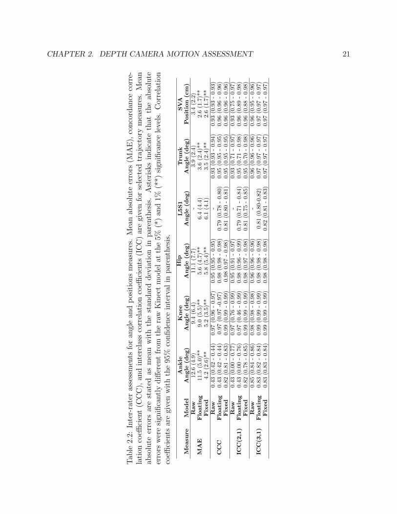
2.2 Inter-rater assessments for angle and positions measures. Mean absolute errors(MAE), concordance correlation coefficient (CCC), and interclass correlation co-efficients (ICC) are given for selected trajectory measures. Mean absolute errorsare stated as mean with the standard deviation in parenthesis. Asterisks indicatethat the absolute errors were significantly different from the raw Kinect modelat the 5% (*) and 1% (**) significance levels. Correlation coefficients are givenwith the 95% confidence interval in parenthesis. . . . . . . . . . . . . . . . . . 21
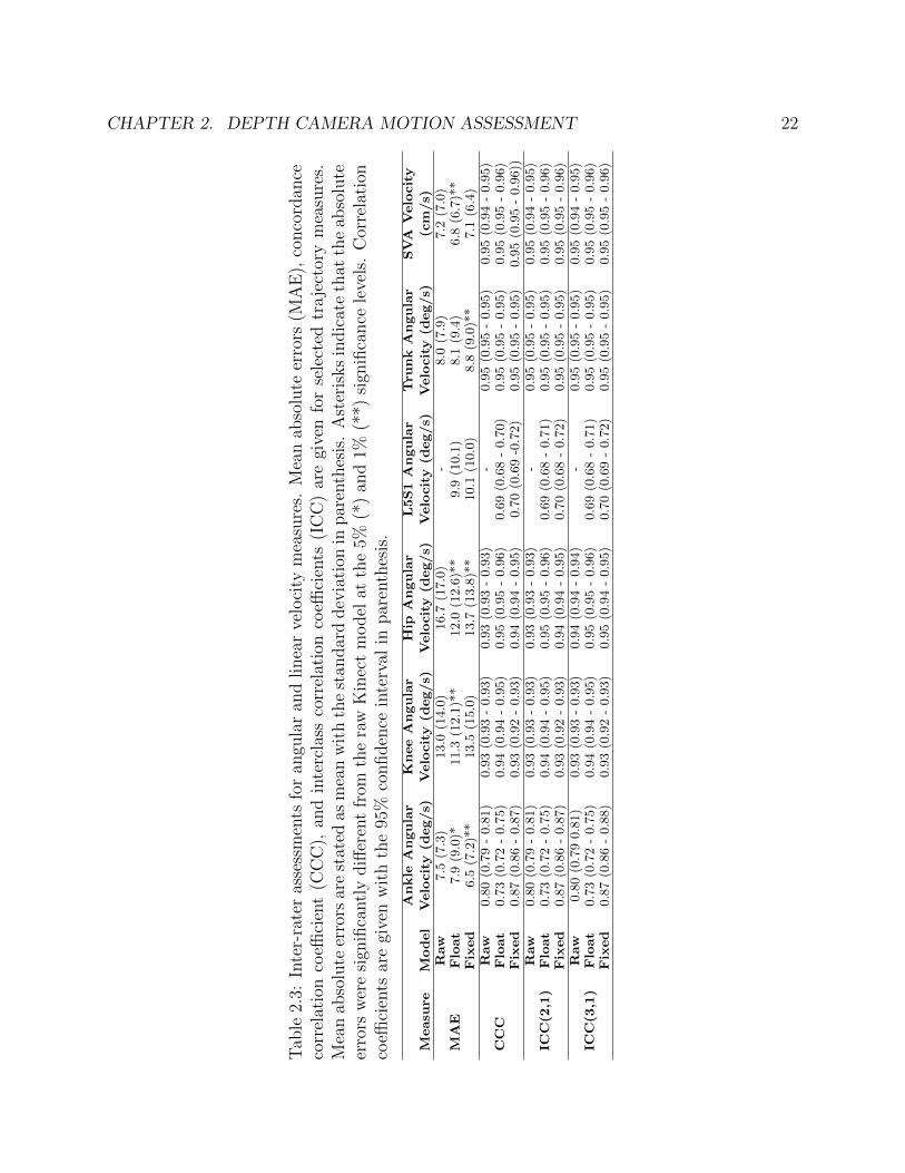
2.3 Inter-rater assessments for angular and linear velocity measures. Mean absoluteerrors (MAE), concordance correlation coefficient (CCC), and interclass correla-tion coefficients (ICC) are given for selected trajectory measures. Mean absoluteerrors are stated as mean with the standard deviation in parenthesis. Asterisksindicate that the absolute errors were significantly different from the raw Kinectmodel at the 5% (*) and 1% (**) significance levels. Correlation coefficients aregiven with the 95% confidence interval in parenthesis. . . . . . . . . . . . . . . 22
2.4 Inter-rater assessments for peak measures. The angle at L5S1 is modeled usingthe author’s proposed method. Mean absolute errors (MAE), concordance cor-relation coefficient (CCC), and interclass correlation coefficients (ICC) are givenfor selected trajectory measures. Mean Absolute Errors are stated as mean withthe standard deviation in parenthesis. Asterisks indicate that the absolute er-rors were significantly different from the raw Kinect model at the 5% (*) and 1%(**) significance levels. Correlation coefficients are given with the 95% confidenceinterval in parenthesis. . . . . . . . . . . . . . . . . . . . . . . . . . . . . . . . 23
3.1 Parameter and state constraints for one-joint (left) and two-joint (right) models. 353.2 Mean thoracic marker residuals (mm) for functional and allometric models. Bolded
entries indicate models trained and tested on the same motion (different data set). 36
xi
3.3 Mean recovered parameters for functional models. Values represent the parameteras a percentage of subject height. . . . . . . . . . . . . . . . . . . . . . . . . . . 36
6.1 Quantitative interaction metrics under four virtual dynamic conditions: LightUnassisted (LU), Light Assisted (LA), Heavy Unassisted (HU), and Heavy As-sisted (HA). The mean is taken across all subjects with the standard deviationcorresponding to variance across subjects. . . . . . . . . . . . . . . . . . . . . . 87
6.2 Mean force for each subject under four virtual dynamic conditions: Light Unas-sisted, Light Assisted, Heavy Unassisted, and Heavy Assisted. The mean andstandard deviation are taken across all trials for the condition (all orientations). 87
xii
Acknowledgments
This work would not have been possible without the support of my collaborators andcommunity. Firstly, I would like to thank my research advisor, Professor Ruzena Bajcsy,for giving me the freedom to explore my research interests, asking tough questions, andsupporting me throughout my PhD. I would also like to thank my dissertation commit-tee members, Professors Claire Tomlin and Oliver O’Reilly, as well as my qualifying examcommittee member Professor Karunesh Ganguly.
I am grateful for the research insights and kindness that have been given to me by themembers of the Human Assistive Robotic Technologies (HART) Lab. I would especially liketo thank Robert Peter Matthew, who has been my closest collaborator and friend throughoutmy time at Berkeley. My additional co-authors who contributed directly to this dissertationinclude Raziel Riemer, Jeffrey Lotz, and Joel Loeza. I would additionally like to thankGregorij Kurillo, Louis Cheng, Brian Feeley, Jeannie Bailey, and Patrick Curran for feedbackon the clinical depth-camera framework, and Adelyn Tu-Chan and Karunesh Ganguly forinsight into the design of the upper-limb assistive device. Special thanks go to Shirley Salanioand Jessica Gamble for their friendly support in stressful times.
Finally, I would like to thank all of my family, friends, and teachers who have supportedand encouraged me throughout my education.
This dissertation includes research supported by the Office of Naval Research EmbeddedHumans MURI Award (N000141310341), the National Science Foundation SBIR Award(1R41AR068202-01A1), and the SanDisk Fellowship.
1
Chapter 1
Introduction
Motion of the human body is achieved through the complex and coordinated control of theelements of the musculoskeletal system by the central nervous system. Typical biomechanicalfunction can be disrupted by neuromusculoskeletal injury or disease resulting in deficits inareas such as strength, coordination, and range of motion. These decreases in motor functionaffect the ability to complete activities of daily living (ADLs), fundamental actions necessaryto care for oneself independently [1].
The quantitative assessment of motoric ability and impairment is useful for diagnosis, re-covery tracking, and the prescription of medical intervention and treatment. Human motionanalysis utilizes quantitative methods for tracking kinematics and developing biomechanicalmodels, estimating internal forces and torques during movement. These methods often relyon sophisticated and expensive motion capture technology, which require specialized facili-ties and expertise. The clinical standard of care does not typically incorporate these tools,relying on qualitative and subjective measures of motion or static medical imaging.
The field of assistive or rehabilitation robotics is inherently connected to motion assess-ment, providing technologies for both collecting quantitative data of human motion andadministering assistance. These devices mechanically connect to the subject, enabling mea-surement of interactions forces which can inform biomechanical models. Additionally, quan-titative assessment of a subject’s ability or performance can drive individualized modelsor therapy protocols. Despite significant engineering advances in the field of rehabilitationrobotics over the last decades, we have not seen a widespread implementation of these com-plex robotic mechanisms in clinical or home care. While several factors inhibit the adoptionof rehabilitation robotics, an undeniable barrier results from high device cost and complexity.This inaccessibility further contributes to a limited understanding of models of recovery andoptimal robotic rehabilitation protocols.

CHAPTER 1. INTRODUCTION 2
Figure 1.1: Thesis overview
1.1 Thesis Overview and Contributions
The focus of this dissertation is the development and validation of affordable methods anddevices for assessing and assisting human motion with the future aim of translation to clinicalor home settings. We utilize tools from rigid-body modeling, kinematic and dynamic analysis,optimization, and interaction control. An emphasis is placed on empirical validation throughhardware characterization and human subjects studies which compare our technologies toground truth measures. The organization and key contributions of the thesis are summarizedbelow and shown in Figure 1.1.
Human Motion Analysis (Chapters 2 and 3)
We first present a framework for accurate and fast recovery of joint kinematics using asingle-depth camera [2]. This method incorporates biomechanical and dynamical constraintsinto the recovery of joint kinematics from unconstrained joint center positions measured bya depth camera. Our method is validated on 10 subjects completing sit-to-stand (STS),an ADL and action of clinical interest. When compared against a gold-standard, marker-based, motion capture system, our method was found to produce accurate, reproducible, andconsistent estimates of joint center positions and kinematics. The single depth camera canbe used in a clinical or home space with a total test time of less than one minute and nearreal-time processing, providing an affordable and fast tool for clinical motion assessment.
CHAPTER 1. INTRODUCTION 3
While it was applied to STS and the single-leg squat motions, the method is extendable toother motions.
In whole-body motion analysis, the human torso is often modeled as a single rigid seg-ment. More detailed modeling of the low back allows for the analysis of posture and loadingon the spine. In Chapter 1, we present a method for a generalized relationship for the lum-bosacral joint position. We expand on this in Chapter 2 with a method for estimating asubject-specific model of joint positions from observed marker-based motion data [3]. Thisoptimization-method builds on existing functional methods for joint center recovery. Wecompare models generated from human subjects during sit-to-stand and a flexion-extensionmotion against a model generated from an allometrically-scaled measurement. An analysisof the marker residuals finds that the proposed functional models have lower residuals andphase-dependency, indicating a better fit for the analysis of torso kinematics.
Passive Knee Assistance (Chapter 4)
Building on our work in biomechanical modeling, we present a novel passive knee orthoticwhich provides bilateral knee extension assistance during STS [4]. This device utilizes anelastic element to store energy when the knee is flexed during sitting which is released duringstanding. By modeling the device and human kinematics and dynamics, we study the effectof single-joint assistance on the control strategy adopted by human subjects. We find thatassistance results in a decrease in the human knee torque as well as changes in whole-bodybiomechanics, notably an increase in the linear momentum of the upper body and a decreasein the anterior excursion of the center of mass. These results indicate that single-jointassistance at the knee has the potential to both facilitate successful STS and positively alterwhole-body biomechanics.
Active Upper Limb Assistance (Chapters 5 and 6)
Finally, we present the design, analysis, and validation of a planar robotic manipulandumfor upper limb assessment and assistance. Connected at the wrist, the device enables end-effector control of the human arm, operating under position and velocity control as well asforce-based admittance control for volitional motion. The device can move the arm through alarge workspace with resistive and assistive forces applied along linear or curved trajectories.The mechanical, electrical, and control systems are presented, along with preliminary humansubjects tests of reaching trajectories in a control population with case study data from twosubjects with upper-limb impairment. We present a novel solution for 3-D upper limb inversekinematic recovery, utilizing the device constraints. A 2-D model and a simple 6-musclemodel of the upper limb are also discussed. Hardware validation and initial human subjectresults demonstrate device accuracy and functionality. We note differences in the interactionforce, trajectory smoothness and velocity, and ability to stabilize between control subjectsand subjects with upper-limb impairment .

CHAPTER 1. INTRODUCTION 4
In Chapter 6, we explore two algorithms for upper-limb assessment with the device de-tailed in Chapter 5: 1) the exploitation of assistive spring force-fields in tracking an ellipticaltrajectory and 2) the assessment of strength and coordination through isolated joint motion.These new methods demonstrate additional device functionality.

5
Chapter 2
Depth Camera Motion Assessment
The study of joint kinematics and dynamics has broad clinical applications including theidentification of pathological motions or compensation strategies and the analysis of dynamicstability. High-end motion capture systems, however, are expensive and require dedicatedcamera spaces with lengthy set-up and data processing commitments. Depth cameras, suchas the Microsoft Kinect, provide an inexpensive, marker-free alternative at the sacrifice ofjoint-position accuracy. In this work, we present a fast framework for adding biomechanicalconstraints to the joint estimates provided by a depth camera system. We also present anew model for the lower lumbar joint angle. We validate key joint position, angle, andvelocity measurements against a gold standard active motion-capture system on ten healthysubjects performing sit-to-stand (STS). Our method showed significant improvement in MeanAbsolute Error (MAE) and Intraclass Correlation Coefficients (ICC) for the recovered jointangles and position-based metrics. These improvements suggest that depth cameras canprovide an accurate and clinically viable method of rapidly assessing the kinematics andkinetics of the STS action, providing data for further analysis using biomechanical or machinelearning methods.
2.1 Overview of Clinical Motion Assessment
Musckuloskeletal disorders of the spine and knee lead to approximately 39 million visitsto clinical care facilities each year in the United States [5]. Despite the prevalence of theseconditions, there remains a lack of scalable, accessible, and quantitative assessments for wholebody biomechanics in clinic. The current clinical gold standard for documenting functionalspine impairment is the measurement of Cobb angles in flexion and extension [6, 7], orthe Sagittal Vertical Axis (SVA) from radiographs [8]. Such radiographs are inexpensiveand offer a precise measurement of vertebral range of motion, but they only assess staticpostures. During daily functional activities such as sit-to-stand (STS), the strategy used tostand can vary [9, 10, 11], potentially changing the loads experienced by the joints. Thisresults in both inconsistencies in patient care throughout the recovery process and challenges

CHAPTER 2. DEPTH CAMERA MOTION ASSESSMENT 6
in understanding the relationship between static observations and functional abilities.Full-body motion analysis can provide insight into pathological motions and compensa-
tion strategies. This analysis is performed in biomechanics labs using gold-standard tech-niques such as motion capture, force platforms, and surface electromyography. This data canbe processed using full-body biomechanics software such as Anybody [12] or OpenSIM [13].While these systems are a staple in obtaining high resolution kinematic, force, and muscularmeasurements, their application to regular clinical practice is limited by the time requiredto setup these measurements, the cost of the equipment, required expertise, and the needfor a dedicated motion-capture space.
This has resulted in a dichotomy in analysis, with patients assessed with static measuresfocused at a particular body segment, while biomechanical labs are able to track and analyzethe dynamic motion of the whole-body. Some researchers have explored the use of special-ized wearable sensing systems for tracking spine function. Marras developed an exoskeletaltracking system for the lumbar spine to identify motions during occupational tasks, and toidentify differences in individuals with low back pain [14, 15]. This system was shown toprovide a quantitative kinematic measure of dysfunction based on a specific set of flexiontasks. Taylor and Consmuller developed a system for non-invasive back measurement usingflexible strain gauges to measure the curvature of the spine [16, 17]. This system was shownto provide a reliable quantitative assessment of spine shape and range of motion when com-pared to X-ray. While these systems have been shown to provide good estimates of spinemotion and can discriminate between pain and asymptomatic subjects, as they only trackspine motion, they are not able to assess changes in full-body motion.
Depth cameras such as the Microsoft Kinect have been used as a marker-less methodfor assessing function. Unlike the prior motion capture strategies, no hardware (markers,sensors etc.) needs to be attached to the subject. This allows for rapid testing and sim-plifies clinical deployment. One of the disadvantages of the use of depth cameras is themethod used to identify subject landmarks. As no markers are placed on the subject, thelocation of a subject’s joint centres (Fig 2.1) relies on machine learning to label the pixelscorresponding to each body segment. The intersection between body segments is then takento be the estimated joint location [18]. This form of joint centre data from a depth cam-era is not unique to the Kinect; alternative depth camera sensors (Orbec, Intel RealSense,VicoVR, Depthsense, PMD, SIC), as well as skeletal tracking systems (Nuitrack, OpenNI)are commercially available. As there is no underlying rigid-body model, the estimated jointcentres may be biologically inconsistent. This can lead to errors at the ankle, knee, and hipwhich complicate the use of depth sensors for later analysis [19]. Researchers have foundthat retro-reflective markers could be used to supplement the recovery process [20]. Theaddition of these markers adds to the experiment setup time, and sensitivity to the accuracyof marker placement.
An important distinction between this work and the work performed in the computervision community is the underlying assumptions and goals of the final system. We developa tool for rapid clinical assessment by applying a biomechanically realistic model to imposeconstraints on unconstrained estimates of joint position for a controlled task and environ-

CHAPTER 2. DEPTH CAMERA MOTION ASSESSMENT 7
ment. In contrast, the problem tackled by a number of these other works are the estimationof human poses across a wide range of tasks while being robust to real-world situations andenvironments [21].
Two approaches are generally taken when performing pose estimation: creating a skeletalmodel with a prior on the associated surface geometry, or the generation of a direct mapbetween camera inputs and pose using machine learning. Pavlakos [22] uses convolutionalneural networks to estimate the likelihood that a voxel contains a joint. This method resultedin an average 3D joint error of 9.6 cm for the Human3.6M sitting down motion and an averagemarker reconstruction error of 5 cm. This outperforms a number of other deep learningmethods [23, 24] yet still highlights the inherent challenges in joint estimation, particularlyin self-occluding tasks such as sitting. This is consistent with the work by Mehta [25] whoadopted a similar approach at the pixel level providing a real time (30 fps) system, but witha mean joint position error of 14-15 cm for the sit-down task. While these methods offera promising method for versatile estimation of human motion, the current joint estimationerror is high relative to the surface fitting methods.
Surface fitting methods usually use a simplified approximation of human shape, consistingof scaled cylinders or ellipsoids that are adjusted to a subjects body morphology. Thissimplified model is then used to estimate pose by relating these volumes to camera depthdata. Recent advances have involved the use of Gaussian models to approximate body shape[26], with Ding [27] developing a method that can estimate joint centre position at 20 fps withan associated position error of 3.5 cm. Shuai [28] used spherical harmonic decompositionrather than Gaussians to track subjects with multiple depth cameras. The resulting modelexhibited low marker re-projection error, though this error increased in actions with selfocclusion such as sitting. Zhang [18] used a full-body skinned mesh model in conjunctionwith multiple depth cameras and force sensing shoes to estimate kinematic and dynamicstate. The resulting system was slow, but accurate with a mean joint error of 3.8 cm at6 fps. Unfortunately no results were published for any sitting or standing actions, but theauthors do state the the system performance did decrease on self-occluding activities. Thelower errors and potential for these methods to run in real time suggests that these methodsmay be suitable for clinical use, but the need for initial calibration of the shape modelby performing an explicit calibration motion [26, 18, 27] or through manual labelling [28]detracts from their use. Similarly, the use of multiple cameras suggests a requirement of adedicated motion capture space where the system can be setup and left undisturbed betweensessions.
Contributions
In this chapter, we assesses the feasibility of using a single depth camera as a clinical assess-ment tool for whole-body kinematic and kinetic assessment. As such, we prioritize:
1. Accurate anatomical joint center locations and joint angles which are needed for clinicalassessment and future dynamic/musculoskeletal modeling.

CHAPTER 2. DEPTH CAMERA MOTION ASSESSMENT 8
2. Fast computation time to allow for immediate review by the clinician.
3. Ease of use by non-specialists in a clinical environment to perform a rapid motionassessment.
To these aims, we present a simple, fast method for taking any pre-estimated joint centerlocations, automatically scaling skeletal parameters based on the subject height and recov-ering kinematic and kinetic measures from the biomechanical model. This system providesaccurate, reproducible, and consistent estimates of anatomical joint center locations, with amean joint position error of 2.63 cm. An additional estimate of L5S1 location is added to thekinematic model allowing for assessment of the lower back, an important site of analysis inclinical and occupational health scenarios. The proposed system is used as a post-processingstep on the raw Kinect 2 skeleton, with the mean computation speed of 524 frames per sec-ond. This suggests this method can be incorporated into many existing real-time methodswithout a significant drop in frame-rate. Only a single RGB-D camera is used, allowing fordeployment clinical space without the need of a dedicated, calibrated motion capture space.The extraction of kinematic states is performed only requiring the user to specify the sub-ject’s height, without any manual model tuning, or joint labeling. The entire time to setupthe camera, coach the subject to perform the STS action, data collection, and kinematicrecovery takes under 1 minute.
2.2 Rigid-Body Modeling Framework
Rigid-body models are commonly used in biomechanics research to estimate joint kinematicsand loading [29, 30, 31, 32, 33]. The mathematical formulations for the kinematics, kinetics,and dynamics of these systems can be taken from the robotics literature [34], providing aversatile method for analyzing arbitrary rigid-body systems. In this work, we present andevaluate two rigid-body models:
1. Floating pelvis rigid-body model : constrained body segment lengths. This form ofmodel is typically used in motion analysis, with no environmental constraints.
2. Fixed-ankle rigid-body model : constrained body segment lengths and angle-groundcontact. As the ankles do not move in the sit-to-stand action, a kinematic constrainton ankle position can be used to determine the effect on the recovered kinematic andkinetic measures.
The models are driven by the raw Kinect shoulder, hip, knee, and ankle joint center positions.

CHAPTER 2. DEPTH CAMERA MOTION ASSESSMENT 9
Raw Kinect
Model
Floating Pelvis
Model
Fixed Ankle
Model
Figure 2.1: The three skeletal models. Left: Raw Kinect Skeleton. The joint centers obtainedfrom the Kinect are shown as crosses. The markers which are not used in this work are shownin the dashed blue. A cartoon outline of a subject is shown for reference. Center: Model I:Floating Pelvis Rigid-body Model. The pelvis is defined as the base link, with three serialchain branches. The sequence of revolute joints are shown as cylinders. Right: Model II:Fixed-ankle Rigid-body Model. The right ankle is fixed to the ground and used as the baselink. The revolute joint sequence and segment lengths are the same as in the center figure.
Model I: Floating pelvis rigid-body model
Model structure
The human body is commonly modeled as a floating tree system, consisting of a pelvic base-link with serial chains that terminate at the head, hands, and feet [35]. In this work, westudy the kinematics of the lower limbs and trunk during STS, neglecting the motion of thearms. We consider a 3D rigid-body model with six segments: (left and right) lower leg, (leftand right) upper leg, pelvis, and torso (Figure 2.1). The corresponding joint centers are atthe ankle, knee, hip, and lower-lumbar joints. The knee joint is modeled as a cylindricaljoint. The ankles, hips, and lower-lumbar (L5S1) joint are modeled as spherical joints withthree successive rotations. The order of these rotations is based on relations to commonrange of motion measures [36].
Segment lengths are determined by recommended height-scaled, sex-specific, allometricrelations [37]. These relations provide estimated link length for the upper and lower leg, (lUL
and lLL), shoulder width and hip width, (wS and wP ), the length between the midpoint ofthe hip centers and L5S1 (hP ) and the length between L5S1 and midpoint of the shoulder
CHAPTER 2. DEPTH CAMERA MOTION ASSESSMENT 10
hP
hT
lUL
lLL
wS
wP
Z
X
Z
YW W
LL
UL
P
T
UL
LL
Figure 2.2: The frame labeling and key lengths for the floating pelvis model. Left: Frontalplane view showing shoulder and pelvic width wS, wP , coordinate frames for the torso T ,pelvis P , the upper and lower legs (UL, LL), and the world frame W . Axes are aligned withthe Z axis lying along the primary axis of the segment. Right: Sagittal plane view showingtorso and pelvis heights hT and hP , and the upper and lower leg lengths, lUL and lLL.
centers (hT ).
Kinematic Formulation
The following mathematical formulation utilizes relative coordinate frame transformationsto relate the observed Kinect joint center positions to corresponding joint angles in therigid-body model. Local coordinate frames are defined in Fig. 2.2. The origin of the basepelvic frame (P ) is located at the midpoint between the hip joint centers. All other frameorigins are located at the joint center with Z axis pointing along the segment length in thesagittal plane. We represent the position and orientation of the pelvic frame as an X, Y ,Z translation (tP ), and three sequential rotations about the X, Y , and Z axes (θPX , θPY ,θPZ). This is formulated as the homogeneous transformation between the World and Pelvicframes gW,P :
gW,P (tP , θPX , θPY , θPZ) =
[RXRYRZ tP
0 1
](2.1)
where RX , RY , and RZ are the standard rotation matrices about the X, Y , and Z axes,respectively.

CHAPTER 2. DEPTH CAMERA MOTION ASSESSMENT 11
The relative transformations between each adjacent segment are defined in the samenotation. For example, the transformation between the Pelvis and Torso (T ) frames, gP,Tcan be written:
gP,T (hP , θTX , θTY , θTZ) =
RXRYRZ
00hP
0 1
(2.2)
using the coordinate frames and segment lengths defined in Figure 2.2.These homogeneous pose matrices are used to estimate the World frame locations of the
left and right shoulder centers from their local positions and relative frame transformations:
[psho left psho right
1 1
]= gW,PgP,T
−wS
0hT1
+wS
0hT1
(2.3)
This process can be repeated for each joint center to create the observation model for alljoints:
psho left
psho right
phip left
phip right
pknee left
pknee right
pankle left
pankle right
= hobs (η,X) (2.4)
where η are the model parameters:
η =[hP , hT , lUL, lLL, wS, wP
](2.5)
and XI ∈ R17 is the state vector containing the corresponding translations and rotations:
XI =[tP ,θP ,θT ,θUL left,θUL right,
θLL left, θLL right]T (2.6)
Model II: Rigid-body model with fixed-ankle
Our second rigid-body model introduces an additional constraint by fixing the position ofthe ankle joint centers. The raw joint centers from the depth camera are not constrainedby the ground plane, allowing the ankle to phase through the floor or hover above the floorwhile the person is standing. During STS, we assume the position of the ankle remainsfixed and can be constrained at a fixed position throughout the motion. To implement thisconstraint, we select the base link to be one of the feet and fix this position to the ground.

CHAPTER 2. DEPTH CAMERA MOTION ASSESSMENT 12
The mathematical formulation of the observation model is similar to Section 2.2, with themodel starting at one foot and moving up the leg, before branching at the pelvis into thetorso and second leg branches.
The state vector XII ∈ R14 for the fixed ankle model has three fewer states whencompared to the floating pelvis model, with the addition of the ipsilateral ankle rotationθA ipsi ∈ R3 and the removal of the pelvis translation and orientation (R6):
XII =[θA ipsi, θLL ipsi,θUL ipsi,θUL contra,
θLL contra,θT ]T(2.7)
where the subscripts ipsi and contra refer to the ipsilateral and contralateral sides to thebase foot.
In our model, the ankle joint center is fixed at a position based on the observed motion.The X and Z coordinates are taken to be the mean observed position throughout the motion.The Y coordinate is fixed to be equal to the mean anterior-posterior position of the knee ata standing posture.
Inverse Kinematics
The kinematic recovery process allows for the estimation of joint angles from observationsof joint position. We use two methods of kinematic recovery are: Non-linear Least Squares(NLS) and Unscented Kalman Filtering (UKF).
Non-linear Least Squares (NLS)
The error between the observed joint centers q and the expected joint centers hobs (η,X) isminimized for each frame k:
minXk
‖qk − hobs (η,Xk)‖22 (2.8)
Unscented Kalman Filtering (UKF)
While the NLS method allows for the estimation of the state at each frame, it does not enforceany relationship between sequential states. The UKF balances inaccuracies in measurementwith an estimate of the change in state between two successive states [38, 39]. Using thenotation for Kalman filters, every observed joint center at frame k can be written:
qk = hobs(η, Xk
)+ vk (2.9)
where vk is a model of the sensor noise which is taken to be white noise: vk ∼ N (0,Rk),Rk is the covariance matrix of the Kinect, and the state Xk is the true state that underlieseach observation.
This observation model is combined with a process model fproc which relates previousestimates of the the true state Xk−1 to the current true state:
Xk = fproc(Xk−1
)+wk (2.10)
CHAPTER 2. DEPTH CAMERA MOTION ASSESSMENT 13
S
H
K
L5
TRUNK
SVA
ANKLE
KNEE
HIP
L5S1
Figure 2.3: Left: Model used for L5S1 angle estimation. The sagittal location of the shoulder,L5S1, hip, and knee are shown. The included angle at the hip is used to predict the angleat L5S1. Right: sagittal plane model. Joint centers and angle definitions are shown. Thedefinition of the Sagittal Vertical Axis (SVA) metric is also shown.
where wk is a model of the process noise which is taken to be white noise: wk ∼ N (0,Qk).To set limits on the variation of each of the states between samples, the process covarianceQ is fixed to be the expected change due to the velocities σV . This allows the processcovariance to be written explicitly as the diagonal matrix:
Q = ∆t2diag(σ2
V
)(2.11)
where ∆t is the time between samples, and the process model as the identity matrix.
Planarization
The recovered 3D kinematic data is planarized for analysis of the sagittal kinematics. Aplane is fit to the motion of the Kinect joint centers and the data is projected onto theplane. For the symmetric joint centers (ankles, knees, hips, shoulders), the mean of thesagittal plane positions is taken.
Lower lumbar joint (L5S1) estimation
The raw Kinect skeleton provides a single joint center along the spine. We found the positionof this joint center to be inconsistent between subjects and within single trials. Due to thisunreliability and lack of relation to an anatomical landmark, we disregard the mid-spinemarker in our kinematic analysis and consider an alternate method for determining a jointbetween the hip and shoulders in the sagittal plane.
From marker-based motion capture data, the position of the lower lumbar joint, locatedat L5S1, can be estimated from pelvic landmarks. An allometric model for the position of
CHAPTER 2. DEPTH CAMERA MOTION ASSESSMENT 14
L5S1 in a pelvic frame is presented in Reed et al. [40] Unfortunately, the pelvic orientationis not observable from the Kinect data, so we cannot apply this method.
A model for lumbosacral orientation using knee flexion and trunk inclination is presentedby Anderson et al. [41]. In that work, a quadratic model was trained on four subjects inmultiple static lifting postures. This model was not assessed on any test data. Using activemotion capture data, we tested the Anderson model against the marker-based Reed method.We found that the model did not accurately predict the sacral orientation during STS.
In this work, we present a new regression model for KHL5, the angle formed by the knee,hip, and L5S1 joints, driven by KHS, the angle formed by the knees, hips, and shoulders(joints present in the Kinect data). This model assumes that coordination between the hipand L5S1 joints follows a predictable pattern across subjects.
The model is trained using marker-based motion capture data (protocol detailed in Sec-tion 2.3). We define the pelvic frame by anterior and posterior superior iliac spine (ASISand PSIS) markers shown in Fig. 2.5. The location of the L5S1 joint center is based onthe model presented in Reed, in which the L5S1 joint center in given a frame defined by theASIS and pubic symphysis (PS) landmarks. The PS landmark is not possible to mark on aclothed subject or easily observable from motion capture data. Using dry pelvis data fromReynolds, et al. [42], we re-derived the position of the L5S1 joint in the ASIS-PSIS pelvicframe:
L5S1 =[0 0 .11PW
]T(2.12)
where the pelvic width PW is the distance between the left and right ASIS landmarks. Fromthe observed L5S1 joint center, we compute the joint angles in the sagittal plane. A linearmodel was fit to the data:
KHL5 = αSHK + β (2.13)
with derived model parameters α = 0.82, β = 0.54 and r-squared 0.9784. This modelwas trained on four subjects performing STS and tested against six subjects. Each subjectperformed STS three times. The fitted model and test data are shown in Fig. 2.4. Themean absolute error (MAE) between the predicted and observed L5S1 angles was 3.63±1.72degrees for the test set 4.21± 2.73 degrees for the training set.
From Eq. 2.13 and an allometrically scaled pelvic height, hp, we can express the positionof the L5S1 joint center. In our recovery framework, this L5S1 model is used after thekinematic recovery and planarization steps are performed.
2.3 Experimental Validation
The modeling and kinematic recovery methods introduced in Section 2.2 were tested exper-imentally and validated against marker-based motion capture data on non-clinical subjects.

CHAPTER 2. DEPTH CAMERA MOTION ASSESSMENT 15
60 80 100 120 140 160 180 200 220
Knee-Hip-Shoulder Angle (degrees)
100
120
140
160
180
Kne
e-H
ip-L
5S1
Ang
le (
degr
ees)
ModelTest Data
Figure 2.4: Linear regression for L5S1, the angle formed by the knee, hip, and L5S1, joints,from KHS, the angle formed by the knee, hip, and shoulder joints. The model is shown insolid black. Data from the test set of 6 subjects is shown in dotted color.
Experimental Protocol
Ten subjects (3F/7M, age: 30.9 ± 9.6, height: 1.76 ± 0.12 m, mass: 67.4 ± 11.2 kg) wererecruited under informed consent (UCSF IRB 16-21015). Subjects wore close fitting exerciseclothing (sports bra, exercise shorts). The chair height was adjusted so that the subject’sthighs were parallel to the ground, and their knees directly above their ankles during naturalsitting. Subjects were asked to perform STS with their arms folded across their chest, handstouching the opposite elbow. The standing action was otherwise non-coached, with subjectsperforming the action naturally. Three trials, each consisting of three STS, were recordedfor each subject.
Active Motion Capture Model
An 8-camera active motion capture system was used in this study to provide a ground-truth estimate of position and orientation of each body segment. Motion data of STS wassimultaneously recorded from the Kinect and the motion capture system. The Kinect camera

CHAPTER 2. DEPTH CAMERA MOTION ASSESSMENT 16
Figure 2.5: Motion capture marker protocol used in this work. Markers (red) are shownsuperimposed on the standard Plug-in-Gait model.
was located 2.5 meters directly in-front of the subject. The Kinect joint centers were streamedat 30Hz and saved with a UNIX timestamp onto a desktop computer. Each trial consisted of883± 87 frames of Kinect depth data, and 14224± 1548 frames of Phasespace data for threesuccessive stand-sit-stand motions (around 30 seconds). The Kinect and motion capturesystems were time synchronized using a network time protocol server.
Thirty-two LED markers (Phasespace, San Leandro, CA) were recorded at 480Hz withan associated UNIX timestamp. Kinematic recovery was performed offline in MATLAB. Themarkers were placed onto the subjects skin using adhesive Velcro® based on the Plug-in-Gaitmarkers set [43] (Figure 2.5). Additional markers were placed on the medial elbow, knee,and ankle positions to allow for estimates of joint center from the medio-lateral marker pairs.In cases where the subject’s shorts or sports bra obscured the ASIS, PSIS, or XP landmarks,

CHAPTER 2. DEPTH CAMERA MOTION ASSESSMENT 17
lC7Y
l T8Y
l Torso
lPelv
lPSIS
lASIS
lC7Z
l T8Z
C7
T8
IJ
XP
RPSIS
RASIS
LPSIS
LASIS
Z
Y
Y
X
Figure 2.6: Left: Torso and pelvis frames are highlighted, with markers shown as crosses,and joint centers shown as circles. Right: Segment-marker definitions used for NLS recovery.The sagittal view of the torso frame, and caudal view of the pelvis frame are shown. Torsomarkers were located at the Incisura jugularis sternalis (IJ), Xiphoid Process (XP), and atthe C7 and T8 spinous processes which were found during standing. Pelvis markers werelocated at the right and left Anterior Superior Iliac Spines (ASIS) and Posterior SuperiorIliac Spines (PSIS).
a clip was used to secure the marker to the clothes band at the desired landmark.In addition to the STS protocol, a data set was collected for identifying the functional
joint centers for each segment using the Recap2 protocol. Subjects were asked to moveeach joint through its full range of motion three times, starting with the wrists, elbows, andshoulders, before moving the ankles, knees, and hips. The Recap2 protocol was only used tofind the functional centers for the ground truth motion capture model.
NLS (Section 2.2) was used to recover the instantaneous position and orientation of eachlimb segment in 3D coordinates. Each limb segment was recovered independently withoutany modeling of the connection between connected limbs.
The rigid-body models used for each each segment are shown in Figure 2.6. The coordi-nate system is based on Wu [44], with the exception of the pelvis segment where the origin islocated at the midpoint of the ASIS and PSIS markers. The labeling of the coordinate axeswere also modified to simplify plotting and analysis in MATLAB. NLS was used to estimatethe marker positions in the local coordinate frame for each subject.

CHAPTER 2. DEPTH CAMERA MOTION ASSESSMENT 18
The joint centers for the ground-truth model were recovered using functional methods(hip and shoulder), and marker-based methods (ankle, knee, and L5S1). Geometric spherefitting for the hip was chosen based on the recommendation by the ISB [44] and as all subjectswere able to move sufficiently [45]. The inter-malleolar point was selected for the ankles fromWu [44], the inter-epicondyle point for the knee [46], and L5S1 from the allometric modeldescribed in Section 2.2. The recovered joint-centers were planarized and the relative angleswere determined at each frame.
Data Analysis
All data processing was performed on previously stored Kinect 2 data on an Intel i7-5820Kprocessor, with 32GB of RAM running Windows 7 Enterprise. Each trial of three stand-sit-stand actions consisted of roughly 880 frames and was post-processed at 524 ± 140 fps. Agraphics card was not used to aid computation.
The joint angles recovered from each method were filtered and numerically differentiatedto obtain joint velocity estimates. A first-order, low-pass Butterworth filter at 5 Hz wasapplied to the active motion capture and both rigid-body Kinect models [47, 48]. The rawkinect data was filtered more heavily, using a first-order low-pass Butterworth filter at 2 Hz.This was to account for significant noise in the raw joint angles leading to unrealistic velocityestimates.
We compute the horizontal distance between the shoulder joint and hip joint centers ateach frame as well as its velocity. This is a surrogate for the Sagittal Vertical Axis (SVA), ametric for spinal alignment, measured by static radiographs as the distance between C7 andL5S1 [8]. We also compare recovered peak values for several metrics during STS: flexion andextension velocities of the torso, torso inclination angle, and SVA.
We consider each combination of sensor and model (raw Kinect, floating rigid-bodyKinect, fixed-ankle rigid-body Kinect, and active motion capture) to be a different rater,allowing for the use of inter-rater reliability assessment methods. Three statistical measureswere used to analyze the performance of the raw and rigid-body Kinect models against theactive motion capture ground truth:
1. Absolute Error (MAE) identifies the raw position or velocity error between meth-ods.
2. Lin’s Concordance Correlation Coefficient (CCC) assesses inter-rater reliabilitybetween methods [49]
3. Inter-class Correlations Coefficients (ICC) identifies the absolute agreement(ICC(2,1)) and relative consistency (ICC(3,1)) between methods [50, 51, 52]. ICCvalues were interpreted as poor (< 0.4), fair (0.4− 0.59), good (0.6− 0.74), and excel-lent (≥ 0.75) based on the treatment by [53, 54].

CHAPTER 2. DEPTH CAMERA MOTION ASSESSMENT 19
2.4 Algorithm Performance
MAE, CCC, and ICC statistics are given for joint center positions (Table 2.1), joint trajec-tories (Table 2.2), velocity trajectories (Table 2.3), and selected peak metrics (Table 2.4). Arepresentative motion capture trace is shown in Figure 2.7.
-0.4 -0.2 0 0.2
0
0.5
1
1.5
-0.4 -0.2 0 0.2
0
0.5
1
1.5
-0.4 -0.2 0 0.2
0
0.5
1
1.5
Anteroposterior Position (m)
Cra
nio
ca
ud
al P
ositio
n (
m)
Figure 2.7: Sagittal views of a representative subject performing the STS action. Left:Subject in the seated position. Black triangles outline the subject joint position from theactive motion capture system. Red crosses show the raw Kinect 2 joint positions. Blue circlesshow the estimates from the proposed method. Middle: Motion traces for the entire STSaction. L5S1 joints for the Phasespace and proposed models are hidden for clarity. Right:Subject in the near standing position. Note that the raw Kinect 2 skeleton does not providean estimate for the L5S1 joint center.
Both rigid-body Kinect models (floating and fixed-ankle) achieved significantly lowerMAE than the raw Kinect for all joint angle and position measures (Tables 2.1, 2.2). Incomparison to the floating model, the fixed-ankle model had significantly less error in theankle and knee positions and angles, and comparable error in all other measures.
Higher CCC and ICC values indicate greater reliability, relative consistency, and absoluteagreement. For the position measures, the fixed-ankle model has higher CCC and ICC valuesthan the raw Kinect in all cases. The floating pelvis model was better than the raw Kinectmodel, but has poor performance in recovering the ankle positions and angle.

CHAPTER 2. DEPTH CAMERA MOTION ASSESSMENT 20
Tab
le2.
1:In
ter-
rate
ras
sess
men
tsfo
res
tim
ated
join
tp
osit
ion.
Mea
nab
solu
teer
ror
(MA
E),
conco
rdan
ceco
rrel
atio
nco
effici
ent
(CC
C)
and
inte
rcla
ssco
rrel
atio
nco
effici
ent
(IC
C)
are
give
nfo
rea
chsk
elet
aljo
int.
Mea
nab
solu
teer
rors
are
stat
edas
am
ean
wit
hth
est
andar
ddev
iati
onin
par
enth
esis
.A
nkle
corr
elat
ion
coeffi
cien
tsfo
rth
efixed
-ankle
model
are
omit
ted
asth
ean
kle
pos
itio
nin
this
model
does
not
vary
wit
hti
me.
Ankle
Position
KneePosition
Hip
Position
ShoulderPosition
Measu
reM
odel
XY
XY
XY
XY
MAE
(cm)
Raw
8.66±
3.17
2.01±
1.69
1.96±
1.69
3.57±
2.38
1.93±
1.95
4.07±
2.44
1.98±
1.38
4.05±
2.04
Floating
8.31±
3.21
1.95±
1.59
1.88±
1.26
1.46±
1.42
2.40±
1.69
2.36±
1.28
1.71±
1.57
2.93±
2.11
Fixed
1.62±
0.07
1.97±
1.29
1.30±
1.08
0.78±
0.62
1.98±
1.36
2.07±
1.27
1.58±
1.28
3.08±
1.97
CCC
Raw
0.24
0.03
0.95
0.62
0.98
0.95
0.98
0.97
Floating
0.26
0.04
0.96
0.88
0.98
0.98
0.98
0.98
Fixed
--
0.97
0.97
0.99
0.99
0.99
0.98
ICC(2
,1)
Raw
0.24
0.03
0.95
0.62
0.98
0.95
0.98
0.97
Floating
0.26
0.04
0.96
0.88
0.98
0.98
0.98
0.98
Fixed
--
0.97
0.97
0.99
0.99
0.99
0.98
ICC(3
,1)
Raw
0.72
0.05
0.95
0.62
0.99
0.99
0.99
0.99
Floating
0.73
0.05
0.96
0.91
0.99
0.99
0.99
0.99
Fixed
--
0.97
0.97
0.99
0.99
0.99
0.99
CHAPTER 2. DEPTH CAMERA MOTION ASSESSMENT 21
Tab
le2.
2:In
ter-
rate
ras
sess
men
tsfo
ran
gle
and
pos
itio
ns
mea
sure
s.M
ean
abso
lute
erro
rs(M
AE
),co
nco
rdan
ceco
rre-
lati
onco
effici
ent
(CC
C),
and
inte
rcla
ssco
rrel
atio
nco
effici
ents
(IC
C)
are
give
nfo
rse
lect
edtr
aje
ctor
ym
easu
res.
Mea
nab
solu
teer
rors
are
stat
edas
mea
nw
ith
the
stan
dar
ddev
iati
onin
par
enth
esis
.A
ster
isks
indic
ate
that
the
abso
lute
erro
rsw
ere
sign
ifica
ntl
ydiff
eren
tfr
omth
era
wK
inec
tm
odel
atth
e5%
(*)
and
1%(*
*)si
gnifi
cance
leve
ls.
Cor
rela
tion
coeffi
cien
tsar
egi
ven
wit
hth
e95
%co
nfiden
cein
terv
alin
par
enth
esis
.
Measu
reM
odel
Ankle
Angle
(deg)
Knee
Angle
(deg)
Hip
Angle
(deg)
L5S1
Angle
(deg)
Tru
nk
Angle
(deg)
SVA
Position
(cm)
MAE
Raw
12.6
(4.9)
9.4
(6.4)
11.1
(7.7)
-3.9
(2.4)
3.4
(2.2)
Floating
11.5
(5.0)**
9.0
(5.5)**
5.6
(4.7)**
6.4
(4.4)
3.6
(2.4)**
2.6
(1.7)**
Fixed
4.2
(2.6)**
5.2
(3.5)**
5.8
(5.4)**
6.1
(4.1)
3.5
(2.4)**
2.6
(1.7)**
CCC
Raw
0.43(0.42-0.44)
0.97(0.96-0.97)
0.95(0.95-0.95)
-0.93(0.93-0.94)
0.93(0.93-0.93)
Floating
0.43(0.42-0.44)
0.97(0.97-0.97)
0.98(0.98-0.98)
0.79(0.78-0.80)
0.95(0.95-0.95)
0.96(0.96-0.96)
Fixed
0.82(0.81-0.83)
0.99(0.99-0.99)
0.980.97-0.98)
0.81(0.80-0.81)
0.95(0.95-0.95)
0.96(0.96-0.96)
ICC(2
,1)
Raw
0.43(0.00-0.77)
0.97(0.76-0.99)
0.95(0.91-0.97)
-0.93(0.71-0.97)
0.93(0.75-0.97)
Floating
0.43(0.00-0.76)
0.97(0.46-0.99)
0.98(0.96-0.99)
0.79(0.71-0.84)
0.95(0.71-0.98)
0.96(0.89-0.98)
Fixed
0.82(0.78-0.85)
0.99(0.99-0.99)
0.98(0.97-0.98)
0.81(0.75-0.85)
0.95(0.70-0.98)
0.96(0.88-0.98)
ICC(3
,1)
Raw
0.85(0.84-0.86)
0.98(0.98-0.98)
0.96(0.96-0.96)
-0.96(0.96-0.96)
0.96(0.95-0.96)
Floating
0.83(0.82-0.84)
0.99(0.99-0.99)
0.98(0.98-0.98)
0.81(0.80-0.82)
0.97(0.97-0.97)
0.97(0.97-0.97)
Fixed
0.83(0.83-0.84)
0.99(0.99-0.99)
0.98(0.98-0.98)
0.82(0.81-0.83)
0.97(0.97-0.97)
0.97(0.97-0.97)
CHAPTER 2. DEPTH CAMERA MOTION ASSESSMENT 22
Tab
le2.
3:In
ter-
rate
ras
sess
men
tsfo
ran
gula
ran
dlinea
rve
loci
tym
easu
res.
Mea
nab
solu
teer
rors
(MA
E),
conco
rdan
ceco
rrel
atio
nco
effici
ent
(CC
C),
and
inte
rcla
ssco
rrel
atio
nco
effici
ents
(IC
C)
are
give
nfo
rse
lect
edtr
aje
ctor
ym
easu
res.
Mea
nab
solu
teer
rors
are
stat
edas
mea
nw
ith
the
stan
dar
ddev
iati
onin
par
enth
esis
.A
ster
isks
indic
ate
that
the
abso
lute
erro
rsw
ere
sign
ifica
ntl
ydiff
eren
tfr
omth
era
wK
inec
tm
odel
atth
e5%
(*)
and
1%(*
*)si
gnifi
cance
leve
ls.
Cor
rela
tion
coeffi
cien
tsar
egi
ven
wit
hth
e95
%co
nfiden
cein
terv
alin
par
enth
esis
.
Measu
reM
odel
Ankle
Angular
Velocity
(deg/s)
KneeAngular
Velocity
(deg/s)
Hip
Angular
Velocity
(deg/s)
L5S1Angular
Velocity
(deg/s)
Tru
nk
Angular
Velocity
(deg/s)
SVA
Velocity
(cm/s)
MAE
Raw
7.5
(7.3)
13.0
(14.0)
16.7
(17.0)
-8.0
(7.9)
7.2
(7.0)
Float
7.9
(9.0)*
11.3
(12.1)**
12.0
(12.6)**
9.9
(10.1)
8.1
(9.4)
6.8
(6.7)**
Fixed
6.5
(7.2)**
13.5
(15.0)
13.7
(13.8)**
10.1
(10.0)
8.8
(9.0)**
7.1
(6.4)
CCC
Raw
0.80(0.79-0.81)
0.93(0.93-0.93)
0.93(0.93-0.93)
-0.95(0.95-0.95)
0.95(0.94-0.95)
Float
0.73(0.72-0.75)
0.94(0.94-0.95)
0.95(0.95-0.96)
0.69(0.68-0.70)
0.95(0.95-0.95)
0.95(0.95-0.96)
Fixed
0.87(0.86-0.87)
0.93(0.92-0.93)
0.94(0.94-0.95)
0.70(0.69-0.72)
0.95(0.95-0.95)
0.95(0.95-0.96))
ICC(2
,1)
Raw
0.80(0.79-0.81)
0.93(0.93-0.93)
0.93(0.93-0.93)
-0.95(0.95-0.95)
0.95(0.94-0.95)
Float
0.73(0.72-0.75)
0.94(0.94-0.95)
0.95(0.95-0.96)
0.69(0.68-0.71)
0.95(0.95-0.95)
0.95(0.95-0.96)
Fixed
0.87(0.86-0.87)
0.93(0.92-0.93)
0.94(0.94-0.95)
0.70(0.68-0.72)
0.95(0.95-0.95)
0.95(0.95-0.96)
ICC(3
,1)
Raw
0.80(0.790.81)
0.93(0.93-0.93)
0.94(0.94-0.94)
-0.95(0.95-0.95)
0.95(0.94-0.95)
Float
0.73(0.72-0.75)
0.94(0.94-0.95)
0.95(0.95-0.96)
0.69(0.68-0.71)
0.95(0.95-0.95)
0.95(0.95-0.96)
Fixed
0.87(0.86-0.88)
0.93(0.92-0.93)
0.95(0.94-0.95)
0.70(0.69-0.72)
0.95(0.95-0.95)
0.95(0.95-0.96)

CHAPTER 2. DEPTH CAMERA MOTION ASSESSMENT 23
Table 2.4: Inter-rater assessments for peak measures. The angle at L5S1 is modeled usingthe author’s proposed method. Mean absolute errors (MAE), concordance correlation coef-ficient (CCC), and interclass correlation coefficients (ICC) are given for selected trajectorymeasures. Mean Absolute Errors are stated as mean with the standard deviation in paren-thesis. Asterisks indicate that the absolute errors were significantly different from the rawKinect model at the 5% (*) and 1% (**) significance levels. Correlation coefficients are givenwith the 95% confidence interval in parenthesis.
Measure ModelPeak Trunk
Flexion Angle (deg)Peak SVA
Position (cm)
Peak TrunkFlexion Angular
Velocity (deg/s)
Peak TrunkExtension Angular
Velocity (deg/s)
Typical Value
Mocap 61.8 (4.9) 24.1 (3.6) 73.3 (10.0) 55.4 (10.8)Raw 60.4 (3.5) 25.1 (2.9) 58.8 (11.0) 50.5 (7.2)
Floating 57.6 (6.2) 24.5 (4.1) 76.3 (17.0) 65.1 (15.4)Fixed 57.2 (6.2) 24.9 (4.0) 75.7 (16.3) 67.7 (14.1)
MAERaw 3.1 (2.5) 2.9 (2.4) 16.7 (9.4) 6.1 (5.3)
Floating 4.2 (3.1)** 1.9 (1.6)** 11.1 (9.9)** 8.8 (12.7)**Fixed 4.6 (3.1)** 1.9 (1.7)** 8.2 (11.4)** 12.6 (7.5)**
CCCRaw 0.58 (0.44 - 0.69) 0.35 (0.17 - 0.51) 0.15 (0.04 - 0.25) 0.66 (0.56 - 0.74)
Floating 0.65 (0.55 - 0.73) 0.79 (0.70 -0.85) 0.40 (0.24 - 0.53) 0.51 (0.38 - 0.61)Fixed 0.63 (0.54 - 0.71) 0.78 (0.69 - 0.85) 0.47 (0.31 - 0.59) 0.54 (0.43 - 0.63)
ICC(2,1)Raw 0.58 (0.40 - 0.71) 0.36 (0.16 - 0.52) 0.15 (-0.07 - 0.36) 0.66 (0.27 - 0.82)
Floating 0.65 (-0.03 - 0.86) 0.79 (0.70 - 0.86) 0.40 (0.21 - 0.56) 0.51 (0.08 - 0.73)Fixed 0.64 (-0.01 - 0.87) 0.78 (0.68 - 0.86) 0.47 (0.29 - 0.62) 0.54 (-0.09 - 0.82)
ICC(3,1)Raw 0.61 (0.46 - 0.73) 0.96 (0.95 - 0.96) 0.28 (0.09 - 0.46) 0.75 (0.64 - 0.83)
Floating 0.83 (0.75 - 0.88) 0.97 (0.97 - 0.97) 0.41 (0.22 - 0.57) 0.64 (0.50 - 0.75)Fixed 0.84 (0.77 - 0.89) 0.80 (0.71 - 0.86) 0.47 (0.30 - 0.62) 0.79 (0.70 - 0.86)
The MAE of the velocity trajectories shown in Table 2.3 are comparable between theraw, floating, and fixed-ankle models. This similarity in performance was also seen in theCCC and ICC values, with the knee, hip, trunk and SVA velocities showing high agreementand repeatability for all methods. The estimated ankle velocities had lower ICC and CCvalues across the methods, but showed an improvement using the fixed-ankle model. Therecovery of the angles and angular velocities at L5S1 were consistently worse than that ofthe other joints, classified as good-excellent instead of excellent.
The peak measures in Table 2.4 show the performance of the different methods in ex-tracting candidate performance metrics from the trajectory data. The MAE for the floatingand fixed-ankle models are significantly lower than the raw Kinect for the peak SVA andpeak flexion velocity, but significantly higher for the flexion angle, and the extension angularvelocity. The CCC and ICC values for the fixed-ankle model show fair-excellent perfor-mance, compared to the raw Kinect which had poor performance measuring the peak SVAand trunk flexion velocity. The peak trunk flexion angle and extension velocity were foundto be consistent (ICC(3,1): excellent), but with lower agreement (ICC(2,1): good/fair).
CHAPTER 2. DEPTH CAMERA MOTION ASSESSMENT 24
2.5 Discussion
The introduction of segment length constraints in the floating rigid-body model resulted insignificant improvement in all joint position and angle measures. The fixed-ankle model,which combined segment length constraints with an ankle contact constraint, further im-proved the recovery of the ankle and knee joint angles. Accurate lower-limb recovery isessential for performing whole-body dynamic analysis. This model had excellent estimatesof joint position and velocity trajectories when compared to the gold-standard motion cap-ture. The peak metrics associated with the position data were found to provide good toexcellent agreement and consistency. These improvements are also seen peak metrics ob-tained from the floating-pelvis model, though the MAE, CCC, and ICC values for the ankle,knee, and hip are comparable or worse than the fixed-ankle model. In contrast, the rawKinect had higher MAE in recovered joint angles, notably at the ankle, knee, and hip, andpoor-fair agreement for the peak position metrics.
The mean joint position error of 2.63 cm (in the sagittal plane) is substantially lowerthan those seen in more generalized camera methods. In comparison to the joint errorson the Human3.6m data set presented by Mehta [25], the lowest mean joint position errorfor the sit-down action was found to be 10.4 cm reported by Pavlakos [22]. The approachproposed by Shuai [28] for the used of multiple depth cameras resulted in marker residualsof approximately 3.5 cm for the sit down then stand up action (MHAD action 9 [55]), butrequires the use of three synchronized Kinect 2 cameras.
The trunk angle trajectory and peak trunk flexion angle were found to be consistent(ICC(3,1): 0.95, 0.84) for the fixed-ankle model, but with lower absolute agreements (ICC(2,1):0.95, 0.64). This indicates that there may be a consistent offset between the motion-captureand the Kinect models. The MAE for these values suggest that there is an approximately4 degree offset in the trunk angles between the active motion capture model and the fixed-ankle model. This offset may be based on the difference in the location of the shoulder centerbetween the motion capture and the Kinect models. The motion capture model defines theshoulder as the functional center of the arm which is then fixed in the torso frame. Thisfunctional center was estimated from the subject performing arm windmills in the sagittalplane. This motion also includes motion of the scapula, translating the location of the gleno-humeral center (GHC). The estimated shoulder center is likely to be in the center of thatspace. During the sit to stand action, the subject’s arms were placed across their chest, withtheir hands touching the opposite elbows. This action protracts the scapula, moving theGHC anteriorly. The Kinect however is estimating the location of the GHC for each frameaccounting for this new location for the GHC.
The error in angular velocities were comparable across the raw Kinect and rigid-bodymethods. To obtain the velocities, the raw Kinect position data was heavily filtered. Thereis a notable trade-off in the performance of the models between the joint angle and angularvelocity MAEs. In particular, the angular velocities of the floating-pelvis model outperformsthe fixed-ankle model for all joints other than the ankle. As the floating-model is notconstrained the model is able to respond rapidly to changes in observed position, resulting

CHAPTER 2. DEPTH CAMERA MOTION ASSESSMENT 25
Figure 2.8: Example visualization of the single-leg squat motion as recorded with the depthcamera and filtered with the rigid-body algorithm.
in lower velocity errors. In contrast, these rapid changes are moderated by the constraintsimposed by the fixed-ankle model.
The improved position accuracy from the models, combined with accurate angular ve-locities suggests the suitability of using the fixed-ankle model for further dynamic analysis.This is not possible using the original raw Kinect data due to the inaccurate joint centerpositions and corresponding angle errors.
It is important to note that this study was conducted with the person directly in frontof the depth camera. From a previous study [56], the authors did find that there is anincrease in estimated joint center position when the camera is set at increasing angles fromthe subject. These joint center errors were found to be higher in the lower limbs (+1.5cm) in both standing and sitting activities, with higher error seen in the limb distal to thecamera. While this issue could arise in clinic, especially in cases where the system may berapidly set-up, the 30 degree offset used in the study is larger than a reasonably expectedset-up error. Furthermore, the addition of an constraints to the ankle may improve recoveryperformance in the lower limbs.
2.6 Extension to Single-leg Squat
The single leg squat (SLS) test is useful for clinical assessment of strength, flexibility, balanceand motor control. In contrast to STS, which can be modeled in the sagittal place, accuratemeasurements of 3-D joint kinematics are necessary for detailed analysis of the motion.Utilizing the methods described in Section 2.2, we assess the utility of a depth sensor incapturing knee kinematics during SLS by direct comparison with a ground-truth motioncapture system. The single-leg squat motion is challenging due to potential occlusion of the

CHAPTER 2. DEPTH CAMERA MOTION ASSESSMENT 26
Figure 2.9: Example knee flexion angles (deg) recovered from the ground truth motioncapture system (black), raw Kinect depth camera (red), rigid-body algorithm (blue).
base (standing leg) by the leg off the ground. This can result in additional inaccuracies andnoise in the raw data from the Kinect.
Time-synchronized squat data were simultaneously recorded by a single depth camera(Kinect 2, 30Hz) and an active marker motion capture system (Phasespace, 480 Hz). Forty-nine LED markers were placed on anatomical landmarks, following a modified Plugin-Gaitmarker protocol. Functional joint centers were computed from the active marker trajectories,providing a ground truth measurement of joint angles. Subject-specific limb lengths wereestimated using height-scaled allometry. Six healthy subjects (age 29.5± 6.3 years, 1F, 5M)were recruited under IRB approval. Each performed three trials consisting of three single-leg-squats on each foot (108 total motions). Subjects were instructed to squat as low ascomfortably possible at their own pace.
Figure 2.8 shows a representative still image of the 3D skeleton during the SLS motion.Peak knee flexion and frontal-plane knee position (relative to a pelvic coordinate system)were evaluated. The knee displacement was measured along an axis running through thehip joint centers. The error of the raw and filtered Kinect data was computed against theground truth. The proposed method shows improvement in the peak knee flexion error:filtered (5.38 ± 5.31 degrees) vs raw (9.57 ± 5.70 degrees), and comparable frontal planedisplacement error: filtered (2.61 ± 2.17 cm), raw (2.80 ± 2.34 cm). A comparison of theknee flexion angles for a representative trial is shown in Figure 2.9. These results demonstratethe efficacy of using low-cost depth cameras for the clinical analysis of the SLS motion. The

CHAPTER 2. DEPTH CAMERA MOTION ASSESSMENT 27
proposed method of applying rigid-body constraints has been shown to improve the accuracyof the recovered 3D motion metrics.
2.7 Chapter Summary
In this chapter, we presented a framework for improving kinematic recovery from depth-camera data through the use of rigid-body modeling. We validated the performance of ourproposed method and raw Kinect data through comparison against a ground-truth activemotion capture system on the sit-to-stand and single-leg-squat motions. The use of a rigid-body model and contact constraints significantly were found to improve the accuracy of jointkinematics and metrics of clinical interest. This framework enhances the utility of a depth-camera for quantitative motion analysis with accurate kinematic and kinetic measurementsallow for the expansion to dynamic analysis of joint torques. The proposed system has lowcost, space, and time requirements and can be easily deployed in clinic, with the total time tosetup, collect, and process the motion data taking less than a minute. While this frameworkis validated against specific motions of clinical interest with a single depth-camera system,the method presented is extensible to additional actions and sensing devices.
28
Chapter 3
Recovering a Rigid-Body Model ofthe Spine
A representative model is necessary for the analysis of spine kinematics and dynamics duringmotion. Existing models, based on stationary imaging or cadaveric data, may not be accuratethrough the full range of spinal motion or for clinical populations. In this chapter, wepropose a functional method for estimating subject-specific spinal joint centers, generating aone-joint or two-joint kinematic model of the spine. These models are driven by the motionof the thorax and pelvis as observed by eight surface landmarks. We apply this method toexperimental data from ten subjects performing flexion/extension and sit-to-stand motions.The recovered functional models are assessed against an allometric model though the analysisof marker residuals. We found that the functional models provide lower residuals than theallometric methods. Between the functional models, the two-joint model provided lowerresiduals with less sensitivity to the training action, while the one-joint model should betrained on the motion of interest.
3.1 Torso Models in Motion Assessment
The biomechanical modeling process allows for analysis of movement through the creationand use of representative models. These models can be relatively simple template models,designed to describe key behaviors, or more detailed anchor models [57]. Rigid body modelsare often used for the analysis of human movement, allowing for the estimation of joint anglesand loads from observed motions. To account for individual variation, joint center locationsand segment lengths may be adjusted with allometric or functional methods.
Allometric methods scale key dimensions and inertias by measurable lengths and masses,typically the standing height and mass of the subject [31]. These methods allow for theestimation of internal joint centers from external anatomical landmarks. These relationshipsmay be based on imaging studies on living subjects or from the measurement of dry cadaverspecimens [42, 58, 59]. While these methods provide a powerful tool for creating rigid body
CHAPTER 3. RECOVERING A RIGID-BODY MODEL OF THE SPINE 29
models, the underlying scaling assumptions may not hold for clinical populations or capturethe full variations between individual.
Functional methods estimate the location of joint centers by performing spherical (orcircular) fits on observed motion capture data. These methods are well suited for the recoveryof joints with a large range of motion that can be appropriately simplified to a spherical orcylindrical surface such as the hip [46, 60] and glenohumeral rotation of the shoulder [61].The use of functional methods for these joints has been shown to provide higher accuracyestimates of joint centers when compared to allometric methods [60]. However, functionalmethods have been limited to joints that can be independently excited such as the upperand lower limbs.
Spinal joint centers are difficult to identify due to the compound motion of multiplevertebrae, relatively low intervertebral ranges of motion, and difficulty obtaining ground-truth values. In the analysis of motion, the torso is often modeled as a rigid body witha single lumbosacral joint [62], with a number of models omitting spinal motion entirely[63]. An allometric estimate of the lumbosacral joint from pelvic markers is presented in thestudy by Reed et al. [40], and a predictive relationship based on knee and torso angles ispresented in the study by Anderson et al. [64]. More complex regression models of individualintervertebral joint locations from surface data have been presented. However, these methodsare limited by small datasets or only applicable to a single posture [58, 65].
Contributions
In this chapter, we present a functional method for generating a subject-specific model ofthe spine. Joint centers are derived for a one-joint and two-joint spine model that bestdescribes the motion of the pelvis and thorax as observed from eight surface landmarks.These simplified models allow for the application of the functional method and for subsequentwork in dynamic modeling. We compare functional models derived from flexion-extension(FE) and sit-to-stand (STS) actions to an allometric model. The STS action is both anactivity of daily living as well as a well studied biomechanical and clinical test for motionand stability in healthy and clinical populations [10, 47]. The FE action, another clinicaltest, was chosen to maximize the observed range of spinal motion.
3.2 Recovering a Functional Spine Model
This section outlines the proposed functional method to identify rigid-body model parametersfrom motion capture data. The algorithm consists of the following steps:
A) Identification of marker coordinates in local pelvic and thoracic frames from markertrajectories measured in the world frame
B) Transformation of thoracic markers to the pelvic frame using the recovered pelvisconfiguration.
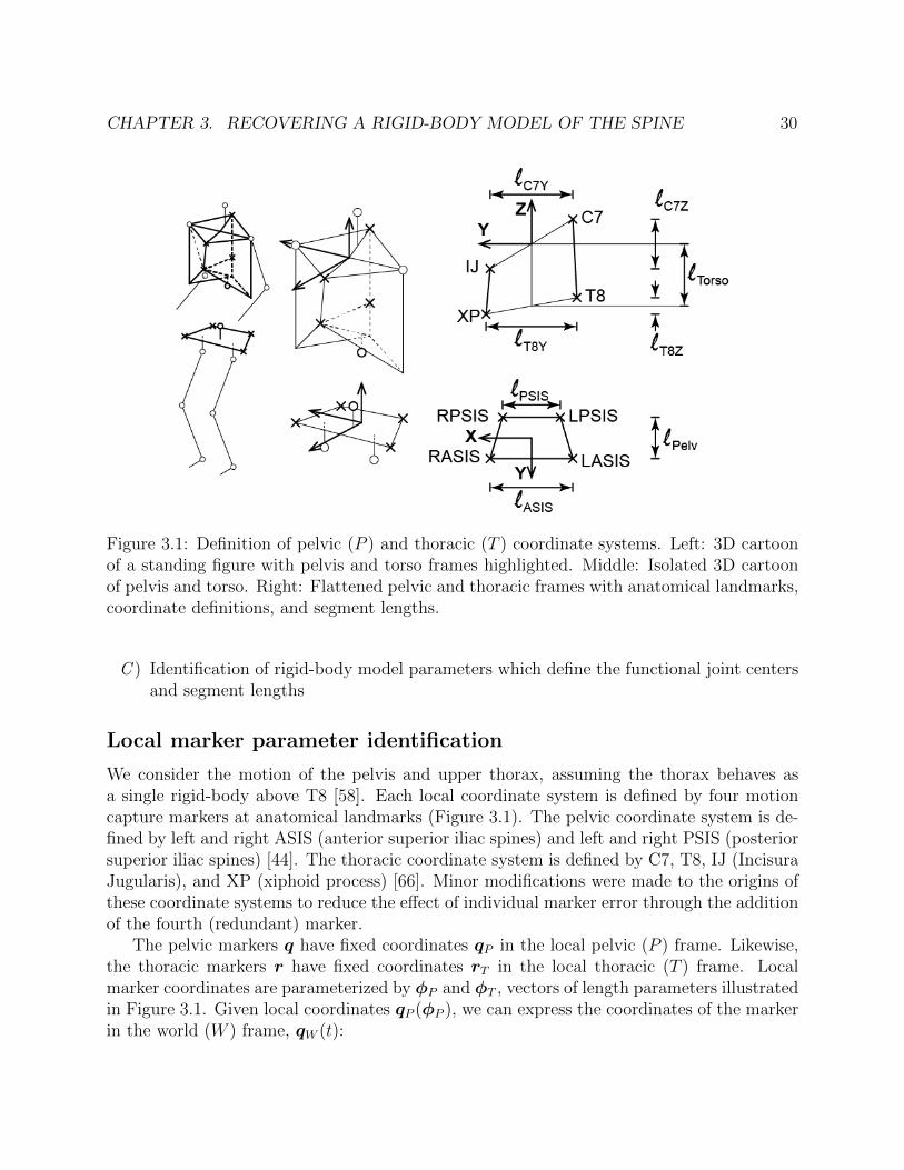
CHAPTER 3. RECOVERING A RIGID-BODY MODEL OF THE SPINE 30
Figure 3.1: Definition of pelvic (P ) and thoracic (T ) coordinate systems. Left: 3D cartoonof a standing figure with pelvis and torso frames highlighted. Middle: Isolated 3D cartoonof pelvis and torso. Right: Flattened pelvic and thoracic frames with anatomical landmarks,coordinate definitions, and segment lengths.
C ) Identification of rigid-body model parameters which define the functional joint centersand segment lengths
Local marker parameter identification
We consider the motion of the pelvis and upper thorax, assuming the thorax behaves asa single rigid-body above T8 [58]. Each local coordinate system is defined by four motioncapture markers at anatomical landmarks (Figure 3.1). The pelvic coordinate system is de-fined by left and right ASIS (anterior superior iliac spines) and left and right PSIS (posteriorsuperior iliac spines) [44]. The thoracic coordinate system is defined by C7, T8, IJ (IncisuraJugularis), and XP (xiphoid process) [66]. Minor modifications were made to the origins ofthese coordinate systems to reduce the effect of individual marker error through the additionof the fourth (redundant) marker.
The pelvic markers q have fixed coordinates qP in the local pelvic (P ) frame. Likewise,the thoracic markers r have fixed coordinates rT in the local thoracic (T ) frame. Localmarker coordinates are parameterized by φP and φT , vectors of length parameters illustratedin Figure 3.1. Given local coordinates qP (φP ), we can express the coordinates of the markerin the world (W ) frame, qW (t):

CHAPTER 3. RECOVERING A RIGID-BODY MODEL OF THE SPINE 31
qW (t) = gWP (t)qP (φP ) (3.1)
where gWP (t) is the rigid body transformation between the world and pelvic frames at timet [67]. The transformation is defined by a linear translation and rotation:
gWP (t) =
[RWP (t) pWP (t)
0 1
](3.2)
where RWP (t) is a rotation matrix, and pWP (t) are the coordinates of the center of rotationas viewed in the W frame.
The rigid-body transform can be described by the translation pWP and scaled axis ofrotation ωWP written as the vector ξ ∈ R6 where ξ = [ωWP ,pWP ]T which gives the trans-formation:
gWP (ξ) =
[eωWP pWP
0 1
]. (3.3)
The best fit local marker parameters φP and the corresponding states ξ are recoveredfrom n samples of observed marker positions in the world frame. This can be written as theoptimization:
minφP ,ξ1···ξn
n∑i=1
‖gWP (ξP (i))qP (φP )− qW (i)‖ (3.4)
where qW (i) are the observed markers in world coordinates and ξP (i) is the correspondingstate at the ith sample.
These parameters were optimized over 20 sample frames from the flexion-extension mo-tion to find the best fit local marker coordinates, using the non-linear least squares (NLS)solver in MATLAB, obtaining the marker parameters φp and local marker coordinates, qP .This process was repeated to determine the local thoracic marker positions rT . This opti-mization was performed for each subject, obtaining subject-specific pelvis and torso localmarker locations.
Transformation to the local pelvic frame
During the flexion-extension and sit to stand motions, a significant portion of the observedrotation is due to motion of the pelvis. To isolate the motion of the spine, we transform theobserved world-frame motion of the thoracic markers rW into pelvic frame coordinates rPshown in Figure 3.2. The configuration of the pelvis gWP at each frame i is recovered usingthe fixed marker model identified in Section II-A:
minξi‖gWP (ξ(i)qP )− qW )‖ . (3.5)

CHAPTER 3. RECOVERING A RIGID-BODY MODEL OF THE SPINE 32
Figure 3.2: Visualization of transformation of the motion capture markers from the Worldframe (left) into the recovered Pelvic frame (right). Data from the eight markers used in themodel recovery algorithm as well as three additional markes on the lumbar spine is shown.
This allows for the transformation of the thoracic markers from the world frame into thepelvic frame:
rP = g−1WP (ξ(i))rW (i). (3.6)
Spine model parameter identification
We consider a one-joint and two-joint rigid-body model of the spine (Figure 3.3). Themotion of the torso during FE and STS actions are assumed to be constrained to the sagittalplane, allowing the joints to be simplified to rotations about the x-axis. The one-joint modelcontains a single joint center JC between the pelvic and thoracic frames. The intermediatecoordinate frame J is defined with origin at the JC. The length parameter lJT is the distancebetween the JC and the origin of the thoracic frame. The forward kinematics of the one-jointmodel can be expressed as a series of relative rigid-body transforms:
gPT = gPJgJT
=
[Rxθ JCP
0 1
] [I3 pJT0 1
](3.7)
where Rx is the standard rotation matrix about the x-axis, θ is the angle of rotation at the
JC, JCP is the location of the JC in pelvic frame coordinates, and pJT =[0 0 lJT
]Tis
the fixed translation from the joint center to the thoracic frame.

CHAPTER 3. RECOVERING A RIGID-BODY MODEL OF THE SPINE 33
Figure 3.3: Rigid-body spine models in the pelvic (P ) coordinate system. Local coordinateframes and surface markers are labeled.
The two-joint model contains a lower joint center LJC fixed in the pelvic frame and anupper joint center UJC fixed in the thoracic frame. The intermediate coordinate frames Land U are defined with origins at the LJC and the UJC, respectively. The length parameterlLU is the distance between the LJC and the UJC. The forward kinematics of two-jointmodel can be expressed as a series of relative rigid-body transforms:
gPT = gPLgLUgUT
=
[Rxθ1 LJP
0 1
] [Rxθ2 pLU
0 1
] [I3 −UJT0 1
](3.8)
where θ1 and θ2 are the angles of rotation at the LJC and the UJC, LJP is the location of
the LJC in the P frame, UJT is the location of UJC in the T frame and pLU =[0 0 lLU
]Tis the fixed translation from the LJC to the UJC.
By grouping the joint center and length parameters for each model into a parametervector ψs (single-joint) or ψd (double-joint) the optimization problem for each model can bewritten:
minψs,θ
n∑i=1
‖gPT (ψs,θ(i))rT − rp(i)‖ (3.9)
minψd,θ1,θ2
n∑i=1
‖gPT (ψd,θ1(i),θ2(i))rT − rp(i)‖ (3.10)
where rp are the observed thoracic markers transformed to the pelvic frame using Eq. 3.6.

CHAPTER 3. RECOVERING A RIGID-BODY MODEL OF THE SPINE 34
Figure 3.4: Representative example of rigid-body models recovered from flexion-extension(top) and sit-to-stand (bottom). The models from each method are shown in the sagittalplane: functional two-joint (left), functional one-joint (center), and allometric one-joint(right). Models are plotted in the local pelvic coordinate frame with the subjects facing left.In each plot, full flexion is the left-most configuration and full-extension is the right-mostconfiguration. The ground truth thoracic frame is plotted in black.
Allometric Model
For comparison, height-based allometric relationships for the model parameters of a single-joint spine were derived using the methodology from Reed [40], the original dry pelvis datafrom Reynolds [42], and surface to spine models from Snyder [58] and Robbins [59, 68].These relationships were recomputed for the pelvic and thoracic coordinate frames specifiedin Section II-A.
3.3 Experimental Validation
Experimental Protocol
The method was evaluated on ten healthy subjects (3F/7M age: 30.9 ± 9.6 years, height:1.76 ± .12 m, mass: 67.4 ± 11.2 kg) under approval of informed consent (UCSF IRB:12-10253).

CHAPTER 3. RECOVERING A RIGID-BODY MODEL OF THE SPINE 35
Table 3.1: Parameter and state constraints for one-joint (left) and two-joint (right) models.
Variable RangeJCY [−0.05, 0.05]mJCZ [0, 0.2]mlJT [0, 0.5]mθ [−π/2, π/4] rad
Variable RangeLJCY [−0.05, 0.05]mLJCZ [0, 0.1]mUJCY [−0.05, 0.05]mUJCZ [−0.2, 0.5]mlLU [0, 0.25]m
θ1 (LJC) [−π/2, π/4] radθ2 (UJC) [−π/6, π/6] rad
An 8-camera PhaseSpace active motion capture system (480 Hz) was used to track themotion of the surface landmarks detailed in Section II-A. LED markers were placed directlyon the skin with adhesive Velcro.
The protocol consisted of three self-paced standing FE motions and three sit-to-stand andstand-to-sit actions. During FE, subjects were instructed to bend forward and backward asfar as comfortable with arms at their sides. During STS, subjects were instructed to performthe action naturally with arms at their sides.
Model Recovery and Evaluation
The methods outlined in Section II were applied to recover parameters for the one-joint andtwo-joint models. Models were separately recovered from FE and STS data, using twentyframes of data, sampled across the full range of each motion. No constraints were appliedduring step A or B of Section II. Loose constraints were applied during the optimization ofmodel parameters and joint states in step C (Table 3.1).
The recovered functional models and the allometric one-joint model were tested on FEand STS data sets, each consisting of 300 samples with training data excluded. Given fixedmodel parameters, we recover the joint angles using Equation 3.9 or 3.10. An example ofthe generated rigid-body models for a single subject is presented in Figure 3.4. Each plotdisplays the recovered spinal configuration at positions sampled across the motion. Notethat we observe a smaller range of spinal motion in STS compared to FE.
Results
From the joint state recovery process, we compute the thoracic marker residuals, the distancebetween the observed and predicted (best fit) marker locations. The mean marker residualfor each model is presented in Table 3.2. The residual plots in Figure 3.5 allow for visualinspection of the marker residuals dependence on the spine configuration (from fully extendedto fully flexed). The mean recovered subject-specific parameters for the one-joint and two-joint models are given in Table 3.3.

CHAPTER 3. RECOVERING A RIGID-BODY MODEL OF THE SPINE 36
Table 3.2: Mean thoracic marker residuals (mm) for functional and allometric models.Bolded entries indicate models trained and tested on the same motion (different data set).
Test actionModel (training action) Flexion/Extension Sit-to-StandFunctional 2-Joint (FE) 6.0 ± 3.7 7.9 ± 5.3Functional 1-Joint (FE) 9.0 ± 5.7 12.6 ± 7.3Functional 2-Joint (STS) 9.0 ± 6.4 5.3 ± 3.1Functional 1-Joint (STS) 13.6 ± 8.7 7.5 ± 4.8Allometric 1-Joint 27.2 ± 15.4 27.7 ± 14.4
Table 3.3: Mean recovered parameters for functional models. Values represent the parameteras a percentage of subject height.
Parameter Functional FE Functional STS AllometricJCY -1.4 ± 1.1 1.2 ± 1.5 1.1JCZ 4.6 ± 1.6 2.7 ± 2.7 1.84lJT 21.5 ± 1.7 23.8 ± 3.0 25.10
LJCY -1.2 ± 0.9 -0.7 ± 0.8 –LJCZ 1.6 ± 1.2 0.9 ± 1.3 –lLU 10.3 ± 2.6 8.1 ± 4.6 –UJCY -1.1 ± 0.7 -0.7 ± 1.0 –UJCZ -14.2 ± 1.5 -16.6 ± 4.6 –
3.4 Discussion
While the proposed kinematic models are representative of the observed aggregate motionof the spine, we make no claims on the relationship between the recovered joint centers andthe internal anatomy. Therefore, it is not appropriate to compare the recovered joint centersto internal imaging studies of static postures. Rather, we consider the marker residuals asan indication of the goodness-of-fit of each model.
The marker residuals of the functional methods were lower than those of the allometricmodel across both motions and all subjects (Table 3.2). The two-joint model outperformedthe one-joint model both when the models were trained and tested on the same action andwhen the models were trained and tested on a different actions. As expected, there wasa decline in performance when the functional models were trained and tested on differentmotions, though the decline was smaller for the two-joint model.
Visual analysis of the residual plots in Figure 3.5 provides additional insight into thefit of the models. The plots show the mean residual against the % of the phase (ie. theproportion of the motion completed). For a perfectly fit model, we expect to see a horizontalline, meaning the marker residuals do not vary predictable with the motion of the spine. Forthe allometric model, we observe a dependency on the phase, with greater marker residuals
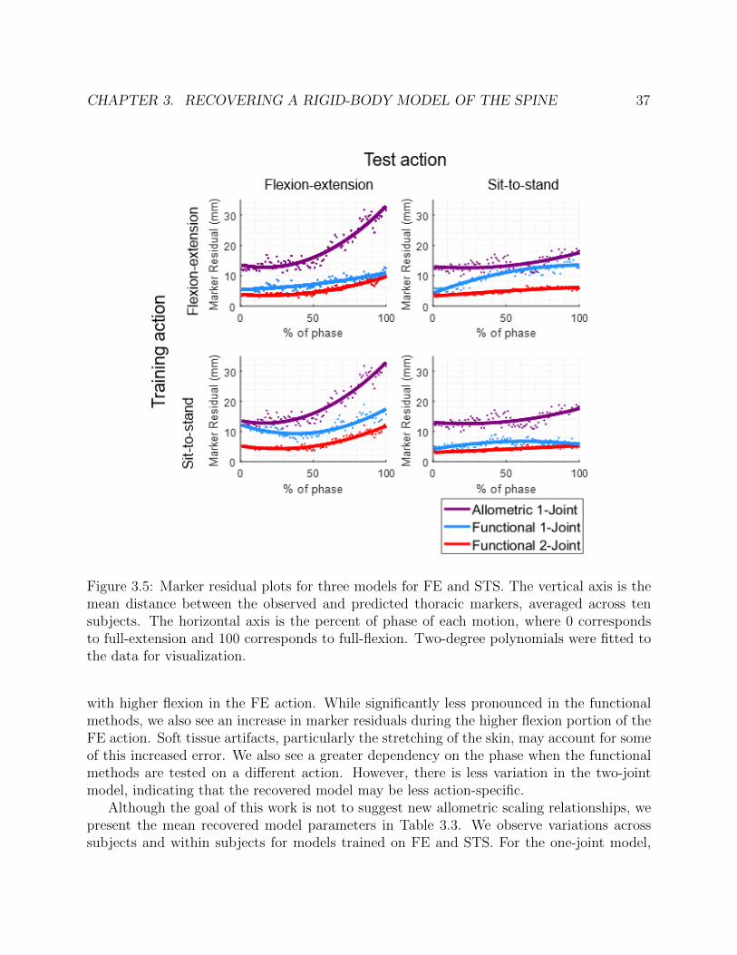
CHAPTER 3. RECOVERING A RIGID-BODY MODEL OF THE SPINE 37
Figure 3.5: Marker residual plots for three models for FE and STS. The vertical axis is themean distance between the observed and predicted thoracic markers, averaged across tensubjects. The horizontal axis is the percent of phase of each motion, where 0 correspondsto full-extension and 100 corresponds to full-flexion. Two-degree polynomials were fitted tothe data for visualization.
with higher flexion in the FE action. While significantly less pronounced in the functionalmethods, we also see an increase in marker residuals during the higher flexion portion of theFE action. Soft tissue artifacts, particularly the stretching of the skin, may account for someof this increased error. We also see a greater dependency on the phase when the functionalmethods are tested on a different action. However, there is less variation in the two-jointmodel, indicating that the recovered model may be less action-specific.
Although the goal of this work is not to suggest new allometric scaling relationships, wepresent the mean recovered model parameters in Table 3.3. We observe variations acrosssubjects and within subjects for models trained on FE and STS. For the one-joint model,

CHAPTER 3. RECOVERING A RIGID-BODY MODEL OF THE SPINE 38
there is a statistically significant (p = .009) difference between the recovered joint locationfrom FE and STS. The lower joint center in STS may be a result of less motion in the upperlumbar or thoracic vertebrae. It is necessary to train the simplified one-joint model on thetest action of interest.
3.5 Chapter Summary
The functional joint center method presented in this chapter provides a quick method forgenerating a subject-specific model of the spine for use in analysis of motion. This methoddoes not require internal imaging or rely on allometric relationships. When compared to anallometric model, the functional models result in lower marker residuals with less dependencyon the phase of the motion. This method does not provide the location of intervertebral jointcenter locations, but rather presents joint centers for a representative kinematic model ofthe aggregate motion of the spine. The formulation of the optimization limits the structureof the rigid-body model to a maximum of two joints. However, the method could be appliedto motions outside of the plane, such as lateral bending.
Future work may explore the application of this method to the analysis of spinal motionand loading in a clinical population. In contrast to allometric models or regression equations,this functional method is not based on data from a healthy population. Thus, it may havegreater applicability to a clinical population, such as subjects with spinal deformity or spinalfusion. Known fusion geometry may be incorporated into the model parameter constraintsto derive subject-specific models.

39
Chapter 4
A Passively Assistive Knee Orthotic
As described in Chapter 2, the sit-to-stand motion is an activity of daily living which requiressignificant torque generation and coordinated movement at multiple joints. It is thereforeimportant to consider the whole-body biomechanics when designing an assistive device forSTS. In this chapter, we present a passive elastic orthotic was developed which providesbilateral knee extension assistance. Initial human experiments were conducted with twosubjects under two foot-placement conditions. The human and device kinematics and dy-namics were modelled, allowing for the assessment of the biomechanical effects of the device.The assistance resulted in a decrease in the human knee torque as well as changes in whole-body biomechanics, notably an increase in the linear momentum of the upper body and adecrease in the anterior excursion of the center of mass. These results indicate that single-joint assistance at the knee has the potential to both facilitate successful STS and positivelyalter whole-body biomechanics.
4.1 Motivation and Overview
Sit-to-stand (STS) is both an activity of daily living and a common clinical test of strengthand balance. Rising from a chair requires coordinated joint motion: extension of the knees,coupled with an initial flexion and then extension of the hips [69]. The biomechanics of themotion are well-studied, including the analysis of failed STS and the identification of STSstrategies in elderly and pathological populations [70]. When compared to the momentum-transfer strategy adopted by most healthy, younger adults, elderly subjects have been foundto lean forward more, moving their center of mass over their ankles quasi-statically beforerising [71]. Conversely, individuals with low back pain rise with less hip swing and torsoinclination [72]. Although the motion can be successfully completed under these strategies,they may result in greater joint loads or a higher likelihood of STS failure. Building on thesestrategy studies, this work aims to study how passive knee assistance will affect whole-bodybiomechanics. Primarily, the goal of the device is to facilitate successful STS. However, wealso hypothesize that, in addition to reducing the required human knee torque, assistance
CHAPTER 4. A PASSIVELY ASSISTIVE KNEE ORTHOTIC 40
at the knee will alter full-body biomechanics, potentially encouraging a STS strategy witha desirable biomechanical outcome (e.g. decreased spinal loading or greater momentum).
While most lower-limb exoskeleton development has focused on gait assistance, a numberof devices have been designed specifically for STS assistance and assistance at the knee[73]. These systems are actively actuated by DC motors, series elastic actuators (SEA), orpneumatic artificial muscles, typically operating under position, force or impedance control.After a reference position or torque trajectory has been identified, a low level controller isused to provide feedback based on observed center of pressure or estimates of torque fromEMG or SEA deflection [74, 75, 76]. While these systems are able to provide a standing assist,the changes to the subject’s biomechanics and joint loads are under-studied, with analysisconstrained to predicted changes in knee torque and power. The effects of compensation andadaptation to the device are therefore neglected, with potentially beneficial factors beingomitted from the analysis. As active systems usually exhibit delays or adaptions to the user,the coupled system may behave differently to that of the individual components, so analysisof the knee joint in isolation is insufficient.
In addition, these powered systems require complex controllers and are limited by cost,weight, and energy consumption. In contrast, passive or passive/active systems utilize ad-justable energy storage mechanisms such as electrostatically clutched elastics or pneumaticsto adjust the dynamic response of the human-device system, providing assistance for upperor lower limbs [77, 78, 79]. Notably, a quasi-passive knee exoskeleton has been developed toprovide various levels of assistive stiffness in parallel with the knee during gait with analy-sis of the biomechanical effects at the ankle, knee, and hip joints [80], [81]. Tuned passivedevices have also been shown to provide super-human ability in the form of decreased VO2
consumption during gait [82]. As a measure of endurance, VO2 is not an appropriate met-ric for an activity such as STS which is not aerobically limited. This we therefore presentchanges in the observed biomechanics, specifically the joint torque, body momentum, andcenter of mass trajectory which may correspond to limitations in strength, coordination, orspeed.
Contributions
We introduce a passive knee orthotic designed to provide bilateral assistance in knee exten-sion during STS. The system utilizes an elastic element to generate an assistive torque witha fraction of the mass required by an equivalent active system. The device and resultingmotion are assessed on two healthy subjects performing STS under two initial foot placementconditions. Initial analysis demonstrates the feasibility of the device to induce changes inknee and whole-body biomechanics.

CHAPTER 4. A PASSIVELY ASSISTIVE KNEE ORTHOTIC 41
Figure 4.1: Assistive knee orthotic. Left: Device worn by a subject on their left knee (rightknee hidden). Center: Schematic of knee assistive system. Elastic band, pulley, and braceas indicated. Right: Characterization curve for the knee orthotic. Flexion and extensiondirections are as shown.
4.2 Methods
Mechanism Design
A knee orthosis (Figure 4.1) was developed to provide passive assistance at the knee duringthe STS motion. The angular trajectory of the knee joint during a typical STS consists ofexclusively knee extension, whereas the ankle and hip exhibit a combination of flexion andextension. This pure knee extension facilitates the application of a simple passive componentwithout a clutch or other complex mechanism or control scheme. Assistance at the knee isgenerated by the linear extension of an elastic component which wraps around the knee toproduce a torque. Exerting no torque at a full standing position, the device stores energy asthe knee is flexed during sitting. This energy is then released during standing, providing anassistive torque in knee extension.
The device was developed by augmenting a commercially available knee brace (DonJoyLegend SE-4) which is used to provide stability following knee injury. The brace was selectedfor its recommended use during sports activities, allowing for a full range of motion. A 78mm diameter, 15 mm thick Delrin puck was added onto the knee center of the brace to actas a fixed pulley. Two guides were fabricated out of aluminium and fixed to either side ofthe pulley.
The elastic band was constructed from a 5/8” outer diameter, 1/8” inner diameter rub-ber tube (Primeline Industries, Ohio) which was cut into a 1” length. Two stainless steelwishbone inserts were used to attach 2.5 mm Spectra line to each end. The band was securedonto the wishbone insert using a constrictor knot made from 1 mm braided Kevlar. Theband was secured onto the brace so that there was slight pre-tension in the line when fully

CHAPTER 4. A PASSIVELY ASSISTIVE KNEE ORTHOTIC 42
extended. An R-clip was used to constrain the Spectra to lie between the pulley guides. Thetotal mass of each orthotic was 0.81 ± 0.01 kg.
It is important to note that the device was designed to enable the study of biomechanicaleffect of assistance during STS, rather than to be worn in daily assistance in its currentform. As the mechanism of assistance is designed with consideration for STS, the devicewould likely inhibit knee motion during gait or other activities.
Device Characterization
Bench-top characterization of the device torque-angle relationship was performed immedi-ately prior to and after each human experiment. With one side of the brace clamped, thecontact force at the opposing side was measured using a 6-axis force/torque sensor (ATIMini-45, ATI Industrial Automation), recording the force measurements at 1000 Hz as thedevice was manually moved through its full range of motion five times at a gentle pace.Motion capture data of the brace was simultaneously collected to measure the knee flexionangle. The resulting torque-angle curve is shown in Figure 4.1. While hysteresis was ob-served between flexion and extension, the device was found to provide a repeatable torqueresponse. The maximum assistance provided by the device was measured to be 12 Nm at aknee flexion of 1.5 rad with an approximately linear relationship. The amount of assistancecan be adjusted by changing the length or material properties of the band. During testing,a brace is worn on both the left and right legs, providing total assistance equal to twice thecharacterized value.
Human-Device Model
To assess the motion and analyze the contribution of the knee assistance, it is necessaryto model the kinematics and dynamics of the STS motion. A sagittal-plane rigid-bodymodel is used to perform planar inverse kinematic and inverse dynamic analysis. The modelconsists of revolute joints at the ankle, knee, hip, and lower-lumbar (L5-S1). Length andbody segment center of mass parameters were allometrically-scaled by the subject’s heightand mass [2]. The recovered joint angles can be converted to velocities and accelerationswhich are propagated through each segment. The wrench in the local body-frame can thenbe computed to provide estimates of joint torques and powers [83]. The estimated resultantknee torque τr obtained through this method is then decomposed into the device τd andhuman τh components based on the prior device characterization:
τh = τr − τd (4.1)
4.3 Experiment
Motion capture and force data were collected to study the effect of bilateral knee assistanceon full-body biomechanics during STS. This preliminary data was collected from two healthy

CHAPTER 4. A PASSIVELY ASSISTIVE KNEE ORTHOTIC 43
young-adult subjects (S01: male, age 30, 1.78 m height, 65 kg weight, and S02: female, age26, 1.55 m height, 56 kg weight) under informed consent (UCB IRB protocol 2018-04-10940).
Kinematic data was collected from an 8-camera motion capture system (PhaseSpaceImpulse X2, PhaseSpace Inc., San Leandro, CA, USA) at 480 Hz. Markers were placeddirectly on the skin using adhesive Velcro according to an augmented Plug-In Gait protocol[43], allowing for recovery of the sagittal plane human model. Additional markers wereplaced on triads mounted on the knee brace. Ground reaction forces were collected with a6-axis force platform (AMTI, Massachusetts). Additional forces were collected from a 6-axisforce/torque sensor (ATI Industrial Automation) mounted inside of a custom chair.
The STS motion was performed under two initial kinematic configurations: natural footplacement and anterior foot placement. The natural position was self-selected by each subjectas a comfortable standing position. The anterior foot position was selected at a knee flexionangle of approximately 1.2 rad. This position was chosen to make the STS motion morebiomechanically challenging.
STS motions at each foot position were tested under two device conditions, unassistedand assisted, resulting in four total testing conditions. In the unassisted mode, the subjectwore the brace with the band disengaged.
For each of the four testing modes, the subject completed three trials consisting of sevenSTS motions. The subject began each trial in a seated position and was instructed to foldtheir arms across their chest. The subject was otherwise not coached on how to stand. Ametronome at 30 beats per minute was used to indicate when to stand and sit. This allowedfor a period of quiet sitting and quiet standing between each sitting or standing action.
Joint positions were estimated from motion capture data using an allometrically-scaledmodel [2]. The resulting joint angles were then repeatedly filtered and numerically differ-entiated (Butterworth, 2nd order, 6 Hz) to obtain the corresponding angular velocity andacceleration trajectories.
4.4 Biomechanical Effects of Assistance
This section introduces key biomechanical features for the assisted and unassisted standingactions. Analysis is performed at the knee specifically (Section 4.4) as well the whole-bodymotion (Section 4.4).
Knee Torque
The torque response curves for the knee are shown in Figure 4.2 with knee extension cor-responding to a negative torque. The knee torque is evaluated from the moment of seatoff (defined as the point at which the vertical force in the chair is less than 20 N) to quietstanding (defined by zero torso velocity). For the assisted mode, the resultant torque (red) isdecomposed into the predicted device torque (black) and human torque (green). It is shownalongside the human torque from the unassisted motion (blue).

CHAPTER 4. A PASSIVELY ASSISTIVE KNEE ORTHOTIC 44
Figure 4.2: Knee torque during sit-to-stand as a function of time (left) and knee angle (right).Each plot has three lines for the assistive mode: the resultant torque from the human anddevice (red), the device torque (black), and the remaining human torque (green). Addition-ally, the human torque in the unassistive mode is plotted in blue. The trace represents themean trajectory across all trials with the standard deviation shown as a shaded region of thesame colour. The plots are shown for each subject and separated by the natural foot (toprow) and anterior foot placement (bottom row) conditions.
Under assistance, there is an expected decrease in the human torque required. In thetorque-angle curves, we observe that the human torque during the assisted mode initiallyaligns with the unassisted human torque. At a knee angle of approximately -1 radians, theassisted human torque decreases so that the resultant torque matches the unassisted humantorque. This suggests that the subjects may exploit the assistance partway through theaction. This pattern is consistent across trials, suggesting that subjects are not adapting tothe assistance over trials. An exception is seen in the anterior foot placement condition forS02, in which the human provides an abating knee torque in the second half of the motion.This observed torque in the knee flexion direction appears to compensate for greater trunkmomentum. The whole-body biomechanical analysis (4.4) indicates that the subject changedtheir standing strategy under these conditions.

CHAPTER 4. A PASSIVELY ASSISTIVE KNEE ORTHOTIC 45
Figure 4.3: Trajectory of the center of mass (COM) of the head-arms-trunk segment duringSTS with natural foot placement (top) and anterior foot placement (bottom). Trajectoriesare normalized by subject height with the average taken across all trials for each subject.Blue lines denote assisted trajectory and Red lines denote unassisted trajectory.
Whole-body Biomechanics
Center of Mass
For both foot configurations, the assistance at the knee resulted in a steeper vertical rise ofthe head-arms-trunk (HAT) body segment. This can be observed in the trajectory of theHAT center of mass (COM) shown in Figure 4.3. This smaller anterior excursion of theCOM corresponds to less trunk inclination during the motion.
Torso Momenta
The torso momenta p are computed from the body velocities of the torso and the torsoinertia tensor Itorso:
p = ItorsoVbtorso (4.2)
Figure 4.4 shows the vertical component of the linear momentum of the HAT segment.Under all conditions, the peak vertical linear momentum increases with the assistance atthe knee. With normal foot placement, the momentum consists of a single peak, suggestinga single momentum transfer action, moving the COM forward and up vertically. This isseen in the assisted and unassisted modes for both subjects. For the anterior foot placementcondition, the unassisted mode appears to consist of two separate sections. This may indicatea leaning strategy where the first peak corresponds to the initial movement of the torso,

CHAPTER 4. A PASSIVELY ASSISTIVE KNEE ORTHOTIC 46
Figure 4.4: Vertical linear momentum of the head-arms-trunk segment. Unassisted motionis shown in red dashed line with assisted motion in blue solid line. The values are normalizedby subject height and mass and shown for S01 (left) and S02 (right) under the natural footplacement (top row) and anterior foot placement (bottom row). In each plot, the mean over21 motions is shown with the standard deviation in shaded bounds.
CHAPTER 4. A PASSIVELY ASSISTIVE KNEE ORTHOTIC 47
before there is a second separate rise. For S02 in the anterior foot condition, a transitionis seen from a lean strategy to a momentum transfer strategy in the assisted mode. Thischange in strategy is not seen in S01.
The passive orthotic was able to provide assistance which resulted in lower knee loadingand changes in whole-body kinematics and dynamics. This initial biomechanical analysissupports the hypothesis that passive extension assistance at the knee has the potential to af-fect full-body biomechanics during STS. The increase in upper body vertical momentum wasobserved for both subjects under all assisted testing conditions. This change in momentum,alongside the corresponding decrease in the anterior excursion of the COM, are promisingfor improved motions as low vertical momentum was found to be an indicator of failed STS[70].
4.5 Chapter Summary
In this chapter, we present a new device for assistance in knee extension during STS. Aug-menting an existing knee orthotic, the device incorporates a simple elastic elemant to providepassive assistance. Our results support the hypothesis that assistance at a single joint canaffect whole-body motion. Additionally, our bio-mechanical analysis highlight the variedeffect even simple systems can have on whole-body biomechanics and that, even for simplesystems, people may respond differently. While providing knee extension assistance duringsit-to-stand decreased the average human knee torque for both standing conditions, the effecton the low-back and hips varied. By studying the full-body biomechanical effects of assistivesystems, simple devices can be developed to encourage specific motions.
Limitations
Only two healthy subjects were tested in this study over a short time horizon, makinggeneralization on the effect of this system to other subjects, particularly patient groupsunclear. Similarly, analysis only occurred in the sagittal plane with the effect of the motionof the arms neglected. The validity of these assumptions needs to be tested as part of awider study.
Future Work
While this chapter introduces a method for altering whole-body motion, the relationshipbetween the assistance and the resulting motions is not known. A more detailed studythat builds on a parameterized model of STS, and a variable stiffness actuator would allowfor rapid assessment of the effect of different extension profiles on whole-body standing andbalance. A better understanding of the underlying mechanisms for whole-body biomechanicschanges would be an electromyography(EMG) study, focusing on the differences in muscleactivation in the knee flexors, lower back, and abdominal core muscles. Finally, in order

CHAPTER 4. A PASSIVELY ASSISTIVE KNEE ORTHOTIC 48
to translate this method to provide daily assistance, future work must include mechanismdevelopment to allow for free or assisted motion during gait.

49
Chapter 5
An Affordable Device for RoboticTherapy
Since its inception in the 1980s, the field of rehabilitation robotics has seen significant ad-vances in the development of complex mechanisms and controllers. These robotic deviceshave the potential to facilitate precise, high-intensity, and adaptable rehabilitative taskswhile tracking quantitative measures of subject ability. Studies of robot-assisted therapy,however, have only demonstrated modest benefits over traditional therapy, and we haveyet to see a widespread adoption of robotic therapy as the standard of care for in-clinicor at-home therapy. While several factors inhibit the adoption of rehabilitation robotics,an undeniable barrier results from high device cost and complexity. This inaccessibilityfurther contributes to a limited understanding of models of recovery and optimal roboticrehabilitation protocols.
We aim to address the limitation of cost and complexity through the introduction of anaffordable planar manipulanda for upper limb assessment and therapy. With a total partcost of less than $800, the device utilizes inexpensive and off-the-shelf components to provideactive assistance and resistance. It is capable of guiding the arm through trajectories, fol-lowing the subject’s intended motion through force-based admittance control, and imposingassistive or resistive force-fields while tracking the position and force exerted by the subject.In this chapter, we present our design objectives and outline the mechanical, electrical, andsoftware systems. We validate the device performance and present a new method for deter-mining the human arm 3D upper-limb inverse kinematics with the device. Finally, we showinitial data from human subjects interacting with the developed system.

CHAPTER 5. AN AFFORDABLE DEVICE FOR ROBOTIC THERAPY 50
Figure 5.1: Examples of upper-limb robotic rehabilitation devices. A: In-Motion Arm, thecommercial version of the MIT-MANUS [84], B: ARMin 4 [85], C: H-Man [86], D: NeRoBot[87].
5.1 Overview of Upper Limb Rehabilitation Robotics
During robot-assisted therapy, a robotic device provides continuous physical interaction witha subject to complete a rehabilitation protocol. This therapy can be incorporated into reha-bilitation for subjects with upper limb impairment due to neurological injury such as strokeor spinal cord injury [88]. Stroke is a leading cause of disability in the United States, withmany patients experiencing impairment of the upper limb [89]. This motor impairmentcan manifest in several ways including weakness, spasticity, loss of coordination, and ab-normal muscle synergies. The presence of impairments of the upper-limb and hand inhibitthe ability to perform activities of daily living and live independently [90]. The incorpora-tion of robotic technology into rehabilitation therapy is desirable because of the ability toprovide high-intensity protocols targeted protocols while recording quantitative measures ofperformance.
There exists an array of robotic therapy devices targeted at the lower limbs, upper limbs,
CHAPTER 5. AN AFFORDABLE DEVICE FOR ROBOTIC THERAPY 51
and hands. We focus on devices for the upper-limb with a few examples of devices shown inFigure 5.1. When describing a robotic therapy device, we can make distinctions based on themechanism and control architecture. These design choices impact how the subject interactswith the device. Upper-limb rehabilitation robots can be classified as an exoskeleton orend-effector device based on the mechanical structure. Exoskeleton devices have a structurewhich allows for the control of individual human joints, with the device structure mimickingthe anatomical structure of the human. An example is the ARMin device shown in Figure5.1 B [85]. In contrast, end-effector devices only connect to the subject at the human hand,with the human elbow and shoulder joints moving to achieve the end-effector pose. Thissimplification does not allow for individual joint motion, but facilitates the implementation ofless-complex control schemes and less individual mechanical tuning of the device. Examplesinclude the MIT-MANUS, H-Man, and NeRoRobot shown in Figure 5.1 [84, 86, 87].
Robotic devices can be used to implement a variety of control modalities for robotictherapy. In describing a controller as assistive, we make a distinction based on how thesubjects interacts with the robotic device. In comparison to are purely passive controller, inwhich the robot completes the motion without input from the subject, and a purely activecontroller, in which the robot only measures the motion with no impact on the subject’smotion, an assistive controller requires the motion to be generated by the subject withvarying forms robotic assistance to complete the task or improve performance [90]. Examplesof assistive controllers include force-based impedance controller [84, 85], virtual walls movingtangent or normal to a trajectory [84, 91], or trigger-based assistance in which a thresholdof subject movement initiates the motion [92].
While there have been numerous studies on the design and control of robotic devices,an understanding of the clinical effectiveness of different robotic controllers is limited [93].This is due in part to a limited number of studies and study size. In addition to the highcost of robotic devices, most are used only in specialized therapeutic institutes and requireoperational supervision by expert personnel [94, 95]. To further understand the efficacy ofrobotic therapy and develop predictive models for optimal rehabilitation protocols, thereremains a need for simple, inexpensive, robotic devices.
5.2 Device Design
In this section we describe our robotic therapy device shown in Figure 5.2.
Design Objectives
With the aim of developing an affordable manipulanda for robot-assisted therapy and as-sessment, we first establish a set of design objectives:
1. Produce active motion to move the arm along arbitrary trajectories in the transverse(horizontal) plane
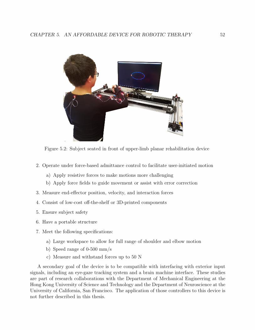
CHAPTER 5. AN AFFORDABLE DEVICE FOR ROBOTIC THERAPY 52
Figure 5.2: Subject seated in front of upper-limb planar rehabilitation device
2. Operate under force-based admittance control to facilitate user-initiated motion
a) Apply resistive forces to make motions more challenging
b) Apply force fields to guide movement or assist with error correction
3. Measure end-effector position, velocity, and interaction forces
4. Consist of low-cost off-the-shelf or 3D-printed components
5. Ensure subject safety
6. Have a portable structure
7. Meet the following specifications:
a) Large workspace to allow for full range of shoulder and elbow motion
b) Speed range of 0-500 mm/s
c) Measure and withstand forces up to 50 N
A secondary goal of the device is to be compatible with interfacing with exterior inputsignals, including an eye-gaze tracking system and a brain machine interface. These studiesare part of research collaborations with the Department of Mechanical Engineering at theHong Kong University of Science and Technology and the Department of Neuroscience at theUniversity of California, San Francisco. The application of those controllers to this device isnot further described in this thesis.

CHAPTER 5. AN AFFORDABLE DEVICE FOR ROBOTIC THERAPY 53
Figure 5.3: Diagram of the mechanical structure of the robot
Mechanical Design
The mechanical structure of our device is shown in Figure 5.3. The system consists of abelt-driven transmission which enables 2D motion in the horizontal plane. This H-shapeddifferential drive is heavily inspired by the design of H-man [86], a planar manipulanda forhaptic interaction. The differential transmission allows for a single belt to move a centralplatform, while minimizing the inertia of additional transmission elements such as motorsby keeping them fixed. In contrast to linkage-based systems, this mechanical architectureresults in simplified kinematics and high isotrophy. While we utilize the general mechanismstructure of H-man, our mechanical design and control implementation differs to achieve theaforementioned design criteria. Notably, we alter the mechanism to have a large workspace,with a new design for the center carriage and human-robot connection at the wrist. Theuse inexpensive actuation and force sensing systems require changes throughout the systemarchitecture which are detailed below.
The transmission controls the motion of the end-effector, a platform onto which thesubject’s forearm is mounted at the wrist. This wrist platform can translate in the x-directionalong two rails via linear bearings mounted in the platform. These rails connect on eitherside to a carriage assembly. Each carriage assembly is mounted on a rail via another pairlinear bearings, allowing for translation of the wrist platform and carriages in the y-direction.The motion of the wrist platform is guided by the transmission belt which is is mounted to
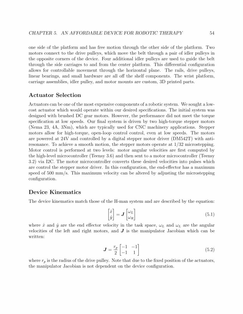
CHAPTER 5. AN AFFORDABLE DEVICE FOR ROBOTIC THERAPY 54
one side of the platform and has free motion through the other side of the platform. Twomotors connect to the drive pulleys, which move the belt through a pair of idler pulleys inthe opposite corners of the device. Four additional idler pulleys are used to guide the beltthrough the side carriages to and from the center platform. This differential configurationallows for controllable movement through the horizontal plane. The rails, drive pulleys,linear bearings, and small hardware are all off the shelf components. The wrist platform,carriage assemblies, idler pulley, and motor mounts are custom, 3D printed parts.
Actuator Selection
Actuators can be one of the most expensive components of a robotic system. We sought a low-cost actuator which would operate within our desired specifications. The initial system wasdesigned with brushed DC gear motors. However, the performance did not meet the torquespecification at low speeds. Our final system is driven by two high-torque stepper motors(Nema 23, 4A, 3Nm), which are typically used for CNC machinery applications. Steppermotors allow for high-torque, open-loop control control, even at low speeds. The motorsare powered at 24V and controlled by a digital stepper motor driver (DM542T) with anti-resonance. To achieve a smooth motion, the stepper motors operate at 1/32 microstepping.Motor control is performed at two levels: motor angular velocities are first computed bythe high-level microcontroller (Teensy 3.6) and then sent to a motor microcontroller (Teensy3.2) via I2C. The motor microcontroller converts these desired velocities into pulses whichare control the stepper motor driver. In this configuration, the end-effector has a maximumspeed of 500 mm/s. This maximum velocity can be altered by adjusting the microsteppingconfiguration.
Device Kinematics
The device kinematics match those of the H-man system and are described by the equation:[xy
]= J
[ωL
ωR
](5.1)
where x and y are the end effector velocity in the task space, ωL and ωL are the angularvelocities of the left and right motors, and J is the manipulator Jacobian which can bewritten:
J =rp2
[−1 −1−1 1
](5.2)
where rp is the radius of the drive pulley. Note that due to the fixed position of the actuators,the manipulator Jacobian is not dependent on the device configuration.
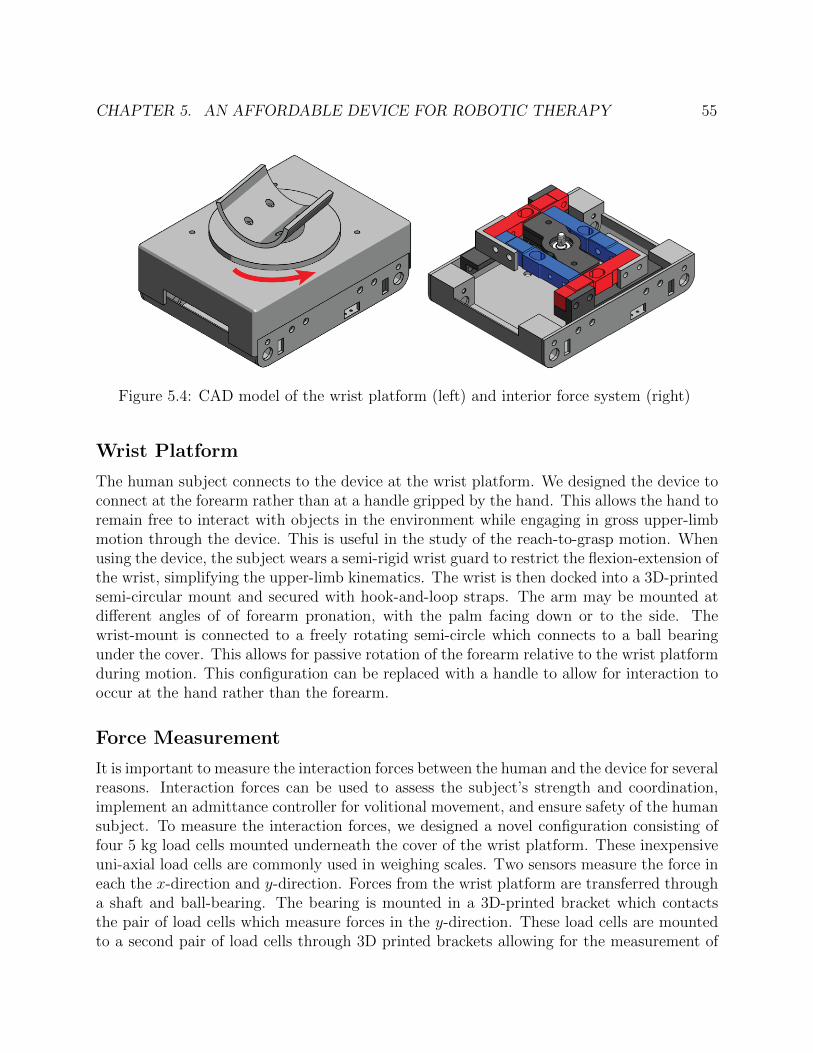
CHAPTER 5. AN AFFORDABLE DEVICE FOR ROBOTIC THERAPY 55
Figure 5.4: CAD model of the wrist platform (left) and interior force system (right)
Wrist Platform
The human subject connects to the device at the wrist platform. We designed the device toconnect at the forearm rather than at a handle gripped by the hand. This allows the hand toremain free to interact with objects in the environment while engaging in gross upper-limbmotion through the device. This is useful in the study of the reach-to-grasp motion. Whenusing the device, the subject wears a semi-rigid wrist guard to restrict the flexion-extension ofthe wrist, simplifying the upper-limb kinematics. The wrist is then docked into a 3D-printedsemi-circular mount and secured with hook-and-loop straps. The arm may be mounted atdifferent angles of of forearm pronation, with the palm facing down or to the side. Thewrist-mount is connected to a freely rotating semi-circle which connects to a ball bearingunder the cover. This allows for passive rotation of the forearm relative to the wrist platformduring motion. This configuration can be replaced with a handle to allow for interaction tooccur at the hand rather than the forearm.
Force Measurement
It is important to measure the interaction forces between the human and the device for severalreasons. Interaction forces can be used to assess the subject’s strength and coordination,implement an admittance controller for volitional movement, and ensure safety of the humansubject. To measure the interaction forces, we designed a novel configuration consisting offour 5 kg load cells mounted underneath the cover of the wrist platform. These inexpensiveuni-axial load cells are commonly used in weighing scales. Two sensors measure the force ineach the x-direction and y-direction. Forces from the wrist platform are transferred througha shaft and ball-bearing. The bearing is mounted in a 3D-printed bracket which contactsthe pair of load cells which measure forces in the y-direction. These load cells are mountedto a second pair of load cells through 3D printed brackets allowing for the measurement of

CHAPTER 5. AN AFFORDABLE DEVICE FOR ROBOTIC THERAPY 56
Figure 5.5: Top-down view of the force system
force in the x-direction. The force at the contact point can then be resolved as the sum ofall forces:
Fx = F1x + F2x (5.3)
Fy = F1y + F2y (5.4)
The force subsystem electronics are mounted within the wrist platform. The load cellvoltage is measured by an analog-to-digital converter with a programmable gain amplifier(ADS115). These measurements are then sent to the force microcontroller (Teensy 3.2) viaI2C. The force subsystem is shown in Figure 5.8. The load cell configuration is capable ofmeasuring a maximum 10 kg, or 98.06 N, in any direction, with a resolution of .074 N. TheADC chips were selected to maximize the loop speed with a tradeoff in decreased resolution.The maximum load capacity exceeds the 50 N design objective. While a limitation of thesystem is the inability to measure out of plane forces and torques, these are not necessarygiven the mechanical design of the system. The device mechanically supports the wrist alongthe z-axis. The wrist attachment is designed to minimize torques about the x- and y- axes.Finally, given the two-link upper limb system enforced by bracing the wrist, it is not possiblefor the subject to generate a torque about the z-axis.
Electronics Design
The electronic system architecture (shown in Figure 5.6) consists of a main microcontrollerwhich connects to a motor subsystem (Figure 5.7), a force subsystem (Figure 5.8), and aPC user interface. The main microcontroller is a Teensy 3.6 which features a 32 bit ARMCortex-M4 processor. This microcontroller operates at a 330 Hz loop frequency. The force

CHAPTER 5. AN AFFORDABLE DEVICE FOR ROBOTIC THERAPY 57
Figure 5.6: Electronic system architecture
and motor subsystems both use a Teensy 3.2 microcontroller, with connections via I2C.Separate microcontrollers were used for these subsystems to maximize the main control loopfrequency. The graphical user interface is run in Python and used to set the controller andexperimental parameters and log robot state data. It includes a real time visualization ofthe robot state, including end-effector position and force, as well as an interface to save thedata files. The user interface includes a subject-facing display on a separate monitor whichcan display the desired task and the real time position of the end-effector. The position ofthe wrist platform is measured by absolute magnetic encoders (US Digital MA3) mountedto each of the drive motor shafts.
Safety Considerations
When designing any system that interacts with a human, it is essential to implement a num-ber of safeguards to mitigate the risk of injury or discomfort to the subject. Workspacelimitations prevent the device from moving outside of a subjects comfortable reachableworkspace. These are implemented in software as virtual walls which can be customizedto each subject alongside limitations on maximum velocity and force. The device powerruns in series with two emergency stop buttons which are held by the subject and researcherduring experiments. Hitting the button will cut power to the motors. Additionally, there isa software emergency stop in the graphical user interface which will set all motor velocitiesto zero. Mechanical hardware limits are enforced through physical limit switches which aretriggered at the edges of the device workspace. These limit switches are also utilized duringthe position calibration procedure.

CHAPTER 5. AN AFFORDABLE DEVICE FOR ROBOTIC THERAPY 58
Figure 5.7: Diagram of the motor electronics subsystem
Figure 5.8: Diagram of the force measurement electronics subsystem
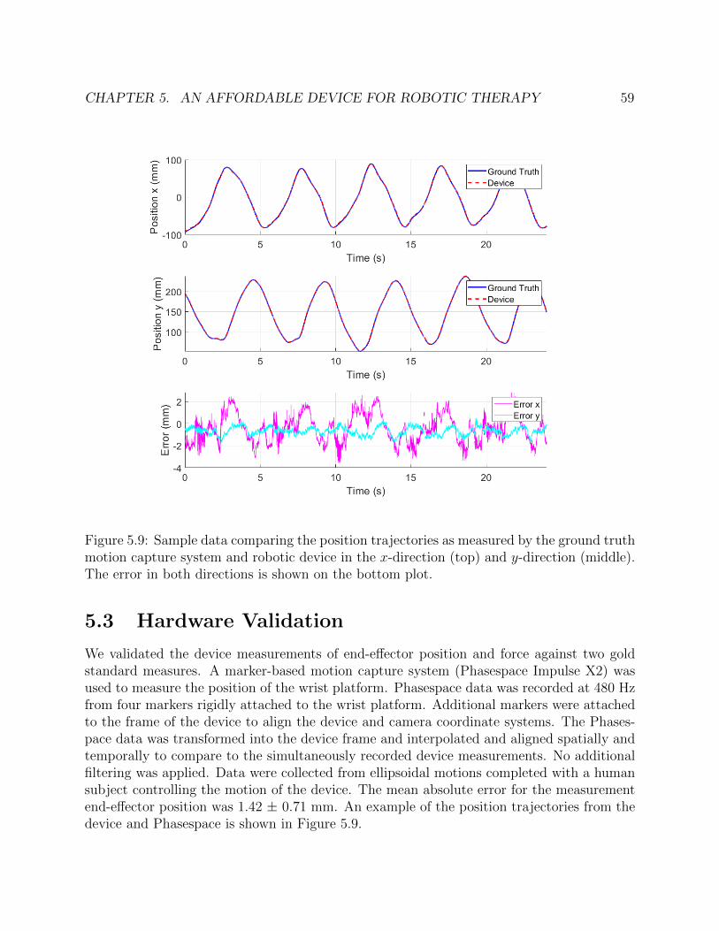
CHAPTER 5. AN AFFORDABLE DEVICE FOR ROBOTIC THERAPY 59
Figure 5.9: Sample data comparing the position trajectories as measured by the ground truthmotion capture system and robotic device in the x-direction (top) and y-direction (middle).The error in both directions is shown on the bottom plot.
5.3 Hardware Validation
We validated the device measurements of end-effector position and force against two goldstandard measures. A marker-based motion capture system (Phasespace Impulse X2) wasused to measure the position of the wrist platform. Phasespace data was recorded at 480 Hzfrom four markers rigidly attached to the wrist platform. Additional markers were attachedto the frame of the device to align the device and camera coordinate systems. The Phases-pace data was transformed into the device frame and interpolated and aligned spatially andtemporally to compare to the simultaneously recorded device measurements. No additionalfiltering was applied. Data were collected from ellipsoidal motions completed with a humansubject controlling the motion of the device. The mean absolute error for the measurementend-effector position was 1.42 ± 0.71 mm. An example of the position trajectories from thedevice and Phasespace is shown in Figure 5.9.

CHAPTER 5. AN AFFORDABLE DEVICE FOR ROBOTIC THERAPY 60
Figure 5.10: Sample data comparing the force trajectories as measured by the ground truthforce/torque sensor and robotic device in the x-direction (top) and y-direction (middle). Theerror in both directions is shown on the bottom plot.
The device measurement of the force was compared against a 6-axis force/torque sensor(ATI Automation). Note that the device load cell configuration does not measure forcesoutside of the horizontal plane. The out of plane forces and torques, therefore, are not con-sidered. To compare the forces, a custom mount was designed to attach the ATI force/torquesensor directly above the device load cell in place of the wrist mount. A handle was attachedto the opposing side of the force/torque sensor. Forces were manually applied to the handleby the investigator. Forces were applied in each of the 8 cardinal directions. An exampleof the force measurements is shown in Figure 5.10. The mean absolute error for the forcein the x-direction was 0.3 ± 0.2 N and for the y-direction was 0.53 ± 0.31 N. These resultsindicate that the position and force measurements are consistent with those measured byground truth systems.
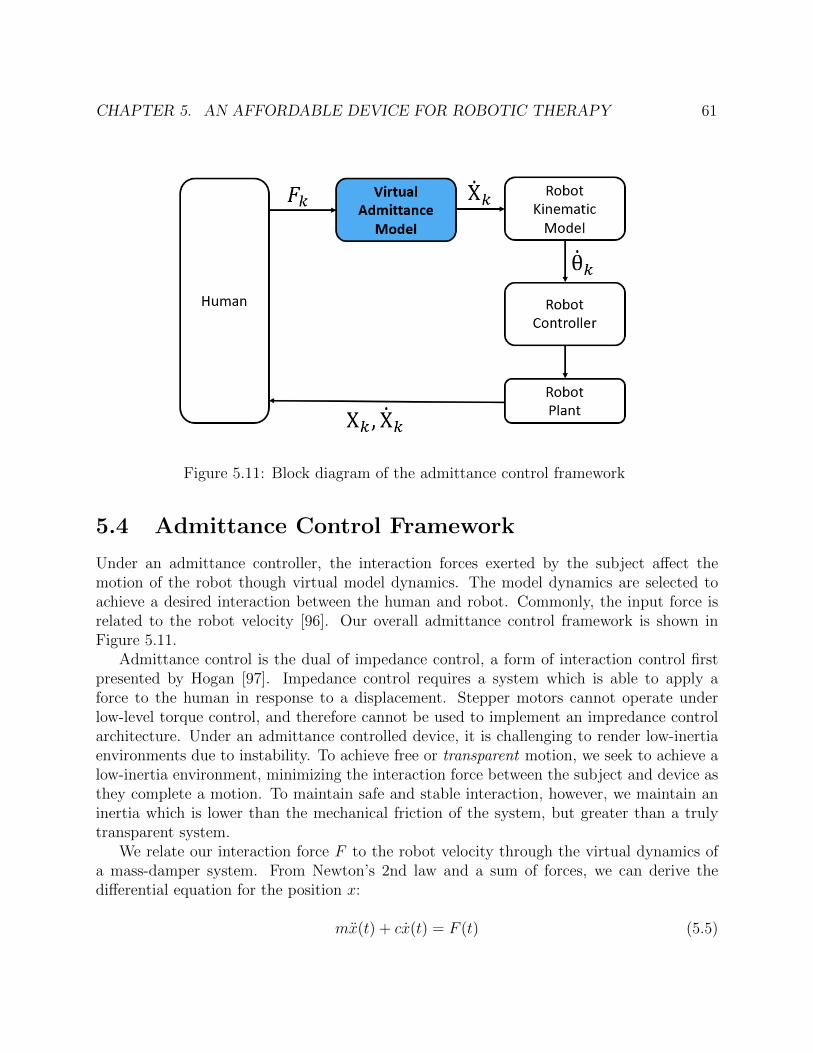
CHAPTER 5. AN AFFORDABLE DEVICE FOR ROBOTIC THERAPY 61
Figure 5.11: Block diagram of the admittance control framework
5.4 Admittance Control Framework
Under an admittance controller, the interaction forces exerted by the subject affect themotion of the robot though virtual model dynamics. The model dynamics are selected toachieve a desired interaction between the human and robot. Commonly, the input force isrelated to the robot velocity [96]. Our overall admittance control framework is shown inFigure 5.11.
Admittance control is the dual of impedance control, a form of interaction control firstpresented by Hogan [97]. Impedance control requires a system which is able to apply aforce to the human in response to a displacement. Stepper motors cannot operate underlow-level torque control, and therefore cannot be used to implement an impredance controlarchitecture. Under an admittance controlled device, it is challenging to render low-inertiaenvironments due to instability. To achieve free or transparent motion, we seek to achieve alow-inertia environment, minimizing the interaction force between the subject and device asthey complete a motion. To maintain safe and stable interaction, however, we maintain aninertia which is lower than the mechanical friction of the system, but greater than a trulytransparent system.
We relate our interaction force F to the robot velocity through the virtual dynamics ofa mass-damper system. From Newton’s 2nd law and a sum of forces, we can derive thedifferential equation for the position x:
mx(t) + cx(t) = F (t) (5.5)
CHAPTER 5. AN AFFORDABLE DEVICE FOR ROBOTIC THERAPY 62
where m is the mass and c is the damping coefficient. For implementation, we derive thediscrete dynamics via backwards Euler discretization:
xk =4tmFk +
(1− c4t
m
)Xk−1 (5.6)
where 4t is the control loop time step. We define controller parameters αm and αv tosimplify the discussion of mass and viscosity:
αm =4tm
(5.7)
αv =
(1− c4t
m
)(5.8)
Adjusting the mass and viscosity parameters affects the virtual dynamics of the human-robot-interactions. Increasing the mass parameter results in a decrease in the virtual massmass. This will result in a more responsive system, requiring less force to achieve a given ve-locity. Increasing the viscosity parameter results in greater velocity carryover of the previousvelocity state.
Upper Limb Inverse Kinematics
While the device measures end-effector position and forces, knowledge of the correspondinghuman joint angles and torques is useful in biomechanical analysis both as an assessmentand as an input into assistive and rehabilitative controllers. In a lab setting, it is possibleto track arm kinematics using an external camera or motion capture system. This increasesthe cost and setup time to acquire data in a clinical or home setting. The constraints ofthe system allow us to estimate the arm kinematics from minimal additional measurements.We model the human arm from the shoulder to the wrist as a five degree of freedom linkageconsisting of a spherical shoulder joint, a cylindrical elbow joint, and a cylindrical joint forwrist pronation as shown in 5.12a. The inverse kinematic problem for this model seeks tofind the joint angles given the position and orientation of the end-effector (wrist). Fromthe device we have a measurement of the wrist position and an incomplete measurementof the wrist orientation. The z-axis of the wrist is fixed based on the angle of the wrist inthe device. We can derive a closed-form solution for this IK problem, making the followingassumptions:
1. The length of the upper and lower arm segments are known
2. The glenohumeral shoulder joint center (SJC) remains fixed (no scapular motion) andknown
3. The forearm remains parallel to the horizontal plane

CHAPTER 5. AN AFFORDABLE DEVICE FOR ROBOTIC THERAPY 63
Figure 5.12: Rigid body models of the upper limb. Left: 5-dof model with a sphericalshoulder joint, a cylindrical joint for elbow flexion/extension, and a cylindrical joint forwrist pronantion/supination. Right: planar 2-dof model of the arm with cylindrical jointsat the shoulder and elbow for flexion/extension.
4. The orientation of the z-axis of the wrist frame remains remains fixed
We measure the position of the shoulder joint relative to the origin of the device. Duringexperiments, we instruct subjects to keep their shoulders back to limit the use of scapularor torso motion. From this incomplete end-effector configuration, we derive a closed-formsolution to the inverse kinematics problem using a Paden-Kahan approach for decomposition[67]. We break the derivation into down the following steps:
1. Solve for elbow flexion θ4 based on distance from wrist to SJC (Paden-Kahan 3)
2. Project onto horizontal plane to solve for 2D position of elbow joint center
3. Solve for shoulder flexion (θ1) and adduction (θ3) to the set position of the elbow jointcenter (Paden-Kahan 2 and 1)
4. Solve for shoulder internal rotation (θ2) to set the position of the wrist joint center
5. Solve for wrist pronation/supination (θ5) to align z-axis of wrist frame
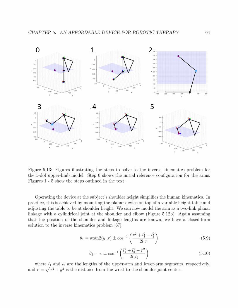
CHAPTER 5. AN AFFORDABLE DEVICE FOR ROBOTIC THERAPY 64
Figure 5.13: Figures illustrating the steps to solve to the inverse kinematics problem forthe 5-dof upper-limb model. Step 0 shows the initial reference configuration for the arms.Figures 1 - 5 show the steps outlined in the text.
Operating the device at the subject’s shoulder height simplifies the human kinematics. Inpractice, this is achieved by mounting the planar device on top of a variable height table andadjusting the table to be at shoulder height. We can now model the arm as a two-link planarlinkage with a cylindrical joint at the shoulder and elbow (Figure 5.12b). Again assumingthat the position of the shoulder and linkage lengths are known, we have a closed-formsolution to the inverse kinematics problem [67]:
θ1 = atan2(y, x)± cos−1
(r2 + l21 − l22
2l1r
)(5.9)
θ2 = π ± cos−1
(l21 + l22 − r2
2l1l2
)(5.10)
where l1 and l2 are the lengths of the upper-arm and lower-arm segments, respectively,and r =
√x2 + y2 is the distance from the wrist to the shoulder joint center.
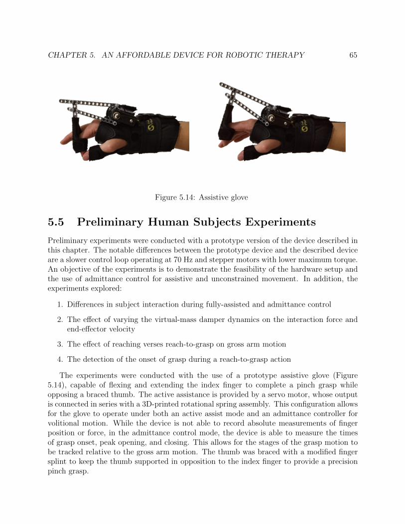
CHAPTER 5. AN AFFORDABLE DEVICE FOR ROBOTIC THERAPY 65
Figure 5.14: Assistive glove
5.5 Preliminary Human Subjects Experiments
Preliminary experiments were conducted with a prototype version of the device described inthis chapter. The notable differences between the prototype device and the described deviceare a slower control loop operating at 70 Hz and stepper motors with lower maximum torque.An objective of the experiments is to demonstrate the feasibility of the hardware setup andthe use of admittance control for assistive and unconstrained movement. In addition, theexperiments explored:
1. Differences in subject interaction during fully-assisted and admittance control
2. The effect of varying the virtual-mass damper dynamics on the interaction force andend-effector velocity
3. The effect of reaching verses reach-to-grasp on gross arm motion
4. The detection of the onset of grasp during a reach-to-grasp action
The experiments were conducted with the use of a prototype assistive glove (Figure5.14), capable of flexing and extending the index finger to complete a pinch grasp whileopposing a braced thumb. The active assistance is provided by a servo motor, whose outputis connected in series with a 3D-printed rotational spring assembly. This configuration allowsfor the glove to operate under both an active assist mode and an admittance controller forvolitional motion. While the device is not able to record absolute measurements of fingerposition or force, in the admittance control mode, the device is able to measure the timesof grasp onset, peak opening, and closing. This allows for the stages of the grasp motion tobe tracked relative to the gross arm motion. The thumb was braced with a modified fingersplint to keep the thumb supported in opposition to the index finger to provide a precisionpinch grasp.
CHAPTER 5. AN AFFORDABLE DEVICE FOR ROBOTIC THERAPY 66
Experimental Protocol
Data was collected from four control subjects and two subjects with upper limb impairmentunder approval of the UCSF Institutional Review Board with reliance approval by the UCBerkeley Institutional Review Board.
In the assisted mode, the device completes a linear minimum-jerk trajectory with noinput from the human subject. The minimum-jerk trajectory was selected to follow a smoothvelocity profile which has been found to describe a nominal trajectory for linear reaching[98]. For known start and end conditions and a specified duration, Hogan formulated theminimum jerk trajectory:
x(t) = xi + (xf − xi)(10(t/d)3 − 15(t/d)4 + 6(t/d)
)(5.11)
where xi is the initial position, xf is the final position, and d is the total duration of themotion. Note that we can independently compute the minimum-jerk trajectory for the xand y dimensions. To implement this we take the first derivative of the discrete-time versionof Equation 5.11 to compute the velocity based on the elapsed time. The trajectory iscomputed in real time with a proportional tracking term on the position error. In this mode,the human motion has no impact on the motion of the device. Subjects were instructed tofollow the motion of the device with their arm, and the interaction forces were recorded.In the admittance control mode, the subjects control the motion of the device through theinteraction force. Three combinations of mass and viscosity parameters were tested: A1)m = 3.3 kg, αv = 0.25, A2) m = 3.3 kg, αv = 0.5 A3) m = 2.2 kg, αv = 0.5.
All subjects were tested with their right arm in the device. This was the self-reporteddominant arm for all subjects. The device origin was positioned in front of the subject’sright shoulder joint center in the transverse plane. Targets were placed at three locations:at 0 degrees, 45 degrees, and 90 degrees from the origin. A foam ball of 1 in diameterwas connected to a weak magnetic mount. The vertical height of the mount was adjustedso that subjects could grasp the object when connected to the device. Prior to the startof the experiment, the reachable workspace of each subject was manually measured by theexperimenter along 8 radial lines from the origin. These measurements were used to set thereaching target distances along each of the target lines.
Trials were designated as reaching trials or reach-to grasp trials. During a reachingtrial, the subject completed only the gross reaching motion. During a reach-to-grasp trial,the subject either grasped or released the ball at the end of the reaching trajectory. Forall reach-to-grasp motions, the assistive glove operated under an admittance control mode.Each trial consisted of three outward reaches and three inward returns for each target.Each condition, reaching vs reach-to-grasp, assisted (two speeds), and admittance controlparameter (3 combinations) was completed once. Subjects were given time to rest betweensets of three trials.

CHAPTER 5. AN AFFORDABLE DEVICE FOR ROBOTIC THERAPY 67
Figure 5.15: Top-down view of planar reaching trajectories for control (left), post-stroke(center), and PLS (right) subjects. The color of each line corresponds to the velocity of thewrist at that point. Subjects performed series of reaches from the home position to radiallyplaced targets. The subject’s reachable workspace as measured by clinician is depicted ingray.
Results
Our analysis of this preliminary protocol is largely qualitative as the primary purpose wasto assess the hardware feasibility. Figure 5.15 shows sample reaching trajectories from trialsunder the admittance controller, comparing the motion of a representative control subject,a subject who is post-stroke, and a subject with early Primary Lateral Sclerosis (PLS). Weobserve variation in the velocity profile and peak speed during the gross transport phase, theability of the subject to stabilize their arm at the end of the motion, and the linearity andsmoothness of the reaching trajectory. These differences were noted despite the subject witha diagnosis of PLS having a high level of functional ability. On examination, this participanthad mild bilateral distal upper limb weakness (MRC scale 4/5), mildly elevated tone, andfull passive and active range of motion. Changes in the linearity of a reach or reach-to-grasptrajectory have been associated with cerebellar pathologies, leading to separation of themotions of the shoulder and elbow. Prior research has shown that the reaching motions ofpost-stroke subjects with upper limb impairment are slower, less accurate, and have poorercoordination than non-impaired individuals. Our anecdotal results appear to agree with

CHAPTER 5. AN AFFORDABLE DEVICE FOR ROBOTIC THERAPY 68
Figure 5.16: Preliminary observations from the human subject protocol. Top left: repre-sentative velocity plots for a single reaching motion for control subject (purple), post-strokesubject (blue), and subject with Primary Lateral Sclerosis (Red). Bottom left: demonstra-tion of feasibility to identify key stages of grasp during a reach-to-grasp motion. Right:representative trajectory for a forward reaching motion for a control subject (left) and apost-stroke subject (right), illustrating inability to stabilize at the trajectory endpoint.
these findings.Figure 5.16 summarizes several observations from the protocol. We show a sample veloc-
ity profile for a representative control subject and the two subjects with upper-limb impair-ment. The velocity profile for the control subjects has a higher peak velocity and exhibits theexpected bell-curve shape associated with a smooth, minimum-jerk trajectory. In contrast,the velocity of the two subjects with upper limb impairment does not have a single peak,but rather has a smaller period of acceleration followed by multiple peaks. This is morepronounced in the post-stroke subject than the subject with early PLS. This behavior isconsistent with the theory of submovments affecting movement smoothness following stroke[99]. The trajectory plots on the right of Figure 5.16 illustrate instability when the post-stroke subject attempted to remain steady at the end of a reaching motion. This instabilitywas not seen in any of the control subjects and indicates decreased ability to perform precisecontrol and regulate arm stiffness.

CHAPTER 5. AN AFFORDABLE DEVICE FOR ROBOTIC THERAPY 69
Figure 5.17: Bar charts showing mean peak force (left) and mean peak velocity (right) forhealthy controls subejcts completing reaching trials under the different admittance controllervirtual dynamics. Peak force and velocity values are normalized to the subject mean. Valuesrepresents the mean across the subjects with the error bar corresponding to inter-subjectvariance. The admittance mode virtual dynamics were defined by the following parameters:A1) m = 3.3 kg, αv = 0.25, A2) m = 3.3 kg, αv = 0.5 A3) m = 2.2 kg, αv = 0.5.
We demonstrate the ability to synchronize analysis of the global reaching motion withthe action of the hand (Figure 5.16). Based on position data recorded from the glove device,we identify four key points in the grasping motion: 1) initial hand motion, 2)begin fullyopen, 3) fully open, 4) begin closing. Because of the small difference in position betweenbeginning to close and the final closed position, it was difficult to identify the time of graspcompletion. This is a limitation of the low resolution of the position sensing of the glovedevice. Information of the grasping motion related to the reaching motion is useful in thestudy of motor recovery following stroke. In normal reach-to-grasp motion, subjects preshapethe hand prior to reaching the end of the reaching trajectory to prepare to grasp the object.Quantitative analysis of these onset times is not included.
Finally, we analyze the effect of altering the virtual dynamics for the admittance controltrials for the control subjects. We consider two values: the peak interaction force and thepeak velocity for each reaching motion. We compare the values for outward reaching tothe target at 45 degrees. To analyze trends across subjects, the values for each subject arenormalized with respect to the subjects mean value across each trial. The mean values areshown in Figure 5.17 with the standard deviation corresponding to the variance between

CHAPTER 5. AN AFFORDABLE DEVICE FOR ROBOTIC THERAPY 70
subjects. A1, the controller with a heavier virtual mass, has a higher mean peak force and alower mean peak velocity. These results demonstrate that it is possible to alter the humaninteraction with the device by altering the virtual dynamics. We asked subjects for theirpreference among the three admittance control virtual dynamics. Of note, all healthy controlsubjects selected either A2 or A3, citing the ability to move at a faster speed. Both subjectswith upper limb impairment selected A1. For both subjects, A1 required more force andtook a longer period of time to complete the motion. However subjects cited feeling morestable as the reason for their preference.
5.6 Simulation Case Study: Effect of Passive Flexor
Muscle Tightness on Joint Torques During Planar
Arm Reaching
We now consider the incorporation of a muscle model into our analysis with the developedsystem. Preliminary reaching data from a Spinal Cord Injury (SCI) subject was collectedunder approval of the UCSF Institutional Review Board. Example data is shown in Figure5.18. With the goal of using this robotic device to assess function and assist motion, thisstudy implements a simple biomechanical model which can be incorporated in the analysisof data from the device. Spinal Cord Injury (SCI) may result in impaired function of theupper limb including decreased range of motion due to an increased passive stiffness of theflexor muscles accompanied by deficits in strength. In this case study, we utilize a six-musclemodel of the arm to simulate passive muscle forces during reaching motions in the horizontalplane. We study the effect of muscle-level tightness on the resultant elbow and shouldertorques throughout the arm workspace. The resulting joint torques exhibit an expectedincrease with greater muscle tightness, with this effect most pronounced in lateral reachingmotions. These results demonstrate initial feasibility of the use of a simplified muscle modelto study joint effects of muscle-tightness, providing insight towards the future developmentof assessment protocols for generating individualized models of function from task-spaceobservations. Alongside deficits in strength and motor control, SCI may result in tightnessof the flexor muscles, resulting in a decrease in range of motion [100]. An increase in passivemuscle stiffness and connective tissue of the flexors must be overcome by the active muscleforce of the opposing extensor muscles. In this work, we study the effects of muscle tightnesson the resultant joint-torques from passive muscle forces during static reaching. This analysisprovides insight into how the passive component of muscle force manifests in the joint andtask space.
Methods
We consider a two-link model of the upper-limb (right arm) with rotational joints at theshoulder and elbow. Motion is constrained to the tranverse plane at shoulder-height, and

CHAPTER 5. AN AFFORDABLE DEVICE FOR ROBOTIC THERAPY 71
Figure 5.18: Left: representative reaching data from a subject with spinal cord injury un-dergoing passive reaching to three radial targets. Wrist position is shown in black with theinteraction force shown as the scaled red vector. Right: musculosketal arm model. Figurefrom [101].
Figure 5.19: (Left) Passive muscle force vs. muscle length. Relationship is shown for fourvalues of nominal muscle length l0. (Right) Simulated wrist positions for reaching trajectoriesin Cartesian space.
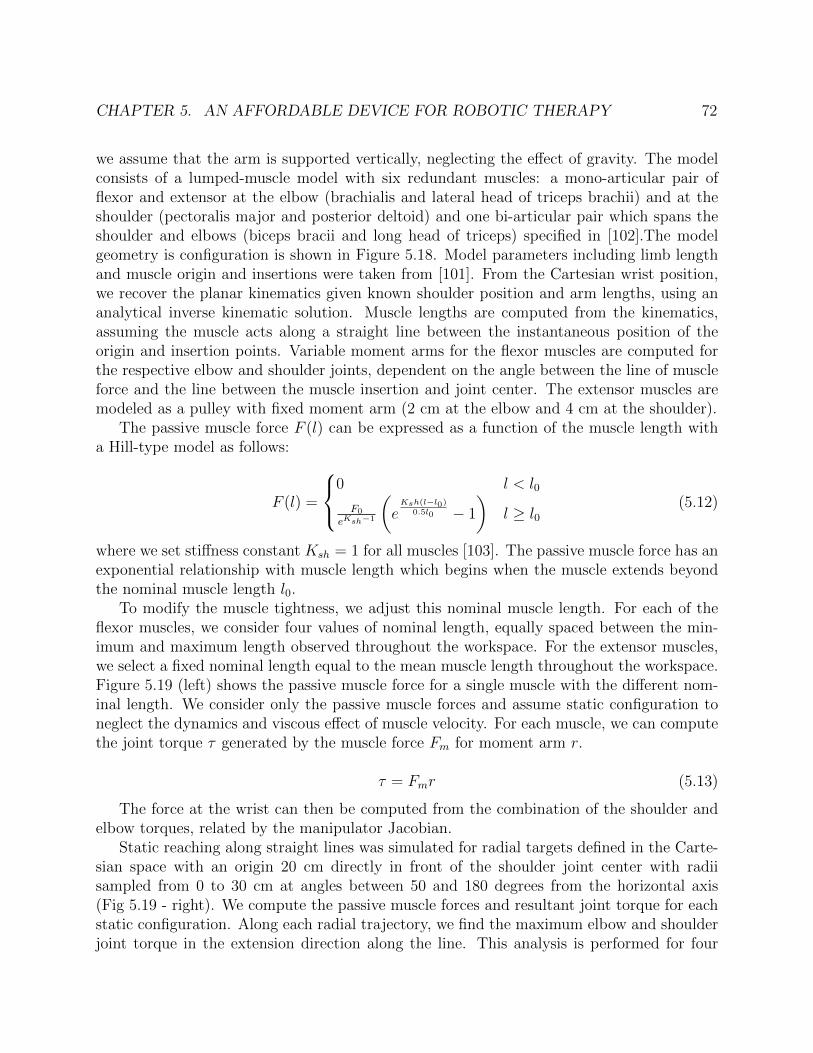
CHAPTER 5. AN AFFORDABLE DEVICE FOR ROBOTIC THERAPY 72
we assume that the arm is supported vertically, neglecting the effect of gravity. The modelconsists of a lumped-muscle model with six redundant muscles: a mono-articular pair offlexor and extensor at the elbow (brachialis and lateral head of triceps brachii) and at theshoulder (pectoralis major and posterior deltoid) and one bi-articular pair which spans theshoulder and elbows (biceps bracii and long head of triceps) specified in [102].The modelgeometry is configuration is shown in Figure 5.18. Model parameters including limb lengthand muscle origin and insertions were taken from [101]. From the Cartesian wrist position,we recover the planar kinematics given known shoulder position and arm lengths, using ananalytical inverse kinematic solution. Muscle lengths are computed from the kinematics,assuming the muscle acts along a straight line between the instantaneous position of theorigin and insertion points. Variable moment arms for the flexor muscles are computed forthe respective elbow and shoulder joints, dependent on the angle between the line of muscleforce and the line between the muscle insertion and joint center. The extensor muscles aremodeled as a pulley with fixed moment arm (2 cm at the elbow and 4 cm at the shoulder).
The passive muscle force F (l) can be expressed as a function of the muscle length witha Hill-type model as follows:
F (l) =
0 l < l0
F0
eKsh−1
(e
Ksh(l−l0)0.5l0 − 1
)l ≥ l0
(5.12)
where we set stiffness constant Ksh = 1 for all muscles [103]. The passive muscle force has anexponential relationship with muscle length which begins when the muscle extends beyondthe nominal muscle length l0.
To modify the muscle tightness, we adjust this nominal muscle length. For each of theflexor muscles, we consider four values of nominal length, equally spaced between the min-imum and maximum length observed throughout the workspace. For the extensor muscles,we select a fixed nominal length equal to the mean muscle length throughout the workspace.Figure 5.19 (left) shows the passive muscle force for a single muscle with the different nom-inal length. We consider only the passive muscle forces and assume static configuration toneglect the dynamics and viscous effect of muscle velocity. For each muscle, we can computethe joint torque τ generated by the muscle force Fm for moment arm r.
τ = Fmr (5.13)
The force at the wrist can then be computed from the combination of the shoulder andelbow torques, related by the manipulator Jacobian.
Static reaching along straight lines was simulated for radial targets defined in the Carte-sian space with an origin 20 cm directly in front of the shoulder joint center with radiisampled from 0 to 30 cm at angles between 50 and 180 degrees from the horizontal axis(Fig 5.19 - right). We compute the passive muscle forces and resultant joint torque for eachstatic configuration. Along each radial trajectory, we find the maximum elbow and shoulderjoint torque in the extension direction along the line. This analysis is performed for four

CHAPTER 5. AN AFFORDABLE DEVICE FOR ROBOTIC THERAPY 73
Figure 5.20: Kinematic configuration at three arm configurations along reaching trajectoriesin the left, center, and right directions. Arm links are shown in black with flexor muscles inred and extensor muscles in blue. The reaching trajectory is shown as the dashed line.
nominal muscle for each of the mono-articular elbow flexor, shoulder flexor, and bi-articularflexor individually and for increased tightness and all three flexors. All computations werecompleted in MATLAB 2017a.
Representative kinematic configurations of the arm model are shown in Figure 5.20,illustrating the changes in muscles length. The maximum resultant joint torques for thefour muscle tightness conditions are shown in Figure 5.21. Adjusting the nominal musclelength of the shoulder flexors has expected changes in shoulder torque and does not affect theelbow torque. The same effect is observed when only the elbow flexor tightness is modified.Adjusting the tightness of the bi-articular muscle results in torque effects in both the shoulderand elbow. The greatest torque is seen when all three flexor muscles have increased tightness.
Discussion
We implemented an upper limb musculoskeletal model with six muscles to assess the effectof passive muscle tightness on joint torques. The results demonstrate expected increasesin elbow and shoulder torques with increases in flexor muscle tightness. The effect of thebi-articular muscle on both elbow and shoulder joints indicates a usefulness in the incorpo-ration of a muscle-level model in this analysis rather than a simple rotational stiffness at thejoint-level. Additionally, the effects of the muscle parameters are observed to vary withinthe workspace, with greater torque at the most lateral target as both the shoulder and elbowflexors are extended in this arm configuration. This result implies that it is valuable to con-sider mechanical constraints at the muscle-level effects when developing controllers that willoperate in the Cartesian workspace. Assessment of active range of motion, convey limitationsdue to a combination of passive stiffness and deficits in active muscle force generation Theanalysis in the study is limited as we consider only the passive component of muscle forcefor a simplified muscle model. The total muscle force must be modeled as a combination of
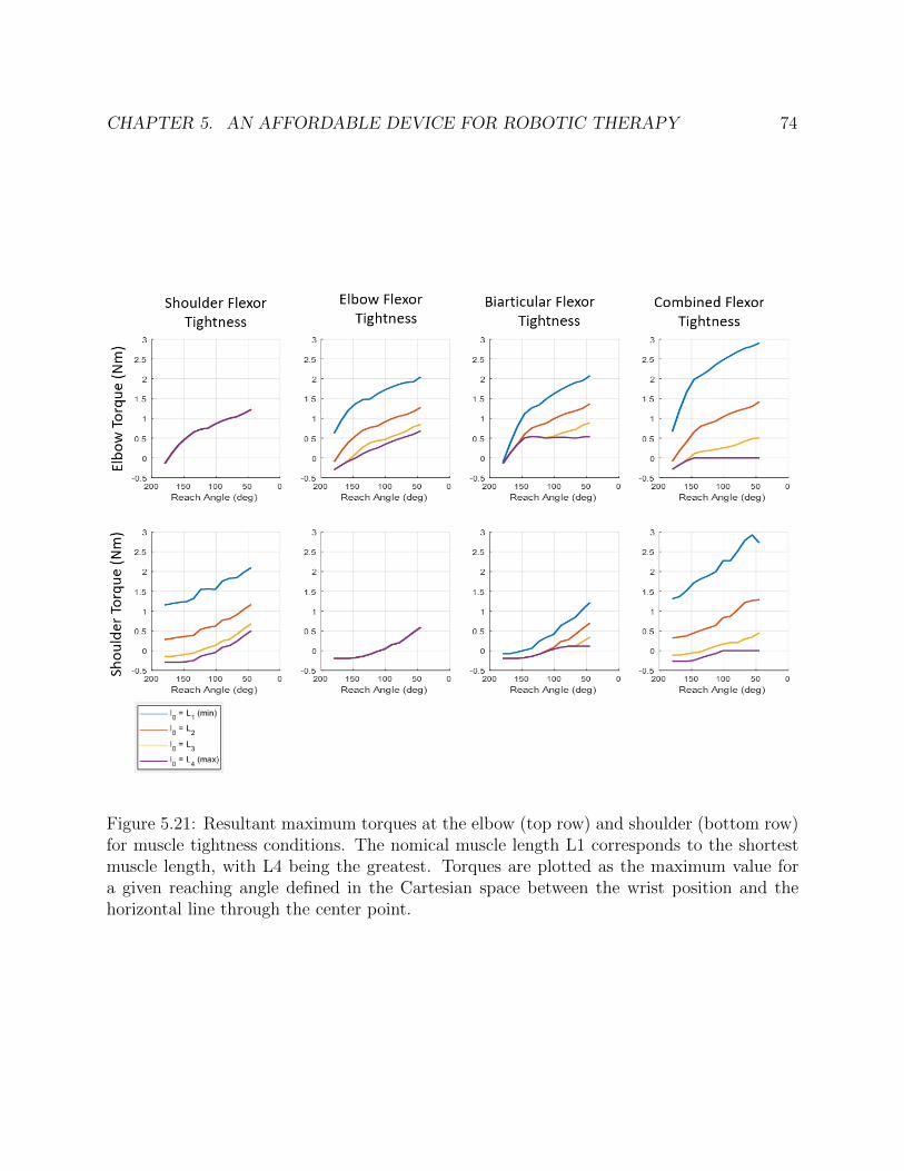
CHAPTER 5. AN AFFORDABLE DEVICE FOR ROBOTIC THERAPY 74
Figure 5.21: Resultant maximum torques at the elbow (top row) and shoulder (bottom row)for muscle tightness conditions. The nomical muscle length L1 corresponds to the shortestmuscle length, with L4 being the greatest. Torques are plotted as the maximum value fora given reaching angle defined in the Cartesian space between the wrist position and thehorizontal line through the center point.
CHAPTER 5. AN AFFORDABLE DEVICE FOR ROBOTIC THERAPY 75
active and passive muscle forces. While it is straightforward to implement the forward modelwith specified values of nominal muscle length, it is difficult to separately assess the passiveand active components of muscle force. However, given the joint-specific and workspacevariations, the preliminary results of this parameter study indicate that for passive motionwe may be able to identify optimal muscle-model parameters which correspond to the ob-served end-effector forces. Future work will aim to utilize this model of passive muscle forcesto drive subject specific models of impairment using task-space observations of motion andforce with a planar robotic device.
5.7 Chapter Summary
This chapter presented the design, analysis, and validation of an affordable planar roboticdevice for upper limb assessment and rehabilitation. With a total material cost of lessthan $800, the device was able to meet our design objectives. We introduce a novel con-figuration for low-cost load cells, enabling measurement of human-robot interaction forces.The measured forces and positions recorded by the device were experimentally validatedagainst ground truth measurements. Initial human subjects experiments demonstrated de-vice feasibility through the subject ability to operate the device under volitional force-basedadmittance control. We observed differences in the robot interaction of healthy control sub-jects and subjects with a low-level of impairment, with notable differences in peak forcesand velocities, motion smoothness, the ability to stabilize, and the self-selected preferablevirtual dynamics.

76
Chapter 6
Algorithms for Assistance andAssessment
In this chapter, we utilize the robotic device developed in Chapter 5 to investigate two meth-ods for assisting and assessing human motion: 1) the use of lateral spring assistance duringelliptical trajectory tracing and 2) the assessment of arm strength through isolated jointmotions. We describe our motivation, design, and implementation for each of protocol andpresent analysis of human subject data. These results further demonstrate the capabilitiesof the affordable device for quantitative assessment and robotic therapy applications.
6.1 Exploitation of Assistance During Ellipse Tracing
Motivation and Background
During the preliminary experiments (Section 5.5), we observed a behavior in which subjectswere leaning into a virtual safety wall by exerting a large interaction force in the directionof the wall, normal to the direction of the desired trajectory. Subjects were not generallyassisted in completing the protocol under an admittance controller. There were, however,force fields at the edge of the human workspace which prevented the subject from reachingoutside of a safe region. The target to the left was positioned along the virtual wall, with astraight line from the starting point to the target running along the wall. This unintentionallyresulted in several subjects exploiting the presence of the virtual wall by exerting a forcein the direction of the wall to maintain a stable trajectory. An example of this behavior isshown in Figure 6.1. This figure shows data from a subject with upper-limb impairment,following diagnosis of Primary Lateral Sclerosis. Here we observe variance in the positiontrajectories for the vertical and 45 degree targets. The left target of interest has almost novariance. Additionally, from the overlaid velocity profile, we observe higher peak velocitiesalong the left target, indicating higher forces directed along the line of interest. This can beexplained by the plot to the right which shows the interaction force exerted by the subject.
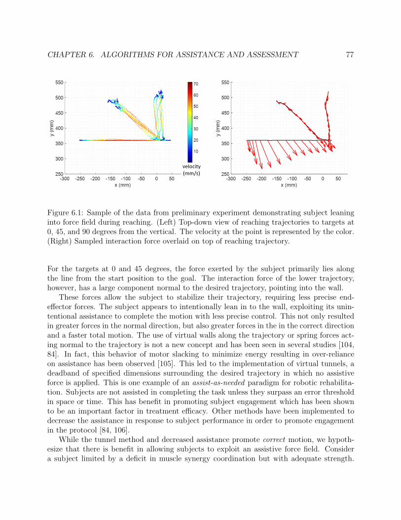
CHAPTER 6. ALGORITHMS FOR ASSISTANCE AND ASSESSMENT 77
Figure 6.1: Sample of the data from preliminary experiment demonstrating subject leaninginto force field during reaching. (Left) Top-down view of reaching trajectories to targets at0, 45, and 90 degrees from the vertical. The velocity at the point is represented by the color.(Right) Sampled interaction force overlaid on top of reaching trajectory.
For the targets at 0 and 45 degrees, the force exerted by the subject primarily lies alongthe line from the start position to the goal. The interaction force of the lower trajectory,however, has a large component normal to the desired trajectory, pointing into the wall.
These forces allow the subject to stabilize their trajectory, requiring less precise end-effector forces. The subject appears to intentionally lean in to the wall, exploiting its unin-tentional assistance to complete the motion with less precise control. This not only resultedin greater forces in the normal direction, but also greater forces in the in the correct directionand a faster total motion. The use of virtual walls along the trajectory or spring forces act-ing normal to the trajectory is not a new concept and has been seen in several studies [104,84]. In fact, this behavior of motor slacking to minimize energy resulting in over-relianceon assistance has been observed [105]. This led to the implementation of virtual tunnels, adeadband of specified dimensions surrounding the desired trajectory in which no assistiveforce is applied. This is one example of an assist-as-needed paradigm for robotic rehabilita-tion. Subjects are not assisted in completing the task unless they surpass an error thresholdin space or time. This has benefit in promoting subject engagement which has been shownto be an important factor in treatment efficacy. Other methods have been implemented todecrease the assistance in response to subject performance in order to promote engagementin the protocol [84, 106].
While the tunnel method and decreased assistance promote correct motion, we hypoth-esize that there is benefit in allowing subjects to exploit an assistive force field. Considera subject limited by a deficit in muscle synergy coordination but with adequate strength.

CHAPTER 6. ALGORITHMS FOR ASSISTANCE AND ASSESSMENT 78
Figure 6.2: Left: drawing of the tangent-normal coordinate frame for linear spring assistance,showing the unit and normal tangent vectors, un and ut, current position p and desiredposition d. Right: plot of the vector field of the linear spring assistance for a linear desiredtrajectory.
Operating within the deadband of a tunnel, the subject may complete slow, disjoint motionsdue to their inability to precisely regulate the direction of their end-effector force output.With an assistive wall, we hypothesize that the subject may be able to more confidentlyexert greater force and complete a faster, smoother motion. We present an experiment toinvestigate this approach when applied to continuous elliptical trajectories.
6.2 Spring Assistance Formulation
Building on the free admittance control framework presented in section 5.4, we incorporatean assistive spring term into the mass-damper virtual dynamics model. In this section, wefirst explain the controller implementation for a linear trajectory and then expand to theelliptical trajectories studied in this chapter. We consider a desired trajectory with a spatialcomponent and no specified velocity profile for self-paced motion under admittance control.The assistance helps the subject follow the desired trajectory by applying a restoring forcewhen the subject deviates from the trajectory. We implement this through a virtual linearspring acting in the direction normal to the trajectory. If the subject has no position error,the spring will provide zero force. Likewise, the spring provides no assistance along theforward direction of the trajectory. This type of assistance does not perform the task for thesubject but, rather, assists in error correction. A linear spring was selected rather than ahard virtual wall to allow for some deviation without a strong restoring force. While we didnot implement a virtual tunnel deadband to encourage the exploitation of the assistance, itwould be straightforward to incorporate a deadband as an alternative protocol.

CHAPTER 6. ALGORITHMS FOR ASSISTANCE AND ASSESSMENT 79
To implement these dynamics, we first perform a transformation from the device Carte-sian coordinate system into the instantaneous tangent-normal coordinate frame of the desiredtrajectory. The normal vector is perpendicular to the tangent vector at a counterclockwiserotation of 90 degrees. We define the unit tangent vector ut and unit normal vector un tobe tangent and normal to the trajectory. For a line, the tangent-normal frame has fixed ori-entation with the tangent axis colinear with the trajectory. The spring acts in the directionof un with force proportional to the distance from the trajectory along un:
Fspring = −k (p− d) · un (6.1)
where p is the current position, d is the nearest position on the desired trajectory, and k isa spring constant chosen for selected stiffness level. Note that the formulation of this springforce differs slightly from the standard form [107] through the vector dot product with theunit normal vector. Our formulation was selected for expansion to elliptical trajectorieswhen the approximated unit normal vector may not be collinear with p − d. We nowrepresent our admittance controller with virtual mass-spring-damper dynamics in tangentnormal coordinates:
Fn = mxn(t) + cxn(t)− k(p− d) · un (6.2)
Ft = mxt(t) + cxt(t) (6.3)
where the subscripts n and t denote the normal and tangent directions for the force, acceler-ation, and velocity. Note that there is no spring force in the tangent direction. The virtualmass and damper constants are the same for the normal and tangent directions. Controllervelocities computed in the normal-tangent frame are transformed to the Cartesian frame.
Spring Assistance for an Elliptical Trajectory
Implementation of the linear spring force on an elliptical trajectory requires computation ofthe instantaneous tangent and normal vectors to the ellipse at a given point. Consider astandard ellipse defined the following parametric equation:[
xy
]=
[a cos (t)b sin (t)
](6.4)
for 0 ≤ t ≤ 2π, where x and y correspond to the position, a is the length of the semi-majoraxis, and b is the length of the semi-minor axis. We derive the tangent to an ellipse at apoint d which lies on the ellipse. The slope of the tangent line is the first derivative at thepoint. First, take the first derivative of Eq. 6.4:[
xy
]=
[a sin (t)b cos (t)
](6.5)

CHAPTER 6. ALGORITHMS FOR ASSISTANCE AND ASSESSMENT 80
Figure 6.3: Illustration of the method for determining the unit tangent vector ut and unitnormal vectorun at a point p when tracking an elliptical trajectory. (Left) Finding thedesired point d, (Center) Computing the unit tangent and unit normal vectors at the desiredposition, (Right) Translating the tangent-normal coordinate frame to the current position.
Rearranging Eq. 6.4, we have cos(t) = x/a and sin(t) = y/b. These relationships arecombined with 6.5 to obtain the tangent vector vt:
vt =
[−aybbxa
](6.6)
and unit tangent vector:
ut =vt
‖vt‖=
−a2y√a4y2+b4x2
b2x√a4y2+b4x2
(6.7)
The unit normal vector is perpendicular to the unit tangent vector, pointing into thecurve. We can compute the unit normal with the following equation:
un =
[−uty
utx
]=
−b2x√a4y2+b4x2
−a2y√a4y2+b4x2
(6.8)
We transform the forces measured in the Cartesian frame into the tangent-normal framewith the equation: [
ftfn
]=[ut un
]T [fxfy
](6.9)
CHAPTER 6. ALGORITHMS FOR ASSISTANCE AND ASSESSMENT 81
For a point p which does not lie on the ellipse, we select the desired point d on theellipse to be the intersection of the ellipse and a line between p and o, the ellipse origin. Theposition of the point d is expressed by the equation:
d =
[abpx
a2p+y2+b2p2xabpy
a2p+y2+b2p2x
](6.10)
Note that for the general case of an ellipse, the point d is not the closest point to theellipse, but rather it is along the radial line from the origin. For the specific case of a circle,these points will be the same. The closest point to the ellipse does not have a closed-formsolution. It can be solved with numerical optimization, but this was not chosen for ourimplementation to decrease the computational complexity as these constraints are beingperformed in realtime on an inexpensive microcontroller. We compute the unit tangent andunit normal vectors at the point d. These vectors approximate the unit tangent and normalvector for the point p which is not on the ellipse. The spring force acts along the unit normalvector from the point p toward the elliptical path. The vector field of spring force is plottedin Figure 6.4.
6.3 Experimental Protocol
Our experimental protocol was selected to study human interaction with the system underassisted and unassisted control. We hypothesize that the presence of a stiff assistive force fieldwill result in the leaning in behavior observed in the linear reaching experiments. Subjectscompleted ellipsoidal trajectories with the device operating under an admittance controller.We consider three independent variables: admittance control virtual mass, spring assistance,and ellipse orientation. Two values of virtual mass (0.47 kg and 0.92 kg) were selected. Thelower mass provides a lighter, more transparent motion. This lighter mass was selected tobe so light that it may feel slightly unstable but not result in significant oscillations. Thefour ellipse orientations are rotations of 0, 45, 90, and -45 degrees from the vertical. Asingle spring constant of ks = 1 was selected for the assisted case. No spring force wasapplied for the unassisted case. The combinations of variables correspond to a total of 16unique test conditions. Subjects completed 3 trials of each of conditions, resulting in 48total trials. Note that one subject completed only 32 trials (two of each condition) due to atime constraint on the part of the subject. Trials were broken into blocks of four trials whichconsisted of one trial for each ellipse orientation for a given mass and assistance condition.Subjects were informed if the trial would be assisted or unassisted. The order of the ellipseorientation was randomized. Each trial consisted of 10 ellipses, beginning and ending atthe vertex. The ellipses were defined by semi-major axis a = 100 and semi-minor axis b= 50. The first and last ellipse were excluded from each trial during analysis to accountfor effects of initial acceleration or adjustment and final deceleration. All trajectories werecompleted in a counter-clockwise direction. The desired ellipse was displayed on a monitor

CHAPTER 6. ALGORITHMS FOR ASSISTANCE AND ASSESSMENT 82
Figure 6.4: Vector field plot of the assistive spring force field for an elliptical trajectory.Arrows indicated the magnitude and direction of the force for the given position error fromthe desired trajectory.
in from of the subject, with visual feedback of the current wrist position shown as a reddot (Figure 6.5). Subjects were instructed to trace the path of the ellipse and move at acomfortable and continuous pace for the duration of the trial (not stopping at the end ofeach ellipse). Position, velocity, and force data was collected from the device. Position datawas also collected from a motion capture system (Phasespace Impulse X2) at 480 Hz.
Data was collected from seven young adult subjects (4 M, 3 F) with no upper-limbimpairment at UC Berkeley under the approval of the UCSF Institutional Review Boardwith reliance approval by the UC Berkeley Reliance Registry. The right arm of each subjectwas tested. This was the self-identified dominant hand of six of the seven subjects.
6.4 Results
Analysis Methodology
We consider several metrics for analyzing the effect of virtual mass, assistance, and orienta-tion on the elliptical trajectory tracing. These metrics are computed from the position and

CHAPTER 6. ALGORITHMS FOR ASSISTANCE AND ASSESSMENT 83
Figure 6.5: Subject connected to rehabilitation device. The monitor displays the desiredtrajectory and real-time feedback of the subject’s wrist position.
force data measured by the device at 330 Hz. The motion capture system was not used inthe computation of these metrics. Analysis was completed offline in MATLAB. A 3rd orderlowpass Butterworth filter with a 6 Hz cutoff frequency was applied to the x and y compo-nents of the force data. The position data was not filtered. Each trial was segmented intoindividual ellipses for analysis. The following metrics were used to process the experimentaldata:
� Normalized mean force (NMF). We define the mean force (MF) of an ellipse tobe the mean value of the magnitude of the interaction force vector across time
MF =1
K
K∑k=1
‖f(k‖ (6.11)
where f(k) is the force vector at timestep k and K is the number of samples in theellipse. Between subjects, there was variation in the mean interaction force. To assesstrends across the subjects, we normalize the mean force for an ellipse by scaling it tothe subjects’s mean force across all trials:
NMF (t) =MF (t)
MF(6.12)
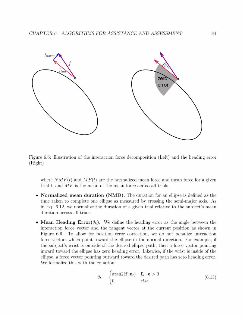
CHAPTER 6. ALGORITHMS FOR ASSISTANCE AND ASSESSMENT 84
Figure 6.6: Illustration of the interaction force decomposition (Left) and the heading error(Right)
where NMF (t) and MF (t) are the normalized mean force and mean force for a giventrial t, and MF is the mean of the mean force across all trials.
� Normalized mean duration (NMD). The duration for an ellipse is defined as thetime taken to complete one ellipse as measured by crossing the semi-major axis. Asin Eq. 6.12, we normalize the duration of a given trial relative to the subject’s meanduration across all trials.
� Mean Heading Error(θh). We define the heading error as the angle between theinteraction force vector and the tangent vector at the current position as shown inFigure 6.6. To allow for position error correction, we do not penalize interactionforce vectors which point toward the ellipse in the normal direction. For example, ifthe subject’s wrist is outside of the desired ellipse path, then a force vector pointinginward toward the ellipse has zero heading error. Likewise, if the wrist is inside of theellipse, a force vector pointing outward toward the desired path has zero heading error.We formalize this with the equation:
θh =
{atan2(f ,ut) fn · e > 0
0 else(6.13)

CHAPTER 6. ALGORITHMS FOR ASSISTANCE AND ASSESSMENT 85
where e is the error vector between the current position p and the desired position d.
� Zero crossings of the normal force Zero crossings in the normal force can beindicative of position error correction. The number of zero crossings is counted perellipse.
� Coefficients of velocity-curvature Ellipses provide an opportunity to investigatethe relationship between velocity and path curvature. Studied have found that continu-ous human movements follows the Two-Thirds Power Law which states that end-pointvelocity (V) is a power function of the radius of curvature of the endpoint trajectory.The kinematics of this relationship have been studied outside of robotic devices [108],with a study of the relationship in water [109]. The ability of the robotic device toadjust the virtual mass and viscosity parameters allows for testing of this relationshipunder loading. Recently, the interaction forces between a robot and human were stud-ied when humans follow robot motion along intuitive and unintuitive velocity profiles[110].
Changes in Ellipse Tracking
We first describe qualitative observations from the experiment. Figure 6.7 shows representa-tive results from a subject completing elliptical trials under unassisted and assisted conditionsfor the light admittance mass. The data represents a single ellipse of each condition for anellipse at a rotation of 90 degrees under the light admittance mode. The top row shows anexample position trajectory with the color corresponding to the velocity at that point. Thesampled interaction force exerted by the subject at the wrist is shown by the black vectors.Comparing the total interaction force in the unassisted and assisted case, we observe thatthe magnitude of the interaction force is greater in the assisted case, corresponding to ahigher velocities. Looking at the normal force, in the unassisted case, we observe that thedirection of the force changes sign as the subject adjusts the direction of the interaction forcein order to correct for position error. In the unassisted case, we observe that the normalforce has a greater magnitude when compared to the unassisted case and the direction of thenormal force points outward for the entirety of the trial. This direction indicates that thesubject is not carefully modulating the direction of their exerted force in order to follow thetrajectory, but, rather is leaning into the spring force to achieve smooth motion. We notethat this constant outward direction is not consistent for this subject among all conditions,or between subjects. In studying these force plots, we observe subjects with normal forcepointed continuously inward, normal force with a bias in the task space (ie. majority directedupward), or normal force which changes direction throughout the ellipse. For a given trialof the same orientation and controller parameters, subjects tend to follow the same patternof normal force direction for each of the ten ellipses.
These qualitative observations are supported by the quantitative metrics shown in Figure6.8 and Table 6.1. These mean metrics are averaged across all subjects with standard
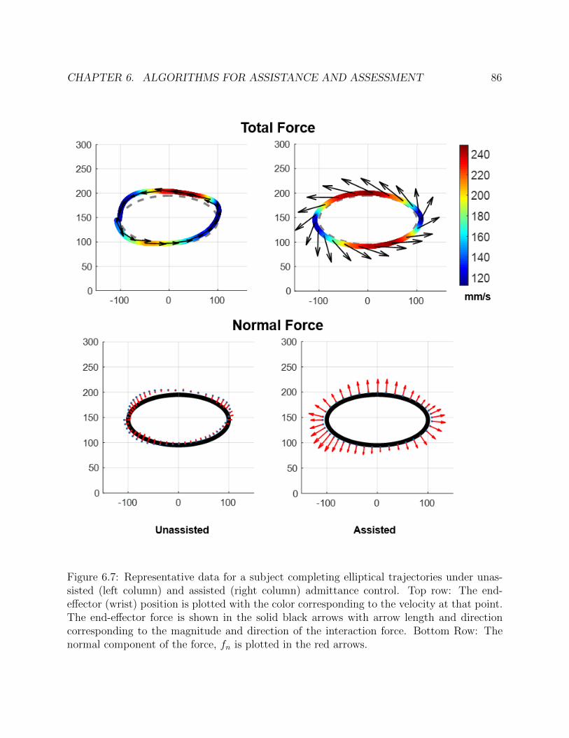
CHAPTER 6. ALGORITHMS FOR ASSISTANCE AND ASSESSMENT 86
Figure 6.7: Representative data for a subject completing elliptical trajectories under unas-sisted (left column) and assisted (right column) admittance control. Top row: The end-effector (wrist) position is plotted with the color corresponding to the velocity at that point.The end-effector force is shown in the solid black arrows with arrow length and directioncorresponding to the magnitude and direction of the interaction force. Bottom Row: Thenormal component of the force, fn is plotted in the red arrows.

CHAPTER 6. ALGORITHMS FOR ASSISTANCE AND ASSESSMENT 87
Figure 6.8: Bar charts of the results of of ellipse tracking, showing the mean normalizedforce (left), mean normalized duration (center), and mean heading error.
Table 6.1: Quantitative interaction metrics under four virtual dynamic conditions: LightUnassisted (LU), Light Assisted (LA), Heavy Unassisted (HU), and Heavy Assisted (HA).The mean is taken across all subjects with the standard deviation corresponding to varianceacross subjects.
Metric LU LA HU HANorm. Mean Force 0.60 ± 0.06 0.9 ± 0.09 1.07 ± 0.11 1.41 ± 0.08
Norm. Duration 1.14 ± 0.10 0.84 ± 0.07 1.10 ± 0.09 0.90±0.06Mean Heading Error 4.93 ± 2.97 10.32 ± 4.24 4.21 ± 2.41 8.05 ± 2.21
Zero Crossings 5.77 ± 3.99 3.22 ± 1.35 4.89 ±3.37 3.2 ± 1.39
Table 6.2: Mean force for each subject under four virtual dynamic conditions: Light Unas-sisted, Light Assisted, Heavy Unassisted, and Heavy Assisted. The mean and standarddeviation are taken across all trials for the condition (all orientations).
Subject Light Unassisted Light Assisted Heavy Unassisted Heavy AssistedS01 8.14 ± 1.79 16.23 ± 4.94 12.55 ± 1.82 22.30 ± 4.43S02 2.96 ± 0.34 4.09 ± 0.63 5.04 ± 0.67 6.98±1.28S03 5.11 ± 1.33 8.37 ± 1.54 10.82 ± 1.79 14.07 ± 2.12S04 6.70 ± 0.59 8.77 ± 0.93 11.29 ±0.74 13.04 ± 1.47S05 4.80 ± 0.98 7.98 ±0.87 9.72 ±1.01 12.69 ±1.46S06 5.85 ± 0.70 8.47 ± 1.64 9.46 ± 0.91 12.99 ±1.57S07 3.28 ±0.31 4.09 ± 0.47 6.06 ±0.34 6.63 ± 0.53

CHAPTER 6. ALGORITHMS FOR ASSISTANCE AND ASSESSMENT 88
deviation representing inter-subject variation. These metrics are also averaged across allorientations as no significant difference was found between the orientations when averagedacross all subjects. There were significant differences between the orientations for individualsubjects, but these were not found to be trends across subjects. The results show a greatermean normalized forced in the assisted case than the unassisted case for both the light andheavy conditions, indicating that subjects are exerting greater active forces with the presenceof spring assistance. The mean normalized duration decreases in the unassisted case forboth light and heavy conditions, corresponding with the increase in interaction force. Withthe assistance, subjects are completing each ellipse in less time. The mean heading errorincreases in the assisted case for both the light and heavy conditions. When comparing thelight and heavy condition, the normalized total force increases under the heavier condition.The normalized duration, however, is unaffected by the virtual mass. For the unassistedcase, the mean heading error is unaffected by the virtual mass. However, in the assistedcase, the mean heading error is greater for the lighter mass.
These results support the hypothesis that subjects will exploit assistance when completingthe task as demonstrated by the increase in the heading error. This is also supported bythe decrease in zero-crossings in the assisted case. Figure 6.9 shows an example plot ofthe normal force, highlighting the frequency of zeros crossings in the unassisted case. Thisvaried between subjects with two subjects exhibiting slower, more precise motion. Althoughthe healthy control subjects are capable of completing the task with minimal heading erroras demonstrated in the unassissted case, we see a reliance on the assistive force field. Theresults support the hypothesis that the force field will result in greater exertion as evidencedby the increase in greater mean force and decreased duration.
We note that there were significant difference in the mean force exerted by each subjectwhich are shown in Table 6.2. Despite these differences in the magnitude of force, the trendsin the normalized forces were seen across subjects.
Human Arm Inverse Kinematics and Statics Analysis
Thus far, we have only considered metrics relating to the end-effector position, velocity andforce. The end-effector measures correspond to motion and torques exerted by the humanarm. The inverse kinematic method described in section 5.4 can be used to estimate thejoint angles from the device measurement alone (with additional measurement of shoulderjoint center and limb segment length). In this study, however, we use active motion capturedata to recover the joint angles. The method used is similar to that described in Chapter 2.For each subject, we first utilize an optimization-based parameter identification method torecover an individualized rigid body model. The recovered model consists of three segmentsin the transverse plane with a torso base segment and two segments for the upper and lowerarms which are connected by cylindrical joints corresponding to the shoulder and elbow.The parameter-identification method optimizes for the rigid body parameters which definethe model and the positions of the motion capture markers in the local segment frame. Theend-effector position recorded by the device was integrated into the optimization and treated
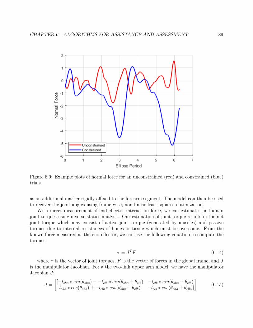
CHAPTER 6. ALGORITHMS FOR ASSISTANCE AND ASSESSMENT 89
Figure 6.9: Example plots of normal force for an unconstrained (red) and constrained (blue)trials.
as an additional marker rigidly affixed to the forearm segment. The model can then be usedto recover the joint angles using frame-wise, non-linear least squares optimization.
With direct measurement of end-effector interaction force, we can estimate the humanjoint torques using inverse statics analysis. Our estimation of joint torque results in the netjoint torque which may consist of active joint torque (generated by muscles) and passivetorques due to internal resistances of bones or tissue which must be overcome. From theknown force measured at the end-effector, we can use the following equation to compute thetorques:
τ = JTF (6.14)
where τ is the vector of joint torques, F is the vector of forces in the global frame, and Jis the manipulator Jacobian. For a the two-link upper arm model, we have the manipulatorJacobian J :
J =
[[−lsho ∗ sin(θsho)−−lelb ∗ sin(θsho + θelb) −lelb ∗ sin(θsho + θelb)lsho ∗ cos(θsho) +−lelb ∗ cos(θsho + θelb) −lelb ∗ cos(θsho + θelb)]
](6.15)
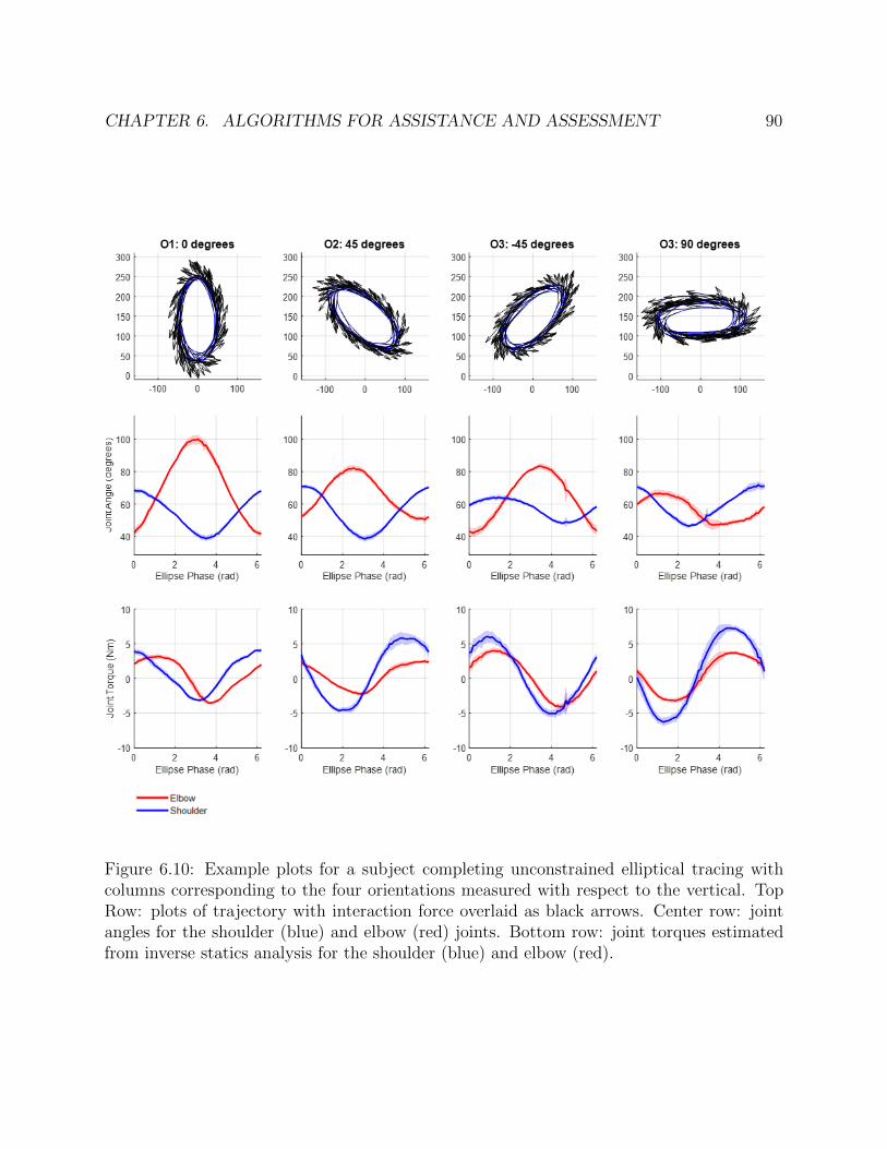
CHAPTER 6. ALGORITHMS FOR ASSISTANCE AND ASSESSMENT 90
Figure 6.10: Example plots for a subject completing unconstrained elliptical tracing withcolumns corresponding to the four orientations measured with respect to the vertical. TopRow: plots of trajectory with interaction force overlaid as black arrows. Center row: jointangles for the shoulder (blue) and elbow (red) joints. Bottom row: joint torques estimatedfrom inverse statics analysis for the shoulder (blue) and elbow (red).
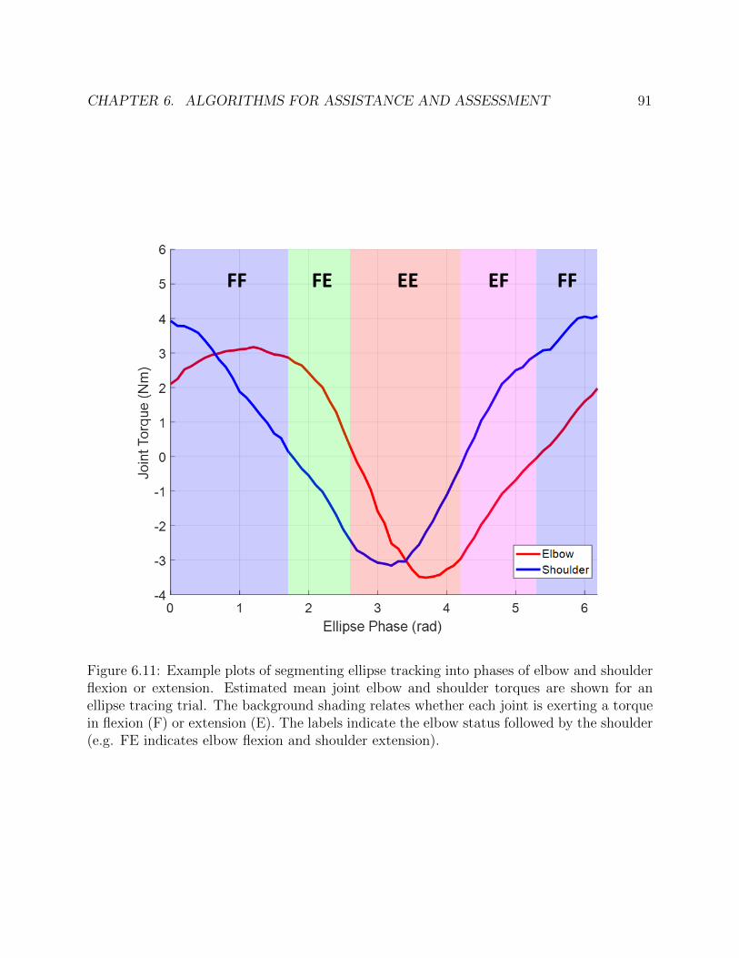
CHAPTER 6. ALGORITHMS FOR ASSISTANCE AND ASSESSMENT 91
Figure 6.11: Example plots of segmenting ellipse tracking into phases of elbow and shoulderflexion or extension. Estimated mean joint elbow and shoulder torques are shown for anellipse tracing trial. The background shading relates whether each joint is exerting a torquein flexion (F) or extension (E). The labels indicate the elbow status followed by the shoulder(e.g. FE indicates elbow flexion and shoulder extension).
CHAPTER 6. ALGORITHMS FOR ASSISTANCE AND ASSESSMENT 92
This static analysis neglects forces due to the arm dynamics. For faster motions, thismay result in inaccuracies in the computed joint torque. However, the force due to theacceleration of the mass of the limb segments is relatively small compared to the exertedend-effector forces. We additionally assume that the movement at the shoulder is confinedto the glenohumeral joint, with no movement of the scapula or torso.
Figure 6.10 shows example plots of end-effectors forces, estimated joint angles, and esti-mated joint torques for each orientation. As noted, there were no significant differences inthe selected end-effector-based metrics presented in Section 6.4. As intended, we do observedifferences in the joint range of motion and joint torques for the different orientations. Forexample, consider orientation 1 (O1) with semi-major axis aligned with the vertical andorientation 4 (O4) with semi-major axis aligned with the horizontal. The range of motionfor the elbow joint is much greater in O1 than O4. The joint angles will be different forreach subjects as they depend on the subjects limb lengths.
From the estimated joint torques, it is straightforward to segment each ellipse trajectoryinto times in which each joint producing a flexion or extension torque 6.11. This analysisis useful because it allows for a combination of isometric and eccentric/concentric testing offunction as part of a higher level task. Additionally, this provides a first step toward designingprotocols which target specific deficits at the joint-level or involving joint synergies. Futurework can explore incorporating this into the selection of desired trajectories.
6.5 Strength Assessment via Joint Motion Isolation
In this section, we present a framework for the assessment of joint strength and coordinationby constraining the end-effector to isolate the motion of a single joint. While it is possibleto attain kinematic isolation of the shoulder or elbow motion, we note that this does notcorrespond to isolating the joint torque. In order to produce an end-effector force tangentto the motion, the immobile joint must produce a torque to balance the torque producedby the joint in motion. Resolving the joint torques from the measured end-effector forces,we can gain insight into the elbow strength, shoulder strength, and joint coordination. Theinitial feasibility is demonstrated on a single healthy control subject.
Methodology
An illustration of the proposed method for joint isolation is shown in 6.12. For this section,we assume the device is operating at shoulder height and model the arm as a two-joint planarlinkage. To isolate the motion of the elbow and shoulder joints, we must know the location ofthe joint center. This can be accomplished by manual measurement (with a ruler) or throughvisual sensing with a top mounted camera or motion capture system. We can alternativelyestimate the joint center from device data alone by performing a calibration procedure withthe device to estimate the joint centers through a functional recovery method. With thedevice under an unconstrained admittance controller, the subject can complete isolated joint

CHAPTER 6. ALGORITHMS FOR ASSISTANCE AND ASSESSMENT 93
Figure 6.12: Illustration of the joint motion isolation protocol with elbow isolation on theleft and shoulder isolation on the right.
Figure 6.13: Visualization of the motion capture data from the joint isolation trials of theelbow joint (left) and shoulder joint (right).

CHAPTER 6. ALGORITHMS FOR ASSISTANCE AND ASSESSMENT 94
motions. In the case of a subject with limited ability to complete these isolated motions, thetherapist or researcher can guide the arm through these motions. From the position data,we can compute the best fit joint center location.
During the joint isolation protocol, we enforce a circular trajectory, centered at thepredetermined joint center. We set a hard constraint which locks the end-effector onto thetarget trajectory. To implement this, we set our virtual admittance dynamics to have novelocity response along the direction normal to the trajectory (an infinitely stiff spring).The viscosity is set such that there is no carry-over velocity from the previous timestep. Toincrease the strength required to complete the motion, we make the task more difficult bysetting the virtual mass of the admittance control to be high. For the preliminary test, themass was set to be 16 kg. This value can be adjusted for each individual. In future work, wecan expand this by having the mass parameter adjusted in real-time to optimally challengethe subject. Beginning at a fully flexed position, the subject will extend their joint throughtheir full range of motion. This will measure the subjects ability to generate joint torquethrough a continuous range of joint angles. In the case of a subject with a high level ofspasticity and contracture and decreased ability to produce an active joint torque (such asthe case for some patients with spinal cord injury), the device can be used to measure thepassive stiffness of the arm by moving the subject. This can also be used to identify thepassive range of motion.
For this experiment, a passive support was attached to provide gravity compensation forthe arm. The device, modified from the Wilmington Robotics Exoskeleton [111], supportsthe arm just above the elbow. The subject’s left arm was otherwise connected to the deviceas described in Section 6.3. Motion capture markers were used to track the motion of thehuman and device. The subject, a healthy young adult female, completed trials consisting ofthree extension-flexion motions, in which she moved from a fully flexed to a fully extendedposition with a small pause after each completed motion. The elbow was tested with theshoulder at 90 degrees, extended forward in front of the subject. The shoulder was testedwith the elbow flexed at approximately 115 degrees.
Results
To demonstrate feasibility of the method, we first show that the device successfully isolatedthe motion of the joint. Motion capture data was collected to validate the motion of thearm during the joint isolation trials. Figure 6.13 shows traces of the motion capture markersduring elbow and shoulder isolation trials. We observe the task space motion along a circulararc corresponding to motion of a single joint. We expect the joint center to remain stationaryduring the single joint motion. There is, however, some translation of the joint center ofinterest in both the shoulder and elbow isolation. Several factors may contribute to thiserror. First, the approximate joint center was marked by a single motion capture marker.For the elbow joint, especially, the position of this marker will be effected by skin motionartifact due to the changing shape of the muscle belly. We expect this to less pronouncedfor the shoulder joint, whose motion may be due to error in the selection of the joint center

CHAPTER 6. ALGORITHMS FOR ASSISTANCE AND ASSESSMENT 95
Figure 6.14: Example plots of the end effector forces measured during the joint isolationprotocol for flexion and extension of the elbow and shoulder joints.
or the presence of scapular motion during the motion. Additional error may result from thesubject moving their torso during the trial.
Examples of the recorded end-effector forces are shown in figure 6.14. The direction ofthe force is primarily tangent to the joint isolation trajectory, indicating that the subjectwas able to regulate the combination of the shoulder and elbow torques to generate anend-effector force in the correct direction. Joint torques were recovered using the inversestatic analysis method described in Section 6.4. The resultant net joint torques for an elbowisolation trial and a shoulder isolation trial are shown in Figure 6.15. The torque across thethree trials was averaged by joint angle with the standard deviation at each point denotedby the shaded region around the mean. We observe good repeatability between the motionsas evidenced by the size of the shaded region. For the elbow isolation trials, we observe anearly constant joint torque of 6 Nm in elbow extension and 5 Nm in elbow flexion. Tocounterbalance the constant elbow torque, we observe that the shoulder torque must varywith elbow angle. The shoulder must initially produce an extension torque which variesto then produce a flexion torque. In the case of isolated shoulder motion, the elbow jointmust produce a torque in the same direction as the shoulder. The shoulder joint torques

CHAPTER 6. ALGORITHMS FOR ASSISTANCE AND ASSESSMENT 96
Figure 6.15: Estimated joint torques for shoulder (blue) and elbow (red) joints during elbowisolation (left) and shoulder isolation (right). Each plot shows the mean for three trials withthe standard deviation shaded.
were relatively constant at approximately 10 Nm in both extension and flexion. In a subjectwith deficits in strength or coordination, we would expect to see these manifest in the peakjoint torques or the inability to coordinate the joint torque to produce an end effector forcetangent to the isolated motion trajectory.
6.6 Chapter Summary
In this chapter, we presented two protocols for robot-assisted assessment using the robotictherapy device described in Chapter 5. These control strategies expand upon the admittancecontrol framework, incorporating assistive force fields and hard constraints.
In the first method, we add a spring term into the virtual dynamics model, providing arestoring force in the direction normal to the trajectory. We demonstrate the ability of ourlow-cost system to produce force fields on curved trajectories. Human subject experimentsstudied the phenomenon of subject reliance on assistance. The results support the hypothesisthat subjects will exploit the assistive force field and lean in to the force field to achievea smoother motion. While previous work has found that humans slack to minimize theenergy of the motion, we found that the assistance resulted in greater exertion as evidencedby greater total force and force in the correct direction. These findings can inform the

CHAPTER 6. ALGORITHMS FOR ASSISTANCE AND ASSESSMENT 97
design of robotic rehabilitation therapy protocols for subjects with coordination deficits. Byeliminating the need to produce an end-effector first in a precise direction, assistive forcefields can encourage rehabilitiative exercise with greater force output and faster motion.
The second method presents a protocol for assessment of strength and joint coordinationthrough isolated joint motions, enabling measurement through a continuous range of jointangles. Through the implementation of constraints, we can decompose the strength ateach joint with the coordination required to complete the motion. Initial feasibility wasdemonstrated through results on a single healthy control subject.
98
Chapter 7
Final Thoughts and Future Work
In this dissertation, we explored methods for assessing and assisting human motion with theaim of developing clinically accessible technologies. Our approach integrated biomechanicalmodeling into the design and development of affordable hardware systems and the accom-panying analysis methods. We placed a large emphasis on experimental validation throughboth hardware characterization and human subjects experiments.
We first presented a framework for improved kinematic recovery by imposing a rigid-body model on noisy data from a single depth camera. A validation study comparing thealgorithm to a marker-based motion capture system demonstrated the feasibility of thesystem to be used as an accurate and fast tool for human motion analysis in clinic. Thisframework has since been utilized in additional work outside of the scope of this thesis.Building on the kinematic recovery, a dynamic model was integrated and validated [112].This work estimated joint torques and back loading computed through inverse dynamicsanalysis using the recovered kinematics. Ongoing and future work using this technology willcontinue with our clinical collaborators who can utilize the tool for motion analysis studiesin patient populations. These methods have been applied to a longitudinal study of a cohortof subjects with adult spinal deformity completing sit-to-stand (STS) [113] and are currentlybeing used as a standard measure in the National Institute of Health REACH Initiative forunderstanding low-back pain.
Secondly, we introduced a simple passive device which provides bilateral knee assistanceduring STS. Our preliminary results indicated both the ability to aid in completing the mo-tion by reducing the required human knee torque and the potential to encourage desirablechanges in whole-body motion. A number of future directions would expand on these initialexperiments. First, an electromyography (EMG) study could be used to better understandhow the device and changes in overall strategy affect muscle activity and recruitment. Ad-ditionally, the effects of the device should be tested on a larger cohort as well as a clinicalcohort. We note that the device was not developed for daily assistance and significant modi-fications, including the development of a clutch mechanism to disengage the elastic element,would need to be incorporated to allow for daily use. In its current form, the device is moresuited to rehabilitation protocols.

CHAPTER 7. FINAL THOUGHTS AND FUTURE WORK 99
Finally, we introduced an affordable upper limb planar robotic manipulandum. Humansubjects studies demonstrated the feasibility of the device to be used for robot-assisted assess-ment and therapy. Building on the admittance control framework, we proposed a numberof extensions which were not fully explored in this dissertation, including the integrationof a muscle model and a method for the assessment of joint-level range of motion, pas-sive stiffness, and strength through isolated joint motions. In combination with task-spacerehabilitation protocols, the joint isolation method has the potential provide decipherableinformation on the underlying limitations behind functional deficits. This information canbe used to inform subject-specific models of impairment which in turn can determine optimalprotocols for robot-assisted rehabilitation and assistance. These case studies would greatlybenefit from formalized experiments on a larger cohort of patients with upper limb impair-ment. This is the only way to truly demonstrate the efficacy of the device. Our design hasbeen replicated by our collaborators at Hong Kong University of Science and Technology aswell as University of California, San Francisco, for the development of eye-gaze and brain-computer interfaces. Through the development of this low-cost device, we hope to expandthe accessibility of robotic platforms for incorporation in clinical care and research studies.

100
Bibliography
[1] Michelle E. Mlinac and Michelle C. Feng. “Assessment of Activities of Daily Living,Self-Care, and Independence”. In: Archives of Clinical Neuropsychology (2016). issn:08876177. doi: 10.1093/arclin/acw049.
[2] Robert Peter Matthew et al. “Kinematic and Kinetic Validation of an ImprovedDepth Camera Motion Assessment System Using Rigid Bodies”. In: IEEE Journalof Biomedical and Health Informatics (2019). issn: 21682208. doi: 10.1109/JBHI.2018.2872834.
[3] Sarah Seko et al. “A functional method for generating individualized spine mod-els from motion-capture data”. In: Proceedings of the Annual International Confer-ence of the IEEE Engineering in Medicine and Biology Society, EMBS. 2018. isbn:9781538636466. doi: 10.1109/EMBC.2018.8512580.
[4] Sarah Seko et al. “Passive Knee Assistance Affects Whole-Body Biomechanics duringSit-to-Stand”. In: Proceedings of the Annual International Conference of the IEEEEngineering in Medicine and Biology Society, EMBS. 2019. isbn: 9781538613115.doi: 10.1109/EMBC.2019.8856477.
[5] William Thomas Crow and David R. Willis. “Estimating cost of care for patients withacute low back pain: a retrospective review of patient records.” eng. In: The Journalof the American Osteopathic Association 109.4 (2009), pp. 229–33. issn: 1945-1997.doi: 10.7556/jaoa.2009.109.4.229.
[6] Andre J Cardin and Camille Hadida. “Evaluation of lumbar intersegmental rangeof motion using flexion-extension radiographs of asymptomatic versus low back painadults”. In: The Journal of the Canadian Chiropractic Association 38.2 (June 1994),pp. 83–89. issn: 0008-3194.
[7] Balkan Cakir et al. “Evaluation of lumbar spine motion with dynamic X-ray–a reli-ability analysis.” eng. In: Spine 31.11 (May 2006), pp. 1258–1264. issn: 0362-2436.doi: 10.1097/01.brs.0000217763.80593.50.
[8] B. J. Van Royen et al. “Accuracy of the sagittal vertical axis in a standing lateralradiograph as a measurement of balance in spinal deformities”. In: European SpineJournal 7.5 (1998), pp. 408–412. issn: 09406719. doi: 10.1007/s005860050098.

BIBLIOGRAPHY 101
[9] S. S. Coghlin and B. J. McFadyen. “Transfer strategies used to rise from a chair innormal and low back pain subjects”. In: Clinical Biomechanics 9.2 (1994), pp. 85–92.issn: 02680033. doi: 10.1016/0268-0033(94)90029-9.
[10] Elisabetta Papa and Aurelio Cappozzo. “Sit-to-stand motor strategies investigatedin able-bodied young and elderly subjects”. In: Journal of Biomechanics 33.9 (2000),pp. 1113–1122. issn: 00219290. doi: 10.1016/S0021-9290(00)00046-4.
[11] Stephanie L. Jones et al. “Individuals with non-specific low back pain use a trunkstiffening strategy to maintain upright posture”. In: Journal of Electromyography andKinesiology 22.1 (2012), pp. 13–20. issn: 10506411. doi: 10.1016/j.jelekin.2011.10.006.
[12] John Rasmussen et al. “The anybody project – computer analysis of the humanbody”. In: Biomechanics of Man (2002), pp. 270–274.
[13] Scott L Delp et al. “OpenSim: Open source to create and analyze dynamic simula-tions of movement”. In: IEEE transactions on bio-medical engineering 54.11 (2007),pp. 1940–1950. issn: 0018-9294. doi: 10.1109/TBME.2007.901024. arXiv: 15334406.
[14] W. S. Marras et al. “Accuracy of a three-dimensional lumbar motion monitor forrecording dynamic trunk motion characteristics”. In: International Journal of Indus-trial Ergonomics 9.1 (1992), pp. 75–87.
[15] Sue A. Ferguson, William S. Marras, and Purnendu Gupta. “Longitudinal quantita-tive measures of the natural course of low back pain recovery”. In: Spine 25.15 (2000),pp. 1950–1956. issn: 03622436. doi: 10.1097/00007632-200008010-00014.
[16] William R. Taylor, Tobias Consmuller, and Antonius Rohlmann. “A novel system forthe dynamic assessment of back shape”. In: Medical Engineering and Physics 32.9(2010), pp. 1080–1083. issn: 13504533. doi: 10.1016/j.medengphy.2010.07.011.
[17] Tobias Consmuller et al. “Comparative evaluation of a novel measurement tool toassess lumbar spine posture and range of motion.” In: European spine journal : officialpublication of the European Spine Society, the European Spinal Deformity Society, andthe European Section of the Cervical Spine Research Society 21.11 (2012), pp. 2170–80. issn: 1432-0932. doi: 10.1007/s00586-012-2312-1.
[18] Zhengyou Zhang. “Microsoft Kinect sensor and its effect”. In: IEEE Multimedia 19.2(2012), pp. 4–10. issn: 1070986X. doi: 10.1109/MMUL.2012.24.
[19] Alexandra Pfister et al. “Comparative abilities of Microsoft Kinect and Vicon 3Dmotion capture for gait analysis”. In: Journal of Medical Engineering and Technology38.5 (2014), pp. 274–280. issn: 1464522X. doi: 10.3109/03091902.2014.909540.
[20] Julia K. Nichols et al. “A Kinect-based movement assessment system: marker posi-tion comparison to Vicon”. In: Computer Methods in Biomechanics and BiomedicalEngineering 20.12 (2017), pp. 1289–1298. issn: 14768259. doi: 10.1080/10255842.2017.1340464.

BIBLIOGRAPHY 102
[21] Catalin Ionescu et al. “Human3.6M: Large scale datasets and predictive methodsfor 3D human sensing in natural environments”. In: IEEE Transactions on PatternAnalysis and Machine Intelligence 36.7 (2014), pp. 1325–1339. issn: 01628828. doi:10.1109/TPAMI.2013.248.
[22] Georgios Pavlakos et al. “Coarse-to-fine volumetric prediction for single-image 3D hu-man pose”. In: Proceedings - 30th IEEE Conference on Computer Vision and PatternRecognition, CVPR 2017 2017-Janua (2017), pp. 1263–1272. doi: 10.1109/CVPR.2017.139. arXiv: 1611.07828.
[23] Sungheon Park, Jihye Hwang, and Nojun Kwak. “3D Human Pose Estimation UsingConvolutional Neural Networks with 2D Pose Information”. In: European Conferenceon Computer Vision (ECCV) Workshop. 2016, pp. 156–169. isbn: 9783319494081.doi: 10.1007/978-3-319-49409-8_15. arXiv: 1608.03075.
[24] Xingyi Zhou et al. “Deep kinematic pose regression”. In: European Conference onComputer Vision. 2016, pp. 186–201. isbn: 9783319494081. doi: 10.1007/978-3-319-49409-8_17. arXiv: 1609.05317.
[25] Dushyant Mehta et al. “VNect: Real-time 3D Human Pose Estimation with a Sin-gle RGB Camera”. In: ACM Transactions on Graphics 36.4 (2017), pp. 1–14. issn:15577368. doi: 10.1145/3072959.3073596. arXiv: 1705.01583.
[26] Carsten Stoll et al. “Fast articulated motion tracking using a sums of Gaussians bodymodel”. In: Proceedings of the IEEE International Conference on Computer Vision.2011, pp. 951–958. isbn: 9781457711015. doi: 10.1109/ICCV.2011.6126338.
[27] Meng Ding and Guoliang Fan. “Articulated and generalized Gaussian kernel corre-lation for human pose estimation”. In: IEEE Transactions on Image Processing 25.2(2016), pp. 776–789. issn: 10577149. doi: 10.1109/TIP.2015.2507445.
[28] Liang Shuai et al. “Motion Capture with Ellipsoidal Skeleton Using Multiple DepthCameras”. In: IEEE Transactions on Visualization and Computer Graphics 23.2(2017), pp. 1085–1098. issn: 10772626. doi: 10.1109/TVCG.2016.2520926.
[29] NASA. “Anthropometric Source Book Volume I: Anthropometry for Designers”. In:I.2 (1978), pp. 1–606. issn: 0717-6163. doi: 10.1007/s13398-014-0173-7.2. arXiv:9809069v1 [arXiv:gr-qc].
[30] Don B Chaffin. “Development of Computerized Human Static Strength SimulationModel for Job Design”. In: Human Factors and Ergonomics in Manufacturing 7.4(1997), pp. 305–322. issn: 1090-8471. doi: 10.1002/(SICI)1520-6564(199723)7:43.3.CO;2-S.
[31] Don B. Chaffin, Gunnar B. J. Andersson, and Bernard J. Martin. Occupational Biome-chanics. 4th. New York: John Wiley & Sons. isbn: 0-471-24697-2.
[32] Scott L. Delp and J. Peter Loan. “A graphics-based software system to develop andanalyze models of musculoskeletal structures”. In: Computers in Biology and Medicine25.1 (1995), pp. 21–34. issn: 00104825. doi: 10.1016/0010-4825(95)98882-E.

BIBLIOGRAPHY 103
[33] Mohammad Ali Rajaee et al. “Comparative evaluation of six quantitative lifting toolsto estimate spine loads during static activities”. In: Applied Ergonomics 48 (2015),pp. 22–32. issn: 18729126. doi: 10.1016/j.apergo.2014.11.002.
[34] Kevin M Lynch and Frank C Park. Modern Robotics: Mechanics, Planning, and Con-trol. Cambridge University Press, 2017.
[35] Ko Ayusawa, Gentiane Venture, and Yoshihiko Nakamura. “Identification of hu-manoid robots dynamics using floating-base motion dynamics”. In: 2008 IEEE/RSJInternational Conference on Intelligent Robots and Systems, IROS (2008), pp. 2854–2859. doi: 10.1109/IROS.2008.4650614.
[36] Johannes Buckup. Clinical tests for the musculoskeletal system: examinations-signs-phenomena. TPS, 2016.
[37] Don B. Chaffin, Gunnar B. J. Andersson, and Bernard J. Martin. Occupational Biome-chanics. 1999.
[38] Simon J. Julier and Jeffrey K. Uhlmann. “New extension of the Kalman filter tononlinear systems”. In: July 1997 (1997), p. 182. issn: 0277786X. doi: 10.1117/12.280797.
[39] E. A. Wan and R. Van Der Merwe. “The unscented Kalman filter for nonlinear es-timation”. In: IEEE 2000 Adaptive Systems for Signal Processing, Communications,and Control Symposium, AS-SPCC 2000 February 2000 (2000), pp. 153–158. issn:15270297. doi: 10.1109/ASSPCC.2000.882463.
[40] Matthew Reed, Miriam A. Manary, and Lawrence W. Schneider. “Methods for Mea-suring and Representing Automobile Occupant Posture”. In: 724 (1999). issn: 0148-7191. doi: 10.4271/1999-01-0959.
[41] Charles K. Anderson, Don B. Chaffin, and Gary D. Herrin. “A study of lumbosacralorientation under varied static loads”. In: Spine 11.5 (1986), pp. 456–462. issn:15281159. doi: 10.1097/00007632-198606000-00012.
[42] H.M. Reynolds, C.C. Snow, and J.W. Young. Spatial Geometry of the Human Pelvis.Oklahoma City, OK, 1982.
[43] Vicon®. “Plug-in-Gait Marker Placement”. In: Mocap (2006).
[44] Ge Wu et al. “ISB recommendation on definitions of joint coordinate system of variousjoints for the reporting of human joint motion—part I: ankle, hip, and spine”. In:Journal of Biomechanics 35.4 (2002), pp. 543–548. issn: 00219290. doi: 10.1016/S0021-9290(01)00222-6. arXiv: 44.
[45] Hans Kainz et al. “Reliability of functional and predictive methods to estimate thehip joint centre in human motion analysis in healthy adults”. In: Gait and Posture53 (2017), pp. 179–184. issn: 18792219. doi: 10.1016/j.gaitpost.2017.01.023.

BIBLIOGRAPHY 104
[46] Thor F. Besier et al. “Repeatability of gait data using a functional hip joint centreand a mean helical knee axis”. In: Journal of Biomechanics 36.8 (2003), pp. 1159–1168. issn: 00219290. doi: 10.1016/S0021-9290(03)00087-3.
[47] Margaret K.Y. Mak et al. “Joint torques during sit-to-stand in healthy subjects andpeople with Parkinson’s disease”. In: Clinical Biomechanics 18.3 (2003), pp. 197–206.issn: 02680033. doi: 10.1016/S0268-0033(02)00191-2.
[48] Josip Music, Roman Kamnik, and Marko Munih. “Model based inertial sensing ofhuman body motion kinematics in sit-to-stand movement”. In: Simulation ModellingPractice and Theory 16.8 (2008), pp. 933–944. issn: 1569190X. doi: 10.1016/j.simpat.2008.05.005.
[49] L I Lin et al. “A proposal for strength-of-agreement criteria for Lin’s ConcordanceCorrelation Coefficient”. In: NIWA Client Report 45.1 (2005), pp. 307–310. issn:0006-341X. doi: 10.2307/2532051.
[50] P E Shrout and J L Fleiss. “Intraclass correlations-uses in assessing rater reliability”.In: Psychological Bulletin 86.2 (1979), pp. 420–428. doi: 10.1037//0033-2909.86.2.420.
[51] Kenneth O. McGraw and S. P. Wong. “Forming Inferences about Some Intraclass Cor-relation Coefficients”. In: Psychological Methods 1.1 (1996), pp. 30–46. issn: 1082989X.doi: 10.1037/1082-989X.1.1.30.
[52] Terry K. Koo and Mae Y. Li. “A Guideline of Selecting and Reporting Intraclass Cor-relation Coefficients for Reliability Research”. In: Journal of Chiropractic Medicine15.2 (2016), pp. 155–163. issn: 15563707. doi: 10.1016/j.jcm.2016.02.012. arXiv:PMC4913118.
[53] Domenic V. Cicchetti. “Guidlines, Criteria, and Rules of Thumb for EvalautingNormed and Standardized Assessment Instruments in Psychology”. In: Psycholog-ical Assessment 6.4 (1994), pp. 284–290. issn: 1939-134X. doi: 10.1037/1040-
3590.6.4.284.
[54] Moataz Eltoukhy et al. “Validation of Static and Dynamic Balance Assessment usingMicrosoft Kinect for Young and Elderly Populations”. In: IEEE Journal of Biomedicaland Health Informatics (2017), pp. 1–1. issn: 2168-2194. doi: 10.1109/JBHI.2017.2686330.
[55] Ferda Ofli, Rizwan Chaudhry, and Gregorij Kurillo. “Berkeley Multimodal HumanAction Database (MHAD)”. In: (2014).
[56] Q. Wang et al. “Smart Rehabilitation Garment for posture monitoring”. In: Proceed-ings of the Annual International Conference of the IEEE Engineering in Medicineand Biology Society, EMBS 2015-Novem (2015), pp. 5736–5739. issn: 1557170X. doi:10.1109/EMBC.2015.7319695.
BIBLIOGRAPHY 105
[57] R. J. Full and D. E. Koditschek. “Templates and anchors: Neuromechanical hypothe-ses of legged locomotion on land”. In: Journal of Experimental Biology (1999). issn:00220949.
[58] Richard G. Snyder, Don B. Chaffin, and Rodney K. Schutz. Link System of the HumanTorso. Tech. rep. August 1972. Aerospace Medical Research Laboratory.
[59] D. H. Robbins. Anthropometric Specificaitons for Mid-Sized Male Dummy, Voume 2.Tech. rep. The UNiversity of Michigan, Transportation Research Institute, 1983.
[60] Alberto Leardini et al. “Validation of a functional method for the estimation of hipjoint centre location”. In: Journal of Biomechanics (1999). issn: 00219290. doi: 10.1016/S0021-9290(98)00148-1.
[61] Oliver Rettig et al. “A new kinematic model of the upper extremity based on func-tional joint parameter determination for shoulder and elbow”. In: Gait and Posture(2009). issn: 09666362. doi: 10.1016/j.gaitpost.2009.07.111.
[62] K. Han Kim et al. “Adaptation of torso movement strategies in persons with spinalcord injury or low back pain”. In: Spine (2010). issn: 03622436. doi: 10.1097/BRS.0b013e3181cb4769.
[63] Maarten F. Bobbert et al. “Searching for strategies to reduce the mechanical demandsof the sit-to-stand task with a muscle-actuated optimal control model”. In: ClinicalBiomechanics (2016). issn: 18791271. doi: 10.1016/j.clinbiomech.2016.06.008.
[64] Charles K. Anderson et al. “A biomechanical model of the lumbosacral joint duringlifting activities”. In: Journal of Biomechanics (1985). issn: 00219290. doi: 10.1016/0021-9290(85)90012-0.
[65] A. Nerot, W. Skalli, and X. Wang. “Estimation of spinal joint centers from externalback profile and anatomical landmarks”. In: Journal of Biomechanics (2018). issn:18732380. doi: 10.1016/j.jbiomech.2017.11.013.
[66] Ge Wu et al. “ISB recommendation on definitions of joint coordinate systems ofvarious joints for the reporting of human joint motion - Part II: Shoulder, elbow,wrist and hand”. In: Journal of Biomechanics (2005). issn: 00219290. doi: 10.1016/j.jbiomech.2004.05.042.
[67] Richard M. Murray, Zexiang Li, and S. Shankar Sastry. A mathematical introduc-tion to robotic manipulation. CRC Press, 1994. isbn: 9781351469791. doi: 10.1201/9781315136370.
[68] D H Robbins. Anthropometric Specifications for Small Female and Large Male Dum-mies - Volume 3. 1983.
[69] Patrick O. Riley et al. “Mechanics of a constrained chair-rise”. In: Journal of Biome-chanics (1991). issn: 00219290. doi: 10.1016/0021-9290(91)90328-K.
BIBLIOGRAPHY 106
[70] P. O. Riley, D. E. Krebs, and R. A. Popat. “Biomechanical analysis of failed sit-to-stand”. In: IEEE Transactions on Rehabilitation Engineering (1997). issn: 10636528.doi: 10.1109/86.650289.
[71] M. A. Hughes et al. “Chair rise strategies in the elderly”. In: Clinical Biomechanics(1994). issn: 02680033. doi: 10.1016/0268-0033(94)90020-5.
[72] Gary L.K. Shum, Jack Crosbie, and Raymond Y.W. Lee. “Effect of low back painon the kinematics and joint coordination of the lumbar spine and hip during sit-to-stand and stand-to-sit”. In: Spine (2005). issn: 03622436. doi: 10.1097/01.brs.0000176195.16128.27.
[73] Bing Chen et al. Knee exoskeletons for gait rehabilitation and human performanceaugmentation: A state-of-the-art. 2019. doi: 10.1016/j.mechmachtheory.2019.01.016.
[74] Nikos Karavas et al. “Tele-impedance based assistive control for a compliant kneeexoskeleton”. In: Robotics and Autonomous Systems. 2015. doi: 10.1016/j.robot.2014.09.027.
[75] Max K. Shepherd and Elliott J. Rouse. “Design and Validation of a Torque-ControllableKnee Exoskeleton for Sit-to-Stand Assistance”. In: IEEE/ASME Transactions onMechatronics (2017). issn: 10834435. doi: 10.1109/TMECH.2017.2704521.
[76] Bing Chen et al. “Sit-to-stand and stand-to-sit assistance for paraplegic patientswith CUHK-EXO exoskeleton”. In: Robotica (2018). issn: 14698668. doi: 10.1017/S0263574717000546.
[77] Stuart Diller, Carmel Majidi, and Steven H. Collins. “A lightweight, low-power elec-troadhesive clutch and spring for exoskeleton actuation”. In: Proceedings - IEEE In-ternational Conference on Robotics and Automation. 2016. isbn: 9781467380263. doi:10.1109/ICRA.2016.7487194.
[78] Daisuke Kaneishi, Robert Peter Matthew, and Masayoshi Tomizuka. “Optimal Con-trol Parameterization for ActivelPassive EXoskeleton with Variable Impedance Ac-tuator”. In: Proceedings of the IEEE RAS and EMBS International Conference onBiomedical Robotics and Biomechatronics. 2018. isbn: 9781538681831. doi: 10.1109/BIOROB.2018.8487719.
[79] Daisuke Kaneishi, Masayoshi Tomizuka, and Robert Peter Matthew. “Characteriza-tion of Active/Passive Pneumatic Actuators for Assistive Devices”. In: IEEE Inter-national Conference on Intelligent Robots and Systems. 2018. isbn: 9781538680940.doi: 10.1109/IROS.2018.8594143.
[80] Kamran Shamaei et al. “Design and evaluation of a quasi-passive knee exoskeletonfor investigation of motor adaptation in lower extremity joints”. In: IEEE Transac-tions on Biomedical Engineering (2014). issn: 15582531. doi: 10.1109/TBME.2014.2307698.

BIBLIOGRAPHY 107
[81] Kamran Shamaei et al. “Biomechanical effects of stiffness in parallel with the kneejoint during walking”. In: IEEE Transactions on Biomedical Engineering (2015). issn:15582531. doi: 10.1109/TBME.2015.2428636.
[82] Steven H. Collins, M. Bruce Wiggin, and Gregory S. Sawicki. “Reducing the energycost of human walking using an unpowered exoskeleton”. In: Nature (2015). issn:14764687. doi: 10.1038/nature14288.
[83] F. C. Park, J. E. Bobrow, and S. R. Ploen. “A Lie Group Formulation of Robot Dy-namics”. In: The International Journal of Robotics Research (1995). issn: 17413176.doi: 10.1177/027836499501400606.
[84] H. I. Krebs et al. “Rehabilitation robotics: Performance-based progressive robot-assisted therapy”. In: Autonomous Robots 15.1 (2003), pp. 7–20. issn: 09295593.doi: 10.1023/A:1024494031121.
[85] Tobias Nef, Marco Guidali, and Robert Riener. “ARMin III – Arm Therapy Exoskele-ton with an Ergonomic Shoulder Actuation”. In: Applied Bionics and Biomechanics(2009). issn: 1176-2322. doi: 10.1155/2009/962956.
[86] Domenico Campolo et al. “H-Man: A planar, H-shape cabled differential robotic ma-nipulandum for experiments on human motor control”. In: Journal of NeuroscienceMethods 235 (2014), pp. 285–297. issn: 1872678X. doi: 10.1016/j.jneumeth.2014.07.003.
[87] Giulio Rosati, Paolo Gallina, and Stefano Masiero. “Design, implementation and clin-ical tests of a wire-based robot for neurorehabilitation”. In: IEEE Transactions onNeural Systems and Rehabilitation Engineering (2007). issn: 15344320. doi: 10 .
1109/TNSRE.2007.908560.
[88] Robert Riener, T. Nef, and G. Colombo. “Robot-aided neurorehabilitation of the up-per extremities”. In: Medical and Biological Engineering and Computing 43.1 (2005),pp. 2–10. issn: 01400118. doi: 10.1007/BF02345116.
[89] Carol L. Richards, Francine Malouin, and Sylvie Nadeau. Stroke rehabilitation: Clin-ical picture, assessment, and therapeutic challenge. 1st ed. Vol. 218. Elsevier B.V.,2015, pp. 253–280. doi: 10.1016/bs.pbr.2015.01.003.
[90] Angelo Basteris et al. Training modalities in robot-mediated upper limb rehabilitationin stroke: A framework for classification based on a systematic review. 2014. doi:10.1186/1743-0003-11-111.
[91] Alexander Duschau-wicke et al. “Haptic Constraints for Rehabilitation Robots : AnOverview Haptic Constraints”. In: Biomed Tech. Vol. 55. 2010. doi: 10.1515/BMT.2010.481.
[92] Rui C.V. Loureiro and William S. Harwin. “Reach & grasp therapy: Design andcontrol of a 9-DOF robotic neuro-rehabilitation system”. In: 2007 IEEE 10th Inter-national Conference on Rehabilitation Robotics, ICORR’07 00.c (2007), pp. 757–763.doi: 10.1109/ICORR.2007.4428510.
BIBLIOGRAPHY 108
[93] Laura Marchal-Crespo and David J. Reinkensmeyer. “Review of control strategies forrobotic movement training after neurologic injury”. In: Journal of NeuroEngineeringand Rehabilitation 6.1 (2009). issn: 17430003. doi: 10.1186/1743-0003-6-20.
[94] M. P. Dijkers et al. “Patient and staff acceptance of robotic technology in occupationaltherapy: A pilot study”. In: Journal of Rehabilitation Research and Development(1991). issn: 0007506X. doi: 10.1682/jrrd.1991.04.0033.
[95] Pawe l Maciejasz et al. “A survey on robotic devices for upper limb rehabilitation”.In: Journal of NeuroEngineering and Rehabilitation 11.3 (2014). issn: 17430003. doi:10.1186/1743-0003-11-3.
[96] Arvid Q.L. Keemink, Herman van der Kooij, and Arno H.A. Stienen. “Admittancecontrol for physical human–robot interaction”. In: International Journal of RoboticsResearch 37.11 (2018), pp. 1421–1444. issn: 17413176. doi: 10.1177/0278364918768950.
[97] Neville Hogan. “Impedance control: An approach to manipulation: Part I-theory”. In:Journal of Dynamic Systems, Measurement and Control, Transactions of the ASME(1985). issn: 15289028. doi: 10.1115/1.3140702.
[98] T. Flash and N. Hogan. “The coordination of arm movements: An experimentallyconfirmed mathematical model”. In: Journal of Neuroscience 5.7 (1985), pp. 1688–1703. issn: 02706474. doi: 10.1523/jneurosci.05-07-01688.1985.
[99] Laura Dipietro et al. “Submovement changes characterize generalization of motorrecovery after stroke”. In: Cortex 45.3 (2009), pp. 318–324. issn: 00109452. doi:10.1016/j.cortex.2008.02.008.
[100] Sebastien Mateo et al. “Upper limb kinematics after cervical spinal cord injury:A review”. In: Journal of NeuroEngineering and Rehabilitation 12.9 (2015). issn:17430003. doi: 10.1186/1743-0003-12-9.
[101] Evert Jan Nijhof and David A. Gabriel. “Maximum isometric arm forces in the hori-zontal plane”. In: Journal of Biomechanics (2006). issn: 00219290. doi: 10.1016/j.jbiomech.2005.01.004.
[102] Kenji Tahara et al. “Sensory-motor control mechanism for reaching movements ofa redundant musculo-skeletal arm”. In: Journal of Robotic Systems (2005). issn:07412223. doi: 10.1002/rob.20089.
[103] Matjaz Zadravec and Zlatko Matjacic. “Planar arm movement trajectory formation:An optimization based simulation study”. In: Biocybernetics and Biomedical Engi-neering (2013). issn: 02085216. doi: 10.1016/j.bbe.2013.03.006.
[104] F Amirabdollahian et al. Error correction movement for machine assisted stroke re-habilitation. Ed. by M Mokhtari. Amsterdam, The Netherlands: IOS Press, 2001,pp. 60–65. isbn: 1-58603-171-6.
BIBLIOGRAPHY 109
[105] David J. Reinkensmeyer et al. “Slacking by the human motor system: Computationalmodels and implic implications for robotic orthoses”. In: Proceedings of the 31st An-nual International Conference of the IEEE Engineering in Medicine and Biology Soci-ety: Engineering the Future of Biomedicine, EMBC 2009. 2009. isbn: 9781424432967.doi: 10.1109/IEMBS.2009.5333978.
[106] Urs Keller, Georg Rauter, and Robert Riener. “Assist-as-needed path control for thePASCAL rehabilitation robot”. In: IEEE International Conference on RehabilitationRobotics. 2013. isbn: 9781467360241. doi: 10.1109/ICORR.2013.6650475.
[107] Oliver M. O’Reilly. Engineering Dynamics: A Primer. Third Ed. New York: Spinger-Verlag, 2019. doi: 10.1007/978-3-030-11745-0.
[108] Francesco Lacquaniti, Carlo Terzuolo, and Paolo Viviani. “The law relating the kine-matic and figural aspects of drawing movements”. In: Acta Psychologica (1983). issn:00016918. doi: 10.1016/0001-6918(83)90027-6.
[109] Giovanna Catavitello et al. “Drawing ellipses in water: evidence for dynamic con-straints in the relation between velocity and path curvature”. In: Experimental BrainResearch 234.6 (2016), pp. 1649–1657. issn: 14321106. doi: 10.1007/s00221-016-4569-9.
[110] Pauline Maurice et al. “Velocity-Curvature Patterns Limit Human-Robot PhysicalInteraction”. In: IEEE Robotics and Automation Letters 3.1 (2018), pp. 249–256.issn: 23773766. doi: 10.1109/LRA.2017.2737048.
[111] Thierry Haumont et al. “Wilmington robotic exoskeleton: A novel device to maintainarm improvement in muscular disease”. In: Journal of Pediatric Orthopaedics 31.5(2011), pp. 44–49. issn: 02716798. doi: 10.1097/BPO.0b013e31821f50b5.
[112] Robert Peter Matthew et al. “Estimating Sit-to-Stand Dynamics Using a SingleDepth Camera”. In: IEEE Journal of Biomedical and Health Informatics (2019).issn: 21682208. doi: 10.1109/JBHI.2019.2897245.
[113] Jeannie F. Bailey et al. “ISSLS PRIZE IN BIOENGINEERING SCIENCE 2019:biomechanical changes in dynamic sagittal balance and lower limb compensatorystrategies following realignment surgery in adult spinal deformity patients”. In: Eu-ropean Spine Journal (2019). issn: 14320932. doi: 10.1007/s00586-019-05925-2.