robotic microphone arrays - washington university in st. louis

Robotic Microphone ArraysRobotic Microphone Arrays

Patricio S. La RosaPatricio S. La RosaCenter for Sensor Signal and Information Processing (CSSIP)Center for Sensor Signal and Information Processing (CSSIP)

Signal Processing Innovations in Research and Information TechnoSignal Processing Innovations in Research and Information Technologieslogies ((SPIRIT) LabSPIRIT) Lab

JanuaryJanuary 20102010

Department of Electrical & Systems Engineering

Faculty

Professor Arye

Nehorai

Research Associate

Ed Richter

PhD Students

Patricio S. La Rosa Phani

Chavali

Undergraduate Students

Chase LaFont, Evan Nixxon, Ian Beil, Raphael Schwartz, Zachary Knudsen

Former Students

Joshua York (BSEE09); Brian Blosser

(BSEE08), Matt Meshalum

(BSEE 09);

Tripp McGehee

(BSEE07)

AcknowledgmentsAcknowledgments

• Background

• Estimation Algorithms

• Control Algorithm

• Experimental Setup

• Demonstration

• Additional Modalities

• Conclusion

OverviewOverview

Goal: Modify microphone array configuration adaptively for improving the performance in estimating acoustic source position using generalized cross-correlation algorithms.

Applications:

•

Teleconference: Speech enhancement and speaker selection

•

Electronic auditory systems

•

Robotic navigation

•

Sniper fire location (defense)

Motivation

BackgroundBackground

R

dL

Problem Description

x Pressure sensors

Acoustic source


Acoustic field as measured by an array of sensors:

•

Far field assumption–

Plane wave shape.

•

Near field assumption–

Spherical source–

Curved wave shape as seen by sensors.


Basic assumptions

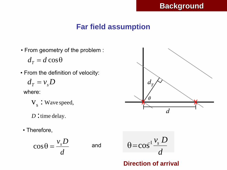
Far field assumption

• From geometry of the problem :

θ= cosddT

• From the definition of velocity:

Dvd sT =

. D delay time

speed, Wave

::vs

where:

• Therefore,

dDvs=θcos

dDvs1cos−=θ

Direction of arrival

and


Near field assumption

Where

•

L is the maximum length of the array

•

λ

is the wavelength of the acoustic field

R

L

λ<

22LR


Combined Approach

R

dL

λ<<

λ

22 22 LRdNear-Field Array/Far-Field sensor pair


Each angle is a function of delay, making position also a function of delay, which is unknown and need to be estimated.

Under near-field array/far-field sensor pair:

x

y

P

x*

y*

ba

dd

1θ2θ

21 θθ ≠

)tan()tan(

)]tan()[tan(2

12

12*

θ−θ

θ+θ−=

P

x

)tan()tan()tan()tan(

12

12*

θ−θθθ−

=Py

Therefore,

Combined Approach (Cont.)


Measurement model

)()()()()()(

212

111

tnDtstxtntstx

++α=+=

Where

• D is the delay,

• n1(t), n2(t) are all real, zero-mean,

jointly stationary independent random processes,

• s1(t) is assumed uncorrelated with n1(t) and n2(t).

Estimation AlgorithmsEstimation Algorithms

• A common method for finding D is to use the cross correlation function:

•

The argument that maximizes this function provides the estimate

of delay D:

)]()([)( 2121ττ −= txtxER xx

21xxRmax)arg(ˆ τ=D

Time-delay estimation


•

In Generalized Cross Correlation, pre-filters are used to improve the accuracy of the time delay results.

Cross Correlation D̂

)(1 fH

)(2 fH

Peak Detection

1x

2x

1y

2y

•

Each method of GCC is defined by its unique weighting function in the frequency domain, which acts as the filter before Cross Correlation takes place. Several well known methods exist for this process.

•

Roth Processor•

Smoothed Coherence Transform (SCOT)•

Phase Transform (PHAT)


•

Eckert Filter•

HT Processor•

Maximum Likelihood (ML)


DOA estimation based on time-delay estimates

•

At each pair of microphones

•

is estimated based on discrete samples, thus,

•

where , and

is the sample cross-correlation.

•

Therefore,

dDv is

i

ˆcos 1−=θ

s

isi fd

nv ˆcosˆ 1−=θ

si fnD /ˆˆ =iD̂

21

~max)arg(ˆ xxRn τ=

21

~xxR


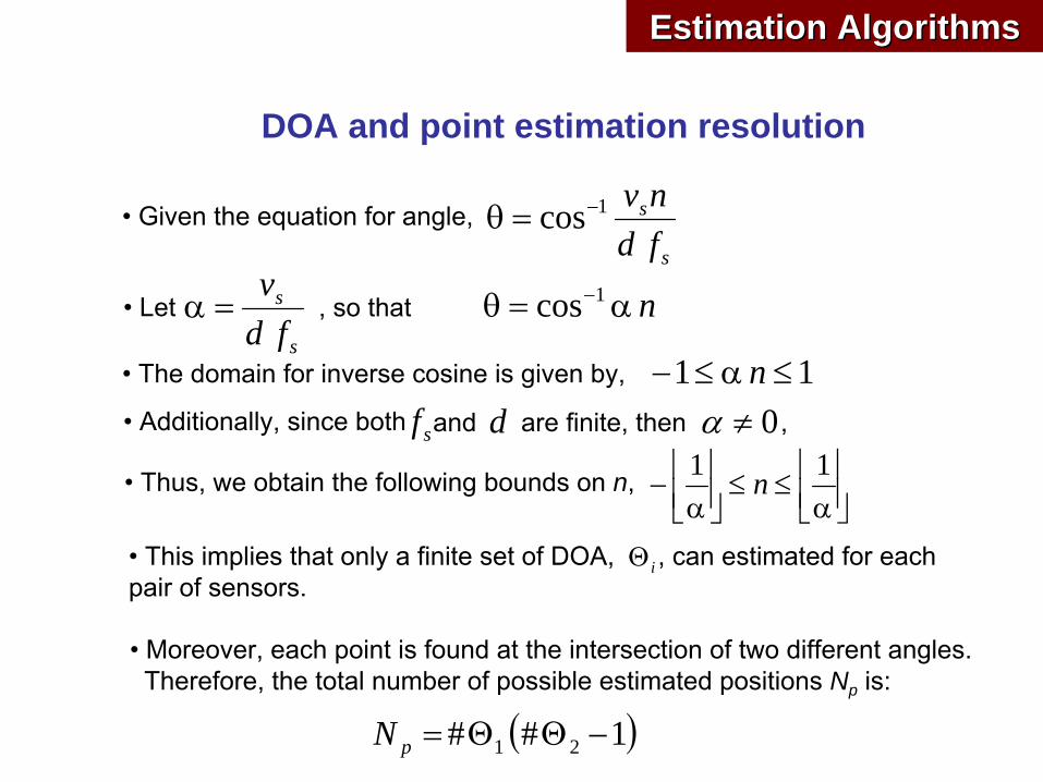
DOA and point estimation resolution

• Given the equation for angle,s

s

fdnv1cos−=θ

• Lets

s

fdv

=α , so that nα=θ −1cos

• The domain for inverse cosine is given by, 11 ≤α≤− n0≠α• Additionally, since both sf and d are finite, then ,

• Thus, we obtain the following bounds on n, ⎥⎦⎥

⎢⎣⎢α

≤≤⎥⎦⎥

⎢⎣⎢α

−11 n

•

This implies that only a finite set of DOA, , can estimated for each pair of sensors.

• Moreover, each point is found at the intersection of two different angles.Therefore, the total number of possible estimated positions Np is:

( )1## 21 −ΘΘ=pN

iΘ


•

If we use the minimum values proposed from the Nyquist

criterion, we are able to estimate only three points per pair.

ffs 2=Nyquist

Criteria: , 2λ

=d

Recall:s

s

fdv

=α

fvs=λwhere, 1

22

==f

fv

vs

sα

• With alpha equal to 1, we can only estimate DOA at 90, 0, and 180.

• The resolution is dependent on both spatial and temporal quantities.

DOA and point estimation resolution (Cont.)


• Using the following parameters:

2510385.0

/34020.

100,44

=⎥⎦⎥

⎢⎣⎢

====

α

αsmv

mdf

s

s

This leads to the possible number of angles per pair of sensors to be 51, making the total number of possible points 2550.

•

As the distance from the array increases, so the gap between the points also increases creating large regions of ambiguity.


Spatial Quantization

Higher Resolution

Large Region of Ambiguity


Spatial Quantization

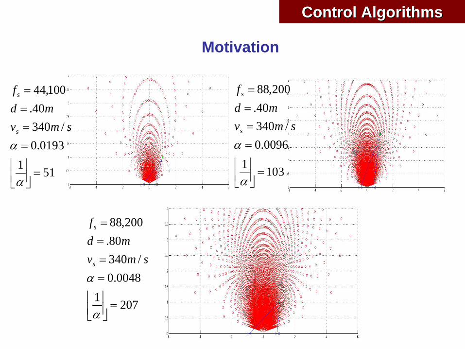
5110193.0

/34040.

100,44

=⎥⎦⎥

⎢⎣⎢

====

α

αsmv

mdf

s

s

10310096.0

/34040.

200,88

=⎥⎦⎥

⎢⎣⎢

====

α

αsmv

mdf

s

s

20710048.0

/34080.

200,88

=⎥⎦⎥

⎢⎣⎢

====

α

αsmv

mdf

s

s

Control AlgorithmsControl Algorithms

Motivation


Important Input Variables:

Previous Position

Critical Resolution

Estimated Source Position

Acoustic limitation Distance

Maximizing Resolution:

•

Question 1

–

Is the Microphone Array in near field or far field?

•

Question 2

–

Is the Microphone Array centered around the estimated source position?

•

Question 3

–

Are robots’

movement constrained by physical or acoustic limitations?

•

Question 4

–

I s the current resolution better than the previous resolution at the estimated position?

Heuristic Control Approach

-5 -4 -3 -2 -1 0 1 2 3 4 50

0.5

1

1.5

2

2.5

3

3.5

4

4.5

5

-5 -4 -3 -2 -1 0 1 2 3 4 50

0.5

1

1.5

2

2.5

3

3.5

4

4.5

5

-5 -4 -3 -2 -1 0 1 2 3 4 50

0.5

1

1.5

2

2.5

3

3.5

4

4.5

5

Xs = 1.949 Ys

= 2.045 Error = 0.0680

Xs = 2.323 Ys

= 2.405 Error = 0.5180

Xs = 1.949 Ys

= 1.944 Error = 0.0757


Heuristic Control Approach

Numerical example

NTXPair of Motors Source Position Estimation

Sensing Acoustic FieldPair of Microphones + DAQ

Sensing parameter adaptation

Robotic Platform 1 Computer for Central Processing

Feedback

NTXPair of Motors

Sensing Acoustic FieldPair of Microphones + DAQ

Robotic Platform 2


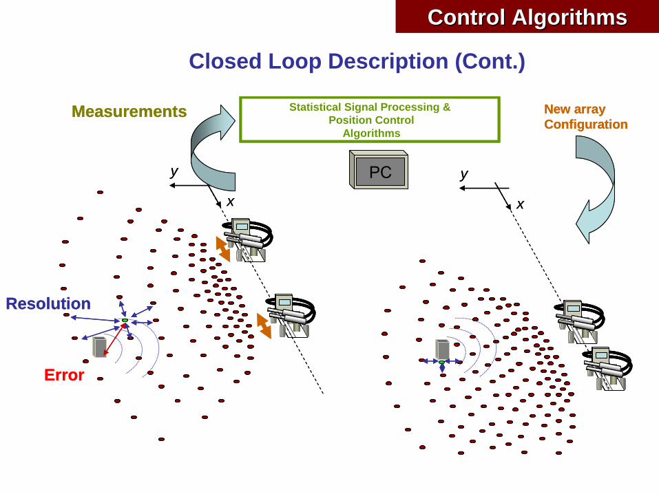
Closed Loop Description

Resolution

y

x

y

x

Error

PC

Statistical Signal Processing &Position Control

Algorithms

Measurements New array Configuration

Resolution

y

x

y

x

Error

PC

Statistical Signal Processing &Position Control

Algorithms

Measurements New array Configuration


Closed Loop Description (Cont.)

Hardware Design Software/InterfaceDesign Algorithm Design

Physical/Chemical/BiologicalBackground

Transducer/Sensor Selection

Data Acquisition System(sampling rate and resolution)

Signal Conditioning(analog filter, signal amplifier)

Graphical User Interface (GUI)Design

Real-time Data ProcessingArquitectures

Statistical Signal ProcessingAlgorithms

Preprocessing Algorithms(Digital filters: FIR, IIR)

Graphical display of variablesof interest

User-defined System and Algorithms

parameters

Microcontroller

Actuators (motors)

Robotic Platform Central Processing

Com

mun

icat

ion

Experimental SetupExperimental Setup

Hardware Design

R

L

x

y

x*

y*

?2 ?1

)tan()tan(

)]tan()[tan(2

12

12*

θ−θ

θ+θ−=

P

x


12

12*

θ−θθθ−= Py

P dd Sensor

Source

dvs )(cos Delay Time1−=θ

R

L

x

y

x*

y*

?2 ?1

R

L

x

y

x*

y*

R

L

RRRR

L

x

y

x*

y*

x

y

x*

y*

x

y

x*

y*

x

y

x*

y*

x

y

x*

y*

?2 ?1

)tan()tan(

)]tan()[tan(2

12

12*

θ−θ

θ+θ−=

P

x


12

12*

θ−θθθ−= Py

P dd Sensor

Source


Physical/Chemical/BiologicalBackground


Algorithm Design


)(1 fH

)(2 fH

Peak Detection

1x

2x

1y

2y


)(1 fH

)(2 fH

Peak Detection

1x

2x

1y

2y

R

L

x

y

x*

y*

?2 ?1

)tan()tan(

)]tan()[tan(2

12

12*

θ−θ

θ+θ−=

P

x


12

12*

θ−θθθ−= Py

P dd Sensor

Source


R

L

x

y

x*

y*

?2 ?1

R

L

x

y

x*

y*

R

L

RRRR

L

x

y

x*

y*

x

y

x*

y*

x

y

x*

y*

x

y

x*

y*

x

y

x*

y*

?2 ?1

)tan()tan(

)]tan()[tan(2

12

12*

θ−θ

θ+θ−=

P

x


12

12*

θ−θθθ−= Py

P dd Sensor

Source


Physical/Chemical/Biological Background Statistical Signal Processing Algorithms

)()()()()()(

212

111

tnDtstxtntstx

++α=+=

Measurement Model


Preprocessing Algorithms

• FIR filters

• IIR filters

dDv is

i

ˆcos 1−=θ

DOA estimation at each microphone


Algorithm Design (Cont.)

Statistical Signal Processing Algorithms

Higher Resolution

Region of Ambiguity

Higher Resolution

Region of Ambiguity

Microphones pairs

-5 -4 -3 -2 -1 0 1 2 3 4 50

0.5

1

1.5

2

2.5

3

3.5

4

4.5

5

-5 -4 -3 -2 -1 0 1 2 3 4 50

0.5

1

1.5

2

2.5

3

3.5

4

4.5

5

-5 -4 -3 -2 -1 0 1 2 3 4 50

0.5

1

1.5

2

2.5

3

3.5

4

4.5

5

Xs = 1.949 Ys = 2.045 Error = 0.0680Xs = 2.323 Ys = 2.405 Error = 0.5180 Xs = 1.949 Ys = 1.944 Error = 0.0757


Hardware Design

dbx RTA microphone Example of a DC Blocking Filter Diagram DAQ

Transducer/Sensor Selection Signal Conditioning Data Acquisition System

Microcontroller Actuators

NXT ARM7 Servomotor

Robotic Microphone array


Sensors

• Measurement microphone

Experimental SetupExperimental SetupHardware Design

dbx RTA microphone

• Polar Pattern : Omni-directional

• Element : Back Electret

Condenser

• Frequency : 20 Hz -

20 kHz

• Impedance : 250 30% (at 1,000Hz)

•

Sensitivity : -63 dB 3 dB ( 0 dB=1V/ microbar 1,000 Hz indicated by open circuit )

• Operating Voltage : Phantom power 15V D.C.

•

Condenser microphone:

the diaphragm acts as one plate of a capacitor, and the vibrations produce changes in the distance between the plates.

The capacitor requires to be polarized.

•

Electret

microphone: is a type of condenser microphone, which eliminates the need for a polarizing power supply by using a permanently-charged material.

•

Back electret:

An electret

film is applied to the back plate of the microphone capsule and

the diaphragm is made of an uncharged material

D.A.Q

•

The data acquisition system (DAQ) that is used for the acoustic sensing device is the National Instruments NI USB-6210:

16 analog inputs (16-bit, 400 kS/s)2 analog outputs (16-bit, 250 kS/s) 32 digital I/O 2 32-bit counters

• The maximum sampling rate is 400 kS/s

aggregate.

Experimental SetupExperimental SetupHardware Design

Software/Interface Design

Graphical display of variablesof interest

Graphical User Interface (GUI) Design

User-defined System and Algorithms

parametersReal-time Data Processing

Architectures

GUI using Matlab

Real time source location

Spectrogram

Estimated location

• Sensor array configuration

• Data acquisition system

• Preprocessing filters

• Cross-correlation algorithm


Real-time Data Processing Architectures

Experimental SetupExperimental SetupSoftware/Interface Design

•

The proposed system requires the synchronization of signal waveform generation, sound output functionality, data acquisition, signal

processing, plotting of the source estimation, and constructive commands for

robot movement, all occurring in parallel with one another.

•

This system can be modeled as a constant flow of data, which, when considered to be a sequence of events, occurs as is shown

Source location

algorithm

Source location

algorithm

Waveform generatorWaveform generator

Sound output & speaker


Data Acquisition

Data Acquisition

FilterFilter

Cross correlation

Cross correlationIncoming

angle algorithm

Incoming angle

algorithm

Robot controller

Robot controller

Array of microphones


Source location

algorithm

Source location

algorithm

Waveform generatorWaveform generator



Data Acquisition

Data Acquisition

FilterFilter

Cross correlation

Cross correlationIncoming

angle algorithm

Incoming angle

algorithm

Robot controller

Robot controller





•

In real time the processes occurring in parallel with respect to one another and can be more accurately represented by the figure in the left.

•

To implement parallel processes we use a Data Flow Programming approach in which the flow of data rather than the sequential order of commands determines the execution order of block diagram elements.

•

A block diagram node executes when it receives all required inputs. When a node executes, it produces output data and passes the data to the next node in the dataflow path. The movement of data through the nodes determines the execution order and functions on the block diagram.

Sound Output & Waveform Generation


Data Acquisition

& Mics

Data Acquisition

& Mics

Processing & PlottingProcessing & Plotting

Controller & RobotsController & Robots



Data Acquisition

& Mics

Data Acquisition

& Mics



Given the parallel architecture that real-time processing demands, we opted to build our system in the dataflow programming environment, LabVIEW.





Data Acquisition

& Mics

Data Acquisition

& Mics





Data Acquisition

& Mics

Data Acquisition

& Mics



•

To provide the system with a centralized control, we used LabVIEW’s

front panel interface.

•

The G.U.I provides the user with an interactive tool that manages all of the acquisition, processing, and robot movement and analysis.

•

This approach allows the user to vary parameters rapidly in a user friendly environment.

•

This approach also allowed us to expand our analytical tools and explore simulated concepts while comparing them to actual experimental results

Centralized Control and Signal Processing


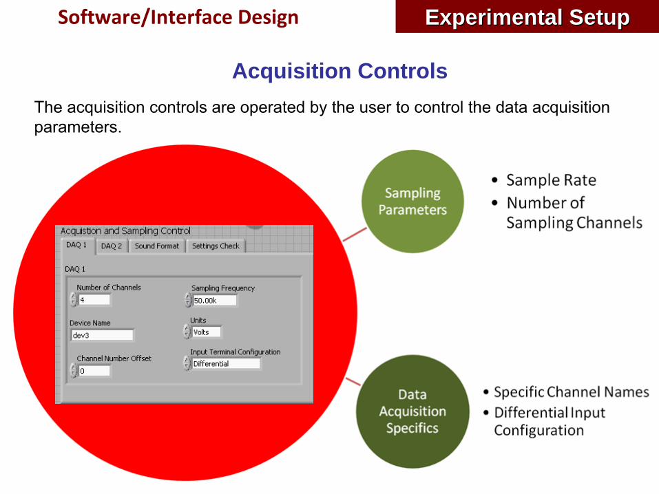
Acquisition ControlsThe acquisition controls are operated by the user to control the

data acquisition parameters.

Software/Interface Design Experimental SetupExperimental Setup

Signal Generation Controls

Signal Generation controls are operated by the user to control the type of the outgoing waveform.


Processing and Filtering

The Processing controls provide the user with the ability to filter the data using a particular cutoff frequency. The GCC method is also selected on this menu.


Robotic Movement Controls

Initial robot position and rotation is chosen. Limitations on movement based on physical surroundings are entered. Parameters algorithm uses to

determine real time movement are also used.


Simulation Controls

Simulation controls set the simulated position of the sound source. They also control simulated noise and sampling frequency.


Analysis IndicatorsThese indicators provides the analytical tools for the user to view the data and estimations. The estimations from processing are shown for the delays, angles, and position. Plots are also displayed in real time.


Available Plot Types

The plot types available in the GUI are shown below.


Demonstration at the WUSTL Undergraduate Research Symposium,Demonstration at the WUSTL Undergraduate Research Symposium,October 24October 24thth, 2009, 2009

DemonstrationDemonstration

Demonstration at BH 316 November 2009Demonstration at BH 316 November 2009

DemonstrationDemonstration

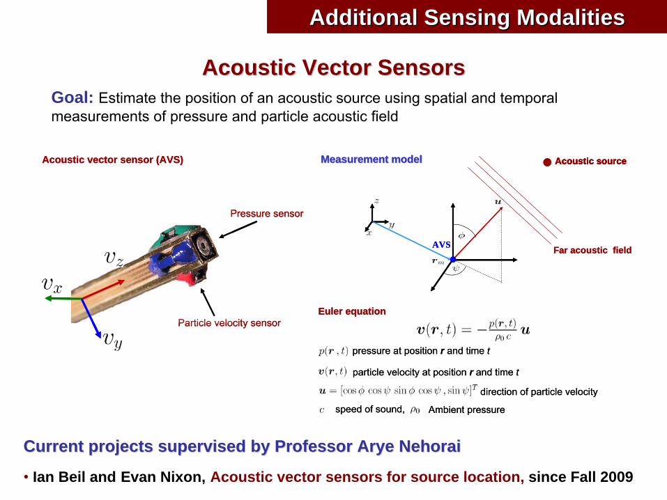
Acoustic Vector SensorsAcoustic Vector Sensors

Current projects supervised by Professor Current projects supervised by Professor AryeArye NehoraiNehorai

• Ian Beil and Evan Nixon, Acoustic vector sensors for source location, since Fall 2009

Microphones

Goal: Estimate the position of an acoustic source using spatial and temporal measurements of pressure and particle acoustic field

Pressure sensor

Particle velocity sensor

Acoustic vector sensor (AVS)

Pressure sensor

Particle velocity sensor

Acoustic vector sensor (AVS) Measurement modelMeasurement model Acoustic source

AVS Far acoustic field

Acoustic sourceMeasurement modelMeasurement model Acoustic source

AVS Far acoustic field

Acoustic source

Euler equation

pressure at position r and time t

particle velocity at position r and time t

direction of particle velocity

speed of sound, Ambient pressure

Euler equation

pressure at position r and time t

particle velocity at position r and time t

direction of particle velocity

speed of sound, Ambient pressure

Additional Sensing ModalitiesAdditional Sensing Modalities

Signal conditioner

DAQ

Array of AVS Capon Spectra

Signal conditioner

DAQ

Array of AVS Capon Spectra

Above: Diagram of experimental setup; Power distribution as a function of azimuth and elevation. The red arrow indicates the maximum spectral value.

Right: Experimental setup at SPIRIT LAB

Additional Sensing ModalitiesAdditional Sensing Modalities

Acoustic Vector Sensors (Cont.)Acoustic Vector Sensors (Cont.)

SummarySummary

•

We proposed a novel concept and built a robotic platform that allows to improve the performance in estimating adaptively the location of

an acoustic source in 2D using an array of microphones

•

We proposed a general methodology for implementing robotic sensing systems which facilitates the construction of our experimental setup.

•

We implemented real-time processes using a data flow programming approach which allows to track a moving acoustic source in 2D

Future WorkFuture Work•

We are working on adding additional degrees of freedom to the robots such as rotation and displacement in 2D.

•

We will implement a wireless communication between the robots and the central processing unit.

ConclusionConclusion

robotic microphone arrays - washington university in st. louis

Documents