RoboSimReference ManualAna CavalcantiPedro Ribeiro

Alvaro Miyazawa

Augusto SampaioMadiel Conserva Filho

André Didier

April 16, 2019

Abstract

In this report, we describe a UML-like notation called RoboSim, designedspecifically for simulation of autonomous and mobile robots, and includingtimed primitives. We provide a reference manual for RoboSim. We describethe syntax, the well-formedness conditions and semantics of RoboSim. Wealso present three case studies and show how we can use RoboSim modelsto check if a simulation is consistent with a functional design written in aUML-like notation.1

1The interested reader can reproduce the verification of all examples presented in this Reference Manual.Further information is available at https://www.cs.york.ac.uk/circus/RoboCalc/case_studies.

Contents

1 Introduction 7

2 RoboChart and the need for RoboSim 9

3 RoboSim metamodel 17

4 Well-formedness Conditions 214.1 Robotic Platforms . . . . . . . . . . . . . . . . . . . . . . . . . . . . . . . 214.2 Modules . . . . . . . . . . . . . . . . . . . . . . . . . . . . . . . . . . . . . 214.3 Controllers . . . . . . . . . . . . . . . . . . . . . . . . . . . . . . . . . . . 224.4 State Machine . . . . . . . . . . . . . . . . . . . . . . . . . . . . . . . . . . 224.5 Transitions . . . . . . . . . . . . . . . . . . . . . . . . . . . . . . . . . . . 234.6 Statements . . . . . . . . . . . . . . . . . . . . . . . . . . . . . . . . . . . 234.7 Events . . . . . . . . . . . . . . . . . . . . . . . . . . . . . . . . . . . . . . 24

5 RoboSim Semantics 255.1 CSP and tock-CSP . . . . . . . . . . . . . . . . . . . . . . . . . . . . . . . 255.2 Overview . . . . . . . . . . . . . . . . . . . . . . . . . . . . . . . . . . . . 285.3 Formalisation . . . . . . . . . . . . . . . . . . . . . . . . . . . . . . . . . . 39

5.3.1 Memory . . . . . . . . . . . . . . . . . . . . . . . . . . . . . . . . . 535.3.2 Clocks . . . . . . . . . . . . . . . . . . . . . . . . . . . . . . . . . . 535.3.3 Expressions . . . . . . . . . . . . . . . . . . . . . . . . . . . . . . . 585.3.4 Auxiliary Functions . . . . . . . . . . . . . . . . . . . . . . . . . . 655.3.5 Waiting Condition as CSP processes . . . . . . . . . . . . . . . . . 69

5.4 Automated verification . . . . . . . . . . . . . . . . . . . . . . . . . . . . . 765.4.1 Relating design and simulation models . . . . . . . . . . . . . . . . 775.4.2 Verification . . . . . . . . . . . . . . . . . . . . . . . . . . . . . . . 81

6 Examples 876.1 Square . . . . . . . . . . . . . . . . . . . . . . . . . . . . . . . . . . . . . . 87

2

6.1.1 RoboChart model . . . . . . . . . . . . . . . . . . . . . . . . . . . . 876.1.2 RoboSim model . . . . . . . . . . . . . . . . . . . . . . . . . . . . . 88

6.2 Transporter . . . . . . . . . . . . . . . . . . . . . . . . . . . . . . . . . . . 916.2.1 RoboChart model . . . . . . . . . . . . . . . . . . . . . . . . . . . . 916.2.2 RoboSim model . . . . . . . . . . . . . . . . . . . . . . . . . . . . . 94

6.3 Alpha Algorithm . . . . . . . . . . . . . . . . . . . . . . . . . . . . . . . . 966.3.1 RoboChart model . . . . . . . . . . . . . . . . . . . . . . . . . . . . 966.3.2 RoboSim model . . . . . . . . . . . . . . . . . . . . . . . . . . . . . 97

7 Conclusions 100

A Complete Metamodel 101

Index of Semantic Rules 106

Index of Calls to Semantic Rules 108

List of Figures

2.1 RoboChart: obstacle detection . . . . . . . . . . . . . . . . . . . . . . . . . 102.2 Cycle of a simulation . . . . . . . . . . . . . . . . . . . . . . . . . . . . . . 122.3 RoboSim: obstacle detection . . . . . . . . . . . . . . . . . . . . . . . . . . 142.4 RoboSim obstacle detection - alternative . . . . . . . . . . . . . . . . . . . 16

3.1 RoboSim metamodel . . . . . . . . . . . . . . . . . . . . . . . . . . . . . . 18

5.1 Structure of RoboSim tock-CSP semantics . . . . . . . . . . . . . . . . . . 285.2 Semantics of a RoboSim state machine . . . . . . . . . . . . . . . . . . . . 335.3 Semantics of a RoboSim module . . . . . . . . . . . . . . . . . . . . . . . . 395.4 Simulation machine: missing entry action for state SMoving . . . . . . . . 845.5 Simulation machine: missing guard to state STurning . . . . . . . . . . . . 845.6 Simulation machine: swapping guards in transitions from DMoving . . . . 855.7 Simulation machine: possibly ignoring an obstacle occurrence . . . . . . . 855.8 Simulation machine: wrong cycle allocation . . . . . . . . . . . . . . . . . 86

3

6.1 RoboChart: square trajectory state machine. The module contains a singlecontroller, which contains this machine. . . . . . . . . . . . . . . . . . . . 88

6.2 RoboSim: square trajectory state machine . . . . . . . . . . . . . . . . . . 896.3 RoboChart state machine of the Transporter . . . . . . . . . . . . . . . . . 926.4 RoboSim model of the Transporter . . . . . . . . . . . . . . . . . . . . . . 956.5 RoboChart: Alpha Algorithm . . . . . . . . . . . . . . . . . . . . . . . . . 976.6 Simulation machine of the Alpha Algorithm in RoboSim . . . . . . . . . . 98

List of rules

1 Semantics of modules . . . . . . . . . . . . . . . . . . . . . . . . . . . . . 402 Module or controller memory . . . . . . . . . . . . . . . . . . . . . . . . . 423 Composition of controllers . . . . . . . . . . . . . . . . . . . . . . . . . . 424 Semantics of controllers . . . . . . . . . . . . . . . . . . . . . . . . . . . . 435 Cycle for modules and controllers . . . . . . . . . . . . . . . . . . . . . . 446 Composition of machines . . . . . . . . . . . . . . . . . . . . . . . . . . . 447 State machine . . . . . . . . . . . . . . . . . . . . . . . . . . . . . . . . . 458 Cycle for machines . . . . . . . . . . . . . . . . . . . . . . . . . . . . . . . 469 Clocks for machines . . . . . . . . . . . . . . . . . . . . . . . . . . . . . . 4710 Buffer for machines . . . . . . . . . . . . . . . . . . . . . . . . . . . . . . 4811 Behaviour of state machine . . . . . . . . . . . . . . . . . . . . . . . . . . 4912 State-machine memory . . . . . . . . . . . . . . . . . . . . . . . . . . . . 5013 memoryTransition function . . . . . . . . . . . . . . . . . . . . . . . . . . 5114 ExecTrigger . . . . . . . . . . . . . . . . . . . . . . . . . . . . . . . . . . 5115 Semantics of final states . . . . . . . . . . . . . . . . . . . . . . . . . . . . 5216 Get and Set channels . . . . . . . . . . . . . . . . . . . . . . . . . . . . . 5217 Trigger events . . . . . . . . . . . . . . . . . . . . . . . . . . . . . . . . . 5218 Operation call . . . . . . . . . . . . . . . . . . . . . . . . . . . . . . . . . 5319 Semantics of triggers for memory . . . . . . . . . . . . . . . . . . . . . . . 5320 clockVariables function . . . . . . . . . . . . . . . . . . . . . . . . . . . . 5321 clockResets function . . . . . . . . . . . . . . . . . . . . . . . . . . . . . . 5422 stmClocks function . . . . . . . . . . . . . . . . . . . . . . . . . . . . . . 54

4

23 alphaClockReset function . . . . . . . . . . . . . . . . . . . . . . . . . . . 5424 alphaClockReset function . . . . . . . . . . . . . . . . . . . . . . . . . . . 5425 alphaClockReset function . . . . . . . . . . . . . . . . . . . . . . . . . . . 5526 alphaClockReset function . . . . . . . . . . . . . . . . . . . . . . . . . . . 5527 alphaClockResetCallArgs function . . . . . . . . . . . . . . . . . . . . . . 5528 alphaClockReset function . . . . . . . . . . . . . . . . . . . . . . . . . . . 5529 alphaClockReset function . . . . . . . . . . . . . . . . . . . . . . . . . . . 5630 alphaClockReset function . . . . . . . . . . . . . . . . . . . . . . . . . . . 5631 alphaClockReset function . . . . . . . . . . . . . . . . . . . . . . . . . . . 5632 alphaClockReset function . . . . . . . . . . . . . . . . . . . . . . . . . . . 5633 alphaClockReset function . . . . . . . . . . . . . . . . . . . . . . . . . . . 5734 alphaClockReset function . . . . . . . . . . . . . . . . . . . . . . . . . . . 5735 alphaClockReset function . . . . . . . . . . . . . . . . . . . . . . . . . . . 5736 alphaClockReset function . . . . . . . . . . . . . . . . . . . . . . . . . . . 5737 alphaClockReset function . . . . . . . . . . . . . . . . . . . . . . . . . . . 5838 Semantics of expressions . . . . . . . . . . . . . . . . . . . . . . . . . . . 5839 Semantics of and expression . . . . . . . . . . . . . . . . . . . . . . . . . 5840 Semantics of array expression . . . . . . . . . . . . . . . . . . . . . . . . . 5841 Semantics of boolean expression . . . . . . . . . . . . . . . . . . . . . . . 5942 Semantics of call expression . . . . . . . . . . . . . . . . . . . . . . . . . . 5943 Semantics of concatenation expression . . . . . . . . . . . . . . . . . . . . 5944 Semantics of not equal expression . . . . . . . . . . . . . . . . . . . . . . 6045 Semantics of division . . . . . . . . . . . . . . . . . . . . . . . . . . . . . 6046 Semantics of equality . . . . . . . . . . . . . . . . . . . . . . . . . . . . . 6047 Semantics of greater or equal expression . . . . . . . . . . . . . . . . . . . 6048 Semantics of greater than . . . . . . . . . . . . . . . . . . . . . . . . . . . 6149 Semantics of if and only if expression . . . . . . . . . . . . . . . . . . . . 6150 Semantics of implication . . . . . . . . . . . . . . . . . . . . . . . . . . . 6151 Semantics of integer expression . . . . . . . . . . . . . . . . . . . . . . . . 6152 Semantics of less or equal expression . . . . . . . . . . . . . . . . . . . . . 6253 Semantics of less than . . . . . . . . . . . . . . . . . . . . . . . . . . . . . 6254 Semantics of minus . . . . . . . . . . . . . . . . . . . . . . . . . . . . . . 6255 Semantics of modulus . . . . . . . . . . . . . . . . . . . . . . . . . . . . . 6256 Semantics of multiplication . . . . . . . . . . . . . . . . . . . . . . . . . . 6357 Semantics of arithmetic negation . . . . . . . . . . . . . . . . . . . . . . . 6358 Semantics of logical negation . . . . . . . . . . . . . . . . . . . . . . . . . 63

5

59 Semantics of or expression . . . . . . . . . . . . . . . . . . . . . . . . . . 6360 Semantics of parenthesised expression . . . . . . . . . . . . . . . . . . . . 6461 Semantics of plus . . . . . . . . . . . . . . . . . . . . . . . . . . . . . . . 6462 Semantics of range expression . . . . . . . . . . . . . . . . . . . . . . . . 6463 Semantics of sequence expression . . . . . . . . . . . . . . . . . . . . . . . 6464 Semantics of set expression . . . . . . . . . . . . . . . . . . . . . . . . . . 6565 Semantics of tuple expression . . . . . . . . . . . . . . . . . . . . . . . . . 6566 Function allVariables . . . . . . . . . . . . . . . . . . . . . . . . . . . . . 6567 Function allLocalVariables . . . . . . . . . . . . . . . . . . . . . . . . . . 6568 Function allConstants . . . . . . . . . . . . . . . . . . . . . . . . . . . . . 6669 Function requiredVariables . . . . . . . . . . . . . . . . . . . . . . . . . . 6670 Function allTransitions . . . . . . . . . . . . . . . . . . . . . . . . . . . . 6671 triggerEvent function . . . . . . . . . . . . . . . . . . . . . . . . . . . . . 6672 Composition of states . . . . . . . . . . . . . . . . . . . . . . . . . . . . . 6773 Restricted semantics of states . . . . . . . . . . . . . . . . . . . . . . . . . 6774 Flow events . . . . . . . . . . . . . . . . . . . . . . . . . . . . . . . . . . . 6875 Function transitionsFrom . . . . . . . . . . . . . . . . . . . . . . . . . . . 6876 Function states . . . . . . . . . . . . . . . . . . . . . . . . . . . . . . . . . 6877 Constants Initialisation for Controllers and Modules . . . . . . . . . . . . 6878 compileWC function . . . . . . . . . . . . . . . . . . . . . . . . . . . . . . 7078 compileWC function . . . . . . . . . . . . . . . . . . . . . . . . . . . . . . 7178 compileWC function . . . . . . . . . . . . . . . . . . . . . . . . . . . . . . 7278 compileWC function . . . . . . . . . . . . . . . . . . . . . . . . . . . . . . 7378 compileWC function . . . . . . . . . . . . . . . . . . . . . . . . . . . . . . 7478 compileWC function . . . . . . . . . . . . . . . . . . . . . . . . . . . . . . 75

6

Chapter 1

Introduction

In this report, we present a state-machine based notation, called RoboSim, designedspecifically for the modelling of verified simulations for robotic applications. As a graph-ical notation, RoboSim is intended to be more appealing than programming notations;furthermore, a model in RoboSim should be considered as an intermediate, implementa-tion independent, representation that can be translated into languages used by severalwell-established simulators such as Netlogo [23], MASON [11], JASON [1], Argos [17],Enky (home.gna.org/enki/), Microsoft Robotics Developer Studio (www.microsoft.com/robotics), Webots, and Simulink + Stateflow [12, 13]. The graphical notationof RoboSim is inspired on RoboChart [21], a UML-like notation designed for robotics.However, as a simulation notation, it has the following

CFootBot = EntryMoving ; Obstacle; EntryTurning ;

• A model in RoboSim specifies a cyclic mechanism, as is usual in languages likeNetlogo and Stateflow, among others.

• The cycle itself is a separate mechanism from the executing machine; a RoboSimmodel is formed of the parallel execution of the cycle and the machine.

• Time information is restricted to the cycle; the model of the machine is untimed.

• The visible events are readings and writings in registers of sensors and actuators.

• These events are always available.

Additionally, RoboSim has some distinguishing features.

• The cycle step can be more flexibly defined than, for instance, in Stateflow. Par-ticularly, a step is not constrained to entering a single state of the machine.

7

• A formal semantics for RoboSim is given in the same framework as that for RoboChart,which allows the definition of a notion of correct simulation with respect to the moreabstract RoboChart model.

• Other relevant properties of a simulation can also be mechanically checked like.For instance, the improper execution of the same operation more than once in asame cycle.

Like RoboChart, apart from the state-machine itself, RoboSim includes elements to or-ganise specifications, fostering reuse and taming complexity.

The state-machine notation is fully specified, including an action language and constructsto specify timing and properties. Operations used in a state machine can be taken froma domain-specific API or defined by other state machines; communication between statemachines is synchronous. Operations can be given pre and postconditions.

In this report, we formalise the semantics of RoboSim using CSP [19]. Importantly, CSPis a front end for a mathematical model that supports a number of analysis techniquesthat allow, for example, checking the validity of a simulation. For that we can usemodel-checking, which provides a high degree of automation, as well as more powerful(but not automatic) verification based on theorem proving. Use of CSP enables modelchecking with FDR [8]. On the other hand, CSP has an underlying model based Hoareand He’s Unifying Theories of Programming [10] that makes our core semantics adequatefor theorem proving and for extension to deal, for instance, with probability [25].

The remainder of this manual is structured as follows. In Chapter 2 we briefly presentRoboChart the language we use to describe designs of robotic applications, and to showhow we can relate RoboSim and design models. Using RoboChart we also give in Chap-ter 2 examples that illustrate the need for separate design and simulation notations.Chapter 3 presents the RoboSim metamodel, and Chapter 4 defines the well-formednessconditions. The semantics is presented in Chapter 5. Chapter 6 presents some casestudies. Finally, Chapter 7 concludes with a summary of the results and future work.

8

Chapter 2

RoboChart and the need for RoboSim

We have previously presented RoboChart [18], a state-machine based notation that canbe defined as a UML profile. RoboChart is distinctive in three aspects. First, it providesarchitectural constructs to identify the requirements for a robotic platform, and a (par-allel) design of controllers. Second, it supports definition of time budgets for operations,and deadlines based on events and states. Finally, it has a CSP semantics that can beautomatically calculated.

We use the toy model in Figure 2.1 to illustrate RoboChart, and later RoboSim. A roboticsystem is defined in RoboChart by a module. In our example, it is called CFootBot, andspecifies a robot that can move around, detect obstacles, and stop. A module contains aplatform and one or more controllers that run on this platform.

The robotic platform FootBot defines the interface of the system with its environment, viavariables, operations, and events. In our example, the operation move(lv,av) can be usedto set the robot into motion with linear speed lv and angular speed av. The operationstop can be used to instruct the robot to stop (before changing direction, for example).The event obstacle occurs when the robot gets close to any object in its environment;it is an abstraction of a sensor that detects obstacles. The variables, operations, andevents of a platform characterise also the facilities that an actual platform must provideto support the implementation of the system.

There may be one or more controllers, interacting with the platform via asynchronousevents, and between them via synchronous or asynchronous events. In our simple exam-ple, we have just a single controller Movement. The behaviour of a controller is definedby one or more state machines, specifying threads of execution. Again, in our simpleexample, the behaviour of Movement is defined just by the machine SMovement.

Interfaces can group variables, operations, and events. In Figure 2.1, the interface Move-mentI has only the operations move(lv,av) and stop(), provided by the robotic platform,

9

Robotic Platform Controller State machineDefined Interface Provided interface Required interfaceVariable declaration Constant OperationEvent Event Initial junction

Figure 2.1: RoboChart: obstacle detection

and required by the controller and state machines. ObstacleI has just the event obstacle,which is used in the platform, the controller, and the state machine. Libraries containingdefinitions of platforms and operations may be provided for reuse in the modelling ofrobotic systems.

Connections in the module define the data flow among the platform and the controllers.In general, different events may be connected, as long as they have the same type, or notype. Types are used when an event communicates an input or output value. Connectionsin a controller define the flow to, from, and among machines.

State machines are similar to those in UML, except that they have a well defined actionlanguage, and time primitives. In our example, upon entry in the state Moving, aftercalling the operation move(lv,0), the robot waits for one time unit. Operation calls,like move(lv,0), take no time; move(lv,0) can be, for example, implemented as a simpleassignment to the register of an actuator. The machine, however, is blocked by wait(1)for one time unit (which is a budget for the platform to react to this operation) beforeit completes entry to Moving.

10

In general, assignments and other data operations take no time. Equally, operationcalls, in principle, take no time. An operation, however, can itself be defined by a statemachine that uses the time primitives to define budgets. In addition, if an operation isleft completely undefined, that is, just a declaration is given, it can take an arbitraryamount of time. In our example, move is defined to terminate (assertion [terminates]),and since it is not given any other explicit definition using time primitives, it takes notime. Budgets need to be explicitly defined via the wait primitive.

SMovement declares a clock MBC. In Moving, when an obstacle is detected, MBC isreset (#MBC), the operation stop() is called, and then the machine may wait for one timeunit. After the wait, if any, the machine moves to the state Turning. A wait statementwait([0,1]) is nondeterministic: it can block for 0 or 1 time units. The nondeterminismhere may capture, for instance, that the robot may stop virtually instantaneously, ortake some (small) amount of time.

In the state Turning, a call move(0,av) turns the robot. A transition back to the stateMoving is guarded by since(MBC) >= PI/av. As soon as the guard is satisfied, thetransition is taken. The guard requires that the value of MBC is greater than or equalto that of PI/av, to ensure that the robot waits enough time to turn PI degrees, beforegoing back to Moving and proceeding in a straight line again. PI, lv, and av are constantsloosely defined.

Although not illustrated in Figure 2.1, we can define deadlines. For instance, the occur-rence of an event requires interaction with the environment, and so there is no guaranteeof how much time passes before an event occurs. For example, in Moving, an arbitraryamount of time may pass before an obstacle is detected. If appropriate, we can define adeadline, as an imposition on the environment as to the maximum amount of time thatmay pass.

A more complete description of RoboChart is available in [14, 18], and in the referencemanual [21]. Its core concepts (state machines, time budgets, and so on) are common tocyber-physical systems in general. It is the terminology and support provided with thelanguage (in the form of libraries of definitions of platforms and operations, examples,guidelines for use, and so on) that makes it distinctively for the design of robotic systems.RoboChart models are akin to those used in the robotics literature [5, 16, 2, 22]. Theyare, however, not simulation models, and, if used as a guide to develop a simulation, theyleave some important questions unanswered.

11

while true

registerRead

exec

registerWrite

cycleperiod

{wait(p)

Figure 2.2: Cycle of a simulation

First of all, irrespective of the simulator used, a simulation is a cyclic mechanism whosecontrol flow is as described in Figure 2.2. It normally proceeds indefinitely, with termi-nation determined only by a time limit. In each cycle, the simulation reads some inputs,which correspond to registers of the sensors, executes computations to process that inputand calculate outputs, and then writes those outputs to the registers of the actuators.A simulation takes an idealised view of time: input, computation, and output take placeinfinitely fast at the sample time, and then a period of quiescence follows. The amountof time of quiescence and the sample times are determined by the period.

In contrast, a RoboChart model, like those often written by roboticists to describe theirdesigns, is not cyclic. In our small example, the machine SMovement evolves in a cycle,from Moving to Turning and back, but that is not the cycle of the simulation. First ofall, there is no fixed period for that cycle, since, unless we know the exact configurationof the environment and starting point of the robot, we do not know when an obstacle isgoing to be detected. There may even be no obstacle at all. Second, the simulation cycledetermines when the register of the obstacle sensor is read, and so it needs to be muchfaster than the cycle in the RoboChart machine.

Therefore, when using a RoboChart model to guide the development of a simulation,there is no indication of the simulation cycle. More importantly, there is, therefore, noindication of the actions and transitions that are executed or considered for execution ineach cycle. In summary, there is no support for the complex task of scheduling.

12

Moreover, there are questions that cannot even be asked in a meaningful way. Forexample, in the context of a simulation, if an event occurs, it is recorded in a register,and it may be relevant to define when it should be cleared. For example, if an obstacle isdetected while SMovement is in the state Turning, that event is ignored. In a simulation,however, the question arises of whether the register should be cleared or not, so that theevent can be handled when SMovement is back in the state Moving. Depending on thetime the robot takes to turn and on the cycle of the simulation, different answers maybe appropriate. If the turning is fast, we may need to retain the event for immediateaction after turning. If it is slow, an obstacle seen during the turning may no longer bean issue when the robot finishes turning, and the right decision is to clear the registerthat records the event unless an obstacle is still sensed.

Finally, a simulation is typically a deterministic program. For that, it needs to prioritiseevents via specification of behaviour also in their absence. For example, in a statewith transitions triggered by two different events e1 and e2, if both events occur, eithertransition can take place, and the choice is nondeterministic. A simulation typicallyprioritises one of them. This is achieved by handling the event with lower priority onlywhen that of higher priority does not occur. So, it needs to specify behaviour in theabsence of an event. Yet, if the particular priority to be adopted is not important, theRoboChart design model does not enforce any particular prioritisation. Whereas it is notpossible to express this priority in a standard state-machine model, as we cannot specifybehaviour in the absence of an event, in a simulation the values of the registers, sayassociated with the events e1 and e2, allows such a control.

RoboSim addresses the issues above: support for scheduling, recording and clearing ofevent occurrences, and specification of behaviour in the absence of an event. This isachieved by defining a cyclic model, still potentially nondeterministic, where event oc-currences are captured by boolean variables, associated with additional variables whenthey communicate values. The definition of the cycle period and the scheduling for eachcycle are explicit.

As an example, we consider the simulation of our simple robot in Figure 2.3. Its overallstructure (module and controller) is similar to that of the RoboChart model in Figure 2.1,but, in general, a simulation may have an entirely different structure from that of acorresponding RoboChart model, for optimisation purposes, for instance.

13

In Figure 2.3, the module is SimCFootBot; it is composed by the FootBot platform and theSimMovement controller that has a reference to a single simulation machine SimSMove-ment. Essentially, the module differs from that in the RoboChart model just in thatit specifies the cycle period: it includes a (simple) predicate stating cycle == 1. Simi-larly, the controller SimMovement differs from Movement just in the inclusion of the cycledefinition.

Figure 2.3: RoboSim: obstacle detection

The machine SimSMovement has the same local constants PI, lv, and av, and clock MBCdefined in the RoboChart machine Movement. The event obstacle declared in the inter-face ObstacleI is an input, and the operations move and stop declared in the interfaceMovementI are outputs. Inputs and outputs are explicitly distinguished in RoboSim.

As already said, a RoboSim model specifies a cyclic mechanism; a special marker eventexec defines points where behaviour evolution must stop until the next cycle. In eachcycle, inputs are read from registers, processed, outputs are written to registers, andthen time elapses in a period of quiescence until the next cycle (see Figure 2.2). Duringprocessing, the simulation machine takes control of execution until progress requires the(next) occurrence of exec.

The visible behaviour is the reading and writing of registers, which is ultimately char-acterised by the inputs and outputs. Their values capture interactions correspondingto RoboChart platform events, access to platform variables, and calls to platform oper-ations. For instance, the event obstacle in Figure 2.1 is captured in our example as aregister with a boolean value indicating whether an obstacle has been detected or not.

14

The boolean variable $obstacle corresponding to this input is used in guards, not triggers,of transitions. So, the only trigger used in RoboSim is exec.

The overall behaviour of SimSMovement is as follows. The first cycle starts with thetransition from the initial junction to the SMoving state; its entry action records thatmove must be called, as indicated by $move(lv,0), with the $ as a reminder that theoperation is not called immediately. Afterwards, it changes to the DMoving state, whereit waits for the next cycle, because there are no transitions from DMoving not triggeredby exec (the only possible trigger in RoboSim). This corresponds to the action wait(1) inthe RoboChart design model, considering that the cycle period of the simulation is also1. If we had a different wait time in the design, we would need either to change the sizeof the cycle, or to change the RoboSim diagram to wait the right number of cycles.

In the next cycle, SimSMovement checks whether an obstacle has been perceived. If not,it remains in DMoving. Otherwise, it moves to STurning, when it resets the MBC clock,records that stop and then move must be called and moves to DTurning, all in one cycle.This defines a simulation that implements the nondeterministic wait([0,1]) by choosingwait(0), which has no effect: it is just a skip statement that terminates immediately.

In the subsequent cycle, it remains in DTurning if the amount of time since MBC hasbeen reset is less than PI/av, otherwise, it returns to SMoving. Here, the check of theclock can be delayed until the next cycle because PI is always greater than 0, so the statechange cannot happen in the same cycle.

An alternative RoboSim model that is also correct with respect to the RoboChart modelin Figure 2.1 is presented in Figure 2.4. In this case, the nondeterministic wait([0,1]) isimplemented by choosing wait(1). So, the transition with guard $obstacle leads to a stateWaiting, from which progress can be made only in the next cycle. Yet another option isa RoboSim model that preserves the nondeterminism. For example, we could have twotransitions with guard $obstacle (and the same action): one leading to Waiting, like inFigure 2.4, and another leading directly to STurning.

Finally, we observe that, without the wait(1) in the entry action of the state Moving inFigure 2.1, it is not possible to have a simulation for the model where the nondeterministicwait([0,1]) is resolved to wait(0). In this case, if the robot is started at a position thatalready has an obstacle, the model would require a call to move(lv,0) and, in the samecycle, progress to Turning, and a call move(0,av). Calling the same operation in the same

15

Figure 2.4: RoboSim obstacle detection - alternative

cycle is not possible. So, a RoboChart model without any of the wait primitives does nothave a valid cyclic scheduling required in a simulation.

In summary, given a RoboChart model, it may have none or several correct simulationsthat can be described in RoboSim. We envisage an ideal development approach where,given a RoboChart model, and extra information like the cycle period, we first of alldetermine whether the RoboChart model is schedulable in a simulation. If it is, a modeltransformation can provide a (sketch) for a RoboSim simulation. This model can replicatethe structure of module and controllers of the RoboChart model, and build RoboSim statemachines using, for example, an eager approach to scheduling where as many transitionsas possible are taken in every simulation cycle.

As illustrated above, however, there may be several ways of scheduling the transitionsand operations of a RoboChart model in a simulation. So, specialisation and optimisationof the RoboSim model may be needed. For example, a simulation may have a differentparallel design. In addition, RoboSim is an independent language and, as such, it can beused to write simulations from scratch, without an explicit reference RoboChart model.

16

Chapter 3

RoboSim metamodel

Like RoboChart, RoboSim uses state machines to specify behaviour, but as already said,a RoboSim model specifies a cyclic mechanism. The cyclic behaviour is not implicitlydefined by the states, but explicitly via the exec event. Budgets and deadlines are definedusing the notion of cycle. The control flow defines what can be performed in each cycle,and wait statements and deadlines cannot be used; instead, they are defined countingcycles. The cycle period is defined as a parameter.

RoboSim models are structured using the elements sketched in Figure 3.1.The structureof a RoboSim package follows RoboChart structure, namely, modules, robotic platforms,controllers, simulation machines.

A simulation is defined by a Module, which includes a robotic platform and at leastone Controller, which can each include one or more simulation machines. In the meta-model, RoboticPlatforms, Controllers, and StateMachines are ConnectionNodes. The re-strictions on cardinality are well-formedness conditions. The ConnectionNodes are linkedby Connections via their events efrom and eto. The connections can be asynchronous andbidirectional; further restrictions are well-formedness conditions.

Modules, controllers, and machines are self-contained: they declare the full Context (vari-ables, operations, and events) used in their definitions, possibly via interfaces, to allowcompositional reasoning. The main difference from RoboChart is that these elementsinclude the cycle definition.

A variable cycle of type nat of natural numbers is implicitly declared in every model. Itsvalue is defined by a boolean Expression given in each module, controller, and state ma-chine, so that they are self-contained. In our example, (cycle == 1) is the simple booleanExpression that defines the value for cycle.Modules, controllers, and state machines definethe valid sample times for their simulation by specifying restrictions on the value of cycle.

17

Figure 3.1: RoboSim metamodel

The cycle specifications may admit several valid periods. In our simple example (seeFigures 2.3 and 2.4) the cycle is defined everywhere to last one time unit. In general,however, an actual value needs to be defined just in association with a particular sim-ulation execution. If a component (module, controller, or machine) does not explicitlyspecify it, a value for cycle that satisfies the specification can be identified, for example,when generating code for a simulator.

A module and each of its controllers may have different specifications for the value ofcycle; similarly, a controller and each of its machines may also have different specifications.Ultimately, it is the module that defines the cycle of the simulation of a complete model.There has to be, therefore, at least one value that satisfies all the restrictions of themodule and its controllers, or of a controller and its state machines.

18

A simulation-machine definition (SimMachineDef) is a StateMachine. Another form ofStateMachine, is a reference to a state machine. As illustrated in Figure 2.3, we can usereferences (to state machines, controllers, or platforms) to structure the diagrams, so thatcomponents can be easily used in several contexts. Similarly, simulation-controller (Sim-ControllerDef) and simulation-module (SimModuleDef) definitions are forms of controllersand modules, as defined in RoboChart̃(ControllerDef and Module), and a ControllerDef canbe a reference.

Declarations in a simulation machine are partitioned into three Contexts: local declara-tions, inputs and outputs. Input and output events have a semantics different from thatin RoboChart. There, they are events raised by the platform or the software. For ex-ample, the occurrence of the event obstacle in RoboChart (see Figure 2.1) may representan indication of the presence of an obstacle implemented using some sensor. The eventis used as a trigger in a transition. In contrast, in a simulation, in every cycle a regis-ter is read whose value gives an indication as to whether we have an obstacle in range.Accordingly, in RoboSim, an input or output is represented by a boolean that indicateswhether that event has occurred. If any values are communicated, they are meaningfulonly if the event occurs.

Calls to operations are treated as outputs in RoboSim. Programmatically, in a simulationcycle, operations may be called during the processing of inputs, but are only actuallyexecuted later, at the point of the cycle when the registers are written. In our example,the calls to move are written $move(lv,0) and $move(0,av).

A required variable is also external to the machine, and so its value is read, in the caseof an input variable, and written, for output variables, on a cyclic basis. A variable orevent may be both an input and an output.

To make the semantic differences clear, references to inputs and outputs are all precededby a $ in RoboSim. In the metamodel (see Figure 3.1), we have an extra form of Ex-pression that allows the use of an input Event as a variable (InputCommunication). If theinput communicates a value, that is recorded as part of that communication. An Input-Communication can take place only as part of a transition trigger, so that any variableassignments are an implicit part of the transition assignment. Expressions do not haveside effects. Another new form of Expression, namely, RequiredVariable, allows referencesto a variable preceded by a $.

19

OutputCommunications and OperationCalls can be used in actions, and are, therefore,extra forms of Statement. Like RoboChart, RoboSim allows other types of Statement suchas Assignment, which assigns a value to a variable, IfStmt, which conditionally executesone of two statements, and Clock Reset, which allows to reset a clock. A special form ofTransition, namely, SimTransition, allows the use of the special event exec as a trigger; itdoes not need to be declared. No other triggers are possible in a RoboSim model.

Despite the semantic distinctions, we have interface declarations in RoboSim exactly likein RoboChart, since this facilitates the modularisation of declarations, and the transitionfrom a RoboChart to a RoboSim model. Particularly, this allows the designer to reuseentirely the robotic platform in the simulation.

As opposed to RoboChart clocks, RoboSim clocks advance in each cycle by the numberof time units of the period for the cycle. So, choice of that period needs to take intoaccount the budgets and deadlines required for the model.

20

Chapter 4

Well-formedness Conditions

We now define a number of well-formedness conditions that identify the valid modelswritten using the RoboSim metamodel presented in the previous chapter. Many condi-tions are those expected of a standard state-machine notation, and are fully describedin the definition of RoboChart [21]. In what follows, we present the well-formednessconditions that are specific to RoboSim or related to constructs specific to RoboSim;

4.1 Robotic Platforms

The well-formedness conditions associated with robotic platforms involve the declarationof elements of the provided interfaces.

SRP1 Provided interfaces must declare just variables and operations. There is no no-tion of providing events in RoboSim, since events are taken to be elements of acomponent, which are used to establish a connection with another component forcommunication.

4.2 Modules

SM1 The specification of cycle is a boolean expression. It is a predicate that specifiesa restriction on the values (positive natural numbers) that the variable cycle maytake.

SM2 The conjunction of the cycle specification of all the controllers and of the moduleitself is not false. This means that it is possible to choose a valid positive valuefor cycle for use in a simulation of the module.

21

SM3 The outputs of the controllers are disjoint, so that there is no conflict when writingto the actuator registers. In the case of events, this is ensured by the connectionslike in RoboChart: an event of the platform is linked to at most one controller.Required variables, however, may be required by several controllers, and shouldbe an output just in one. An operation should be required just by one controller.

SM4 The RoboChart facility for creating module instances (related to collections) is notallowed.

4.3 Controllers

SC1 The specification of cycle is a boolean expression.

SC2 The conjunction of the cycle specifications of all the simulation machines, of all themachines that define operations, and of the controller itself is not false. Besides ma-chines, a controller may define operations used by its machines. These operationsmay be defined by simulation machines themselves, and their cycle specificationsalso need to be feasible in the context of the controller. This condition is simi-lar to M2, but refers to the specifications of cycle in the machines of a controllerand in the controller itself, while M2 refers to the specifications of the controllersof a module and of the module itself. M2 is not concerned with restrictions inmachines.

SC3 Connections with a simulation machine must respect its input and output defini-tions. For instance, an input event of a machine must be either not connected orthe connection must be an input to that machine. Similarly for outputs: they mustbe either not connected, or connected to an output from that machine.

SC4 The outputs of the state machines are disjoint, to avoid conflicts as in the case ofmodule.

4.4 State Machine

SSTM1 The specification of cycle is a boolean expression.

22

SSTM2 Input declarations can be only events and variables.

SSTM3 Only required variables can be inputs or outputs (but not both). Variablesdefined in a machine are there only for local use.

SSTM4 Conversely, required variables must be an input or output (but not both). Inaddition, required operations may be outputs.

SSTM5 All platform operations must be outputs. Calls to operations provided by thecontroller, however, do not become outputs of the system.

SSTM6 Inputs, outputs, and required variables are referenced using a $. This empha-sises the fact that they are handled in a cyclic pattern. At each cycle, the inputevents and required variables are read, the output events and required variablesare written, and the operations are called.

SSTM7 Local event declarations are not allowed.

SSTM8 The input context has only defined interfaces and events.

SSTM9 The output context has only events and interfaces that can be defined or re-quired.

4.5 Transitions

ST1 A transition cannot have end deadline and probability junctions.

ST2 The only possible trigger is exec.

4.6 Statements

SS1 Timed and wait statements are not allowed.

23

4.7 Events

SE1 The broadcast attribute is always false.

24

Chapter 5

RoboSim Semantics

We now present the formal semantics of RoboSim. In Section 5.1, we describe the notationthat we use. We give an overview of the semantics in Section 5.2, and present the rulesthat formalise it in Section 5.3.

5.1 CSP and tock-CSP

RoboChart has a formal semantics defined using a dialect of CSP called tock-CSP. Systemsand their components are defined in CSP via processes, which interact with each otherand their environment via atomic and instantaneous events. In tock-CSP, an event tockmarks the discrete passage of time. In FDR, there is support to write CSP processesusing operators that take this interpretation of tock into account. Some properties, likemaximal progress of internal actions (events), however, need to be explicitly stated aswe explain in the sequel.

To illustrate the notation, we present below a very simple CSP process CFootBot thatspecifies the behaviour of our example in Figure 2.1. The formal semantics of RoboChartis implemented by the tool, RoboTool, that automatically calculates a process that isequivalent to CFootBot below. In this example, we do not use the FDR facilities to dealwith the tock event; instead, we write processes that deal with this event explicitly.

CFootBot = EntryMoving ; Obstacle; EntryTurning ; wait(PI /av); CFootBot

CFootBot composes sequentially processes EntryMoving , Obstacle, EntryTurning , andwait(PI /av) followed by a recursive call. EntryMoving is below; it engages in the eventmoveCall .lv .0, which represents the operation call move(lv,0) in the entry action of thestate Moving. In sequence (prefixing operator →), EntryMoving engages in the moveRet

25

event that marks the return of that operation, and then behaves like the process wait(1).

EntryMoving = moveCall .lv .0→ moveRet → wait(1)

wait(n) = if n == 0 thenSKIP else tock → wait(n − 1)

We observe that the states of a machine that controls a robot are not visible in its be-haviour. What is visible is the robot’s interactions with the environment via its sensorsand actuators, represented by variables, operations, and events in RoboChart, and byregister reads and writes in RoboSim. This means that the structure of states and tran-sitions of a machine used to convey a design can be completely different from that usedin a simulation or in a deployment. Accordingly, variables, operations, and events arecaptured in the RoboChat semantics by CSP events like moveCall .lv .0 and moveRet ,but states are modelled by processes. Similarly, as defined in the next section, registerreads and writes are captured by events in the RoboSim semantics, but states are alsomodelled by processes.

The definition of the parameterised process wait(n) is recursive; it engages in n occur-rences of tock to mark the passage of n time units, and after that terminates: SKIP . So,wait(1) corresponds directly to the wait(1) primitive of RoboChart. In FDR, support forthe use of tock-CSP includes an in-built definition for this process.

The process Obstacle defined below allows time to pass until an event obstacle occurs,when it then terminates. So, the events obstacle and tock are offered in an externalchoice (2).

Obstacle = obstacle → SKIP 2 tock → Obstacle

In FDR, with the support provided to use tock-CSP, it is possible to define Obstacle justas obstacle → SKIP , with the possibility of the passage of time marked by occurrencesof the event tock left implicit.

Finally, the process EntryTurning models the entry action of Turning.

EntryTurning = moveCall .0.av → moveRet → SKIP

Additional operators and examples of CSP processes are presented as needed.

26

An extra operator of CSP that is implemented in its model checker FDR and that weuse both in the semantics of RoboSim and in our verification technique is prioritise. Thegeneral form of this operator is prioritise(P ,R), where R is a sequence 〈X1, . . . ,Xn〉 ofdisjoint subsets Xi of the whole set of events Σ in scope for P , with decreasing prioritythrough the list. The process prioritise(P ,R) behaves like P , but it prevents any eventin Xi , for i > 1, from taking place when τ (an internal event), X (termination) or anevent in some Xj , with j < i , is possible. The events in X1 have the same priority asthat of τ and X. Events not in R are incomparable to all other members of R.

We use priorities here to address a technicality of the support for tock-CSP in FDR: wehave to use it to ensure maximal progress of internal actions by giving internal eventspriority over tock . We also use prioritise to encode the assumptions for a simulation; weexplain why this is necessary in Section 5.4.

CSP has consistent denotational, algebraic, and operational accounts of its semantics.FDR automatically calculates labelled transition systems for processes, using the oper-ational semantics. Here, the notion of state captures history of interactions and recordsinformation like refusal sets to support reasoning about deadlocks.

Distinctively, CSP is a language for refinement. In general, a process P is said to berefined by another process Q when every behaviour of Q is also a possible behaviour ofP . In this work, we use the failures-divergences model, where behaviour captures orderof events, deadlocks, and livelocks. In addition, in the case of tock-CSP, it captures thetime in which events happen. It is possible, however, to use the RoboChart and RoboSimmodels for less expensive checks that require reasoning just about the traces of events ofthe models, or just about traces and deadlocks. Although we define a different notionof conformance between RoboChart and RoboSim models, it is, at its core, a refinement,where additional assumptions are added to the specification characterised by a RoboChartmodel.

As already said, we use the CSP refinement model checker FDR for validation of oursemantics and of our verification approach. Using FDR, we can automatically checkdeadlocks and refinement assertions, for example. FDR, in addition, supports tock-CSP.It recognises the special nature of the tock event; it is possible, for example, to define atimed section where the tock events are introduced automatically.

27

Module

ControllerControllerController

ControllerMemory

renamedplatformevents

State machineState machine

State machine

RoboticPlatformMemory

CycleCompCycleComp

Figure 5.1: Structure of RoboSim tock-CSP semantics

5.2 Overview

The semantics of a RoboSim model is a process that captures the behaviour of themodule. Its structure is depicted in Figure 5.1. Controllers, machines, and states arealso modelled as CSP processes. We give more details regarding each of the componentsin what follows.

The visible events are communications over channels registerRead and registerWrite thatrepresent reads and writes to registers of the sensors and actuators. The types of thesechannels are defined by the types of the inputs and outputs of the model. In all cases,we have a cartesian product whose first component represents an input or output, andthe second, and perhaps last, component is a boolean. Its value indicates whether theinput or output is available: the event occurred, or the operation was called, for instance.Additional components may be needed when the input or output communicates values,or when the operations have parameters, for example.

In Figure 2.3, for the input event obstacle, we have CSP events registerRead .obstacleU .trueand registerRead .obstacleU .false for when the event has and for when the event has nothappened. The value obstacleU is a constructor of a data type that represents the inputs.For the operation call $move(lv,av), we have an event registerWrite.moveU .true.lv .av .For cycles in which the operation is not called, registerWrite.moveU .false.lv .av eventshave arbitrary values for lv and av . Here, moveU is a constructor of a data type thatrepresents outputs.

The semantics formalised in the next section defines a single CSP process for a module,but, for the sake of readability, in examples here, we use process declarations. For exam-ple, the semantic function [[ ]]M specifies the definition below of the process SimCFootBot

28

for the module in our example in Figure 2.3. That function, however, does not definethe declaration that names the process. Besides improving readability, declarations havea positive impact in optimising both the generation and analysis of the models.

Module and controllers The process for a module composes in parallel: a CycleComp(p)

process, which orchestrates the overall cyclic execution flow of a component with a cyclep, a memory process, and processes for the controllers of the module. Renaming linksthe events of the platform and of the controllers as defined by the module connections.

SimCFootBot CycleComp(p), defined later on, uses the CSP events registerRead andregisterWrite to represent interactions with the sensors and actuators of the robot. Topass on register values to and from the controllers, it uses additional channels registerReadCand registerWriteC . For a channel c : T , the notation {|c|} is the set of events c.t , fort ∈ T . So, in the parallelism below, synchronisation is required on all events that useregisterReadC and registerWriteC , besides tock . Synchronisation on tock ensures thatthere is a single clock for all parallel components.

SimCFootBot = ((SimCFootBot CycleComp(1)

|[{|registerReadC , registerWriteC , tock |} ]|SimMovement [[registerRead ← registerReadC ,

registerWrite ← registerWriteC ]])

\ {|registerReadC , registerWriteC |}) Θ{end} SKIP) \ {end}

Termination is handled by an exception (Θ{end}) on the event end of the semantics.If, using end , the controller process SimMovement signals termination, SimCFootBotterminates.

A controller process also uses channels registerRead and registerWrite, but it is definedcompositionally, and so the types of registerRead and registerWrite for the controller aredefined solely in terms of the inputs and outputs of that controller. Any other inputsand outputs handled by other controllers, which are considered in the module, are nottaken into account. So, when a controller process is composed in a module process, wecarry out a renaming: the channels registerRead and registerWrite used in the controllerare renamed to registerReadC and registerWriteC of the right type for it to communicatewith the CycleComp process. The channels registerRead and registerWrite are left forthe module readings and writes. The channels registerReadC and registerWriteC are

29

internal, and so hidden (\). The special channel end used to control termination asexplained above is also hidden.

To ensure that, as usual in CSP, we have maximal progress, we need to give internal(hidden) events and the X event, which signals termination, priority over tock . In thisway, internal events and termination happen as soon as possible, and cannot be delayedindefinitely. So, the overall semantics of the module is given by the process below definedusing the prioritise operator. Since the events in the first element of the sequence pro-vided to prioritise have the same priority as that of τ , which represents hidden events,and X, we place tock in the second set of the sequence. With the empty set as the firstelement, we give priority to hidden events and X, and to no others, over tock .

PSimCFootBot = prioritise(SimCFootBot , 〈{}, tock〉)

A prioritised version needs to be defined also for the controller, machine, and stateprocesses. The use of prioritise here is a technicality that can be avoided when using atool that provides full support for tock-CSP.

Platform variables are outputs of the robotic system, and so are represented by registerWriteevents. These variables can, however, be read by other controllers. So, their values needto be recorded in the memory. Variables for internal connections between controllers areneither inputs nor outputs of the module; they are basically shared variables betweencontrollers. So, they are held in the platform memory as well. In our example, thereare no platform variables or internal connections. So, the platform-memory process isomitted.

The semantics of a controller is similar to that of a module, except that it composesprocesses that model the machines of the controller, instead of controller processes (seeFigure 5.1). So, we focus here first on the definition of the CycleComp(p) process, whichcaptures the flow in Figure 2.2. The definition for our example is as follows.

SimCFootBot CycleComp(p) = SimCFootBot TakeInputsComp;

SimCFootBot ProvideOutputsComp;

wait(p);

SimCFootBot CycleComp(p)

The TakeInputsComp process takes the readings of the registers in any order usingregisterRead and passes them to the controllers (or machines) that deal with those values

30

using a different channel readRegisterC . As mentioned above, in general, registerReadand registerReadC have different types, with registerRead accepting readings from anyof the sensors of the module, and registerReadC accepting the readings of interest to aparticular controller.

In our simple example, with a single controller with a single input, SimCFootBot TakeInputsCompis very simple.

SimCFootBot TakeInputsComp = registerRead?in → registerReadC .in → SKIP

ProvideOutputsComp processes take the outputs from the controllers (or machines) andwrite to the actuator registers. For our example, with a single output, we have thefollowing. In the case of registerWriteC events, we do not have to identify a controller,since a registerWriteC gives rise to a single registerWrite event.

SimCFootBot ProvideOutputsComp = registerWriteC ?out →registerWrite.out → SKIP

In general, for multiple inputs, TakeInputsComp reads and produces them in interleaving.For multiple outputs, their order is defined by the machine that produces them, and ispotentially relevant because there can be data dependency between outputs. This is par-ticularly critical when they are calls to operations that access and modify required (andso, shared) variables. The order between the controllers and machines, however, is notfixed, and so ProvideOutptusComp is also an interleaving when there are multiple con-trollers or machines. In CycleComp(p), after these processes finish, there is a waitingperiod of p time units, before a recursion to handle the next cycle of the simulation.

Strictly speaking, more elaborate renamings are necessary to map the events of the con-troller to those of the platform as required in the connections. For instance, the eventobstacle used in the machine SimMovement is different from the event obstacle in theplatform FootBot, although they have the same name. It is not their names that con-nect them, but the explicit connection in the module SimCFootBot (see Figure 2.3).So, in the semantics we need different event variables, like SimMovement obstacle andFoot Bot obstacle, and in SimSMovement the event registerRead .SimMovement obstaclemust be matched to the event registerReadC .Foot Bot obstacle in the process SimCFoo−tBot CycleComp(1). We omit these renamings for simplicity here.

31

The controller process for our example is as follows; its structure is similar to that of amodule process.

SimMovement = ((SimMovement CycleComp(1)

|[{|registerReadC , registerWriteC , tock |} ]|SimSMovement [[registerRead ← registerReadC ,

registerWrite ← registerWriteC ]])

\ {|registerReadC , registerWriteC |}) Θ{end} SKIP

Here the termination event end is not hidden so that the controller can signal terminationto the module.

State machines For a state machine, the parallelism includes two other components:a Clocks process to represent the clocks used in the machine, and a Buffer process tocollect the outputs. The overall structure is described in Figure 5.2. The process for themachine memory records local variables as well as variables for required input variablesand for the input events. The Behaviours process captures the core behaviour of themachine itself with a parallelism of processes that model the initialisation and its states.For our example in Figure 2.3, we have the following process.

SimSMovement =

(((((SimSMovement Cycle(1)

|[{|registerRead , endexec, tock |} ]|(SimSMovement Memory|[{|setWC C0, setWC C1, internal .tid5, internal .tid6|} ]|Clocks) \ {|setWC C0, setWC C1|})|[{|cyclein|} ]|

SimSMovement Buffer) \ {|cyclein|})|[{| get obstacle, internal .tid5, internal .tid6, clockreset , stmout ,startexec, endexec, end |}]|

SimSMovement Behaviours)

\ {|get obstacle, stmout , startexec, endexec, clockreset , internal |})Θ{end}SKIP

The Clocks process is just like in RoboChart, despite the fact that, in a RoboSim model,time can only be observed at the sample times defined by the cycle period. The set WCevents are for variables that represent the clock conditions in the machine, and clockreset

32

Cycle Behaviours

Buffers

Memory

startexec

Clocks

stmout

get_

clockReset

set_WC_

registerRead

cyclein

registerWrite

registerRead

endexec

set_

Figure 5.2: Semantics of a RoboSim state machine

events are used to reset clocks. In the Clocks process, we also deal with the transitionsthat have time restrictions as part of their guards. Events of a special channel internalare used as semantic triggers for transitions that have no trigger (RoboChart event) inthe model. In our example, these are the transitions from a junction to SMoving andDTurning (see Figure 2.3), which have identifiers tid5 and tid6. The synchronisation withthe Clocks process is, therefore, on events internal .tid5 and internal .tid6 representingthe triggers for these transitions. In general, guards are handled by the memory process,so for transitions with time restrictions in their guards, we require cooperation betweenthe memory and clock processes, as well as the Behaviours process.

Cycle(p) The definition of a Cycle(p) process is similar to that of a CycleComp(p)

process. As depicted in Figure 5.2, Cycle(p) differs in that it records the sensor readingsin the memory, and receives via the channel cyclein output events from the Buffer tobe written to the actuators. Moreover, after TakeInputs, Cycle(p) signals to Behavioursthat it can start the execution phase of the cycle using an event startexec. For our

33

example, we have the following definition.

SimSMovement Cycle(p) = SimSMovement TakeInputs;

startexec → endexec?tid →SimSMovement ProvideOutputs;

(wait(p) 2 end → SKIP);

SimSMovement Cycle(p)

The RoboSim event exec is realised in the semantics using events startexec and endexec.The event startexec signals to the Behaviours process to start the cycle execution, andendexec is used by Behaviours to signal that it has finished. The event startexec is, forinstance, implicitly associated with the transition from the initial node of the machine.After startexec, the Cycle(p) process waits for an endexec, and finally provides the out-puts before waiting and recursing. At the point where it is ready to wait, it is alsoready to accept a signal from the Behaviours process to terminate via the event end .Termination cannot occur in the middle of the cycle processing or quiescence phases.

In the Behaviours process, the points where endexec is raised are defined by the transi-tions with trigger exec in the machine. Such transitions may have guards, which controlwhether the exec event is really available or not. As mentioned above, guards are handledby the memory process, which records the values of the variables that may be referencedin these guards. For this reason, the event endexec takes as parameter the identifier tidof a transition with an exec event. The memory process enables or disables particularevents endexec.tid depending on whether the guard for the transition with identifier tidholds or not. In Cycle(p), the particular value of tid is irrelevant, so tid is taken asinput: in other words, any exec transition enabled signals the end of the cycle.

The TakeInputs process is similar to those used in CycleComp(p), except that the inputsare recorded directly by the memory process, which uses the registerRead channel toupdate the values of the input variables (see Figure 5.2). When the inputs communicateno values, like the event obstacle in our example, for instance, the definition of theTakeInputs process is as sketched below. Here, we consider that the inputs are identifiedin a set Inputs. They are read in interleaving (|||); for each input, a boolean b indicateswhether the event has occurred or not.

TakeInputs = ||| in : Inputs • registerRead .in?b → SKIP

34

Because the inputs are stored directly in the memory, there is no need to relay them.On the other hand, Cycle(p) needs to know when all inputs have been read, so that itcan determine when execution of the machine can start. For this reason, TakeInputs stillneeds to be involved in the registerRead events.

ProvideOutputs relays outputs from Behaviours collected in the buffer, and writes to allactuators to signal whether the output has happened or not. Its definition for when novalues are communicated as part of the outputs is sketched below. When the output hasoccurred, it communicates true via registerWrite; otherwise it communicates false for thatoutput. For every output out , ProvideOutputs uses registerWrite.out .b to communicatethe boolean b for out .

ProvideOutputs = CollectOutputs(Outputs)

CollectOutputs(sout) = cyclein?out → if (out == noOut)thenNoOther(sout)else (registerWrite.out .true →

CollectOutputs(sout \ {out}))

NoOther(sout) = ||| out : sout • registerWrite.out .false → SKIP

In ProvideOutputs, the CollectOutputs process is instantiated with the set of all Outputs.When CollectOutputs receives from the buffer the indication of an output (cyclein?out),it checks whether it is a real output, that is, whether it is different from noOut , commu-nicates registerWrite.out .true, and recurses, removing out from its argument sout . So,the order in which the outputs are buffered is preserved. When noOut is communicated,that is, the buffer is empty, for each remaining output in sout , registerWrite.out .false iscommunicated by NoOther ; as these communications represent absence of the outputs,they are interleaved: their order is irrelevant.

Buffer The definition of the Buffer process is reasonably standard. A buffer is notneeded for a controller or module because the register reads and writes are synchronousand the behaviours of the controllers and modules are ultimately defined by the be-haviours of the state machines. So, the only role of a controller or module is to relaydata to and from the machines synchronously as required. In the case of a machine, onthe other hand, the reads and writes are still carried out synchronously, but the values

35

are kept locally for use during processing (see Figure 2.2), as needed, according to theflow of execution of the machine, which is captured by the Behaviours process.

Buffer takes inputs from the Behaviours process via a channel stmout and producesoutputs to the Cycle(p) process via a channel cyclein (see Figure 5.2). As mentioned,an empty buffer, however, provides a noOut output to indicate to Cycle(p) that nomore outputs are available. The buffer is finite, with the size of the sequence of out-puts sout that records its content limited by the number of outputs of the state ma-chine: numOutputs CFootBot in our example. It is an (implicit) assumption in a simu-lation that an output cannot occur twice in the same cycle: each cycle of the simulationinvokes a sequence of different outputs, and if the same output needs to be performedseveral times, this is done over several cycles. So, the number of outputs is an adequatelimit for the size of the buffer.

The process for our example is as follows. SimSMovement Buffer represents an emptybuffer, and the parametrised process BufferF (sout) represents a buffer holding outputsin the sequence sout .

SimSMovement Buffer = let

BufferF (sout) =

length(sout) < numOutputs CFootBot & stmout?out →BufferF (sout a 〈out〉)

2

Flush(sout)

Flush(〈〉) = SimSMovement BufferFlush(〈out〉a sout) = cyclein!out → Flush(sout)

within stmout?out → BufferF (〈out〉) 2 cyclein!noOut → SimSMovement Buffer

We use souta〈out〉 to describe the concatenation (a) of sout with the singleton sequence〈out〉. If the buffer has at least one element, when there is a request via cyclein tooutput, all outputs in the buffer are flushed by the process Flush, until the buffer isagain empty (that is, holds the empty sequence 〈〉), and we have a recursion to Buffer .

Memory The process Memory is similar to that of RoboChart, and is reasonably stan-dard in allowing set and get events for the variables of the machine. It, however, records

36

also the inputs of the simulation, and for those it uses registerRead and get channels.Cycle (particularly, TakeInputs) can set these inputs, and Behaviours can read them.

In addition, Memory controls when a transition can be taken. Transitions may have, inaddition to the trigger exec, guards that depend on the value of the variables in the scopeof the machine. It is, therefore, convenient for guards to be evaluated by Memory ; theresult of that evaluation is used to decide when the transitions can be enabled, pendingonly on the trigger, if any. We sketch the definition of SMovement Memory in ourexample below. It is defined in terms of a local parametrised process called Memory .

SMovement Memory = letMemory(obstacle, . . .) = get obstacle!obstacle →

Memory SMovement(obstacle, . . .)2

registerRead .obstacleU ?x →Memory SMovement(x , . . .)

2

endexec.tid2→ Memory SMovement(obstacle, . . .)2

. . .

withinMemory(false, . . .)

The parameters ofMemory record values for the variables in the memory. In the examplehere, besides the variable that corresponds to the event obstacle, we have other variablesto handle the clocks, omitted above. In the semantics, a transition with trigger execis treated as a transition with trigger endexec, which is the event that signals to theCycle(p) process that the execution of the machine for the current cycle has finished.It is raised by Behaviours in accordance with the definition of the machine at the rightpoints, but if there are guards, it can be further constrained by the memory and clockprocesses. In our example, tid2 is the identifier of the transition in Figure 2.3 fromDMoving with trigger exec. Since that transition has no guards, the memory allows theoccurrence of that event at any point.

Behaviours The definition of Behaviours process is similar to that for a state machinein RoboChart that has a single event exec. We sketch it below for our example, and focus

37

on what is different from the RoboChart semantics.

SMovement Behaviours = startexec → Init|[{|enter .STM .SM , entered .STM .SM , . . .|} ]|

(SMoving R |[ . . . ]| (DMoving R |[ . . . ]| (STurning R |[ . . . ]|DTurning R)))

Init = enter .STM .SM → entered .STM .SM → SKIP

Just like in the RoboChart semantics, we use special flow events enter , entered , exit , andexited to allow a machine or state to request that a state is entered or exited. Theseevents take two parameters: the identifier of the component that made the request andthat of the component to which the request is being made. In the example above, we useidentifiers STM and SM for the state machine and for the state SMoving.

A Behaviours process starts with the event startexec to ensure that the machine startsonly when the Cycle(p) process has already read the sensors. It is then defined by aparallelism between an initialisation process Init and another parallelism of processes thatmodel each of the states. The Init process proceeds with a request from the machine for,in our example, the state SMoving to be entered, and then waits for the acknowledgementthat any entry actions and the initialisation of any substate is completed. In our example,there are none.

The state processes are like those of RoboChart; they establish a control flow usingthe flow events. There are, however, some key differences. The semantics of actionschanges for the case of an operation call. For example, the semantics of $move(lv,0) inthe entry action of SMoving is the process stmout !output(moveU , lv , 0) → SKIP , whichcommunicates to the buffer the fact that the operation move has been called, and givesits parameters.

The semantics of a trigger also changes in RoboSim. As expected, in the RoboChartsemantics a trigger gives rise to a process that waits for the occurrence of the event. InRoboSim, the only trigger is exec, and it gives rise to a process that raises the semanticevents endexec and startexec. For instance, for the transition in Figure 2.3 from DMovingwith trigger exec, if its identifier is tid2, the trigger is captured by the following process.

endexec.tid2→ startexec → SKIP

38

CycleComp

Controllers

Platform Memory

registerWrite

registerReadCregisterReadC

registerWriteCregisterWriteC

registerRead

registerWriteC.vars

Figure 5.3: Semantics of a RoboSim module

The endexec event takes the transition identifier as a parameter, because its occurrencein different transitions may be associated with different guards, and the memory processneeds to identify which guard is relevant in each case, as indicated above. In the case ofthe implicit event startexec, there is no such need.

5.3 Formalisation

The mapping from RoboSim to tock-CSP is defined by a collection of compositional rulesthat translate an element of the RoboSim metamodel to a CSP term. The main Rule 1defined below maps a module to a CSP process. The structure of the process that itdefines is depicted in Figure 5.3.

The header of the rule identifies a semantic function and its parameters. In Rule 1, thefunction [[ ]]M takes a module m as argument and defines a CSPProcess. Meta-notationused to characterise the process is underlined, and CSP terms are written in italics asusual. The meta-notation is straightforward and explained as needed.

In Rule 1, we name rp, ctrls, and cons components of the metamodel of m extracted usingsyntactic functions that identify its roboticPlatform, a sequence of its controllers, and aset of its connections. The semantics is defined in terms of further syntactic and semanticfunctions described below. Rule 1 justifies the definition of SimCFootBot presented inthe previous section after simplifications already explained.

39

The functions Inputs(rp, cons) and Outputs(rp, cons) used in Rule 1 define the inputs andoutputs of the module. The inputs are the events associated with the connections fromthe robotic platform (including those associated with the bidirectional connections toor from the platform). Outputs(rp, cons) contains some of the outputs of the module,namely, the operations of the platform, and the events associated with the connectionsto the platform (including those associated with the bidirectional connections to or fromthe platform). Finally, Vars(rp) identifies the rest of the outputs: those corresponding tovariables of the platform.

Rule 1. Semantics of modules[[m : Module]]M : CSPProcess =

letModule(p : Period) =

((((cycleComp1(p, inputs, outputs ∪ vars)

|[{∣∣∣registerWriteC .data(v) | v : vars

∣∣∣} ]|

memoryComp1(vars, evars, rp))

|[setConstants ∪ {|registerReadC , registerWriteC , tock |} ]|

composeControllers1(m, ctrls) )

\ setConstants ∪ {|registerReadC , registerWriteC |} ) Θ{end} SKIP ) \ {end}withinModule(cycle)

whererp = m.roboticPlatformctrls = m.controllerscons = m.connectionsinputs = Inputs(rp, cons)outputs = Outputs(rp, cons)vars = Vars(rp)

evars = Internals(rp, cons)

setConstants =

{∣∣∣∣c : allConstants1(rp) • set name(c)∣∣∣∣}

The function Internals(rp, cons) identifies the events that are neither inputs nor outputsof the module, but are used to connect controllers. This function identifies a set of pairsof events: a function evars from events to events. In the domain, we have the events used

40

as output in a controller. Associated to each such event oute in evars, we have the eventinpc used as input in another controller and connected to oute in the module.

Together, the cycleComp2 and platform-memory processes (memoryComp2) depicted inFigure 5.3 manage all the data used in the controllers. The CycleComp process readsand writes all registers. The values read from and written to registers for all eventsand operations are passed on to or from the controllers directly. There is always onlyone controller that uses the input or produces the output. The values of the platformvariables are recorded in the memory, since they are potentially shared between severalcontrollers, although just one of them may update the variable. The memory processalso sets the values of the constants using set channels. In Rule 1, the names of thesechannels are collected in the set setConstants defined using the name name(c) of the

platform constants c identified by allConstants2(rp).

The function memoryComp3(vars, evars,node) defines a memory process for a module orcontroller. It holds values for its variables vars and constants, and for the variables inevars representing its internal events. The constants are those whose name and, possibly,value are defined in node. For the constants, there are just set channels to define theirvalues; get channels are available only in machine-memory processes (see Rule 12). Forthe variables, there are set and get channels; the set channel is registerWriteC and theget channel is registerReadC , which are those used by the controller or machine processesto read and write all inputs and outputs (see Figure 5.3).

In Rule 2, the parameters nvars of the local process Memory represent the values of thevariables in vars and in the range of evars. The names of the parameters are the namesof these variables. In the memory process for a module or controller, the variables in varsare set through the channel registerWriteC ; the get channel is registerReadC .

A variable in the domain of evars corresponds to an output event. When its value isupdated via a registerWriteC event, the value of the corresponding variable in the rangeof evars is updated.

The process defined by constInit1(node) is an interleaving of set events for the constantsof the platform or controller identified by node. For each constant, if its value c.initial isdefined in the model (it is not NULL), then that value is set. If it is not, then an arbitraryvalue name(c) is accepted. When the set channel is hidden, the arbitrary value is chosenin a nondeterministic choice. The controllers and machines that require the constants

41

synchronise on the set channels to get the same value determined either uniquely ornondeterministically.

Rule 2. Module or controller memorymemoryComp(vars : Set(OutputType), evars : Seq(EventType× EventType, )node : ConnectionNode) : CSPProcess =

letMemory(nvars) =2 v : vars •

registerReadC !name(v)→ Memory(nvars)2

registerWriteC ?take(v)→ Memory(nvars[name(v) := give(v)])

2

(2 v : ran evars • registerReadC !name(v)→ Memory(nvars))2

(2 v : dom evars • registerWriteC ?take(v)→ Memory(nvars[name(evars v) := give(v)]))

within constInit2(node); Memory(initial(nvars))where

nvars = 〈v : vars ∪ ran evars • name(v)〉

The function composeControllers2(m, ctrls) basically constructs a parallelism of the pro-cesses for each of the controllers in the sequence ctrls.

Rule 3. Composition of controllerscomposeControllers(m : Module, ctrls : Seq(Controller)) : CSPProcess =

|[{tock , end} ]| c : 1 . .#ctrls • renamingController(m,[[ctrls(c)]]C)

It is defined in terms of the function [[ctrl]]C , which specifies the process for one con-troller (see Rule 4). The controller processes synchronise only on tock and end because,even if they are connected, that connection is captured in the semantics by variablesof the platform memory, not by CSP events of the semantics. Time passage and ter-mination, however, require the agreement of all controllers. Renaming establishes the

42

connections with the platform of m using registerReadC and registerWriteC for interac-tion with CycleComp.

Rule 4. Semantics of controllers[[c : Controller]]C : CSPProcess =

letController(p : Period) =

(((cycleComp3(p, inputs, outputs) ||| memoryComp4(vars, evars, c)

|[setConstants ∪ {|registerReadC , registerWriteC , tock |} ]|

composeMachines1(c,machines) )

\ setConstants ∪ {|registerReadC , registerWriteC |} ) Θ{end} SKIPwithinController(cycle)

wheremachines = c.machinescons = c.connectionsinputs = InputsC(c, cons)outputs = OutputsC(c, cons)vars = Vars(c)evars = InternalsC(c, cons)

setConstants ={∣∣∣ct : allConstants(c) • set name(ct)

∣∣∣}

In the function cycleComp4(p, inputs, outputs), the types InputsType and OutputsType pro-vide data representations for inputs and outputs. For instance, variables of the platformare outputs of the robotic system: any update to such a variable is visible. So, if thereis, for example, a variable speed of type Speed in the platform, then OutputType includesa constructor, speedU , for instance, that takes a boolean and a CSP representation ofSpeed to represent that variable. Since these types are specific for each component,strictly speaking they are parameters of any rules that use them. We omit these param-eters for simplicity.

43

Rule 5. Cycle for modules and controllerscycleComp(p : Period, inputs : Set(InputsType), outputs : Set(OutputsType)) : CSPProcess =

letCycleComp(period) =

(||| in : inputs • registerRead .take(in)→ registerReadC .give(in)→ SKIP);

((||| out : outputs • registerWriteC .take(out)→ registerWrite.give(out)→ SKIP)

wait(period);

CycleComp(period)

withinCycleComp(p)

In cycleComp5, each input in is read via registerRead and passed on using registerReadCto the controller that expects that input. The function take maps an input or output toCSP input parameters of a communication. For example, for an input obstacle, it givesthe parameter obstacleU ?b, which takes a boolean b as input to indicate whether thatevent has occurred. For an output moveU.lv.av, we get moveU ?b?lv?av , which takes theboolean and the arguments of the operation. Correspondingly, the function give definesoutput parameters obstacleU .b and moveU .b.lv .av .

The cycle of the module gives rise to a CSP constant cycle whose value needs to be in-stantiated based on its specification in the module and controllers. It is used as argumentfor the local process Module defined in Rule 1. Strictly speaking, in the CSP model, weneed to qualify the name of this constant, and all names used in global declarations,to avoid clashes. This is because the hierarchical scope structure defined by modules,controllers, and machines is not replicated in CSP. In our formalisation, however, we donot address this issue. It can be solved, for instance, using the CSP notion of modules.In our tool we use fully qualified names based on the names for the modules, controllers,and machines to improve traceability for counterexamples.

Rule 6. Composition of machinescomposeMachines(machines : Seq(StateMachineDef)) : CSPProcess =

|[{tock , end} ]| stm : 1 . .#composeMachines • renamingMachine([[machines(stm)]]STM)

44

In the case of the outputs corresponding to a platform variable v, the communicationregisterWriteC .take(v) is shared with the memory (see Figure 5.3). In this way, theupdate is both kept in the memory and written to a register.

We next consider Rule 7 for state machines, which formalises the process network inFigure 5.2.

Rule 7. State machine[[stm : StateMachineDef]]STM : CSPProcess =

(((((cycle1(cycle, inputs, outputs)|[{|registerRead , endexec, tock |} ]|

constInitSTM(consts, stm,(stmMemory1(stm,wcs) |[ clockMemSync ]| stmClocks1(wcs)))

\ (clockMemSync \ trigEvents1(stm)))

|[{|cyclein|} ]|

buffer1(outputs))

\ {|cyclein|})

|[getsetChannels1(stm) ∪ trigEvents2(stm) ∪ clockResets1(wcs)∪{|stmout , startexec, endexec, end |} ]|

behaviours1(stm))

\ getsetChannels2(stm) ∪ clockResets2(wcs)∪{|internal , entered , stmout , startexec, endexec|} )

Θ{end} SKIPwhere

inputs = stm.inputsoutputs = stm.outputs

wcs = {t : allTransitions1(stm) | t.condition 6= null • t 7→ wc(t.condition)}

clockMemSync =

{∣∣∣∣t : Transition | t ∈ domwcs • triggerEvent1(t)∣∣∣∣}∪{∣∣∣v : allClockVariables(wcs) •setWC vid(v)

∣∣∣}

Rule 8 defines the cycle process for a machine. Its interest on the input registers is just inestablishing when all inputs have been read, so that it can signal via startexec the startof the execution of a cycle. The writes to the registers preserve the order in which the

45

outputs are produced, using CollectOutputs. The defined process is very similar to thatpresented in the previous section, but considers inputs and outputs that communicatevalues. The syntactic functions giveT and giveF define the communication parameters tobe used when an output has occurred, and when it has not. So, giveT(moveU .lv .av) ismoveU .true.lv .av and giveF(moveU .lv .av) is moveU .false.lv .av .

Rule 8. Cycle for machinescycle(p : Period, inputs : Set(InputsType), outputs : Set(OutputsType)) : CSPProcess =

let Cycle(period) = (||| in : inputs • registerRead .take(in)→ SKIP);

startexec → endexec?tid → SKIP ;

CollectOutputs(outputs);(wait(period) 2 end → SKIP);

Cycle(period)

CollectOutputs(sout) = cyclein?out → if (out == noOut)thenNoOther(sout)else (registerWrite.giveT(out)→CollectOutputs(sout \ {out}))

NoOther(sout) = ||| out : sout • registerWrite.giveF(out)→ SKIPwithinCycle(p)

The clock process is defined by stmClocks2(wcs) just like in the RoboChart semantics.Its definition uses a function wcs, which associates every transition t of the machine (in

allTransitions2(stm)) that has a guard (t.condition 6= null) with a representation of thatguard using variables. This representation is defined by the function wc, omitted here,and maps clock conditions to variables. These variables v are collected in the setallClockVariables(wcs) and their identifiers vid(v) are used to defined setWC channelsin the set clockMemSync.

46

Rule 9. Clocks for machinesstmClocks(wcs : Transition 7→ (Expression,WC)) : TimedCSPProcess =

|| (t , e, v) : {t : Transition, e : Expression, v : Variable | t ∈ domwcs ∧ (e 7→ v) ∈ π2(wcs(t))}

• |[αWC(t, e, v) ]| compileWC1(t , e, v)

where

αWC(t, e, v) =

{∣∣∣∣triggerEvent2(t), setWC vid(v)∣∣∣∣} ∪ alphaClockReset1(e)

Together, the memory and clock processes manage all the data and guards of the ma-chine. They synchronise on the setWC channels for the clock variables, so that guardsinvolving both time primitives and machine variables can be handled. The synchronisa-

tion set clockMemSync also includes the triggerEvent1 for each transition t in the domainof wcs. These include events that use the channel internal . The setWC channels, butnot the triggers are local to the memory and clocks processes, and so hidden in the paral-lelism. The function constInitSTM defines a process that sets the values of the constants,which are used by both the memory and clock processes, putting them in scope for theparallelism of the memory and clock processes. The values of required constants aredefined by synchronisation with the controller and module memory processes. So, theirvalues are agreed by all relevant components.

The buffer for a set of outputs is just like that presented in the previous section (Rule 10).The only point that needs to be adjusted for each machine is the limit on the size of thebuffer, which must be the size of outputs.

47

Rule 10. Buffer for machinesbuffer(outputs : Set(OutputsType)) : CSPProcess =

let Buffer = stmout?out → BufferOF (〈out〉) 2 cyclein!noOut → BufferBufferF (sout) = length(sout) < #outputs&stmout?out → BufferF (sout a 〈out〉)

2

Flush(sout)Flush(〈〉) = BufferFlush(〈out〉a sout) = cyclein!out → Flush(sout)

withinBuffer

The process that defines the control flow of the machine, defined by behaviours2(stm),is oblivious to the registers, and is defined in terms of the RoboSim variables, includingthose recording operation calls and events, which are held in the memory and bufferprocesses (seeRule 11). The inputs read from the registers are put directly in the memoryas formalised below. The outputs are stored in the buffer for later use by the cycle process.This rule uses some semantic functions. They give a compositional semantics also at thelevel of states. What is inherently characteristic of RoboSim is the semantics of the triggerexec and the outputs. Rule 6 specifies the trigger.

48

Rule 11. Behaviour of state machinebehaviours(stm : StateMachineDef) : CSPProcess =

letEnding = endexec.terminate → (startexec → Ending 2 end → SKIP)

withinstartexec →

((((initialisation(stm) |[ flowevts ]| composeStates1(〈s : stm.nodes | s ∈ State〉, stm))

\ {|enter , exit , exited |})Θ{end}SKIP) \ {end});Ending

whereflowevts =

⋃{ x : SIDS \ states(stm); y : states(stm)

•{∣∣enter .x.y, entered .x.y, exit .x.y, exited .x.y∣∣} }

The memory for a state machine stm is defined in Rule 12. It considers the inputvariables ivars, the local variables lvars, the clock variables cvars, and a list consts of theconstants (local and required) in an arbitrary order. The sequence nvars of the namesname(v) of all these variables and constants v determines the parameters for Memory .Their initial values initial(v) are collected in varvalues in the order determined by nvars;the list varvalues defines the parameters passed to Memory to define the memory process.For the constants, as explained above, the process defined by constInitSTM puts theirnames in scope. So, there is no need for a parameter for a constant.

49

Rule 12. State-machine memorystmMemory(stm : StateMachineDef,wcs : Transition 7→ (Expression,WC)) : CSPProcess =

letMemory(nvars) =

(2 v : ivars • get vid(v)!name(v)→ Memory(nvars) 2 registerRead?x →Memory(nvars[name(v) := x]))

2

(2 v : lvars • get vid(v)!name(v)→ Memory(nvars) 2 set vid(v)?x →Memory(nvars[name(v) := x]))

2

(2 v : cvars • setWC vid(v)?x →Memory(nvars[name(v) := x]))

2

2 v : allConstants3(stm) • get vid(v)!name(v)→Memory(nvars)

2

(2 t : allTransitions3(stm) • memoryTransition1(t ,wcs); Memory(nvars))2

endexec.terminate → Memory(nvars)withinMemory(varvalues)where

ivars = inputVariables(stm)

lvars = allLocalVariables1(stm)

cvars = clockVariables1(wcs)

consts = 〈v : allConstants4(stm) • v〉nvars = 〈v : ivars ∪ lvars ∪ cvars • name(v)〉a 〈v : consts • name(v)〉varvalues = 〈v : ivars ∪ lvars ∪ cvars • initial(v)〉a 〈v : consts • name(v)〉

With nvars[name(v) := x] we denote the list of variable names (used as argument toMemory), with the name name(v) replaced with the value x. For the local variables,we have get and set events; the inputs are taken from registerRead directly. The clockvariables can be set, but not retrieved, so that there is no get channel for them. They areused only in the Memory process itself to guard transitions. For the constants, we have

50

only a get channel, since their values cannot be changed. For each transition t in the set

allTransitions4(stm) of transitions of stm, a process memoryTransition2(t ,wcs) models itsguard.

Rule 13. memoryTransition functionmemoryTransition(t : Transition,wcs : Transition 7→ (Expression,WC)) : CSPProcess

if (t.condition 6= null) then

([[π1(wcs(t))]]Expr 1

) & triggerForMemory1(t.trigger, id(t))

else

triggerForMemory2(t.trigger, id(t))

If the transition has a trigger, which is necessarily exec, then memoryTransition3(t ,wcs)

is a prefixing on endexec as formalised in Rule 14. For transitions without a trigger, wehave a prefixing on the special event of the semantics called internal as said before.

Rule 14. ExecTrigger[[exec]]tidTrigger : CSPProcess =

endexec.tid→ startexec → SKIP

As already mentioned, exec is the only possible trigger. The parameter of the semanticfunction is the identifier tid of the transition where it occurs. The CSP events raised byexec are endexec.tid to indicate the end of the cycle execution, followed by startexec towait for the next cycle. The transition identifier associates the trigger with the guard ofthe transition handled in the memory process (see Rule 12).

Finally, a prefixing on endexec.terminate allows this event to happen unconstrained. Thisevent does not represent a transition of the machine. Instead, if the machine terminates,this event is used to keep the cycles going, even in the absence of any useful processing,until all the machines in all controllers terminate. Termination of the simulation is

51

synchronous, and so the reading of registers need to proceed until no further processingis needed by any component.

Rule 15. Semantics of final states[[s : Final]]S : CSPProcess =

enter?x : sids.id(s)→ entered .x .id(s)→

if (parent(s) ∈ StateMachine)then endexec.terminate → Skipelse Stop

In Rule 7, the function getsetChannels3(stm) defines the get and set channels for thevariables that are internal to the machine.

Rule 16. Get and Set channelsgetsetChannels(s : StateMachineDef) : ChannelSet =

{∣∣∣∣v : allVariables1(s) • get vid(v)∣∣∣∣} ∪{∣∣∣∣v : allVariables2(s) • set vid(v)

∣∣∣∣}∪{∣∣∣∣v : allConstants5(s) • get vid(v)∣∣∣∣} ∪{∣∣∣∣v : allConstants6(s) • set vid(v)

∣∣∣∣}

The set trigEvents3(stm) in Rule 7 collects the events that represent a trigger in atransition in the machine. Channels used to reset the clocks are included in the setclockResets3(wcs); there are channels for the clocks of the machine and for the states forwhich we have a sinceEntry primitive. This information is available in wcs.

Rule 17. Trigger eventstrigEvents(s : StateMachineDef) : ChannelSet =

{∣∣∣∣t : allTransitions5(s) • triggerEvent3(t.trigger, id(t))∣∣∣∣}

52

The rules for outputs define actions that buffer them. We give the action for an op-eration call in Rule 18. There, eval(e) defines the parameters for the communicationcorresponding to the list of arguments e for the operation.

Rule 18. Operation call[[op(e)]]Action : CSPProcess =

stmout !opU .true.eval(e)→ SKIP

Here, eval(e) defines the parameters for the communication corresponding to the list ofarguments e for the operation.

5.3.1 Memory

Rule 19. Semantics of triggers for memorytriggerForMemory(t : Trigger, tid : TIDS) : CSPProcess =

if t.event.type 6= nulleventId(t.event).tid.in?x → Skip

elseeventId(t.event).tid.in → Skip

5.3.2 Clocks

Rule 20. clockVariables functionclockVariables(wcs : Transition 7→ (Expression,WC)) : PVariable

clockVariables(wcs) =

{t : Transition, e : Expression, v : Variable | t ∈ domwcs ∧ (e 7→ v) ∈ π2(wcs(t)) • v}

53

Rule 21. clockResets functionclockResets(wcs : Transition 7→ (Expression,WC)) : ChannelSet

clockResets(stm) =⋃

t : Transition, e : Expression, v : Variable |t ∈ domwcs ∧ (e 7→ v) ∈ π2(wcs(t))

• alphaClockReset2(e)

Rule 22. stmClocks functionstmClocks(wcs : Transition 7→ (Expression,WC)) : TimedCSPProcess =

|| (t , e, v) : {t : Transition, e : Expression, v : Variable | t ∈ domwcs ∧ (e 7→ v) ∈ π2(wcs(t))}

• |[αWC(t, e, v) ]| compileWC2(t , e, v)

where

αWC(t, e, v) =

{∣∣∣∣triggerEvent4(t), setWC vid(v)∣∣∣∣} ∪ alphaClockReset3(e)

Rule 23. alphaClockReset functionalphaClockReset(e : Expression) : ChannelSet =

This rule is defined by multiple rules according to the subtype of the expression:(24, 25, 26, 28, 29, 30, 31, 32, 33, 34, 35, 36).

Rule 24. alphaClockReset functionalphaClockReset(e : ParExp) : ChannelSet =

alphaClockReset(e) = alphaClockReset4(e.exp)

54

Rule 25. alphaClockReset functionalphaClockReset(e : Not) : ChannelSet =

alphaClockReset(e) = alphaClockReset5(e.exp)

Rule 26. alphaClockReset functionalphaClockReset(e : CallExp) : ChannelSet =

alphaClockReset(e) = alphaClockResetCallArgs1(e.args)

Rule 27. alphaClockResetCallArgs functionalphaClockResetCallArgs(s : seqExpression) : ChannelSet =

if #(s) > 0 then

alphaClockReset6(head(s)) ∪ alphaClockResetCallArgs2(tail(s))else∅

endif

Rule 28. alphaClockReset functionalphaClockReset(e : And) : ChannelSet =

alphaClockReset(e) = alphaClockReset7(e.left) ∪ alphaClockReset8(e.right))

55

Rule 29. alphaClockReset functionalphaClockReset(e : Or) : ChannelSet =

alphaClockReset(e) = alphaClockReset9(e.left) ∪ alphaClockReset10(e.right))

Rule 30. alphaClockReset functionalphaClockReset(e : Implies) : ChannelSet =

alphaClockReset(e) = alphaClockReset11(e.left) ∪ alphaClockReset12(e.right))

Rule 31. alphaClockReset functionalphaClockReset(e : Iff) : ChannelSet =

alphaClockReset(e) = alphaClockReset13(e.left) ∪ alphaClockReset14(e.right))

Rule 32. alphaClockReset functionalphaClockReset(e : GreaterThan) : ChannelSet =

alphaClockReset(e) = alphaClockReset15(e.left) ∪ alphaClockReset16(e.right))

56

Rule 33. alphaClockReset functionalphaClockReset(e : GreaterOrEqual) : ChannelSet =

alphaClockReset(e) = alphaClockReset17(e.left) ∪ alphaClockReset18(e.right))

Rule 34. alphaClockReset functionalphaClockReset(e : LessThan) : ChannelSet =

alphaClockReset(e) = alphaClockReset19(e.left) ∪ alphaClockReset20(e.right))

Rule 35. alphaClockReset functionalphaClockReset(e : LessOrEqual) : ChannelSet =

alphaClockReset(e) = alphaClockReset21(e.left) ∪ alphaClockReset22(e.right))

Rule 36. alphaClockReset functionalphaClockReset(e : Equals) : ChannelSet =

alphaClockReset(e) = alphaClockReset23(e.left) ∪ alphaClockReset24(e.right))

57

Rule 37. alphaClockReset functionalphaClockReset(e : ClockExp) : ChannelSet =

alphaClockReset(e) ={∣∣∣clockReset .id(e.clock)

∣∣∣}

5.3.3 Expressions

Rule 38. Semantics of expressions[[s : Expression]]Expr : CSPExpression =

This rule is split in multiple rules according to the subtype of the expression.

Rule 39. Semantics of and expression[[s : And]]Expr : CSPExpression =

[[s.left]]Expr 2

∧ [[s.right]]Expr 3

Rule 40. Semantics of array expression[[s : ArrayExp]]Expr : CSPExpression =

[[s.value]]Expr 4

({p : s.parameters • [[p]]Expr 5})

58

Rule 41. Semantics of boolean expression[[s : BooleanExp]]Expr : CSPExpression =

if (s.value = TRUE) then true else false

Rule 42. Semantics of call expression[[s : CallExp]]Expr : CSPExpression =

if (name = ‘size‘ ∧ (head s.args has type SetType)) thencard([[head s.args]]

Expr 6)

else if (name = ‘size‘ ∧ (head s.args has type SeqType)) thenlength([[head s.args]]

Expr 7)

elsename({a : s.args • [[a]]

Expr 8})

where

name = s.function.name

Rule 43. Semantics of concatenation expression[[s : Cat]]Expr : CSPExpression =

[[s.left]]Expr 9

a [[s.right]]Expr 10

59

Rule 44. Semantics of not equal expression[[s : Different]]Expr : CSPExpression =

[[s.left]]Expr 11

6= [[s.right]]Expr 12

Rule 45. Semantics of division[[s : Div]]Expr : CSPExpression =

[[s.left]]Expr 13

/[[s.right]]Expr 14

Rule 46. Semantics of equality[[s : Equals]]Expr : CSPExpression =

[[s.left]]Expr 15

= [[s.right]]Expr 16

Rule 47. Semantics of greater or equal expression[[s : GreaterOrEqual]]Expr : CSPExpression =

[[s.left]]Expr 17

≥ [[s.right]]Expr 18

60

Rule 48. Semantics of greater than[[s : GreaterThan]]Expr : CSPExpression =

[[s.left]]Expr 19

> [[s.right]]Expr 20

Rule 49. Semantics of if and only if expression[[s : Iff]]Expr : CSPExpression =

[[s.left]]Expr 21

⇔ [[s.right]]Expr 22

Rule 50. Semantics of implication[[s : Implies]]Expr : CSPExpression =

[[s.left]]Expr 23

⇒ [[s.right]]Expr 24

Rule 51. Semantics of integer expression[[s : IntegerExp]]Expr : CSPExpression =

s.value

61

Rule 52. Semantics of less or equal expression[[s : LessOrEqual]]Expr : CSPExpression =

[[s.left]]Expr 25

≤ [[s.right]]Expr 26

Rule 53. Semantics of less than[[s : LessThan]]Expr : CSPExpression =

[[s.left]]Expr 27

< [[s.right]]Expr 28

Rule 54. Semantics of minus[[s : Minus]]Expr : CSPExpression =

[[s.left]]Expr 29

− [[s.right]]Expr 30

Rule 55. Semantics of modulus[[s : Modulus]]Expr : CSPExpression =

[[s.left]]Expr 31

mod [[s.right]]Expr 32

62

Rule 56. Semantics of multiplication[[s : Mult]]Expr : CSPExpression =

[[s.left]]Expr 33

× [[s.right]]Expr 34

Rule 57. Semantics of arithmetic negation[[s : Neg]]Expr : CSPExpression =

−[[s.exp]]Expr 35

Rule 58. Semantics of logical negation[[s : Not]]Expr : CSPExpression =

¬ [[s.exp]]Expr 36

Rule 59. Semantics of or expression[[s : Or]]Expr : CSPExpression =

[[s.left]]Expr 37

∨ [[s.right]]Expr 38

63

Rule 60. Semantics of parenthesised expression[[s : ParExp]]Expr : CSPExpression =

([[s.exp]]Expr 39

)

where

Rule 61. Semantics of plus[[s : Plus]]Expr : CSPExpression =

[[s.left]]Expr 40

+ [[s.right]]Expr 41

Rule 62. Semantics of range expression[[s : RangeExp]]Expr : CSPExpression =

{x : N | [[s.lrange]]Expr 42

rel1 x ∧ x rel2 [[s.rrange]]Expr 43

}

whererel1 = if (e.linterval = [) then ≤ else <rel2 = if (e.linterval = ]) then ≥ else >

Rule 63. Semantics of sequence expression[[s : SeqExp]]Expr : CSPExpression =

〈{x : s.values • [[x]]Expr 44

}〉

64

Rule 64. Semantics of set expression[[s : SetExp]]Expr : CSPExpression =

{{x : s.values • [[x]]Expr 45

}}

Rule 65. Semantics of tuple expression[[s : TupleExp]]Expr : CSPExpression =

({x : s.values • [[x]]Expr 46

})

5.3.4 Auxiliary Functions

Rule 66. Function allVariablesallVariables(c : Context) : Set(Variable) =

⋃{l : c.variableList | l.modifier == ‘var‘ • l.vars}∪⋃{i : c.PInterfaces •

⋃{l : i.variableList | l.modifier == ‘var‘ • l.vars}}∪⋃

{i : c.RInterfaces •⋃{l : i.variableList | l.modifier == ‘var‘ • l.vars}}

Rule 67. Function allLocalVariablesallLocalVariables(c : Context) : Set(Variable) =

⋃{l : c.variableList | l.modifier == ‘var • l.vars}∪⋃{i : c.PInterfaces •

⋃{l : i.variableList | l.modifier == ‘var‘ • l.vars}}

65

Rule 68. Function allConstantsallConstants(c : Context) : Set(Variable) =

⋃{l : c.variableList | l.modifier == ‘const‘ • l.vars}∪⋃{i : c.PInterfaces •

⋃{l : i.variableList | l.modifier == ‘const‘ • l.vars}}∪⋃

{i : c.RInterfaces •⋃{l : i.variableList | l.modifier == ‘const‘ • l.vars}}

Rule 69. Function requiredVariablesrequiredVariables(c : Context) : Set(Variable) =

⋃{i : c.RInterfaces •

⋃{l : i.variableList | l.modifier == ‘var‘ • l.vars}}

Rule 70. Function allTransitionsallTransitions(s : NodeContainer) : Set(Transition) =

s.transitions ∪⋃{x : s.nodes | s ∈ State • allTransitions(x)}

Rule 71. triggerEvent functiontriggerEvent(t : Transition) : CSPEvent =

if t.trigger 6= nullendexec.id(t)

elseinternal .id(t)

66

Rule 72. Composition of statescomposeStates(ss : seq State, p : NodeContainer) : CSPProcess =

if#ss = 1then

restrictedState1(p, head ss)else restrictedState2(p, head ss)

|[shflowevts]|

composeStates2(tail ss, p)

where

shflowevts = flowEvents1(head ss, p) ∩⋃{x : tail ss • flowEvents2(x, p)}

Rule 73. Restricted semantics of statesrestrictedState(p : NodeContainer, s : State) : CSPProcess =

[[s]]§ |[ all other transitions S \ all transitions PS ]| Skipwhere

tidsfromwithin = {t : transitionsFrom1(s) ∪ allTransitions6(s) • id(t)}all other transitions S = {e : Event; tid : TIDS \ tidsfromwithin • eventId(e).tid}all transitions PS = {e : Event; tid : TIDS • eventId(e).tid}

\{t : allTransitions7(p) • eventId(t.trigger.event).id(t)}

67

Rule 74. Flow eventsflowEvents(s : State, p : NodeContainer) : ChannelSet =

⋃{x : states1(p); y : {id(s)} •

{∣∣∣∣∣ enter .y.x, entered .y.x, exit .y.x, exited .y.x,enter .x.y, entered .x.y, exit .x.y, exited .x.y,

∣∣∣∣∣}}

Rule 75. Function transitionsFromtransitionsFrom(s : Node) : Set(Transition) =

{t : parent(s).transitions | t.source = s • t}

Rule 76. Function statesstates(n : NodeContainer) : Set(State) =

x.nodes ∩ (State ∪ Final)

Rule 77. Constants Initialisation for Controllers and ModulesconstInit(node : ConnectionNode) : CSPProcess =

||| c : consts •

if c.initial 6= NULL thenset vid(c)![[c.initial]]→ Skip

elseset vid(c)?name(c)→ Skip

where

consts = allConstants7(node)

68

5.3.5 Waiting Condition as CSP processes

The following rules define the function compileWC which is used to define the CSP se-mantics of waiting conditions.

69

Rule 78. compileWC functioncompileWC(t : Transition, e : Expression, v : Variable) : TimedCSPProcess =

compileWC(t, since(C) >= e , v) =

letReset = clockReset .id(C)→ setWC vid(v)!false → Monitor

Monitor =

RUN (

{∣∣∣∣triggerEvent5(t)∣∣∣∣})

4[[e]]Expr47

setWC vid(v)!true → RUN (

{∣∣∣∣triggerEvent6(t)∣∣∣∣})

4 Reset

withinsetWC vid(v)!false → Monitor

compileWC(t, e >= since(C) , v) =

letReset = clockReset .id(C)→ setWC vid(v)!true → Monitor

Monitor =

RUN (

{∣∣∣∣triggerEvent7(t)∣∣∣∣})

4[[e]]Expr48

setWC vid(v)!false → RUN (

{∣∣∣∣triggerEvent8(t)∣∣∣∣})

4 Reset

withinsetWC vid(v)!true → Monitor

compileWC(t, sinceEntry(S) >= e , v) =

letReset = entered?x .id(S)→ setWC vid(v)!false → Monitor

Monitor =

RUN (

{∣∣∣∣triggerEvent9(t)∣∣∣∣})

4[[e]]Expr49

setWC vid(v)!true → RUN (

{∣∣∣∣triggerEvent10(t)∣∣∣∣})

4 Reset

withinsetWC vid(v)!false → Monitor

compileWC(t, e >= sinceEntry(S) , v) =

letReset = entered?x .id(S)→ setWC vid(v)!true → Monitor

Monitor =

RUN (

{∣∣∣∣triggerEvent11(t)∣∣∣∣})

4[[e]]Expr50

setWC vid(v)!false → RUN (

{∣∣∣∣triggerEvent12(t)∣∣∣∣})

4 Reset

withinsetWC vid(v)!true → Monitor

70

Rule 78. compileWC functioncompileWC(t : Transition, e : Expression, v : Variable) : TimedCSPProcess =

compileWC(t, since(C) >= e , v) =

letReset = clockReset .id(C)→ setWC vid(v)!false → Monitor

Monitor =

RUN (

{∣∣∣∣triggerEvent13(t)∣∣∣∣})

4[[e]]Expr51

+1 setWC vid(v)!true → RUN (

{∣∣∣∣triggerEvent14(t)∣∣∣∣})

4 Reset

withinsetWC vid(v)!false → Monitor

compileWC(t, e > since(C) , v) =

letReset = clockReset .id(C)→ setWC vid(v)!true → Monitor

Monitor =

RUN (

{∣∣∣∣triggerEvent15(t)∣∣∣∣})

4[[e]]Expr52

+1 setWC vid(v)!false → RUN (

{∣∣∣∣triggerEvent16(t)∣∣∣∣})

4 Reset

withinsetWC vid(v)!true → Monitor

compileWC(t, sinceEntry(S) > e , v) =

letReset = entered?x .id(S)→ setWC vid(v)!false → Monitor

Monitor =

RUN (

{∣∣∣∣triggerEvent17(t)∣∣∣∣})

4[[e]]Expr53

+1 setWC vid(v)!true → RUN (

{∣∣∣∣triggerEvent18(t)∣∣∣∣})

4 Reset

withinsetWC vid(v)!false → Monitor

compileWC(t, e > sinceEntry(S) , v) =

letReset = entered?x .id(S)→ setWC vid(v)!true → Monitor

Monitor =

RUN (

{∣∣∣∣triggerEvent19(t)∣∣∣∣})

4[[e]]Expr54

+1 setWC vid(v)!false → RUN (

{∣∣∣∣triggerEvent20(t)∣∣∣∣})

4 Reset

withinsetWC vid(v)!true → Monitor

71

Rule 78. compileWC functioncompileWC(t : Transition, e : Expression, v : Variable) : TimedCSPProcess =

compileWC(t, since(C) <= e , v) =

letReset = clockReset .id(C)→ setWC vid(v)!true → Monitor

Monitor =

RUN (

{∣∣∣∣triggerEvent21(t)∣∣∣∣})

4[[e]]Expr55

setWC vid(v)!false → RUN (

{∣∣∣∣triggerEvent22(t)∣∣∣∣})

4Reset

withinsetWC vid(v)!true → Monitor

compileWC(t, e <= since(C) , v) =

letReset = clockReset .id(C)→ setWC vid(v)!false → Monitor

Monitor =

RUN (

{∣∣∣∣triggerEvent23(t)∣∣∣∣})

4[[e]]Expr56

setWC vid(v)!true → RUN (

{∣∣∣∣triggerEvent24(t)∣∣∣∣})

4Reset

withinsetWC vid(v)!false → Monitor

compileWC(t, sinceEntry(S) <= e , v) =

letReset = entered?x .id(S)→ setWC vid(v)!true → Monitor

Monitor =

RUN (

{∣∣∣∣triggerEvent25(t)∣∣∣∣})

4[[e]]Expr57

setWC vid(v)!false → RUN (

{∣∣∣∣triggerEvent26(t)∣∣∣∣})

4Reset

withinsetWC vid(v)!true → Monitor

compileWC(t, e <= sinceEntry(S) , v) =

letReset = entered?x .id(S)→ setWC vid(v)!false → Monitor

Monitor =

RUN (

{∣∣∣∣triggerEvent27(t)∣∣∣∣})

4[[e]]Expr58

setWC vid(v)!true → RUN (

{∣∣∣∣triggerEvent28(t)∣∣∣∣})

4Reset

withinsetWC vid(v)!false → Monitor

72

Rule 78. compileWC functioncompileWC(t : Transition, e : Expression, v : Variable) : TimedCSPProcess =

compileWC(t, since(C) < e , v) =

letReset = clockReset .id(C)→ setWC vid(v)!true → Monitor

Monitor =

RUN (

{∣∣∣∣triggerEvent29(t)∣∣∣∣})

4([[e]]Expr59

+1) setWC vid(v)!false → RUN (

{∣∣∣∣triggerEvent30(t)∣∣∣∣})

4Reset

withinsetWC vid(v)!true → Monitor

compileWC(t, e < since(C) , v) =

letReset = clockReset .id(C)→ setWC vid(v)!false → Monitor

Monitor =

RUN (

{∣∣∣∣triggerEvent31(t)∣∣∣∣})

4([[e]]Expr60

+1) setWC vid(v)!true → RUN (

{∣∣∣∣triggerEvent32(t)∣∣∣∣})

4Reset

withinsetWC vid(v)!false → Monitor

compileWC(t, sinceEntry(S) < e , v) =

letReset = entered?x .id(S)→ setWC vid(v)!true → Monitor

Monitor =

RUN (

{∣∣∣∣triggerEvent33(t)∣∣∣∣})

4([[e]]Expr61

+1) setWC vid(v)!false → RUN (

{∣∣∣∣triggerEvent34(t)∣∣∣∣})

4Reset

withinsetWC vid(v)!true → Monitor

compileWC(t, e < sinceEntry(S) , v) =

letReset = entered?x .id(S)→ setWC vid(v)!false → Monitor

Monitor =

RUN (

{∣∣∣∣triggerEvent35(t)∣∣∣∣})

4([[e]]Expr62

+1) setWC vid(v)!true → RUN (

{∣∣∣∣triggerEvent36(t)∣∣∣∣})

4Reset

withinsetWC vid(v)!false → Monitor

73

Rule 78. compileWC functioncompileWC(t : Transition, e : Expression, v : Variable) : TimedCSPProcess =

compileWC(t, since(C) == e , v) =

letReset = clockReset .id(C)→ setWC vid(v)!false → Monitor

Monitor =

RUN (

{∣∣∣∣triggerEvent37(t)∣∣∣∣})

4[[e]]Expr63

setWC vid(v)!true → RUN (

{∣∣∣∣triggerEvent38(t)∣∣∣∣})

4([[e]]Expr64

+1) setWC vid(v)!false → RUN (

{∣∣∣∣triggerEvent39(t)∣∣∣∣})

4Reset

withinsetWC vid(v)!false → Monitor

compileWC(t, e == since(C) , v) =

letReset = clockReset .id(C)→ setWC vid(v)!false → Monitor

Monitor =

RUN (

{∣∣∣∣triggerEvent40(t)∣∣∣∣})

4[[e]]Expr65

setWC vid(v)!true → RUN (

{∣∣∣∣triggerEvent41(t)∣∣∣∣})

4([[e]]Expr66

+1) setWC vid(v)!false → RUN (

{∣∣∣∣triggerEvent42(t)∣∣∣∣})

4Reset

withinsetWC vid(v)!false → Monitor

74

Rule 78. compileWC functioncompileWC(t : Transition, e : Expression, v : Variable) : TimedCSPProcess =

compileWC(t, sinceEntry(C) == e , v) =

letReset = entered?x .id(S)→ setWC vid(v)!false → Monitor

Monitor =

RUN (

{∣∣∣∣triggerEvent43(t)∣∣∣∣})

4[[e]]Expr67

setWC vid(v)!true → RUN (

{∣∣∣∣triggerEvent44(t)∣∣∣∣})

4([[e]]Expr68

+1) setWC vid(v)!false → RUN (

{∣∣∣∣triggerEvent45(t)∣∣∣∣})

4Reset

withinsetWC vid(v)!false → Monitor

compileWC(t, e == sinceEntry(S) , v) =

letReset = entered?x .id(S)→ setWC vid(v)!false → Monitor

Monitor =

RUN (

{∣∣∣∣triggerEvent46(t)∣∣∣∣})

4[[e]]Expr69

setWC vid(v)!true → RUN (

{∣∣∣∣triggerEvent47(t)∣∣∣∣})

4([[e]]Expr70

+1) setWC vid(v)!false → RUN (

{∣∣∣∣triggerEvent48(t)∣∣∣∣})

4Reset

withinsetWC vid(v)!false → Monitor

In the next section, we explain how we use the semantics of RoboSim to verify consistencyof models.

75

5.4 Automated verification

Although a RoboSimmodel can be developed from scratch, verifications can be performedif there is a reference design model. As previously explained, the comparison between themodels is not straightforward for a few reasons. Basically, a RoboChart model describesorder, availability, and time of updates to platform variables, of platform events, and ofcalls to platform operations. These updates, events, and calls can happen at any time.RoboSim models, on the other hand, describe order, availability, and time of registerReadand registerWrite events, which occur at the sample times of the simulation defined bythe cycle period. Any straightforward comparison fails.

Roughly speaking, to compare the models, we need to relate occurrences of registerReadand registerWrite events to updates to platform variables, platform events, and calls toplatform operations. We also need to justify how a model that deals with occurrencesof events at any point in time corresponds to a model where events are only perceivedat sample times. For that, we formalise assumptions that describe the input eventsas registerRead events, and describe updates to platform variables, output events, andcalls to platform operations as registerWrite events. We also formalise the assumptionsembedded in a simulation that events do not occur between cycles, each cycle has atmost one occurrence of each output and, in each cycle, each operation is called at mostonce. It is these assumptions routinely made by simulation developers that allow us torelate the models in the two abstraction levels.

In summary, formally, what specifies a simulation is not a RoboChart model, but arestriction of that model to consider a mapping of inputs and outputs into register readsand writes, and a cycle for the simulation. We note, however, that the specificationso obtained (a) may not be feasible (schedulable), (b) it is described in CSP, but ourapproach does not require practitioners to know CSP, and (c) it may be implementedby any of a collection of RoboSim models, which may vary in component structure andscheduling. So, the availability of RoboSim allows design of simulations using a languagethat adopts the right paradigm, but still insulates practitioners from formalisms. Inaddition, it is, of course, possible to design a simulation in RoboSim without referenceto a design in RoboChart.

Our formalisation of the assumptions takes the form of processes TA1, TA2, and TA3 (Sec-tion 5.4.1). Using these assumptions, we can, first of all, verify that the RoboChart modelcan be scheduled in a cyclic design as imposed by a simulation. We illustrate that such

76

scheduling or even its existence is not always obvious, and our technique supports prac-titioners with early verification of schedulability via a deadlock check. If the RoboChartmodel is schedulable, we can then compare it, in the context of the assumptions, to aRoboSim model (Section 5.4.2). Although we consider here properties of our runningexample, the assumptions and assertions define general templates that can be automat-ically generated from the RoboChart and the RoboSim models, along with their CSPsemantics.

5.4.1 Relating design and simulation models

The first assumption relates RoboChartand RoboSim inputs, expressed as events andregister reads, respectively. As the order of inputs is not relevant, that is, the registers canbe read in any order, the association between the two input representations is modelledusing interleaving. This is captured in the process A1 below, used to define TA1.

A1 = (||| in : Inputs • A1Event(in))

For an input in, the process A1Event(in) engages in the event registerRead .in?b?x , whichcorresponds to a register read for input in. If in does not communicate any values,like obstacle in our example, just a boolean b is input; otherwise, it is a tuple with aboolean and the communicated values x . If b is true, the robotic platform has raised the(RoboChart) event: it may happen, as modelled by useinv(in), or may be ignored by thesoftware, and so does not happen, as captured in the RoboChart design model. If b isfalse, the event cannot happen.

A1Event(in) = registerRead .in?b?x →if bthen (useinv(in); A1Event(in) 2 A1Event(in))

elseA1Event(in)

The process useinv(in) maps an event in to a process that raises the event itself and thenterminates. In our example, we relate registerRead .obstacleU .true to obstacle. So, wedefine the input event obstacleU as a data representation of the RoboChart event obstaclethat is communicated in registerRead , and the process useinv(obstacleU ) = obstacle →SKIP . The assumption captured by A1 not only maps the platform events to registerreads, but also ensures that, for each register reading, the input can occur at most once.

77

We constrain the semantics of the RoboChart model by composing it in parallel with theassumptions. Therefore, a process that models an assumption (like A1) must terminatewhen the specification does. The event end is used to interrupt (4) A1 and enforce itstermination: TA1 = A1 4 (end → SKIP).

Our second assumption relates the RoboChart and RoboSim outputs, taking into accountthat the order of the outputs to be performed in a cycle may be relevant. In the definitionof the process A2 below, the process Order has two arguments: the sequence of outputsthat have occurred in the cycle, and the set of those that have not. The initial argumentsto Order are the empty sequence 〈〉 and the set with all the possible outputs.

A2 = Order(〈〉,OutputEvents); A2

For our example, OutputEvents is {moveCall , stopCall}; we record the operation calls,but not their return.

Order , defined below, records each output out that occurs in the cycle in the sequenceoutOcc, and removes them from the set outNOcc. This is guarded by a condition thatrequires the number of output events that have occurred to be smaller than the totalnumber numOuts of such events. Here we take advantage of the assumption that thesame output cannot occur more than once in a cycle just to ensure that Order is finite;it is enforced by A3 defined blow.

Order(outOcc, outNOcc) =

length(outOcc) < numOuts & (2 out : OutputEvents • out →Order(outOcc a 〈out〉, outNOcc \ {out}))

2

outOcc 6= 〈〉 & registerWrite.use(head(outOcc)).true →Order(tail(outOcc), outNOcc)

2

outOcc == 〈〉 & (||| out :outNOcc • registerWrite.use(out).false → SKIP)

Once the cycle finishes, the outputs are written out via the channel registerWrite. Theoutputs that have actually occurred in the cycle (those in outOcc) are written in the sameorder as they are recorded. The remaining ones (those in outNOcc) have not occurredin the current cycle, and so their absence is communicated as an interleaving, since theorder is irrelevant in this case. We note, however, that Order allows outputs to be writtenduring the actual processing of the cycle. What ensures that they are written only at

78

the end of the cycle is the use of the prioritise operator of CSP (as further detailed inthe sequel) to allow registerWrite to occur only when no more external events can.

The function use specifies the inverse mapping of the previously defined process useinv(in);it maps an event into its data representation that is communicated via the channelregisterWrite. In the case of an operation op, only the event opCall is considered. Forexample, use(moveCall .lv .0) = moveU .lv .0, where moveU , as previously indicated, is adata value used to signal the occurrence of the move operation and its arguments.

As before, TA2 is the version of A2 that handles termination using interrupt as shownabove for TA1.

The third and final assumption captures the pattern of a simulation cycle, which, asalready discussed, involves iterations of sensor readings (via the channel registerRead);performing the control behaviour related to the current cycle; writing to the actuators (viathe channel registerWrite); and then waiting for p time units (the cycle period). Unlikethe other two assumptions, termination is handled as part of the assumption specification,rather than separately using interruption. The reason is that, for this third assumption,termination is allowed only at the end of the cycle. The process RUN (X ) continuouslyoffering the events in the set X . Formally, RUN (X ) = 2 x : X • x → RUN (X ).

TA3 = (||| in : Inputs • registerRead .in?b?x → SKIP);

(RUN (ExternalEvents) 4 (||| out : OutputEventsOp • registerWrite.out?b?x →SKIP));

(end → SKIP 2 wait(p); TA3)

In TA3, after the registerRead events take place in interleaving for all inputs, the externalevents are allowed indefinitely in any order. This proceeds until a registerWrite eventtakes place. The outputs are allowed also in interleaving. When all outputs take placethen either the simulation terminates, as signalled by the end event, or a period of ptime units takes place, and then a new cycle is started via a recursion.

79

The composition of the three assumptions is given by the following process.

TA1A2A3 = (TA1 |[ InputEvents ∪ {|registerRead , end |}|OutputEvents ∪ {| registerWrite, end |} ]| TA2)

|[InputEvents ∪ {|registerRead , end |} ∪OutputEvents]|∪{| registerWrite, end |}|ExternalEvents ∪ {| registerRead , registerWrite, tock , end |} ]| TA3

This definition uses the alphabetised parallel operator of CSP. The sets InputEvents andExternalEvents contain the input and external events of the process [[RCM ]]M that definesthe semantics for a RoboChart module RCM used below. In our example, these sets ofevents are {obstacle} and {obstacle,moveCall ,moveRet , stopCall , stopRet}, respectively.The alphabets of each process in the definition of TA1A2A3 is simply the set of eventsused by that process.

TA1A2A3 is composed in parallel with [[RCM ]]M to define a specification Constrainedfor a simulation.

Constrained = ([[RCM ]]M; end → SKIP |[ExternalEvents ∪ {tock , end} ]| TA1A2A3)

\ {end}

The sequential composition of [[RCM ]]M with the process end → SKIP is a technicality.The purpose of the event end , as already explained, is to ensure distributed termination.It is used but hidden in [[RCM ]]M; so if [[RCM ]]M terminates, the process end → SKIPsignals termination to TA1A2A3. The event end is hidden in the outermost scope. Theparallel processes in Constrained synchronise on their common events: tock , end and theexternal events.

Although the purpose of TA3 is to capture the pattern of a simulation cycle, it doesnot enforce that registerWrite events can happen only after all the external events of thecurrent cycle, since RUN (ExternalEvents) can be interrupted at any point. To imposethe cycle policy, we use the prioritise operator. The resulting process is PConstrainedbelow.

PConstrained = prioritise(Constrained , 〈ExternalEvents, {| registerWrite, tock |}〉)

80

We give priority to the RoboChart events over the RoboSim output events, that is, theregisterWrite events, and so we use the first communication on registerWrite to mark theend of a cycle of the RoboChart machine. We also give RoboChart events priority overtock to ensure the events available are urgent, as required.

PConstrained imposes all the constraints of the simulation assumptions on the RoboChartmodel so that it can now be directly compared to a RoboSim simulation model. Thisallows us to perform some interesting verifications.

5.4.2 Verification

With a tock-CSP semantics for the RoboChart and the RoboSim models, we can verifytheir properties in isolation, as well as check the soundness of the RoboSim model withrespect to the constrained RoboChartmodel. We now explain how to perform application-independent checks for schedulability and soundness.

Schedulability As already explained, it is useful to check that the RoboChart model canbe captured in a simulation, given the necessary assumptions defined above. Verificationof deadlock freedom of the constrained RoboChart model captures the analysis of thismeaningful property for the simulation: schedulability in cycles. The assumptions imposeadditional restrictions on the RoboChart model. If those restrictions are unsatisfiable,then we have a deadlock. Absence of deadlock of the constrained RoboChart model, asformalised by PConstrained , on the other hand, indicates that it is schedulable. Thiscan be verified in FDR using the following assertion.

assert PConstrained :[deadlock free]

Of course, if the RoboChart model itself deadlocks, this check is not useful; PConstrained ,in this case, is certain to deadlock. If, however, we suppose that it is not useful tosimulate a model that has a deadlock, and so the RoboChart model is itself deadlock free,a deadlock here is caused by the assumption TA3. The deadlock indicates that, when theRoboChart model is further restricted by the order and timing imposed by TA3, thereis a conflict. So, the scheduling in cycles imposed by TA3 cannot be satisfied by theRoboChart model.

81

This assertion holds for our running example, considering p = 1 as the cycle period,but it is instructive to explore scenarios where it does not hold. In our first RoboChartmodel, the wait(1) in the entry action of Moving (see Figure 2.1) was not included, butwithout it the model is not schedulable. In this case, the shortest trace yielded by FDRas a counterexample of the deadlock verification is as shown below.

〈 registerRead .obstacleU .true,moveCall .lv .0,moveRet , obstacle, stopCall , stopRet ,registerWrite.moveU .true.lv .0, registerWrite.stopU .true〉

After the operation call stop(), represented in the RoboChartmodel by the events stopCalland stopRet , the RoboChart model needs to call the move operation in the entry action ofTurning; at the semantic level, this means engaging in the events moveCall and moveRet .However, the assumptions forbid more than one call of the same operation in the samecycle. So, the composition of the RoboChart model with the assumptions deadlocks.

This schedulability analysis also detects inconsistencies between time requirements inthe design with respect to values of the cycle period. In our example, our constraineddesign reveals a problem if we consider p = 2 as the period, for example. In this case, noobstacle would be detected and no move or stop operation would be called except every2 time units. First, this needs to be justified by an (informal) argument that the sensoris powerful enough to detect any obstacle that could be in the distance travelled in 2time units. Moreover, with PI = 45 and av = 15, the transition from Turning with guardsince(PI/av) is equivalent to a wait(3). After 3 time units, the transition must be takenand move(lv,0) called. With 2 as the cycle period, however, that might be during a cycleof the simulation, when nothing happens. We, therefore, have an inconsistency in thesimulation due to lack of response.

Formally, with 2 as the period, TA3 engages in two consecutive tock events in each cycle.So, when wait(3) finishes, it may be the case that the simulation is in the middle of acycle. The RoboChart model requires an immediate call move(lv,0), but this is modelledby an external event and cannot take place mid-cycle because of A3. So their parallelexecution deadlocks. This indicates that the RoboChart model cannot be scheduled witha cycle period 2.

Besides 1, the only other valid cycle period for our running example is 3 when PI = 45and av = 15. In large examples, schedulability analysis can be extremely subtle. So, a

82

way of checking it via a classical property (deadlock freedom) is extremely convenient.We note, however, that verification of the consistency of a RoboSim model with respectto a RoboChart model does not require proof of schedulability. The check of consistencycan also flag the schedulability problem. The advantage of the deadlock check is that it ischeaper, and, for scalability, it can be easily automated with proof techniques or handledusing techniques such as those in [15]. Moreover, if it fails, the source of the problem isclearly an issue with the RoboChart design, rather than any issue in the RoboSim model.

Soundness We verify soundness of a RoboSim model by checking whether it refines theconstrained RoboChart model in the failures-divergences semantics of CSP. This ensuresthat the traces, deadlocks, livelocks, and timings of the simulation are all possible for theRoboChart model as well. RoboChart external events are hidden, as the relevant eventsfor comparison are those that represent register reading and writing: registerRead andregisterWrite. So, our specification is not just the RoboChart model as it is; on the otherhand, the correctness verification has at its heart the standard notion of refinement inthe canonical semantics of CSP.

For our example, as mentioned, both simulations in Figures 2.3 and 2.4 are sound withrespect to the design model in RoboChart. In both cases, soundness can be mechanicallychecked by the following FDR assertion, where [FD= is failures-divergences refinement,and SimCFootBot is the process [[SimCFootBot]]M for the relevant module.

assert PConstrained \ ExternalEvents [FD= SimCFootBot

It is worthwhile exploring examples of mistakes in simulations we can uncover. We focuson scenarios where a RoboSim simulation fails to refine the RoboChart model constrainedby the assumptions, that is, the assertion above fails. For that, we consider variations ofthe model in Figure 2.3.

As a first example, we miss the entry action of the state SMoving (see Figure 5.4). Theassertion fails and a counterexample shows that the simulation is unable to call move asrequired by the RoboChart model.

As another example, if the exec event is not included as trigger in the two transitionsfrom DMoving, this allows the simulation to call move twice in the same cycle. A coun-terexample shows the two calls.

83

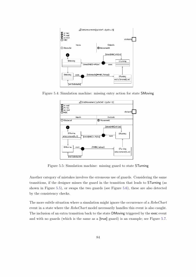
Figure 5.4: Simulation machine: missing entry action for state SMoving

Figure 5.5: Simulation machine: missing guard to state STurning

Another category of mistakes involves the erroneous use of guards. Considering the sametransitions, if the designer misses the guard in the transition that leads to STurning (asshown in Figure 5.5), or swaps the two guards (see Figure 5.6), these are also detectedby the consistency checks.

The more subtle situation where a simulation might ignore the occurrence of a RoboChartevent in a state where the RoboChart model necessarily handles this event is also caught.The inclusion of an extra transition back to the state DMoving triggered by the exec eventand with no guards (which is the same as a [true] guard) is an example; see Figure 5.7.

84

Figure 5.6: Simulation machine: swapping guards in transitions from DMoving

Figure 5.7: Simulation machine: possibly ignoring an obstacle occurrence

In this case, when a new cycle starts and an obstacle is detected, if the machine is in thestate DMoving, there is a nondeterminism between this new transition and the one thatleads to STurning. So the occurrence of an obstacle can be ignored, which is disallowedby the RoboChart machine when it is in the Moving state (see Figure 2.1).

Finally, we consider another subtle mistake where the wait(1) construct in the RoboChartmodel (see Figure 2.1) is not properly simulated. In the simulation in Figure 5.8, insteadof a junction with a single exec event from the state DMoving, as in the correct simula-tion (Figure 2.3), two transitions are used with exec guarded by the respective disjoint

85

Figure 5.8: Simulation machine: wrong cycle allocation

conditions on the occurrence (or the absence) of an obstacle. However, the guards arechecked in the current cycle, whereas the wait(1) in the RoboChart model imposes thatthese should be checked in the next cycle.

In summary, like the analysis of schedulability, soundness check of simulations with re-spect to design models can be very elaborate. Our reasoning framework allows (auto-matic) verification that can reveal subtle problems.

86

Chapter 6

Examples

We present below a few case studies. The first is a simple robot that performs a squaretrajectory, which shows how composite states, applications that terminate, and deadlinesmay be handled. A Transporter used in a swarm application, specified in [4], illustratessimulations with during actions. The Alpha Algorithm from [6] has multiple machinesthat can be independently simulated. Each of these examples is briefly discussed below,where we explore distinctive aspects of the simulation and conformance of the simulationmodel with respect to the RoboChart model.

6.1 Square

This case study involves a robot that performs a square trajectory, trying to avoid possibleobstacles.

6.1.1 RoboChart model

Here, we consider the RoboChart model from [18], reproduced here in Figure 6.1.

The initial transition leads to the state MovingForward; in this transition, the clock C isreset and the variable segment is initialised with 0; this variable is used to control thenumber of sides of the square that have been currently traversed. The execution flowterminates (reaches a final state) when the robot has covered all the sides of the square(segment == 4), in which case it communicates the event stop with deadline 0.

Since MovingForward is a composite state, entering in this state means executing its entryaction (moveForward with the constant parameter linear, for a linear motion) as well asthe entry action of the state Observing, namely, a call to enableCollisionDetection, as thereis an initial transition to this substate.

87

Figure 6.1: RoboChart: square trajectory state machine. The module contains a singlecontroller, which contains this machine.

The internal transition inside the state MovingForward happens when a collision is de-tected and the time guard since(C)<3 is satisfied, in which case the control moves tostate Collision. This transition causes the exit action of Observing to be executed, andthen the entry action of Collision. After the collision has been handled, an immediatetransition leads the control back to the substate Observing.

A transition can also be taken from the composite state MovingForward to Turning, when5 time units have passed; in this case the value of segment is incremented and the robotstarts an angular movement. This is interrupted after 2 time units, and the control goesback to MovingForward, when the clock is reset.

6.1.2 RoboSim model

A simulation model with a cycle value 1 is presented in Figure 6.2. The structure ofthe simulation could have mimicked that of the RoboChart model, since RoboSim also

88

Figure 6.2: RoboSim: square trajectory state machine

allows composite states. Instead, this simulation model linearises the RoboChart ma-chine, including only simple states. This might serve as a more concrete reference for animplementation, for instance. In the following section, we illustrate the use of compositestates in the simulation.

The actions from the initial state up to the state SObserving are similar to those inthe RoboChart model. We recall, nevertheless, that RoboSim does not allow deadlines.

89

Deadline constraints do not impact the RoboSimmodel itself, but rather they may requirethe definition of explicit assumptions on the environment to ensure that such constraintsare satisfied. After explaining the RoboSim model we further discuss the impact ofdeadlines in verification.

From the state DObserving, a number of transitions can be taken. If a collision is detectedwithin the allowed amount of time, the control flow transitions to EObserving and, then,immediately, to SCollision and to Waiting. This latter state allows two new cycles withoutany effect, except for time to pass, representing the wait(2) action in the RoboChartmodel, and then the control is transferred back to SObserving. Another transition fromDObserving is the one to state STurning, which immediately transitions to DTurning, fromwhich one transition allows to return to SMovingForward and another self-transition allowsthe change of cycle. Finally, a self-transition from DObserving has disjoint conditions tothe other two and allows the change of cycle.

There is a deadline 0 on the event stop in the transition from MovingForward to the finalstate. The simulation ensures that the relevant stop action is executed in the currentcycle by disallowing any transition triggered by exec.

This model is a provably correct simulation with respect to the RoboChart model in Fig-ure 6.1. In this case, no special treatment of the deadline is necessary for the verification.In general, however, particularly when deadlines are imposed on input events, it is nec-essary to define an environment assumption that ensures that the deadline constraintsare satisfied, namely, that the environment provides the input to satisfy the requireddeadline.

The asymmetry between inputs and outputs is because a deadline is an assumption onthe environment handled differently in RoboChart and RoboSim. In RoboChart, bothinputs and outputs require agreement of the environment to provide the input or ac-cept the output. In RoboSim, the environment is always ready to accept an output viaregisterWrite, as reflected in the model by buffering the outputs. On the other hand, theenvironment must provide the inputs: we can always read an input via registerRead , butit may not be ready as indicated by the boolean false.

In this case study, we have explored some variations of the RoboChart model. For exam-ple, we have considered different time constraints in the since and sinceEntry guards inthe RoboChart model, replacing 3 and 5 with 8 and 12 time units. We have also replacedwait(2) in state Collision with wait(4) and the guard SinceEntry(2) with SinceEntry(4). In

90

this case, we obtain a model that can be scheduled with a cycle at most 4, which is thegreatest common divisor of 4, 8 and 12. We have checked that cycle periods of size 1 and2 are also valid for that scenario.

As another variation, we have introduced nondeterminism in the RoboChart model, re-placing the wait(2) action in the entry action of Collision with the nondeterministic actionwait([2..4]), which defines a more flexible budget, with 2, 3 or 4 time units. The non-deterministic choice here determines the length of the cycles that are schedulable. Forinstance, for wait(3), a cycle of size 2 is not schedulable, as we need a common divisor ofthe time restrictions.

For these variations, we have also developed conforming simulation models.

6.2 Transporter

The transporter system proposes use of a swarm of small robots for moving an object toa specified goal. The robots move the object by pushing it.

The swarm is a fully distributed system: it involves no interaction among the robots.Our models capture the behaviour of a single robot; the swarm is formed of a number ofrobots with the behaviour specified here.

6.2.1 RoboChart model

Here we describe the RoboChart state machine of the Transporter system (see Figure 6.3).

In state Searching the robot searches for an object by calling searchObject and, onceit sees one, it transitions to state MovingToObject as triggered by the event objectSeen,which receives and assigns the estimated distance to variable distance. If the object isnearby, so the condition distance<close holds, and the object has been seen for less thanTa time units, then the state-machine transitions to state ClosingInOnObject. While instates MovingToObject and ClosingInOnObject if the object is lost for a certain amountof time Ta, then the robot initiates another search for the object by transitioning to stateSearching.

91

Figure 6.3: RoboChart state machine of the Transporter

In states MovingToObject and ClosingInOnObject we have the possibility to keep treat-ing the event objectSeen and updating the current distance, as long as, for stateMovingToObject the object has been last seen for less than Ta time units, and the dis-tance is greater than or equal to close, and similarly for state ClosingInObObject thedistance is greater than 0.

When the robot is close enough to the object, satisfying condition distance == 0,then it transitions from state ClosingInOnObject to Scanning and disables the objecttracking facility by calling disableObjectWatch. In state Scanning the robot initial-ized the variable goal to false, assuming that the goal is not visible until the firsttime event goalSeen takes place, and enables the capability to find the goal by callingenableGoalFinding.

Once the state Scanning has been entered, scanAndAlign is called, so that the robot canperform an alignment procedure, and a decision is taken S time units after entering the

92

state Scanning, to either transition to MovingAround if the goal is seen, or to transitionto Pushing if the goal is not seen. When taking this transition we initialize the variableneighbours, which keeps track of the number of nearby neighbours, to 2. This preventsthe transition from Pushing to Scanning from being triggered unless Tb time units havepassed since the most recent time, after having entered Pushing, where the number ofneighbours was observed to drop below 2, which can only be appropriately checked onceat least one reading of neighbourDetected has occurred. In state Pushing the robotfirst calls enabledObjectWatch to enable the facility to track the object, followed bythe call to enableNeighbourDetection to enable the facility to track neighbours. Oncestate Pushing is entered it finally calls the operation pushObject and can receive eventsobjectSeen and neighbourDetected.

The transition from Pushing to Evading takes place whenever the object has been lost forat least Tc time units. We specify this behaviour by taking into account the distance

to the object as given by objectSeen together with clock C. Whenever the distance

changes to being greater than 0, we reset clock C. The four possible cases are treated byseparate transitions whose guards are summarized below:

• objectSeen?d[distance==0/\d==0]: the object is seen at distance 0, so there isno need to change the existing value of distance.

• objectSeen?d[distance>0/\d==0]/distance=d: if the current distance is greaterthan 0, and the new distance is 0, then we just record the new value d in distance.

• objectSeen?d[distance>0/\d>0]: in every other case, we do not update the valueof distance.

The transition from Pushing to Scanning takes place whenever less than 2 neighbourshave been observed for at least Tb time units. We specify this behaviour using thevariable neighbours together with clock N, so that whenever the value drops below 2 wecount the time using clock N. We specify this using four transitions, whose guards aresummarized below:

• neighbourDetected?n[neighbours<2/\n<2]: the current count of neighbours isless than 2 and the new value being communicated is also less than 2, so there isno need to record a change.

93

• neighbourDetected?n[neighbours<2/\n>=2]/neighbours=n: the current countof neighbours is less than 2 and the new value n is greater than or equal to 2, sothere is a change to a situation in which at least 2 neighbours are around, so weupdated the value of neighbours to n.

• neighbourDetected?n[neighbours>=2/\n>=2]: in every other case in which thecount of current neighbours or the new value n is above 2 we do not update thevariable neighbours.

Before exiting state Pushing the capability to track the object and the neighbours isdisabled by calling disableObjectWatch and disableNeighbourDetection, respectively.

In general, the value of a since(C) condition for a clock C that has not been resetis arbitrary. We observe that in the case of the guard distance>0/\since(C)>=Tc,since(C)>=Tc has an appropriate value when distance>0 is true because clock C is resetprecisely when the value of distance becomes greater than 0. Similarly in the case ofthe guard neighbours<2/\since(N)>=Tb, since(N)>=Tb has an appropriate value whenneighbours<2 is true because clock N is reset precisely when the number of neighboursgoes below 2 as explained above.

In state Evading the robot evades the vicinity by calling the operation evade. Afterexactly Te time units it transitions to state Searching. Similarly, in state MovingAroundthe robot calls moveAroundObject which takes the robot around the object. After exactlyTd time units it transitions to state Searching.

We observe that the state-machine, and indeed the robotic controller, never terminates.This follows closely the description of the algorithm in the original paper. However inthe reported trials, robots could be stopped by a central controller that can ascertainwhether the object has been made contact with the goal, or after a certain amount oftime. We do not model that facility in this model.

6.2.2 RoboSim model

Figure 6.4 shows the RoboSim model of the algorithm, adding details about the opera-tional cycle, which refines our RoboChart model1.

1The interested reader can reproduce the verification of the simulation model. All CSP scripts areavailable at goo.gl/1so4uK.

94

Figure 6.4: RoboSim model of the Transporter

Rather than discussing the model of the simulation in detail, we focus here on somedistinctive aspects. We note, for instance, the use of composite states as a way to modelbehaviour in the presence of during actions in the design. For example, the model ofthe state MovingToObject is very similar in the RoboChart and RoboSim machines. InRoboSim, however, an additional transition with exec as trigger allows the change of cyclewhen no object is detected.

As another example, in the states Scanning and Pushing we observe the use of transitionsin the RoboSim model, to and from junctions, when contrasted with the several self-transitions in the respective states in the RoboChart model. This is a consequence ofthe need to control that the sensor readings for detecting the presence of an event mustnot be checked more than once in the same cycle. For instance, if $goalseen (in stateSearching) is checked to set the variable goal accordingly, which itself is used to enable

95

the transitions from this state, then it does not make sense to allow $goalseen to bechecked more than once in a same cycle. Another point we would like to emphasise isthat the RoboChart model of the transporter is nondeterministic, and the simulation isdeterministic. this case we have a refinement, not an equality between the RoboChartand RoboSim models.

6.3 Alpha Algorithm

Our third case study is the model of a single robot in a swarm acting under the AlphaAlgorithm [6]. This involves two machines: one specifying the robot movement, and theother, the communication with the other robots in the swarm.

6.3.1 RoboChart model

Figure 6.5 presents the RoboChartmodel of the more elaborateMovementmachine, whichis our focus here. A point of note is that, due to the compositional nature of our semantics,we can verify each machine separately.

The initial transition leads to the state MovementAndAvoidance. Here, a clock MBC isreset. Since the state MovementAndAvoidance is composite, entering it means executingthe entry action of the state Move, namely, move(lv,0); this operation is similar to thehomonymous ones of our running example and the Square example in Section 6.1, wherethe first parameter indicates the linear motion of the robot, and the second one theangular motion.

The transition from Move to Avoid happens when an obstacle is detected (represented bythe occurrence of the event obstacle) and no more than a certain amount of time, givenby (MB-360/av), has passed. Once in Avoid, its entry action is executed, and a period oftime must pass (as stated in the wait action) before returning to Move.

A transition can also be taken from MovementAndAvoidance to Turning if some amountof time equal or greater than MB time units has passed since the last clock reset. In thiscase, the clock MBC is reset. This means that the robot is required to turn after everyperiod of MB time units. Afterwards, the control goes back to MovementAndAvoidance.

96

Figure 6.5: RoboChart: Alpha Algorithm

6.3.2 RoboSim model

The simulation model for this example is presented in Figure 6.6. The simulation modelfor this example is presented in Figure 6.6. Its structure is similar to that of the RoboChartmodel, but it is also possible to notice some differences. As usual, we have included anextra state (here, DMove) in the composite state MovementAndAvoidance and an initialstate in Turning to control the cycle scheduling. In between the states MovementAn-

97

Figure 6.6: Simulation machine of the Alpha Algorithm in RoboSim

dAvoidance and Turning we have included the new state InfoNeighbours. This is necessarybecause, in RoboSim, input communications, such as $neighbours?n, are part of guards,and cannot happen in actions, since they are boolean expressions (possibly associatedwith an assignment to variables). We note that in the RoboChart model in Figure 6.5,the communication neighbours?n is a statement in the entry action of the state Turning.Finally, as already explained, the wait action is not available in RoboSim, so the occur-rences of wait in the states Avoid, RandomTurn and Turn180 are captured by countingcycles in the two Wait states.

We have proved that the simulation model is a correct implementation of the RoboChartmodel of the Movement machine2. During this verification, we have detected a schedu-

2The interested reader can reproduce the verification of the simulation model. All CSP scripts areavailable at goo.gl/fp8j2G.

98

lability issue in the RoboChart model. To avoid that two conflicting move operationshappen in the same cycle, the wait(1) action in Move (see Figure 6.5) had to be in-cluded. It can be difficult to get these right without proper verification support, as weare proposing here.

99

Chapter 7

Conclusions

We have presented here, RoboSim, a new notation for simulation of robots. We havedescribed a semantics for its core constructs. It uses CSP, but we envisage its extensionto use Circus [3], a process algebra that combines Z [24] and CSP, and includes timeconstructs [20]. Use of Circus and its UTP foundation will enable use of theorem provingas well as model checking. Work on probability is available in the UTP [25], but we willpursue an encoding of Markov decision processes in the UTP.

RoboChart itself misses support for modelling the environment and the robotic platformsin model detail. It is also in our plans to take inspiration from hybrid automata [9] toextend the notation, and from the UTP model of continuous variables [7] to define thesemantics.

100

Appendix A

Complete Metamodel

This appendix contains the metamodel for RoboSim as an extension of that for RoboChart,see Appendix B in [21]. It is specified in Ecore and formatted by the tool OCLinEcore.The syntax of the representation used in this appendix is available here.

A summary of the concepts of Ecore can be found here, and a tutorial is available here.

import ecore : ’http ://www.eclipse.org /emf /2002/ Ecore ’ ;import robochart : ’http ://www.robocalc.circus/text/RoboChart ’ ;

/** Controller*/class ControllerDef extends robochart :: ControllerDef{

property cycleDef : CycleDec [1]}class CycleDec extends robochart :: NamedExpression{

property cycle : robochart :: Variable [1] { composes };property cycleExp : robochart :: Expression [1] { composes };

}/** State Machine*/class StateMachineDef extends robochart :: StateMachineDef{

property cycleDef : CycleDec [1]property inputContext : Context [?]property outputContext : Context [?]

}/** Statement*/class PlatformCall extends robochart :: Statement

101

{property operation : robochart :: Operation [1];property args : robochart :: Expression [*|1] { ordered composes };

}/** Expression*/class InputCommunication extends robochart :: Expression{

property event : robochart :: Event [1];property variable : robochart :: Variable [?];property predicate : robochart :: Expression [?] { composes };property value : robochart :: Expression [?] { composes };

}class PlatformVariable extends robochart :: Expression{

property variable : robochart :: Variable [1];}/** Module*/class Module extends robochart :: Module{

property cycleDef : CycleDec [1]}

102

Bibliography

[1] R. H. Bordini, J. F. Hübner, and M. Wooldridge. Programming Multi-Agent Systemsin AgentSpeak using Jason. John Wiley & Sons, 2007.

[2] S. G. Brunner, F. Steinmetz, R. Belder, and A. Domel. Rafcon: A graphical toolfor engineering complex, robotic tasks. In IEEE/RSJ International Conference onIntelligent Robots and Systems, pages 3283–3290, 2016.

[3] A. L. C. Cavalcanti, A. C. A. Sampaio, and J. C. P. Woodcock. A RefinementStrategy for Circus. Formal Aspects of Computing, 15(2 - 3):146–181, 2003.

[4] J. Chen, M. Gauci, and R. Groß. A strategy for transporting tall objects witha swarm of miniature mobile robots. In 2013 IEEE International Conference onRobotics and Automation, pages 863–869, May 2013.

[5] S. Dhouib, S. Kchir, S. Stinckwich, T. Ziadi, and M. Ziane. Simulation, Modeling,and Programming for Autonomous Robots, chapter RobotML, a Domain-SpecificLanguage to Design, Simulate and Deploy Robotic Applications, pages 149–160.Springer, 2012.

[6] C. Dixon, A. F. T. Winfield, M. Fisher, and C. Zeng. Towards temporal verificationof swarm robotic systems. Robotics and Autonomous Systems, 60(11):1429–1441,2012.

[7] S. Foster, B. Thiele, A. L. C. Cavalcanti, and J. C. P. Woodcock. Towards a UTPsemantics for Modelica. In Unifying Theories of Programming, Lecture Notes inComputer Science. Springer, 2016.

[8] T. Gibson-Robinson, P. Armstrong, A. Boulgakov, and A. W. Roscoe. FDR3 - AModern Refinement Checker for CSP. In Tools and Algorithms for the Constructionand Analysis of Systems, pages 187–201, 2014.

[9] T. A. Henzinger. The theory of hybrid automata. In 11th Annual IEEE Symposiumon Logic in Computer Science, pages 278–292, 1996.

103

[10] C. A. R. Hoare and He Jifeng. Unifying Theories of Programming. Prentice-Hall,1998.

[11] S. Luke, C. Cioffi-Revilla, L. Panait, K. Sullivan, and G. Balan. Mason: A multiagentsimulation environment. Simulation, 81(7):517–527, 2005.

[12] The MathWorks,Inc. Simulink. www.mathworks.com/products/simulink.

[13] The MathWorks,Inc. Stateflow and Stateflow Coder 7 User’s Guide.www.mathworks.com/products.

[14] A. Miyazawa, P. Ribeiro, W. Li, A. L. C. Cavalcanti, and J. Timmis. Automaticproperty checking of robotic applications. In IEEE/RSJ International Conferenceon Intelligent Robots and Systems, pages 3869–3876, 2017.

[15] M. V. M. Oliveira, P. Antonino, R. Ramos, A. C. A. Sampaio, A. C. Mota, andA. W. Roscoe. Rigorous development of component-based systems using componentmetadata and patterns. Formal Aspects of Computing, 28(6):937–1004, 2016.

[16] I. Pembeci, H. Nilsson, and G. Hager. Functional reactive robotics: An exercise inprincipled integration of domain-specific languages. In 4th ACM SIGPLAN Inter-national Conference on Principles and Practice of Declarative Programming, pages168–179. ACM, 2002.

[17] C. Pinciroli, V. Trianni, R. O’Grady, G. Pini, A. Brutschy, M. Brambilla, N. Math-ews, E. Ferrante, G. Di Caro, F. Ducatelle, M. Birattari, L. M. Gambardella, andM. Dorigo. ARGoS: a modular, parallel, multi-engine simulator for multi-robotsystems. Swarm Intelligence, 6(4):271–295, 2012.

[18] P. Ribeiro, A. Miyazawa, W. Li, A. L. C. Cavalcanti, and J. Timmis. Modelling andverification of timed robotic controllers. In N. Polikarpova and S. Schneider, editors,Integrated Formal Methods, pages 18–33. Springer, 2017.

[19] A. W. Roscoe. Understanding Concurrent Systems. Texts in Computer Science.Springer, 2011.

[20] A. Sherif, A. L. C. Cavalcanti, J. He, and A. C. A. Sampaio. A process algebraicframework for specification and validation of real-time systems. Formal Aspects ofComputing, 22(2):153–191, 2010.

104

[21] University of York. RoboChart Reference Manual.www.cs.york.ac.uk/circus/RoboCalc/robotool/.

[22] M. Wachter, S. Ottenhaus, M. Krohnert, , N. Vahrenkamp, and T. Asfour. Thearmarx statechart concept: Graphical programing of robot behavior. Frontiers inRobotics and AI, 3:33, 2016.

[23] U. Wilensky and W. Rand. An Introduction to Agent-Based Modeling – ModelingNatural, Social, and Engineered Complex Systems with NetLogo. MIT Press, 2015.

[24] J. C. P. Woodcock and J. Davies. Using Z—Specification, Refinement, and Proof.Prentice-Hall, 1996.

[25] H. Zhu, J. W. Sanders, He Jifeng, and S. Qin. Denotational Semantics for a Prob-abilistic Timed Shared-Variable Language. In B. Wolff, M.-C. Gaudel, and A. Fe-liachi, editors, Unifying Theories of Programming, volume 7681 of Lecture Notes inComputer Science, pages 224–247. Springer, 2013.

105

Index of Semantic Rules

In this index you’ll find the list of semantic functions in alphabetic order, and page where theyare defined.

allConstants, 66allLocalVariables, 65allTransitions, 66allVariables, 65alphaClockReset, 54

And (timed), 55CallExp (timed), 55ClockExp (timed), 58Equals (timed), 57GreaterOrEqual (timed), 57GreaterThan (timed), 56Iff (timed), 56Implies (timed), 56LessOrEqual (timed), 57LessThan (timed), 57Not (timed), 55Or (timed), 56ParExp (timed), 54

alphaClockResetCallArgs (timed), 55

behaviours, 49buffer, 48

C (Controller), 43clockResets, 54clockVariables, 53compileWC (timed), 70–75composeControllers, 42composeMachines, 44composeStates, 67

constInit, 68cycle, 46cycleComp, 44

Expr (Expression), 58And Expression, 58Array Expression, 58Boolean Expression, 59Call Expression, 59Concatenation Expression, 59Division Expression, 60Equals Expression, 60Greater or Equal Expression, 60Greater Than Expression, 61If and Only If Expression, 61Implies Expression, 61Integer Expression, 61Less or Equal Expression, 62Less Than Expression, 62Minus Expression, 62Modulus Expression, 62Multiplication Expression, 63Negation Expression, 63Not Equal Expression, 60Not Expression, 63Or Expression, 63Parenthesised Expression, 64Plus Expression, 64Range Expression, 64

106

Sequence Expression, 64Set Expression, 65Tuple Expression, 65

flowEvents, 68

getsetChannels, 52

M (Module), 40memoryComp, 42memoryTransition, 51

operationCall, 53

requiredVariables, 66

restrictedState, 67

S (State)Final State, 52

StateMachineDef, 45states, 68stmClocks (timed), 47, 54stmMemory, 50

transitionsFrom, 68trigEvents, 52trigger, 51triggerEvent, 66triggerForMemory, 53

107

Index of Calls to Semantic Rules

In this index you’ll find the location of call to the semantic rules. For each call of a semanticfunction, the page number superscripted with the usage index is provided. The index of the callis unique with respect to the semantic function, and also shown superscripted in the call location.

allConstants , 401, 412, 503, 504,525, 526, 687

allLocalVariables , 501

allTransitions , 451, 462, 503, 514,525, 676, 677

allVariables , 521, 522

alphaClockReset (timed) , 471, 542,543, 544, 555, 556, 557, 558,5610, 5611, 5612, 5613, 5614,5615, 5616, 569, 5717, 5718,5719, 5720, 5721, 5722, 5723,5724

alphaClockResetCallArgs (timed) , 551,552

behaviours , 451, 482

buffer , 451

clockResets , 451, 452, 523

clockVariables , 501

compileWC (timed) , 471, 542

composeControllers , 401, 422

composeMachines , 431

composeStates , 491, 672

constInit , 411, 422

cycle , 451

cycleComp , 401, 412, 433, 434, 445

Expr (Expression) , 511, 582, 583,584, 585, 5910, 596, 597,598, 599, 6011, 6012, 6013,6014, 6015, 6016, 6017, 6018,6119, 6120, 6121, 6122, 6123,6124, 6225, 6226, 6227, 6228,6229, 6230, 6231, 6232, 6333,6334, 6335, 6336, 6337, 6338,6439, 6440, 6441, 6442, 6443,6444, 6545, 6546, 7047, 7048,7049, 7050, 7151, 7152, 7153,7154, 7255, 7256, 7257, 7258,7359, 7360, 7361, 7362, 7463,7464, 7465, 7466, 7567, 7568,7569, 7570

flowEvents , 671, 672

getsetChannels , 451, 452, 523

memoryComp , 401, 412, 413, 434

memoryTransition , 501, 512, 513

restrictedState , 671, 672

states , 681

stmClocks (timed) , 451, 462

stmMemory , 451

transitionsFrom , 671

108

trigEvents , 451, 452, 523

triggerEvent , 471

triggerEvent (timed) , 451, 472, 523,544, 7010, 7011, 7012, 705,706, 707, 708, 709, 7113,7114, 7115, 7116, 7117, 7118,7119, 7120, 7221, 7222, 7223,

7224, 7225, 7226, 7227, 7228,7329, 7330, 7331, 7332, 7333,7334, 7335, 7336, 7437, 7438,7439, 7440, 7441, 7442, 7543,7544, 7545, 7546, 7547, 7548

triggerForMemory , 511, 512

109