road extraction from lidar data in …asprs.org/a/publications/proceedings/sandiego2010/san...asprs...

ASPRS 2010 Annual Conference San Diego, California April 26-30, 2010

ROAD EXTRACTION FROM LIDAR DATA IN RESIDENTIAL AND COMMERCIAL AREAS OF ONEIDA COUNTY, NEW YORK

Yue Zuo, Graduate Student ([email protected])

Lindi Quackenbush, Assistant Professor ([email protected]) State University of New York College of Environmental Science and Forestry

Syracuse, NY 13210

ABSTRACT Since roads play an important role in many application areas, up-to-date road databases are critical. Automated road extraction using many different types of remote sensing data has been explored. Recently, lidar data has proven advantageous for road extraction and researchers have extracted roads from lidar data alone as well as fused with passive imagery. This paper considers techniques to extract roads from lidar data exclusively and explores the impact of land use on the accuracy of the derived road network. To support this goal, roads were extracted from lidar data for six study sites—three residential and three commercial—within Oneida County, NY. The accuracy of generated results was computed and comparison tests were performed. These results showed high levels of accuracy for the raster road cluster delineation, with lower accuracy for the vector centerlines. The comparative analysis showed that land use was a factor in road delineation accuracy for both the raster and vector stages of analysis.

INTRODUCTION The Problem

Roads have long been important for development and prosperity and are essential for many applications related to transportation, water resource management, and wildlife management. Research on automated road extraction has been applied to many different types of remote sensing data over recent decades. Development during this period has gone from low resolution to high resolution image data, and more recently has extended into data fusion. Lidar data, which contains accurate elevation information, has proven useful for road extraction because of the ability to separate roads from other artificial objects such as buildings. Fusing datasets, such as lidar and high spatial resolution imagery, has proven theoretically advantageous, but is frequently cost-prohibitive to apply practically. Prior research has shown that lidar data is useful for generating vector road networks that are suitable for incorporation in GIS databases. Aside from high quality elevation information, lidar intensity data provides good separability for ground materials, especially for road vs. grass and road vs. tree (Song et al., 2002). In this paper, we aim to extract roads from lidar data and to explore the impact of land use on the accuracy of the derived road network. The project has two fundamental objectives: (1) extract roads from lidar data in Oneida County, NY; and (2) compare the extraction accuracy for two different types of land use—i.e., residential and commercial—within three urban areas of Oneida County, NY. Both objectives will be addressed in raster and vector based stages.

Road Extraction Approaches

Road extraction is typically divided into two main steps: (1) define raster road clusters, and (2) generate the vector road network. This section presents some of the methodology used to address each of these steps. The first step in road delineation typically involves classification to identify candidate raster road clusters before vectorization is performed (Clode et al., 2007); many classification techniques have been used to generate a binary road network. Agouris et al. (2001) applied an unsupervised classification and determined roads through a k-medians algorithm. Zhang (2006) chose a simple k-means clustering algorithm for image segmentation and used a fuzzy logic classifier to identify road clusters. Object-based classification was used by Tiwari et al. (2009) for road extraction. Im et al. (2007) developed an automatic calibration model for binary change detection of land use. Their automatic calibration model uses an exhaustive search technique with a stratified sampling design of the research space to determine optimal thresholds for each input layer. The automatic calibration model can be used to find optimal thresholds for lidar-derived height and intensity to identify a preliminary raster road network.

After defining potential road strips, features that are spectrally similar to roads such as parking lots are likely to negatively impact classification accuracy, and most researchers further process the derived raster road strips to remove noise and correct errors. From our review of the literature, we identified three useful refinement methods:


local density, angular texture signature, and mathematical morphology. The local point density method was presented by Clode et al. (2004). This method examines pixels within a local neighborhood (e.g., 3×3 window) to identify the local density of road points within the binary road layer. The local point density for a pixel in the middle of a road is generally higher than that of a pixel lying on the edge of a road. Due to blockage caused by features such as vehicles and overhanging trees, lidar points are likely not to be equally distributed. The goal of applying the local point density method is to preserve all lidar points that are expected to be road points and eliminate noise.

The angular texture signature (ATS) was developed for road extraction from high resolution panchromatic imagery and is described in Haverkamp (2002) and Gibson (2003). For each pixel in an image, the ATS considers a set of n rectangles in n directions (Zhang and Couloigner, 2006a). The implementation of the ATS for road extraction commonly utilizes a binary image where pixels are classified as road vs. non-road. The ratio of the number of road pixels to the total number of pixels is computed for each rectangle. The ATS value at each pixel is defined using the set of n values. Two common metrics derived are the ATS-mean and the ATS-compactness. ATS-mean is defined as the mean of all the ATS values for n directions. It indicates the average percentage of road pixels surrounding the current pixel within the rectangular region. Given the non-linear nature of a parking lot, pixels within a parking lot typically have a larger ATS-mean than road pixels. ATS-compactness is formed by plotting the values from each ATS direction for a pixel and connecting the points to create a polygon. ATS-compactness considers the area (A) and perimeter (P) of the ATS polygon. Points along linear features—e.g., roads—tend to generate lower ATS compactness values compared to points in large blocks—e.g., parking lots.

Mathematical morphology has proven useful in feature extraction (Quackenbush, 2004), and has been successfully used by many researchers in road extraction (Zhang et al, 1999; Amini et al., 2002; Chanussot et al., 1999). The most common operators in mathematical morphology are dilation and erosion. Dilation is used for expanding features in an image and closing any gaps, while erosion shrinks image features and eliminates small features. Since mathematical morphology methods are useful for segmentation and image enhancement, it is commonly applied to enhancing road network extraction.

Having generated and refined raster road clusters, the extraction of vector centerlines from the clusters is challenging and many methods have been considered. Common line detection methods such as the Hough transform (Duda and Hart, 1972) have limitations in high resolution imagery where the peak of the Hough transform corresponds to the diagonal of a road segment in the image (Clode et al., 2004). The Radon transform provides another alternate method for line detection. The Radon transform was first introduced by Radon (1917) and projects image intensity along a radial line oriented at a specific angle. The mathematical definition of the Radon transform is described in detail by Murphy (1986). The Radon transform converts images containing lines into a domain of possible line parameters (Zhang and Couloigner, 2007). For a two-dimensional image, the computation of its Radon transform considers projections across the image at varying orientations and offsets (Murphy, 1986). The Radon transform contains bright peaks corresponding to each line in the image thus the problem of line detection is reduced to detecting the peaks in the transform domain (Zhang and Couloigner, 2007). An important property of the Radon transform is the ability to extract lines (curves in general) from very noisy images (Toft, 1996). To avoid the problem with diagonal line detection and improve centerline detection accuracy, an iterative and localized Radon transform was developed by Zhang (2006).

STUDY AREA

The study area selected for this project was in Oneida County in central New York State. Three urban sites with both residential and commercial areas were identified in the county within the cities of Rome, Utica, and Sherrill. Most of the other parts of Oneida County within the lidar data collection area are rural and contain a very low road density. For each urban center, one residential area and one commercial area were selected.

Figure 1 shows digital orthoimagery of the six study areas within the three urban centers. The size of each study area is 1.5 km × 1.5 km.


Figure 1. First row: Residential areas in Sherrill, Utica, and Rome; Second row: Commercial areas in Sherrill, Utica, and Rome.

DATA

Two sources of data were utilized in this project: lidar data and digital orthoimagery. The parameters of these data sets are summarized in Table 1. The orthoimagery was used as a visualization aid to guide accuracy assessment and sample point collection. Vector reference road data were generated from the orthoimagery and verified through ground surveys. The bare earth surface was generated from the raw lidar data by Sanborn Map Company. This dataset contains ground surface elevation information for the Oneida County study sites. The lidar point data in LAS format was the first return data containing elevation and intensity information for each lidar point. Each point in the dataset had four variables: x, y, z, i, where x, y, and z are the three dimension coordinates and i is the intensity value for each point.

Table 1. Summary of data utilized

Dataset Format CoordinateSystem Datum Spatial

Sampling Acquisition

Date Source

Orthoimagery JPEG2000 State Plane NAD1983 1ft April 2008 NYS GIS Clearinghouse Bare earth data ESRI Terrain UTM NAD1983 1m April 2008 Sanborn Map Company

Lidar point cloud LAS UTM NAD1983 2 points/m2 April 2008 Sanborn Map Company

RASTER ROAD CLUSTER DEFINITION

As mentioned in the objectives, road delineation was performed in two stages: (1) defining raster road clusters, and (2) generating the vector road network. For defining the raster road clusters, we identified potential road strips within flat, impervious regions and then further processed this to remove noise and correct errors. To extract the


raster road clusters, we used an automatic calibration model (Im et al. 2007) to find the optimal threshold of the height and intensity layers generated from the lidar point cloud and bare earth data. After obtaining the binary road strips, we used several methods to remove noise and correct errors.

Preprocessing

Preprocessing of the original datasets was needed to utilize the automatic calibration model. The ESRI Terrain file supplied was converted to a raster grid to create a digital terrain model (DTM) for each study area. This DTM data contained elevation information of the bare earth surface without the influence of ground feature height. Three other layers were generated during the preprocessing: (1) a raster height layer containing feature height information, (2) a raster intensity layer containing lidar intensity information, and (3) a reference point layer containing road and non-road labels.

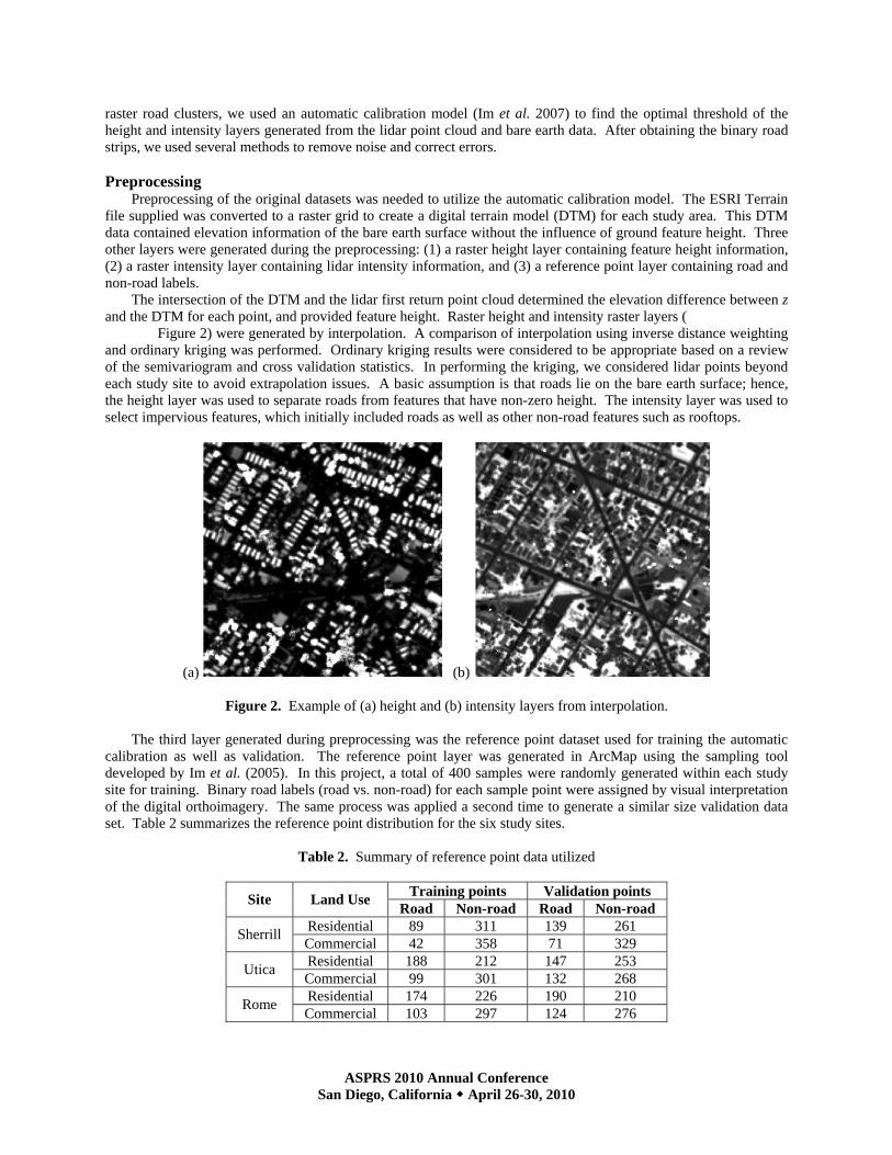
The intersection of the DTM and the lidar first return point cloud determined the elevation difference between z and the DTM for each point, and provided feature height. Raster height and intensity raster layers (

Figure 2) were generated by interpolation. A comparison of interpolation using inverse distance weighting and ordinary kriging was performed. Ordinary kriging results were considered to be appropriate based on a review of the semivariogram and cross validation statistics. In performing the kriging, we considered lidar points beyond each study site to avoid extrapolation issues. A basic assumption is that roads lie on the bare earth surface; hence, the height layer was used to separate roads from features that have non-zero height. The intensity layer was used to select impervious features, which initially included roads as well as other non-road features such as rooftops.

(a) (b)

Figure 2. Example of (a) height and (b) intensity layers from interpolation.

The third layer generated during preprocessing was the reference point dataset used for training the automatic calibration as well as validation. The reference point layer was generated in ArcMap using the sampling tool developed by Im et al. (2005). In this project, a total of 400 samples were randomly generated within each study site for training. Binary road labels (road vs. non-road) for each sample point were assigned by visual interpretation of the digital orthoimagery. The same process was applied a second time to generate a similar size validation data set. Table 2 summarizes the reference point distribution for the six study sites.

Table 2. Summary of reference point data utilized

Training points Validation points Site Land Use Road Non-road Road Non-road

Residential 89 311 139 261 Sherrill Commercial 42 358 71 329 Residential 188 212 147 253 Utica Commercial 99 301 132 268 Residential 174 226 190 210 Rome Commercial 103 297 124 276


Delineating Potential Road Strips Delineation of potential raster road strips considered two components: (1) identifying road-level features; and

(2) selecting impervious features. The first component was based around the assumption that roads generally lie on or near the bare earth surface, with the exception of elevated roads, bridges, and tunnels. Therefore, we sought to establish an optimal height threshold to select all the road-level features and remove all features with non-zero height (e.g., buildings and trees). The second component involved selection of impervious features if their intensity values were between the acceptable ranges for the type of road material being detected (i.e., bitumen). By searching for a particular intensity range it was possible to identify impervious features with similar characteristics, including both road and other non-road features.

While thresholds can be established manually, our study applied an automatic calibration model (Im et al. 2007) to delineate potential road strips. The inputs into the automatic calibration model were the height and intensity layers generated during preprocessing and the binary (road vs. non-road) training point information. We obtained all potential road points by searching the attribute table of the lidar point cloud to identify points that met the optimal thresholds attained for road-level and impervious features. The output of this processing removed many of the non-road areas, e.g., buildings and pervious regions, but still contained significant noise and errors.

Removing Noise and Correct Errors

The identification of potential road strips is negatively impacted by the presence of parking lots and other flat features that are spectrally similar to roads. To identify the final raster road clusters and gain optimal accuracy, it was necessary to eliminate noise and correct errors. In our study, we used three methods for noise reduction of the raster layer: local point density, angular texture signature, and mathematical morphology.

Local point density. We applied a kernel density function with a search radius of 5 m (half the average road width) to calculate the local density of lidar points within the potential road strips derived from the initial processing. A raster density map was generated using the kernel density function in ArcMap and the optimal density threshold for roads was determined by again applying an automatic calibration model. Through appropriate threshold selection, most of the points along the road edge were maintained as road elements, while points that did not satisfy the minimum local density were removed.

Angular texture signature. The local density function left clusters of non-road pixels, thus ATS methods were used to further refine the raster layer. In order to apply the ATS methods on a classified binary image, Zhang and Couloigner (2006a) defined three different ATS descriptors: ATS-mean, ATS-compactness, and ATS-eccentricity. Since the ATS-eccentricity tended to show high values only on the boundary of each parking lot, it was considered unsuitable for reducing parking lot errors. Therefore, to remove parking lots from the binary road map, we computed ATS-mean and ATS-compactness in our study. Several parameter combinations were tested, with the best results attained for ATS values computed based on 18 rectangles with a size of 10 × 40 m for each rectangle. There were several differences in the two indicators for the linear roads—moderate ATS values—compared to the larger parking lots—high ATS values. We compared the results of the ATS-mean and ATS-compactness measures based on several thresholds. While most of the parking lots were successfully removed using the ATS-mean, this measure was sensitive to neighboring pixels, which made it difficult to threshold. As a result, we used the ATS-compactness to remove the remaining parking lots and a few large driveways from our binary road map.

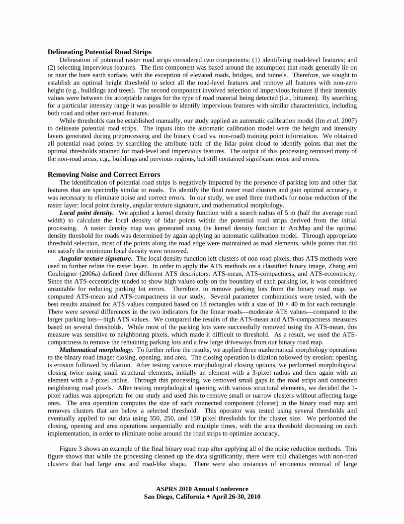
Mathematical morphology. To further refine the results, we applied three mathematical morphology operations to the binary road image: closing, opening, and area. The closing operation is dilation followed by erosion; opening is erosion followed by dilation. After testing various morphological closing options, we performed morphological closing twice using small structural elements, initially an element with a 3-pixel radius and then again with an element with a 2-pixel radius. Through this processing, we removed small gaps in the road strips and connected neighboring road pixels. After testing morphological opening with various structural elements, we decided the 1-pixel radius was appropriate for our study and used this to remove small or narrow clusters without affecting large ones. The area operation computes the size of each connected component (cluster) in the binary road map and removes clusters that are below a selected threshold. This operator was tested using several thresholds and eventually applied to our data using 350, 250, and 150 pixel thresholds for the cluster size. We performed the closing, opening and area operations sequentially and multiple times, with the area threshold decreasing on each implementation, in order to eliminate noise around the road strips to optimize accuracy.

Figure 3 shows an example of the final binary road map after applying all of the noise reduction methods. This

figure shows that while the processing cleaned up the data significantly, there were still challenges with non-road clusters that had large area and road-like shape. There were also instances of erroneous removal of large


intersections (e.g., top, center of the figure); further correction of such errors was considered during the vector processing.

Figure 3. Example of final binary raster road map after noise reduction.

GENERATE VECTOR ROAD NETWORK

Defining the raster road clusters accomplished half of the first project goal. This section summarizes the procedures used to achieve the second main component of this goal: generating the vector road network. This component involved road centerline extraction to convert the identified raster road clusters into meaningful road lines to format the final vector road network. For this project, with the input simplified to binary imagery, the Radon transform was appropriate and relatively easy to implement. Therefore, in our project, we applied a local Radon transform and then connected road centerline components to generate the final vector road network for each study site.

Radon Transform Localization

In previous work, researchers have derived road centerlines using the Radon transform. While the transform works well in simple scenarios, it struggles with larger image sizes and complex road networks that include segments with a variety of lengths. When an image contains multiple road lengths, the Radon transform detects long road components and ignores the shorter road segments. To solve this problem, Zhang and Couloigner (2006b) developed and tested three approaches to partitioning input images in order to localize the Radon transform. Based on their test results, Zhang and Couloigner (2006b) found that the gliding-box approach had better overall performance and lower computational load than the other two methods they tested. Therefore, we used the gliding-box approach to localize the Radon transform on our study sites.

Following initial testing with various window sizes, our implementation of the gliding-box approach used a window with a size of 100 × 100 pixels, and a 100 pixel increment. Because the size of each study site in our project was 1.5 × 1.5 km, the selection of parameters subset the input image into 225 regions. Based on this image subdivision, long roads were split by the moving window, thus reducing complexity and generating road components in each subset with more consistent length. This enabled extraction of a series of short centerline segments, which were linked in a later step.

We applied a Radon transform to each subset of the binary raster road image using tools within the MATLAB program (MathWorks, 2008). Each bright peak in the radon graph indicates a road component. To correctly estimate the line parameters, we used the robust peak selection approach presented by Zhang (2006). In this approach, the radon peak region, which was defined as the connected elements that have a value larger than 85% of the peak value, was used instead of single peak. We used the centroid of the peak region to estimate the line parameters and detect the road centerline for each road component.


Endpoint Generation The output from the Radon analysis is a series of continuous, and infinitely long, lines. However, this is not a

true representation of a road network, i.e., roads are made up of line segments that have defined endpoints. Since the Radon transform generates continuous lines, it does not provide any information about the endpoints of a given line segment, and in many cases, extends lines across places where there should be a break. We identified road segment endpoints by overlaying the detected centerlines on the binary road image. After overlaying the centerline on the binary road image, we found that some vector features diverged from the raster clusters, e.g. with lines crossing in the middle of the raster road strips rather than at the end, which resulted in omission of the extracted centerline. The reason for this problem was that some line parameters, determined from the Radon transform were biased based on the peak selection. To solve this problem, we used a buffer method for endpoint generation. We first made a buffer with a width of five pixels around each continuous centerline. The buffer width was selected to be at least half the width of the widest road in the study sites. Then, based on the line direction information derived in the Radon transform, for each pixel along the centerline in the binary road image we searched for road pixels within the buffer perpendicular to the centerline. For a particular pixel, if there was no road pixel that could be found within the buffer in the direction perpendicular to centerline, then the endpoint was recorded in the location of this pixel. Having found all the endpoints; the road segments constructed by these endpoints had approximately the same length as that of the road clusters. Network Formation

After reuniting all the image subsets we obtained a set of separate road centerlines constructed by endpoints for each study site. We then connected centerlines by fusing gaps and removing short segments that were likely to be non-road components. Gaps in the road centerlines may have been caused by the localization of the moving window in the Radon transform, through intersection elimination during the ATS processing, or from the exclusion of elevated roads and bridges in the road-level feature identification phase. We computed the distance between unconnected endpoints, and fused nearby points to close gaps. We also calculated the distance between connected endpoints and removed short segments that were likely non-road components. From this processing we obtained a vector road network for each site.

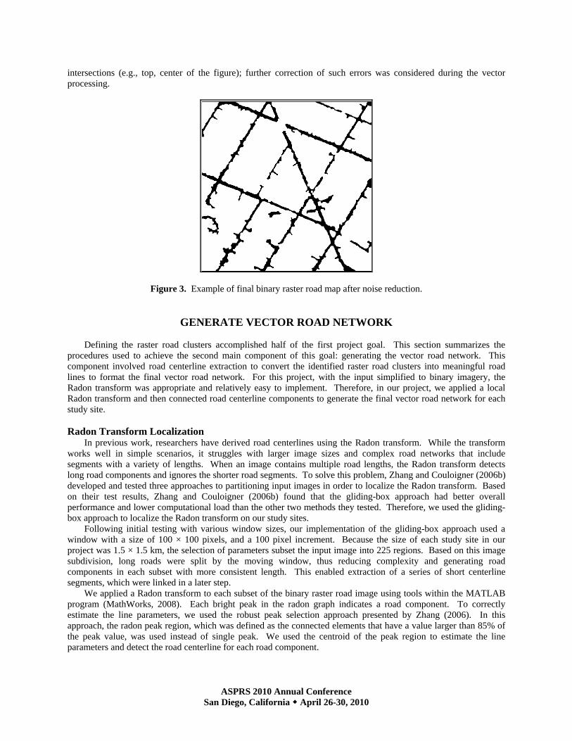
Figure 4 shows an example of the result of vector processing and error correction.

Figure 4. Example of final road segment centerlines constructed through vector processing.

VALIDATION AND DISCUSSION

Validation work was performed to assess the results of the raster road classification and the vectorization of the

extracted road network. The assessment of our study also compared the results in residential and commercial areas to assess the impact of land use on accuracy.


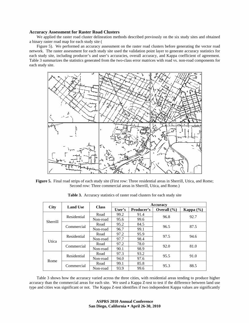
Accuracy Assessment for Raster Road Clusters We applied the raster road cluster delineation methods described previously on the six study sites and obtained

a binary raster road map for each study site ( Figure 5). We performed an accuracy assessment on the raster road clusters before generating the vector road

network. The raster assessment for each study site used the validation point layer to generate accuracy statistics for each study site, including producer’s and user’s accuracies, overall accuracy, and Kappa coefficient of agreement. Table 3 summarizes the statistics generated from the two-class error matrices with road vs. non-road components for each study site.

Figure 5. Final road strips of each study site (First row: Three residential areas in Sherrill, Utica, and Rome; Second row: Three commercial areas in Sherrill, Utica, and Rome.)

Table 3. Accuracy statistics of raster road clusters for each study site

Accuracy City Land Use Class User’s Producer’s Overall (%) Kappa (%)

Road 99.2 91.4 Residential Non-road 95.6 99.6 96.8 92.7

Road 95.2 84.5 Sherrill Commercial Non-road 96.7 99.1 96.5 87.5


Road 97.2 78.0 Utica Commercial Non-road 90.1 98.9 92.0 81.0


Road 99.1 85.8 Rome Commercial Non-road 93.9 99.6 95.3 88.5

Table 3 shows how the accuracy varied across the three cities, with residential areas tending to produce higher

accuracy than the commercial areas for each site. We used a Kappa Z-test to test if the difference between land use type and cities was significant or not. The Kappa Z-test identifies if two independent Kappa values are significantly


different (Congalton and Green, 2009). With a null hypothesis of equal Kappa values, the Z-statistic is defined in Equation 1, where k1 and k2, are the two Kappa values and Var(k1) and Var(k2) are their variances. The null hypothesis is rejected if the Z-statistic is greater than a critical value (1.96 for a 95% confidence level). Table 4 and Table 5 demonstrate the results of the Kappa Z-tests for pairwise comparison of land use and city, respectively.

)()( 21

21

kVarkVarkk

Z+

−=

Equation 1

Table 4. Kappa Z-test between residential and commercial areas for each city

Land Use Comparison City Kappa Z-test Statistic Sherrill 4.12 Utica 8.77 Residential vs. Commercial Rome 1.69

Table 5. Kappa Z-test between each pair of cities for the residential and the commercial area

Land Use City Comparison Kappa Z-test Statistic

Sherrill vs. Utica 1.62 Utica vs. Rome 2.81 Residential

Sherrill vs. Rome 1.28 Sherrill vs. Utica 3.99 Utica vs. Rome 4.38 Commercial

Sherrill vs. Rome 0.72 From Table 4, we can see that the comparison of land use in both Sherrill and Utica has a Z-value larger than

1.96, which indicates that there is a significant difference in accuracy between residential and commercial areas. Although Rome has a Z-value lower than 1.96, it is close to this threshold. Based on our methods for road extraction, it appears that the raster extraction accuracies are impacted by the type of land use. This is likely because the residential areas in the study site were similar to those in many parts of the United States in that they are largely laid out in a regular grid and have few parking lots. The commercial areas tended to have a much more complex road network, including large parking lots, leading to the lower accuracy levels. In many cases, parked cars divided parking lots into multiple pieces that were then erroneously identified as separate road segments. While the ATS methodology worked well for identifying empty parking lots, it was less effective for occupied lots. Table 5 demonstrates that our road extraction accuracies are slightly different among the three urban centers. The reason for the accuracy difference might be the variety of road complexity and the degree of commercialized development.

Accuracy Assessment for Vector Road Network

Accuracy assessment of the vector road network followed the evaluation method proposed by Heipke et al. (1997) comparing the extracted road network with a reference road network. The validation was processed in two steps: (1) matching the extracted road network to the ground survey data; and (2) calculation of accuracy. Heipke et al. (1997) suggested using a buffer approximately half the road width in order to determine the match between the extracted and reference data. The use of a buffer was based on the assumption that a road is extracted correctly if the road axis lies between the roadsides. In our project, this buffer was generated with a distance of 4 m, which was approximately half the typical road width in our study sites.

The quality measures of completeness, correctness, and quality as defined in Heipke et al. (1997) were examined to evaluate the extraction results. Completeness is the ratio of the reference road data that matches extracted road data to the total length of the reference road network. It indicates the percentage of reference data that is explained by the extracted data. Correctness is the ratio of extracted roads that match reference roads to the total length of the extracted road network. This indicates the percentage of correctly extracted road data. Quality is an overall accuracy measure and is computed as the ratio of the length of matched extraction to the sum of the length extracted plus the length of any unmatched reference. All the measures have an optimum value of 100%.


Assessment of the vector road network also compared the two different types of land use, i.e., contrasting the residential vs. commercial sites.

Figure 6 illustrates the vector road network generated for each of the six study sites. Table 6 summarizes the assessment of the vector road extraction and demonstrates the difference in accuracy between the two types of land use. Regardless which measure or city was considered, the accuracy for the commercial sites was generally lower than that for the residential sites.

Figure 6. Final road network for each study site overlaid on digital orthophotography (First row: Residential areas in Sherrill, Utica, and Rome; Second row: Commercial areas in Sherrill, Utica, and Rome.).

Table 6. Accuracy assessment results contrasting each type of land use for the three study sites

Land Use City Completeness (%) Correctness (%) Quality (%)

Sherrill 83.7 84.7 72.5 Utica 89.3 88.4 79.8 Residential Rome 66.1 81.6 57.8

Sherrill 68.5 55.6 43.7 Utica 54.7 49.8 35.5 Commercial Rome 53.3 73.7 44.7

The small sample size reduced the number of statistical tests appropriate for testing if the differences between

the residential area and the commercial area across three cities were significant or not, thus we applied a paired student t-test. A student t-test is any statistical hypothesis test in which the test statistic follows a student’s t distribution if the null hypothesis is true (Casella and Berger, 2001). Based on the accuracy measures of each study site, a paired t-test was used to examine whether the accuracy difference between the two types of land use was significant or not for each measure. It was not possible to use the paired t-test to compare the residential area and the commercial area within each city because only one observation was available. Therefore, for each measure, we compared the difference between the residential and commercial area across the three cities. We tested the null hypothesis that there was no accuracy difference between two types of land use using a significance level of 0.10. Table 7 shows the result of this testing: correctness had a p-value equal to 0.10, while completeness and quality both had p-values equal to 0.09. Therefore, based on our level of significance, there were significant differences in the accuracy between the two types of land use. However, the evidence was not strong due to the small sample size.


Table 7. Accuracy assessment results of contrasting the two different types of land use

Land Use Comparison Measure p-value Completeness 0.09 Correctness 0.10 Residential vs. Commercial

Quality 0.09 We observed low accuracy in the commercial areas for the vector processing, which led to larger differences in

the relative accuracy of residential vs. commercial areas compared to the raster results. The commercial areas contained large parking lots and wide driveways around shopping centers. Vehicles, with non-zero height, divided parking lots into road-like segments, which were not effectively removed by the raster processing. Therefore, the correctness of the extracted centerline was reduced. The lower completeness of the vector results in the commercial areas also indicates the limitation of our methodology to operate with a more complex road network. Future work is needed to improve the accuracy of vector results in the commercial areas.

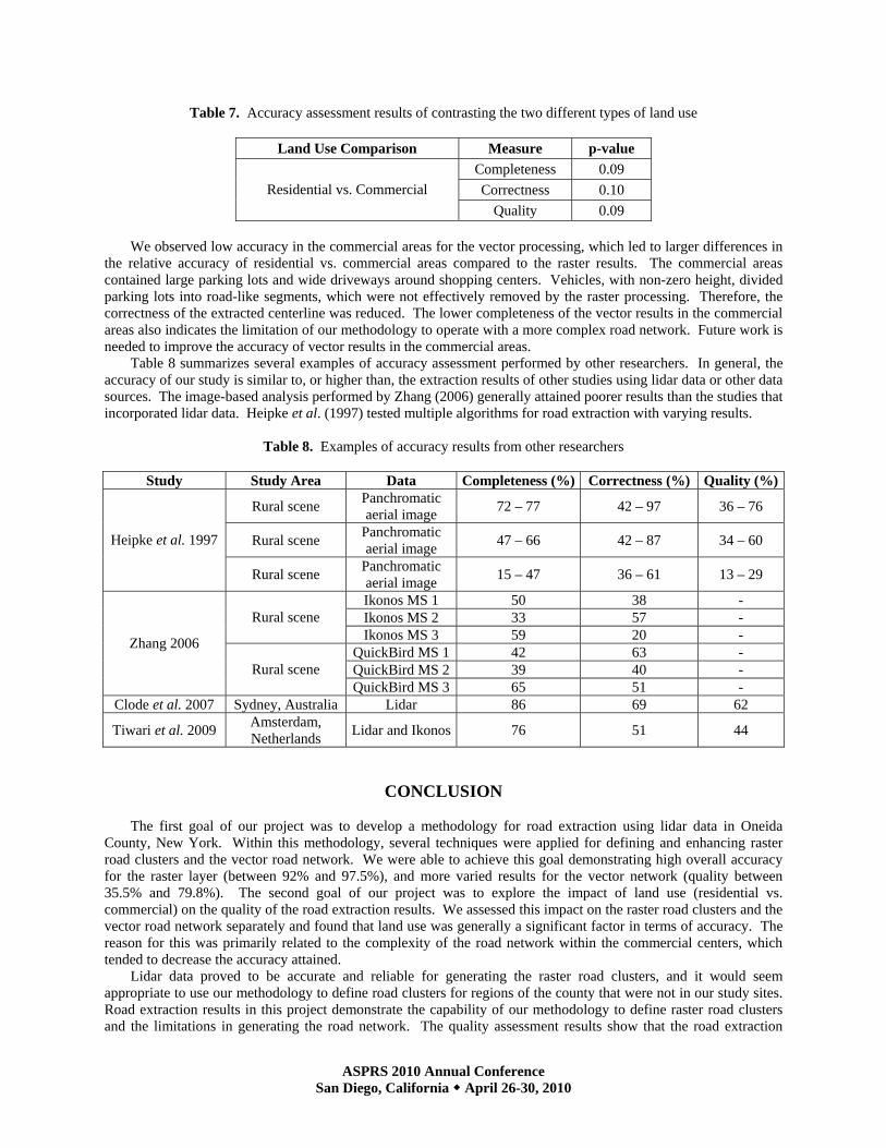
Table 8 summarizes several examples of accuracy assessment performed by other researchers. In general, the accuracy of our study is similar to, or higher than, the extraction results of other studies using lidar data or other data sources. The image-based analysis performed by Zhang (2006) generally attained poorer results than the studies that incorporated lidar data. Heipke et al. (1997) tested multiple algorithms for road extraction with varying results.

Table 8. Examples of accuracy results from other researchers

Study Study Area Data Completeness (%) Correctness (%) Quality (%)

Rural scene Panchromatic aerial image 72 – 77 42 – 97 36 – 76

Rural scene Panchromatic aerial image 47 – 66 42 – 87 34 – 60 Heipke et al. 1997

Rural scene Panchromatic aerial image 15 – 47 36 – 61 13 – 29

Ikonos MS 1 50 38 - Ikonos MS 2 33 57 - Rural scene Ikonos MS 3 59 20 -

QuickBird MS 1 42 63 - QuickBird MS 2 39 40 -

Zhang 2006

Rural scene QuickBird MS 3 65 51 -

Clode et al. 2007 Sydney, Australia Lidar 86 69 62

Tiwari et al. 2009 Amsterdam, Netherlands Lidar and Ikonos 76 51 44

CONCLUSION

The first goal of our project was to develop a methodology for road extraction using lidar data in Oneida County, New York. Within this methodology, several techniques were applied for defining and enhancing raster road clusters and the vector road network. We were able to achieve this goal demonstrating high overall accuracy for the raster layer (between 92% and 97.5%), and more varied results for the vector network (quality between 35.5% and 79.8%). The second goal of our project was to explore the impact of land use (residential vs. commercial) on the quality of the road extraction results. We assessed this impact on the raster road clusters and the vector road network separately and found that land use was generally a significant factor in terms of accuracy. The reason for this was primarily related to the complexity of the road network within the commercial centers, which tended to decrease the accuracy attained.

Lidar data proved to be accurate and reliable for generating the raster road clusters, and it would seem appropriate to use our methodology to define road clusters for regions of the county that were not in our study sites. Road extraction results in this project demonstrate the capability of our methodology to define raster road clusters and the limitations in generating the road network. The quality assessment results show that the road extraction


accuracy was impacted by different types of land use, which suggests future analysis may consider customizing the algorithm parameters depending on the scene characteristics.

REFERENCES Agouris, P., P. Doucette, and A. Stefanidis, 2001. Spatiospectral cluster analysis of elongated regions in aerial

imagery, Proceedings of the IEEE International Conference on Image Processing, 07-10 Oct, Thessaloniki, Greece, pp. 789-792.

Amini, J., M.R. Saradjian, J.A.R. Blais, C. Lucas, and A. Azizi, 2002. Automatic road side extraction from large scale image maps, International Journal of Applied Earth Observation and Geoinformation, 4(2):95-107.

Casella G., and R.L. Berger, 2001. Statistical Inference (Second Edition), Duxbury Press, 688 p. Chanussot, J., G. Mauris, and P. Lambert, 1999. Fuzzy fusion techniques for linear features detection in

multitemporal SAR images, IEEE Transactions on Geoscience and Remote Sensing, 37(3):1292-1305. Clode, S., P. Kootsookos, and F. Rottensteiner, 2004. The automatic extraction of roads from lidar data,

Proceedings of the International Society for Photogrammetry and Remote Sensing, 12-23 July, Istanbul, Turkey, 35:231-236.

Clode, S., F. Rottensteiner, P. Kootsookos, and E. Zelniker, 2007. Detection and vectorization of roads from lidar data, Photogrammetric Engineering and Remote Sensing, 73(5):517-535.

Congalton, R.G., and K. Green, 2009. Assessing the Accuracy of Remotely Sensed Data: Principles and Practices (Second Edition), CRC Press, Taylor & Francis Group, Boca Raton, FL, 183 p.

Duda, R., and K. Hart, 1972. Use of the Hough Transform to detect lines and curves in pictures, Communications of the Association of Computing Machines, 15(1):11-15.

Gibson, L., 2003. Finding road networks in Ikonos satellite imagery, Proceedings of American Society of Photogrammetry and Remote Sensing, Anchorage, Alaska, 5-9, May, CD-ROM.

Haverkamp, D., 2002. Extracting straight road structure in urban environments using Ikonos satellite imagery, Optical Engineering, 41(9):2107-2110.

Heipke, C., H. Mayer, C. Wiedemann, and O. Jamet, 1997. Evaluation of automatic road extraction, in Proceedings of International Archives of Photogrammetry and Remote Sensing, Stuttgart, 17-19 September, Volume 32, Part 3-2W2, pp. 47-56.

Im, J., J.R. Jensen, and J.A. Tullis, 2005. Development of a remote sensing change detection system based on neighborhood correlation image analysis and intelligent knowledge-based systems, IEEE International Geoscience and Remote Sensing Symposium, 25-29 July, Seoul, Korea, Volume 3, pp. 2129- 2132.

Im, J., J. Rhee, J.R. Jensen, and M.E. Hodgson, 2007. An automated binary change detection model using a calibration approach, Remote Sensing of Environment, 106 (1):89-105.

MathWorks, Inc., 2008. Radon Transform, Image Processing Toolbox User's Guide, MATLAB Help Document. Murphy, L.M., 1986. Linear feature detection and enhancement in noisy images via the Radon transform, Pattern

Recognition Letters, 4 (4):279-284. Quackenbush, L.J., 2004. A review of techniques for extracting linear features from imagery, Photogrammetric

Engineering & Remote Sensing, 70(12):1383-1392. Radon, J.H., 1917. Ueber die Bestimmng von Funktionen durch Ihre Integralwerte laengs gewisser

Mannigfaltigkeiten, Reports on the Proceedings of the Saxony Academy of Science, (69):262-277. Song, J.H., S.H. Han, K. Yu, and Y. Kim, 2002. Assessing the possibility of land-cover classification using lidar

intensity data, International Archives of Photogrammetry, Remote Sensing and Spatial Information Sciences Commission III, 9-13 September, Graz, Austria, Volume 34, Part 3B, pp. 259-262.

Toft, P., 1996. The Radon Transform – Theory and Implementation, Ph.D. Thesis, Department of Mathematical Modeling, Technical University of Denmark, Lyngby, Denmark.

Tiwari P.S., H. Pande, and A.K. Pandey, 2009. Automatic urban road extraction using airborne laser scanning/altimetry and high resolution satellite data, Journal of the Indian Society of Remote Sensing, 37(2009): 223–231.

Zhang, Q., 2006. Automated road network extraction from high spatial resolution multi-spectral imagery, Ph.D. Thesis, Department of Geomatics Engineering, University of Calgary, Alberta, CA.

Zhang, Q. and I. Couloigner, 2006a. Benefit of the angular texture signature for the separation of parking lots and roads on high resolution multi-spectral imagery, Pattern Recognition Letters, 27(9):937-946.


Zhang, Q. and I. Couloigner, 2006b. Comparing different localization approaches of the radon transform for road centerline extraction from classified satellite imagery, Proceedings of International Conference on Pattern Recognition, Volume 2, pp. 138-141.

Zhang, Q. and I. Couloigner, 2007. Accurate centerline detection and line width estimation of thick lines using the radon transform, IEEE Transactions on Image Processing, 16(2):310-316.

Zhang, C., S. Murai, and E. Baltsavias, 1999. Road network detection by mathematical morphology, Proceedings of ISPRS Workshop — 3D Geospatial Data Production: Meeting Application Requirements, Paris, pp. 185-200.

road extraction from lidar data in …asprs.org/a/publications/proceedings/sandiego2010/san...asprs...

Documents