hyperspectral biofilm classification analysis for carrying...

Pecora 18 –Forty Years of Earth Observation…Understanding a Changing World November 14 – 17, 2011 ♦ Herndon, Virginia

HYPERSPECTRAL BIOFILM CLASSIFICATION ANALYSIS FOR CARRYING CAPACITY OF MIGRATORY BIRDS IN THE SOUTH BAY SALT PONDS

Wei-Chen Hsu, University of California at Berkeley

Amber Kuss, San Francisco State University Tyler Ketron, Stanford University

Andrew Nguyen, California State University, East Bay Alex Remar, University of Delaware

Michelle Newcomer, San Francisco State University Erich Fleming PhD, SETI Institute, NASA Ames Research Center

Leslie Bebout PhD, NASA Ames Research Center Brad Bebout PhD, NASA Ames Research Center

Angela Detweiler MS, BAER Institute, NASA Ames Research Center J.W. Skiles PhD, NASA Ames Research Center

DEVELOP NASA Ames Research Center M.S. 239-20 Moffett Field, California 94035

[email protected] [email protected]

ABSTRACT

Highly productive tidal marshes provide ecosystem support for migratory birds and often contain biofilm, a substantial food source for the community. In this study, biofilms were analyzed based on taxonomic classification, population density, and spectral signatures. These techniques were then applied to remotely sensed images to map biofilm populations in the South Bay Salt Ponds and predict the carrying capacity of these newly restored ponds for migratory birds. The GER-1500 spectroradiometer was used to obtain in situ spectral signatures for each density-class of biofilm. The spectral variation and taxonomic classification between high, medium, and low density biofilm cover types was mapped using in-situ spectral measurements and classification of EO-1 Hyperion and Landsat TM 5 images. Biofilm samples were also collected in the field to perform laboratory analyses to determine chlorophyll a content, taxonomic classifications, and energy content. Comparison of the spectral signatures between the three density groups shows distinct variations useful for hyperspectral classification. Also, analyses of chlorophyll a concentrations show statistically significant differences between each density group, using the Tukey-Kramer test at an alpha level of 0.05. The potential carrying capacity in South Bay Salt Ponds, an area of approximately 15,000 acres (6,070 hectares), is estimated to be 250,000 birds.

INTRODUCTION

Development of over 90% of the South San Francisco Bay estuary in the past century, from a natural wetland environment to agricultural and salt production ponds, has lowered biodiversity while weakening the ability for this ecosystem to aid in flood protection and pollution control (Philip Williams & Associates Ltd. and Faber, 2004). In an effort to restore 15,000 acres of this land, the South Bay Salt Pond Restoration Project (SBSPRP) has applied an adaptive management strategy for wetland restoration (Trulio et al., 2007). The SBSPRP is managed collaboratively by the California State Coastal Conservancy (CSCC), the U.S. Fish and Wildlife Service (FWS), and the California Department of Fish and Game (DFG) (Trulio et al., 2007; South Bay Salt Pond Restoration, 2010).

Tidal marshes are highly productive ecosystems, providing habitat for birds, breeding grounds for fish and crabs, flood protection, and improved water quality through pollutant filtration (Kelly and Tuxen, 2009). The South Bay salt ponds, located at the southern end of San Francisco Bay, lie on the Pacific Flyway, which provides good roosting and over-wintering sites for migratory bird species and also a rich supply of nutrients on the mudflats. The shallow open water, mudflats, and salt marshes are utilized by various waterfowl, shorebirds, and mammals (Siegel and Bachand, 2002). It was estimated that over 500,000 birds utilize the habitat each year in the San Francisco Bay Salt Ponds (Harrington and Perry, 1995). Many small shorebirds use seasonal managed ponds throughout the year, with highest usage during spring, fall, and winter period (Brand et al., 2011).


Within newly restored mudflats and wetlands, microbial processes play a critical role in sediment stability, re-mineralization of nutrients, and primary and secondary productivity (Decho, 1990; Kuwae et al., 2008; Murphey et al., 2008a). The presence of microphytobenthos, commonly referred to as biofilms, on the surface of tidal mudflats indicates the ability for the newly restored pond to support flora and fauna (Characklis and Marshall, 1990). Biofilms have a green to brownish green color, and consist of a thin, (0.01−2mm) dense layer of microbes, including diatoms and algae, and sediment held together by an extracellular polymeric matrix (EPS) that creates a stable living environment for microbes (Characklis and Marshall, 1990; MacIntyre et al., 1996; Decho, 1990; Paterson et al., 1998; Decho, 2000). Biofilm have a highly variable density distribution, with low to high density areas located in close proximity. (MacIntyre et al., 1996; Murphy et al., 2008a). Tidal cycle, nutrient and light availability, and desiccation contribute to the heterogeneity of biofilms (Underwood and Kromkamp, 1999; Cartaxana et al., 2006). Additionally, the surface density is tidal cycle and sunlight dependent as biofilms members migrate vertically through the sediment column (MacIntyre et al., 1996; Murphy et al., 2008a).

Intertidal biofilms are critical to the health of the wetland ecosystem, and contribute substantially to the food web by supporting a variety of species including mollusks, crustaceans, insects, and shorebirds (MacIntyre et al., 1996; Barillé et al., 2007; Kuwae et al., 2008). Biofilms are one of the primary food source for macroinvertebrates, but a recent study by Kuwae et al. (2008), found that biofilms also contribute to a significant portion (45-59%) of the food diet for the Western Sandpiper (Calidris mauri) in Canada. More than 69 species of shorebirds use the South San Francisco Bay for overwintering and migration indicating the presence of a previously unrecognized food source for these birds in the San Francisco Bay (Takekawa et al., 2006)

Previous studies have indicated that biofilms could be accurately mapped using remotely sensed data (Méléder et al., 2003; Combe et al., 2005; Cartaxana et al., 2006; Jesus et al., 2006; Murphy et al., 2008a; Murphy et al., 2008b). The advantages of using remote sensing to conventional sampling approaches includes the ability to perform non-destructive analysis in ecologically sensitive and difficult to access areas, and the large spatial coverage provided by airborne/satellite sensors (Adam et al., 2010; Jonson et al., 1980; Murphy et al., 2008b). Mapping the biofilm presence in newly restored wetland habitats can provide useful information required for the continued management of the South Bay estuary. In addition to their benefit as a food source, EPS created by the microphytobenthos holds sediment grains together and increases sediment stability, which is important to promote colonization of primary wetland vegetation (Takekawa et al., 2006; Adam et al., 2010). Thus, the presence of biofilm could be a useful indicator for management agencies to assess the health and overall progress of newly restored ponds.

In this study, remotely sensed as well as in-situ data were used to assess the capacity of newly restored wetlands to support a diverse community in the South San Francisco Bay. The goals of this project were to: 1) provide a taxonomic classification of the dominant biofilm species within the ponds and the intertidal mudflats, 2) to monitor the spatial distribution and density of biofilms throughout the South Bay, and 3) to estimate the number of shorebirds that can be supported in this ecosystem based on biofilm biomass and energy content. The first goal will provide a basis for understanding the variation of diatoms and other algae throughout the ponds as well as provide insight into the primary environmental factors contributing to the growth of a particular species. The spatial distribution of biofilms was analyzed using multiple sensors including EO-1 Hyperion, Landsat-5 Thematic Mapper, IKONOS, and the Advanced Spaceborne Thermal Emission and Reflection Radiometer (ASTER). Spectral signatures from the different biofilm categories were statistically correlated with in-situ measurements collected during Fall 2010 and Spring 2011 using a handheld GER 1500 spectrophotometer. In-situ spectra were compared with image spectra using various hyperspectral classification algorithms including the Spectral Angle Mapper (SAM), supervised classification, and derivative analysis. An identification of multiple biofilm categories allowed for accurate mapping of biofilm distribution and density throughout the South Bay. Chlorophyll a (Chl a) content, measured in µg/cm2 of sediment, was used to differentiate the biofilm density categories. Finally, the carrying capacity of the South Bay was estimated using an equation that incorporates the area covered by biofilm, the biofilm biomass, the biofilm energy density, and the shorebird consumption rate. Study Area

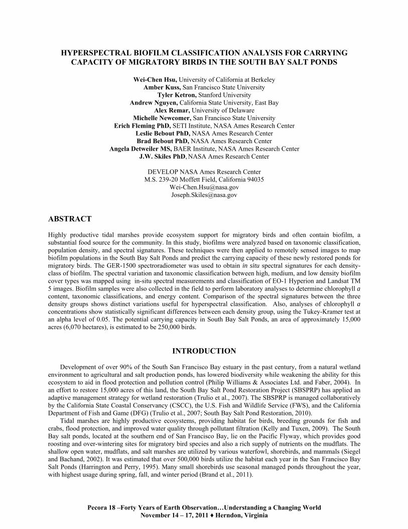
The SBSPRP is underway at the southern end of the San Francisco Bay at three primary restoration sites: Ravenswood, Eden Landing and Alviso (Figure 1). Ground truth measurements and spectroradiometer readings for this project were performed in each of these sites.


METHODOLOGY Field Methods

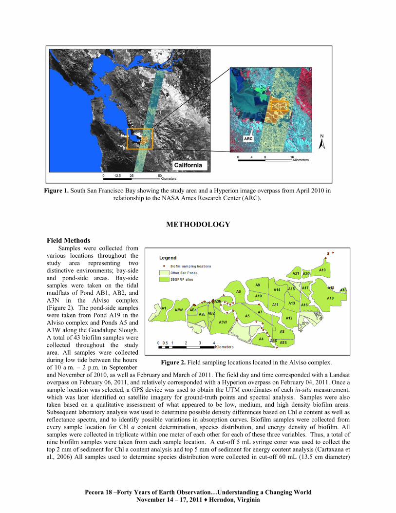
Samples were collected from various locations throughout the study area representing two distinctive environments; bay-side and pond-side areas. Bay-side samples were taken on the tidal mudflats of Pond AB1, AB2, and A3N in the Alviso complex (Figure 2). The pond-side samples were taken from Pond A19 in the Alviso complex and Ponds A5 and A3W along the Guadalupe Slough. A total of 43 biofilm samples were collected throughout the study area. All samples were collected during low tide between the hours of 10 a.m. – 2 p.m. in September and November of 2010, as well as February and March of 2011. The field day and time corresponded with a Landsat overpass on February 06, 2011, and relatively corresponded with a Hyperion overpass on February 04, 2011. Once a sample location was selected, a GPS device was used to obtain the UTM coordinates of each in-situ measurement, which was later identified on satellite imagery for ground-truth points and spectral analysis. Samples were also taken based on a qualitative assessment of what appeared to be low, medium, and high density biofilm areas. Subsequent laboratory analysis was used to determine possible density differences based on Chl a content as well as reflectance spectra, and to identify possible variations in absorption curves. Biofilm samples were collected from every sample location for Chl a content determination, species distribution, and energy density of biofilm. All samples were collected in triplicate within one meter of each other for each of these three variables. Thus, a total of nine biofilm samples were taken from each sample location. A cut-off 5 mL syringe corer was used to collect the top 2 mm of sediment for Chl a content analysis and top 5 mm of sediment for energy content analysis (Cartaxana et al., 2006) All samples used to determine species distribution were collected in cut-off 60 mL (13.5 cm diameter)

Figure 1. South San Francisco Bay showing the study area and a Hyperion image overpass from April 2010 in relationship to the NASA Ames Research Center (ARC).

Figure 2. Field sampling locations located in the Alviso complex.


syringe cores. The biofilm density, the location of the biofilm, and the Chl a content, along with values provided by Kuwae et al. (2008), are inputs into carrying capacity calculations.

Satellite Remote Sensing

All satellite imagery was geometrically and radiometrically corrected to reflectance and re-projected to the UTM WGS 84 North projection to ensure tonal and spatial comparability between each scene using Earth Resources Data Analysis System (ERDAS) IMAGINE software (Earth Resources Data Analysis System, 2010). Multiple airborne and satellite sensors were used to compare spectra of satellite sensors with in- situ GER measurements. Three sensors were used, the EO-1 Hyperion satellite sensor, the IKONOS satellite, and the Landsat-5 Thematic Mapper (Table 1). The Hyperion sensor is multispectral and obtains 220 bands at 10 nm bandwidth with a swath of 7.5 km and a resolution of 30 m. The IKONOS satellite is a high resolution satellite with approximately 1 m resolution, and provides four bands for analysis. The Landsat-5 satellite has the same resolution as Hyperion (30 m) but contains only bands 1−7. Atmospheric and radiometric corrections were performed using the empirical line calibration method.

Landsat TM5. Imagery from the Landsat-5 TM sensor was used for analyzing the general distribution of

biofilm and vegetation throughout the salt ponds. The Normalized Differenced Vegetation Index (NDVI) was used to calibrate the images to a relative vegetation index, and then thresholds were applied using areas of known vegetation and biofilm location. The NDVI images were acquired from 2006-2011 to monitor general vegetation trends and to assess the accuracy of the biofilm classification. After threshold values for biofilm were applied to the NDVI images, all the images were combined to create a map that shows probable biofilm distribution.

IKONOS. IKONOS images were obtained in June 2008, and July 2010 from our partners of the SBSPRP. These images were also calibrated to NDVI for accuracy assessment purposes. The IKONOS images were not used for calculating areas of biofilm distribution, but rather were used for qualitative purposes such as accuracy assessment and initial field site selection.

Hyperion. Images from the Hyperion instrument were obtained in March and July of 2010 and February 2011. The EO-1 Hyperion is a hyperspectral satellite sensor that collects a total of 220 spectral channels with a 10-11nm bandwidth at a 30 m resolution for every channel (Simon and Beckmann, 2005). Hyperion scenes do not have a predictable temporal resolution because they can only be acquired upon specific request by the general public. Hyperion imagery was atmospherically corrected and converted from radiance to surface reflectance values using Environment for Visualizing Images (ENVI) image processing software program (ITT Visual Information Solution, 2011) and the plug-in module, FLAASH (Research Systems Inc., 2005). Hyperion Imagery was spectrally subset to only evaluate between 426.82 nm to 905.05 nm, which is the most indicative window for detecting biofilm based on the derivative analysis (see below). Accordingly, only 48 of the total 220 Hyperion bands were used in the analysis. All Hyperion imagery was then georectified using a total of 20 ground control points (GCP) and two georeferenced vector files: one shapefile outlining the Alviso salt ponds and one vector file containing California highways. Such image processing is necessary to ensure accurate tonal and spatial comparability between each Hyperion scene. Orthorectification of the Hyperion image was omitted because the terrain in the study area was relatively flat and close to sea level.

Using the spectral analysis workstation in ERDAS IMAGINE, a total of 2 spectral libraries were constructed and then implemented as the reference or target spectra to classify each Hyperion image. The first library used the GER 1500 data (averaged and then converted to apparent reflectance), and the second library used image-derived spectral data based on the known densities and locations of biofilm mapped during fieldwork using GPS coordinates. The cosine function of the spectral angle mapper (SAM) classification algorithm was then applied to the Hyperion image (Equation 1).

Sensor Purpose Bands Used

Wavelengths (µm) Resolution (m) Dates used Image Source

Landsat 5 TM

Detect Vegetation

3 0.45-0.69 30 8/18/94, 8/22/07,

8/27/09, 7/5/10, 2/6/11 Glovis

(USGS, 2010a)

IKONOS Detect

Vegetation Visible region 1 2008,2009, 2010 GeoEye

Hyperion on EO-1

Obtain spectral curve for biofilm

48 0.426- 0.905

30 7/7/10, 2/4/11 Glovis

(USGS, 2010a)

Table 1: Satellite sensors used in the biofilm mapping analysis.


Equation (1)

n

ii

n

ii

n

iii

yx

yx

22

1cos

where: n = number of bands α = angle formed between reference spectrum and image spectrum x = image spectrum y = reference or target spectrum

The cosine SAM algorithm computes a spectral angle between a target spectrum and each pixel in the image using all of the bands in the image (Shippert, 2003). The lower the spectral angle value between a pixel and a target spectrum, the more similar the pixel and target. The image spectrum (variable x in equation 1), corresponds to all pixels within each image that are to be analyzed. The reference or target spectra were obtained from the two aforementioned spectral libraries. Low and high density biofilms were used as the input target spectra for both classifications. Laboratory Analysis

All of the field samples were processed at NASA Ames and the UC Davis Ecology Laboratory. Table 2 shows the laboratory procedure used for each variable of interest.

Energy Content. A bomb calorimeter was used to measure the energy capacity of each biofilm sample as higher

heat in MJ/kg. Samples were divided into three density categories using qualitative visual observation, low (7 samples), medium (5 samples), and high (5 samples). Each category consists of one to eight samples within each GPS sampling point, totaling to 17 samples collected per day. After sample collection, the top 2 mm of 5 mL syringe cores were weighed and the net weight was recorded. The 17 samples were freeze dried for approximately 72 hours to remove moisture from the sample. We chose freeze dry as a viable method as opposed to drying in low temperature (45-50C) to reduce the possibility of caramelizing the sample, that would have further cause the sample to lose organic compounds through the heating process (Wei Yu, UC Davis personal communication, 2011). After the samples were dried and weighted to obtain the final mass, the samples were crushed with a pestle and mortar and mixed with benzoic acid to encourage combustion. A pellet press was used to form a mixture of biofilm/benzoic acid to further ensure complete combustion. The total higher heat value of the biofilm/benzoic acid mixture was applied to the following equation in order to calculate biofilm higher heat value:

Equation (2) where: HHV= higher heat value b= biofilm ben= benzoic acid tot= total M= mass

Chlorophyll a using Biomass Spectroscopy. To evaluate the density of the biofilm spectroscopy reference measurements were performed using a methanol extraction technique to determine Chl a content of a biofilm sample

Variable Field Collection Method Laboratory Processing Technique

Energy content (J/g) First 2mm biofilm sediment core Calorimeter

Chlorophylla (µg/cm2) First 2mm of biofilm sediment core UV spectrophotometer 1800

Taxonomy First 5mm of biofilm sediment core Axium microscope

Spectral curve GER 1500 Spectrophotometer Output curves plotted in remote sensing software

b

benbentottotb M

MHHVMHHVHHV

Table 2: Laboratory analysis used for each variable of interest.


(Tett et al., 1975). Methanol was applied to each of the triplicate samples and allowed to soak overnight to extract methanol soluble pigments including Chl a. Samples were centrifuged to remove particulates and the absorbance of the supernatant at 665 nm was measured in a Shimadzu UV1800 spectrophotometer. The absorbance at 750 nm was subtracted to remove background absorbance. Pheophytin absorbance, which overlaps with Chl a at 665 nm, was corrected for using the acidification method. Hydrochloric acid was added to each sample to 1M to convert all Chl a to pheophytin. The acidified samples were then measured at Abs665 and Abs750.The equation below was used to separate pheophytin from Chl a absorbance. Equation (3) where: C= concentration of Chl a in the sample O = Abs665 of methanol extract A= Abs665 of acidified methanol extract Ec= extinction coefficient of chlorophyll a at 665 nm in methanol Ep= extinction coefficient of pheophytin a at 665 nm in methanol

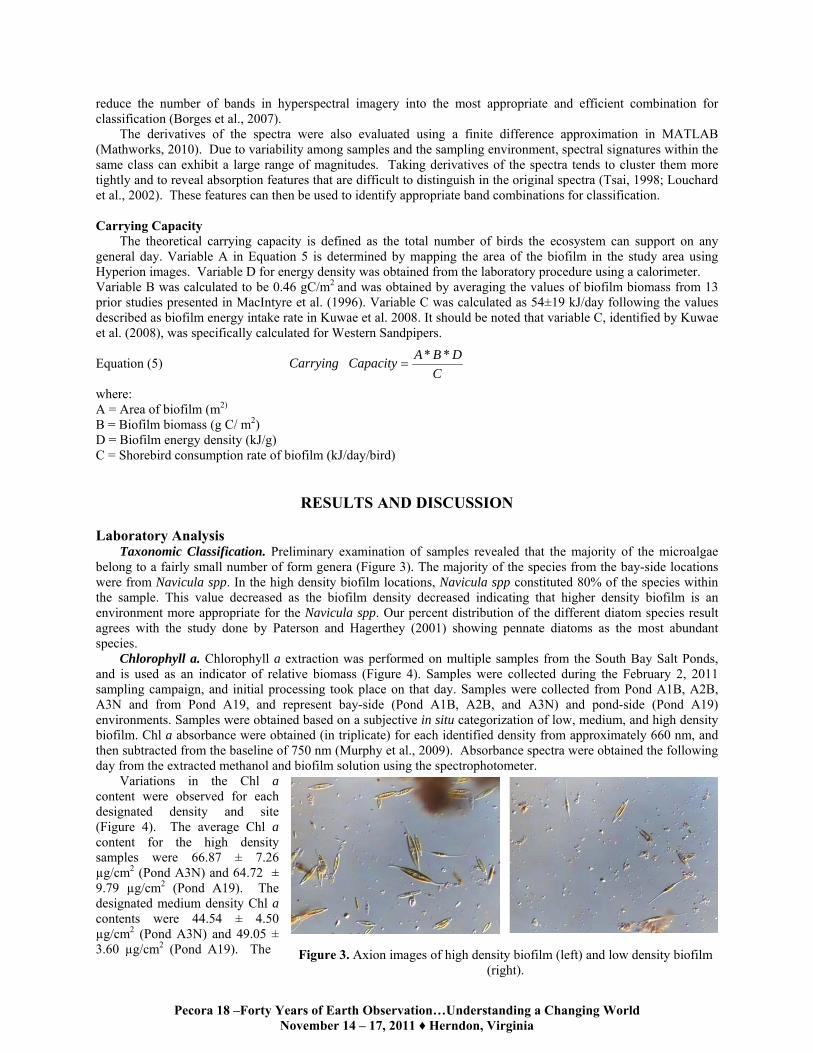
Taxonomic Classification. An estimation of the microbial population at each site was obtained from the triplicate 60 mL core samples to identify the dominant taxa in both the bay-side and pond-side locations. Microscope snapshots were taken of the bay-side and pond-side samples (Figure 3). To identify the population distribution of different species of diatoms, a standardized counting method was used. For each sample, 40 snapshots were taken and each different species was counted, and the relative percent abundance of each species was calculated For each sample, several slides were screened under a Nikon Microphot�FXA microscope (Figure 3). The slides are representative of the natural samples and were not cleaned or cultivated in order to observe characteristic community distributions. Relative numbers of the most common microorganisms present in each sample were obtained by counting cells in random fields of view on a glass slide (Ribeiro et al., 2003). Individual cells were examined under high magnification and multiple sample images were obtained for each triplicate to determine the dominant diatom genera. An appropriate (and exactly the same) number of cells were counted for each slide analyzed. GER-1500 Spectroradiometer-Field Spectrometry

Spectra were recorded using the handheld GER 1500 spectroradiometer (Spectra Vista Corporation, 2010) at each location before core samples were taken. When sampling, locations were visually classified into one of four categories: high, medium, or low density biofilm, or mud. At each sample location three replicate spectra were taken and later averaged to produce a single representative spectrum. Areas covered by water were avoided. Prior to each spectral measurement, three calibration spectra were recorded from a ~99% reflective panel. Spectra were taken at a 5–6 ft height above the mudflat to accommodate a field of view of 10-12 cm. Then the GER spectra were converted from digital number to reflectance, and resampled to only contain 400–900 nm wavelength. The GER data were then analyzed using both traditional statistical techniques and a qualitative derivative analysis.

The mean and standard deviation of each group of spectra were calculated to obtain a single representative spectrum for each class of low, medium, and high density biofilm. The spectral classification groups were also tested for distinctness by using the Jeffries-Matusita (JM) distance, shown in Equation 4 (Tsai, 2002). Equation (4) where: i and j = two class signatures being compared µ = mean across all class samples ∑ = class covariance matrix

The JM distance has a maximum value of 1.41, which indicates that the two classes are entirely separable, and a minimum value of 0, which indicates that the two classes are not separable at all. The JM distance can be used to

ji

jiji

jiTji

ij eJM

2/ln

2

1

28

1

12

1

cb EE

AOC


reduce the number of bands in hyperspectral imagery into the most appropriate and efficient combination for classification (Borges et al., 2007).

The derivatives of the spectra were also evaluated using a finite difference approximation in MATLAB (Mathworks, 2010). Due to variability among samples and the sampling environment, spectral signatures within the same class can exhibit a large range of magnitudes. Taking derivatives of the spectra tends to cluster them more tightly and to reveal absorption features that are difficult to distinguish in the original spectra (Tsai, 1998; Louchard et al., 2002). These features can then be used to identify appropriate band combinations for classification. Carrying Capacity

The theoretical carrying capacity is defined as the total number of birds the ecosystem can support on any general day. Variable A in Equation 5 is determined by mapping the area of the biofilm in the study area using Hyperion images. Variable D for energy density was obtained from the laboratory procedure using a calorimeter. Variable B was calculated to be 0.46 gC/m2 and was obtained by averaging the values of biofilm biomass from 13 prior studies presented in MacIntyre et al. (1996). Variable C was calculated as 54±19 kJ/day following the values described as biofilm energy intake rate in Kuwae et al. 2008. It should be noted that variable C, identified by Kuwae et al. (2008), was specifically calculated for Western Sandpipers. Equation (5)

where: A = Area of biofilm (m2) B = Biofilm biomass (g C/ m2) D = Biofilm energy density (kJ/g) C = Shorebird consumption rate of biofilm (kJ/day/bird)

RESULTS AND DISCUSSION Laboratory Analysis

Taxonomic Classification. Preliminary examination of samples revealed that the majority of the microalgae belong to a fairly small number of form genera (Figure 3). The majority of the species from the bay-side locations were from Navicula spp. In the high density biofilm locations, Navicula spp constituted 80% of the species within the sample. This value decreased as the biofilm density decreased indicating that higher density biofilm is an environment more appropriate for the Navicula spp. Our percent distribution of the different diatom species result agrees with the study done by Paterson and Hagerthey (2001) showing pennate diatoms as the most abundant species.

Chlorophyll a. Chlorophyll a extraction was performed on multiple samples from the South Bay Salt Ponds, and is used as an indicator of relative biomass (Figure 4). Samples were collected during the February 2, 2011 sampling campaign, and initial processing took place on that day. Samples were collected from Pond A1B, A2B, A3N and from Pond A19, and represent bay-side (Pond A1B, A2B, and A3N) and pond-side (Pond A19) environments. Samples were obtained based on a subjective in situ categorization of low, medium, and high density biofilm. Chl a absorbance were obtained (in triplicate) for each identified density from approximately 660 nm, and then subtracted from the baseline of 750 nm (Murphy et al., 2009). Absorbance spectra were obtained the following day from the extracted methanol and biofilm solution using the spectrophotometer.

Variations in the Chl a content were observed for each designated density and site (Figure 4). The average Chl a content for the high density samples were 66.87 ± 7.26 µg/cm2 (Pond A3N) and 64.72 ± 9.79 µg/cm2 (Pond A19). The designated medium density Chl a contents were 44.54 ± 4.50 µg/cm2 (Pond A3N) and 49.05 ± 3.60 µg/cm2 (Pond A19). The Figure 3. Axion images of high density biofilm (left) and low density biofilm

(right).

C

DBACapacityCarrying

**


low density Chl a contents are 21.76 ± 2.22 and 25.18 ± 1.73 µg/cm2 (Ponds A3N and A19, respectively). Each subjectively identified field category (low, medium, and high), was identified as statistically different according to the Tukey-Kramer test at the alpha level of 0.05 (Tukey, 1977; JMP Version 7, 2007). These findings support the conclusion that wetland systems are highly variable, and that varying densities in close proximity (within 1−3 m) can have multiple Chl a contents and therefore biomass differences. Additionally, due to the extraction method, the Chl a values will be slightly lower than in situ values.

Caloric Analysis. Dividing the samples into their respective density categories and sorting the sample data from lowest to highest energy value revealed an increasing caloric trend from low to medium. However, there is an overlap between the highest medium (6.365 MJ/kg) and lowest high (1.949 MJ/kg) density samples. Based on the caloric analysis, the medium and high density categories are not statistically different; although this is not consistent with the Chl a analysis and our field observations. As mentioned in the field methodology section, the definition of density classes were based on qualitative field observations and are considered arbitrary. Linking these data to our chlorophyll measurements has supported a possibility of two density levels instead of our perceived three. Final results for caloric value calculated as averages per density category are 2.554 MJ/kg (low), 4.727 MJ/kg (medium), and 4.303 MJ/kg (high).

Figure 3. Percent distribution of the different species found in one of the bay-side sampling location.

0.00%

10.00%

20.00%

30.00%

40.00%

50.00%

60.00%

70.00%

80.00%

90.00%

Navicula spp. Gyrosigma fasciola-type

Gyrosigma acuminatum-like

Cylindrotheca closterium-like

Cylindrotheca fusisormis

Gyrosigma spp.

Percent Distribution of Different Taxonomic Species

Low Density

Medium Density

High Density

Figure 4. Chlorophyll a content in Ponds A3N (site 32) and A19

(site 34). Samples are categorized based on low (L),

medium (M), and high (H) observational densities.


Figure 6. Biofilm density distribution using SAM classification of Hyperion images.

Landsat Biofilm Probability Distribution Map NDVI of multiple Landsat images was combined to

construct a biofilm probability map that shows how consistent biofilm exists in a location (Figure 5). Pixels where biofilms were classified more often appears closer to red, while pixels where biofilms were classified less often appear yellow. This method thus produced a map which shows the probability of biofilm presence.

Hyperion Classification: Spectral Angle Mapper (SAM) Biofilm distribution in the South San Francisco Bay was mapped using the SAM classification of Hyperion

images (Figure 6). Spectra of observed low, medium, and high biofilm densities were applied to the Hyperion images from July, 2010 and February, 2011. Prior to application of the SAM classification, in situ GER measurements taken from each sampling campaign were combined based on class and averaged to provide three representative spectra. The SAM calculated the spectral similarity between a test reflectance spectrum (each different biofilm class) and the spectrum for each pixel in the Hyperion images (Li et al., 2008). The cross-correlation coefficient identified the presence of biofilm-like spectra for each pixel in the image. Biofilm-like pixels in the image were classified with correlations of > 0.990, identifying pixels that are similar to the 99th percentile. These images were then subset and imported into ArcGIS for identification of percent area coverage of each biofilm category.

Biofilm locations in the study area were accurately mapped for two distinct densities. Although from previous analysis (including Chl a), there are three (low, medium and high) significantly different classes of biofilm densities, there are spectral similarities in the low and medium classes, using derivative analysis. Therefore, in the image processing, these two categories were identified in similar locations within the study area. Due to these spectral similarities, subsequent classification maps were generated based on two biofilm density classes, low and high. A map combining the low and medium categories with a distinct high category provides the most accurate biofilm map (Figure 6). In the classified map, two unique areas of interest were observed as suitable habitat for biofilm development, along tidal sloughs and on tidal mudflats within the ponds and in the bay. These maps were also used to

calculate the total area of biofilm with the South Bay Salt Ponds. Although there are two distinctly mapped classes, the total

area for both classes was used to make an estimate of carrying capacity in the study area. The total area calculated from the classification maps is 28.6 million m2. This was the value used for A in Equation 5.

Figure 5: Probability map depicting likelihood of biofilm. presence.


GER Spectra Analysis The JM distances revealed that the most relevant band ranges for classification were 425–550 nm and 590–690

nm. While most band combinations showed a high degree of separability within this range, the JM distances between the low density and medium density biofilms were much lower than the other class combinations, indicating that the low and medium density were more similar and perhaps should not be identified as separate classes. Similarly, the derivative analysis also showed that the low and medium density classes were more similar than other classes. However, the derivative spectra revealed additional absorption features that can be used in the future to improve classification accuracy. The analysis also revealed additional features to help classification between high density biofilms and vegetation. Spectral analysis shows that biofilm spectra are similar to vegetation which can be observed from the classification where it’s difficult to distinguish biofilm from vegetation for some of the areas. Carrying Capacity Assessment

The shorebird carrying capacity of the South Bay salt pond restoration area was estimated using four variables outlined in Equation 5. Using the Hyperion classification-SAM method, the area of biofilm was mapped and calculated to be 28,641,600 m2. Values for biofilm energy density and shorebird consumption rate of biofilm were obtained by results presented in Kuwae et al. (2008), and were found to be 0.83 KJ/g for variable D, and 54±19 kJ/day for variable C. The low and high error values for biofilm energy density were used to determine the range of the study area’s carrying capacity. After using the aforementioned values in Equation 5, the shorebird carrying capacity of the South San Francisco Bay salt pond restoration area was calculated to be approximately 201,000 shorebirds per day. Considering the South Bay Salt Ponds are still in the initial stages of restoration, the value obtained from this study was reasonable, and it is expected that the number of shorebirds supported will grow as more ponds are restored.

CONCLUSION

The carrying capacity for the South Bay Salt Ponds was calculated in this study to estimate the growing population of shorebirds this wetland can support. A remote sensing approach using the NASA EO-1 Hyperion sensor was used to map and quantify the distribution of biofilm throughout the South San Francisco Bay. Using field locations and spectral readings of low, medium, and high density biofilm locations, similar categories (low and high) were mapped in the Hyperion images during a low-tide overpass. Field samples were taken at the same time as the spectral measurement to determine taxonomy, chlorophyll a content, and energy content. These values coupled with the quantified area the biofilm covers, were used to calculate the carrying capacity of the south bay in terms of the number of birds supported per day. Biofilm contributes a significant portion of calories to a bird’s diet (Kuwae et al., 2008) and this analysis calculated that current distribution of biofilm can support approximately 201,000 birds per day. This value is a preliminary estimate based on mapped areas of biofilm only for the south bay and it is assumed that this value would increase if Eden Landing and Ravenswood ponds were also included in the calculations.

In this study, the spatial distribution of the biofilm was successfully mapped using various satellite sensors and techniques. However, the limitation with the use of remote sensing imagery is that the classification is only able to capture the spatial distribution of biofilm during a short period of time that it only capture the relative density and biomass of biofilm and does not necessary reflect the actual density of biofilm at all times due to highly variable (related to density, spatial proximity, and seasonal changes) characteristics of biofilms.

ACKNOWLEDGEMENTS

We thank Dr. Randy Berthold, John Preston, and Matt Linton for making the NASA DART boats available for our sampling campaign. We also thank Lee Johnson for making the GER 1500 available to us, and for accompanying us on our fieldwork. We also thank Dr. John Takekawa, Dr. Tomohiro Kuwae, and Monica Iglecia for accompanying us for fieldwork and scientific support. We also thank UC Davis Lab (Bryan Jenkins, and Chao) for making their calorimeter facilities available to us and providing laboratory assistance. We also thank Brian Fulfrost, Cheryl Strong, Brad Lobitz, and Dr. Liana Guild for their help and support with this project.


REFERENCES Adam, S., A. D. Backer, A. D. Wever, K. Sabbe, E. A. Toorman, M. Vincx, and J. Monbaliu. 2010. Bio-physical

characterization of sediment stability in mudflats using remote sensing: a laboratory experiment. Continental Shelf Research. In press.

Barillé, L., V. Méléder, J. P. Combe, P. Launeau, Y. Rincé, V. Carrčre, and M. Morançais, 2007. Comparative analysis of field and laboratory spectral reflectances of benthic diatoms with a modified Gaussian model approach, Journal of Experimental Marine Biology and Ecology, 343(2): 197–209.

Brand L. A., J. Takekawa, I. Woo, J. Bluso-Demers, J. Shinn, T. Graham, E. Mruz, J. Krause, and C. Strong. 2011. Shorebird and duck responses to pond management in the South Bay Salt Ponds. Retrieved from: http://www.southbayrestoration.org/science/2011symposium/presentationposter/2011_Brand_SBSPRPSymposium.pptx.pdf.

Borges, J. S., A. R. Marçal, and J. M. Dias, 2007. Evaluation of feature extraction and reduction methods for hyperspectral images, in Proceedings of the 26th EARSeL Symposium-New Developments and Challenges in Remote Sensing, 255–264.

Cartaxana, P., C. R. Mendes, M. A. van Leeuwe, and V. Brotas, 2006. Comparative study on microphytobenthic pigments of muddy and sandy intertidal sediments of the Tagus estuary, Estuarine, Coastal and Shelf Science, 66(1-2): 225–230.

Characklis, W. G., and K. C. Marshall, 1990. Biofilms, John Wiley and Sons. pp., 816. Combe, J., P. Launeau, V. Carrére, D. Despan, V. Méléder, L. Barillé, and C. Sotin. 2005. Mapping

microphytobenthos biomass by non-linear inversion of visible-infrared hyperspectral images. Remote Sensing of Environment, 98: 371–387.

Decho, A.W., 1990. Microbial exopolymer secretions in ocean environments: their role(s) in food webs and marine processes. Oceanography and Marine Biology: an Annual Review, 28: 73–153.

Decho, A., 2000. Microbial biofilms in intertidal systems: an overview, Continental Shelf Research, 20: 1257–1273. Earth Resources Data Analysis System, ERDAS, 2010. http://www.erdas.com/Homepage.aspx Harrington, B. and E. Perry. 1995. Important shorebird staging sites meeting western hemisphere shorebird reserve

network criteria in the United States. United States Department of the Interior, Fish and Wildlife Service. ITT Visual Information Solution, Environment for Visualizing Images (ENVI), 2010. http://www.ittvis.com/ Jesus, B., C. R. Mendes, V. Brotas, and D. M. Paterson, 2006. Effect of sediment type on microphytobenthos

vertical distribution: Modelling the productive biomass and improving ground truth measurements, Journal of experimental marine biology and ecology, 332(1): 60–74.

Jonson, D., R. Zingmark, and S. Katzberg, 1980. Remote Sensing of Benthic Microalgal biomass with a tower-mounted multispectral scanner, Remote Sensing of Environment, 9: 351–362.

JMP, Version 7. 2007. SAS Institute Inc., Cary, North Carolina. Kelly, M. and Tuxen, K, 2009. Remote Sensing and Geospatial Technologies for Costal Ecosystem Assessment and

Management. Springer-Verlag Berlin Heidelberg pp. 341-363. Kuwae, T., P. G. Beninger, P. Decottignies, K. J. Mathot, D. R. Lund, and R. W. Elner, 2008, Biofilm grazing in a

higher vertebrate: the Western Sandpiper, Calidris mauri, Ecology, 89(3): 599–606. Li, Z., J. Chen, and E. Baltsavias, 2008. Advances in photogrammetry, remote sensing and spatial information

sciences: 2008 ISPRS congress book, CRC Press/Balkema, Great Britian. Louchard, E. M., R. P. Reid, F. C. Stephens, C. O. Davis, R. A. Leathers, T. V. Downes, and R. Mafflone, 2002.

Derivative analysis of absorption featurerrs in hyperspectral remote sensing data of carbonate sediments, Optics Express, 10(28): 1574–1584.

MacIntyre, H. L., R. J. Geider, and D. C. Miller. 1996. Microphytobenthos: the ecological role of the “Secret Garden” of unvegetated, shallow-water marine habitats. I. Distribution, abundance and primary production. Estuaries, 19 (2A): 186–201.

Mathworks , MATLAB, R2010a. http://www.mathworks.com/ Méléder, V., L. Barillé, P. Launeau, V. Carrère, and Y. Rincé, 2003. Spectrometric constraint in analysis of benthic

diatom biomass using monospecific cultures, Remote Sensing of Environment, 88(4): 386–400. Murphy, R. T., T. J. Tolhurst, M. G. Chapman, and A. J. Underwood. 2008a. Spatial variation of chlorophyll on

estuarine mudflats determined by field-based remote sensing. Marine Ecology Progress Series, 365:45–55. Murphy, R. J., A. J. Underwood, T. J. Tolhurst, and M. G. Chapman, 2008b, Field-based remote-sensing for

experimental intertidal ecology: Case studies using hyperspatial and hyperspectral data for New South Wales (Australia), Remote Sensing of Environment, 112(8): 3353–3365.


Murphy, R. J., A. J. Underwood, and A. C. Jackson, 2009. Field-based remote sensing of intertidal epilithic chlorophyll: Techniques using specialized and conventional digital cameras, Journal of Experimental Marine Biology and Ecology, 380(1-2): 68–76.

Paterson, D. M., K. H. Wiltshire, A. Miles, J. Blackburn, I. Davidson, M. G. Yates, S. McGrorty, and J. A. Eastwood, 1998. Microbiological Mediation of Spectral Reflectance from Intertidal Cohesive Sediments, Limnology and Oceanography, 43(6): 1207–1221.

Paterson, D. M., and S. E., Hagerthey. 2001. Microphytobenthos in contrasting coastal ecosystems: Biology and dynamics. In K. Reise (Ed), Ecological comparisons of sedimentary shores, 151: 105–125.

Philip Williams & Associates, Ltd, P. M., and P. M. Faber, 2004. Design guidelines for tidal wetland restoration in San Francisco Bay, The Bay Institute and California State Coastal Conservancy, Oakland, CA, 83 pp.

Research Systems Inc. (RSI), FLAASH Plug-in, 2005. http://www.ittvis.com/ Ribeiro, L., V. Brotas, G. Mascarell, and A. Coute, 2003. Taxonomic survey of the microphytobenthic communities

of the two Tagus estuary mudflats, Acta Oecologica, 24: 117-123. Shippert, P, 2003. Introduction to Hyperspectral Image Analysis, Online Journal of Space Communication, no.3, 13

pp. Siegel, S.W. and Bachand, P.A.M.. 2002. Feasibility Analysis of South Bay Salt Pond Restoration, San Francisco

Estuary, California. ,San Rafael, CA. Wetlands and Water Resources Simon, K. and T. Beckmann. 2005. ALI Level 1G (L1G) Product Output Files Data Format Control Book (DFCB)

Earth Observing-1 (EO-1). Department of the Interior U.S. Geological Survey. Retrieved from: http://edcsns17.cr.usgs.gov/eo1/documents/ALI_L1G_EO1-DFCB-0001v4.0draft.pdf

South Bay Salt Pond Restoration Project, 2010, Project Description. Retrieved from: http://www.southbayrestoration.org/

Spectra Vista Corporation, GER 1500, 2010. http://spectravista.com/ Takekawa, J. Y., N. D. Athearn, B. J. Hattenbach, and A. K. Schultz. 2006. Bird Monitoring for the South Bay Salt

Pond Restoration Project. Data Summary Report, U. S. Geological Survey, Vallejo, CA. 74pp. Tett, P., Mahlon G. Kelly, and G. M. Hornberger, 1975. A Method for the spectrophotometric measurement of

chlorophyll a and pheophytin a in benthic microalgae, Limnology and Oceanography, 20(5): 887–896. Tukey, J.W, 1977. Exploratory Data Analysis, Addison-Wesley Publications, Reading Maryland, 506 pp. Trulio, L., D. Clarke, S. Ritchie, and A. Hutzel, 2007. South Bay salt pond restoration project: adaptive management

plan, Final Environmental Impact Statement Report, South Bay Salt Pond Restoration Project, CA, 143 pp. Tsai, F., and W. Philpot, 1998. Derivative analysis of hyperspectral data, Remote Sensing of Environment, 66(1):

41–51. Tsai, F., and W. Philpot, 2002. A derivative-aided hyperspectral image analysis system for land-cover classification,

Geoscience and Remote Sensing, IEEE Transactions on, 40(2): 416–425. Underwood, G.J.C. and J. Kromkamp, 1999. Primary production by phytoplankton and microphytobenthosin

estuaries. Advances in Ecological Research, 29: 93–153. USGS, 2010. Global Visualization Viewer, Earth Resources Observation and Science Center, (Glovis)

http://glovis.usgs.gov/. (Accessed 10 July, 2010). WIST, Warehouse Inventory Search Tool, 2010. Land Process Distributed Active Archive Center, National

Aeronautics and Space Administration, https://lpdaac.usgs.gov/lpdaac/get_data/wist. (Accessed 22 July, 2010).

hyperspectral biofilm classification analysis for carrying...

Documents