risk management in retirement – what is the optimal home ... meetings/6d-what is the optimal...
TRANSCRIPT

1
Risk Management in Retirement
ndash What is the Optimal Home Equity Release Product
Katja Hanewald1 Thomas Post
2 and Michael Sherris
3
15 July 2012
Draft prepared for the ARIA 2012 Annual Meeting
Please do not cite or circulate without prior consent by the authors
Abstract This paper studies the optimal choice of home equity release products The decision
problem of a retiring couple is modeled that holds the major fraction of their wealth as home
equity and faces longevity long-term care house price and interest rate risk The couple can
choose to buy annuities long-term care insurance and to borrow against the home using
different equity release products These decisions involve the timing problem of when to
optimally release home equity The framework is used to compare the welfare effects of different
home equity release products and to study the role of government-provided long-term care
insurance
JEL Classification D14 D91 G11 R20
Keywords Retirement inter-temporal optimization and decision making home equity release
reverse mortgage annuities long-term care insurance
1 [Contact author] School of Risk and Actuarial and ARC Centre of Excellence in Population Ageing Research
(CEPAR) Australian School of Business University of New South Wales Sydney Australia Email
khanewaldunsweduau
2 Department of Finance School of Business and Economics Maastricht University and Netspar Email
TPostmaastrichtuniversitynl
3 School of Risk and Actuarial Studies and ARC Centre of Excellence in Population Ageing Research (CEPAR)
Australian School of Business University of New South Wales Email msherrisunsweduau
2
1 Introduction
This paper studies the optimal product choice of home equity release products from the
homeownerrsquos perspective in the presence of longevity long-term care house price and interest
rate risk A retiring couple chooses among different home equity release contracts and long-term
care and longevity insurance products Home equity release contracts differ substantially in the
way house price risks are shared and transferred between the homeowner and the lender Due to
this the optimal choice is strongly dependent on the homeownersrsquo individual characteristics
(including risk aversion and a bequest motive) and on the interaction with longevity and long-
term care risks which vary strongly between different institutional settings
Home equity is a very special asset class The home is an investment and a residence providing
non-pecuniary services For example people value the ability to ldquoage in placerdquo (Davidoff
2010c) and even with substantial mortgage balances outstanding people are happy about being
a homeowner (Whitehead and Yates 2010) Homeownership rates are high and are between 50
and 80 for most OECD countries (Andrews and Caldera Saacutenchez 2011) Home equity
represents the major share of the elderlyrsquos total assets For example for households aged 65+ in
the US the value of the primary residence comprises on average (median) 49 (52) of
householdsrsquo total assets with 82 of households aged 65+ actually owning a house (2009 wave
of the Survey of Consumer Finances) A home is not an ideal asset to meet the financial needs of
elderly households especially when having no other substantial sources of income It
concentrates a large amount of household savings in a single asset exposing the household to
substantial idiosyncratic risk (Case Cotter and Gabriel 2011) It is illiquid and in case of urgent
3
cash needs for example due to health shocks it cannot be sold in parts to pay for out-of-pocket
costs
Home equity release products convert home equity into liquid wealth but allow homeowners to
continue residing in their home Markets for equity release products are growing in the US
(Shan 2011) in the UK (KRS 2011) and elsewhere (Reifner et al 2009 Deloitte and
SEQUAL 2012) A range of different contract designs exist that share and transfer house price
risks in various ways between the homeowner and the lender The most common product in most
markets is a reverse mortgage with rolled-up interest (Oliver Wyman 2008 Davidoff 2010c)
This product allows homeowners to participate in house price appreciations while giving
protection to adverse house price developments through a no-negative equity guarantee (NNEG)
typically embedded in the product Home reversion schemes available for example in the UK
and in Australia allow homeowners to transfer a proportion of house price risks to the lender in
exchange for a lump-sum payment and a lease-for-life agreement (Oliver Wyman 2008)
Contract designs also differ in other dimensions such as having a fixed or variable interest rate
(Oliver Wyman 2008) Markets are very dynamic and new products are being constantly
developed (Australian Securities and Investment Commission 2005) Comparing and choosing
among various products with different risk and return features has become an increasingly
important but also increasingly difficult task for todayrsquos homeowners
Several papers examine home equity release products in optimal household portfolios Artle and
Varaiya (1978) show that the possibility of borrowing against home equity in retirement and
thereby relaxing liquidity constraints and smoothing consumption over the life cycle enhances
4
utility Fratantoni (1999) models the product choice between two reverse mortgage designsmdash
annuity payout plan and line-of-credit planmdashfor an elderly homeowners facing non-insurable
expenditure shocks He finds that line-of-credit plans are generally preferable since they are
more flexible and can provide large sums of money in case of the expenditure shock Davidoff
(2009 2010a 2010b) extends this research by allowing for health and longevity risks He
confirms that the availability of the reverse mortgages itself is utility-enhancing and finds
interaction effects with annuities and long-term care insurance For example home equity may
substitute long term care insurance Davidoff (2010c) introduces house price risk into a reverse
mortgage choice model He shows that amortization of interest (rolled-up interest) a feature
inherent in many currently sold contracts types is not always Pareto optimal Likewise Yogo
(2009) considers stochastic housing prices (and stochastic health depreciation) confirming that
reverse mortgages are utility enhancing The decision between fixed-rate and adjustable-rate
products so far has been studied for ldquonormalrdquo mortgages with adjustable-rate products being
found more attractive to homeowners (Campbell and Cocco 2003)
In summary a number of studies using different models find that reverse mortgages are utility-
enhancing The utility gains are shown to depend on the interaction with health and longevity
risks and on the availability of products to insure against these risks
This study provides the following contributions to the literature First we extend previous
models by considering longevity long-term care house price and interest rate risk and by
modeling the household as a couple as reverse mortgage decisions are often triggered by the
5
death of one spouse1 Second a general model is developed covering a range of different equity
release products and the timing problem of when to release home equity Third we analyze the
optimal choice in different institutional settings for long term care insurance (LTCI) and examine
the resulting interactions We distinguish between a setting in which most costs have to be paid
out-of-pocket with private insurance available and a setting in which most long-term care costs
are born by a government-sponsored system
The results of this study show that the couple enjoys large utility gains from having access to
either one of the two equity release products Higher utility gains are found for the reverse
mortgage The household chooses to unlock home equity early on in retirement These key
results emerge consistently across a range of cases with different parameter values The
availability of a government-provided LTCI does not change the use of equity release products
significantly but does change the demand for annuities
The paper is structured as follows Section 2 introduces the life cycle model Section 3 presents
the results Section 4 concludes and discusses policy recommendations
1 Shan (2011) reports that 45 in the US equity release program are single females 34 are couples and 11 are
single males (based on 2007 data) In Australia the majority of equity release customers are couples between 70-75
years old (Deloitte and SEQUAL 2012)
6
2 The Model
21 General Structure of the Model and Timing
The decision problem of a retiring couple is modeled that holds the major fraction of wealth in
their home The index isin is used to denote probabilities payouts or utility values of the
husband (m) and the wife (f) respectively The couple faces longevity risk long-term care risk
house price risk and interest rate risk Different insurance and home equity release products are
available to the couple
The decisions of the couple are modeled in an augmented life cycle model The model extends
previous work by Davidoff (2009 2010b 2010c) by considering a couple by allowing for
interest rate risk by including different types of equity release products and modeling the timing
decision of when to release home equity A two-period model (three points in time) is developed
that captures the couplersquos decisions at retirement and at an advanced age The modelrsquos input
parameters are calibrated such that each of the two periods reflects a multi-year horizon Figure 1
illustrates the decision and timing structure of the model
-- Figure 1 here --
At time t = 0 both spouses are in good health The initial endowment consists of the home and
liquid wealth The couple decides on consumption on saving over the first period of their
retirement on purchasing annuities long-term care insurance (LTCI) and on taking out an equity
release product Equity release products increase liquid wealth available for consumption
saving and for purchasing insurance products
7
At time t = 1 as in Davidoff (2009) each husband and wife independently will be in one of four
health states implying different health care expenses The random house value as well as the
interest rates and mortgage rates for the second period are realized Annuities and LTCI are not
available for purchase at t = 1 There are the following main cases at t = 1
1) Both spouses are dead Their remaining liquid wealth and housing wealth (net of mortgage
repayments) are left as a bequest
2) At least one partner is still alive The household receives payments from insurance contracts
and from equity release products bought at t = 0 Health state-dependent care expenses not
covered by insurance are paid out-of-pocket The couple decides on consumption and saving
over the second period
2a) Both spouses are in a nursing home or one partner is in a nursing home and the other one
is dead The house is sold and all outstanding loans are paid back Additional sale
proceeds are added to liquid wealth
2b) At least one partner is still living at home The couple decides whether to take out another
equity release product
At t = 2 both partners are dead with certainty Remaining liquid wealth and housing wealth (net
of mortgage repayments) are bequeathed
22 Interest Rates Mortgage Rates House Price Growth and Savings Growth
The risk-free interest rate r0 over the first period is known at t = 0 The interest rate r1 over the
second period is a random variable realized at t = 1 Mortgage rates are derived from interest
8
rates by adding a margin ∆RM to r0 and r1 (see Sections 26 and 28 for more details) Savings at
t = 0 S0 and at t = 1 S1 accrue the respective one-year interest rates r0 and r1 At t = 0 the
couple owns a mortgage-free house worth H0 At t = 1 the house value is H1 = H0 middot (1 + g1) and at
t = 2 it is H2 = H1 middot (1 + g2) where the growth rates g1 and g2 are iid random variables
uncorrelated with the interest rate
23 Health States and Care Costs
At t = 0 both husband and wife are in good health and no care expenses have to be paid At time
t = 1 husband and wife are each independently in one of four health states requiring different
levels of health care costs The four states are staying in good health and having no long-term
care costs (state h) with probability ph needing some care at home at cost LTCc (state c) with
probability pc needing to move to a nursing home at care costs LTCn (state n) with probability
pn and being death (state d) with probability pd (ph + pc + pn + pd = 1)
24 Long-Term Care Insurance and Annuity Products
Long-term care insurance (LTCI) covering the care costs in state c and the care costs
13 in state n is available at t = 0 Husband and wife buy separate LTCI contracts The couple
chooses the proportion of insurance coverage by choosing the amount of wealth
spent on LTCI for each partner i = m f LTCI is priced according to the actuarial principle of
equivalence plus a proportional loading LTCI The premium for partial coverage of an
individualrsquos care costs is given by
9
= (1 + ) ∙ ∙ ∙
∙ ()
= (2-1)
Furthermore single life annuities are available at t = 0 Annuities are priced based on the
actuarial principle of equivalence plus a proportional loading A The premium for an annuity
paying $ at t = 1 conditional on survival is given by
= (1 + ) ∙amp( )∙
() =
(2-2)
The annuity payment $ is determined by the amount of wealth the couple decides to invest
in individual irsquos annuity according to formula (2-2)
25 Government-Provided Long-Term Care Insurance
Scenarios are considered in which both public and private long-term care insurance (LTCI) are
available Social insurance arrangements for long-term care services exist in a number of OECD
countriesmdashGerman Japan Korea the Netherlands and Luxembourg (for an overview see
Productivity Commission 2012)
In this study government-provided LTCI is modeled as a compulsory coinsurance arrangement
with a stop loss limit The insurance scheme covers a percentage +- of all care costs up
to an out-of-pocket spending limit This arrangement abstracts from the details of the different
systems and focuses on the impact of possible structures of sharing care costs The arrangement
is in line with suggestions by the UK Commission on Funding of Care and Support which
suggests introducing a social insurance scheme with coinsurance and a cap and agrees with
10
suggestions by the Productivity Commission in Australia (Commission on Funding of Care and
Support 2011 Productivity Commission 2012) The retired household faces no costs for this
insurance but the cost is levied on the working generation The couple can decide to buy private
LTCI coverage for the proportion of care costs not covered by the public LTCI Because the
expected care costs are lower a lower premium for private LTCI results
26 Equity Release Products
261 Overview
The model developed above can accommodate a range of different home equity release products
In this study we focus on lump-sum reverse mortgages and home revision plans (also called sale-
and-lease-back plan or shared equity mortgage) Both products are offered to the household at
t = 0 and t = 1 With these types the analysis covers the main types of equity release schemes
currently available in Australia Canada UK and the US (Oliver Wyman 2008 Davidoff
2010c)2 We focus on reverse mortgages with variable interest rates and a NNEG because this is
the dominant product design in most markets
Often reverse mortgages are offered only to households that own a debt-free home We model
this situation by considering scenarios in which equity release products are only offered once (at
t = 0) The comparison allows us to determine optimal equity release choices from the
householdsrsquo perspective
2 Because the reverse mortgage is available at t = 0 and 1 and private annuities are available for purchase the line-
of-credit and annuity payout plan types of reverse mortgage additionally studied in Fratatoni (1999) are covered
(implicitly) in our analysis
11
262 Lump-sum reverse mortgage with variable interest rates and NNEG
A lump-sum reverse mortgage (RM) with variable interest rates and a no-negative-equity
guarantee is available at t = 0 and t = 1 LSRMτ denotes the loan value of a contract taken out at
time τ paid out as a lump sum at time τ
RMτ_balancet is the time t value of the outstanding loan balance of a reverse mortgage taken out
at time τ This balance is given by compounding LSRMτ at the respective mortgage rate (rolled-up
interest) Mortgage rates are calculated by adding a margin ∆RM to the random interest rate The
margin reflects the price of the no-negative-equity guarantee The value of this guarantee is
different for reverse mortgages taken out at t = 0 and at t = 1 resulting in different margins For a
reverse mortgage taken out at t = 0 the following mortgage rates apply r0 + ∆RM0 over the first
period and r1 + ∆RM0 over the second period (or r0 + ∆RM0 over both periods in case of fixed
interest rates) The margin r1 + ∆RM1 applies over the second period for a reverse mortgage taken
out at t = 1
The loan amounts LSRM 0 and LSRM 1 are decision variables Loan amounts are restricted by a
maximum loan-to-value ratio which is defined in terms of the house value Hτ Different (age-
specific) maximum loan-to-value ratios LTV0max and LTV1
max apply to reverse mortgages taken
out at t = 0 and t = 1 The maximum loan-to-value ratio at t = 1 LTV1max is defined as a
combined loan-to-value ratio
12
A reverse mortgage taken out at t = 0 is repaid at t = 1 if both husband and wife are in a nursing
home one partner is in a nursing home and the other one is dead or both partners are dead
These cases correspond to the cases 1) and 2a) described in Section 21 In the remaining cases
the couple can decide to take out another reverse mortgage at t = 1 and the outstanding loan
balances of both contracts are paid back at t = 2
In case of repayment the house is sold and the proceeds of the sale are used to pay back the total
outstanding reverse mortgage balance RM_balancet = RM0_balancet + RM1_balancet The total
repayment of both reverse mortgage loans is capped by the house value Ht at time t due to the
no-negative-equity guarantee To simplify the pricing repayment of LSRM1 has priority over
repayment of LSRM1 if at time t = 2 LSRM_balance2 lt H2
263 Home reversion plan
Home reversion plans (HR) are offered at t = 0 and t = 1 Under this arrangement the household
sells a share HRτ middot Hτ τ = 0 1 of the home equity to the product provider and receives a lump
sum LSHRτ in return The lump sum LSHRτ is less than the market value of the equity share
reflecting the value of a lease-for-life agreement and house price risk The household does not
have to pay a regular rent on the equity share sold to the bank but the equivalent present value of
rental payments is deducted from the lump-sum payout The equity share of the product provider
appreciates with the house price growth rates That is for example for a HR contracted at t = 0
the product provider owns HR0 middot H1 of the house value at t = 1 and HR0 middot H2 at t = 2
13
A home-reversion plan taken out at t = 0 ends at t = 1 if both husband and wife are in a nursing
home one partner is in a nursing home and the other one is dead or both partners are dead In
the remaining cases the couple can decide to take out another home reversion plan at t = 1 and
both contracts end at t = 2 When the contract ends the house is sold and the sale proceeds are
divided according to equity shares The couplersquos share is added to the liquid wealth that is
bequeathed
27 The Couplersquos Maximization Problem
The couplersquos lifetime utility function V is based on Brown and Poterba (2000) but with a
bequest motive as for example in Inkmann Lopes and Michaelides (2011)3
0(1) = sum 345 ∙ 678 9 + (1 minus 5) ∙ lt ∙ =(1)gtA (2-3)
δ denotes the subjective discount factor of the couple β the utility weight of the bequest motive
5 is an indicator variable taking the value one if at least one member of the couple is alive and
zero otherwise Ct is the consumption in real terms of the husband (m) and wife (f) The wealth
bequeathed by the couple Wt is comprised of liquid wealth and the house value net of payments
to repay equity release products
3 Davidoff (2009) considers an individual whose utility depends on both consumption and the housing stock He
introduces a utility penalty for moving out of the house when in good health and sets this parameter such that
moving is never optimal except when the individual has to go to a nursing home Our model does not incorporate
the decision to move based on stylized facts (Whitehead and Yates 2010) the decision to live in the own home is
assumed to be always optimal when in good health and housing is not needed as an argument in the utility function
(as in Campbell and Cocco 2003)
14
The one-period utility functions of the couple U is given by the equally weighted sum of the
husband and the wifersquos subutility functions Um and Uf (Brown and Poterba 2000)
678 9 = 58 ∙ 6878 9 + 59 ∙ 6979 8 (2-4)
6878 9 = ampBCDB
E)FGH
(I) (2-5)
6979 8 =ampB
EDBC)FGH
(I)
where 58 (59) is the indicator variable taking the value one if the husband (wife) is alive and 0
otherwise The parameter θ controls the degree of jointness (sharing of resources) in
consumption between the husband and the wife Both spouses have their subutility function
defined over consumption with an identical relative risk aversion parameter γ The bequest utility
function B exhibits the same relative risk aversion as U and is given by
=(1) = JBFGH
(I) (2-6)
The couplersquos objective is to maximize the expectation over (2-3) subject to a set of constraints
The couplersquos optimization problem is given by
maxBNOBPQCPQE PRSTUC PRSTUE EW0(1)X Y = 0 1 (2-7)
where the index j refers to cash flows from equity release schemes alternatively available
(j = RM HR) The optimization problem is subject to
(i) consumption and bequest constraints
15
A8 + A9 = 1A minus [A minus8 minus9 minus8 minus9 + [A
8 + 9 = [A ∙ (1 + ]A) minus [+$8 + $9 minus 71 minus+- minus8 ∙ 8 minus
71 minus+- minus9 ∙ 9 + [
Bequest constraint in case of the reverse mortgage
1 = [A ∙ (1 + ]A) + maxW minus _`_bcdcefg 0X
1 = [ ∙ (1 + ]) + maxW^ minus _`_bcdcefg 0X
Bequest constraint in case of the home reversion plan
1 = [A ∙ (1 + ]A) +71 minushiA ∙
1 = [ ∙ (1 + ]) + 71 minushiAminushi ∙ ^
(2-8)
(ii) borrowing constraints
0 le [A le 1A minus8 minus9 minus 8 minus 9 + [A (2-9)
0 le [ le [A ∙ (1 + ]A)+$8 + $9 minus 71 minus+- minus8 ∙ (8 + 138)
minus 71 minus+- minus9 ∙ (9+139) + [
(2-10)
(iii) no-short sale constraints for equity release and insurance products
0 le [A [ 8 9 8 9 (2-11)
and (iv) further product constraints
bull Maximum loan-to-value ratios for the reverse mortgage
[ikA le 0ikA8lm^A (2-12)
16
_`_bcdcefg + [ik le 0ik8lm
bull Maximum home reversion rate
hiAminushi le 1 (2-13)
bull LTCI benefits capped by actual care expenses
le 1 = (2-14)
28 Numerical Calibration of Baseline Parameters
This section describes the numerical calibration of the modelrsquos baseline parameters The
parameters are chosen to reflect the US market and to allow comparison with previous studies
Alternative parameter values are introduced in Section 3 Table 1 summarizes the numerical
calibration To distinguish product design effect from pricing effect especially in the different
equity release products all products are priced such that the product provider makes a zero
expected profit The pricing of the insurance and equity release products reflects the risks
inherent in these products
-- Table 1 here --
281 The Couplersquos Preferences and Endowment
The standard parameters for the couplersquos preferences (relative risk aversion subjective discount
factor strength of the bequest motive) are set within the range typically used in life cycle models
17
in the literature Relative risk aversion γ is set to 2 the subjective discount factor δ is set to 098
and the strength of the bequest motive β is set to 02 (see eg Laibson Repetto and Tobacman
1998 Cocco Gomes and Maenhout 2005 Inkmann Lopes and Michaelides 2011) The
jointness in consumption parameter θ is set to 02 This value is lower than the value of 05 used
by Brown and Poterba (2000) to reflect that jointness of consumption is less effective when one
or both partners are in a nursing home
The US HECM equity release program to which most reverse montages originated belong
requires both spouses to be at least 62 years old to access mortgages Thus the initial age of both
spouses is set to 62 at t = 0The maximum age in the model (at t = 2) is set to 100 and for having
identical period lengths the age at t = 1 is set to 81 making one period 19 years long The initial
endowment consists of liquid wealth of W0 = $135000 and a house worth H0 = $250000 which
reflect the median values for financial assets and primary residences for couples aged 60 to 65 in
the 2009 wave of the Survey of Consumer Finances
282 Interest Rates and House Price Growth
Interest rates are modeled as in Campbell and Cocco (2003) in their analysis of standard
mortgages That is future one-year interest rates are given by the mean rate plus a transitory iid
shock Based on one-year US Treasuries Campbell and Cocco estimate the mean of real
interest rates to be 2 with a standard deviation of 22 The interest rate over the first period
r0 is set equal to the mean real rate
18
Annual house price growth rates are modeled as normally distributed iid random variables The
parameters of the distribution are derived from estimates provided by Campbell and Cocco
(2003) based on the Panel Study of Income Dynamics (PSID) the mean real growth rate is 16
with a standard deviation of 1174
283 Health States Care Costs Long-Term Care Insurance and Annuity Products
For the calibration of the probabilities of the four health states (staying in good health needing
some care at home needing to move to a nursing home being death) and the state-dependent
care costs (0 moderate high 0) the same values are used as in Davidoff (2009) That is the
probabilities for entering the different states are based on Robinson (2002) and the annual care
expenses are based on Ameriks et al (2011) Annual care costs in real terms are $10000 in the
second state $50000 in the third state and zero otherwise LTCI for a 62 year old person is then
priced according to formula (2-1) with the interest rate of 2 Likewise annuities are priced
according to formula (2-2) using the respective survival probabilities A zero loading is assumed
for both the LTCI and annuities (LTCI = LTCI = 0)
284 Fair Pricing of the Reverse Mortgage
The reverse mortgage is priced such that provider of the product makes on average across all
future states a zero profit The profit is calculated as the expected present value of the loan
repayment (discounted using interest rates) minus the initial loan amount A margin ∆RM is
4 The total value of a house consists of the capital value and the rental yields The growth rate calibrated here is the
capital growth rate It excludes rental yields
19
determined that compensates the product provider for the equity guarantee (NNEG) embedded in
the reverse mortgage
Figure 2 gives the margin ∆RM0 for the variable interest rate reverse mortgage taken out at t = 0
for different actual loan-to-value ratios (LTVs) Given the calibration of interest rate house price
and health states the value of the house will always be enough to repay the loan for small LTVs
up to 030 For LTVs between 035 and 085 there are states where the NNEG becomes effective
and this reflects in a positive margin on the interest rate The margins vary between 005 and
186 These values fall into the range reported by Shan (2011) who reports that for US
HECM loans the lenderrsquos margin is typically between 1-2 For LTVs higher than 085 the
profit of the insurer is always negative on average independent of the margin and this
establishes a maximum LTV
-- Figure 2 here --
The pricing of the variable interest rate reverse mortgage offered at t = 1 is similar a margin
∆LS1 is determined to compensate the product provider for the NNEG The value of the NNEG
depends on how much the household has already borrowed at t = 0 on the house price growth
rate over the first period and on interest rates at t = 1 Figure 3 gives the margin ∆RM1 for
different loan amounts represented as ldquoadditional loan-to-value ratiordquo Results are presented for
20
different values of initial borrowing (ie for different LTVRM0 ratios) assuming low house price
growth over the first period and low interest rates over the second period
-- Figure 3 here --
285 Fair Pricing of the Sale and Lease Back Plan
The sale and lease back plan is priced such that product provider makes on average across all
future states a zero profit The providerrsquos profit is calculated as the expected present value of the
proceeds from sale of the equity share minus the initial lump sum paid out to the household This
initial lump sum is reduced to account for the expected present value of rental yields
To determine present values of sale proceeds and rental yields discount factors are used that
reflect house price risk The discount factors for the first period are determined by dividing the
total value of the ldquoreleasedrdquo equity share at t = 1 by the value of that share at t = 0 The total
value includes capital growth as described in Section 282 and rental yields over the first period
A discount factors for the second period is determined in the same way Rental yields over the
first and the second period are computed from an annual rental yield rent which is a percentage
of the equity share HRτ middot Hτ sold at the beginning of the period τ = 0 1
Previous studies on optimal consumption and portfolio choices have considered a rental yield of
6 per year (Yao and Zhang 2005) At this value and given the calibration of interest rate
house price and health states only 24 of the value of the equity share is paid out to the couple
21
under a home reversion plan taken out at t = 0 (and this value is independent of the percentage
HR that the couple decides to sell) In this study a lower (after-tax) rental yield of 2 is used
resulting in 54 of the value of the equity share paid out to the couple Alternatively a rental
yield of 4 is considered
286 Government-Provided Long-Term Care Insurance
With the government-provided LTCI the individual has to cover (1 minus+-) =50 of the
care costs up to a maximum of care costs of $6276 pa (equal to $100000 for the 19-year
horizon) For care costs higher than $6276 pa the individualrsquos out-of-pocket costs are limited
to 50$6276 pa
3 Results
The MATLAB function fmincon was used to implement the couplersquos optimization problem as a
constrained nonlinear optimization problem For the numerical solution of the model the house
price process is discretized using a binomial process (as in Yao and Zhang 2005 or Davidoff
2010c) The interest rate process is discretized in the same way
31 Optimal Equity Release at Different Points in Time
The base case is when the couple decides on consumption saving on purchasing annuities
private long-term care insurance (LTCI) and on taking out an equity release product The model
parameters are the baseline parameters given in Table 1 Different scenarios are compared One
22
scenario without equity release products two scenarios in which either the reverse mortgage or
the home revision plan described in Section 26 are offered only at t = 0 and two scenarios in
which the reverse mortgage or the home revision plan are offered at t = 0 and t = 1
Government-provided LTCI is not available in any of the five scenarios Table 2 gives the
corresponding results
-- Table 2 here --
The results for first three scenarios show that the couple clearly has a demand for equity release
products at time t = 0 When offered the reverse mortgage only at t = 0 the couple chooses to
borrow up to the maximum loan-to-value-ratio (LTV) When offered the home reversion plan at
t = 0 the household chooses to convert a very large proportion HR0 of the home In both cases
the changes in expected discounted utility indicate substantial welfare gains for the couple The
utility gain is higher for the reverse mortgage than for the home reversion plan
Having access to equity release products at time t = 1 in the last two scenarios further improves
the couplersquos utility but the utility gain is smaller than the utility gain from having access to
equity release products at t = 0 Borrowing and home reversion mainly takes place at t = 0
Table 2 reports the couplersquos consumption annuity premiums LTCI premiums and savings at
t = 0 as percentages of initial liquid wealth W0 before equity release The sum of these figures
23
indicates that the couple significantly increases their liquid wealth with equity release products
The reverse mortgage results in higher lump-sum payments which explains why this product is
preferred over the home reversion plan The additional liquidity from the two equity release
products is used to increase consumption C0 and to increase savings Annuity demand is
relatively stable across scenarios It is low because the annuity pays only at t = 1 and because of
the bequest motive Private LTCI demand is also unchanged The couple faces uncertain but
potentially high care costs and always buys full LTCI coverage as a result
32 Government-Provided Long-Term Care Insurance
Next a variant of the model with compulsory government-provided LTCI as described in
Sections 25 and 286 is considered Again the couple decides on consumption saving on
purchasing annuities private long-term care insurance (LTCI) for the remaining out-of-pocket
care costs and on equity release The model parameters are the baseline parameters given in
Table 1 Three different scenarios are compared One scenario without equity release products
and two scenarios in which the reverse mortgage or the home revision plan described in Section
26 are offered at t = 0 and t = 1 The numerical results for these scenarios are given in Table 3
Scenarios with equity release products offered only at t = 0 are not compared separately
-- Table 3 here --
The couple benefits from the fairly generous government-provided LTCI scheme but the utility
gains are much smaller than the utility gains from having access to equity release products This
24
can be seen by comparing the scenario without equity release products in Table 3 with the base
case results presented in Table 2 in the previous section
Similar levels of equity release are found to be optimal with the government-provided LTCI As
in the base case without public LTCI the couple chooses to borrow up to the maximum loan-to-
value-ratio (LTV) of the reverse mortgage at t = 0 and similar levels of home reversion at t = 0
and t = 1 are found to be optimal
With the government-provided LTCI the couple spends less of their wealth on private LTCI
They still choose to buy full coverage for each partner but because the private insurance only
covers the remaining out-of-pocket care costs the premiums are much lower They use the
additional wealth to buy more annuities
33 Sensitivity Analyses Higher Risk Aversion No Bequest Motive and a Higher House
Value
Table 4 gives the results for three different cases used to test the sensitivity of the base case
results presented in Table 2 in Section 31 In each case one model parameter is varied The first
case is when the couple has no bequest motive (β = 0) in the second case a higher risk aversion
is assumed (χ = 5) and in the third case a higher initial house value of H0 = $500000 is
considered For each case three different scenarios are compared One scenario without equity
25
release products and two scenarios in which the reverse mortgage or the home revision plan
described in Section 26 are offered at t = 0 and t = 1
-- Table 4 here --
In the case without a bequest motive the couple decidesmdashas in the base casemdashto borrow the
maximum loan-to-value-ratio (LTV) allowed with the reverse mortgage at t = 0 When offered
the home reversion plan at t = 0 and at t = 1 they choose to sell their home completely at t = 0
(HR0=100) in exchange for a lump-sum payment and a lease-for-life agreement Without a
bequest motive the couple buys significantly more annuities in all three scenarios than in the
base case with a bequest motive which is in line with the findings of previous studies (Brown
and Poterba 2000) Private LTCI demand is largely unaffected the couple chooses full coverage
for each partner
The middle columns of Table 4 refer to the case when the couple has a higher risk aversion than
in the base case (γ = 5 instead of γ = 2) Again as in the base case the couple decides to borrow
the maximum loan-to-value-ratio (LTV) allowed with the reverse mortgage at t = 0 The home
reversion pattern is different from the base case in Section 31 being more risk averse the
couple decides to release more of their home equity at t = 0 and less at t = 1 (HR0=80 and
HR1=18 compared to 75 and 14 in the base case) The couple buys significantly more
26
annuities in all three scenarios than in the base case but their decision to fully insurance long-
term care costs with private LTCI is unchanged
In the third case presented in the last three columns of Table 4 a higher initial house value of
H0 = $500000 is considered In the base case the house value H0 = $250000 made up 65 of
the couplersquos total wealth at t = 0 This ratio is 79 for a house value H0 = $500000 The results
show that the couple chooses to borrow a similar amount with the reverse mortgage although the
loan-to-value ratios both at t = 0 and at t = 1 are reduced More equity than in the base case is
released with the home reversion scheme
Three key findings emerge across the cases with alternative parameter values (no bequest
motive higher risk aversion and in higher initial house value) and these findings are consistent
with the base case (i) The couple has large utility gains from having access to either one of the
two equity release products (ii) higher utility gains are found for the reverse mortgage and (iii)
equity release predominantly takes place at t = 0
4 Summary and Conclusions
This study models the decision problem of a retiring couple that holds the major fraction of their
wealth as home equity and faces longevity risk long-term care risk house price risk and interest
rate risk The couple can choose to buy annuities long-term care insurance and to borrow
against the home using different equity release products at different point in time The numerical
27
results of this study suggest that the couple enjoys large utility gains from having access to either
one of the two equity release products Higher utility gains are found for the reverse mortgage
The household chooses to unlock home equity early on in retirement The key results are
consistent across a range of cases with different parameter values The availability of a
government-provided LTCI does not change the use of equity release products significantly but
does change the demand for annuities
References
Ameriks J A Caplin S Laufer and S Van Nieuwerburgh (2011) The Joy of Giving or
Assisted Living Using Strategic Surveys to Separate Bequest and Precautionary Motives
Journal of Finance 66 519ndash561
Andrews D and A Caldera Saacutenchez (2011) Drivers of Homeownership Rates in Selected
OECD Countries OECD Economics Department Working Papers No 849 OECD
Publishing
Artle R and P Varaiya (1978) Life cycle consumption and homeownership Journal of
Economic Theory 18 38ndash58
Australian Securities and Investments Commission (2005) Report 59 - Equity release products
November 2005
Brown J R and A Finkelstein (2007) Why is the market for long-term care insurance so
small Journal of Public Economics 91 1967ndash1991
Brown J R and J M Poterba (2000) Joint Life Annuities and Annuity Demand by Married
Couples Journal of Risk and Insurance 67 527ndash553
Campbell J Y and J F Cocco (2003) Household Risk Management and Optimal Mortgage Choice
Quarterly Journal of Economics 118 1449ndash1494
Case K J Cotter and S Gabriel (2011) Housing Risk and Return Evidence from a Housing
Asset-Pricing Model Journal of Portfolio Management 35 89ndash109
28
Cocco J F F J Gomes and P J Maenhout (2005) Consumption and Portfolio Choice Over
the Life-Cycle Review of Financial Studies 18 491ndash533
Davidoff T (2009) Housing Health and Annuities Journal of Risk and Insurance 76 31ndash52
Davidoff T (2010a) Financing Retirement with Stochastic Mortality and Endogenous Sale of a
Home Working Paper
Davidoff T (2010b) Home equity commitment and long-term care insurance demand Journal
of Public Economics 94 44ndash49
Davidoff T (2010c) Interest Accumulation in Retirement Home Equity Products Working
paper University of British Columbia
Davidoff T and G Welke (2006) Selection and Moral Hazard in the Reverse Mortgage
Market Working paper University of CaliforniandashBerkeley
Deloitte and SEQUAL (2012) Australiarsquos reverse mortgage market reached $33bn at 31
December 2011 Media Release 5 June 2012
Commission on Funding of Care and Support (2011) Fairer Care Funding ndash The Report of the
Commission on Funding of Care and Support July 2011 available at
httpwwwdilnotcommissiondhgovuk
Fratantoni M C (1999) Reverse Mortgage Choices A Theoretical and Empirical Analysis of
the Borrowing Decisions of Elderly Homeowners Journal of Housing Research 10 189ndash
208
Inkmann J P Lopes and A Michaelides (2011) How Deep is the Annuity Market
Participation Puzzle Review of Financial Studies 24 279ndash319
Koijen R S J S Van Nieuwerburgh and M Yogo (2011) Health and Mortality Delta
Assessing the Welfare Cost of Household Insurance Choice Netspar Discussion Paper No
052011-050
KRS Key Retirement Solutions (2011) UK Equity Release Market Monitor 2010 Review
Laibson D I A Repetto and J Tobacman (1998) Self-Control and Saving for Retirement
Brookings Papers on Economic Activity 1998 91ndash196
Mitchell O S J M Poterba M J Warshawsky and J R Brown (1999) New Evidence on the
Moneyrsquos Worth of Individual Annuities American Economic Review 89 1299ndash1318
29
Oliver Wyman (2008) Moving beyond HECM in equity release markets available at
httpwwwoliverwymancomdeu-insightsOliver_Wyman_-
_Moving_beyond_HECM_in_equity_release_marketspdf
Productivity Commission (2011) Caring for Older Australians ndash Productivity Commission
Inquiry Report No 53 28 June 2011 available at
httpwwwpcgovauprojectsinquiryaged-care
Reifner U S Clerc-Renaud E F Perez-Carillo A Tiffe and M Knoblauch (2009) Study on
Equity Release Schemes in the EU Part 1 General Report Hamburg
httpwwweurofinasorguploadsdocumentspoliciesequity_release_part1_enpdf
Robinson J (2002) A Long-Term Care Status Transition Model Working paper University of
Wisconsin
Shan H (2011) Reversing the Trend The Recent Expansion of the Reverse Mortgage Market
Real Estate Economics 39 743ndash768
Whitehead C and J Yates (2010) Is there a Role for Shared Equity Products in Twenty-First
Century Housing - Experience in Australia and the UK In S J Smith B A Searle (eds)
The Blackwell Companion to the Economics of Housing The Housing Wealth of Nations
Chichester Wiley-Blackwell
Yao R and H H Zhang (2005) Optimal Consumption and Portfolio Choices with Risky
Housing and Borrowing Constraints Review of Financial Studies 18 197ndash239
Yogo M (2009) Portfolio Choice in Retirement Health Risk and the Demand for Annuities
Housing and Risky Assets NBER Working Paper 15307
30
Table 1 Model Parameters
Parameter Baseline Value Alternative Value
House value t = 0 H0 $250000 $500000 Liquid wealth t = 0 W0 $135000 Age of both spouses t = 0 in years 62
Relative risk aversion γ 2 5 Subjective discount factor δ 098 Jointness of consumption θ 05
Strength of bequest motive β 02 0 Long term care expenses per year LTC
i $10000 (needing some
care at home) $50000 (needing care in a
nursing home)
Mean interest rate per year (= interest rate at t = 0)
r0 20
Standard deviation of interest rate per year
Std(r0) 22
Mean house price growth per year g 16 Standard deviation of house price growth per year
Std(g) 117
Rental yield 2 4 Mortgage rate margin per year mo 0 175 Annuity loading factor λA 0 10
Long term care insurance loading factor
λLTCI 0 16
Coinsurance percentage of the govt-provided LTCI
+- 50
Stop loss of the govt-provided LTCI per year
$6276
Notes This table shows baseline and alternative model parameters All parameters referring to multiple years (subjective discount factor interest rate house price growth mortgage rate) are scaled by the period length (19 years) in the model All monetary values are in real terms
31
Table 2 Optimal Equity Release at Different Points in Time
No Equity Release Products
Reverse Mortgage at
t = 0
Home Reversion at
t = 0
Reverse Mortgage at
t = 0 and t = 1
Home Reversion at
t = 0 and t = 1
Financial decisions at t = 0
Consumption 51 127 141 148 104
Annuity premiums 19 18 28 18 16
LTCI premiums 21 21 21 21 21
Savings 10 92 1 70 34
Sum 100 257 190 257 174
LTCI coverage 100 100 100 100 100
LTV0
85
85 HR0
91
75
Financial decisions at t = 1
Consumption 13 25 77 29 57
Savings 3 75 18 71 73
Sum 16 100 95 100 130
LTV1
0 HR1
14
Expected discounted utility -781E-05 -438E-05 -479E-05 -416E-05 -464E-05
Notes RM denotes the lump-sum reverse mortgage with variable interest rates and a no-negative-equity guarantee HR denotes the home reversion plan All variables are given at the household level summing husbandrsquos and wifersquos values Consumption annuity premiums LTCI premiums and savings at t = 0 are reported as percentages of liquid wealth W0 at t = 0 before equity release Consumption and savings at t = 1 are reported as percentages of liquid wealth at time t = 1 before additional equity release
32
Table 3 The Impact of Government-Provided LTCI on Optimal Equity Release
No Equity Release Products
Reverse Mortgage at t = 0 and t = 1
Home Reversion at t = 0 and t = 1
Financial decisions at t = 0
Consumption 74 148 117
Annuity premiums 22 37 27
LTCI premiums 4 4 4
Savings 0 68 21
Sum 100 257 169
LTCI coverage 100 97 98
LTV0
85 HR0
70
Financial decisions at t = 1
Consumption 12 40 72
Savings 7 59 65
Sum 19 99 137
LTV1
0 HR1 14
Expected discounted utility -627E-05 -319E-05 -394E-05
Notes All variables are given at the household level summing husbandrsquos and wifersquos values Consumption annuity
premiums LTCI premiums and savings at t = 0 are reported as percentages of liquid wealth W0 at t = 0 before equity
release Consumption and savings at t = 1 are reported as percentages of liquid wealth at time t = 1 before
additional equity release
33
Table 4 Sensitivity Analyses Higher Risk Aversion No Bequest Motive and a Higher House Value
No bequest motive (β = 0) Higher risk aversion (χ = 5) Higher house value (H0 = $500000)
No Equity Release Products
Reverse Mortgage
at t = 0 and t = 1
Home Reversion at t = 0 and
t = 1
No Equity Release Products
Reverse Mortgage
at t = 0 and t = 1
Home Reversion at t = 0 and
t = 1
No Equity Release Products
Reverse Mortgage
at t = 0 and t = 1
Home Reversion at
t = 0 and t = 1
Financial decisions at t = 0
Consumption 46 170 133 50 119 95 55 147 165
Annuity premiums 33 47 45 29 34 29 17 74 11
LTCI premiums 21 20 21 21 21 21 21 21 21
Savings 0 20 0 0 84 35 8 0 62
Sum 100 257 199 100 257 179 100 241 258
LTCI coverage 100 96 100 100 100 100 100 100 100
LTV0 85 85 38
HR0 100 80 83
Financial decisions at t = 1
Consumption 95 55 92 91 48 66 69 93 40
Savings 5 44 1 9 52 66 32 13 86
Sum 100 99 94 100 100 132 101 105 127
LTV1 0 0 3
HR1 0 18 10
Expected discounted utility -734E-05 -311E-05 -331E-05 -255E-19 -971E-21 -265E-20 -742E-05 -266E-05 -349E-05
Notes All variables are given at the household level summing husbandrsquos and wifersquos values Consumption annuity premiums LTCI premiums and savings at
t = 0 are reported as percentages of liquid wealth W0 at t = 0 before equity release Consumption and savings at t = 1 are reported as percentages of liquid
wealth at time t = 1 before additional equity release
34
Figure 1 Model Timing
Figure 2 Zero-profit margin for a reverse mortgage taken out at t = 0
Notes This graph shows the margin ∆LS1 for a variable interest rate reverse mortgage taken out at t = 0 for different
actual loan-to-value ratios
t = 0 Period 1 t = 1 Period 2 t = 2
Realization of random
- Health status of husband and wife
- House value
- Interest rate
rarr Borrow against home
rarr Buy annuity
rarr Buy LTCI
rarr Consume and save
rarr If both are dead bequeath net assets
rarr Else
rarr Receive annuity and LTCI payments
rarr Receive accumulated savings
rarr Borrow against home
rarr Cover out-of-pocket care costs
rarr Consume and save
rarr Bequeath net assets
Husband and wife are in
good health
Husband and wife die
Realization of random house value
35
Figure 3 Zero-profit margin for a reverse mortgage taken out at t = 1
Notes This graph shows the margin ∆LS1 for a variable interest rate reverse mortgage taken out at t = 1 The margin differs according to how much the household borrowed at t = 0 Results are given for different values of initial borrowing (ie for different LTVLS0 ratios) and refer to cases with low house price growth over the first period and low interest rates over the second period
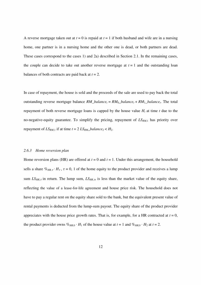

14
The one-period utility functions of the couple U is given by the equally weighted sum of the
husband and the wifersquos subutility functions Um and Uf (Brown and Poterba 2000)
678 9 = 58 ∙ 6878 9 + 59 ∙ 6979 8 (2-4)
6878 9 = ampBCDB
E)FGH
(I) (2-5)
6979 8 =ampB
EDBC)FGH
(I)
where 58 (59) is the indicator variable taking the value one if the husband (wife) is alive and 0
otherwise The parameter θ controls the degree of jointness (sharing of resources) in
consumption between the husband and the wife Both spouses have their subutility function
defined over consumption with an identical relative risk aversion parameter γ The bequest utility
function B exhibits the same relative risk aversion as U and is given by
=(1) = JBFGH
(I) (2-6)
The couplersquos objective is to maximize the expectation over (2-3) subject to a set of constraints
The couplersquos optimization problem is given by
maxBNOBPQCPQE PRSTUC PRSTUE EW0(1)X Y = 0 1 (2-7)
where the index j refers to cash flows from equity release schemes alternatively available
(j = RM HR) The optimization problem is subject to
(i) consumption and bequest constraints
15
A8 + A9 = 1A minus [A minus8 minus9 minus8 minus9 + [A
8 + 9 = [A ∙ (1 + ]A) minus [+$8 + $9 minus 71 minus+- minus8 ∙ 8 minus
71 minus+- minus9 ∙ 9 + [
Bequest constraint in case of the reverse mortgage
1 = [A ∙ (1 + ]A) + maxW minus _`_bcdcefg 0X
1 = [ ∙ (1 + ]) + maxW^ minus _`_bcdcefg 0X
Bequest constraint in case of the home reversion plan
1 = [A ∙ (1 + ]A) +71 minushiA ∙
1 = [ ∙ (1 + ]) + 71 minushiAminushi ∙ ^
(2-8)
(ii) borrowing constraints
0 le [A le 1A minus8 minus9 minus 8 minus 9 + [A (2-9)
0 le [ le [A ∙ (1 + ]A)+$8 + $9 minus 71 minus+- minus8 ∙ (8 + 138)
minus 71 minus+- minus9 ∙ (9+139) + [
(2-10)
(iii) no-short sale constraints for equity release and insurance products
0 le [A [ 8 9 8 9 (2-11)
and (iv) further product constraints
bull Maximum loan-to-value ratios for the reverse mortgage
[ikA le 0ikA8lm^A (2-12)
16
_`_bcdcefg + [ik le 0ik8lm
bull Maximum home reversion rate
hiAminushi le 1 (2-13)
bull LTCI benefits capped by actual care expenses
le 1 = (2-14)
28 Numerical Calibration of Baseline Parameters
This section describes the numerical calibration of the modelrsquos baseline parameters The
parameters are chosen to reflect the US market and to allow comparison with previous studies
Alternative parameter values are introduced in Section 3 Table 1 summarizes the numerical
calibration To distinguish product design effect from pricing effect especially in the different
equity release products all products are priced such that the product provider makes a zero
expected profit The pricing of the insurance and equity release products reflects the risks
inherent in these products
-- Table 1 here --
281 The Couplersquos Preferences and Endowment
The standard parameters for the couplersquos preferences (relative risk aversion subjective discount
factor strength of the bequest motive) are set within the range typically used in life cycle models
17
in the literature Relative risk aversion γ is set to 2 the subjective discount factor δ is set to 098
and the strength of the bequest motive β is set to 02 (see eg Laibson Repetto and Tobacman
1998 Cocco Gomes and Maenhout 2005 Inkmann Lopes and Michaelides 2011) The
jointness in consumption parameter θ is set to 02 This value is lower than the value of 05 used
by Brown and Poterba (2000) to reflect that jointness of consumption is less effective when one
or both partners are in a nursing home
The US HECM equity release program to which most reverse montages originated belong
requires both spouses to be at least 62 years old to access mortgages Thus the initial age of both
spouses is set to 62 at t = 0The maximum age in the model (at t = 2) is set to 100 and for having
identical period lengths the age at t = 1 is set to 81 making one period 19 years long The initial
endowment consists of liquid wealth of W0 = $135000 and a house worth H0 = $250000 which
reflect the median values for financial assets and primary residences for couples aged 60 to 65 in
the 2009 wave of the Survey of Consumer Finances
282 Interest Rates and House Price Growth
Interest rates are modeled as in Campbell and Cocco (2003) in their analysis of standard
mortgages That is future one-year interest rates are given by the mean rate plus a transitory iid
shock Based on one-year US Treasuries Campbell and Cocco estimate the mean of real
interest rates to be 2 with a standard deviation of 22 The interest rate over the first period
r0 is set equal to the mean real rate
18
Annual house price growth rates are modeled as normally distributed iid random variables The
parameters of the distribution are derived from estimates provided by Campbell and Cocco
(2003) based on the Panel Study of Income Dynamics (PSID) the mean real growth rate is 16
with a standard deviation of 1174
283 Health States Care Costs Long-Term Care Insurance and Annuity Products
For the calibration of the probabilities of the four health states (staying in good health needing
some care at home needing to move to a nursing home being death) and the state-dependent
care costs (0 moderate high 0) the same values are used as in Davidoff (2009) That is the
probabilities for entering the different states are based on Robinson (2002) and the annual care
expenses are based on Ameriks et al (2011) Annual care costs in real terms are $10000 in the
second state $50000 in the third state and zero otherwise LTCI for a 62 year old person is then
priced according to formula (2-1) with the interest rate of 2 Likewise annuities are priced
according to formula (2-2) using the respective survival probabilities A zero loading is assumed
for both the LTCI and annuities (LTCI = LTCI = 0)
284 Fair Pricing of the Reverse Mortgage
The reverse mortgage is priced such that provider of the product makes on average across all
future states a zero profit The profit is calculated as the expected present value of the loan
repayment (discounted using interest rates) minus the initial loan amount A margin ∆RM is
4 The total value of a house consists of the capital value and the rental yields The growth rate calibrated here is the
capital growth rate It excludes rental yields
19
determined that compensates the product provider for the equity guarantee (NNEG) embedded in
the reverse mortgage
Figure 2 gives the margin ∆RM0 for the variable interest rate reverse mortgage taken out at t = 0
for different actual loan-to-value ratios (LTVs) Given the calibration of interest rate house price
and health states the value of the house will always be enough to repay the loan for small LTVs
up to 030 For LTVs between 035 and 085 there are states where the NNEG becomes effective
and this reflects in a positive margin on the interest rate The margins vary between 005 and
186 These values fall into the range reported by Shan (2011) who reports that for US
HECM loans the lenderrsquos margin is typically between 1-2 For LTVs higher than 085 the
profit of the insurer is always negative on average independent of the margin and this
establishes a maximum LTV
-- Figure 2 here --
The pricing of the variable interest rate reverse mortgage offered at t = 1 is similar a margin
∆LS1 is determined to compensate the product provider for the NNEG The value of the NNEG
depends on how much the household has already borrowed at t = 0 on the house price growth
rate over the first period and on interest rates at t = 1 Figure 3 gives the margin ∆RM1 for
different loan amounts represented as ldquoadditional loan-to-value ratiordquo Results are presented for
20
different values of initial borrowing (ie for different LTVRM0 ratios) assuming low house price
growth over the first period and low interest rates over the second period
-- Figure 3 here --
285 Fair Pricing of the Sale and Lease Back Plan
The sale and lease back plan is priced such that product provider makes on average across all
future states a zero profit The providerrsquos profit is calculated as the expected present value of the
proceeds from sale of the equity share minus the initial lump sum paid out to the household This
initial lump sum is reduced to account for the expected present value of rental yields
To determine present values of sale proceeds and rental yields discount factors are used that
reflect house price risk The discount factors for the first period are determined by dividing the
total value of the ldquoreleasedrdquo equity share at t = 1 by the value of that share at t = 0 The total
value includes capital growth as described in Section 282 and rental yields over the first period
A discount factors for the second period is determined in the same way Rental yields over the
first and the second period are computed from an annual rental yield rent which is a percentage
of the equity share HRτ middot Hτ sold at the beginning of the period τ = 0 1
Previous studies on optimal consumption and portfolio choices have considered a rental yield of
6 per year (Yao and Zhang 2005) At this value and given the calibration of interest rate
house price and health states only 24 of the value of the equity share is paid out to the couple
21
under a home reversion plan taken out at t = 0 (and this value is independent of the percentage
HR that the couple decides to sell) In this study a lower (after-tax) rental yield of 2 is used
resulting in 54 of the value of the equity share paid out to the couple Alternatively a rental
yield of 4 is considered
286 Government-Provided Long-Term Care Insurance
With the government-provided LTCI the individual has to cover (1 minus+-) =50 of the
care costs up to a maximum of care costs of $6276 pa (equal to $100000 for the 19-year
horizon) For care costs higher than $6276 pa the individualrsquos out-of-pocket costs are limited
to 50$6276 pa
3 Results
The MATLAB function fmincon was used to implement the couplersquos optimization problem as a
constrained nonlinear optimization problem For the numerical solution of the model the house
price process is discretized using a binomial process (as in Yao and Zhang 2005 or Davidoff
2010c) The interest rate process is discretized in the same way
31 Optimal Equity Release at Different Points in Time
The base case is when the couple decides on consumption saving on purchasing annuities
private long-term care insurance (LTCI) and on taking out an equity release product The model
parameters are the baseline parameters given in Table 1 Different scenarios are compared One
22
scenario without equity release products two scenarios in which either the reverse mortgage or
the home revision plan described in Section 26 are offered only at t = 0 and two scenarios in
which the reverse mortgage or the home revision plan are offered at t = 0 and t = 1
Government-provided LTCI is not available in any of the five scenarios Table 2 gives the
corresponding results
-- Table 2 here --
The results for first three scenarios show that the couple clearly has a demand for equity release
products at time t = 0 When offered the reverse mortgage only at t = 0 the couple chooses to
borrow up to the maximum loan-to-value-ratio (LTV) When offered the home reversion plan at
t = 0 the household chooses to convert a very large proportion HR0 of the home In both cases
the changes in expected discounted utility indicate substantial welfare gains for the couple The
utility gain is higher for the reverse mortgage than for the home reversion plan
Having access to equity release products at time t = 1 in the last two scenarios further improves
the couplersquos utility but the utility gain is smaller than the utility gain from having access to
equity release products at t = 0 Borrowing and home reversion mainly takes place at t = 0
Table 2 reports the couplersquos consumption annuity premiums LTCI premiums and savings at
t = 0 as percentages of initial liquid wealth W0 before equity release The sum of these figures
23
indicates that the couple significantly increases their liquid wealth with equity release products
The reverse mortgage results in higher lump-sum payments which explains why this product is
preferred over the home reversion plan The additional liquidity from the two equity release
products is used to increase consumption C0 and to increase savings Annuity demand is
relatively stable across scenarios It is low because the annuity pays only at t = 1 and because of
the bequest motive Private LTCI demand is also unchanged The couple faces uncertain but
potentially high care costs and always buys full LTCI coverage as a result
32 Government-Provided Long-Term Care Insurance
Next a variant of the model with compulsory government-provided LTCI as described in
Sections 25 and 286 is considered Again the couple decides on consumption saving on
purchasing annuities private long-term care insurance (LTCI) for the remaining out-of-pocket
care costs and on equity release The model parameters are the baseline parameters given in
Table 1 Three different scenarios are compared One scenario without equity release products
and two scenarios in which the reverse mortgage or the home revision plan described in Section
26 are offered at t = 0 and t = 1 The numerical results for these scenarios are given in Table 3
Scenarios with equity release products offered only at t = 0 are not compared separately
-- Table 3 here --
The couple benefits from the fairly generous government-provided LTCI scheme but the utility
gains are much smaller than the utility gains from having access to equity release products This
24
can be seen by comparing the scenario without equity release products in Table 3 with the base
case results presented in Table 2 in the previous section
Similar levels of equity release are found to be optimal with the government-provided LTCI As
in the base case without public LTCI the couple chooses to borrow up to the maximum loan-to-
value-ratio (LTV) of the reverse mortgage at t = 0 and similar levels of home reversion at t = 0
and t = 1 are found to be optimal
With the government-provided LTCI the couple spends less of their wealth on private LTCI
They still choose to buy full coverage for each partner but because the private insurance only
covers the remaining out-of-pocket care costs the premiums are much lower They use the
additional wealth to buy more annuities
33 Sensitivity Analyses Higher Risk Aversion No Bequest Motive and a Higher House
Value
Table 4 gives the results for three different cases used to test the sensitivity of the base case
results presented in Table 2 in Section 31 In each case one model parameter is varied The first
case is when the couple has no bequest motive (β = 0) in the second case a higher risk aversion
is assumed (χ = 5) and in the third case a higher initial house value of H0 = $500000 is
considered For each case three different scenarios are compared One scenario without equity
25
release products and two scenarios in which the reverse mortgage or the home revision plan
described in Section 26 are offered at t = 0 and t = 1
-- Table 4 here --
In the case without a bequest motive the couple decidesmdashas in the base casemdashto borrow the
maximum loan-to-value-ratio (LTV) allowed with the reverse mortgage at t = 0 When offered
the home reversion plan at t = 0 and at t = 1 they choose to sell their home completely at t = 0
(HR0=100) in exchange for a lump-sum payment and a lease-for-life agreement Without a
bequest motive the couple buys significantly more annuities in all three scenarios than in the
base case with a bequest motive which is in line with the findings of previous studies (Brown
and Poterba 2000) Private LTCI demand is largely unaffected the couple chooses full coverage
for each partner
The middle columns of Table 4 refer to the case when the couple has a higher risk aversion than
in the base case (γ = 5 instead of γ = 2) Again as in the base case the couple decides to borrow
the maximum loan-to-value-ratio (LTV) allowed with the reverse mortgage at t = 0 The home
reversion pattern is different from the base case in Section 31 being more risk averse the
couple decides to release more of their home equity at t = 0 and less at t = 1 (HR0=80 and
HR1=18 compared to 75 and 14 in the base case) The couple buys significantly more
26
annuities in all three scenarios than in the base case but their decision to fully insurance long-
term care costs with private LTCI is unchanged
In the third case presented in the last three columns of Table 4 a higher initial house value of
H0 = $500000 is considered In the base case the house value H0 = $250000 made up 65 of
the couplersquos total wealth at t = 0 This ratio is 79 for a house value H0 = $500000 The results
show that the couple chooses to borrow a similar amount with the reverse mortgage although the
loan-to-value ratios both at t = 0 and at t = 1 are reduced More equity than in the base case is
released with the home reversion scheme
Three key findings emerge across the cases with alternative parameter values (no bequest
motive higher risk aversion and in higher initial house value) and these findings are consistent
with the base case (i) The couple has large utility gains from having access to either one of the
two equity release products (ii) higher utility gains are found for the reverse mortgage and (iii)
equity release predominantly takes place at t = 0
4 Summary and Conclusions
This study models the decision problem of a retiring couple that holds the major fraction of their
wealth as home equity and faces longevity risk long-term care risk house price risk and interest
rate risk The couple can choose to buy annuities long-term care insurance and to borrow
against the home using different equity release products at different point in time The numerical
27
results of this study suggest that the couple enjoys large utility gains from having access to either
one of the two equity release products Higher utility gains are found for the reverse mortgage
The household chooses to unlock home equity early on in retirement The key results are
consistent across a range of cases with different parameter values The availability of a
government-provided LTCI does not change the use of equity release products significantly but
does change the demand for annuities
References
Ameriks J A Caplin S Laufer and S Van Nieuwerburgh (2011) The Joy of Giving or
Assisted Living Using Strategic Surveys to Separate Bequest and Precautionary Motives
Journal of Finance 66 519ndash561
Andrews D and A Caldera Saacutenchez (2011) Drivers of Homeownership Rates in Selected
OECD Countries OECD Economics Department Working Papers No 849 OECD
Publishing
Artle R and P Varaiya (1978) Life cycle consumption and homeownership Journal of
Economic Theory 18 38ndash58
Australian Securities and Investments Commission (2005) Report 59 - Equity release products
November 2005
Brown J R and A Finkelstein (2007) Why is the market for long-term care insurance so
small Journal of Public Economics 91 1967ndash1991
Brown J R and J M Poterba (2000) Joint Life Annuities and Annuity Demand by Married
Couples Journal of Risk and Insurance 67 527ndash553
Campbell J Y and J F Cocco (2003) Household Risk Management and Optimal Mortgage Choice
Quarterly Journal of Economics 118 1449ndash1494
Case K J Cotter and S Gabriel (2011) Housing Risk and Return Evidence from a Housing
Asset-Pricing Model Journal of Portfolio Management 35 89ndash109
28
Cocco J F F J Gomes and P J Maenhout (2005) Consumption and Portfolio Choice Over
the Life-Cycle Review of Financial Studies 18 491ndash533
Davidoff T (2009) Housing Health and Annuities Journal of Risk and Insurance 76 31ndash52
Davidoff T (2010a) Financing Retirement with Stochastic Mortality and Endogenous Sale of a
Home Working Paper
Davidoff T (2010b) Home equity commitment and long-term care insurance demand Journal
of Public Economics 94 44ndash49
Davidoff T (2010c) Interest Accumulation in Retirement Home Equity Products Working
paper University of British Columbia
Davidoff T and G Welke (2006) Selection and Moral Hazard in the Reverse Mortgage
Market Working paper University of CaliforniandashBerkeley
Deloitte and SEQUAL (2012) Australiarsquos reverse mortgage market reached $33bn at 31
December 2011 Media Release 5 June 2012
Commission on Funding of Care and Support (2011) Fairer Care Funding ndash The Report of the
Commission on Funding of Care and Support July 2011 available at
httpwwwdilnotcommissiondhgovuk
Fratantoni M C (1999) Reverse Mortgage Choices A Theoretical and Empirical Analysis of
the Borrowing Decisions of Elderly Homeowners Journal of Housing Research 10 189ndash
208
Inkmann J P Lopes and A Michaelides (2011) How Deep is the Annuity Market
Participation Puzzle Review of Financial Studies 24 279ndash319
Koijen R S J S Van Nieuwerburgh and M Yogo (2011) Health and Mortality Delta
Assessing the Welfare Cost of Household Insurance Choice Netspar Discussion Paper No
052011-050
KRS Key Retirement Solutions (2011) UK Equity Release Market Monitor 2010 Review
Laibson D I A Repetto and J Tobacman (1998) Self-Control and Saving for Retirement
Brookings Papers on Economic Activity 1998 91ndash196
Mitchell O S J M Poterba M J Warshawsky and J R Brown (1999) New Evidence on the
Moneyrsquos Worth of Individual Annuities American Economic Review 89 1299ndash1318
29
Oliver Wyman (2008) Moving beyond HECM in equity release markets available at
httpwwwoliverwymancomdeu-insightsOliver_Wyman_-
_Moving_beyond_HECM_in_equity_release_marketspdf
Productivity Commission (2011) Caring for Older Australians ndash Productivity Commission
Inquiry Report No 53 28 June 2011 available at
httpwwwpcgovauprojectsinquiryaged-care
Reifner U S Clerc-Renaud E F Perez-Carillo A Tiffe and M Knoblauch (2009) Study on
Equity Release Schemes in the EU Part 1 General Report Hamburg
httpwwweurofinasorguploadsdocumentspoliciesequity_release_part1_enpdf
Robinson J (2002) A Long-Term Care Status Transition Model Working paper University of
Wisconsin
Shan H (2011) Reversing the Trend The Recent Expansion of the Reverse Mortgage Market
Real Estate Economics 39 743ndash768
Whitehead C and J Yates (2010) Is there a Role for Shared Equity Products in Twenty-First
Century Housing - Experience in Australia and the UK In S J Smith B A Searle (eds)
The Blackwell Companion to the Economics of Housing The Housing Wealth of Nations
Chichester Wiley-Blackwell
Yao R and H H Zhang (2005) Optimal Consumption and Portfolio Choices with Risky
Housing and Borrowing Constraints Review of Financial Studies 18 197ndash239
Yogo M (2009) Portfolio Choice in Retirement Health Risk and the Demand for Annuities
Housing and Risky Assets NBER Working Paper 15307
30
Table 1 Model Parameters
Parameter Baseline Value Alternative Value
House value t = 0 H0 $250000 $500000 Liquid wealth t = 0 W0 $135000 Age of both spouses t = 0 in years 62
Relative risk aversion γ 2 5 Subjective discount factor δ 098 Jointness of consumption θ 05
Strength of bequest motive β 02 0 Long term care expenses per year LTC
i $10000 (needing some
care at home) $50000 (needing care in a
nursing home)
Mean interest rate per year (= interest rate at t = 0)
r0 20
Standard deviation of interest rate per year
Std(r0) 22
Mean house price growth per year g 16 Standard deviation of house price growth per year
Std(g) 117
Rental yield 2 4 Mortgage rate margin per year mo 0 175 Annuity loading factor λA 0 10
Long term care insurance loading factor
λLTCI 0 16
Coinsurance percentage of the govt-provided LTCI
+- 50
Stop loss of the govt-provided LTCI per year
$6276
Notes This table shows baseline and alternative model parameters All parameters referring to multiple years (subjective discount factor interest rate house price growth mortgage rate) are scaled by the period length (19 years) in the model All monetary values are in real terms
31
Table 2 Optimal Equity Release at Different Points in Time
No Equity Release Products
Reverse Mortgage at
t = 0
Home Reversion at
t = 0
Reverse Mortgage at
t = 0 and t = 1
Home Reversion at
t = 0 and t = 1
Financial decisions at t = 0
Consumption 51 127 141 148 104
Annuity premiums 19 18 28 18 16
LTCI premiums 21 21 21 21 21
Savings 10 92 1 70 34
Sum 100 257 190 257 174
LTCI coverage 100 100 100 100 100
LTV0
85
85 HR0
91
75
Financial decisions at t = 1
Consumption 13 25 77 29 57
Savings 3 75 18 71 73
Sum 16 100 95 100 130
LTV1
0 HR1
14
Expected discounted utility -781E-05 -438E-05 -479E-05 -416E-05 -464E-05
Notes RM denotes the lump-sum reverse mortgage with variable interest rates and a no-negative-equity guarantee HR denotes the home reversion plan All variables are given at the household level summing husbandrsquos and wifersquos values Consumption annuity premiums LTCI premiums and savings at t = 0 are reported as percentages of liquid wealth W0 at t = 0 before equity release Consumption and savings at t = 1 are reported as percentages of liquid wealth at time t = 1 before additional equity release
32
Table 3 The Impact of Government-Provided LTCI on Optimal Equity Release
No Equity Release Products
Reverse Mortgage at t = 0 and t = 1
Home Reversion at t = 0 and t = 1
Financial decisions at t = 0
Consumption 74 148 117
Annuity premiums 22 37 27
LTCI premiums 4 4 4
Savings 0 68 21
Sum 100 257 169
LTCI coverage 100 97 98
LTV0
85 HR0
70
Financial decisions at t = 1
Consumption 12 40 72
Savings 7 59 65
Sum 19 99 137
LTV1
0 HR1 14
Expected discounted utility -627E-05 -319E-05 -394E-05
Notes All variables are given at the household level summing husbandrsquos and wifersquos values Consumption annuity
premiums LTCI premiums and savings at t = 0 are reported as percentages of liquid wealth W0 at t = 0 before equity
release Consumption and savings at t = 1 are reported as percentages of liquid wealth at time t = 1 before
additional equity release
33
Table 4 Sensitivity Analyses Higher Risk Aversion No Bequest Motive and a Higher House Value
No bequest motive (β = 0) Higher risk aversion (χ = 5) Higher house value (H0 = $500000)
No Equity Release Products
Reverse Mortgage
at t = 0 and t = 1
Home Reversion at t = 0 and
t = 1
No Equity Release Products
Reverse Mortgage
at t = 0 and t = 1
Home Reversion at t = 0 and
t = 1
No Equity Release Products
Reverse Mortgage
at t = 0 and t = 1
Home Reversion at
t = 0 and t = 1
Financial decisions at t = 0
Consumption 46 170 133 50 119 95 55 147 165
Annuity premiums 33 47 45 29 34 29 17 74 11
LTCI premiums 21 20 21 21 21 21 21 21 21
Savings 0 20 0 0 84 35 8 0 62
Sum 100 257 199 100 257 179 100 241 258
LTCI coverage 100 96 100 100 100 100 100 100 100
LTV0 85 85 38
HR0 100 80 83
Financial decisions at t = 1
Consumption 95 55 92 91 48 66 69 93 40
Savings 5 44 1 9 52 66 32 13 86
Sum 100 99 94 100 100 132 101 105 127
LTV1 0 0 3
HR1 0 18 10
Expected discounted utility -734E-05 -311E-05 -331E-05 -255E-19 -971E-21 -265E-20 -742E-05 -266E-05 -349E-05
Notes All variables are given at the household level summing husbandrsquos and wifersquos values Consumption annuity premiums LTCI premiums and savings at
t = 0 are reported as percentages of liquid wealth W0 at t = 0 before equity release Consumption and savings at t = 1 are reported as percentages of liquid
wealth at time t = 1 before additional equity release
34
Figure 1 Model Timing
Figure 2 Zero-profit margin for a reverse mortgage taken out at t = 0
Notes This graph shows the margin ∆LS1 for a variable interest rate reverse mortgage taken out at t = 0 for different
actual loan-to-value ratios
t = 0 Period 1 t = 1 Period 2 t = 2
Realization of random
- Health status of husband and wife
- House value
- Interest rate
rarr Borrow against home
rarr Buy annuity
rarr Buy LTCI
rarr Consume and save
rarr If both are dead bequeath net assets
rarr Else
rarr Receive annuity and LTCI payments
rarr Receive accumulated savings
rarr Borrow against home
rarr Cover out-of-pocket care costs
rarr Consume and save
rarr Bequeath net assets
Husband and wife are in
good health
Husband and wife die
Realization of random house value
35
Figure 3 Zero-profit margin for a reverse mortgage taken out at t = 1
Notes This graph shows the margin ∆LS1 for a variable interest rate reverse mortgage taken out at t = 1 The margin differs according to how much the household borrowed at t = 0 Results are given for different values of initial borrowing (ie for different LTVLS0 ratios) and refer to cases with low house price growth over the first period and low interest rates over the second period
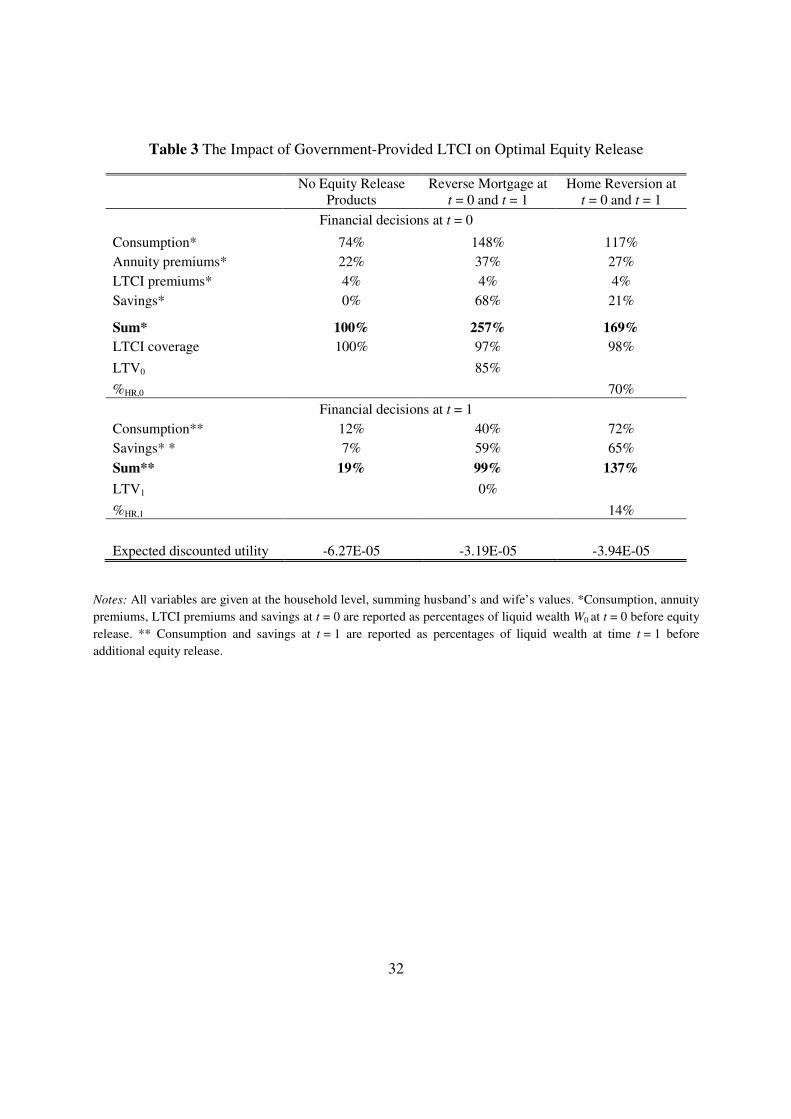