rising skill premium?: the roles of capital-skill
TRANSCRIPT

Rising Skill Premium?: The Roles of Capital-Skill Complementarity and Sectoral Shifts in a Two-Sector Economy Naoko Hara* [email protected] Munechika Katayama** [email protected] Ryo Kato*** [email protected]
No.14-E-9 October 2014
Bank of Japan 2-1-1 Nihonbashi-Hongokucho, Chuo-ku, Tokyo 103-0021, Japan
* Research and Statistics Department ** Kyoto University *** Research and Statistics Department (currently Monetary Affairs Department)
Papers in the Bank of Japan Working Paper Series are circulated in order to stimulate discussion and comments. Views expressed are those of authors and do not necessarily reflect those of the Bank. If you have any comment or question on the working paper series, please contact each author.
When making a copy or reproduction of the content for commercial purposes, please contact the Public Relations Department ([email protected]) at the Bank in advance to request permission. When making a copy or reproduction, the source, Bank of Japan Working Paper Series, should explicitly be credited.
Bank of Japan Working Paper Series

Rising Skill Premium?: The Roles of Capital-Skill Complementarity
and Sectoral Shifts in a Two-Sector Economy∗
Naoko HaraBank of Japan
Munechika KatayamaKyoto University
Ryo KatoBank of Japan
October 20, 2014
Abstract
Empirical studies report a marked dispersion in skill-premium changes across economiesover the past few decades. Structural models in early studies successfully replicate theincreases in skill premiums in many economies, while some other cases with a declinein the skill premium are yet to be explained. To this end, we develop a two-sector (i.e.,manufacturing and non-manufacturing) general equilibrium model with skilled andunskilled labor, in which degrees of capital-skill complementarity differ across sectors.Based on the estimated structural parameters, we show that a decline in capital-skillcomplementarity in the non-manufacturing sector can provide a consistent explanationfor the following aspects of the Japanese data at both the aggregate and industry levels:(i) a decline in the skill premium, (ii) widening of the sectoral wage gap due to a risein manufacturing wages and decline in non-manufacturing wages, and (iii) an increasein the unskilled labor share in the non-manufacturing sector. We interpret that thischange reflects compositional effects and uneven technology adoption of firms withinnon-manufacturing.
Keywords: Capital-skill Complementarity; Skill Premium; Two-sector DSGE Model;
Bayesian Estimation.
JEL Classification: E22, E24, J31;
∗We thank Kosuke Aoki, Seisaku Kameda, Michael Krause, Eiji Maeda, Shinichi Nishioka, staff of the Bank ofJapan, and conference/seminar participants at the Common Challenges in Asian and Europe, Asian Meeting ofEconometrics Society, Computing in Economics and Finance, Econometrics Society Australasian Meeting, andKyoto University for their helpful comments and suggestions. Views expressed here are those of the authors anddo not necessarily reflect those of the Bank of Japan.
1

1 Introduction
While the skill premium is generally thought to have been rising over time, a few economieshave actually seen skill premiums decline over the past decade. Among others, this paperfocuses on three notable aspects of the Japanese labor market at the industry level. First, theskill premium, defined as the ratio of the skilled wage to the unskilled wage, started to declinearound the mid-1990s. Second, while the average manufacturing wage has kept rising, thenon-manufacturing wage has declined significantly. Lastly, the input share of unskilled laborhas increased over time in the non-manufacturing sector while holding relatively steady formanufacturers. These changes observed in the Japanese economy are in sharp contrast towhat we have seen in most other economies. Understanding the main factors behind thesedifferences is likely to have quite important policy implications for economic growth.
This paper studies a two-sector general equilibrium model with two types of labor,skilled and unskilled, and aims to account for the aforementioned three observations ina neoclassical framework. In particular, we introduce capital-skill complementarity, suchthat the production technology exhibits complementarity between skilled labor and physicalcapital stock as discussed in Krusell et al. (2000). Parameter values are crucial for the degreeof capital-skill complementarity. We fit our two-sector DSGE model to quarterly sectoraldata, using Bayesian methods to estimate the key structural parameters. We then use ourmodel to perform a number of comparative statics exercises with a view to identifying themain driving force behind the aforementioned changes in the Japanese economy.
While the aggregate hourly wage started to decline in the mid-1990s, we observe starkdifferences in wages across the two sectors, i.e., manufacturing and non-manufacturing.More specifically, while the hourly wage in the manufacturing sector continues to rise overtime, the hourly wage in the non-manufacturing sector has declined since the mid-1990s. Asa result, the sectoral wage gap, measured by the relative wage, has widened by about 15percentage points since the mid-1990s. Meanwhile, the skill premium, which has typicallyincreased in other advanced economies as well as emerging nations, has decreased by about8.4 percentage points on average. We need a two-sector setup in order to illustrate the diver-gence of sectoral wages and the decrease in the skill premium within the same framework.If sectoral wages had not diverged, it would be possible to conclude that the aggregate wagehas merely been reflecting changes in productivity. Moreover, in one-sector models, thedecline in the skill premium can be simply attributed to skill-biased technological changes.1
These changes, however, cannot describe the difference in sectoral wages. Alternatively,Kawaguchi and Mori (2014) seek to offer some evidence for a labor-supply-side story toexplain changes in the wage gap between college and high school graduates.2 They pointout that increasing relative supply of college graduates would lead to a decline in the skill
1There exists a vast literature on the skill-biased technological change. See, for example, Acemoglu (2002).2The skill premium we will look at is different from the college premium they analyzed.
2
premium based on educational attainment. However, the aforementioned divergence ofsectoral wages implies that structural changes on the labor supply side are unlikely to be themain reason for the skill premium having declined, because such changes would affect bothmanufacturing and non-manufacturing proportionally.
In this paper, we show that changes in capital-skill complementarity in the non-manufacturingsector can explain the stylized facts. Since we primarily focus on structural changes in themanufacturing and non-manufacturing sectors, the labor supply side in our model has arelatively simple structure. We just take the existence of the two types of labor as givenand assume that households are indifferent between working for manufacturers or non-manufacturers. The two sectors hire both skilled and unskilled workers. Depending on thedegree of capital-skill complementarity, firms choose a different mix of skilled and unskilledworkers in terms of hiring.
Based on the estimated structural parameters, we find that a decline in the degree ofcapital-skill complementarity in the non-manufacturing sector can account for the observeddecline in the skill premium. Specifically, lower capital-skill complementarity arising froma reduction in the elasticity of substitution between capital and unskilled labor in the non-manufacturing industry provides a consistent explanation for the observed changes in theskill premium and sectoral wages as well as the increased share of unskilled labor in thenon-manufacturing sector.
We believe that the decline in capital-skill complementarity is consistent with what hasbeen occurring in the Japanese economy since the mid-1990s. In our two-sector model, wecan interpret a drop in the elasticity of substitution between capital and unskilled labor as aconsequence of the ongoing expansion of the unskilled labor intensive services sector, whichincludes food services and nursing care. Even though we cannot address this compositionaleffect within the non-manufacturing sector in this model, the increasing importance of theseindustries relative to traditional non-manufacturing industries can be reflected in the lowerelasticity of substitution between capital and unskilled labor.
The idea of capital-skill complementarity is not new. Griliches (1969) first hypothesizesthat skill or education is more complementary with physical capital than unskilled labor.Recently, Krusell et al. (2000) revive the idea of capital-skill complementarity, using it toaccount for the observed increases in the skill premium in the US economy at the aggregatelevel. Although the increase in the skill premium has typically been attributed to unobservedskill-biased technological changes, they argue that capital-skill complementarity helps ex-plain observed changes in the skill premium.3 Our paper is related to Maliar and Maliar(2011), who construct a general equilibrium version of Krusell et al. (2000), together withadditional driving forces. They derive restrictions that make the model consistent with bal-
3Polgreen and Silos (2008) re-examine findings of Krusell et al. (2000). They assure the existence of capital-skillcomplementarity. However, they also find that other results in Krusell et al. (2000) were sensitive to the dataused.
3

anced growth. In contrast, our model focuses on the two-sector setup around a detrendedsteady state.
We estimate the degree of sectoral capital-skill complementarity within a frameworkof business-cycle models by using quarterly time series data. While most existing studiesfocus on the long-run implications of capital-skill complementarity, there are a few excep-tions. Lindquist (2004) looks at a cyclical property of capital-skill complementarity. Hisfinding suggests that capital-skill complementarity is an important factor in explaining theskill premium over the business cycle. In terms of aggregate production technology, how-ever, Balleer and van Rens (2013) reach the opposite conclusion. They construct a quarterlyskill premium series for the US economy using the Current Population Survey and thenestimate responses of the economy to various technology shocks using a structural vectorautoregression framework. In particular, they find that the skill premium responds neg-atively to investment-specific technology shocks. Their finding rejects the possibility ofcapital-skill complementarity and favors the existence of capital-skill substitutability in theaggregate production technology. Our own empirical analysis indicates that there is a sig-nificant difference in the degree of capital-skill complementarity between the manufacturingand non-manufacturing industries. In fact, our comparative statics exercises suggest thatcapital-skill complementarity vanishes for non-manufacturers in Japan. This heterogene-ity of capital-skill complementarity might explain the conflicting results between Lindquist(2004) and Balleer and van Rens (2013).
Capital-skill complementarity is also increasingly important in the international tradeliterature. Parro (2013) develops a general equilibrium trade model with capital goods tradeand capital-skill complementarity. In this setup, he shows that there are two possibilitiesthat increase the skill premium. A technical change causes the relative price of capital todecline, which in turn increases the skill premium. This is true even in a closed economy. Inaddition, with capital goods trade, a decline in trade costs also reduces the price of capitalgoods, thereby catalyzing more trade in capital goods. As a result, the productivity ofskilled labor and the skill premium both increase when capital-skill complementarity exists.This result has an important welfare implication for the Japanese economy: if capital-skillcomplementarity weakens, it will become more difficult for the Japanese economy to enjoygains from trade (through cheaper capital goods with reduced transportation costs).
In terms of changes in sectoral allocation of labor, Ngai and Pissarides (2007) offer analternative explanation. They show that as long as goods and services are complements,labor will flow into a sector with lower TFP growth. Marquis and Trehan (2010) applythis idea to explain sectoral dynamics in the US economy, finding that the elasticity ofsubstitution between goods and services is zero or thereabout, and that labor thus flowsfrom manufacturing to services. However, our estimation results suggest that the elasticityof substitution between goods and services is not close to zero, and is indeed significantly
4

greater than unity.Apart from the concept of capital-skill complementarity and two types of labor, this paper
is related to Iacoviello et al. (2011), who use Baysian methods to construct and estimate a two-sector DSGE model. As with our own model, they make a clear distinction between goodsand services. Their model features a detailed structure of inventories in order to capturethe business cycle propagation mechanism. Two sectors (goods-producing and services-producing sectors) are differentiated by whether they hold inventories or not. This type ofdistinction is not included in our paper. Instead, the two sectors (i.e., goods and services)are different in our setup in terms of production technology, particularly with regard to thedegree of capital-skill complementarity.
The rest of the paper is organized as follows. Section 2 presents the stylized facts that wewould like to explain. Section 3 presents a two-sector neoclassical model with two types oflabor. In Section 4, we use Bayesian methods to estimate model parameters that are importantfor explaining the stylized facts. We then use the estimated parameters to conduct a numberof comparative statics exercises in Section 5. Section 6 concludes the paper.
2 Stylized Facts
Let us now present the stylized facts about the Japanese labor market that we would like toexplain. We will focus on the following three facts.
Fact 1 The skill premium has started to decline (at least over the last two decades, 2.45→ 2.3).
Fact 2 While the average hourly wage in the manufacturing sector has been increasing overtime, the non-manufacturing wage has been declining since the mid-1990s. As a result,the manufacturing to non-manufacturing wage ratio has increased quite sharply.
Fact 3 While the importance of part-time workers in the manufacturing industry has heldsteady, the percentage of total hours worked by part-time workers in the non-manufacturing industry has increased since the mid-1990s.
One important characteristic of the labor market is the distinction between skilled andunskilled workers. Let us now look at how the ratio of the skilled wage to the unskilled wage— the so-called “skill premium”— has evolved over time. Figure 1 shows the skill premiumsfor the manufacturing and non-manufacturing industries. Unlike in other economies, theskill premium has declined rather than rising over the past couple of decades. From 1993 to2012, the manufacturing and non-manufacturing skill premiums declined by 6.6% and 7.4%,respectively. Alternatively, we can look at an education-based measure. Parro (2013) uses thecollege/high-school graduates wage ratio and finds that the skill premium in Japan declinedby 3.4% from 1990 to 2005. This downward trend once again contrasts with other countries.
5

1994 1996 1998 2000 2002 2004 2006 2008 2010 20122.2
2.3
2.4
2.5
2.6
2.7
Manufacturing
Non−Manufacturing
Figure 1: Skill Premium
Note: The skill premium is defined as the ratio of the nominal hourly wage paid to full-time workers to that ofpart-time workers. We take our data from the Monthly Labour Survey of the Ministry of Health, Labour, andWelfare, focusing on the figures for establishments with five or more employees. Non-manufacturing excludesagriculture, forestry, fishery, and public administration sectors.
For example, the skill premium in Germany increased by 14.4% over the same period. In theUS, Parro (2013) finds that the skill premium as measured by the production/non-productionworkers wage ratio rose by 3.1% from 1990 to 2007. Moreover, he found that the skillpremium declined in just eight of the 28 countries analyzed. It is typically argued thatdemand for skilled workers should increase in advanced economies as a consequence oftrade with emerging economies and/or industrial off-shoring.4 As such, it would be naturalto expect the skill premium to rise over time. Since the literature has focused mostly on howto explain this upward trend, it is important to investigate why the skill premium has in factdeclined (or at best held steady) in Japan and a number of other economies.
In this paper, we view full-time workers as skilled labor, and we use part-time workers,whose scheduled work hours are shorter than for full-time workers at the same businessestablishment, as a proxy for unskilled labor. Part-time workers are suitable for the notionof unskilled workers, because tasks performed by part-time workers are typically limited toless skill-intensive ones. This classification is also advantageous in our estimation, becausewe can have longer monthly data series for part-time workers. An alternative measure of theskill premium is the college/high-school wage ratio, which is sometimes called the collegepremium. However, we cannot obtain any sufficiently long time-series data with quarterlyor higher frequency for the skill premium based on educational attainment. The collegepremium gives us qualitatively the same result as our measure based on full-time/part-time
4Since our model is a closed-economy model, we exclude a possible channel through international trade. Theprediction from the Stolper-Samuelson theorem is a decline in the skill premium in countries where unskilledlabor is abundant. It is difficult to say that Japan is a unskilled-labor-abundant country, relative to other countries.Thus, there is no harm in excluding the international trade channel.
6

1990 1995 2000 2005 20100
5
10
15
20
Non−Regular
Part−Time
Figure 2: Fraction of Non-Regular/Part-Time Jobs in College-Graduate Employments (%)Note: Data are taken from the Employment Status Survey conducted by the Statistics Bureau of Japan in 1987,1992, 1997, 2002, 2007, and 2012. We calculate the fraction of non-regular workers among college-graduateemployees (excluding executives) and that of part-time workers (including temporary workers). For 1987 and1992, we do not know the number of executives, but based on the average fraction for other years we assumethat 10% of total college-graduate employees are executives.
workers.Figure 2 provides some justification for not using college/high-school graduates to classify
skilled and unskilled workers. It shows the fraction of college-graduate workers who areclassified as non-regular workers (solid line) or part-time (including temporary) workers(dashed line). It is clear that there is an increasing tendency for college graduates to workin less skill-intensive jobs. These non-regular or part-time jobs usually involve routine tasksand do not pay well. If we use college/high-school graduates as proxies for skilled/unskilledworkers, we may overestimate the size of the skill premium. We acknowledge that regularworkers include those who may not be skilled. However, we believe that treating part-timeworkers as a proxy for unskilled workers is more suitable in our context, particularly oncedata availability is taken into account.
Figure 3a shows the nominal hourly wage at the aggregate level together with the sectoraldata.5 Wages increased for both the manufacturing and the non-manufacturing sectors untilthe mid-1990s. More recently, however, while the manufacturing wage has kept rising (albeitat a somewhat slower pace), the non-manufacturing wage has started to decline. Since thenon-manufacturing sector accounts for about 75% of all workers, this decline in the non-manufacturing wage has dragged down the aggregate hourly wage. This phenomenon istypically referred to as “wage deflation”.
5See the note to Figure 3 for a description of the data and the definitions of the manufacturing and non-manufacturing industries.
7

1980 1990 2000 2010
1.4
1.6
1.8
2
2.2
2.4
2.6
Aggregate
Manufacturing
Non−Manufacturing
(a) Nominal Wage (1,000 Yen)
1980 1990 2000 20100.9
0.95
1
1.05
1.1
1.15
(b) Manufacturing to Non-Manufacturing WageRatio
Figure 3: Nominal Wage Data
Note: We calculate the nominal hourly wage by dividing the total monthly wage bill (including overtime andbonuses) by the total hours worked in the month (including overtime hours). Where available, we use thedata on establishments with five or more employees. Prior to 1989, however, we extrapolate from the data onestablishments with 30 or more employees. Non-manufacturing does not include agriculture, forestry, fishing,and public administration. The data are obtained from the Monthly Labor Survey of the Ministry of Health,Labour and Welfare.
Figure 3b shows the ratio of the manufacturing wage to the non-manufacturing wage. Itcan be seen that this ratio was stable until the mid-1990s, but then started to rise sharply. Ifthis wage deflation were accompanied by deflation of general prices, we would not observethe aforementioned divergence of sectoral wages. As such, it is very important to look atthe sectoral data to understand the nature of aggregate wage deflation. The gap has in factwidened by about 15 percentage points over the past couple of decades or so.
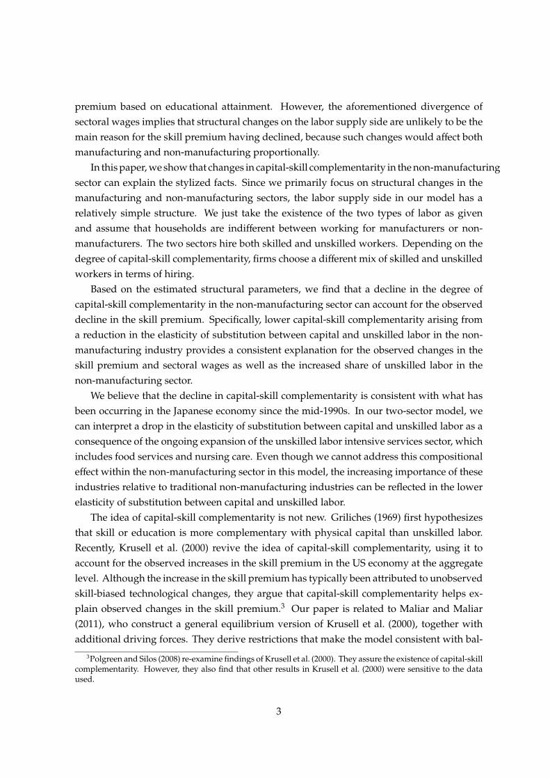
Figure 4 shows the unskilled labor shares for the manufacturing and non-manufacturingsectors. Again, we use hours worked by part-time workers as a proxy for unskilled labor.While the share of unskilled workers has held relatively steady in the manufacturing sector,it has been increasing over time for non-manufacturers. Krusell et al. (2000) report that thelabor input ratio of skilled to unskilled has been increasing in the US data since the 1960s.Meanwhile, the skill premium has increased drastically, especially from the 1980s to the1990s. These two findings are the opposite of what we see in the Japanese economy.
In the next section, we will present a model that can explain these three stylized facts inthe context of the Japanese economy.
8
1994 1996 1998 2000 2002 2004 2006 2008 2010 20125
10
15
20
25
Aggregate
Manufacturing
Non−Manufacturing
Figure 4: Fraction of Total Hours Worked by Part-time Workers (%)Note: The data are taken from the Monthly Labour Survey of the Ministry of Health, Labour, and Welfare. We usethe figures for establishments with five or more employees. Non-manufacturing excludes agriculture, forestry,fishing, and public administration. We divide the total hours worked by part-time workers by those worked byall (full-time and part-time) workers.
3 The Model
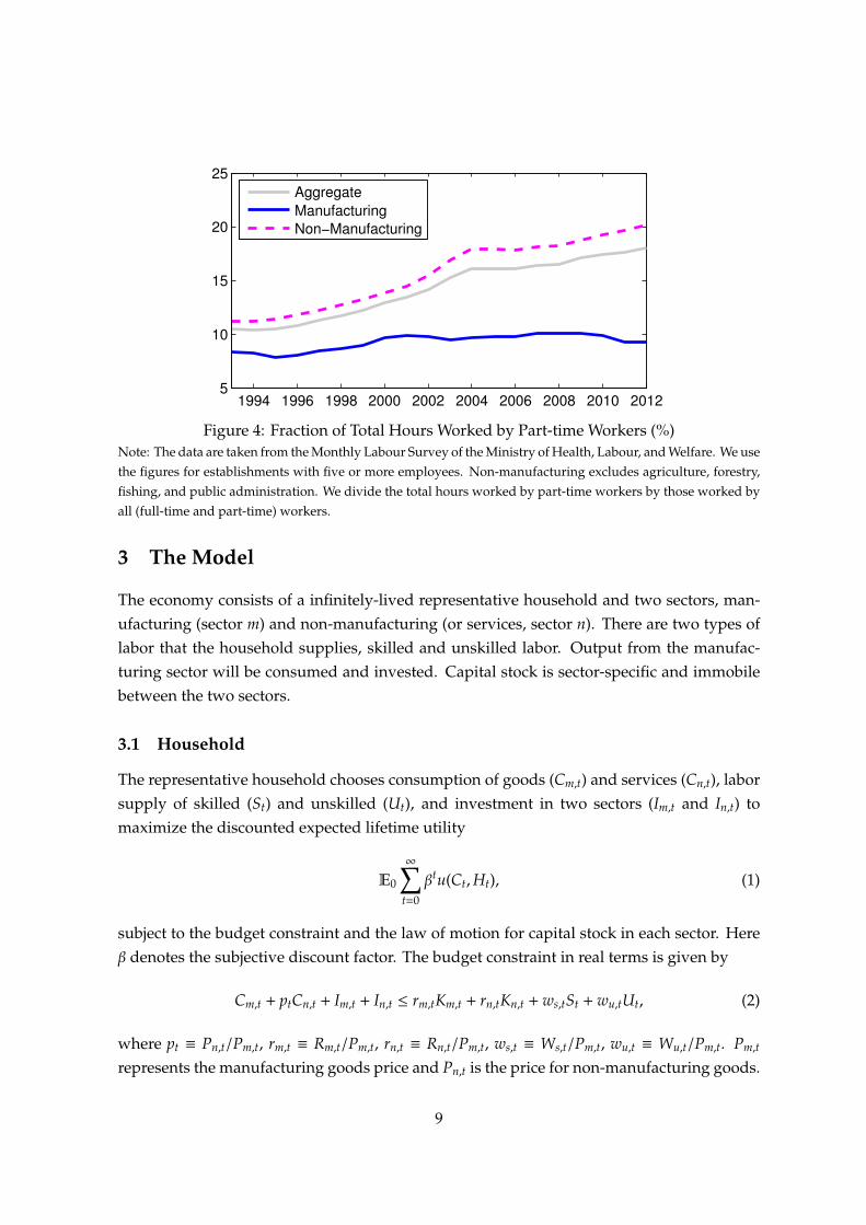
The economy consists of a infinitely-lived representative household and two sectors, man-ufacturing (sector m) and non-manufacturing (or services, sector n). There are two types oflabor that the household supplies, skilled and unskilled labor. Output from the manufac-turing sector will be consumed and invested. Capital stock is sector-specific and immobilebetween the two sectors.
3.1 Household
The representative household chooses consumption of goods (Cm,t) and services (Cn,t), laborsupply of skilled (St) and unskilled (Ut), and investment in two sectors (Im,t and In,t) tomaximize the discounted expected lifetime utility
E0
∞∑t=0
βtu(Ct,Ht), (1)
subject to the budget constraint and the law of motion for capital stock in each sector. Hereβ denotes the subjective discount factor. The budget constraint in real terms is given by
Cm,t + ptCn,t + Im,t + In,t ≤ rm,tKm,t + rn,tKn,t + ws,tSt + wu,tUt, (2)
where pt ≡ Pn,t/Pm,t, rm,t ≡ Rm,t/Pm,t, rn,t ≡ Rn,t/Pm,t, ws,t ≡ Ws,t/Pm,t, wu,t ≡ Wu,t/Pm,t. Pm,t
represents the manufacturing goods price and Pn,t is the price for non-manufacturing goods.
9

Rm,t and Rn,t are the rental rates for capital stock. Ws,t and Wu,t denote nominal wages forskilled and unskilled labor, respectively. The law of motion for capital stock in each sectorj = m,n is subject to investment adjustment costs Φ(·) and given by
K j,t+1 = I j,t
{1 −Φ
(I j,t
I j,t−1
)}+ (1 − δ)K j,t. (3)
Following Horvath (2000), we assume that the aggregate labor index takes the followingform:
Ht =[(St)
θ+1θ + (Ut)
θ+1θ
] θθ+1, (4)
where St and Ut represent skilled and unskilled labor, respectively. θ controls the elasticity ofsubstitution between skilled and unskilled jobs. Asθ→∞, skilled and unskilled jobs becomeperfect substitutes. Thus, if the skilled job pays a higher wage, the household allocates allof its labor supply to that job. On the other hand, when θ → 0, there is no way to changethe composition of the two types of jobs, so that skilled and unskilled jobs become perfectcomplements. In the somewhat more realistic case where 0 < θ < ∞, the household prefersto have diversity of labor. It is therefore possible for the household to supply both types oflabor even when the nominal wages offered for skilled and unskilled labor are different. Webelieve that this assumption is reasonable. This is the most parsimonious way to introduceskilled and unskilled labor into the representative agent framework.6 For example, Kondoand Naganuma (2014) find that skill difference is an important factor affecting inter-industrylabor flows in Japan. This specification may be viewed as a parsimonious way of describingjob polarization.
The composite consumption good Ct, which aggregates manufacturing goods and ser-vices, is defined similarly as
Ct =[γ(Cm,t
) κ−1κ + (1 − γ)
(Cn,t
) κ−1κ
] κκ−1, (5)
where γ ∈ [0, 1] is the share of the manufacturing good and κ is the elasticity of substitutionbetween manufacturing goods and services. As κ → 1, Ct = Cγm,tC
1−γn,t . As κ → ∞, Ct =
γCm,t + (1 − γ)Cn,t.For simplicity, we assume separability between aggregate consumption and labor. A
parametric form of the household preferences is given by
u(Ct,Ht) = log(Ct) − ϕη
1 + ηH
η+1η
t , (6)
6Alternatively, we could introduce sector-specific skills, such as skilled and unskilled workers in manufactur-ing and those in non-manufacturing, and corresponding sector-specific skill-biased technology shocks. However,the ratio of skilled wages paid in manufacturing and non-manufacturing has been stable. The same applies tothe unskilled wages. Thus, we believe that there is no harm in assuming that the labor market is not segmentedacross sectors.
10
where η is the Frisch elasticity of aggregate labor supply.
3.2 Firms
There are two types of firms in the economy, manufacturing (sector m) and non-manufacturing(sector n). A representative firm in each sector takes factor prices as given and maximizes itsprofits period by period.
We assume that production technology exhibits capital-skill complementarity as in Krusellet al. (2000). For each sector j = m,n, sectoral output Y j,t is produced from the followingtechnology
Y j,t = A j,t
[µ j(ψu,tU j,t)σ j + (1 − µ j)
{λ j(K j,t)ρ j + (1 − λ j)(ψs,tS j,t)ρ j
}σ j/ρ j]1/σ j
, (7)
where A j,t represents sectoral productivity, and ψs,t and ψu,t measure quality of skilled andunskilled labor, respectively. µ j and λ j control the factor shares of unskilled labor and capital,respectively.
We assume exogenous processes that drive sectoral productivity, and skilled and un-skilled labor efficiency as follows:
log(A j,t) = (1 − ρA j) log(A j) + ρA j log(A j,t−1) + ε j,t, (8)
log(ψl,t) = (1 − ρψl) log(ψl) + ρψl log(ψl,t−1) + ηl,t, (9)
where ε j,t ∼ N(0, σ2A j
) and ηl,t ∼ N(0, σ2ψl
) for j = m,n and for l = s,u. Sectoral productivityand labor efficiency are assumed to be stationary with |ρA j | < 1 for j = m,n and |ρψl | < 1 forl = s,u. This assumption rules out the possibility of differences in productivity growth ratedriving sectoral shifts.
The elasticity of substitution between capital and unskilled labor, which measures how
changes in the relative price affect relative input, is given by1
1 − σ j. Similarly, the elasticity
of substitution between capital and skilled labor is1
1 − ρ j. As shown in Krusell et al. (2000),
when σ j > ρ j, there is capital-skill complementarity, meaning that capital is more substi-tutable with unskilled labor than with skilled labor. We define α j ≡ σ j − ρ j, which can beused to measure the degree of capital-skill complementarity in sector j. When σ j → 0 andρ j → 0, the typical Cobb-Douglas production function emerges as a special case:
Y j,t = A j,t(K j,t)(1−µ j)λ j(ψs,tS j,t)(1−µ j)(1−λ j)(ψu,tU j,t)µ j . (10)
11

3.3 The Rest of the Model
To clear labor markets for skilled and unskilled workers, the goods market, and the servicesmarket, we have the following market clearing conditions.
St = Sm,t + Sn,t (11)
Ut = Um,t + Un,t (12)
Ym,t = Cm,t + Im,t + In,t (13)
Yn,t = Cn,t (14)
We construct the sectoral wage for j = m,n as
w j,t = (1 − τ j,t)ws,t + τ j,twu,t, (15)
where τ j,t =U j,t
S j,t+U j,t.
4 Estimation
We next fit our model to the data to estimate the key parameters that determine the size ofcapital-skill complementarity (σ’s and ρ’s), together with other structural parameters. To thisend, we estimate the model structurally by using a Bayesian approach. In order to improveempirical fit, we will augment the model presented in Section 3 by introducing sector-specificinvestment-specific technology shocks and skill-specific wage markup shocks. All of theseshocks are assumed to follow standard AR(1) processes. By fitting our model to the data, wecan use the estimated structural parameters to gain insight into the true determinant of theobserved changes in the Japanese economy (our three “stylized facts”).
4.1 Data
In order to take advantage of our two-sector setup, we will utilize quarterly disaggregateddata. We assume that output from the manufacturing sector is used for durable goods pur-chases, business fixed investment, and residential investment. Similarly, non-manufacturingoutput is used for non-durable goods and services. It is quite difficult to make a clear distinc-tion between skilled and unskilled labor, especially at the quarterly frequency for sufficientlylong time periods. We construct our own measures for hours worked for skilled and un-skilled labor (with the latter proxied by part-time workers). Our Appendix explains the dataconstruction process in detail. Our sample starts from 1975:Q1 and ends at 1995:Q4. Our ob-jective is to configure our model parameters to provide a good representation of the Japaneseeconomy before the change we observe in the 1990s. This motivates us to pick 1995:Q4,
12
which roughly corresponds to the timing with which we start to observe the changes in thelabor market depicted in Figure 3, as the end of our sample.
We use the following data to estimate our model: the growth rate of manufacturingoutput (dym,t), the growth rate of non-manufacturing output (dyn,t), the growth rate of totalhours worked by full-time workers (dst), the growth rate of total hours worked by part-time workers (dut), the growth rate of the manufacturing wage (dwm,t), the growth rate ofthe non-manufacturing wage (dwn,t), and the inflation rate of the relative price betweenmanufacturing and non-manufacturing (dpt). The growth rates of output and hours workedare detrended by the growth rate of the population over 15 years of age.
We solve the log-linearized system of equations presented in Appendix B to get a state-space representation of the solution. It is then used to evaluate the log-likelihood functionwith the Kalman filter. Model variables that are expressed in terms of deviations fromthe steady state are linked to the data (all observable variables are demeaned) through theobservation equation as follows.
dym,t = ym,t − ym,t−1 (16)
dyn,t = yn,t − yn,t−1 (17)
dst = st − st−1 (18)
dut = ut − ut−1 (19)
dwm,t = wm,t − wm,t−1 (20)
dwn,t = wn,t − wn,t−1 (21)
dpt = pt − pt−1 (22)
4.2 Prior Distributions
As summarized in Table 1, we fix some parameter values and impose the steady-state ratiosin the estimation in order to maintain consistency with reality. We set the discount factor (β) tobe 0.995 and the depreciation rate (δ) to be 0.025. Based on the data, the manufacturing goodsexpenditure share (ωm) is set to be 0.25. We assume that the steady-state skill premium ws
wuis
2.45, which is consistent with the values seen in the early 1990s. We set the skilled-unskilledratio in manufacturing ( Sm
Um) to be 13.85 and that in non-manufacturing ( Sn
Un) to be 7.06. These
values are based on the average ratio of part-time workers to full-time workers over 1993–1995.7 Since the average labor income shares in manufacturing and non-manufacturingfrom 1980 to 1995 are 54% and 46%, respectively, we set the capital cost share parametersαkm = 0.46 and αkn = 0.54. Finally, we assume the manufacturing share of skilled workers
SmSm+Sn
to be 0.36. Through the steady-state relationship, we can infer other steady-state ratios
7Again, we do not have good data on the ratio of skilled to unskilled workers at the sectoral level for theearlier period.
13

Table 1: List of Parameter Values Imposed
Discount factor β = 0.995Depreciation rate δ = 0.025Goods expenditure share ωm = 0.25Skill premium π = 2.45Skilled-Unskilled ratio in sector m Sm
Um= 13.85
Skilled-Unskilled ratio in sector n SnUn
= 7.06Capital cost share in sector m αkm = 1 − 0.54Capital cost share in sector n αkn = 1 − 0.46Fraction of skilled in sector m fs = Sm
Sm+Sn= 0.36
Fraction of unskilled in sector m fu = fs(
wswu
)θ (SmUm
)−1
Share of skilled workers ωs = πθ+1
πθ+1+1
Share of unskilled in sector m ωum = (1 − αkm )(
wswu
SmUm
+ 1)−1
Share of unskilled in sector n ωun = (1 − αkn )(
wswu
SnUn
+ 1)−1
Share of capital in sector m ωkm =αkm
(1−ωum )Share of capital in sector n ωkn =
αkn(1−ωun )
Consumption share of goods ωc = (1 − ωim )(1 +
δαknrn
(1−ωm)ωm
)−1
Investment share of goods in sector m ωim =δαkm
rm
as summarized in Table 1.Table 2 summarizes the model parameters to be estimated, together with the associated
prior distributions. There are a couple of things we need to discuss. We use a Gammadistribution with mean 1.143 and standard deviation of 0.4 as the prior distribution for κ.This will give us its mode located at 1, which corresponds to Cobb-Douglas preferencesover Cm and Cn. Prior probability of κ < 1 is 40%. We consider this to be a much moreagnostic prior than that used in Iacoviello et al. (2011), for example. Whether the value of κis greater or less than unity is crucial for whether or not the data support the story of Ngaiand Pissarides (2007).
We assume that σ j for j = m,n is from a Beta distribution with mean and standarddeviation of 0.2. Our underlying assumption is that the elasticity of substitution betweencapital and unskilled labor is greater than or equal to unity. We define α j ≡ σ j − ρ j, whichcontrols the degree of capital-skill complementarity. We use a Gamma distribution withmean 0.5 and standard deviation 0.5 as the prior distribution for α j. This reflects our priorbelief that there exists capital-skill complementarity. We also allow for the possibility of nocapital-skill complementarity since the support of α j includes zero.
The remaining prior distributions are standard. The prior for the inverse Frisch laborsupply elasticity is the same as in Sugo and Ueda (2008). It is Normally distributed andcentered at 2 with standard deviation of 0.75. The prior for the investment cost parameterϕ is a Gamma distribution with mean 4 and standard deviation of 1. This is a widely
14

Table 2: Prior Distributions
PriorParameter Dist. Mean Std Devκ Elasticity of substitution between goods and services G 1.143 0.41η Inverse Frisch labor supply elasticity N 2 0.75σm Controlling the elasticity of substitution between Km and Um B 0.2 0.2σn Controlling the elasticity of substitution between Kn and Un B 0.2 0.2αm Controlling capital-skill complementarity in sector m G 0.5 0.5αn Controlling capital-skill complementarity in sector n G 0.5 0.5ϕ Investment adjustment cost parameter G 4 1ρam Persistence of TFP in sector m B 0.75 0.1ρan Persistence of TFP in sector n B 0.75 0.1ρψs Persistence of skilled-specific shock B 0.75 0.1ρψu Persistence of unskilled-specific shock B 0.75 0.1ρξm Persistence of investment-specific shock in sector m B 0.75 0.1ρξn Persistence of investment-specific shock in sector n B 0.75 0.1ρµs Persistence of wage markup shock for skilled B 0.75 0.1ρµu Persistence of wage markup shock for unskilled B 0.75 0.1σam Std Dev of TFP shock in sector m IG 0.025 ∞
σan Std Dev of TFP shock in sector n IG 0.025 ∞
σψs Std Dev of skilled-specific shock IG 0.025 ∞
σψu Std Dev of unskilled-specific shock IG 0.025 ∞
σξm Std Dev of investment-specific shock in sector m IG 0.025 ∞
σξn Std Dev of investment-specific shock in sector n IG 0.025 ∞
σµs Std Dev of wage markup shock for skilled IG 0.025 ∞
σµu Std Dev of wage markup shock for unskilled IG 0.025 ∞
Note: N, B, G, IG, and U stand for Normal, Beta, Gamma, Inverse Gamma, and Uniform distributions, respec-tively.
used prior for the investment adjustment cost parameter. The prior distributions for thepersistence parameters are all Beta distributions with mean 0.75 and standard deviation of0.1. We assume that the priors for the standard deviations of the structural shocks are allInverse Gamma distributions with mean 0.025. These choices are based on Iacoviello et al.(2011).
4.3 Results
Table 3 summarizes the posterior distributions of parameters estimated, which are generatedfrom 300,000 Metropolis-Hastings draws (the first 30,000 draws are discarded as burn-in). Weset the scaling parameter in the Metropolis-Hastings algorithm so that the average acceptancerate becomes about 30%. It is worth emphasizing a few things about our estimation results.
First, the elasticity of substitution between capital and unskilled labor differs substantiallybetween manufacturing and non-manufacturing. The posterior mean of σm is significantlygreater than zero and equal to 0.6254. The implied elasticity of substitution between capital
15

Table 3: Posterior Distributions
Posterior DistributionParameter Mean 90% Intervalκ Elasticity of substitution between goods and services 4.5705 3.7134 5.41861η Inverse Frisch labor supply elasticity 1.6710 1.1827 2.1474σm Controlling the elasticity of substitution between Km and Um 0.6254 0.5469 0.7011σn Controlling the elasticity of substitution between Kn and Un 0.0025 0.0000 0.0065αm Controlling capital-skill complementarity in sector m 4.5644 3.1990 5.8114αn Controlling capital-skill complementarity in sector n 0.4034 0.2879 0.5127ϕ Investment adjustment cost parameter 1.7129 0.7033 2.7524ρam Persistence of TFP in sector m 0.6618 0.5192 0.8116ρan Persistence of TFP in sector n 0.9490 0.9203 0.9803ρψs Persistence of skilled-specific shock 0.6645 0.5373 0.7920ρψu Persistence of unskilled-specific shock 0.7717 0.6699 0.8778ρξm Persistence of investment-specific shock in sector m 0.7558 0.5931 0.9222ρξn Persistence of investment-specific shock in sector n 0.9226 0.8746 0.9756ρµs Persistence of wage markup shock for skilled 0.9444 0.9127 0.9785ρµu Persistence of wage markup shock for unskilled 0.8059 0.7191 0.8928σam Std Dev of TFP shock in sector m 4.5705 3.7134 5.4186σan Std Dev of TFP shock in sector n 1.6710 1.1827 2.1474σψs Std Dev of skilled-specific shock 0.6254 0.5469 0.7011σψu Std Dev of unskilled-specific shock 0.0025 0.0000 0.0065σξm Std Dev of investment-specific shock in sector m 4.5644 3.1990 5.8114σξn Std Dev of investment-specific shock in sector n 0.4034 0.2879 0.5127σµs Std Dev of wage markup shock for skilled 1.7129 0.7033 2.7524σµu Std Dev of wage markup shock for unskilled 0.6618 0.5192 0.8116
Log Marginal Density 1548.90Note: Posterior distributions are generated from 300,000 Metropolis-Hastings draws. We discard the first
10% of draws as a burn-in period. We use the modified Harmonic mean estimator of Geweke (1999) toobtain the log marginal density.
and unskilled labor in manufacturing is 2.6696. This is much higher than the estimate inKrusell et al. (2000), which is obtained from the US aggregate data (1.67). On the other hand,the posterior mean of σn is quite small at just 0.0025. Moreover, the 90 percent probabilityinterval contains zero. The implied elasticity of substitution is very close to unity (1.0025).
Second, the degree of capital-skill complementarity is quite different between manufac-turing and non-manufacturing. The posterior mean of αm is 4.5644, suggesting that thereexists capital-skill complementarity in manufacturing. This implies that the estimated valueof ρm is −3.9390. The implied elasticity of substitution between capital and skilled labor inmanufacturing is 0.2025, which is much smaller than the estimate in Krusell et al. (2000) of0.67. The posterior mean of αn is 0.4034, which is much smaller than that in manufacturing,suggesting that ρn = −0.4009. The implied elasticity of substitution between capital andskilled labor in non-manufacturing is 0.7138, which is higher than in manufacturing, andstill lower than in the Cobb-Douglas case.
Third, the posterior mean of κ is 4.5705, which is significantly greater than unity. This
16

implies that goods and services are not complements, suggesting that the data do not supportthe story of Ngai and Pissarides (2007).
The TFP shock in manufacturing is less persistent (0.6618) than that in non-manufacturing(0.9490). The same pattern applies to the persistence of investment specific shocks (0.7558 inmanufacturing and 0.9226 in non-manufacturing). The skilled-specific shock is less persistentthan the unskilled-specific technology shock (0.6645 versus 0.7717). The opposite is true forwage markup shocks. While the persistence of the wage markup shock for skilled is estimatedto be 0.9444, that for unskilled is smaller at 0.8059.
5 Inspecting the Steady-State Skill Premium and Sectoral Wages
5.1 Steady-state Values and Comparative Statics
Based on the parameter estimates in Section 4, we perform comparative statics exercisesin order to understand factors behind the observed changes in the Japanese labor market.Alternatively, we could estimate our model with data for 1996 onwards to see what changesin the model parameters can account for the stylized facts. However, we think that might notbe an ideal way to explain changes in the labor market. First, it is possible that the Japaneselabor market is still in transition to a new steady state, in which case using the transitionperiod may give us somewhat misleading results. Second, it may be difficult to disentangleand identify the exact factor(s) accounting for the observed changes in the Japanese labormarket because it is highly likely that the data contain many structural factors affecting theJapanese economy during this time period. For these reasons, we believe that it is better totake a comparative statics approach.
We want the model to capture the key observed features of the Japanese economy prior tothe mid-1990s. We consider the size of the skill premium to be particularly important giventhat it characterizes the two different types of workers. Thus, we assume the steady-stateskill premium (ws/wu) to be 2.45, which roughly corresponds to the average skill premiumin the early 1990s. Together with the steady-state values of Um
Sm, Un
Sn, and Sn
Sm, the steady-state
skill premium satisfies ( ws
wu
)θ=
Sm
Um
(1 + Sn
Sm
)(1 + Un/Sn
Um/Sm
SnSm
) . (23)
We will choose the value of θ, such that we can hit the target ws/wu = 2.45. Since we haveimposed Um
Sm, Un
Sn, and Sn
Smin the estimation in the previous section, we can pin down the
value of θ. The skill-premium-consistent value of θ is 2.3978. Using the posterior means,we can obtain the share parameters µm and µn, γ, and the productivity level of unskilledrelative to skilled b ≡ ψu
ψs. To do this, we assume that the relative productivity level in
non-manufacturing AnAm
is unity, and we set λm = λn = 0.4.
17

0.5 0.6 0.7 0.82.2
2.4
2.6
2.8
3
ws/w
u
σm
−4.1 −4 −3.9 −3.82.4499
2.45
2.4501
2.4501
2.4501
ws/w
u
ρm
−0.1 0 0.1 0.22
2.5
3
3.5
ws/w
u
σn
−0.6 −0.5 −0.4 −0.32.435
2.44
2.445
2.45
2.455
2.46
ws/w
u
ρn
Figure 5: Changes in the Skill PremiumNote: The left panels depict changes in the skill premium (vertical axis) as σm and σn move. The right panelsillustrate changes in the skill premium as we vary ρm and ρn. The dashed vertical line denotes the posterior meanof the corresponding parameter.
0.5 0.6 0.7 0.8
0.35
0.4
0.45
0.5
0.55
0.6
0.65
Se
cto
ral W
ag
es
σm
−4.1 −4 −3.9 −3.80.46
0.47
0.48
0.49
0.5
Se
cto
ral W
ag
es
ρm
−0.1 0 0.1 0.20.4
0.45
0.5
0.55
Se
cto
ral W
ag
es
σn
−0.6 −0.5 −0.4 −0.30.47
0.475
0.48
0.485
0.49
0.495
Se
cto
ral W
ag
es
ρn
Wm
Wn
Figure 6: Changes in Sectoral WagesNote: The left panels depict changes in sectoral wages (vertical axis) as σm and σn move. The right panelsillustrate changes in sectoral wages as we vary ρm and ρn. The dashed vertical line denotes the posterior meanof the corresponding parameter.
18

Below we look at how the steady-state values change as we alter the values of σm, σn,ρm, and ρn, which are all relevant to the degree of capital-skill complementarity. An increasein σ means that the elasticity of substitution between capital and unskilled labor increases.Similarly, a rise in ρ translates into higher substitutability between capital and skilled labor.
Figure 5 depicts changes in the skill premium as we vary σ’s and ρ’s. The top left panelshows changes in the skill premium as σm moves and the bottom left figure corresponds tochanging σn. The top right plot illustrates changes in the skill premium with different valuesof ρm and the bottom right figure depicts how the skill premium varies as ρn changes. Thevertical dashed lines show the posterior mean of the corresponding parameter.
The skill premium becomes smaller as σ (σm or σn) decreases and/or as ρ (ρm or ρn)increases. In other words, reductions in the degree of capital-skill complementarity, σ−ρ, willdampen the skill premium. Why is this? With a lower degree of capital-skill complementarity,capital becomes more (less) substitutable with skilled (unskilled) labor than before. Thismeans that firms require a smaller amount of skilled labor to utilize their capital. If theskill premium is unchanged, there is an excess supply of skilled labor. Accordingly, the skillpremium decreases towards the level where there is no excess supply of skilled labor. Thus,any reduction in capital-skill complementarity (through one or any of σm, σn, ρm, and ρn)can lower the skill premium and is a candidate to explain the stylized facts mentioned inSection 2.8
Although changes in these parameters can explain the decline in the skill premium,inspecting Figure 6 reveals that changes in σm, ρm, and ρn cannot explain both changes inthe skill premium and the sectoral wages presented in Section 2. Figure 6 illustrates changesin sectoral wages as we move σ’s and ρ’s. As σm decreases, or as ρm and ρn increase,both manufacturing and non-manufacturing wages move in the same direction. This is notconsistent with the pattern observed in the data. Higher ρ’s induce sectoral wages to increase.Reductions in σm would lower both manufacturing and services wages. Since the speed ofreduction is slightly slower for the non-manufacturing wage, it could become higher thanthe manufacturing wage when the drop in σm is sufficiently large.
It is a decrease in σn that explains both the lower skill premium and the lower non-manufacturing wage. As σn decreases from the posterior mean, which is denoted by thevertical line in the figure, we can see that while the manufacturing wage increases slightly,the non-manufacturing wage declines considerably. This is consistent with what we haveobserved in the Japanese labor market since the mid-1990s.
Figure 7 compares changes in skilled and unskilled wages as we alter σ’s and ρ’s. Thesepictures indicate that skilled and unskilled wages move in the same direction as capital-skillcomplementarity in the manufacturing sector declines. On the other hand, the skilled wagedrops and the unskilled wage rises as capital-skill complementarity in non-manufacturing
8In our model, lower capital-skill complementarity might increase the skill premium if unskilled labor ac-counts for a majority of the labor market. However, this may not be the case for Japan.
19
0.5 0.6 0.7 0.80
0.2
0.4
0.6
0.8
Skille
d,
Un
skille
d W
ag
es
σm
−4.1 −4 −3.9 −3.80.2
0.3
0.4
0.5
0.6
0.7
Skille
d,
Un
skille
d W
ag
es
ρm
−0.1 0 0.1 0.20.1
0.2
0.3
0.4
0.5
0.6
Skille
d,
Un
skille
d W
ag
es
σn
−0.6 −0.5 −0.4 −0.30.2
0.3
0.4
0.5
0.6
0.7
Skille
d,
Un
skille
d W
ag
es
ρn
Ws
Wu
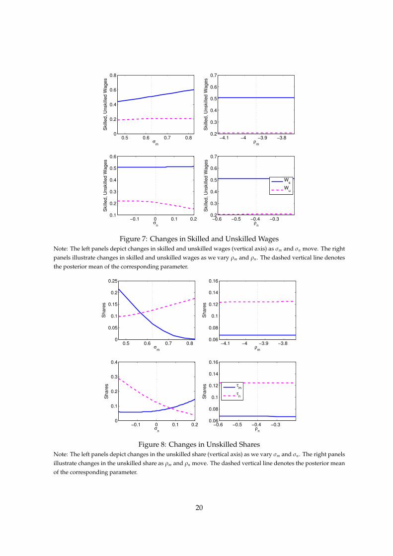
Figure 7: Changes in Skilled and Unskilled WagesNote: The left panels depict changes in skilled and unskilled wages (vertical axis) as σm and σn move. The rightpanels illustrate changes in skilled and unskilled wages as we vary ρm and ρn. The dashed vertical line denotesthe posterior mean of the corresponding parameter.
0.5 0.6 0.7 0.80
0.05
0.1
0.15
0.2
0.25
Sh
are
s
σm
−4.1 −4 −3.9 −3.80.06
0.08
0.1
0.12
0.14
0.16
Sh
are
s
ρm
−0.1 0 0.1 0.20
0.1
0.2
0.3
0.4
Sh
are
s
σn
−0.6 −0.5 −0.4 −0.30.06
0.08
0.1
0.12
0.14
0.16
Sh
are
s
ρn
τm
τn
Figure 8: Changes in Unskilled SharesNote: The left panels depict changes in the unskilled share (vertical axis) as we vary σm and σn. The right panelsillustrate changes in the unskilled share as ρm and ρn move. The dashed vertical line denotes the posterior meanof the corresponding parameter.
20
decreases.Figure 8 reveals why a reduction in σn leads to a decline in the non-manufacturing wage,
while manufacturing wage slightly increases. The reduction of capital-skill complementaritythrough σn is associated with a large increase in the share of unskilled labor in the non-manufacturing sector. To elaborate on the importance of this factor, let us express changes inthe sectoral wage (15) as
dw j = (1 − τ j)dws + τ jdwu + (wu − ws)dτ j
= dws − τ j(dws − dwu) + (wu − ws)dτ j (24)
for j = m,n. The second term in (24) represents changes in the skill premium, which arenegative in the data. Thus, the contribution of changes in the skill premium becomes positive.Given the positive skill premium, the last term (changes in the unskilled labor share, dτ j)has a negative impact on sectoral wages. While the reduced capital-skill complementarity innon-manufacturing barely changes the unskilled share in manufacturing, it sharply increasesthe unskilled share in non-manufacturing. The contribution of the increased unskilled sharein non-manufacturing dominates the positive effect that stems from the lower skill premium.As a result, the non-manufacturing wage declines. In contrast, the manufacturing wage doesnot change much due to the very small share of unskilled labor in manufacturing.
In terms of unskilled share, the opposite happens when σm decreases. The unskilledshare in manufacturing rises and that in non-manufacturing declines slightly. The rise in theunskilled share and the reduction in the skilled wage together dampen the manufacturingwage. The drop in the skilled wage dominates other factors in non-manufacturing. As aresult, declines in the non-manufacturing wage are slower than those in the manufacturingwage. Increases in ρ’s barely affect the unskilled share in either manufacturing or non-manufacturing. Given the relatively small reduction in the skilled wage, the positive effectfrom changes in the skill premium dictates sectoral wages. As a result, we see both sectoralwages rise as ρ increases.
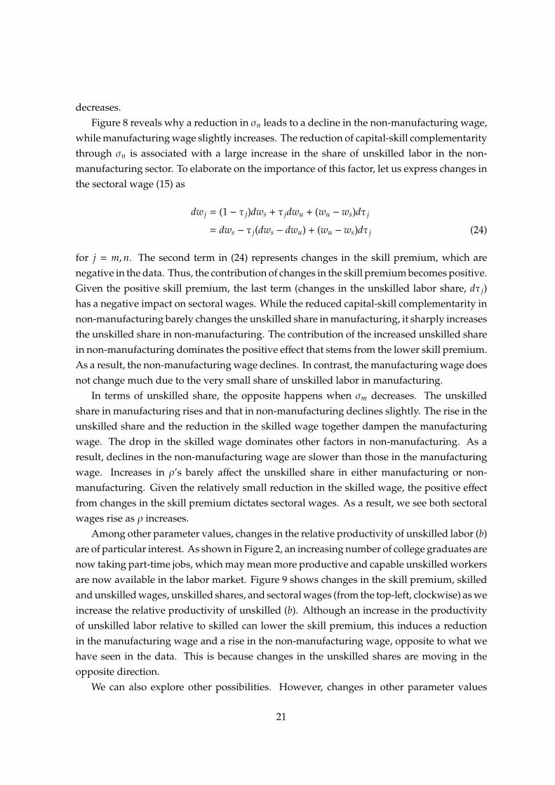
Among other parameter values, changes in the relative productivity of unskilled labor (b)are of particular interest. As shown in Figure 2, an increasing number of college graduates arenow taking part-time jobs, which may mean more productive and capable unskilled workersare now available in the labor market. Figure 9 shows changes in the skill premium, skilledand unskilled wages, unskilled shares, and sectoral wages (from the top-left, clockwise) as weincrease the relative productivity of unskilled (b). Although an increase in the productivityof unskilled labor relative to skilled can lower the skill premium, this induces a reductionin the manufacturing wage and a rise in the non-manufacturing wage, opposite to what wehave seen in the data. This is because changes in the unskilled shares are moving in theopposite direction.
We can also explore other possibilities. However, changes in other parameter values
21
0.1 0.2 0.3 0.4 0.52
2.2
2.4
2.6
2.8
ws/w
u
b0.1 0.2 0.3 0.4 0.5
0.1
0.2
0.3
0.4
0.5
0.6
Skill
ed
, U
nskill
ed
Wa
ge
s
b
Ws
Wu
0.1 0.2 0.3 0.4 0.50.45
0.5
0.55
0.6
Se
cto
ral W
ag
es
b
Wm
Wn
0.1 0.2 0.3 0.4 0.50
0.1
0.2
0.3
0.4
Sh
are
s
b
τm
τn
Figure 9: Effects of More Productive Unskilled LaborNote: The top left plot depicts changes in the skill premium as b changes. The top right panel illustrates changesin the sectoral wages and the bottom left panel shows changes in skilled and unskilled wages as b varies. Thebottom right graph shows the share of unskilled labor as a function of b. The dashed vertical line denotes thebenchmark case.
do not alter the steady-state values, especially for the skill premium and sectoral wages, ina way that is consistent with the data. Changes in other parameter values can result in areduction of the skill premium. For example, a drop in the weight for manufacturing goods(γ) lowers the skill premium. Also, an increase in the elasticity of substitution betweenskilled and unskilled labor supply (θ) reduces the skill premium. However, it turns out thatthese changes move the sectoral wages in the same direction and thus cannot account for theobserved changes in sectoral wages in the data. This is primarily because these parameterchanges do not generate meaningful changes in the unskilled shares.
To sum up, a reduction in σn (lower capital-skill complementarity in non-manufacturing)is the most likely single parameter change that can consistently explain the stylized factsoutlined in Section 2, among the numerous possibilities we have considered. That is, whilethe manufacturing wage increases slightly, the non-manufacturing wage drops, and the skillpremium declines. The value of σn that is consistent with the lower skill premium in therecent time periods, 2.3, is σn = −0.14.
5.2 Discussion
It is then natural to ask what specific change(s) in Japanese economy might explain theobserved changes illustrated in Section 2. Even though our analysis above suggests that
22

Table 4: Actual Changes and Simulation Results
Data Case 1 Case 2 Case 3 Case 4Percentage Changes in the Targets
Skill Premium (Ws/Wu) −8.61 −7.96 2.33 −11.44 −1.99Sectoral Wage Gap (Wm/Wn) 14.74 6.03 −2.89 5.90 10.36
Manufacturing Unskilled Share (τm) 1.85 1.82 4.30 1.05 −0.33Non-manufacturing Unskilled Share (τn) 9.17 11.53 −0.41 11.15 14.72Changes in Parameter Values
σn n.a. −0.19 0 −0.19 −0.19θ n.a. −0.20 −0.20 0 −0.20b n.a. 0.05 0.05 0.05 0
Note: Observed changes in the targets are measured from 1995 to 2013. We evaluate the closeness betweenthe data and the implied steady-state values by the sum of squared distances.
lower capital-skill complementarity in non-manufacturing is the main driving force behindthe changes seen since the mid-1990s, it is important to assess the qualitative contributionsof other factors. To this end, we will evaluate the impact of two other changes we haveobserved since the mid-1990s.
One is that working mothers with part-time jobs have increased markedly since the mid-1990s. In the context of our model, this is reflected as a reduction in θ, which means lesssubstitutability between part-time and full-time worker supply. It used to be the case thatmost female workers in Japan would exit the labor force upon marriage or having children.However, there is now an increasing tendency to remain in the labor force with part-timejobs. Part-time jobs may be preferred to full-time jobs given that they offer a more flexiblework schedule. As a result, working mothers would react less to changes in relative wagesacross the two types of jobs.
Another factor is an increase in the productivity of unskilled workers (i.e., an increase inb). This trend is evident from the fact that there is an increasing number of college graduatesworking in part-time (or non-regular) jobs as shown in Figure 2.
Table 4 summarizes the observed changes in the data and our simulation results. Inparticular, we pick parameter values such that percentage changes in the implied steady-state skill premium, sectoral wage gap, and unskilled shares in manufacturing and non-manufacturing become closer to those observed in reality. Case 1 corresponds to our preferredspecification. Overall performance is quite good. It seems that there is a tradeoff betweenhitting the sectoral wage gap and the manufacturing unskilled share. The results reported forCases 2 to 4, where changes in parameter value are muted one by one, tell us the quantitativeimportance of each parameter when others are held steady.
As demonstrated in Section 5.1, a reduction in σn plays a crucial role in explaining theobserved changes in the data. As evident in Case 2, if σn is not lowered, the skill premium,
23

Table 5: Changes in Non-manufacturing Industries (percentage points)
High Group Middle Group Low GroupChanges in Employment Share from 1997 to 2012 6.1 −0.0 −6.1Changes in Part-time Ratio from 1997 to 2012 5.1 4.0 2.4
Note: We classify non-manufacturing industries into three groups (high, middle, and low) by part-time ratio(ratio of part-time to total workers) in 2012. The high group includes retail trade, accommodations, eatingand drinking services, living-related and personal services, and social insurance and social welfare. The lowgroup includes electricity, gas, heat supply and water, information and communications, transport and postalactivities, wholesale trade, finance and insurance, and education, learning support. The middle group consistsof all other non-manufacturing industries. The employment share for each group is the number of workersin the group divided by total workers. Data in this table are taken from the Statistics Bureau’s EmploymentStatus Survey.
sectoral wage gap, and unskilled share in non-manufacturing move in the opposite direction.As equation (24) indicates, rapid growth in part-time non-manufacturing jobs (i.e., an increasein the unskilled share denoted by τn) is the key to a consistent interpretation. As noted inSection 2, the skill premium in Japan declined by 8.6 percent from 1995 to 2013 while thesectoral wage gap (Wm/Wn) widened over the same period.
We can see the role of lower θ from Case 3 reported in Table 4. Less substitutabilitybetween skilled and unskilled jobs helps to account for the increase in the unskilled sharein manufacturing. Similarly, the rise in b (productivity of unskilled relative to skilled) playsa role in increasing the unskilled share in manufacturing. While lower θ increases the skillpremium, higher b yields a lower skill premium.
What does the lower σn mean in the real world? A closer look at the expansion ofJapan’s service sector provides a clue as to how one might interpret lower capital-skillcomplementarity in the non-manufacturing sector. Table 5 compares changes in employmentshares and part-time ratios within non-manufacturing industries, indicating that the fastestgrowing service industries tend to be more dependent on part-time workers. Prime examplesinclude social welfare and nursing, the restaurant business, and retail, all of which are highlylabor intensive and relatively low paid jobs. Conversely, full-time-worker dependent serviceindustries tend to grow more slowly, which can result in lower σn. Even though it is noteasy to identify factors affecting the employment share of each industry within the currentframework, we can make a case that employment shares within the non-manufacturing sectorhave notably changed as a consequence of uneven growth speeds, with the resulting sectorallabor reallocation reflected in the change in the parameter value (σn) that characterizes theproduction technology of the non-manufacturing sector as a whole.
Table 5 also shows a faster increase in the part-time ratio for part-time-worker depen-dent industries, suggesting that the non-manufacturing sector as a whole turns to be moreunskilled-labor-intensive. This may reflect their efforts to minimize labor costs since themid-1990s. Moreover, these industries might prefer to employ part-time workers because
24
they are more flexible than full-time workers in terms of working hours. For example, in re-cent years, more restaurants and supermarkets have extended opening hours until midnightby utilizing part-time workers at night. Declines in σn might also reflect this change. Onthe flipside, with less capital-intensive technology, capital-skill complementarity can lose itsimportance. This interpretation suggests that the entire non-manufacturing sector has, overtime, applied a less capital-skill complementary technology on average.
Although the current paper has paid particular attention to the declining skill premiumin Japan, one implication from this study is that lower capital-skill complementarity in othercountries may be able to explain declines in their skill premiums. There are several possibleexplanations for the reduction in the skill premium. However, the role played by lowercapital-skill complementarity becomes more important and relevant if a global factor, suchas the cheaper relative price of capital goods interacting with lower trade costs, is operatingand positively affecting the skill premium, as discussed in Parro (2013). However, thishypothesis is left as an important question for future research.
6 Conclusion
While many studies document and offer explanations for rises in the skill premium acrosseconomies, less attention has been paid to declines in the skill premium observed in somecountries over the past few decades. This paper documents changes in the Japanese la-bor market at both aggregate and industry levels. We observe a decline in the skill pre-mium, a widening of the sectoral wage gap, and an increase in the unskilled share in non-manufacturing.
In order to provide a consistent explanation for the above-mentioned changes, we builda two-sector neoclassical general equilibrium model with two types of labor (skilled andunskilled), in which production technology features capital-skill complementarity. The twosectors can differ in terms of the degree of capital-skill complementarity. We use Bayesianmethods to fit our model to the Japanese data. We find evidence of sectoral heterogeneityin capital-skill complementarity. Based on the estimated structural parameters, we showthat the decline in capital-skill complementarity — reflecting the decline in the elasticity ofsubstitution between capital and unskilled labor in non-manufacturing — can account forthe observed changes in the Japanese data.
25

References
Acemoglu, D. (2002): “Technical Change, Inequality, and the Labor Market,” Journal ofEconomic Literature, 40, 7–72.
Balleer, A. and T. van Rens (2013): “Skill-biased Technological Change and the BusinessCycle,” Review of Economics and Statistics, 95, 1222–1237.
Geweke, J. (1999): “Using Simulation Methods for Bayesian Econometric Models: Inference,Development, and Communication,” Econometric Reviews, 18, 1–73.
Griliches, Z. (1969): “Capital-Skill Complementarity,” Review of Economics and Statistics, 51,465–468.
Horvath, M. (2000): “Sectoral shocks and aggregate fluctuations,” Journal of Monetary Eco-nomics, 45, 69 – 106.
Iacoviello, M., F. Schiantarelli, and S. Schuh (2011): “Input and Output Inventories inGeneral Equilibrium,” International Economic Review, 52, 1179–1213.
Kawaguchi, D. and Y. Mori (2014): “Winning the Race against Technology,” Discussionpapers 14017, Research Institute of Economy, Trade and Industry (RIETI).
Kondo, A. and S. Naganuma (2014): “Inter-industry Labor Reallocation and Task Distance,”Working paper series 14-e-8, Bank of Japan.
Krusell, P., L. E. Ohanian, J.-V. Rıos-Rull, and G. L. Violante (2000): “Capital-skill Com-plementarity and Inequality: A Macroeconomic Analysis,” Econometrica, 68, 1029–1053.
Lindquist, M. J. (2004): “Capital–skill Complementarity and Inequality Over the BusinessCycle,” Review of Economic Dynamics, 7, 519–540.
Maliar, L. and S. Maliar (2011): “Capital–Skill Complementarity and Balanced Growth,”Economica, 78, 240–259.
Marquis, M. and B. Trehan (2010): “Relative productivity growth and the secular “decline”of U.S. manufacturing,” The Quarterly Review of Economics and Finance, 50, 67–74.
Ngai, L. R. and C. A. Pissarides (2007): “Structural Change in a Multisector Model ofGrowth,” American Economic Review, 97, 429–443.
Parro, F. (2013): “Capital-Skill Complementarity and the Skill Premium in a QuantitativeModel of Trade,” American Economic Journal: Macroeconomics, 5, 72–117.
Polgreen, L. and P. Silos (2008): “Capital–skill Complementarity and Inequality: A Sensi-tivity Analysis,” Review of Economic Dynamics, 11, 302–313.
26

Sugo, T. and K. Ueda (2008): “Estimating a Dynamic Stochastic General Equilibrium Modelfor Japan,” Journal of the Japanese and International Economies, 22, 476–502.
27

Appendix
A Steady-State Relationship
To simplify the presentation below, let us define for j = m,n in the steady state
Z j ≡ µ j
(ψuU j
ψsS j
)σ j
+ (1 − µ j){λ j
(K j
ψsS j
)ρ j
+ (1 − λ j)} σ jρ j
. (25)
Given the steady-state value of r = 1β − (1 − δ) and other parameter values, together with the
definitions of Zm and Zn in (25), the following non-linear system of 12 equations characterizesthe steady state of this economy.
Ym
ψsSm= Am(Zm)
1σm
Yn
ψsSn= An(Zn)
1σn
Cm
ψsSm=
Ym
ψsSm− δ
Km
ψsSm− δ
Kn
ψsSn
Sn
Sm
Cn
ψsSn=
Yn
ψsSn
p(
Cn
ψsSn
) 1κ
=(1 − γ)γ
(Cm
ψsSm
Sm
Sn
) 1κ
( ws
wu
)θ=
Sm
Um
(1 + Sn
Sm
)(1 + Un/Sn
Um/Sm
SnSm
)r = (1 − µm)λmAm
(Km
ψsSm
)ρm−1
(Zm)1−σmσm
{λm
(Km
ψsSm
)ρm
+ (1 − λm)} σm−ρm
ρm
rp
= (1 − µn)λnAn
(Kn
ψsSn
)ρn−1
(Zn)1−σnσn
{λn
(Kn
ψsSn
)ρn
+ (1 − λn)} σn−ρn
ρn
ws = (1 − µm)(1 − λm)(Am)σm
(Ym
ψsSm
)1−σm {λm
(Km
ψsSm
)ρm
+ (1 − λm)} σm−ρm
ρm
ws
p= (1 − µn)(1 − λn)(An)σn
(Yn
ψsSn
)1−σn {λn
(Kn
ψsSn
)ρn
+ (1 − λn)} σn−ρn
ρn
wu = µm(Am)σm
(Ym
ψsSm
)1−σm (ψuUm
ψsSm
)σm−1
ψu
wu
p= µn(An)σn
(Yn
ψsSn
)1−σn (ψuUn
ψsSn
)σn−1
ψu
28

This system describes the steady-state relationship among the following 12 variables:
Ym
Sm,
Yn
Sn,
Cm
Sm,
Cn
Sn,
Km
Sm,
Kn
Sn,
Um
Sm,
Un
Sn,
Sn
Sm, p,ws,wu.
B Log-Linearized System
The log-linearized system of equations used in the estimation in Section 4 is as follows.
ct = ωmcm,t + (1 − ωm)cn,t
Λt = −1κ
cm,t +(1κ− 1
)ct
Λt + pt = −1κ
cn,t +(1κ− 1
)ct
ht = ωsst + (1 − ωs)ut
Λt + ws,t =1θ
st +
(1η−
1θ
)ht + ms,t
Λt + wu,t =1θ
ut +
(1η−
1θ
)ht + mu,t
Λt = Ψm,t + ξm,t + ϕ{im,t−1 − (1 + β)im,t + βEt[im,t+1]
}Λt = Ψn,t + ξn,t + ϕ
{in,t−1 − (1 + β)in,t + βEt[in,t+1]
}Ψm,t = βEt
[rΛt+1 + rrm,t+1 + (1 − δ)Ψm,t+1
]Ψn,t = βEt
[rΛt+1 + rrn,t+1 + (1 − δ)Ψn,t+1
]xm,t = (σm − ρm)
{ωkm km,t + (1 − ωkm)(ψs,t + sm,t)
}xn,t = (σn − ρn)
{ωkn kn,t + (1 − ωkn)(ψs,t + sn,t)
}rm,t = (1 − σm)ym,t + σmam,t + (ρm − 1)km,t + xm,t
rn,t − pt = (1 − σn)yn,t + σnan,t + (ρn − 1)kn,t + xn,t
ws,t = (1 − σm)ym,t + σmam,t + ρmψs,t + (ρm − 1)sm,t + xm,t
ws,t − pt = (1 − σn)yn,t + σnan,t + ρnψs,t + (ρn − 1)sn,t + xn,t
wu,t = (1 − σm)ym,t + σmam,t + σmψu,t + (σm − 1)um,t
wu,t − pt = (1 − σn)yn,t + σnan,t + σnψu,t + (σn − 1)un,t
ym,t = am,t + ωum(um,t + ψu,t) + (1 − ωum)xm,t
yn,t = an,t + ωun(un,t + ψu,t) + (1 − ωun)xn,t
km,t+1 = δim,t + (1 − δ)km,t
kn,t+1 = δin,t + (1 − δ)kn,t
29

st = fssm,t + (1 − fs)sn,t
ut = fuum,t + (1 − fu)un,t
ym,t = ωccm,t + ωi im,t + (1 − ωc − ωi)in,t
yn,t = cn,t
am,t = ρal am,t−1 + εam,t
an,t = ρan an,t−1 + εan,t
ψs,t = ρψsψs,t−1 + εψs,t
ψu,t = ρψuψu,t−1 + εψu,t
ξl,t = ρξl ξl,t−1 + εξl,t
ξn,t = ρξn ξn,t−1 + εξn,t
ms,t = ρmsms,t−1 + εms,t
mu,t = ρmumu,t−1 + εmu,t
wm,t = ηχmχm,t + ηwsmws,t + ηwu,1wu,t
wn,t = ηχnχn,t + ηwsnws,t + ηwu,2wu,t
χm,t = ηum um,t + ηsm sm,t
χn,t = ηun un,t + ηsn sn,t
where
ωm =γ(Cm)
κ−1κ
γ(Cm)κ−1κ + (1 − γ)(Cn)
κ−1κ
=Cm
Cm + pCnωs =
(S)θ+1θ
(S)θ+1θ + (U)
θ+1θ
ϕ = Φ′′(1)
ωkm =λm(Km)ρm
λm(Km)ρm + (1 − λm)(ψsSm)ρmωkn =
λn(Kn)ρn
λn(Kn)ρn + (1 − λn)(ψsSn)ρn
ωum =µm(ψuUm)σm
µm(ψuUm)σm + (1 − µm)(Xm)σm
(σm−ρm)ωun =
µn(ψuUn)σn
µn(ψuUn)σn + (1 − µn)(Xn)σn
(σn−ρn)
fs =Sm
Sfu =
Um
U
ωc =Cm
Ymωi =
Im
Ym
ηχm =1 − π
SmUmπ + 1
ηχn =1 − π
SnUnπ + 1
ηwsm=
1 +1
SmUmπ
−1
ηwsn=
1 +1
SnUnπ
−1
ηwum=
(1 +
Sm
Umπ)−1
ηwun=
(1 +
Sn
Unπ)−1
30

C Data Construction
Since there are no quarterly output and price data at the sectoral level, we assume thatsemi-durable and durable goods, and investment goods for residential and business fixedinvestment are produced by the manufacturing industry (Ym). Also, we assume that non-durable goods and services are produced by the non-manufacturing industry (Yn). Weconstruct price indices for each output accordingly (Pm and Pn). The relative price (p) isdefined as Pn/Pm. We obtain GDP components and corresponding price indices from theCabinet Office’s National Accounts.
Population (15 years old and over) consists of labor force and non-labor force (excludingpeople with unknown labor status), which are taken from the Labour Force Survey (LFS) bythe Statistics Bureau of the Ministry of Internal Affairs and Communications. This is used toconvert quantity variables in per capita term.
We construct the sectoral hourly wage (Wm and Wn) by dividing the nominal wage billper worker by total hours worked per worker for each industry. Until 1989, we use datafrom establishments with 30 or more employees. From 1990 onwards, we use data fromestablishments with 5 or more employees. These data are taken from the Monthly LabourSurvey (MLS) by the Ministry of Health, Labour and Wealth.
Part-time workers are defined as those who work fewer hours than regular (full-time)workers per day or per week. From 1990, we use the numbers of full-time (Ls) and part-time(Lu) workers reported in the MLS. However, there are no official statistics until 1989. Weextrapolate the number reported in the MLS by using the data from the LFS. We categorizeemployees who work at least 35 hours per week as full-time workers and those workingshorter hours as part-time workers.
We construct the average hours worked per full-time worker by using the followingrelationship:
h =hsLs + huLu
Ls + Lu= hs
( Ls
Ls + Lu+ ζ
Lu
Ls + Lu
),
where h is the average hours worked per worker, hs and hu are the average hours workedper full-time and per part-time worker, Ls and Lu denote the numbers of full-time and part-time workers, and ζ = hu
hs. To measure h, we use the MLS. From 1990, we use data from
establishments with five or more employees. Until 1989, we use data from establishmentswith 30 or more employees. ζ is taken from the MLS from 1990 (establishments with five ormore employees). Until 1989, we use the Basic Survey on Wage Structure by utilizing linearinterpolation. Given h, Ls, Lu, and ζ, we construct hs and then calculate hu = ζhs. Finally, weconstruct by S = hsLs and U = huLu.
31