rice producers’ behavior towards unpredictable price … valley, ilocos region, western visayas...

International Journal of Development and Sustainability

ISSN: 2168-8662 – www.isdsnet.com/ijds

Volume 3 Number 1 (2014): Pages 1-19

ISDS Article ID: IJDS13111901

Rice producers’ behavior towards unpredictable price and ambient temperature changes: Analysis with ARCH and SUR for the major agricultural regions in the Philippines

Raquel M. Balanay 1*, Harold Glenn A. Valera 2 1 Caraga State University, Ampayon, Butuan City, Philippines 8600 2 International Rice Research Institute, DAPO Box 7777, Metro Manila, Philippines

Abstract

The study has investigated the behavior of rice prices and mean temperature levels in Central Luzon, CALABARZON,

Cagayan Valley, Ilocos Region, Western Visayas and Northern Mindanao, which are the major rice producing areas in

the Philippines. ARCH is used to analyze the changes of these variables to determine whether these changes can pose

risks through their volatilities to the rice producers. SUR is used to determine through supply response estimations

the influence of which on rice production in the said areas of the country. Results of the study indicate that rice

prices and mean temperature levels in the concerned areas have volatile changes, which can augment the risks faced

by rice producers in the country. But the volatile changes and risks posed by these variables are found not to affect

rice production in the said areas. This finding may be attributed to the programs of the Philippine government for

the improvement of the rice industry for increased efficiency. Sustained efforts of the government and other entities

for the development of rice industry in the country may enable it to gain competitiveness particularly in the global

market.

Keywords: ARC; SUR; volatility; supply response and risks

* Corresponding author. E-mail address: [email protected]

Submitted: 19 November 2013 Accepted: 23 December 2013 Published: 10 January 2014

Published by ISDS LLC, Japan Copyright © 2014 by the Author(s) This is an open access article distributed under the

Creative Commons Attribution License, which permits unrestricted use, distribution, and reproduction in any medium,

provided the original work is properly cited.

Cite this article as: Balanay, R.M. and Valera, H.G.A. (2014), “Rice producers’ behavior towards unpredictable price and

ambient temperature changes: Analysis with ARCH and SUR for the major agricultural regions in the Philippines”,

International Journal of Development and Sustainability, Vol. 3 No. 1, pp. 1-19.

International Journal of Development and Sustainability Vol.3 No.1 (2014): 1-19

2 ISDS www.isdsnet.com

1. Introduction

Rice is a staple commodity and a pivotal political commodity since the Commonwealth period in the

Philippines (Intal and Garcia, 2005). The Asian Development Bank (ADB) has quoted it as a critical item since

it constitutes 34% of the food expenditure of the bottom 20% of households in the country. Daily, rice is

consumed in quantities reported to be more than 30 thousand metric tons. An increase in the price of rice is

said to result to workers demanding wage increases throughout the nation. Essentially, this has merited the

importance of stabilizing rice market conditions, particularly its prices, supply and demand to avoid

unfavorable disruptions, comprising of street protests that could affect the conduct of business in the major

commercial districts of the Philippines (Senate Economic Planning Office, 2010).

However, volatile conditions could not warrant the certainty of insulating rice markets in the Philippines

by merely increasing production to remain stable. Commodity prices fluctuate naturally and weather

conditions are beyond human control, thus, rice markets have to deal with volatile elements as efficiently as

possible. Particularly, fluctuating prices are considered crucial in market analysis because they affect the

decisions made by producers and consumers (Bernard et al., 2006). Price volatility translates to significant

price risks that complicate established agribusiness practices (Rezitis and Stavropoulos, 2009 and Mark et al.,

2008 as cited by Karali and Power, 2009). Nam Tran et al. (2012) has reported price volatility and increased

variability in crop yields as among the effects to watch out under climate variability, which can be

detrimental to market welfare since volatile consequences could disrupt commodity markets on a

considerable scale by confounding the bases for decision-making (Spargoli and Zagaglia, 2007; Kargbo, 2009;

Du et al., 2009).

In this study, the prices of rice are evaluated to detect the presence of volatile behavior through an

autoregressive conditionally heteroscedastic approach (ARCH). ARCH is originally a popular technique for

monitoring the volatilities of financial variables for highly speculative transactions in financial markets, but it

has found its way into agricultural market analysis in recent years for cases involving risk estimations in time

series. Similar approach has been applied as well in determining the behavior of ambient temperature

changes over time, because it can generate values of expected variance (volatility estimates) that could be

analyzed later with the response of rice production in the country. The use of the said approach for this study

has been based on the research works of Rezitis and Stavropoulos (2009) and Jordaan et al. (2007), which

had estimated the pattern of fluctuations in agricultural markets and had analyzed the responses of

agricultural markets to such pattern for policy actions.

The same framework is used in this study, but the analysis has been extended to cover the effects of

temperature changes as basis for climate-change-related policies. The inclusion of ambient temperature in

the study may serve as a proxy variable to the effect of climate change in rice production. Its incorporation in

the supply response model for rice could tell the producers’ general response to its changes, which is vital in

defining the courses of action for increased resilience and adaptation to climate change among the rice

producers in the country. Nam Tran et al. (2012) has recently formulated a model that has combined the

estimation of the effects of price volatility and climate change to production, which could estimate losses

through simulations when volatility in prices and climate change are heightened. The interest of this study is


ISDS www.isdsnet.com 3

on producer’s response when risks due to the changing prices and temperature are being confronted. Thus,

this research focuses on analyzing the behavior of the rice producers towards changes in temperature and

prices in the major agricultural areas in the Philippines to determine the policies relevant to building the

resilience and efficiency of the rice industry in the country, besides sustaining efforts towards global

competitiveness.

2. Review of related literature

Interests on volatile factors are given by the fact that it can influence subsequent actions and that agricultural

economists have started to notice the importance of investigating risk aversion in commodity markets

(Rezitis and Stavropoulos, 2009).The literatures related to the said topic have been reviewed herein. The

analysis of Oktaviani et al. (2011) has produced results that have inferences on rice production in Indonesia.

IMPACT model has been used in the analysis, which is a partial equilibrium model of the agricultural sector,

representing a competitive agricultural market for crops and livestock. The model has shown that with food

price shocks, negative impacts from climate change would heighten. Climate change scenario formulation is

carried out in technical simulations utilizing the global circulation model (GCM) datasets, consisting of

precipitation, maximum daily temperature and minimum air temperature. The inclusion of temperature data

in the model is due to the fact that these data are sufficiently and publicly available.

The monitoring and utilization of temperature in productivity studies has been also noted in the case of

managing and sharing the risk of drought in Australia. Hertzler et al. (2006, p. 5) have reported that “most

climate models forecast warmer conditions across Australia with the implication that dairy and beef cattle

will experience even greater heat stress, causing greater mortality and limitations on productivity.”Their

report has also pointed out that agricultural decision-making in the same country is done under a situation of

high uncertainty because of risks associated with increased temperature. Since farm resources are usually

allocated and determined prior to having known yields and product prices, farmers have to allocate these

resources every season based on their expectations on yields and prices (Anderson, 2003 as cited by Hertzler,

Kingwell, Crean and Carter, 2006). As such, the accuracy of forming expectations has bearing on how the said

resources would be used efficiently, which has repercussions on the amount of farm income to be generated

(Hertzler et al., 2006).

Studies using temperature changes in relation to agricultural productivity have been increasing through

the years due to the impacts of climate change and these can be found in the works of Thurlow et al. (2011),

Dono et al. (2012), Cunha et al. (2012), Ringler et al. (2010), Hertel and Rosch (2010) and Deressa (2008) for

the recent period, where the analysis through temperature changes are intertwined with the concept of

evapotranspiration. FAO (2013) has stated that “evapotranspiration (ET) is a concept that refers to the

combination of evaporation and transpiration processes whereby water is lost on the one hand from the soil

surface by evaporation and on the other hand from the crop by transpiration.” Air temperature is among the

principal weather parameters that affect evapotranspiration, according to FAO (2013). Thus, in this study,

the volatility of ambient temperature would have to be understood as referring to the degree at which



changes of temperature can become difficult to predict. As stated in the report of Krechowicz et al. (2010),

the most financially material impacts of climate change and water scarcity are increased agricultural input

prices and increased processing costs. Food commodity prices are particularly sensitive to the shocks

induced by unpredictable extreme weather conditions, while animal yields are put at risk when water

temperature is increased and access to clean water supplies becomes limited, according to Krechowicz et al.

(2010).

On the other hand, studies on price volatility have likewise spiraled, because of the importance of forming

price expectations in agricultural commodity markets (Rezitis and Stavropoulos, 2009). The ability to

forecast accurately the prices of commodities greatly matters in policy and business circles (Bernard et al.,

2006). Volatile movements in prices are associated with risks and uncertainties (Rezitis and Stavropoulos,

2009; Jordaan et al., 2007 and Rezitis, 2003 as cited by Balanay, 2011). As reported by Kargbo (2005), highly

volatile prices are a deterrent to agricultural productivity, which tend to intensify inflationary pressures.

Such prices can increase the uncertainty faced by farmers and agribusiness firms, which affect farmer’s

investment decisions and have serious ramifications on the growing farm debt, decreasing farm income and

productivity. Volatile movements have been captured for analysis in several models in several studies

already. Examples of which is the use of threshold autoregressive (TAR) models in the study of Ramirez

(2009) where the model specification has allowed two different autocorrelation regimes depending on the

value of the error terms; partial equilibrium and time series WEMAC 2.0 model in the study of Benjamin et al.

(2009), and stochastic volatility models and Bayesian Markov Chain Monte Carlo methods in the study of Du

et al. (2009).

However, for researches which deal with expectations in the empirical analysis of risks in commodity

markets, autoregressive conditionally heteroscedastic (ARCH) has been preferred as in the studies of

Aradhyula and Holt (as cited by Rezitis and Stavropoulos, 2009), Rezitis (2003), Rezitis and Stavropoulos

(2009) and Bekkerman and Pelletier (2009). These studies have generated the evidence of price volatility as

an important risk factor in supply response functions. Particularly, ARCH or generalized ARCH (GARCH) is

used to estimate price uncertainty in the Greek broiler market, and quadratic NAGARCH model to capture

better the producer’s price volatility in the Greek pork sector in the study of Rezitis and Stavropoulos (2009).

In view of the aforementioned studies, this research is founded on the estimation procedures and analytical

procedures used by Rezitis and Stavropoulos (2009) with double expected variances (volatilities of prices

and temperature levels) to determine the behavior of rice producers toward the changes in rice prices and

temperature levels in the major rice-producing areas of the Philippines.

3. Data and model specification

The data used in this study are comprised of the monthly retail prices of rice, quarterly supply of rice in the

major rice-producing regions or areas in the Philippines, monthly retail prices of corn and climate data

consisting of monthly mean temperature and rainfall amount in similar areas. The time period covered in

these data is 1994 to 2011. The major rice-producing regions or areas are identified from the supply data by



region. Except for the climate data, all these data are taken from the Bureau of Agricultural Statistics (BAS) of

the Department of Agriculture (DA) through its online information service at Countrystat website. The data

on mean temperature and rainfall amount are obtained from the Philippine Atmospheric, Geophysical and

Astronomical Services Administration (PAGASA) of the Department of Science and Technology (DOST).

However, for the price data, monthly consumer price indices (CPI) have been used to deflate these prices

before using them in the analysis. These CPI values are taken from the online information facility of the

National Statistical Coordination Board (NSCB). The major rice-producing areas of the Philippines whose

supply responses are analyzed in this study are Central Luzon, CALABARZON, Cagayan Valley, Ilocos Region,

Western Visayas and Northern Mindanao (BAS, 2012).

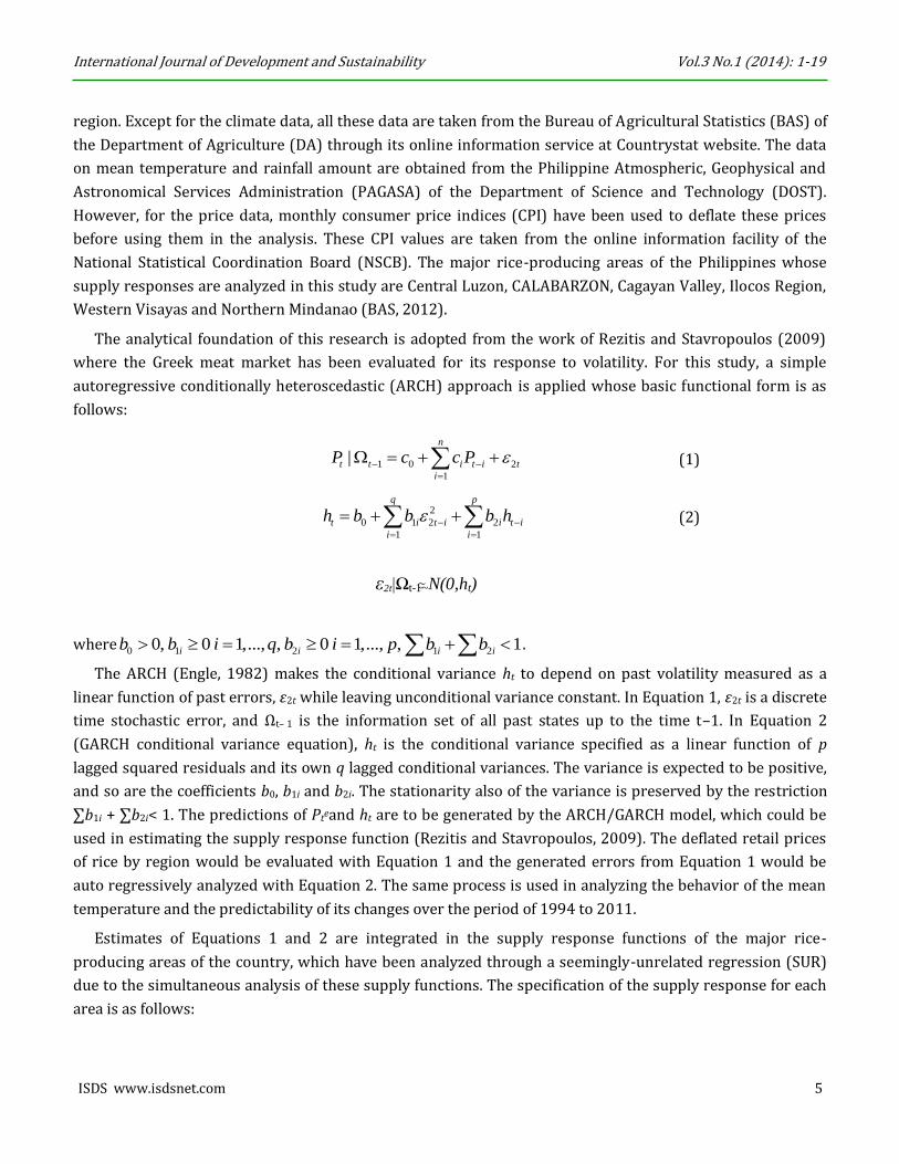
The analytical foundation of this research is adopted from the work of Rezitis and Stavropoulos (2009)

where the Greek meat market has been evaluated for its response to volatility. For this study, a simple

autoregressive conditionally heteroscedastic (ARCH) approach is applied whose basic functional form is as

follows:

1 0 2

1

|n

t t i t i t

i

P c c P

(1)

(2)

ε2t|Ωt-1 ~N(0,ht)

where0 1 2 1 20, 0 1,..., , 0 1,..., , 1i i i ib b i q b i p b b .

The ARCH (Engle, 1982) makes the conditional variance ht to depend on past volatility measured as a

linear function of past errors, ε2t while leaving unconditional variance constant. In Equation 1, ε2t is a discrete

time stochastic error, and Ωt– 1 is the information set of all past states up to the time t–1. In Equation 2

(GARCH conditional variance equation), ht is the conditional variance specified as a linear function of p

lagged squared residuals and its own q lagged conditional variances. The variance is expected to be positive,

and so are the coefficients b0, b1i and b2i. The stationarity also of the variance is preserved by the restriction

∑b1i + ∑b2i< 1. The predictions of Pteand ht are to be generated by the ARCH/GARCH model, which could be

used in estimating the supply response function (Rezitis and Stavropoulos, 2009). The deflated retail prices

of rice by region would be evaluated with Equation 1 and the generated errors from Equation 1 would be

auto regressively analyzed with Equation 2. The same process is used in analyzing the behavior of the mean

temperature and the predictability of its changes over the period of 1994 to 2011.

Estimates of Equations 1 and 2 are integrated in the supply response functions of the major rice-

producing areas of the country, which have been analyzed through a seemingly-unrelated regression (SUR)

due to the simultaneous analysis of these supply functions. The specification of the supply response for each

area is as follows:

2

0 1 2 2

1 1

q p

t i t i i t i

i i

h b b b h



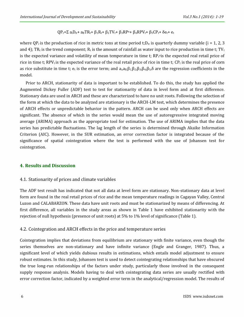
QPr=Σ aiDit+ aBTRt+ β1Rt+ β2TVt+ β3RPe+ β4RPVt+ β5CPt+ δet+ et

where QPr is the production of rice in metric tons at time period t;Dit is quarterly dummy variable (i = 1, 2, 3

and 4); TRt is the trend component; Rt is the amount of rainfall as water input to rice production in time t; TVt

is the expected variance and volatility of mean temperature in time t; RPteis the expected real retail price of

rice in time t; RPVt is the expected variance of the real retail price of rice in time t; CPt is the real price of corn

as rice substitute in time t; et is the error term; and ai,aB,β1,β2,β3,β4,β5,δ are the regression coefficients in the

model.

Prior to ARCH, stationarity of data is important to be established. To do this, the study has applied the

Augmented Dickey Fuller (ADF) test to test for stationarity of data in level form and at first difference.

Stationary data are used in ARCH and these are characterized to have no unit roots. Following the selection of

the form at which the data to be analyzed are stationary is the ARCH-LM test, which determines the presence

of ARCH effects or unpredictable behavior in the pattern. ARCH can be used only when ARCH effects are

significant. The absence of which in the series would mean the use of autoregressive integrated moving

average (ARIMA) approach as the appropriate tool for estimation. The use of ARIMA implies that the data

series has predictable fluctuations. The lag length of the series is determined through Akaike Information

Criterion (AIC). However, in the SUR estimation, an error correction factor is integrated because of the

significance of spatial cointegration where the test is performed with the use of Johansen test for

cointegration.

4. Results and Discussion

4.1. Stationarity of prices and climate variables

The ADF test result has indicated that not all data at level form are stationary. Non-stationary data at level

form are found in the real retail prices of rice and the mean temperature readings in Cagayan Valley, Central

Luzon and CALABARZON. These data have unit roots and must be stationarized by means of differencing. At

first difference, all variables in the study areas as shown in Table 1 have exhibited stationarity with the

rejection of null hypothesis (presence of unit roots) at 5% to 1% level of significance (Table 1).

4.2. Cointegration and ARCH effects in the price and temperature series

Cointegration implies that deviations from equilibrium are stationary with finite variance, even though the

series themselves are non-stationary and have infinite variance (Engle and Granger, 1987). Thus, a

significant level of which yields dubious results in estimations, which entails model adjustment to ensure

robust estimates. In this study, Johansen test is used to detect cointegrating relationships that have obscured

the true long-run relationships of the factors under study, particularly those involved in the consequent

supply response analysis. Models having to deal with cointegrating data series are usually rectified with

error correction factor, indicated by a weighted error term in the analytical/regression model. The results of



the Johansen test for cointegration are shown in Table 2, where the presence of which is noted to be

significant–thus, a model adjustment would have to incorporate an error correction factor.

In the test for ARCH effects, ARCH-LM test is used, where its results are depicted in Table 3. ARCH effects

indicate the presence of unpredictable tendencies of the data series and thus warrant the use of ARCH in the

succeeding analysis of price and mean temperature changes. The results in Table 3 show that the retail prices

of rice and mean temperature have significant ARCH effects in all major rice producing areas in the country,

namely: Central Luzon, CALABARZON, Cagayan Valley, Ilocos Region, Western Visayas and Northern

Mindanao. This means that ARCH is valid for the analysis of changes in rice prices and in mean temperature.

Table 1. Augmented Dickey Fuller Test Results for Rice Prices and Mean Temperature

ADF Test Statistics

Variable Ilocos Region Cagayan Valley Central Luzon CALABARZON Western Visayas

Northern Mindanao

L FD L FD L FD L FD L FD L FD Real retail price of rice

-2.8***

-8.0*** -2.5

-10.2*** -2.2

-11.0*** -1.9

-7.3*** -2.7** -4.1*** -2.7** -4.1***

Mean temperature

-5.4***

-8.7*** -2.5 -9.1*** -2.7

-14.9*** -2.4

-6.6*** -3.0**

-12.1*** -2.9** -6.3***

Note: *** and ** are significant at the 1% level and 5% level, respectively.

Table 2. Cointegration Test (Johansen) Results for the Commodities in the Supply Response Analysis

Commodity Region/Lag length

Hypothesized No. of CE(s)

Rice production

k = 0 k ≤ 1 k ≤ 2 k ≤ 3 k ≤ 4 k ≤ 5 k ≤ 6 k ≤ 7 k ≤ 8 Ilocos Region (3) 360.18*** 261.57*** 192.30*** 137.51*** 103.52*** 71.17*** 49.10*** 29.42*** 13.03*** Cagayan Valley (1) 523.13*** 380.12*** 271.22*** 207.20*** 152.17*** 104.04*** 61.22*** 32.17*** 11.61*** Central Luzon (1) 524.26*** 392.02*** 292.82*** 207.24*** 138.99*** 96.74*** 57.70*** 31.51*** 13.66*** CALABARZON (1) 738.04*** 484.64*** 376.42*** 285.25*** 197.91*** 136.50*** 87.26*** 50.14*** 19.82*** Western Visayas (1) 546.61*** 383.1*** 285.7*** 191.80*** 133.34*** 93.78*** 57.94*** 29.40*** 7.44*** Northern Mindanao (1) 470.52*** 372.66*** 292.74*** 219.24*** 168.42*** 124.03*** 80.86*** 46.68*** 21.30***

The Trace test was used to test the null hypothesis that the number of cointegrating vectors is less than or equal to k, where k is equal to 0 to 6.

***, ** and * indicates that the null hypothesis is rejected at the 1%, 5% and 10% levels, respectively.

The lag length chosen by the AIC criteria is shown in parentheses after relevant poultry product.



4.3. Volatility of rice prices in the major rice-producing regions in the Philippines

The analysis of the changes of rice prices intends to capture the volatile movements in the price series, which

are associated with price risks in the rice markets. Volatile price movements increase market uncertainties

because of the difficulty of forming price and/or market expectations. This is usually linked with the inability

of commodity markets to develop and compete sustainably. In the analysis of rice price volatility with ARCH,

the results are presented in two categories: expected price levels as exhibited in the results under the mean

equation and the expected price variances (ARCH/GARCH parameters) as shown under the variance

equation. The expected price levels could reveal the formation of price expectations among commodity

producers as possibly practiced when found significant in supply response analysis. The expected variances

by its significance indicate price volatility that are associated with price risks, because the range within

which price can vary is widened (Rezitis, 2003).

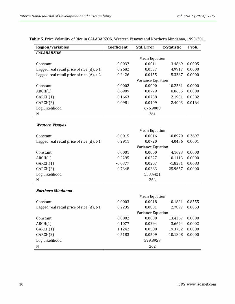
As shown in Tables 4 and 5, the results of price analysis through ARCH for Ilocos Region, Cagayan Valley,

Central Luzon, CALABARZON, Western Visayas and Northern Mindanao indicate the presence of price

volatility, wherein changes in rice prices in the said regions are expected to be unpredictable. Thus, rice

producers and consumers in the said regions are confronted with market risks, which would make them face

the difficulty of forming market expectations and decisions. The indicators of price volatility are indicated by

the highly significant coefficients of ARCH/GARCH parameters under the variance equations of Tables 4 and

5. On the other hand, the parameters under the mean equations of the same tables show the bases of forming

price expectations among the rice producers and consumers in the aforementioned regions or areas.

Table 3. ARCH-LM Test Results for ARCH Effects Among the Prices and Climate Variables by Region, 1990-2011

Variable Ilocos Region

Cagayan Valley

Central Luzon

CALABARZON Western Visayas

Northern Mindanao

F-Statistic Real retail price of rice 31.6416*** 14.4669*** 15.1307*** 40.9349*** 0.5198*** 23.3886*** Mean temperature 11.8535*** 4.1270** 3.5737** 5.6667** 1019.1760*** 12.5530***

Observed Square of Residual Real retail price of rice 28.4366*** 13.8122*** 14.4112*** 35.6563*** 0.5227 21.6296*** Mean temperature 11.4254*** 4.0939** 7.0365** 5.5888** 210.0121*** 23.1594***

Note: *** and ** are significant at the 1% level and 5% level, respectively.

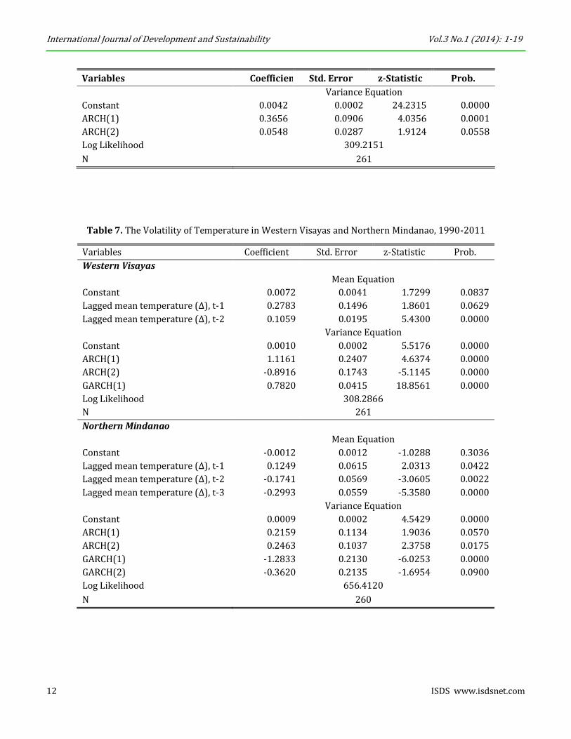
4.1. Volatility of mean temperature in the major rice-producing regions in the Philippines

Tables 6 and 7 depict the results of analyzing ambient temperature in similar regions with the use of ARCH.

These results have to be interpreted in the same way as how the earlier results in Tables 4 and 5 are

understood. Temperature changes are noted to be likewise volatile, but a bit less compared to the changes in

rice prices. This finding still implies that rice producers are confronted with risks due to changes in ambient



temperature, because warming can worsen at any point in time. In terms of expectations about the levels of

ambient temperature, most of the regions account the levels of temperature for two months, although in the

case of Cagayan Valley, the significant basis is the level of temperature in the previous four months.

Table 4. Price Volatility of Rice in Ilocos Region, Cagayan Valley and Central Luzon, 1990-2011

Region/Variables Coefficient Std. Error z-Statistic Prob.

Ilocos Region

Mean Equation

Constant -0.0028 0.0011 -2.6101 0.0091

Lagged real retail price of rice (∆), t-1 0.3180 0.0836 3.8038 0.0001

Lagged real retail price of rice (∆), t-2 -0.1347 0.0416 -3.2403 0.0012

Variance Equation

Constant 0.0000 0.0000 7.8829 0.0000

ARCH(1) 0.4041 0.0419 9.6333 0.0000

GARCH(1) 1.1206 0.0454 24.6625 0.0000

GARCH(2) -0.4323 0.0311 -13.8969 0.0000

Log Likelihood 628.3321

N 261

Cagayan Valley

Mean Equation

Constant -0.0034 0.0011 -3.0347 0.0024




Variance Equation

Constant 0.0000 0.0000 4.4405 0.0000

ARCH(1) 0.5934 0.0818 7.2533 0.0000

GARCH(2)


N 260

Central Luzon

Mean Equation

Constant -0.0021 0.0004 -4.9268 0.0000


Variance Equation

Constant 0.0001 0.0000 6.6953 0.0000

ARCH(1) 1.0901 0.1175 9.2788 0.0000


N 262



Table 5. Price Volatility of Rice in CALABARZON, Western Visayas and Northern Mindanao, 1990-2011

Region/Variables Coefficient Std. Error z-Statistic Prob.

CALABARZON

Mean Equation

Constant -0.0037 0.0011 -3.4869 0.0005



Variance Equation

Constant 0.0002 0.0000 10.2581 0.0000

ARCH(1) 0.6909 0.0779 8.8655 0.0000

GARCH(1) 0.1663 0.0758 2.1951 0.0282

GARCH(2) -0.0981 0.0409 -2.4003 0.0164


N 261

Western Visayas

Mean Equation

Constant -0.0015 0.0016 -0.8970 0.3697


Variance Equation

Constant 0.0001 0.0000 4.1693 0.0000

ARCH(1) 0.2295 0.0227 10.1113 0.0000

GARCH(1) -0.0377 0.0207 -1.8231 0.0683

GARCH(2) 0.7348 0.0283 25.9657 0.0000


N 262

Northern Mindanao

Mean Equation

Constant -0.0003 0.0018 -0.1821 0.8555


Variance Equation

Constant 0.0002 0.0000 13.4367 0.0000

ARCH(1) 0.1077 0.0294 3.6644 0.0002

GARCH(1) 1.1242 0.0580 19.3752 0.0000

GARCH(2) -0.5183 0.0509 -10.1808 0.0000


N 262



Table 6. The Volatility of Temperature in Ilocos Region, Cagayan Valley, Central Luzon and CALABARZON, 1990-2011

Variables Coefficient Std. Error z-Statistic Prob.

Ilocos Region

Mean Equation

Constant -0.0001 0.0065 -0.0171 0.9864

Lagged mean temperature (∆), t-1 -0.1588 0.0716 -2.2177 0.0266

Variance Equation

Constant 0.0078 0.0010 8.2016 0.0000

ARCH(1) 0.0972 0.0534 1.8216 0.0685

ARCH(2) -0.1150 0.0265 -4.3392 0.0000

GARCH(1) 0.5350 0.0670 7.9868 0.0000


N 262

Cagayan Valley

Mean Equation

Constant -0.0018 0.0066 -0.2713 0.7862





Variance Equation

Constant 0.0103 0.0005 20.9727 0.0000

ARCH(1) 0.1374 0.0801 1.7145 0.0864

ARCH(2) 0.0089 0.0152 0.5865 0.5575

ARCH(3) -0.0565 0.0098 -5.7453 0.0000


N 259

Central Luzon

Mean Equation

Constant -0.0107 0.0511 -0.2097 0.8339

Lagged mean temperature (∆), t-1 0.0448 0.0604 0.7423 0.4579


Variance Equation

Constant 0.7477 0.0740 10.1054 0.0000

ARCH(1) -0.0497 0.0534 -0.9297 0.3525

ARCH(2) -0.0966 0.0378 -2.5543 0.0106

Log Likelihood -312.1517

N 261

CALABARZON

Mean Equation

Constant -0.0020 0.0039 -0.5196 0.6033






Variance Equation

Constant 0.0042 0.0002 24.2315 0.0000

ARCH(1) 0.3656 0.0906 4.0356 0.0001

ARCH(2) 0.0548 0.0287 1.9124 0.0558


N 261

Table 7. The Volatility of Temperature in Western Visayas and Northern Mindanao, 1990-2011


Western Visayas

Mean Equation

Constant 0.0072 0.0041 1.7299 0.0837



Variance Equation

Constant 0.0010 0.0002 5.5176 0.0000

ARCH(1) 1.1161 0.2407 4.6374 0.0000

ARCH(2) -0.8916 0.1743 -5.1145 0.0000

GARCH(1) 0.7820 0.0415 18.8561 0.0000


N 261

Northern Mindanao

Mean Equation

Constant -0.0012 0.0012 -1.0288 0.3036




Variance Equation

Constant 0.0009 0.0002 4.5429 0.0000

ARCH(1) 0.2159 0.1134 1.9036 0.0570

ARCH(2) 0.2463 0.1037 2.3758 0.0175

GARCH(1) -1.2833 0.2130 -6.0253 0.0000

GARCH(2) -0.3620 0.2135 -1.6954 0.0900


N 260



4.2. Supply response of the major rice-producing regions in the Philippines to the unpredictable

changes in rice prices and temperature

The results of analyzing rice producers’ behavior to the risks posed by the changes of rice prices and ambient

temperature are exhibited in Tables 8 to 13. In general, production timing (represented by Quarters 2, 3 and

4 in the tables) and error correction factors are the most significant factors that could affect the supply

response of rice in all regions under study. Both volatilities induced by price and temperature changes have

not emerged significant in the analysis. Production timing as represented by the quarters in the year implies

that rice production during the said quarter is significantly different from that of Quarter 1. Error correction

factors as highly significant in all regions in the analysis suggests that market interdependence and feedback

mechanisms are strong in such a way that true long-run relationships of the parameters in the supply

response models can be obscured through co-integrating patterns of behavior.

Table 8. Supply Response Estimates for Rice in Ilocos Region, Philippines. 1994 - 2011.

Variables Coefficient Std. Error t-statistic Prob.

Constant -1.4445 0.2447 -5.9027 0.0000

Trend 0.0001 0.0013 0.0638 0.9493

Quarter 2 0.4351 0.0789 5.5166 0.0000

Quarter 3 1.7458 0.1703 10.2543 0.0000

Quarter 4 3.8805 0.1295 29.9557 0.0000

Lagged amount of rainfall (∆) 0.0145 0.0360 0.4017 0.6893

Mean temperature variability -0.4871 1.7711 -0.2750 0.7843

Lagged expected real retail price of

rice (∆) 0.0074 0.6347 0.0117 0.9907

Expected price variance of retail price

of rice 0.0451 1.3597 0.0332 0.9736

Lagged real retail price of corn (∆) 0.7262 0.7834 0.9271 0.3577

Error-correction -1.1968 0.1345 -8.8982 0.0000

R-squared 0.9856

Durbin-Watson 1.6267

N 70

However, the insignificance of the parameters for price volatility (expected price variance of rice) and

temperature volatility (mean temperature volatility) means that the rice producers in the major rice-

producing regions in the country are risk-takers, because the risks due to these volatile parameters do not

affect their rice production. This is probably because of the technologies promoted by the government of the

Philippines to sustain, if not improve further, rice production in these areas. The production of rice varieties

that can withstand stresses from submergence and drought, farmer field schools (FFS)and organic farming

technology are among the technology packages that have been extensively supported for rice farmers to



adopt. The risk-taking behavior of the rice producers in the area may have been boosted by these

interventions that could work in their areas.

Table 9. Supply Response Estimates for Rice in Cagayan Valley, Philippines. 1994 - 2011.


Constant -0.2016 0.2901 -0.6949 0.4899

Trend 0.0009 0.0016 0.5578 0.5791

Quarter 2 -0.2561 0.1349 -1.8986 0.0625

Quarter 3 -0.5503 0.1016 -5.4159 0.0000

Quarter 4 0.6636 0.0987 6.7218 0.0000

Lagged amount of rainfall (∆) -0.1338 0.0622 -2.1498 0.0357

Mean temperature variability 1.6300 2.6705 0.6104 0.5440

Lagged expected real retail price of rice

(∆) -0.6340 1.0004 -0.6337 0.5287

Expected price variance of retail price of

rice 2.0628 2.1135 0.9760 0.3330



R-squared 0.8141


N 70

Table 10. Supply Response Estimates for Rice in Central Luzon, Philippines. 1994 - 2011


Constant -0.8072 0.6719 -1.2015 0.2344

Trend 0.0003 0.0012 0.2074 0.8364

Quarter 2 1.5579 0.0726 21.4715 0.0000

Quarter 3 -0.9753 0.1361 -7.1659 0.0000

Quarter 4 3.1903 0.1037 30.7610 0.0000




rice (∆) 0.8312 0.6302 1.3190 0.1923


of rice -0.2134 1.2056 -0.1770 0.8601



R-squared 0.9867


N 70



However, other than production timing and error correction factor, rainfall amount (lagged amount of

rainfall) has also emerged significant in the supply response analysis for Cagayan Valley in Table 9 and based

on the sign of its coefficient, its increase would reduce rice production. But this is not the case for Central

Luzon, because the positive coefficient for rainfall amount in Table 10 suggests that increase in rainfall

amount would increase rice production in the area. Similar finding holds true for Western Visayas because of

the positively-signed coefficient of rainfall amount as shown in Table 12. On the other hand, the retail price of

corn (lagged real retail price of corn) has likewise registered a significant coefficient that is positively signed

for CALABARZON (Table 11). This means that increase in the price of corn would increase rice production in

the area, which can be brought about the substitutability of rice for corn and vice versa.

Table 11. Supply Response Estimates for Rice in CALABARZON, Philippines. 1994 - 2011


Constant -0.4673 0.1183 -3.9510 0.0002

Trend 0.0001 0.0010 0.0525 0.9583

Quarter 2 0.7056 0.0840 8.4016 0.0000

Quarter 3 -0.2355 0.0827 -2.8475 0.0061

Quarter 4 1.6889 0.0748 22.5643 0.0000




rice (∆) -0.0046 0.4839 -0.0095 0.9925


of rice -2.0889 1.9185 -1.0888 0.2807



R-squared 0.9634


N 70

Table 12. Supply Response Estimates for Rice in Western Visayas, Philippines. 1994 - 2011


Constant 0.2847 0.1272 2.2386 0.0290

Trend -0.0007 0.0012 -0.6014 0.5499

Quarter 2 -1.3955 0.0879 -15.8761 0.0000

Quarter 3 1.2632 0.1274 9.9124 0.0000

Quarter 4 -0.4963 0.1007 -4.9311 0.0000







(∆) 0.9702 0.6872 1.4118 0.1633


of rice -2.3130 2.1914 -1.0555 0.2955



R-squared 0.9783


N 70

Table 13. Supply Response Estimates for Rice in Northern Mindanao, Philippines. 1994 - 2011


Constant -0.6141 0.2145 -2.8624 0.0058

Trend 0.0000 0.0008 -0.0056 0.9956

Quarter 2 0.2723 0.0591 4.6114 0.0000

Quarter 3 0.3779 0.0725 5.2119 0.0000

Quarter 4 0.9174 0.0645 14.2185 0.0000


Mean temperature variability 9.4354 9.4290 1.0007 0.3211


(∆) -0.1115 0.4657 -0.2395 0.8115

Expected price variance of retail price of

rice 1.5683 2.8653 0.5474 0.5862

Lagged real retail price of corn (∆) -0.0216 0.2730 -0.0790 0.9373


R-squared 0.8819


N 70

5. Conclusion

The study has analyzed price and temperature volatilities and the influence of which on rice production in

Central Luzon, CALABARZON, Cagayan Valley, Ilocos Region, Western Visayas and Northern Mindanao, which

are the major rice producing regions in the Philippines. Both rice prices and ambient temperature have

shown unpredictability in their behavior because of their significant volatilities. ARCH has been a good



facility in generating the risk estimates that can be used in response analysis as in the supply response of rice

producers in this study, which can imply the general behavior of rice producers towards risks. The study has

shown that rice producers in the major rice-producing regions in the Philippines are not affected by the risks

induced by the rice price and temperature changes. Government programs may have played a key role in this

aspect and supporting further these programs may strengthen the rice industry in the country, which may

have later on enhanced capability to be efficient and competitive in the global market.

Acknowledgment

This research was made possible through the funding support of the Southeast Asian Regional Center for

Graduate Study and Research in Agriculture (SEARCA), which has been promoting agricultural

competitiveness, sustainable natural resource management and food security in Southeast Asia. The said

institution is located in College, Los Baños, Laguna.

References

BAS (2012), “Palay and corn: Volume of production, 1994-2012”, available at www. countrystat.bas.gov.ph

(accessed 11 November 2013).

Balanay, R. (2011), “Price volatility and supply response of poultry in the Philippines: An ARCH approach”.

Unpublished Doctoral Thesis, Graduate School, University of the Philippines-Los Baños, Laguna, Philippines.

Bekkerman, A. and Pelletier, D. (2009), “Basis volatilities of corn and soybean in spatially separated markets:

The effect of ethanol demand”, paper presented at the Agricultural and Applied Economics Association 2009.

AAEA and ACCI Joint Annual Meeting, July 26 – 29, 2009, Milwaukee, Wisconsin.

Benjamin, C., Houee – Bigot, M. and Tavera, C. (2009), “What are the long–term drivers of food prices?

Investigating improvements in the accuracy of prediction intervals for the forecast of food prices”, paper

presented at the Agricultural and Applied Economics Association’s 2009 AAEA & ACCI Joint Annual Meeting,

July 26 – 28, 2009, Milwaukee, Wisconsin.

Bernard, J.T., Khalaf, L., Kichian, M. and McMahon, S. (2006), “Forecasting commodity prices: GARCH, jumps,

and mean Reversion”, working paper14, Bank of Canada.

Cunha, D., Coelho, A., Feres, J. and Braga, M. (2012), “Impacts of climate change on Brazilian agriculture: An

analysis of irrigation as an adaptation strategy”, paper presented at the International Association of

Agricultural Economists (IAAE) Triennial Conference, August 18-24, 2012, Foz do Iguaco, Brazil.

Deressa, T., Hassan, R.M., Alemu, T., Yesuf, M. and Ringler, C. (2008), “Analyzing the determinants of farmers’

choice of adaptation methods and perceptions of climate change in the Nile Basin of Ethiopia”, IFPRI

Discussion Paper 00798, International Food Policy Research Institute, Washington, DC, USA.



Dono, G., Cortignani, R. Giraldo, L., Doro, L., Ledda, L., Pasqui, M. and Roggero, P. (2012),“Evaluating

productive and economic impacts of climate change variability on the farm sector of an irrigated

Mediterranean area”, paper presented at the 126th EAAE Seminar “New Challenges for EU Agricultural Sector

and Rural Areas: Which Role for Public Policy?”, June 27-29, 2012, Capri, Italy.

Du, X., Yu, C. and Hayes, D.J. (2009), “Speculation and volatility spillover in the crude oil and agricultural

commodity markets: A Bayesian analysis”, paper presented at the Agricultural and Applied Economics

Association 2009. AAEA and ACCI Joint Annual Meeting, July 26 – 29, 2009, Milwaukee, Wisconsin.

Engle, R. and Granger, C. (1987), “Co-integration and error correction: Representation, estimation and

testing”, Econometrica, Volume 55 Number 2, pp. 251-276.

FAO (2013), “Evapotranspiration”, available at www.fao.org/docrep/x0490e/x0490e04.html (accessed on

11 November 2013).

Hertel, T. and Rosch, S. (2010), “Climate change in world agriculture: Mitigation, adaptation, trade and food

security”,plenary paper at the IATRC Public Trade Policy Research and Analysis Symposium, June 27-29,

2010, UniversitatHohenheim, Stuttgart, Germany.

Hertzler, G., Kingwell, R., Crean, J. and Carter, C. (2006), “Managing and sharing the risks of drought in

Australia”, paper presented to the 26th Conference of the International Association of Agricultural Economists

“Contributions of Agricultural Economics to Critical Policy Issues”, August 12-18, 2006, Gold Coast,

Queensland, Australia.

Intal, P. and Garcia, M. ( 2005), “Rice and Philippine politics”, discussion paper series No. 2005-13, Philippine

Institute for Development Studies, Makati City, Philippines.

Jordaan, H., Grove, B., Jooste, A. and Alemu, Z.G. ( 2007), “Measuring the price volatility of certain field crops

in South Africa using the ARCH/GARCH approach”, Agrekon, Volume 46 Number 3, pp. 306–322.

Karali, B. and Power, G. J. (2009), “What explains high commodity price volatility? Estimating a unified model

of common and commodity–specific, high– and low–frequency factors”, paper presented at the Agricultural

and Applied Economics Association 2009. AAEA and ACCI Joint Annual Meeting, July 26 – 29, 2009,

Milwaukee, Wisconsin.

Kargbo, J.M. (2005), “Impacts of monetary and macroeconomic factors on food prices in West Africa”,

Agrekon, Volume 44 Number 22, pp. 205 – 224.

Krechowicz, D., Venugopal, S., Sauer, A., Somani, S. and Pandey, S. (2010), “Weeding risk: Financial impacts of

climate change and water scarcity on Asia’s food and beverage sector”, available at

www.wri.org/publication/weeding-risk-asia (accessed on 6 September 2013).

Nam Tran, A., Welch, J., Lobell, D., Roberts, M. and Schlenker, W. (2012), “Commodity prices and volatility in

response to anticipated climate change”, paper presented at the Agricultural and Applied Economics

Association’s 2012 AAEA Annual Meeting, August 12-14, 2012, Seattle, Washington.

Oktaviani, R., Amaliah, S., Ringler, C., Rosegrant, M.W. and Sulser, T.B. (2011), “The impact of global climate

change on the Indonesian economy”, IFPRI Discussion Paper 01148, Environment and Production

Technology Division, International Food Policy Research Institute.

http://www.fao.org/docrep/x0490e/x0490e04.html

http://www.wri.org/publication/weeding-risk-asia



Ramirez, O. (2009), “The asymmetric cycling of U.S. soybeans and Brazilian coffee prices: An opportunity for

improved forecasting and understanding of price behavior”, Journal of Agricultural and Applied Economics,

Vol. 41 No. 1, pp. 253 – 270.

Rezitis, A. (2003), “Volatility spillover effects in Greek consumer meat markets”, Agricultural Economics

Review, Volume 4 Number 1, pp. 29-36.

Rezitis, A.N. and Stavropoulos, K.S. (2009), “ Modelingpork supply response and price volatility: The case of

Greece”,Journal of Agricultural and Applied Economics, Volume 41 Number 1, pp. 145 – 162.

Ringler, C., Zhu, T., Cai, X., Koo, J. and Wang, D. (2010), “Climate change impacts on food security in Sub-Saharan Africa”, IFPRI Discussion Paper 01042, International Food Policy Research Institute, Washington, DC, USA.

Senate Economic Planning Office (2010), “Subsidizing the National Food Authority: Is It a good policy?”,

Policy Brief PB-10-04, Mandaluyong City.

Spargoli, F. and Zagaglia, P. (2007), “The comovements between futures markets for crude oil: Evidence from

a structural GARCH model”, UniversitaPolitecnicadelle Marche, Stockholm University and European Central

Bank.

Thurlow, J., Zhu, T. and Diao, X. (2009), “The impact of climate variability and change on economic growth

and poverty in Zambia”, IFPRI Discussion Paper 00890, International Food Policy Research Institute,

Washington, DC, USA.

rice producers’ behavior towards unpredictable price … valley, ilocos region, western visayas...

Documents