rf design introduction v3
DESCRIPTION
designTRANSCRIPT

© Copyright 2005 Wireless Facilities, Inc. Page 1
RF Design Introduction
Advanced Technology Group
February 2005
© Copyright 2005 Wireless Facilities, Inc. Page 2
Outline
Radio Frequency Propagation
Link Budget
Digital Modulation
Frequency Planning
Traffic Capacity Analysis
Network Dimensioning
Frequency Hopping
© Copyright 2005 Wireless Facilities, Inc. Page 3
Radio Frequency Propagation
© Copyright 2005 Wireless Facilities, Inc. Page 4
Propagation Modeling
The propagation model will serve as a guideline for determining how a transmitted signal will radiate from a given site, or more specifically, the predicted receive signal strength at a particular point relative to the cell site.
This information will help to determine the effectiveness of a planned cell site, and ultimately, how many sites will be needed to cover a desired area.
Empirical data shows RF propagation to “typically” have three components: Path loss slope, Log-normal fading, and Rayleigh fading.
© Copyright 2005 Wireless Facilities, Inc. Page 5
Cell Size Limitation
Cell size coverage is limited by either horizon distance (“line of sight”) or “path loss”.
Distance to horizon is related to antenna height.
Path loss is related to intrinsic “free space “ path loss due to power spreading in a wave, sometimes modified by additional loss due to reflection and scattering of the wave by buildings and other objects.
Power is lost when the RF wave passes through foliage on trees, etc. This is a seasonally variable effect.
The word “propagation” refers to the direction of power flow in the RF wave, and the power density or power level.

© Copyright 2005 Wireless Facilities, Inc. Page 6
Propagation Path Loss
In a “free space” the “path loss” is 20dB/ decade of distance, or 1/r2.
In urban and suburban areas because of terrain and land covers (buildings, other man made objects, etc.), the “average” loss is in the range of 34 to 40dB/ decade of distance, corresponding to 1/r 3.4 or 1/r 4.
-40-50-60-70-80dBm
0.1 1 10 100 Km
© Copyright 2005 Wireless Facilities, Inc. Page 7
Path Loss Slope
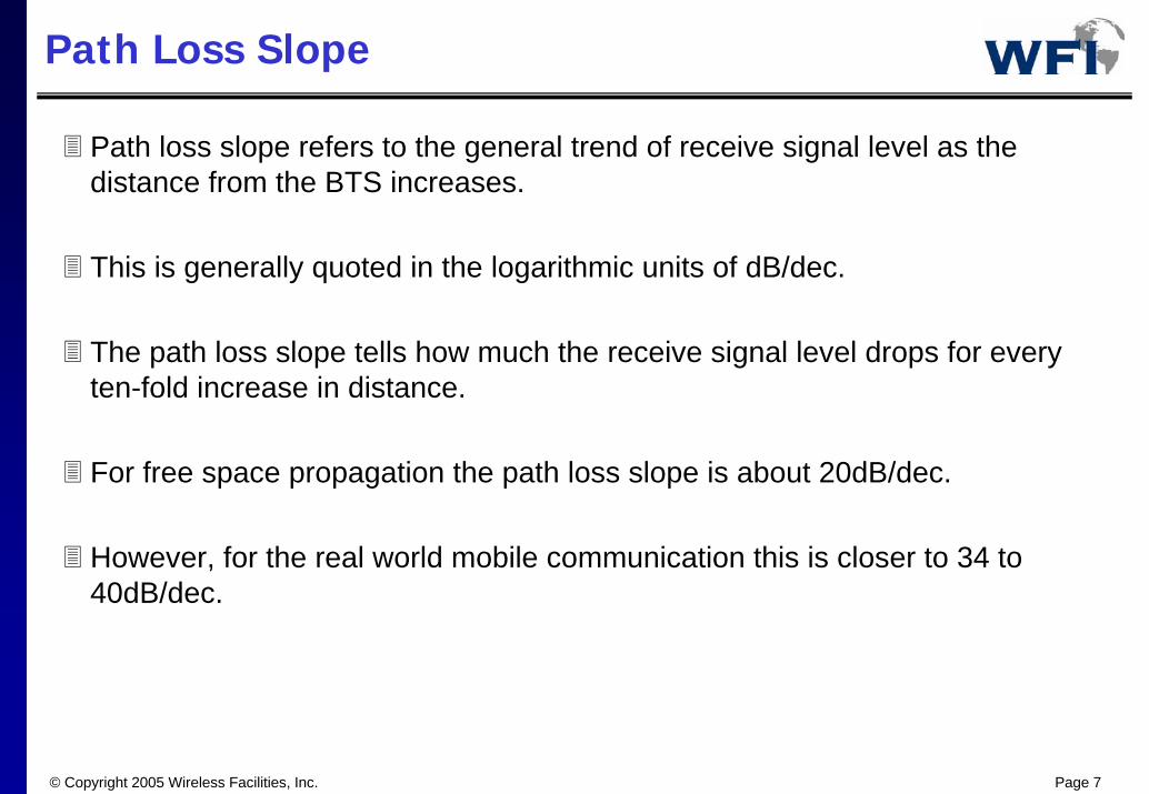
Path loss slope refers to the general trend of receive signal level as the distance from the BTS increases.
This is generally quoted in the logarithmic units of dB/dec.
The path loss slope tells how much the receive signal level drops for every ten-fold increase in distance.
For free space propagation the path loss slope is about 20dB/dec.
However, for the real world mobile communication this is closer to 34 to 40dB/dec.
© Copyright 2005 Wireless Facilities, Inc. Page 8
Mobile Radio Channel Model
Time/SpaceTime/Space
Sign
al P
ower
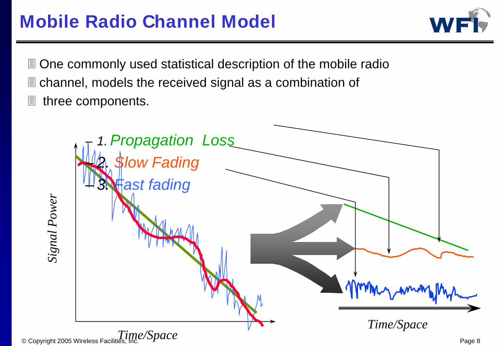
One commonly used statistical description of the mobile radio channel, models the received signal as a combination ofthree components.
– 1. Propagation Loss – 2. Slow Fading – 3. Fast fading

© Copyright 2005 Wireless Facilities, Inc. Page 9
Slow or Log Normal Fading
Actual received signal levels will deviate around the expected path loss slope.
These fades, or deviations, are mostly the result of terrain changes and the associated vehicle speed.
The nature of this fading has been shown to be log-normal with respect to the path loss slope. Hence, the statistical metric of standard deviation is often used to describe the amount of slow Fading. The standard deviation of this log-normal fading will depend on actual terrain;
however, a 5 to 8dB of standard deviation is generally accepted for “typical” terrain.
© Copyright 2005 Wireless Facilities, Inc. Page 10
Multi-path Fading (cont’d)
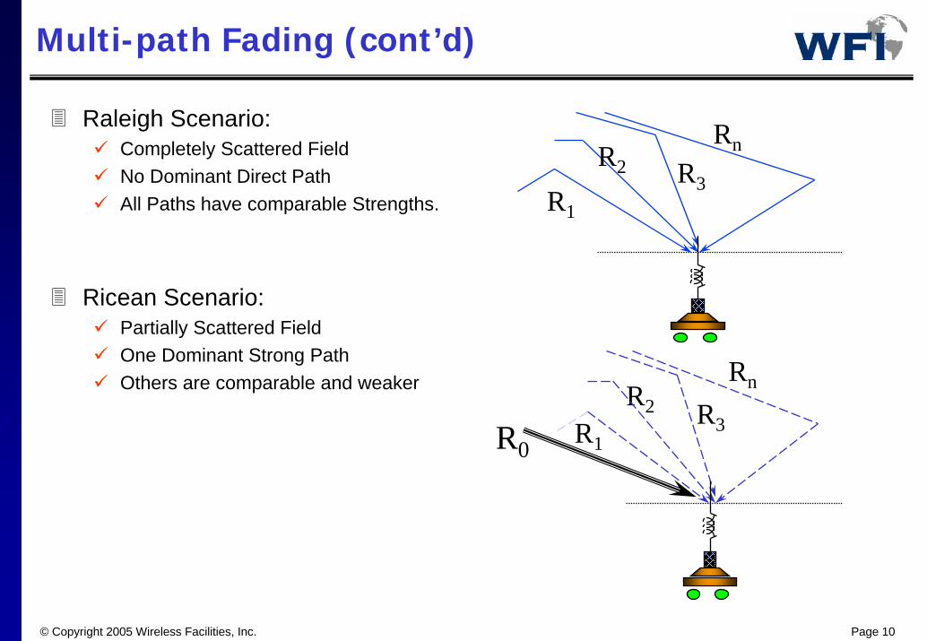
Raleigh Scenario:Completely Scattered FieldNo Dominant Direct PathAll Paths have comparable Strengths.
Ricean Scenario:Partially Scattered FieldOne Dominant Strong PathOthers are comparable and weaker
R1
R3R2
Rn
R1R3
R2
Rn
R0

© Copyright 2005 Wireless Facilities, Inc. Page 11
Hata’s Equation (review)
LHaUr(dB) = 69.55 + 26.l6 logfc - 13.82 log (hT) - a(hR) + [44.9 - 6.55 log hT)] log r -CF
The path loss for suburban areas is given byL ha,Su (dB) = L ha,Ur(dB) - 2[log fMHz/28]2 - 5.4
The path loss for open areas is given byL ha,Op(dB) = L ha,Ur(dB) - 4.78 [log fMHz]2 - 18.33log fMHz- 40.94
Range of Validity150 < fMHz < 15001 < rkm < 2030 < (hT)m< 200l < (hR)m < 10
© Copyright 2005 Wireless Facilities, Inc. Page 12
COST231-Hata Model (review)
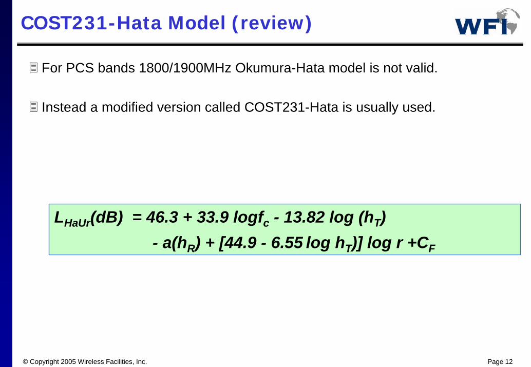
For PCS bands 1800/1900MHz Okumura-Hata model is not valid.
Instead a modified version called COST231-Hata is usually used.
LHaUr(dB) = 46.3 + 33.9 logfc - 13.82 log (hT) - a(hR) + [44.9 - 6.55 log hT)] log r +CF
© Copyright 2005 Wireless Facilities, Inc. Page 13
Multi-path and Fading Effects
Multi-path and fading effects determine the small distance/ short time power variations.
Multi-path delay leads to two undesirable effects:
Fading, treated mainly by diversity in the receiver.
Inter-symbol interference, which is treated mainly by using an adaptive equalizer.
© Copyright 2005 Wireless Facilities, Inc. Page 14
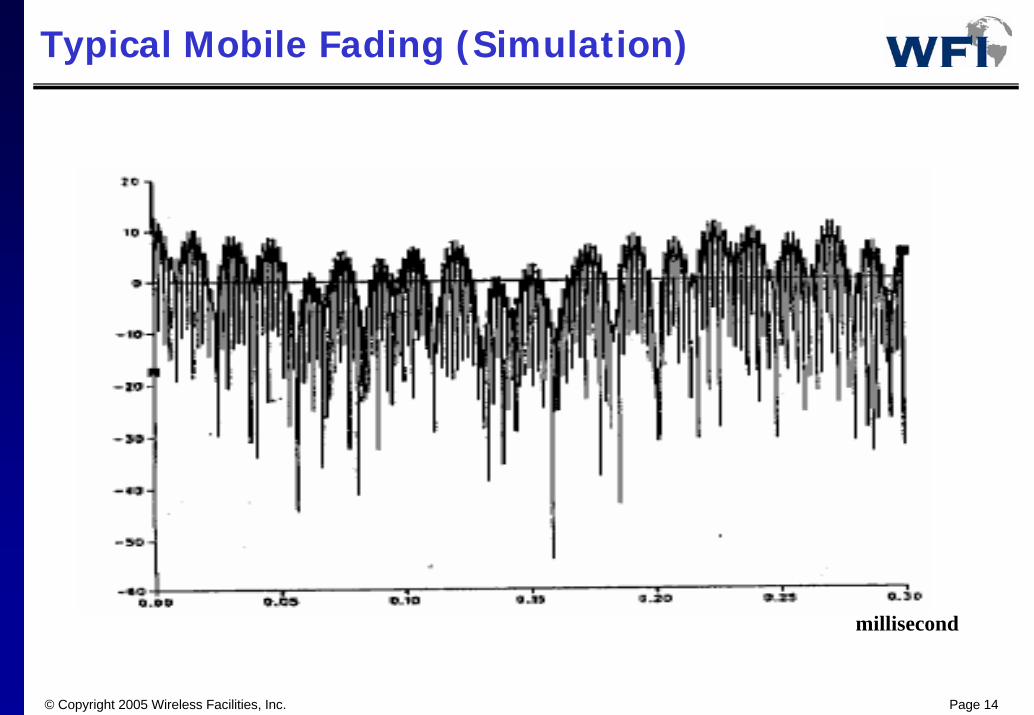
Typical Mobile Fading (Simulation)
millisecond
© Copyright 2005 Wireless Facilities, Inc. Page 15
Multiple Wave Fading
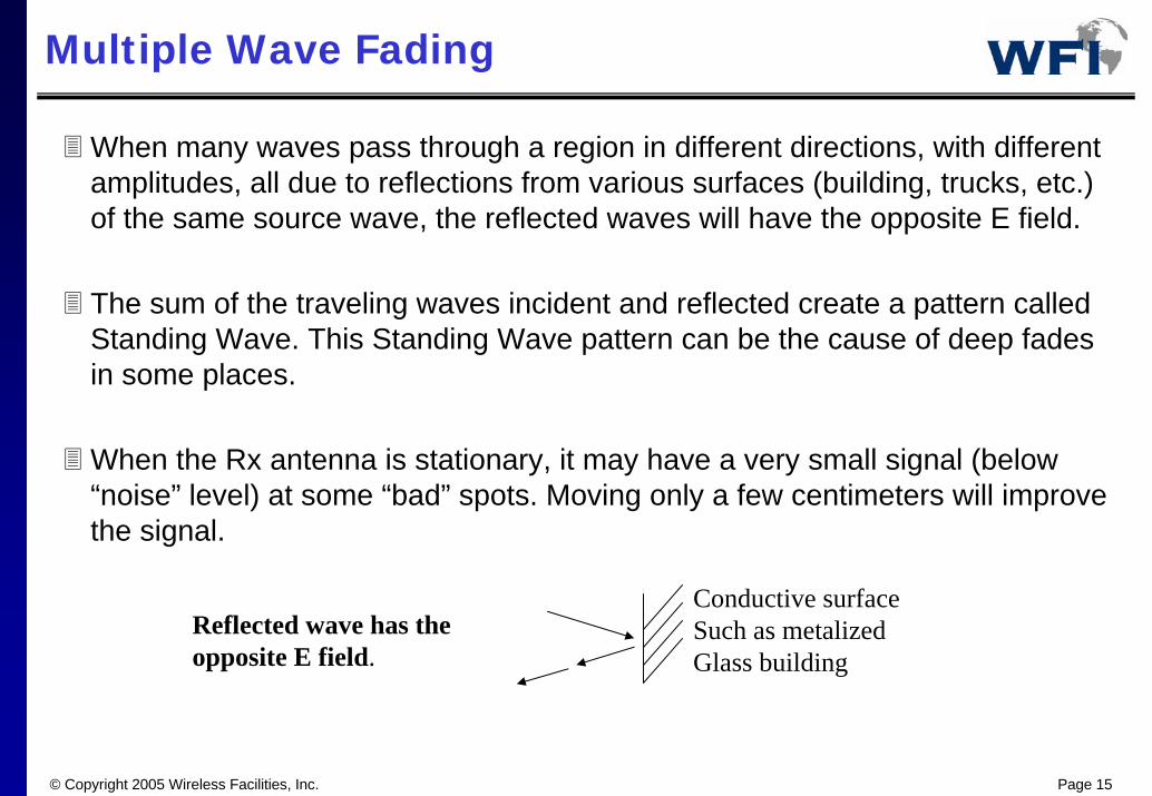
When many waves pass through a region in different directions, with different amplitudes, all due to reflections from various surfaces (building, trucks, etc.) of the same source wave, the reflected waves will have the opposite E field.
The sum of the traveling waves incident and reflected create a pattern called Standing Wave. This Standing Wave pattern can be the cause of deep fades in some places.
When the Rx antenna is stationary, it may have a very small signal (below “noise” level) at some “bad” spots. Moving only a few centimeters will improve the signal.
Reflected wave has the opposite E field.
Conductive surface Such as metalizedGlass building
© Copyright 2005 Wireless Facilities, Inc. Page 16
Multiple Wave Fading (cont’d)
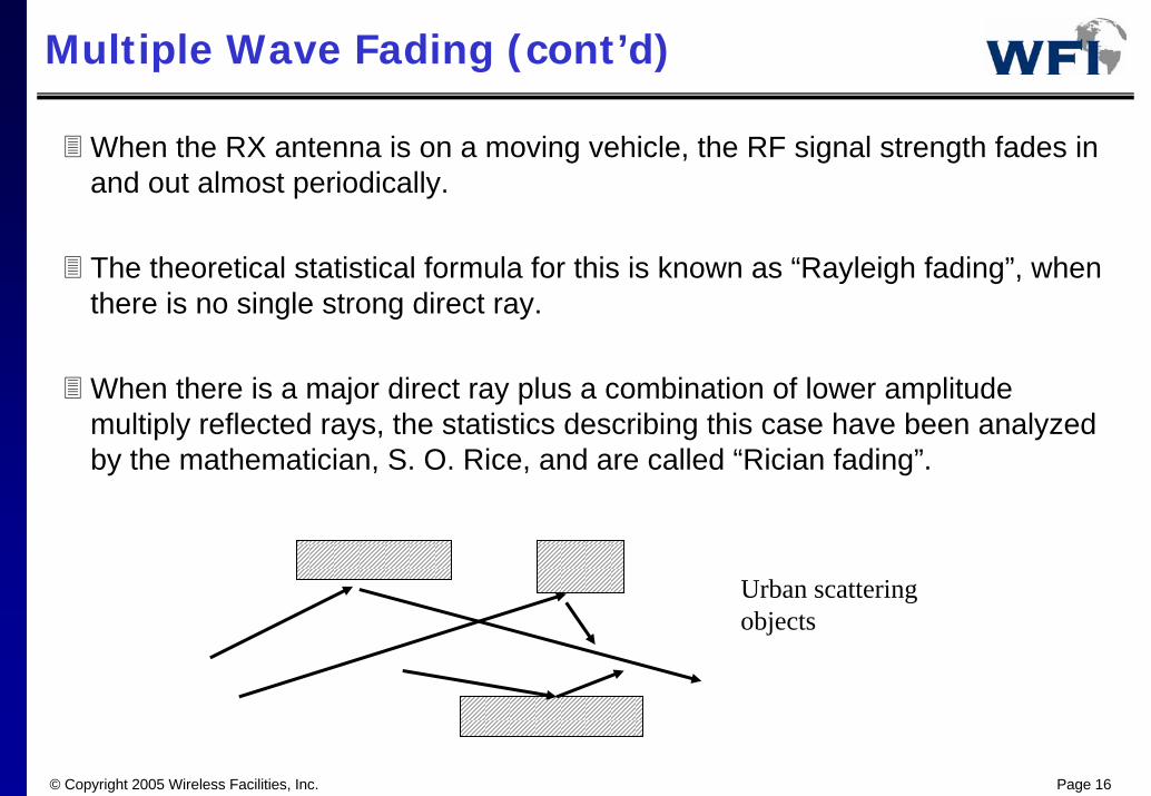
When the RX antenna is on a moving vehicle, the RF signal strength fades in and out almost periodically.
The theoretical statistical formula for this is known as “Rayleigh fading”, when there is no single strong direct ray.
When there is a major direct ray plus a combination of lower amplitude multiply reflected rays, the statistics describing this case have been analyzed by the mathematician, S. O. Rice, and are called “Rician fading”.
Urban scatteringobjects
© Copyright 2005 Wireless Facilities, Inc. Page 17
Diversity
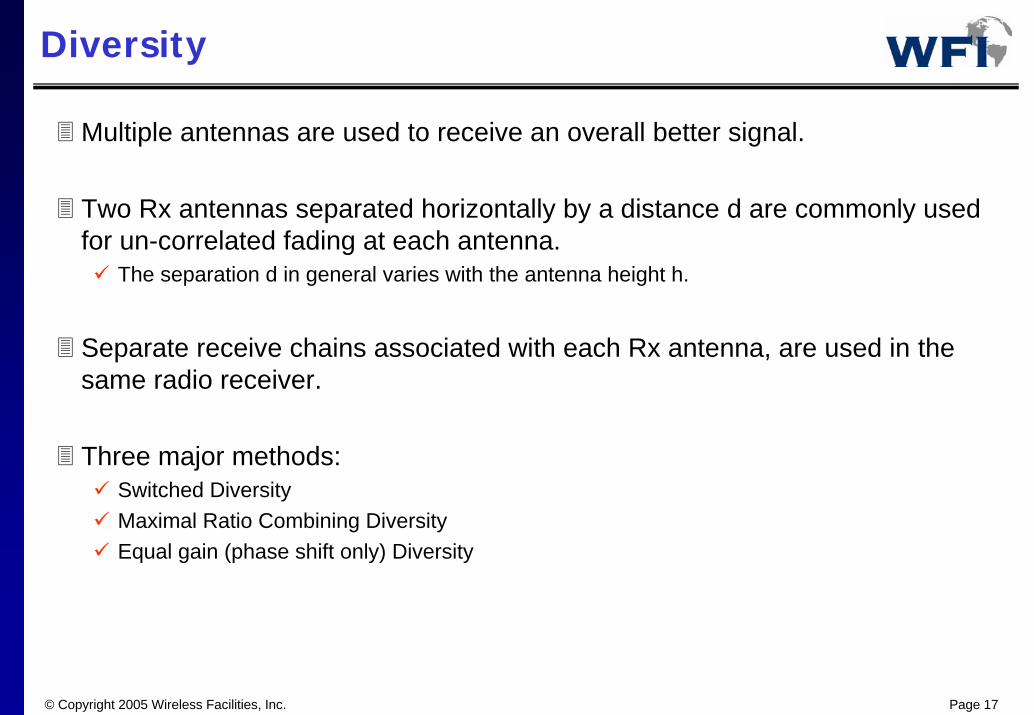
Multiple antennas are used to receive an overall better signal.
Two Rx antennas separated horizontally by a distance d are commonly used for un-correlated fading at each antenna.
The separation d in general varies with the antenna height h.
Separate receive chains associated with each Rx antenna, are used in the same radio receiver.
Three major methods:Switched DiversityMaximal Ratio Combining DiversityEqual gain (phase shift only) Diversity

© Copyright 2005 Wireless Facilities, Inc. Page 18
Diversity (cont’d)
Time
Sign
al L
evel
in d
B
Signal A Signal B Combined Signal
After reception the two signals can be combined and the fade smoothed out before the message is detected.
Addition of two equal strength RF carriers doubles the voltage, quadruples signal power, while incoherent addition of noise signals only doubles noise power. Signal to noise ratio improves by 4/2=2(3dB).
© Copyright 2005 Wireless Facilities, Inc. Page 19
Switched Diversity
“Front end”Receiver
“Front end”Receiver
Antenna B
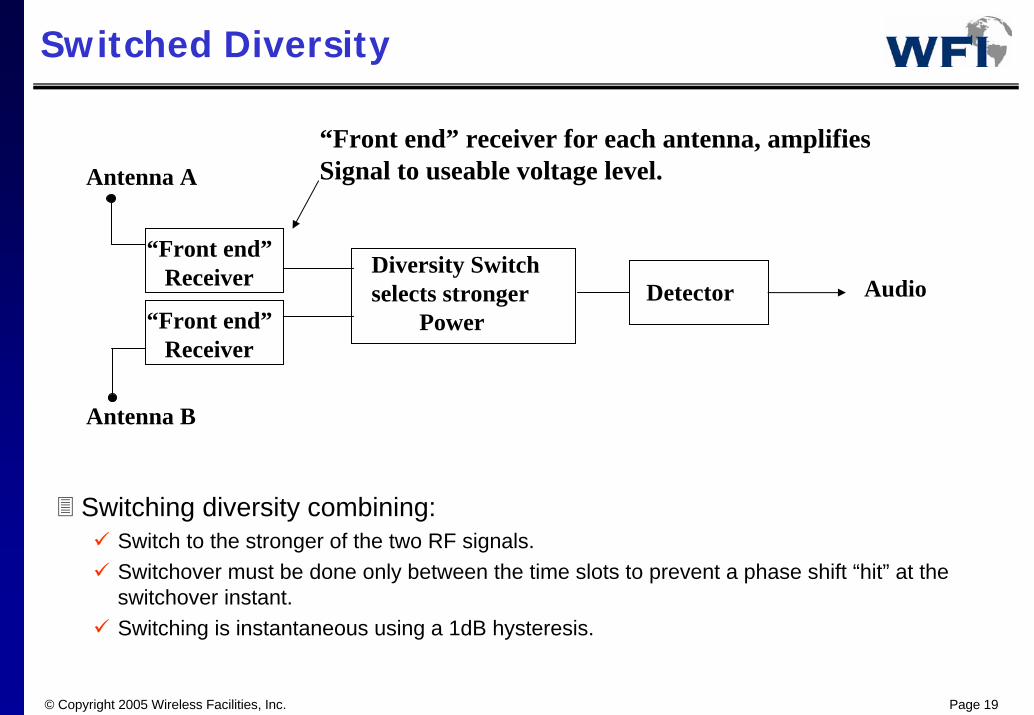
Diversity Switchselects stronger
PowerDetector
“Front end” receiver for each antenna, amplifiesSignal to useable voltage level.Antenna A
Audio
Switching diversity combining:Switch to the stronger of the two RF signals.Switchover must be done only between the time slots to prevent a phase shift “hit” at the switchover instant.Switching is instantaneous using a 1dB hysteresis.
© Copyright 2005 Wireless Facilities, Inc. Page 20
Equal Gain Diversity
“Front end”Receiver
Antenna A
“Front end”Receiver
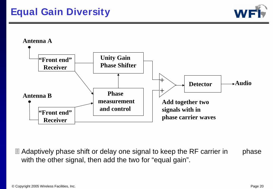
Unity GainPhase Shifter
Antenna B
Detector Audio
Phase measurementand control
++Add together twosignals with in phase carrier waves
Adaptively phase shift or delay one signal to keep the RF carrier in phase with the other signal, then add the two for “equal gain”.
© Copyright 2005 Wireless Facilities, Inc. Page 21
Maximal Ratio Diversity
“Front end”Receiver
“Front end”Receiver
Antenna A
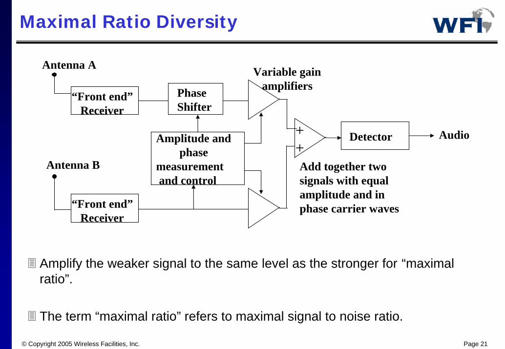
Phase Shifter
DetectorAmplitude andphase
measurementand control
++Add together twosignals with equal amplitude and inphase carrier waves
Variable gainamplifiers
Amplify the weaker signal to the same level as the stronger for “maximal ratio”.
The term “maximal ratio” refers to maximal signal to noise ratio.
Audio
Antenna B
© Copyright 2005 Wireless Facilities, Inc. Page 22
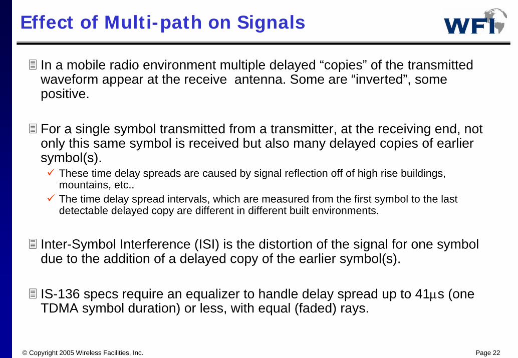
Effect of Multi-path on Signals
In a mobile radio environment multiple delayed “copies” of the transmitted waveform appear at the receive antenna. Some are “inverted”, some positive.
For a single symbol transmitted from a transmitter, at the receiving end, not only this same symbol is received but also many delayed copies of earlier symbol(s).
These time delay spreads are caused by signal reflection off of high rise buildings, mountains, etc.. The time delay spread intervals, which are measured from the first symbol to the last detectable delayed copy are different in different built environments.
Inter-Symbol Interference (ISI) is the distortion of the signal for one symbol due to the addition of a delayed copy of the earlier symbol(s).
IS-136 specs require an equalizer to handle delay spread up to 41µs (one TDMA symbol duration) or less, with equal (faded) rays.
© Copyright 2005 Wireless Facilities, Inc. Page 23
ISI and Equalizer Action

© Copyright 2005 Wireless Facilities, Inc. Page 24
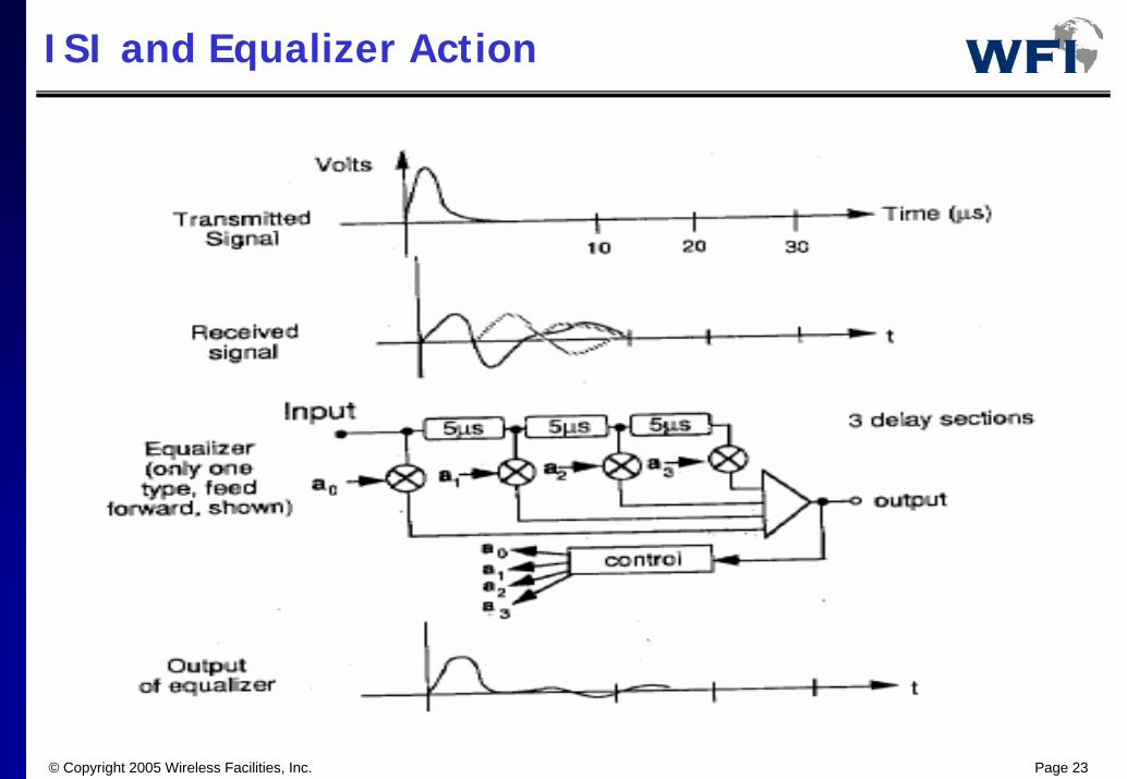
ISI and Equalizer Action
Control box in the equalizer adjusts the tap coefficients a0, a1, a2, a3 to produce minimum ISI during the SYNCH or CDVCC bit stream input interval of the TDMA frame.
Control box continues to make small adjustments in a0, a1, a2, a3 during data reception, to keep the symbol values as close as possible to design levels.

© Copyright 2005 Wireless Facilities, Inc. Page 25
Doppler Shift
When the mobile station moves towards the base, the RF frequency seen by the receiver increases.
When the mobile station moves away from the base, the RF frequency seen by the receiver decreases.
This is the result of Doppler effect, the same physical phenomenon that makes the pitch of a train whistle appear to go up and then down as the train moves toward and then away from you.
For a 100Km/h speed at 1900Mhz, the frequency shift can be +/-176Hz or more.
f’ = f [1+ (v/c) cos θ]
This is usually corrected at the equalizer to prevent false PM.
© Copyright 2005 Wireless Facilities, Inc. Page 26
Link Budget
© Copyright 2005 Wireless Facilities, Inc. Page 27
Link Budget Overview
The link budget will provide an analysis of the communication link between the base station (BTS) and the mobile (MS), and it is one of the first activities performed within the design process.
The link budget will take the coverage objective, the technology and propagation assumption and provide guidelines for:
the average cell radii, BTS transmit powers, and the signal levels which define the cell edge.
© Copyright 2005 Wireless Facilities, Inc. Page 28
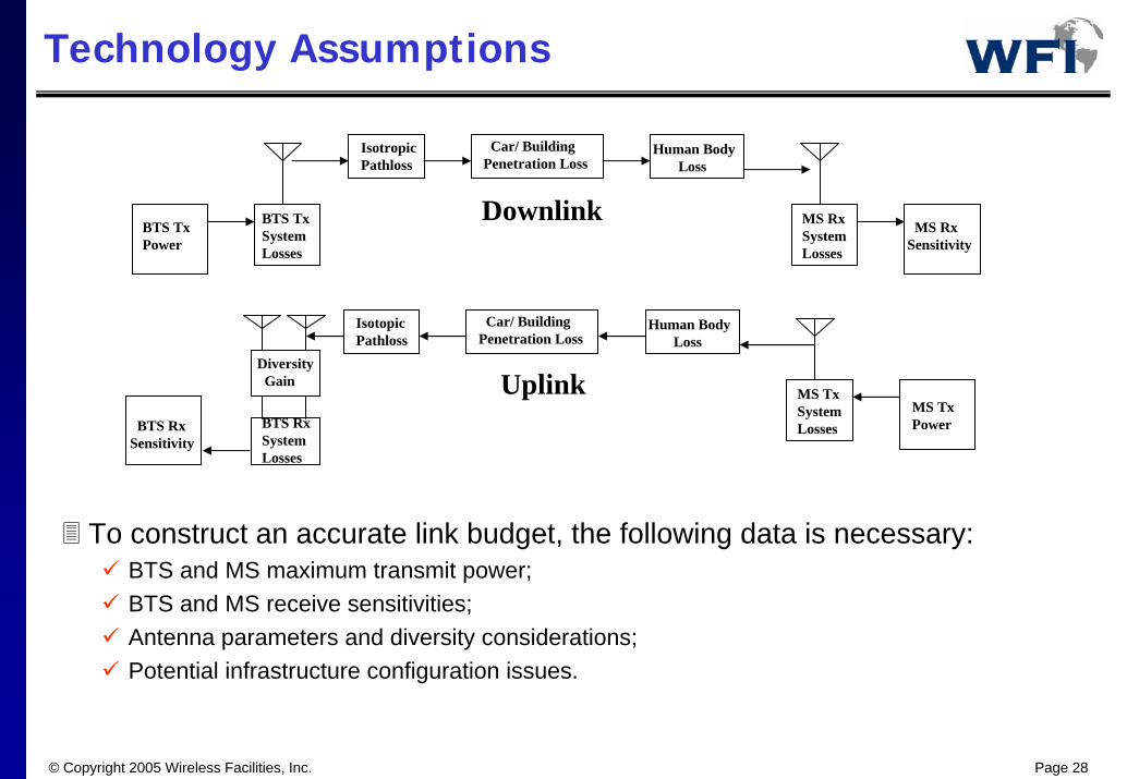
Technology Assumptions
BTS TxPower
BTS TxSystem Losses
IsotropicPathloss
Car/ BuildingPenetration Loss
Human BodyLoss
MS RxSystem Losses
MS RxSensitivity
Downlink
MS TxPowerBTS Rx
System Losses
IsotopicPathloss
Car/ BuildingPenetration Loss
Human BodyLoss
MS TxSystem LossesBTS Rx
Sensitivity
UplinkDiversity
Gain
To construct an accurate link budget, the following data is necessary:BTS and MS maximum transmit power;BTS and MS receive sensitivities;Antenna parameters and diversity considerations;Potential infrastructure configuration issues.
© Copyright 2005 Wireless Facilities, Inc. Page 29
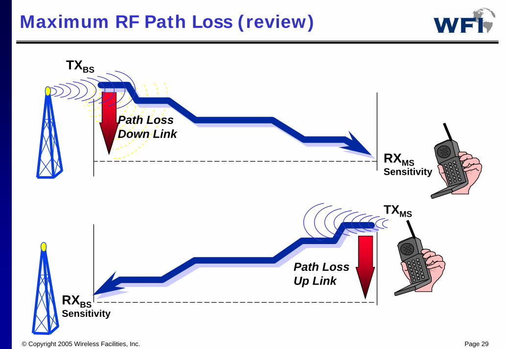
Maximum RF Path Loss (review)
RXBSSensitivity
RXMSSensitivity
Path Loss Down Link
Path Loss Up Link
TXBS
TXMS
© Copyright 2005 Wireless Facilities, Inc. Page 30
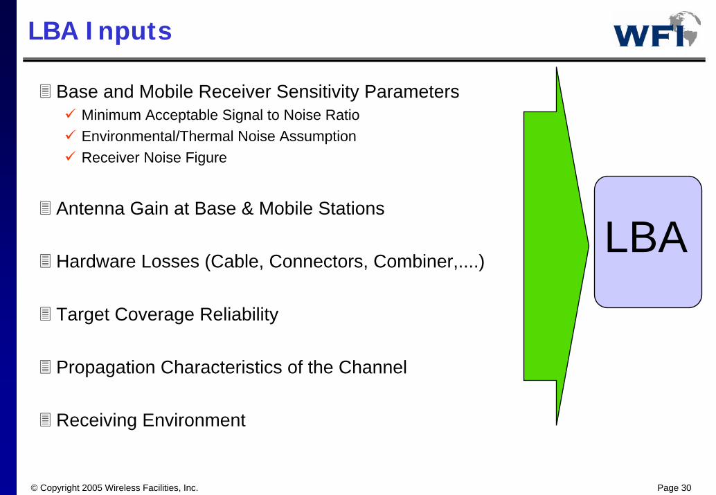
LBA Inputs
Base and Mobile Receiver Sensitivity ParametersMinimum Acceptable Signal to Noise Ratio Environmental/Thermal Noise AssumptionReceiver Noise Figure
Antenna Gain at Base & Mobile Stations
Hardware Losses (Cable, Connectors, Combiner,....)
Target Coverage Reliability
Propagation Characteristics of the Channel
Receiving Environment
LBA
© Copyright 2005 Wireless Facilities, Inc. Page 31
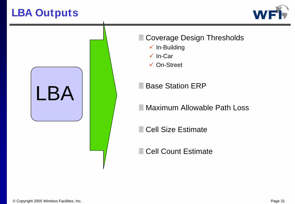
LBA Outputs
Coverage Design ThresholdsIn-BuildingIn-CarOn-Street
Base Station ERP
Maximum Allowable Path Loss
Cell Size Estimate
Cell Count Estimate
LBA
© Copyright 2005 Wireless Facilities, Inc. Page 32
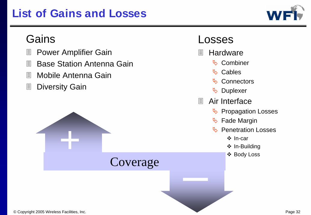
List of Gains and Losses
GainsPower Amplifier GainBase Station Antenna GainMobile Antenna GainDiversity Gain
Losses Hardware
CombinerCablesConnectorsDuplexer
Air InterfacePropagation LossesFade MarginPenetration Losses
In-carIn-BuildingBody Loss+
Coverage
© Copyright 2005 Wireless Facilities, Inc. Page 33
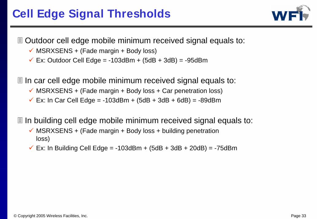
Cell Edge Signal Thresholds
Outdoor cell edge mobile minimum received signal equals to:MSRXSENS + (Fade margin + Body loss)Ex: Outdoor Cell Edge = -103dBm + (5dB + 3dB) = -95dBm
In car cell edge mobile minimum received signal equals to:MSRXSENS + (Fade margin + Body loss + Car penetration loss)Ex: In Car Cell Edge = -103dBm + (5dB + 3dB + 6dB) = -89dBm
In building cell edge mobile minimum received signal equals to:MSRXSENS + (Fade margin + Body loss + building penetration loss)Ex: In Building Cell Edge = -103dBm + (5dB + 3dB + 20dB) = -75dBm
© Copyright 2005 Wireless Facilities, Inc. Page 34
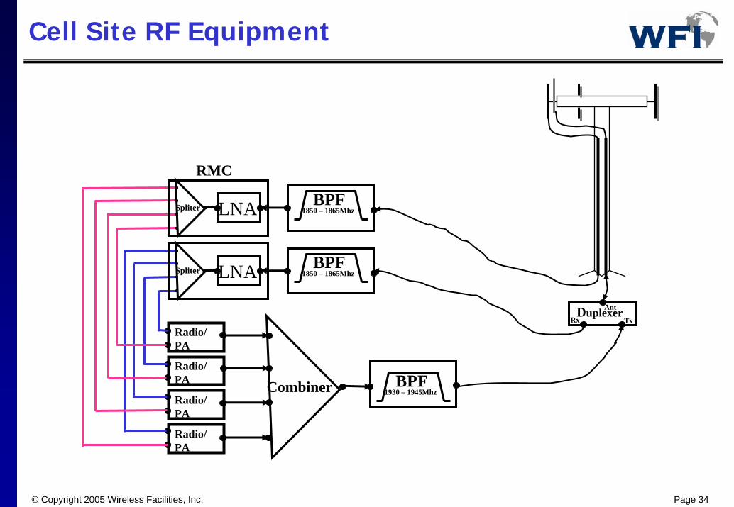
Cell Site RF Equipment
DuplexerAnt
TxRx
Radio/ PA
Radio/ PA
Radio/ PA
Radio/ PA
Combiner 1930 – 1945MhzBPF
1850 – 1865MhzBPFSpliter LNA
1850 – 1865MhzBPFSpliter LNA
RMC
© Copyright 2005 Wireless Facilities, Inc. Page 35
BTS Hardware Components
Antenna
Duplexor
Receiver Multicoupler
Power Amplifier
Transmit Combiner
Master Oscillator
Radio Receiver and Transmitter
© Copyright 2005 Wireless Facilities, Inc. Page 36
Antenna Parameter
An antenna is a passive device which acts as to focus energy.
It does not amplify RF energy, but merely redirect it.
The important antenna characteristics are: Gain, Horizontal and Vertical beam width, andDiversity performance.
The gain and beam width parameters are interrelated and usually come at the expense of one another.
With regard to antenna reception these parameters quantify the amount of energy that the antenna is able to collect in a particular direction. With regard to transmission, they indicate the amount of power transmitted in a particular direction.
© Copyright 2005 Wireless Facilities, Inc. Page 37
Antenna Gain
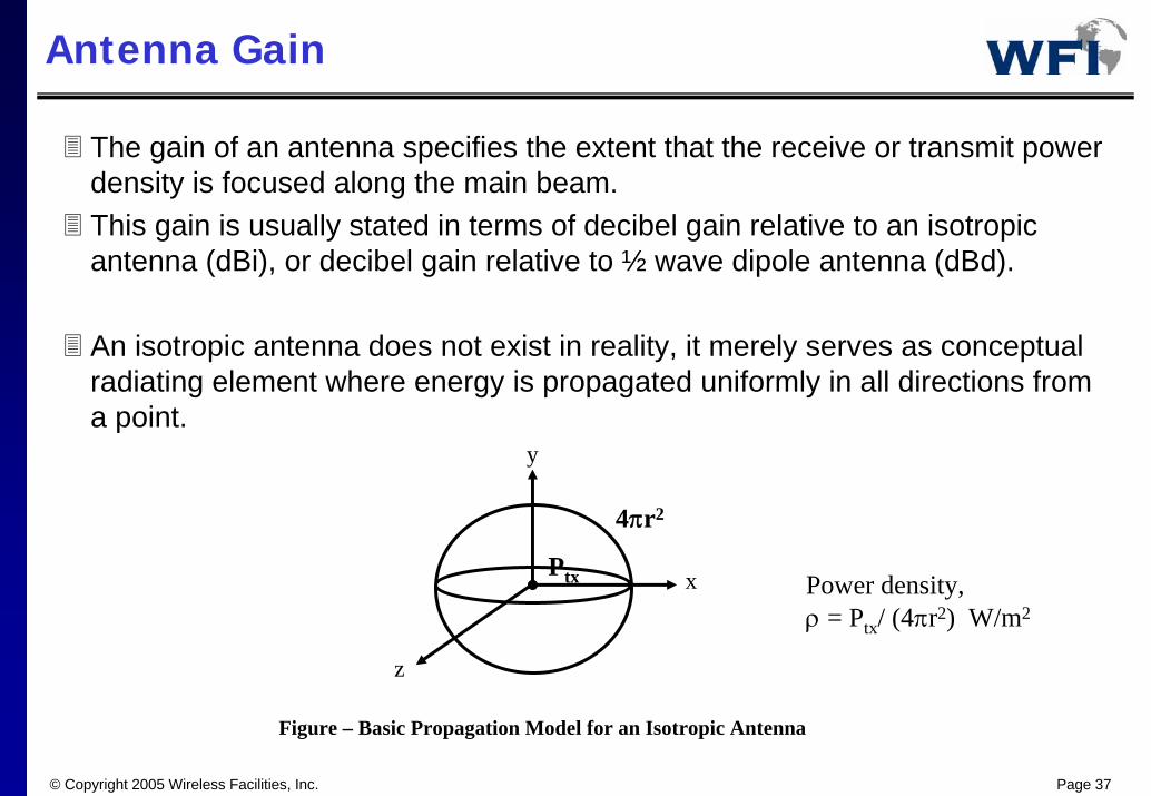
The gain of an antenna specifies the extent that the receive or transmit power density is focused along the main beam. This gain is usually stated in terms of decibel gain relative to an isotropic antenna (dBi), or decibel gain relative to ½ wave dipole antenna (dBd).
An isotropic antenna does not exist in reality, it merely serves as conceptual radiating element where energy is propagated uniformly in all directions from a point.
Figure – Basic Propagation Model for an Isotropic Antenna
Power density,ρ = Ptx/ (4πr2) W/m2
x
y
z
Ptx
4πr2

© Copyright 2005 Wireless Facilities, Inc. Page 38
Antenna Beam width
Sectored antennas are commonly used in a mobile environment.
They focus energy within a particular angle in the horizontal plane.
Horizontal Beam width describes the horizontal angle within which the gain of the antenna does not drop below 3dB from the beam gain.
Vertical Beam width describes the vertical angle within which the gain of the antenna does not drop below 3dB from the main beam gain.
© Copyright 2005 Wireless Facilities, Inc. Page 39
Diversity Performance
Receive diversity at the cell site can be used to improve mobile reception and coverage reliability.
Space diversity is commonly used in the mobile environment which uses receive antenna separation to help minimize the effect of Rayleigh fading on the up link.
Rayleigh fading is a consequence of multiple copies of the same signal combining de-constructively at the receive antenna.
By using two or more antennas separated in space, it increases the probability that both antennas will not experience fades simultaneously.

© Copyright 2005 Wireless Facilities, Inc. Page 40
Duplexor
Allows transmitter and receiver to share one antenna.
Uses broadband resonant filters to keep high transmit RF power from entering the receiver chain.

© Copyright 2005 Wireless Facilities, Inc. Page 41
Band Pass Filter
It Is used to suppress the unwanted signals outside the desired receive or transmit band.
© Copyright 2005 Wireless Facilities, Inc. Page 42
Multi-coupler
It is used to amplify and couple the signal received from the antenna to the receivers.
It includes an LNA and a power splitter.

© Copyright 2005 Wireless Facilities, Inc. Page 43
Power Amplifier (PA)
It is used to amplify the output of a radio transmitter from about 10mW to 30W.
© Copyright 2005 Wireless Facilities, Inc. Page 44
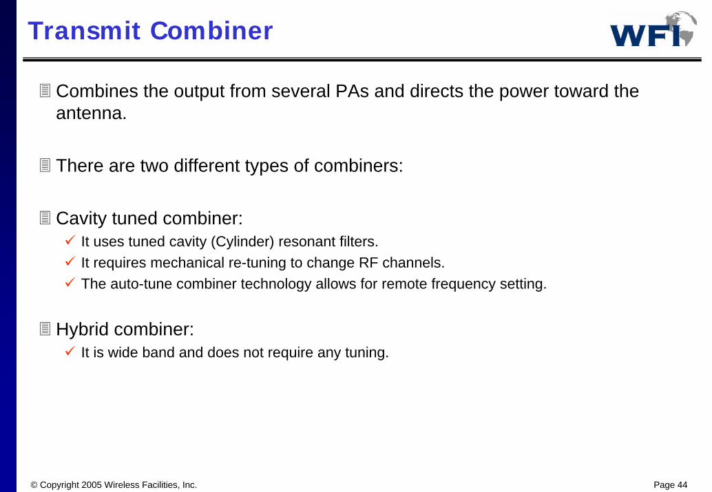
Transmit Combiner
Combines the output from several PAs and directs the power toward the antenna.
There are two different types of combiners:
Cavity tuned combiner:It uses tuned cavity (Cylinder) resonant filters. It requires mechanical re-tuning to change RF channels. The auto-tune combiner technology allows for remote frequency setting.
Hybrid combiner:It is wide band and does not require any tuning.
© Copyright 2005 Wireless Facilities, Inc. Page 45
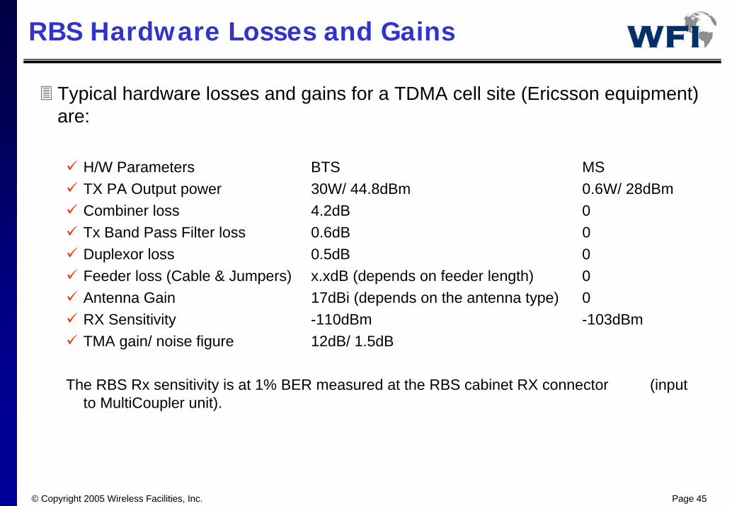
RBS Hardware Losses and Gains
Typical hardware losses and gains for a TDMA cell site (Ericsson equipment) are:
H/W Parameters BTS MSTX PA Output power 30W/ 44.8dBm 0.6W/ 28dBmCombiner loss 4.2dB 0Tx Band Pass Filter loss 0.6dB 0Duplexor loss 0.5dB 0Feeder loss (Cable & Jumpers) x.xdB (depends on feeder length) 0Antenna Gain 17dBi (depends on the antenna type) 0RX Sensitivity -110dBm -103dBmTMA gain/ noise figure 12dB/ 1.5dB
The RBS Rx sensitivity is at 1% BER measured at the RBS cabinet RX connector (input to MultiCoupler unit).

© Copyright 2005 Wireless Facilities, Inc. Page 46
RBS Hardware
DuplexerAnt
TxRx
Radio/ PA
Radio/ PA
Radio/ PA
Radio/ PA
Combiner 1930 – 1945MhzBPF
1850 – 1865MhzBPFSpliter LNA
1850 – 1865MhzBPFSpliter LNA
RMC
© Copyright 2005 Wireless Facilities, Inc. Page 47
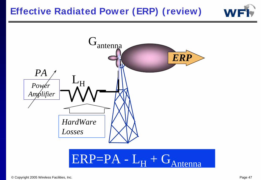
Effective Radiated Power (ERP) (review)
Power Amplifier
HardWareLosses
PA LH
GantennaERP
ERP=PA - LH + GAntenna

© Copyright 2005 Wireless Facilities, Inc. Page 48
Receiver Sensitivity (review)
LNA
RX: Receiver sensitivityIs the minimum acceptable input signal level in dBm, at the input of the receiver’s low noise amplifier, required by the system for reliable communication.
RX is a function of:Carrier to Noise Ratio (CNR)
For a given FER, e.g. of about 1%, each type of modulation and coding requires a minimum signal to noise ratio which at the bit level is stated as Eb/No.
Thermal/Environmental Noise: Is a combination of
– Antenna Noise (dBm)– Receiver Noise Figure(NF) in dB– Temperature and System Bandwidth
© Copyright 2005 Wireless Facilities, Inc. Page 49
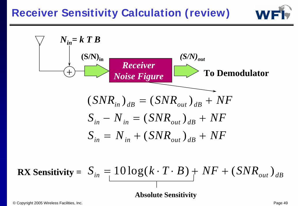
Receiver Sensitivity Calculation (review)
ReceiverNoise Figure
Nin= k T B
(S/N)out(S/N)in
Absolute Sensitivity
RX Sensitivity =
( ) ( )( )( )
log( ) ( )
SNR SNR NFS N SNR NFS N SNR NF
S k T B NF SNR
in dB out dB
in in out dB
in in out dB
in out dB
= +− = += + +
= ⋅ ⋅ + +10
To Demodulator+

© Copyright 2005 Wireless Facilities, Inc. Page 50
Penetration Losses (review)
In-Car
On StreetIn CarIn BuildingBody Loss
© Copyright 2005 Wireless Facilities, Inc. Page 51
Coverage Objective
The term coverage refers to an area having sufficiently strong signal level on both the uplink and downlink that a user can originate a call with acceptable voice quality in both directions.
Coverage requirements are usually stated as:
The need for in building, in car, or outdoor coverage.
The probability of coverage at the cell edge and over the cell area.
© Copyright 2005 Wireless Facilities, Inc. Page 52
Contour Coverage Reliability
Normal Distribution
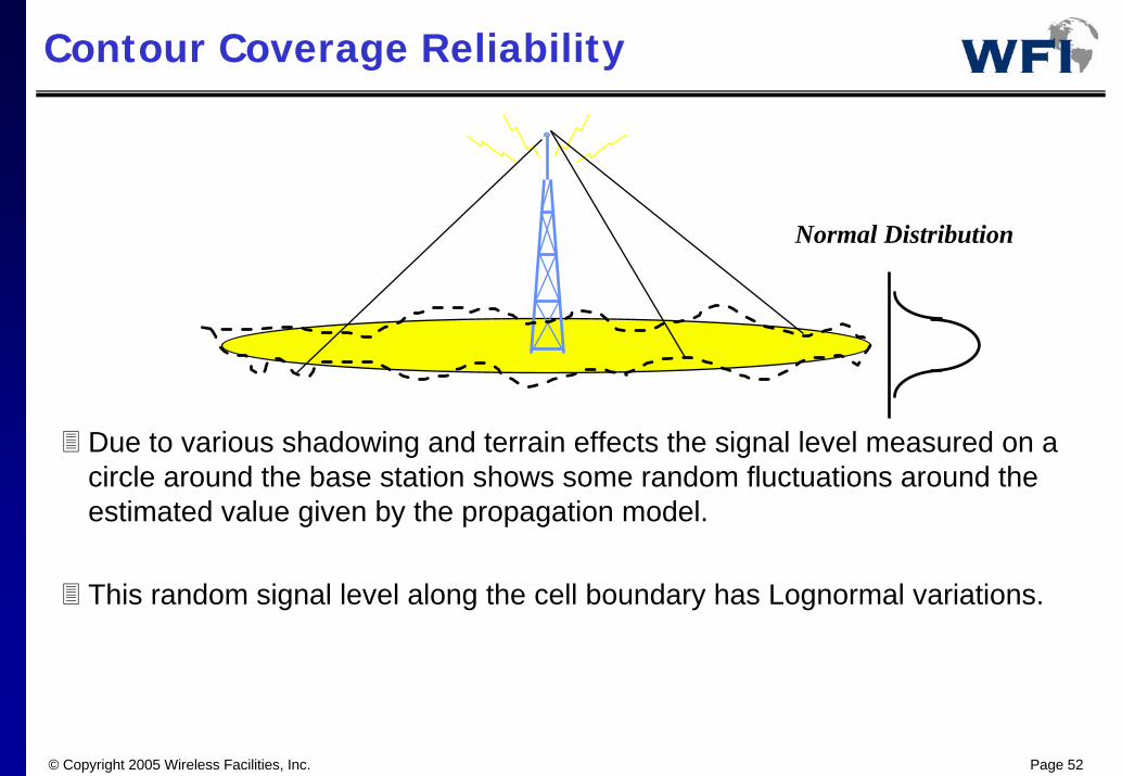
Due to various shadowing and terrain effects the signal level measured on a circle around the base station shows some random fluctuations around the estimated value given by the propagation model.
This random signal level along the cell boundary has Lognormal variations.

© Copyright 2005 Wireless Facilities, Inc. Page 53
Coverage Probability
Cell area coverage:Refers to the percentage of average useable area by the cell site. This perspective would provide an estimate of successful origination of a call, if the user were to attempt calls at a random positions within the cell boundary.
Cell edge criteria:Gives the threshold of acceptable performance. This perspective will define the cell edge as the distance where a serving cell site can no longer provide a minimum service reliability. As a result, the cell edge will establish an area within which most of the points should have a probability of coverage greater than threshold.
© Copyright 2005 Wireless Facilities, Inc. Page 54
Fast or Rayleigh Fading
Fast fading occurs at a much quicker rate than its log-normal counterpart.
Fast fading is the result of signals reflecting off of man made objects and taking different paths from the transmitter to the receiver.
Because of path differential, similar signals can arrive at the receiver at different times and cause constructive and deconstructive condition.
Fading due to multi-path reflections can be shown to have Rayleighdistribution.
Although Rayleigh fading is present in most environments, its effect is normally not considered by propagation models.
One reason being that it would be difficult to build a database of all man made structures.
© Copyright 2005 Wireless Facilities, Inc. Page 55
Fade Margin Calculation
The process of engineering a cell coverage involves uncertainty as a propagation model with associated error is used to predict signal levels for a certain area.
To combat the uncertainty involved with propagation prediction, a fade margin is used to pad the link budget and provide a confidence factor that a sufficient signal level will be present a certain percentage of the time.
Many natural processes can be characterized by a normal distribution.
A normal distribution can be fully characterized by its mean and standard deviation.
Standard deviation:Statistically speaking, it is used in conjunction with a normal distribution to show how spread out the population of outcomes are with respect to its mean.

© Copyright 2005 Wireless Facilities, Inc. Page 56
Fade Margin Calculation (cont’d)
When applied to RF propagation modeling, standard deviation provides a statistical metric that helps to quantify the uncertainty involved with the model.
As discussed before, 5 to 8 dB of slow fading standard deviation is typically assumed for normal terrain.
This can also be viewed as prediction error.
© Copyright 2005 Wireless Facilities, Inc. Page 57
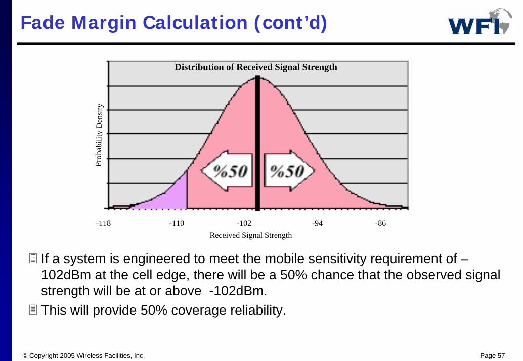
Fade Margin Calculation (cont’d)
-118 -110 -102 -94 -86
Distribution of Received Signal Strength
Received Signal Strength
Prob
abili
t y D
ensi
ty
If a system is engineered to meet the mobile sensitivity requirement of –102dBm at the cell edge, there will be a 50% chance that the observed signal strength will be at or above -102dBm. This will provide 50% coverage reliability.

© Copyright 2005 Wireless Facilities, Inc. Page 58
Fade Margin Calculation (cont’d)
-110 -102 -94 -86 -78
Distribution of Received Signal Strength
Received Signal Strength
Prob
abili
t y D
ensi
ty
%85%15
The incorporation of a fade margin provides increased cell edge reliability. In the above case, defining the cell edge at –94dBm will provide a 85% probability that the actual received signal strength will be above the –102dBm at the cell edge.
This means that a signal can fade 8dB more than the propagation model had expected without dipping below the mobile receive sensitivity.

© Copyright 2005 Wireless Facilities, Inc. Page 59
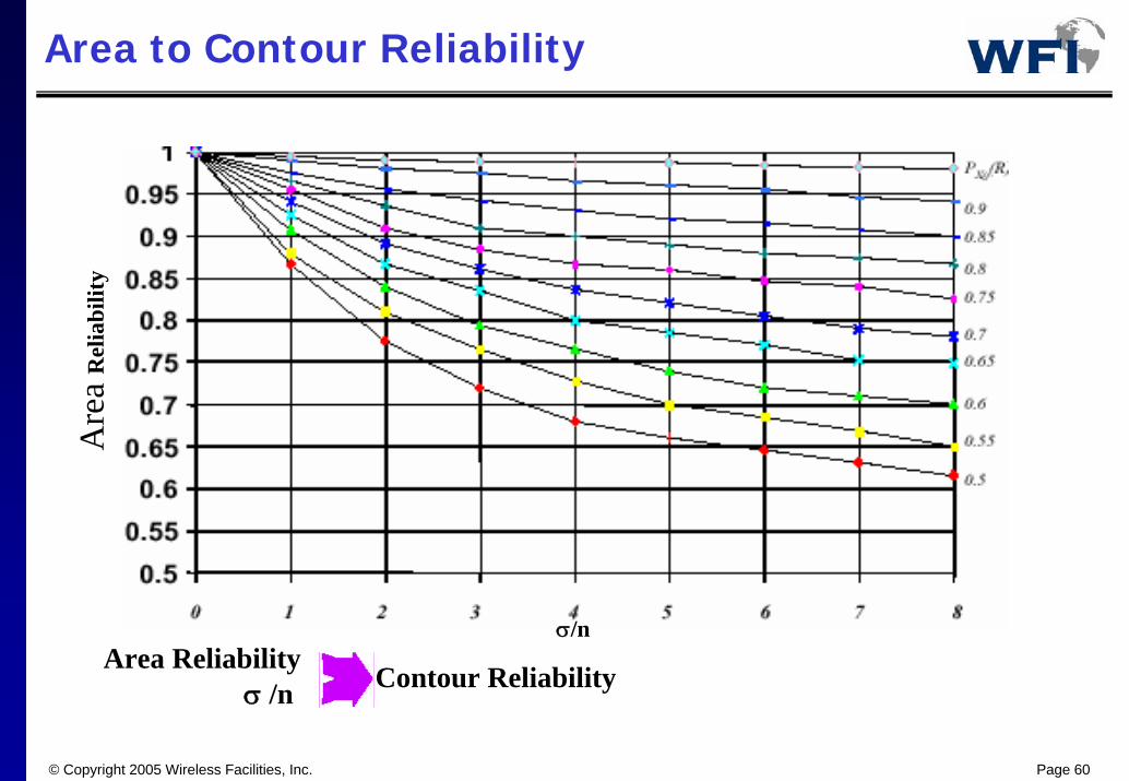
Area Coverage Reliability
Coverage design objectives are usually defined in terms of area reliability. Area reliability is the percentage of area where the received signal is above the threshold. It can be thought of as the average of contour reliability for all circles of radii r, 0 < r < R.
© Copyright 2005 Wireless Facilities, Inc. Page 60
Area to Contour ReliabilityA
rea
Rel
iabi
lity
σ/n
Contour ReliabilityArea Reliability
σ /n
© Copyright 2005 Wireless Facilities, Inc. Page 61
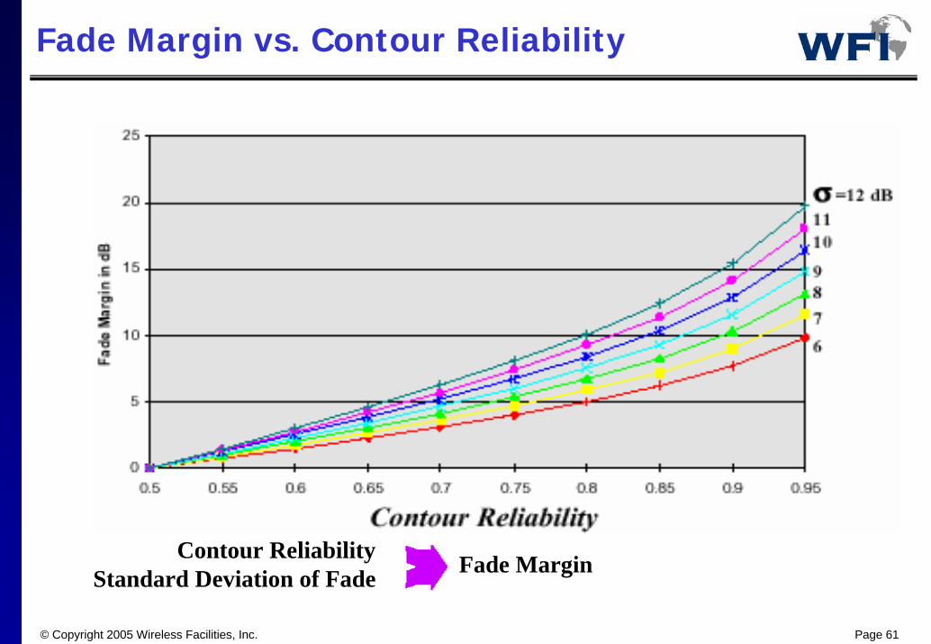
Fade Margin vs. Contour Reliability
Contour ReliabilityStandard Deviation of Fade Fade Margin

© Copyright 2005 Wireless Facilities, Inc. Page 62
Fade Margin Calculation
For a given
Standard Deviation, σ (urban: σ =5dB, suburban: σ = 6dB, rural: σ = 7dB).
The propagation loss factor, n (Note: A typical propagation loss factor is n = 3.5);
Compute σ /n.
For the required area reliability and computed σ /n
Estimate coverage contour reliability from plot 1 (Area to Contour Reliability)
Use the contour reliability, the standard deviation, σ, and plot 2 (Fade Margin vs. Contour Reliability) to estimate the fade margin.

© Copyright 2005 Wireless Facilities, Inc. Page 63
Down Link Budget CalculationFor sites with short feeder line
BTS EIRP:BTSTX_EIRP = BTSTXPA_OutputPower – BTSTX _SystemLoss +
BTSTX_AntennaGain
Where:BTSTX _SystemLoss = (Combiner loss + TX Filter loss) + Duplexor loss + Feeder loss
= (4.2dB + 0.6dB) + 0.5dB + 2.5dB = 7.8dB
BTSTX_EIRP = 44.8dBm – 7.8dB + 17dBi = 54dBm
This is the maximum EIRP attainable. For a 50dBm EIRP, the PA output should be set at 41dBm (36.2dBm at the RBS cabinet TX connector).
Down Link Budget MaxPathLoss = BTSTX_EIRP – MSRX_SENS = 54dBm – (-103dBm) = 157dBm
© Copyright 2005 Wireless Facilities, Inc. Page 64
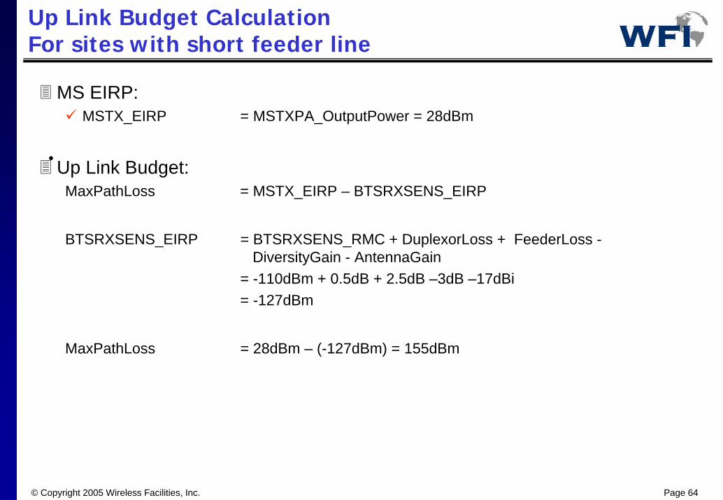
Up Link Budget CalculationFor sites with short feeder line
MS EIRP:MSTX_EIRP = MSTXPA_OutputPower = 28dBm
Up Link Budget:MaxPathLoss = MSTX_EIRP – BTSRXSENS_EIRP
BTSRXSENS_EIRP = BTSRXSENS_RMC + DuplexorLoss + FeederLoss -DiversityGain - AntennaGain
= -110dBm + 0.5dB + 2.5dB –3dB –17dBi= -127dBm
MaxPathLoss = 28dBm – (-127dBm) = 155dBm
•
© Copyright 2005 Wireless Facilities, Inc. Page 65
Path Balancing
The limiting path is the uplink which provides the worst link budget (155dBm).
In order to balance the uplink and downlink paths,
The PA setting at the BTS should be set to 43dBm (38.2dBm at the RBS cabinet TX connector) to make the downlink budget about equal to the uplink budget.
© Copyright 2005 Wireless Facilities, Inc. Page 66
Down Link Budget CalculationFor sites with long feeder line
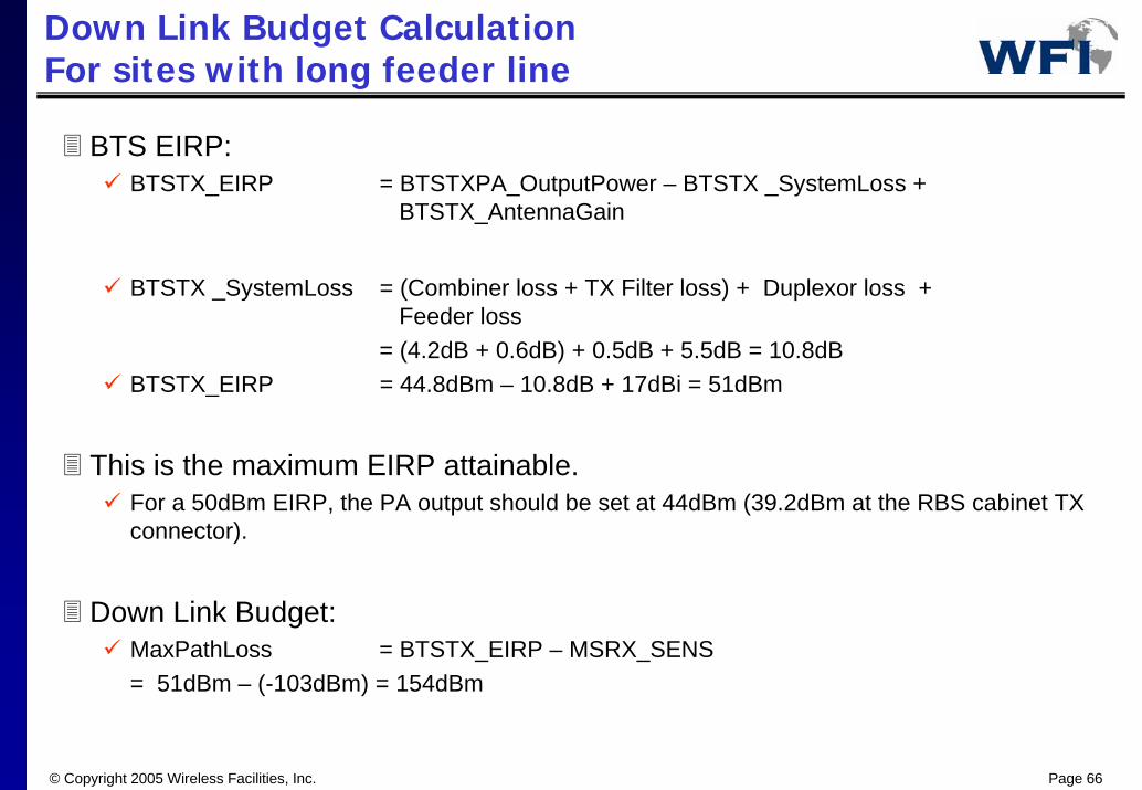
BTS EIRP:BTSTX_EIRP = BTSTXPA_OutputPower – BTSTX _SystemLoss +
BTSTX_AntennaGain
BTSTX _SystemLoss = (Combiner loss + TX Filter loss) + Duplexor loss + Feeder loss
= (4.2dB + 0.6dB) + 0.5dB + 5.5dB = 10.8dBBTSTX_EIRP = 44.8dBm – 10.8dB + 17dBi = 51dBm
This is the maximum EIRP attainable. For a 50dBm EIRP, the PA output should be set at 44dBm (39.2dBm at the RBS cabinet TX connector).
Down Link Budget:MaxPathLoss = BTSTX_EIRP – MSRX_SENS= 51dBm – (-103dBm) = 154dBm

© Copyright 2005 Wireless Facilities, Inc. Page 67
Up Link Budget CalculationFor sites with long feeder line
Up Link Budget:
MaxPathLoss = MSTX_EIRP – BTSRXSENS_EIRP
BTSRXSENS_EIRP = BTSRXSENS_RMC + DuplexorLoss + FeederLoss -DiversityGain - AntennaGain
= -110dBm + 0.5dB + 5.5dB – 3dB – 17dBi = -124dBm
MaxPathLoss = 28dBm – (-124dBm) = 152dBm
•
© Copyright 2005 Wireless Facilities, Inc. Page 68
Path Balancing
The limiting path is the uplink which provides the worst link budget (152dBm). In order to balance the uplink and downlink paths,
The PA setting at the BTS should be set to 43dBm (38.2dBm at the RBS cabinet TX connector) to make the downlink budget about equal to the uplink budget.
Reducing the BTS output power will affect the cell coverage radius.
Tower Mounted Amplifiers (TMA) can be used to improve the over all sensitivity of BTS.
© Copyright 2005 Wireless Facilities, Inc. Page 69
Noise and Interference limitation
Receiver minimum detectable signal power is limited by some unavoidable signals:
External - co-channel and adjacent channel interference,
Internal - thermal noise, due to motion of separate discrete electrons in wiring.
© Copyright 2005 Wireless Facilities, Inc. Page 70
Thermal Noise
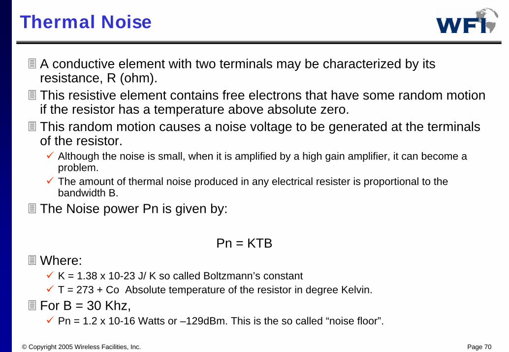
A conductive element with two terminals may be characterized by its resistance, R (ohm). This resistive element contains free electrons that have some random motion if the resistor has a temperature above absolute zero. This random motion causes a noise voltage to be generated at the terminals of the resistor.
Although the noise is small, when it is amplified by a high gain amplifier, it can become a problem. The amount of thermal noise produced in any electrical resister is proportional to the bandwidth B.
The Noise power Pn is given by:
Pn = KTBWhere:
K = 1.38 x 10⁻²³ J/ K so called Boltzmann’s constantT = 273 + Co Absolute temperature of the resistor in degree Kelvin.
For B = 30 Khz, Pn = 1.2 x 10⁻¹⁶ Watts or –129dBm. This is the so called “noise floor”.
© Copyright 2005 Wireless Facilities, Inc. Page 71
Noise Figure
To characterize the effectiveness of a device, a figure of merit is needed that compares the actual (noisy) device with an ideal device (no internal noise source).
A figure of merit, Noise Factor F, is the measure of the degradation of the signal to noise ratio due to the noise added in the device.
F = (S/N)i / (S/N)o,
Noise Figure NF = 10 Log10 F
© Copyright 2005 Wireless Facilities, Inc. Page 72
Noise Figure (cont’d)
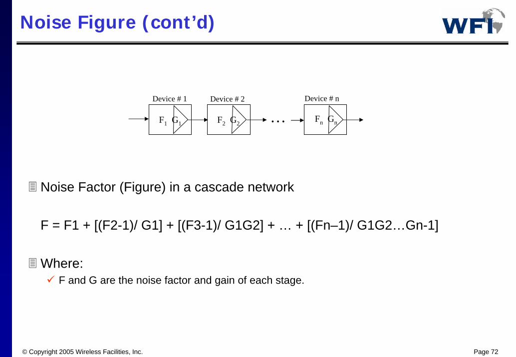
F1 G1 F2 G2 Fn Gn…Device # 1 Device # 2 Device # n
Noise Factor (Figure) in a cascade network
F = F1 + [(F2-1)/ G1] + [(F3-1)/ G1G2] + … + [(Fn–1)/ G1G2…Gn-1]
Where:F and G are the noise factor and gain of each stage.
© Copyright 2005 Wireless Facilities, Inc. Page 73
Noise Figure (cont’d)
The preceding equation for Noise Figure in a cascade network states that if the power gain of the first stage is large, the overall noise figure of the network will be essentially that of the first stage. Thus, in a receiving system design it is important that the first stage to have a low noise figure and a large gain so that the noise figure of the overall system will be as small as possible. That is why in a BTS design the TMA (low noise/ high gain amplifier) is placed next to the antenna on top of the tower.
Receiver Sensitivity:The available input signal level, Si, for a given output signal to noise ratio (S/N)o is referred to as the receiver sensitivity.
Si = F (KTB) (S/N)o
© Copyright 2005 Wireless Facilities, Inc. Page 74
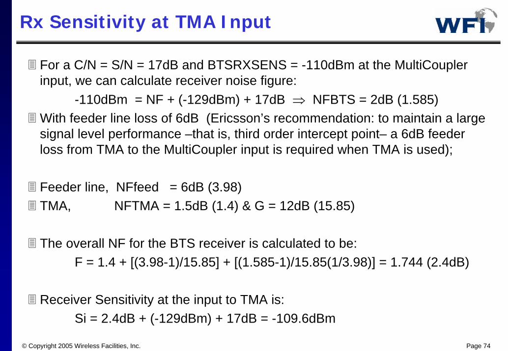
Rx Sensitivity at TMA Input
For a C/N = S/N = 17dB and BTSRXSENS = -110dBm at the MultiCouplerinput, we can calculate receiver noise figure:
-110dBm = NF + (-129dBm) + 17dB ⇒ NFBTS = 2dB (1.585)With feeder line loss of 6dB (Ericsson’s recommendation: to maintain a large signal level performance –that is, third order intercept point– a 6dB feeder loss from TMA to the MultiCoupler input is required when TMA is used);
Feeder line, NFfeed = 6dB (3.98) TMA, NFTMA = 1.5dB (1.4) & G = 12dB (15.85)
The overall NF for the BTS receiver is calculated to be:F = 1.4 + [(3.98-1)/15.85] + [(1.585-1)/15.85(1/3.98)] = 1.744 (2.4dB)
Receiver Sensitivity at the input to TMA is:Si = 2.4dB + (-129dBm) + 17dB = -109.6dBm

© Copyright 2005 Wireless Facilities, Inc. Page 75
Up Link Budget With TMA
Up Link Budget:
MaxPathLoss = MSTX_EIRP – BTSRXSENS_EIRP
BTSRXSENS_EIRP = BTSRXSENS_TMA + TopJumperLoss – DiversityGain- AntennaGain= -109.6dBm + 0.2dB –3dB –17dBi= -129.4dBm
MaxPathLoss = 28dBm – (-129.4dBm) = 157.4dBm
With the introduction of TMA to the system, the uplink budget is improved by about 6dB, and the uplink is no longer the limiting path
© Copyright 2005 Wireless Facilities, Inc. Page 76
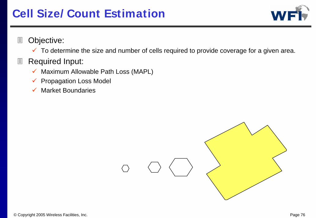
Cell Size/Count Estimation
Objective:To determine the size and number of cells required to provide coverage for a given area.
Required Input:Maximum Allowable Path Loss (MAPL)Propagation Loss ModelMarket Boundaries

© Copyright 2005 Wireless Facilities, Inc. Page 77
Cell Size/Count Estimation
Link Budget Analysis
Max Allowable Path Loss
Cell Radius Estimate
Cell Count Estimate
Path Loss Model
Field Tests
Market Boundaries
© Copyright 2005 Wireless Facilities, Inc. Page 78
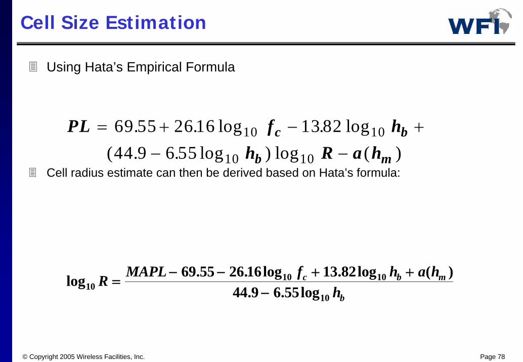
Cell Size Estimation
PL f hh R a h
c b
b m
= + − +− −
69 55 26 16 13 8244 9 6 55
10 10
10 10
. . log . log( . . log ) log ( )
log . . log . log ( ). . log10
10 10
10
69 55 26 16 13 8244 9 6 55
R MAPL f h a hh
c b m
b=
− − + +−
Using Hata’s Empirical Formula
Cell radius estimate can then be derived based on Hata’s formula:

© Copyright 2005 Wireless Facilities, Inc. Page 79
Cell Count EstimationCell Count Estimation
© Copyright 2005 Wireless Facilities, Inc. Page 80
Frequency Planning
© Copyright 2005 Wireless Facilities, Inc. Page 81
Frequency Planning
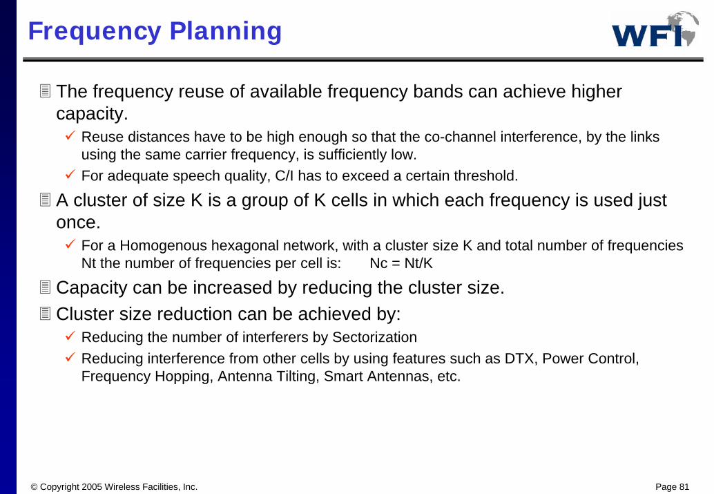
The frequency reuse of available frequency bands can achieve higher capacity.
Reuse distances have to be high enough so that the co-channel interference, by the links using the same carrier frequency, is sufficiently low.For adequate speech quality, C/I has to exceed a certain threshold.
A cluster of size K is a group of K cells in which each frequency is used just once.
For a Homogenous hexagonal network, with a cluster size K and total number of frequencies Nt the number of frequencies per cell is: Nc = Nt/K
Capacity can be increased by reducing the cluster size. Cluster size reduction can be achieved by:
Reducing the number of interferers by SectorizationReducing interference from other cells by using features such as DTX, Power Control, Frequency Hopping, Antenna Tilting, Smart Antennas, etc.
© Copyright 2005 Wireless Facilities, Inc. Page 82
Frequency Planning (cont’d)
The GSM specification states that the system should work satisfactorily down to C/I = 9dB.
However, it is recommended to use C/I = 12dB as a design figure to provide a useful margin.
It also states that a C/A = –9 dB should be the limit for acceptable adjacent channel interference.
With a 4/12 re-use pattern, the level of adjacent channel interference will be very difficult to reduce because so many of the channel groups are adjacent to each other. Therefore, it is recommended to use a C/A = –3 dB for a design target.
It is very efficient to use a combination of Frequency Hopping, Dynamic BTS and MS Power Control, and DTX.
The mutual interactions between these features provides a very powerful method to increase system performance. This yields that the system can utilize a tighter re-use pattern and thereby higher system capacity.
© Copyright 2005 Wireless Facilities, Inc. Page 83
Frequency Planning (cont’d)
A1A2
A3
B1B2
B3
D1D2
D3
C1C2
C3
A1A2
A3
B1B2
B3
D1D2
D3
C1C2
C3
A1A2
A3
B1B2
B3
D1D2
D3
C1C2
C3A1A2
A3
B1B2
B3
D1D2
D3
C1C2
C3
A1A2
A3
B1B2
B3
D1D2
D3
C1C2
C3
A1A2
A3
B1B2
B3
D1D2
D3
C1C2
C3A1A2
A3
B1B2
B3
D1D2
D3
C1C2
C3
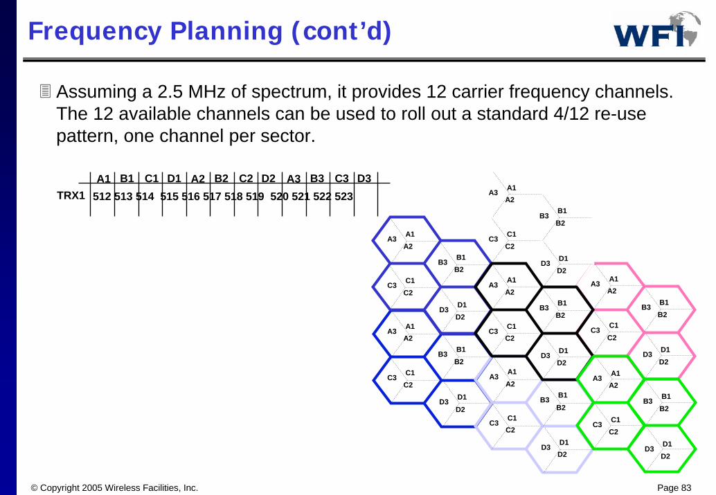
TRX1A1 B1 C1 D1 A2 B2 C2 D2 A3 B3 C3 D3
512 513 514 515 516 517 518 519 520 521 522 523
Assuming a 2.5 MHz of spectrum, it provides 12 carrier frequency channels. The 12 available channels can be used to roll out a standard 4/12 re-use pattern, one channel per sector.
© Copyright 2005 Wireless Facilities, Inc. Page 84
4/12 Re-use Pattern
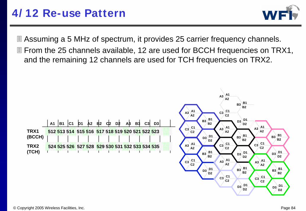
TRX1(BCCH)
512 513 514 515 516 517 518 519 520 521 522 523
A1 B1 C1 D1 A2 B2 C2 D2 A3 B3 C3 D3
524 525 526 527 528 529 530 531 532 533 534 535TRX2(TCH)
A1A2
A3
B1B2
B3
D1D2
D3
C1C2
C3
A1A2
A3
B1B2
B3
D1D2
D3
C1C2
C3
A1A2
A3
B1B2
B3
D1D2
D3
C1C2
C3A1A2
A3
B1B2
B3
D1D2
D3
C1C2
C3
A1A2
A3
B1B2
B3
D1D2
D3
C1C2
C3
A1A2
A3
B1B2
B3
D1D2
D3
C1C2
C3 A1A2
A3
B1B2
B3
D1D2
D3
C1C2
C3
Assuming a 5 MHz of spectrum, it provides 25 carrier frequency channels. From the 25 channels available, 12 are used for BCCH frequencies on TRX1, and the remaining 12 channels are used for TCH frequencies on TRX2.

© Copyright 2005 Wireless Facilities, Inc. Page 85
Multiple Re-use Pattern
TRX1(c0 filler)
512 513 514 515 516 517 518 519 520 521 522 523
A1 B1 C1 D1 A2 B2 C2 D2 A3 B3 C3 D3
TRX2TRX3(TCH)
524 525 526 527 528 529 530 531 532533 534 535
a1 b1 c1 a2 b2 c2 a3 b3 c3
A1A2
A3
B1B2
B3
D1D2
D3
C1C2
C3
A1A2
A3
B1B2
B3
D1D2
D3
C1C2
C3
A1A2
A3
B1B2
B3
D1D2
D3
C1C2
C3
A1A2
A3
B1B2
B3
D1D2
D3
C1C2
C3
A1A2
A3
B1B2
B3
D1D2
D3
C1C2
C3
A1A2
A3
B1B2
B3
D1D2
D3
C1C2
C3 A1A2
A3
B1B2
B3
D1D2
D3
C1C2
C3
b1
B2b3
c1
c2
c3
a1
a2
a3
b1
B2b3
c1
c2
c3
a1
a2
a3b1
B2b3
c1
c2
c3
a1
a2
a3b1
B2b3
c1
c2
c3
a1
a2
a3
b1
B2b3
c1
c2
c3
a1
a2
a3
b1
B2b3
c1
c2
c3
a1
a2
a3
b1
B2b3
c1
c2
c3
a1
a2
a3
From the 25 channels available, 12 are used for a standard 4/12 re-use pattern for BCCH frequencies. The remaining 12 channels can be assigned to a 3/9 re-use pattern. Employing Synthesizer (RF) hopping with BCCH frequency included, TRX1 operates only as c0 filler, and TRX2 will be hopping on all available frequencies.

© Copyright 2005 Wireless Facilities, Inc. Page 86
1/3 Fractional Re-use Pattern
For a small bandwidth allocation, the fractional 1/3 re-use provides a higher number of frequencies to hop on compared to standard 3/9 re-use pattern.
This provides a better service quality since it takes full advantage of frequency hopping. The gain in quality can be turned into a gain in capacity since the load can be increase by the addition of a TRX.
In a fractional re-use, the available spectrum is divided into two sets:A first set corresponding to the BCCH carrier frequencies re-used according to a 4/12 re-use pattern.A second set for the other frequencies re-used according to the fractional 1/3 re-use pattern.

© Copyright 2005 Wireless Facilities, Inc. Page 87
1/3 Fractional Re-use Pattern (cont.)
A1A2
A3
B1B2
B3
D1D2
D3
C1C2
C3
A1A2
A3
B1B2
B3
D1D2
D3
C1C2
C3
A1A2
A3
B1B2
B3
D1D2
D3
C1C2
C3
A1A2
A3
B1B2
B3
D1D2
D3
C1C2
C3
A1A2
A3
B1B2
B3
D1D2
D3
C1C2
C3
A1A2
A3
B1B2
B3
D1D2
D3
C1C2
C3 A1A2
A3
B1B2
B3
D1D2
D3
C1C2
C3
b1
B2b3
c1
c2
c3
a1
a2
a3
b1
B2b3
c1
c2
c3
a1
a2
a3b1
B2b3
c1
c2
c3
a1
a2
a3b1
B2b3
c1
c2
c3
a1
a2
a3
b1
B2b3
c1
c2
c3
a1
a2
a3
b1
B2b3
c1
c2
c3
a1
a2
a3
b1
B2b3
c1
c2
c3
a1
a2
a3
TRX1(c0 filler)
512 513 514 515 516 517 518 519 520 521 522 523A1 B1 C1 D1 A2 B2 C2 D2 A3 B3 C3 D3
TRX2TRX3(TCH)
a1 b1 c1
524 525 526527 528 529530 531 532533 534 535
Assuming a 5 MHz of spectrum, it provides 25 frequency channels.From the 25 channels available, 12 are used for a standard 4/12 re-use pattern for BCCH frequencies. The other 12 are assigned to a 1/3 fractional re-use pattern for TCH frequencies. The BCCH frequency should not be part of the hopping frequencies set for the fractional re-use.
© Copyright 2005 Wireless Facilities, Inc. Page 88
Traffic Capacity Analysis

© Copyright 2005 Wireless Facilities, Inc. Page 89
Traffic Capacity Requirement
Depending on the subscriber growth forecast, traffic analysis may show congestion soon after initial cell build out.
If Traffic analysis predicts high usage areas within the early days of system deployment, it may be necessary to reduce cell size and increase cell density in these areas to effectively handle offered traffic.
© Copyright 2005 Wireless Facilities, Inc. Page 90
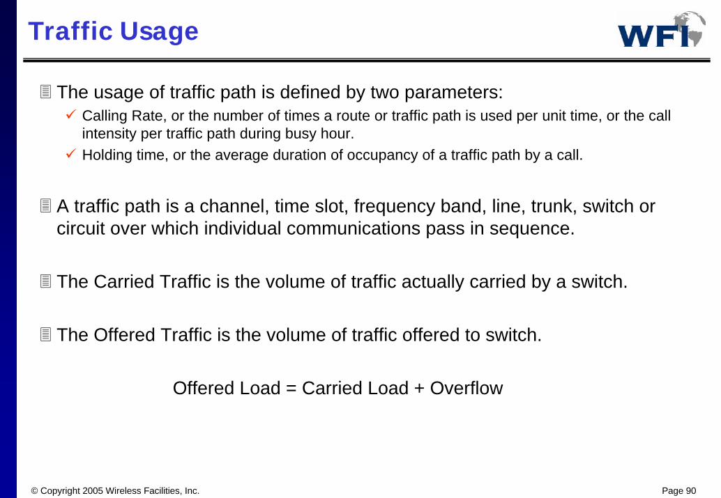
Traffic Usage
The usage of traffic path is defined by two parameters:Calling Rate, or the number of times a route or traffic path is used per unit time, or the call intensity per traffic path during busy hour.Holding time, or the average duration of occupancy of a traffic path by a call.
A traffic path is a channel, time slot, frequency band, line, trunk, switch or circuit over which individual communications pass in sequence.
The Carried Traffic is the volume of traffic actually carried by a switch.
The Offered Traffic is the volume of traffic offered to switch.
Offered Load = Carried Load + Overflow
© Copyright 2005 Wireless Facilities, Inc. Page 91
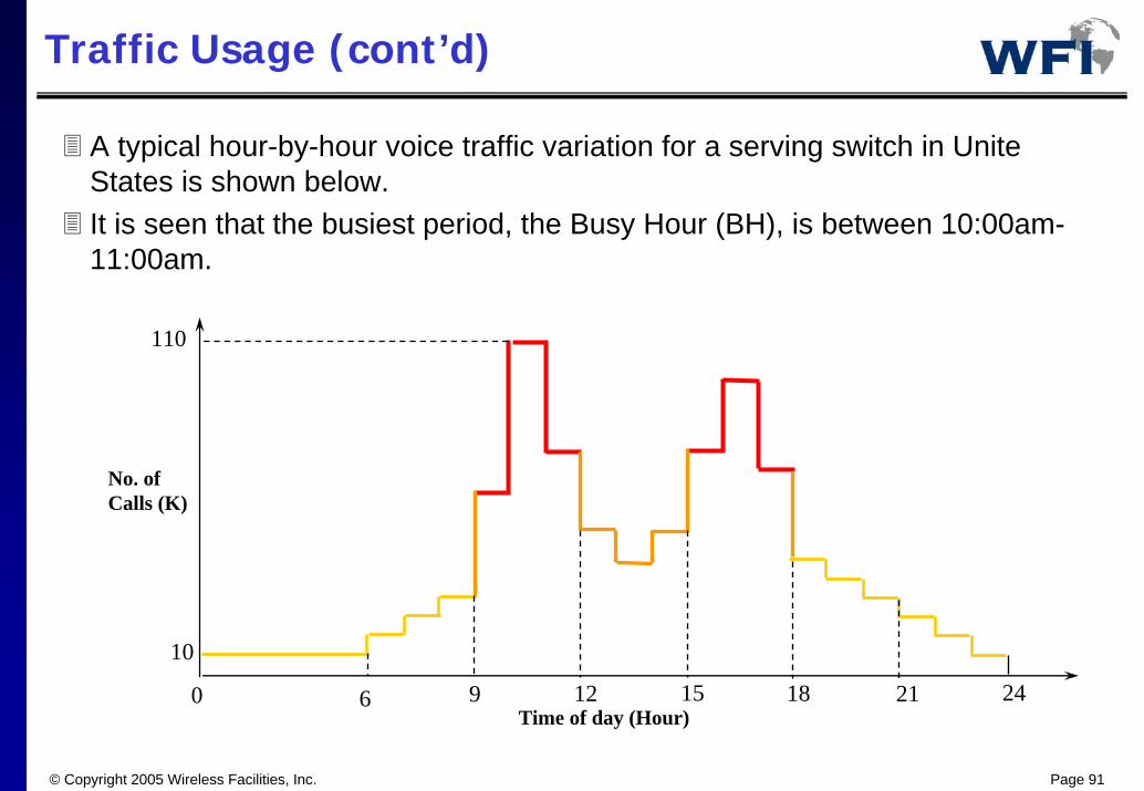
Traffic Usage (cont’d)
A typical hour-by-hour voice traffic variation for a serving switch in Unite States is shown below.It is seen that the busiest period, the Busy Hour (BH), is between 10:00am-11:00am.
0 6 129 15 18 21 24
110
10
Time of day (Hour)
No. ofCalls (K)

© Copyright 2005 Wireless Facilities, Inc. Page 92
Traffic Usage (cont’d)
The Busy Hour (BH) is defined as the time-consistent hour span of time (not necessarily a clock hour) that has the highest average traffic load for the business day throughout the business season.
The Peak Hour is defined as the clock hour with highest traffic load for a single day.
Since the traffic also varies from month to month, the Average Busy Season (ABS) is defined as the three months (not necessarily consecutive) with the highest average BH traffic load per access line.
Phone systems are not engineered for maximum peak loads, but for typical BH loads.
The blocking probability is defined as the average ratio of blocked calls to total calls and is referred to as the Grade of Service (GoS).
© Copyright 2005 Wireless Facilities, Inc. Page 93
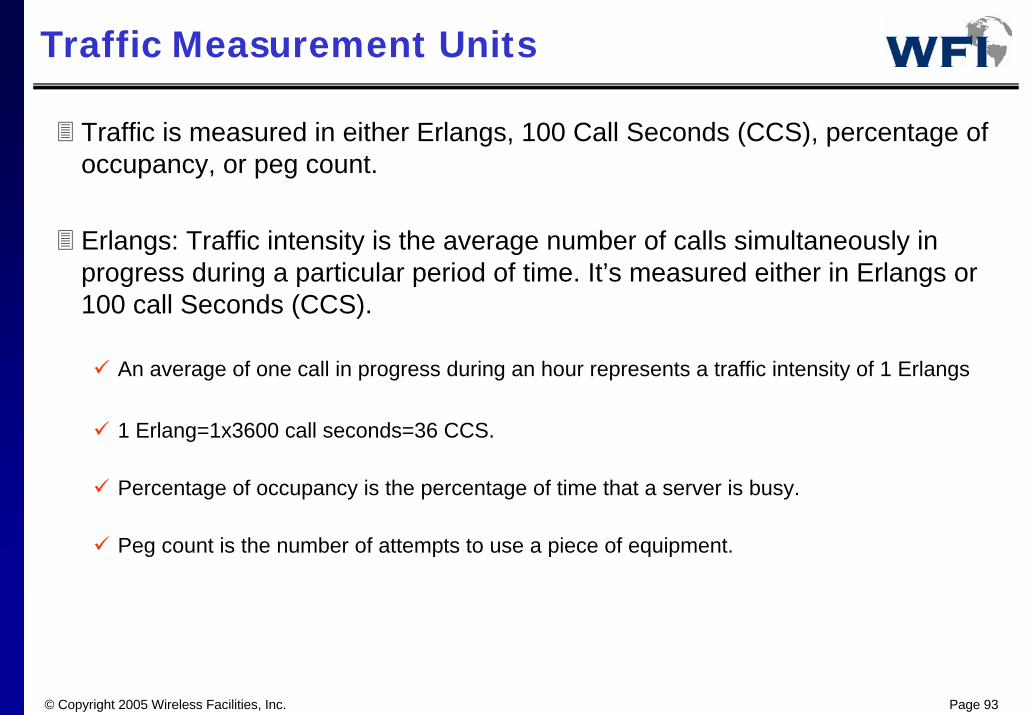
Traffic Measurement Units
Traffic is measured in either Erlangs, 100 Call Seconds (CCS), percentage of occupancy, or peg count.
Erlangs: Traffic intensity is the average number of calls simultaneously in progress during a particular period of time. It’s measured either in Erlangs or 100 call Seconds (CCS).
An average of one call in progress during an hour represents a traffic intensity of 1 Erlangs
1 Erlang=1x3600 call seconds=36 CCS.
Percentage of occupancy is the percentage of time that a server is busy.
Peg count is the number of attempts to use a piece of equipment.
© Copyright 2005 Wireless Facilities, Inc. Page 94
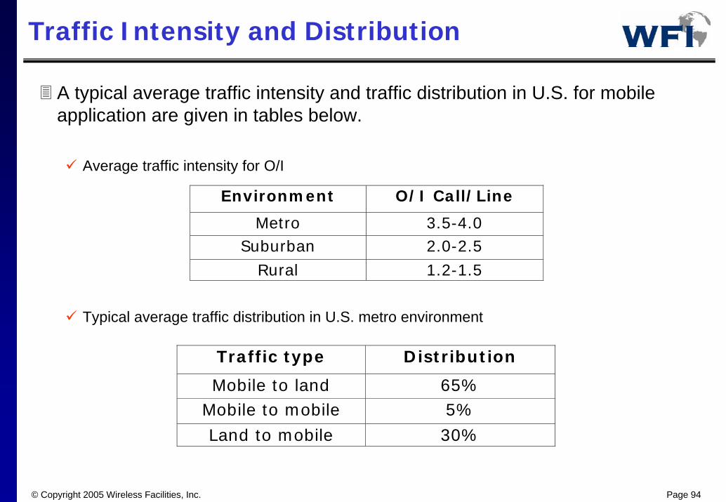
Traffic Intensity and Distribution
A typical average traffic intensity and traffic distribution in U.S. for mobile application are given in tables below.
Average traffic intensity for O/I
Typical average traffic distribution in U.S. metro environment
Environment O/I Call/Line
Metro 3.5-4.0Suburban 2.0-2.5
Rural 1.2-1.5
Traffic type Distribution
Mobile to land 65%Mobile to mobile 5%Land to mobile 30%
© Copyright 2005 Wireless Facilities, Inc. Page 95
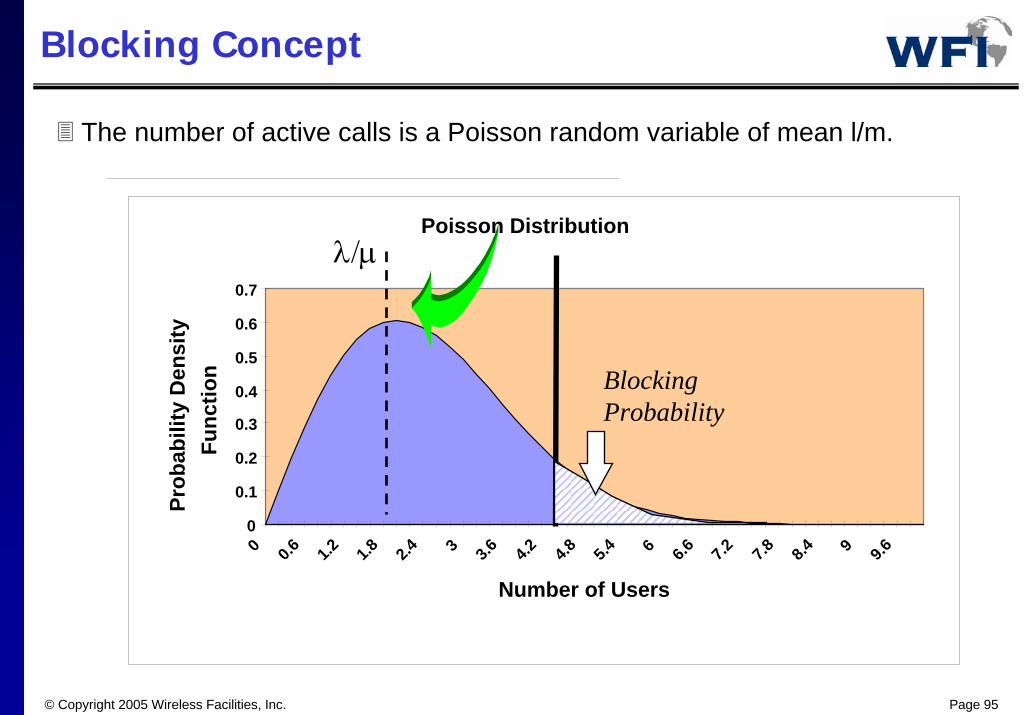
Blocking Concept
The number of active calls is a Poisson random variable of mean l/m.
0.2 0.099501 20.4 0.196040.6 0.2867990.8 0.369247
1 0.4412481.2 0.5011621.4 0.5478931.6 0.5809191.8 0.600279
2 0.6065312.2 0.6006822.4 0.5841032.6 0.5584252.8 0.525436
3 0.4869790.44486
0.4007680.3562180.3125010.2706710.231526
4.4 0.195628
Poisson Distribution
0
0.1
0.2
0.3
0.4
0.5
0.6
0.7
0 0.6 1.2 1.8 2.4 3 3.6 4.2 4.8 5.4 6 6.6 7.2 7.8 8.4 9 9.6
Number of Users
Prob
abili
ty D
ensi
ty
Func
tion Blocking
Probability
λ/µ
© Copyright 2005 Wireless Facilities, Inc. Page 96
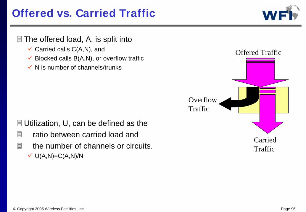
Offered vs. Carried Traffic
Offered Traffic
CarriedTraffic
OverflowTraffic
The offered load, A, is split intoCarried calls C(A,N), and Blocked calls B(A,N), or overflow trafficN is number of channels/trunks
Utilization, U, can be defined as theratio between carried load and the number of channels or circuits.U(A,N)=C(A,N)/N
© Copyright 2005 Wireless Facilities, Inc. Page 97
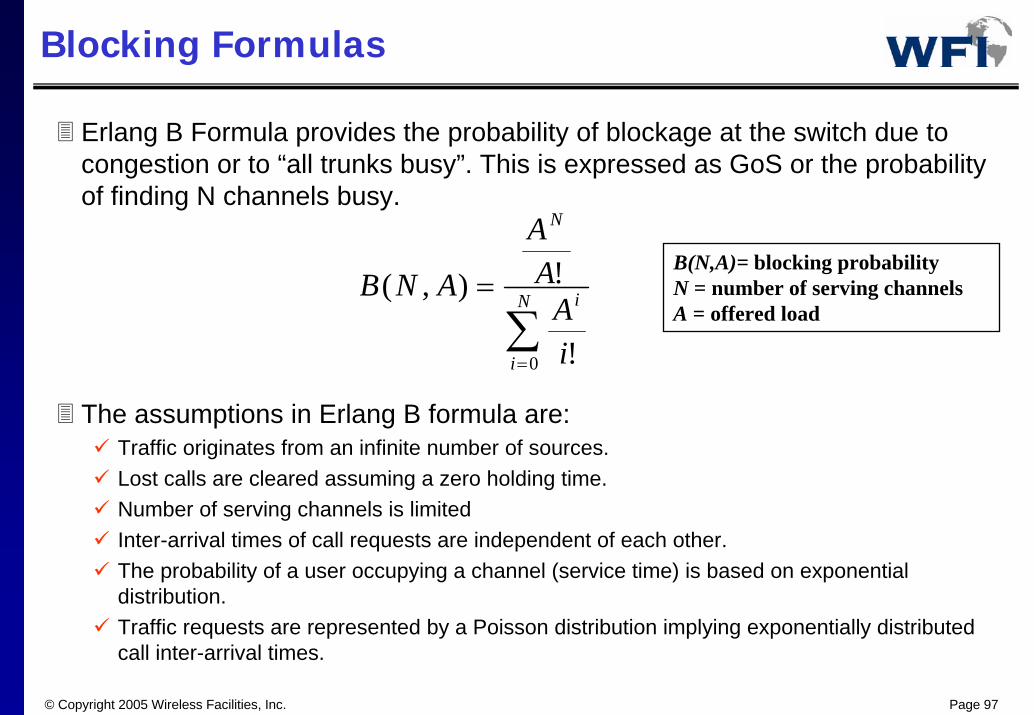
Blocking Formulas
Erlang B Formula provides the probability of blockage at the switch due to congestion or to “all trunks busy”. This is expressed as GoS or the probability of finding N channels busy.
The assumptions in Erlang B formula are:Traffic originates from an infinite number of sources.Lost calls are cleared assuming a zero holding time.Number of serving channels is limitedInter-arrival times of call requests are independent of each other.The probability of a user occupying a channel (service time) is based on exponential distribution.Traffic requests are represented by a Poisson distribution implying exponentially distributed call inter-arrival times.
∑=
= N
i
i
N
iA
AA
ANB
0 !
!),(B(N,A)= blocking probabilityN = number of serving channelsA = offered load
© Copyright 2005 Wireless Facilities, Inc. Page 98
Blocking Formulas (cont’d)
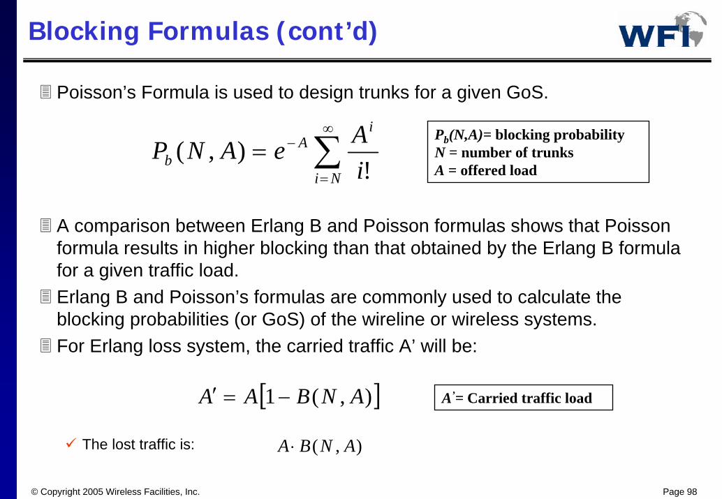
Poisson’s Formula is used to design trunks for a given GoS.
A comparison between Erlang B and Poisson formulas shows that Poisson formula results in higher blocking than that obtained by the Erlang B formula for a given traffic load.Erlang B and Poisson’s formulas are commonly used to calculate the blocking probabilities (or GoS) of the wireline or wireless systems. For Erlang loss system, the carried traffic A’ will be:
The lost traffic is:
∑∞
=
−=Ni
iA
b iAeANP!
),(Pb(N,A)= blocking probabilityN = number of trunksA = offered load
[ ]),(1 ANBAA −=′ A’= Carried traffic load
),( ANBA ⋅

© Copyright 2005 Wireless Facilities, Inc. Page 99
Blocking Formulas (cont’d)
Erlang C Formula assumes that a queue is formed to hold all requested calls that can not be served immediately. This means that blocked customers are delayed.
The assumptions in Erlang C formula are:Infinite sourcesPoisson inputLost calls delayedExponential holding timecalls served in order of arrival
∑−
= −+
−= 1
0 )1(!!
)1(!),( N
i
Ni
N
NANA
iA
NANA
ANCC(N,A)= blocking probabilityN = number of serving channelsA = offered load
© Copyright 2005 Wireless Facilities, Inc. Page 100
Blocking Formulas (cont’d)
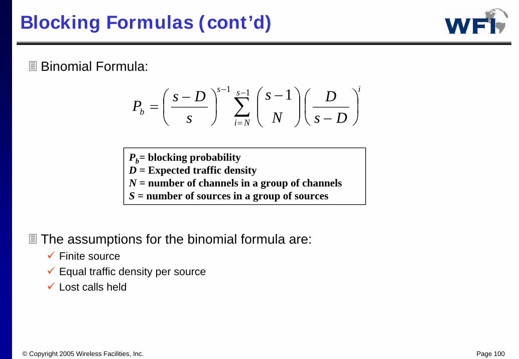
Binomial Formula:
The assumptions for the binomial formula are:Finite sourceEqual traffic density per sourceLost calls held
is
Ni
s
b DsD
Ns
sDsP ⎟
⎠⎞
⎜⎝⎛
−⎟⎟⎠
⎞⎜⎜⎝
⎛ −⎟⎠⎞
⎜⎝⎛ −
= ∑−
=
− 11 1
Pb= blocking probabilityD = Expected traffic densityN = number of channels in a group of channelsS = number of sources in a group of sources

© Copyright 2005 Wireless Facilities, Inc. Page 101
Grade of Service
The Grade of Service (GOS) is a measure of the ability of the user accessibility to a trunked system.
Given a specific number of channels available in a system, the GOS is used to define the desired performance of a wireless system by specifying the desired probability of a user obtaining a traffic channel.
GOS is typically given as the likelihood that a call is blocked.
A commonly used value for GOS (blocking probability) is 2%.

© Copyright 2005 Wireless Facilities, Inc. Page 102
Traffic Forecasting
PCS carriers will have to determine the characteristics of their penetration rate for potential customers.
A list of different categories and the demographic population break down can be as following example:
1) Vehicle Traffic along the roads
Demographic2) Income of people from the age of 15-34 making $15 – 35k (Demo. 1)3) Income of people from the age of 35-44 making $35 – 50k (Demo. 2)4) Income of people from the age of 35-54 making $50k+ (Demo. 3)

© Copyright 2005 Wireless Facilities, Inc. Page 103
Traffic Forecasting (cont’d)
The break down for years 1 – 5 of the penetration rates per category can be as following example:
Year1 Year2 Year3 Year4 Year51) Vehicle Traffic 0.2 0.6 0.9 1.3 1.652) Demo. 1 0.05 0.24 0.55 0.75 0.913) Demo. 2 0.05 0.25 0.55 0.75 0.924) Demo. 3 0.15 0.4 0.65 0.92 1.2Comb. pen. rate 0.45% 1.49% 2.65% 3.72% 4.68%
These demographic penetration rates can be applied to each census block group (using MapInfo) to determine the potential customer base for that census block.
The vehicle traffic count can be determined for each of the roads and then be spread over the appropriate census block group with the associated penetration rate.

© Copyright 2005 Wireless Facilities, Inc. Page 104
Traffic Forecasting (cont’d)
The number from the vehicle traffic count is then combined with the potential demographics user for each census block group.
From this number and the Erlang per subscriber number calculated before, an Erlang value is determined for each census block group based upon the above assumptions and is spread over the associated area.
The study then can be produced based on the coverage area of each potential sector with an Erlang captured and the associated RF channels and RF carriers required.
© Copyright 2005 Wireless Facilities, Inc. Page 105
Network Planning

© Copyright 2005 Wireless Facilities, Inc. Page 106
Two Types of Traffic
The traffic capacity of the wireline/wireless network can be categorized as: Voice/Data traffic (Erlang traffic).Control/Signaling traffic (events traffic).
The signaling traffic capacity calculation is based on occurrence of an event (i.e.: Call Attempt (CA)) and does not involve the duration of the call.The calculation of the voice traffic considers the call duration
The measurement of the voice traffic is based on Erlang B (blocked calls are not retried).
Calls begin Calls end
© Copyright 2005 Wireless Facilities, Inc. Page 107
Two Types of Traffic (cont’d)
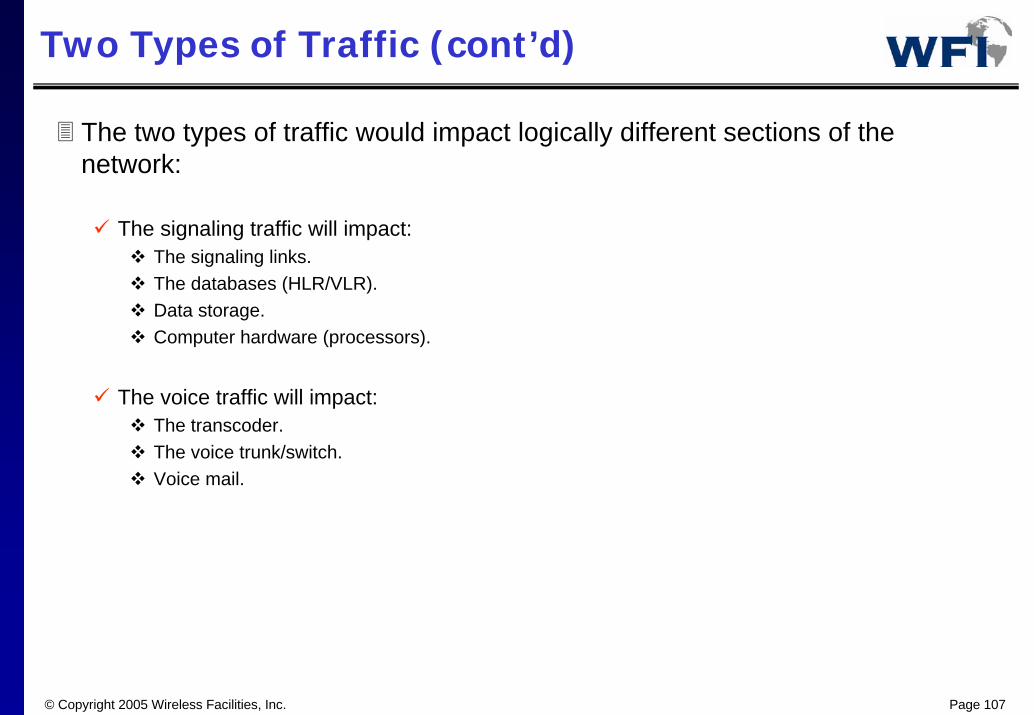
The two types of traffic would impact logically different sections of the network:
The signaling traffic will impact:The signaling links.The databases (HLR/VLR).Data storage.Computer hardware (processors).
The voice traffic will impact:The transcoder.The voice trunk/switch.Voice mail.

© Copyright 2005 Wireless Facilities, Inc. Page 108
Signaling Traffic Impact
The following events have major impact on the traffic calculations and processor utilization:
Call OriginationsCall TerminationsAuthenticationsHandoversLocation UpdatesIMSI Attach/Detach proceduresSMS ServicesData Services
© Copyright 2005 Wireless Facilities, Inc. Page 109
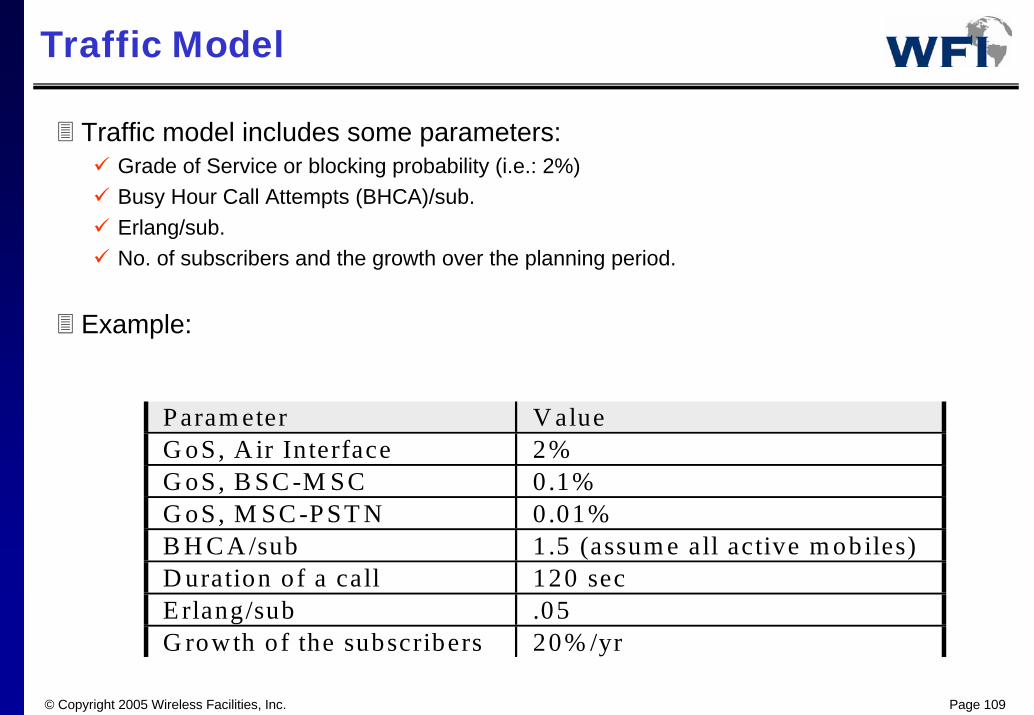
Traffic Model
Traffic model includes some parameters:Grade of Service or blocking probability (i.e.: 2%)Busy Hour Call Attempts (BHCA)/sub. Erlang/sub.No. of subscribers and the growth over the planning period.
Example:
P aram eter V alueG oS, A ir Interface 2%G oS, B SC -M SC 0.1%G oS, M SC -P ST N 0.01%B H C A /sub 1 .5 (assum e all active m obiles)D uration of a call 120 secE rlang/sub .05G rowth of the subscribers 20% /yr

© Copyright 2005 Wireless Facilities, Inc. Page 110
Call Mix Model
Call Mix Consists of: Mobile Origination Call (MOC) %Mobile Termination Call (MTC) %Mobile to Mobile (MTM) Attempts %Mobile Call Completion %
Example:
Parameter Value CompletionMOC(M-L) 60% %70MTM(M-M) 5% %40MTC(L-M) 35% %40
© Copyright 2005 Wireless Facilities, Inc. Page 111
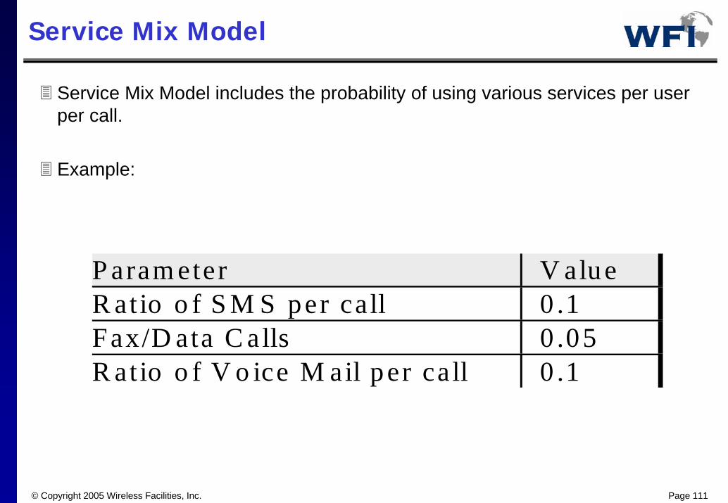
Service Mix Model
Service Mix Model includes the probability of using various services per user per call.
Example:
P aram eter V alueR atio o f S M S per call 0 .1Fax/D ata C alls 0 .05R atio o f V o ice M ail per call 0 .1
© Copyright 2005 Wireless Facilities, Inc. Page 112
Capacity Limits
The maximum network capacity (voice/signaling) is given for each network element.
Each element’s system limit is provided for future expansions (max number of processors)
For a voice sensitive element/link ( i.e., MSC, MC) maximum number of: ErlangsSubscribersTrunks
For a signaling sensitive element (HLR, VLR, SM_SC) maximum number of:Transactions/secData linksSubscribers

© Copyright 2005 Wireless Facilities, Inc. Page 113
NSS Elements’ Limits
The BSC limits are:Maximum no. of BTS that can be supported.Maximum no. of Call Attempt (CA).Maximum no. of voice ports it can support (I/O).Maximum no. of Signaling links that can be supported.
The MSC limits are:Maximum no. of BSC that can be supported .Maximum no. of Call Attempt (CA).Maximum no. of voice ports it can support (I/O).Maximum no. of Signaling links that can be supported.
© Copyright 2005 Wireless Facilities, Inc. Page 114
NSS Elements’ Limits (cont’d)
The VLR limits are:Maximum no. of subscribers (Size of the Memory).Maximum no. of transaction/sec processing on the VLR database.
The HLR limits are:Maximum no. of subscribers (Size of Memory).Maximum no. of Signaling links that can be supported.Maximum no. of transaction/sec processing on the HLR database.

© Copyright 2005 Wireless Facilities, Inc. Page 115
Joint Radio & Traffic Design
In principle radio coverage and traffic distribution are to be considered jointly.
However, due to the inherent task complexity, the procedure calculates:First, a suitable radio coverage for the service area, Then, it verifies if that coverage can fulfill the cell capacity requirements deriving from the traffic forecasting.
These two very strictly dependent steps are iterated until a satisfactory solution is derived.
The factors conditioning the resulting cell layout come from either propagation or traffic constraints, depending on the most critical conditions.

© Copyright 2005 Wireless Facilities, Inc. Page 116
Traffic Analysis
As for the traffic modeling, the service area must be characterized based on subscribers' density and distribution.
Geographical maps or territorial databases are utilized to identify the main roads, inhabitant densities, and business areas.
Urban and geographical analysis can be integrated, when necessary, with data relevant to the fixed telecommunication users distribution.
Since the mobility attributes affect signaling network and distributed data base dimensioning significantly, they are also modeled in this step.

© Copyright 2005 Wireless Facilities, Inc. Page 117
Subscriber Forecast
Service Types and percentagesVoice.Short Messages.Fax.Later on: Data/Internet Transactions.....
Service StatisticsAverage Call Duration.Erlangs/Sub.Outgoing vs. Incoming Call Ratios.....
DemographicsService Penetration.Total Number of Subscribers.Distribution of Subscribers.
Mobility of subscribersHandoff Rates.Location Update Rate.
© Copyright 2005 Wireless Facilities, Inc. Page 118
Demographics Analysis
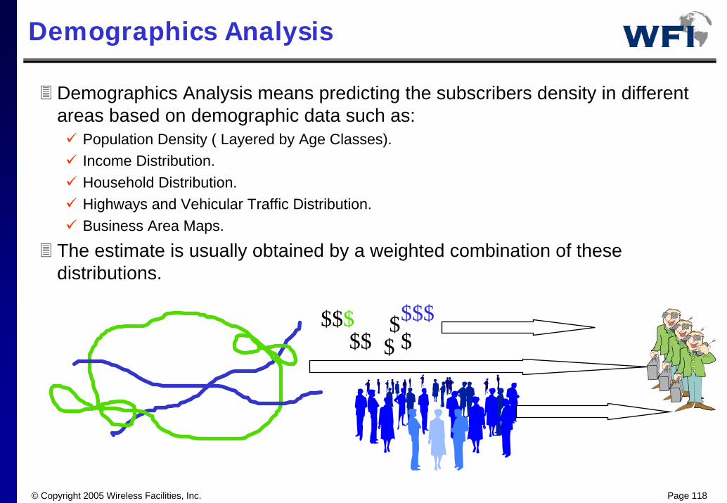
Demographics Analysis means predicting the subscribers density in different areas based on demographic data such as:
Population Density ( Layered by Age Classes).Income Distribution.Household Distribution.Highways and Vehicular Traffic Distribution.Business Area Maps.
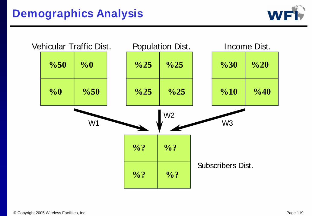
The estimate is usually obtained by a weighted combination of these distributions.
$$$$$
$$$$$$$
© Copyright 2005 Wireless Facilities, Inc. Page 119
Demographics Analysis
Vehicular Traffic Dist. Population Dist. Income Dist.
%50 %0
%50%0
%25 %25
%25%25
%30 %20
%40%10
%? %?
%?%?Subscribers Dist.
W1 W3W2

© Copyright 2005 Wireless Facilities, Inc. Page 120
Subs/Cell
Composite Coverage Design(Cell Footprints)
Subscriber Distribution Map

© Copyright 2005 Wireless Facilities, Inc. Page 121
Alternative Subscriber Forecast
Total Population,Service Penetration Factor
Total No. of Subscribers
LBA
MAPLPropagationModel
Market Area
Subscribers’ Density
# Subs/Cell
Cell Area
© Copyright 2005 Wireless Facilities, Inc. Page 122
Traffic Analysis for BTS
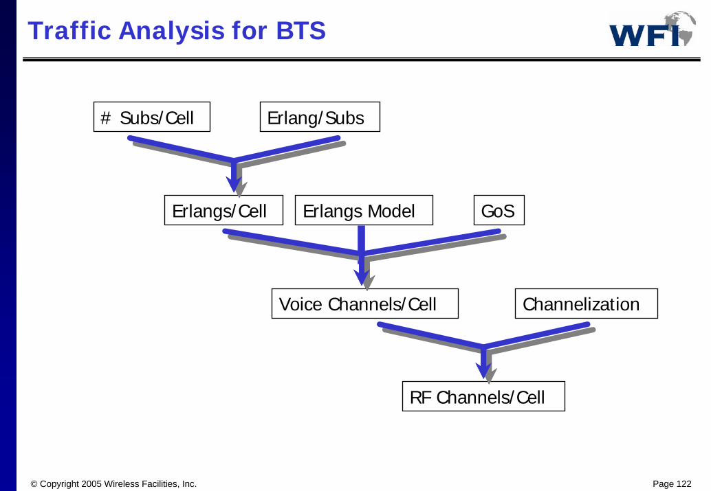
# Subs/Cell
Erlangs/Cell
Voice Channels/Cell
RF Channels/Cell
Erlang/Subs
Erlangs Model GoS
Channelization
© Copyright 2005 Wireless Facilities, Inc. Page 123
BTS Dimensioning
BTS
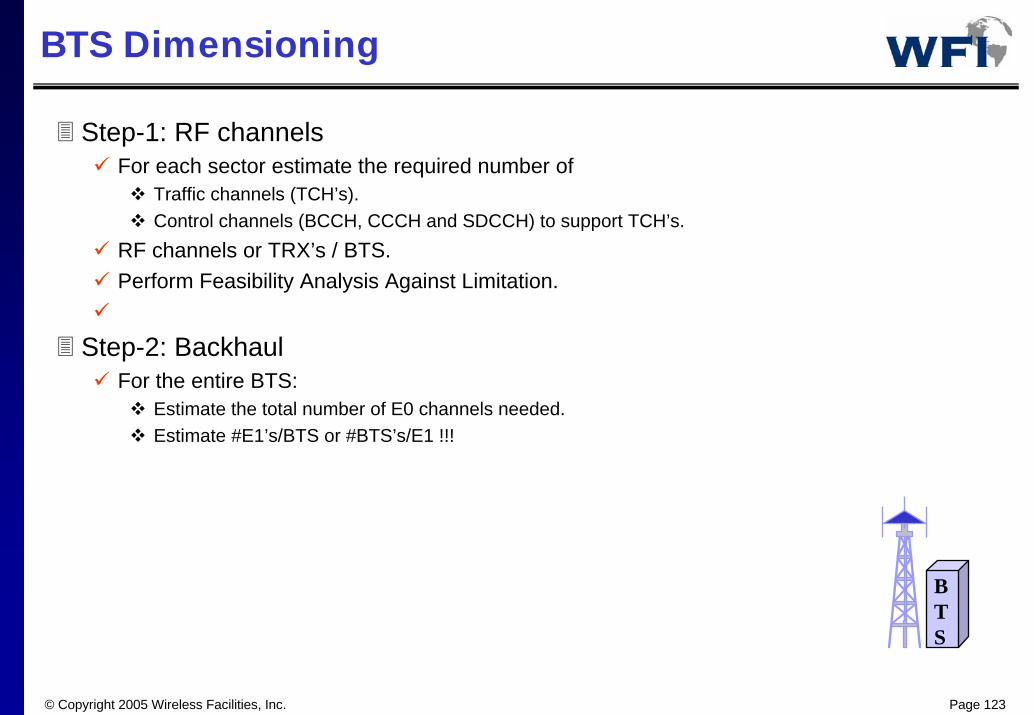
Step-1: RF channelsFor each sector estimate the required number of
Traffic channels (TCH’s).Control channels (BCCH, CCCH and SDCCH) to support TCH’s.
RF channels or TRX’s / BTS.Perform Feasibility Analysis Against Limitation.
Step-2: BackhaulFor the entire BTS:
Estimate the total number of E0 channels needed.Estimate #E1’s/BTS or #BTS’s/E1 !!!
© Copyright 2005 Wireless Facilities, Inc. Page 124
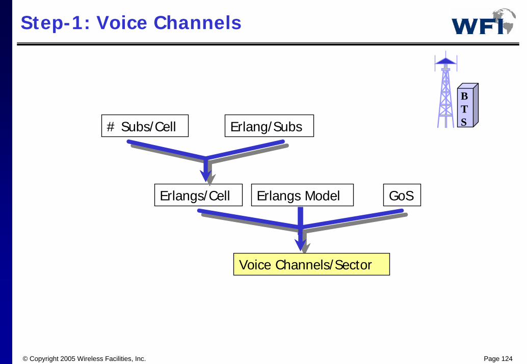
Step-1: Voice Channels
BTS# Subs/Cell
Erlangs/Cell
Erlang/Subs
Erlangs Model GoS
Voice Channels/Sector
© Copyright 2005 Wireless Facilities, Inc. Page 125
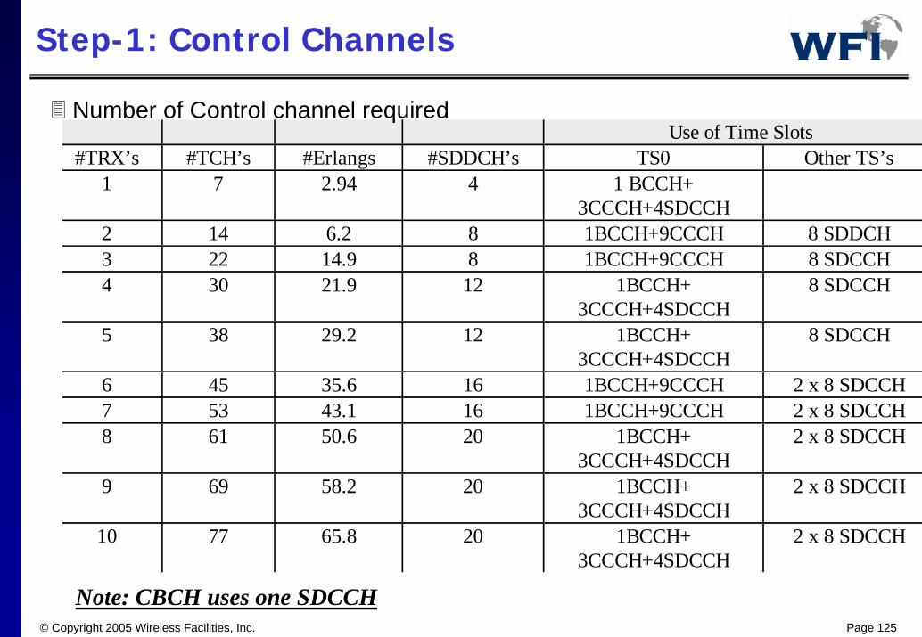
Step-1: Control Channels
Use of Time Slots#TRX’s #TCH’s #Erlangs #SDDCH’s TS0 Other TS’s
1 7 2.94 4 1 BCCH+3CCCH+4SDCCH
2 14 6.2 8 1BCCH+9CCCH 8 SDDCH3 22 14.9 8 1BCCH+9CCCH 8 SDCCH4 30 21.9 12 1BCCH+
3CCCH+4SDCCH8 SDCCH
5 38 29.2 12 1BCCH+3CCCH+4SDCCH
8 SDCCH
6 45 35.6 16 1BCCH+9CCCH 2 x 8 SDCCH7 53 43.1 16 1BCCH+9CCCH 2 x 8 SDCCH8 61 50.6 20 1BCCH+
3CCCH+4SDCCH2 x 8 SDCCH
9 69 58.2 20 1BCCH+3CCCH+4SDCCH
2 x 8 SDCCH
10 77 65.8 20 1BCCH+3CCCH+4SDCCH
2 x 8 SDCCH
Note: CBCH uses one SDCCH
Number of Control channel required
© Copyright 2005 Wireless Facilities, Inc. Page 126
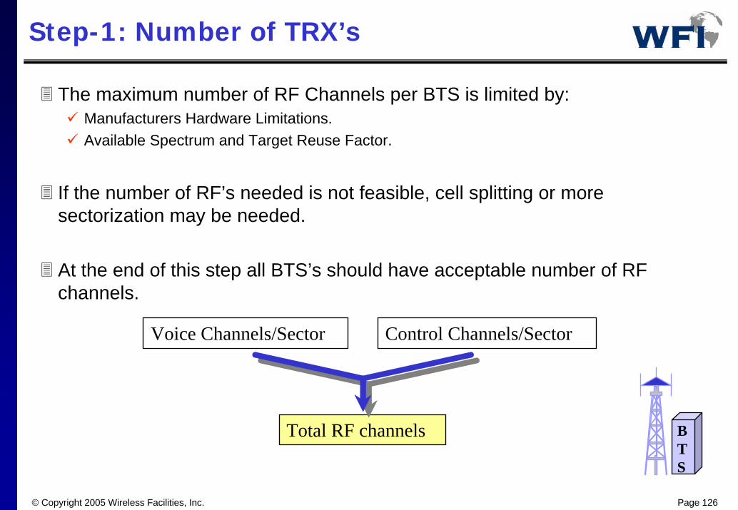
Step-1: Number of TRX’s
The maximum number of RF Channels per BTS is limited by:Manufacturers Hardware Limitations.Available Spectrum and Target Reuse Factor.
If the number of RF’s needed is not feasible, cell splitting or more sectorization may be needed.
At the end of this step all BTS’s should have acceptable number of RF channels.
Voice Channels/Sector
Total RF channels
Control Channels/Sector
BTS

© Copyright 2005 Wireless Facilities, Inc. Page 127
Step-2: Backhaul Consideration
Add the number of TCH’s needed on all sectors and calculate the numbers of E0’s needed.
If TRAU is at the BTS # E0 Channels = # TCH’s.
If TRAU is at BSC or MSC# E0 Channels = # TCH’s/4, rounded up????
Add One or two E0’s for Signaling/Control Information.
Estimate the number of E1’s neededTotal # E0 channels/30 = # E1 links
© Copyright 2005 Wireless Facilities, Inc. Page 128
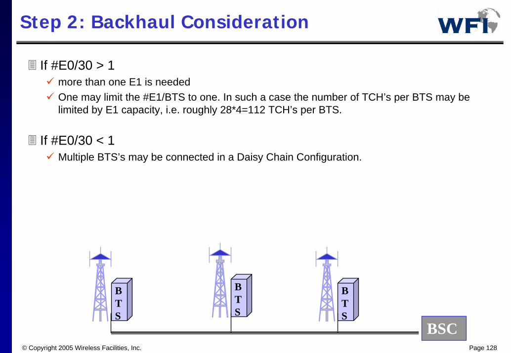
Step 2: Backhaul Consideration
If #E0/30 > 1more than one E1 is neededOne may limit the #E1/BTS to one. In such a case the number of TCH’s per BTS may be limited by E1 capacity, i.e. roughly 28*4=112 TCH’s per BTS.
If #E0/30 < 1Multiple BTS’s may be connected in a Daisy Chain Configuration.
BTS
BTS
BTS
BSC

© Copyright 2005 Wireless Facilities, Inc. Page 129
Example, GSM planning
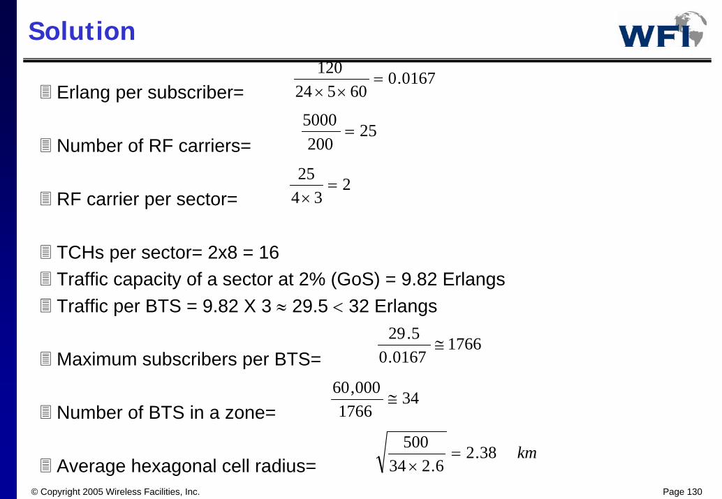
Problem Statement: Using the following data for a GSM system, calculate:1. Average busy hour traffic per subscriber2. Traffic capacity per cell3. Required number of BSs per zone and the hexagonal cell radius for the zone.System’s Data:
Subscriber usage per month=120 minutesDays per month=24Busy hours per day=5Allocated spectrum=5 MHzFrequency reuse plan=4/12RF channel width=200 KHz, full rateCapacity of a BTS=32 ErlangsSubscribers in the zone=60,000Area of the zone=500 km2
© Copyright 2005 Wireless Facilities, Inc. Page 130
Solution
Erlang per subscriber=
Number of RF carriers=
RF carrier per sector=
TCHs per sector= 2x8 = 16Traffic capacity of a sector at 2% (GoS) = 9.82 ErlangsTraffic per BTS = 9.82 X 3 ≈ 29.5 < 32 Erlangs
Maximum subscribers per BTS=
Number of BTS in a zone=
Average hexagonal cell radius=
0167.060524
120=
××
25200
5000=
234
25=
×
17660167.0
5.29≅
341766
000,60≅
km38.26.234
500=
×
© Copyright 2005 Wireless Facilities, Inc. Page 131
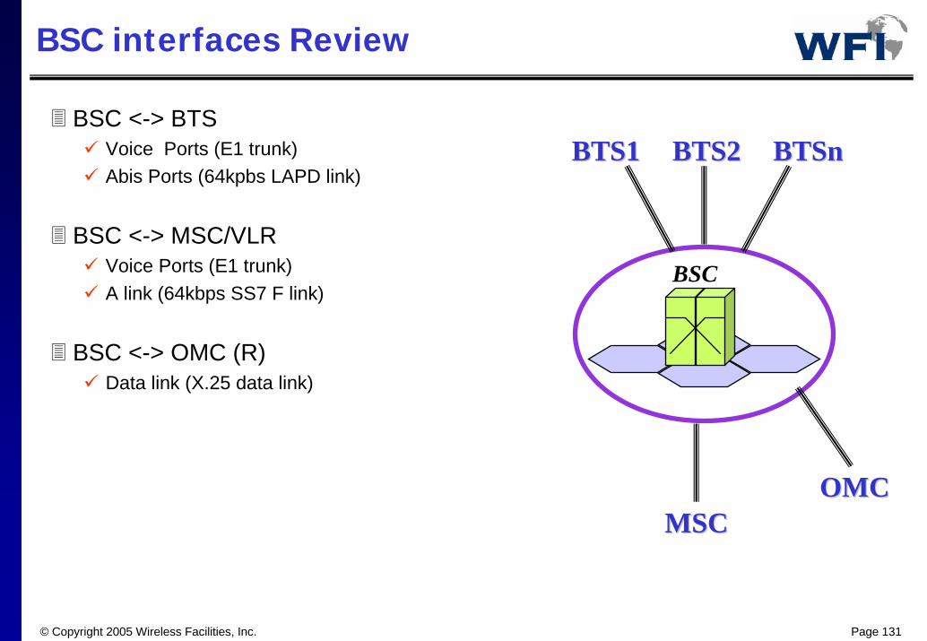
BSC interfaces Review
BSC <-> BTSVoice Ports (E1 trunk)Abis Ports (64kpbs LAPD link)
BSC <-> MSC/VLRVoice Ports (E1 trunk)A link (64kbps SS7 F link)
BSC <-> OMC (R)Data link (X.25 data link)
BSC
MSCMSC
BTS2BTS2
OMCOMC
BTSnBTSnBTS1BTS1
© Copyright 2005 Wireless Facilities, Inc. Page 132
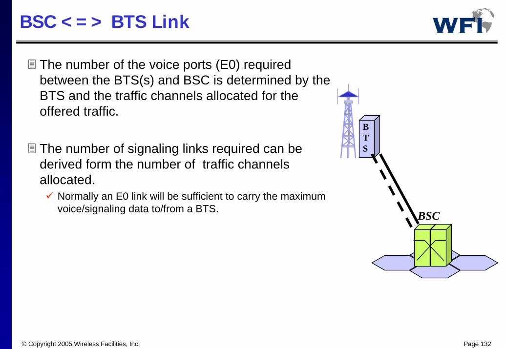
BSC <=> BTS Link
The number of the voice ports (E0) required between the BTS(s) and BSC is determined by the BTS and the traffic channels allocated for the offered traffic.
The number of signaling links required can be derived form the number of traffic channels allocated.
Normally an E0 link will be sufficient to carry the maximum voice/signaling data to/from a BTS.
BTS
BSC
© Copyright 2005 Wireless Facilities, Inc. Page 133
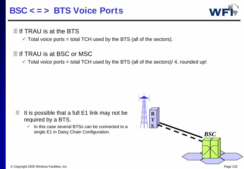
BSC <=> BTS Voice Ports
If TRAU is at the BTSTotal voice ports = total TCH used by the BTS (all of the sectors).
If TRAU is at BSC or MSCTotal voice ports = total TCH used by the BTS (all of the sectors)/ 4, rounded up!
BTS
BSC
It is possible that a full E1 link may not be required by a BTS.
In this case several BTSs can be connected to a single E1 in Daisy Chain Configuration.
© Copyright 2005 Wireless Facilities, Inc. Page 134
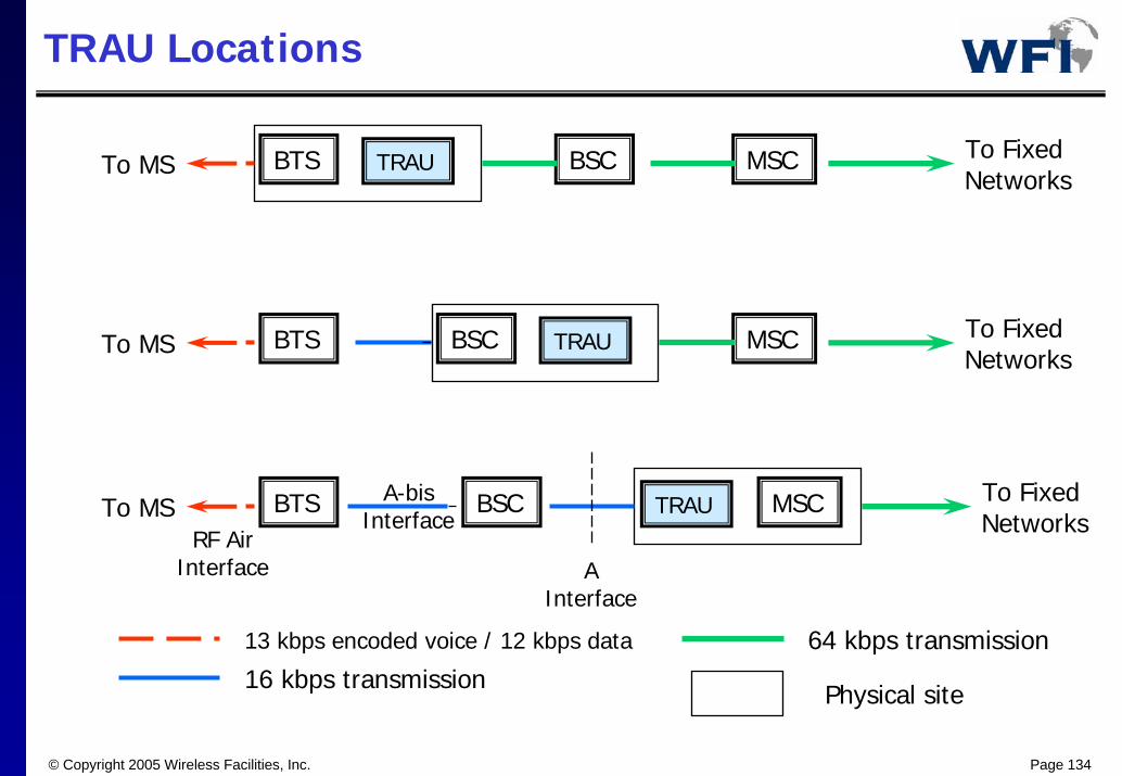
TRAU Locations
BTS TRAU BSC To Fixed Networks
MSCTo MS
BTS MSCBSC TRAU To Fixed NetworksTo MS
BTS MSC To Fixed NetworksTo MS BSC TRAU
AInterface
A-bisInterface
RF AirInterface
13 kbps encoded voice / 12 kbps data
16 kbps transmission64 kbps transmission
Physical site
© Copyright 2005 Wireless Facilities, Inc. Page 135
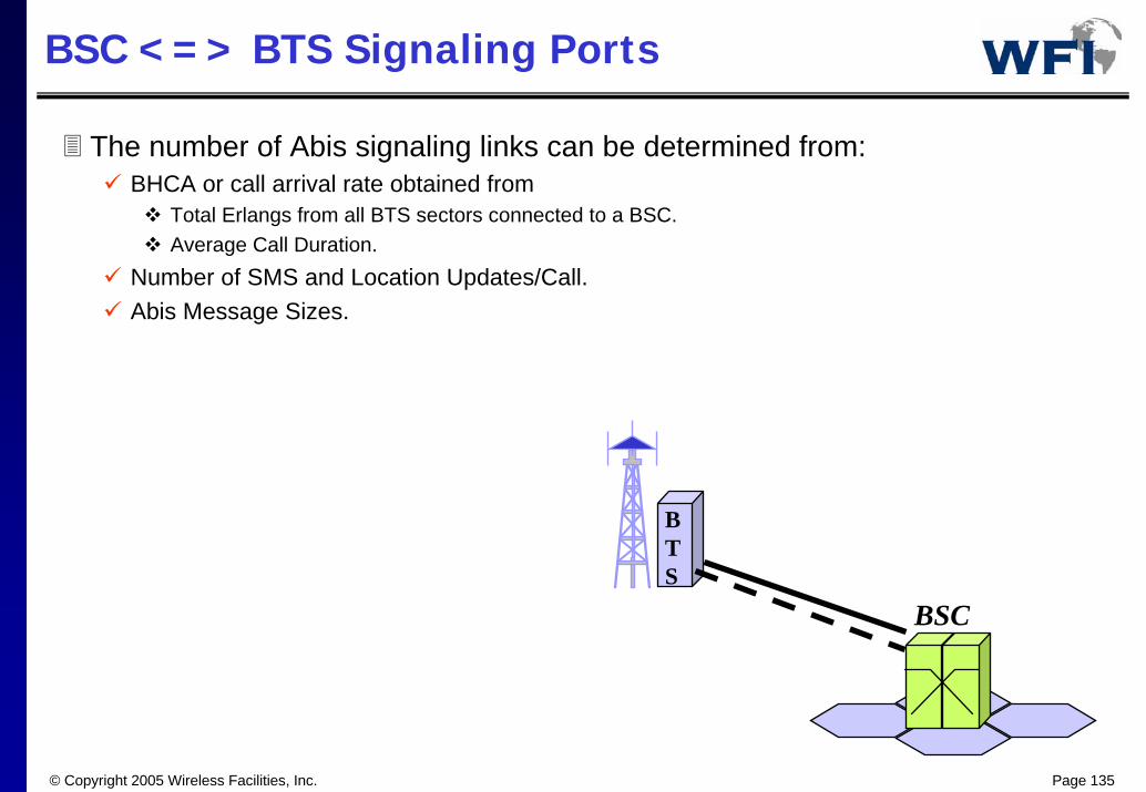
BSC <=> BTS Signaling Ports
The number of Abis signaling links can be determined from: BHCA or call arrival rate obtained from
Total Erlangs from all BTS sectors connected to a BSC.Average Call Duration.
Number of SMS and Location Updates/Call.Abis Message Sizes.
BTS
BSC
© Copyright 2005 Wireless Facilities, Inc. Page 136
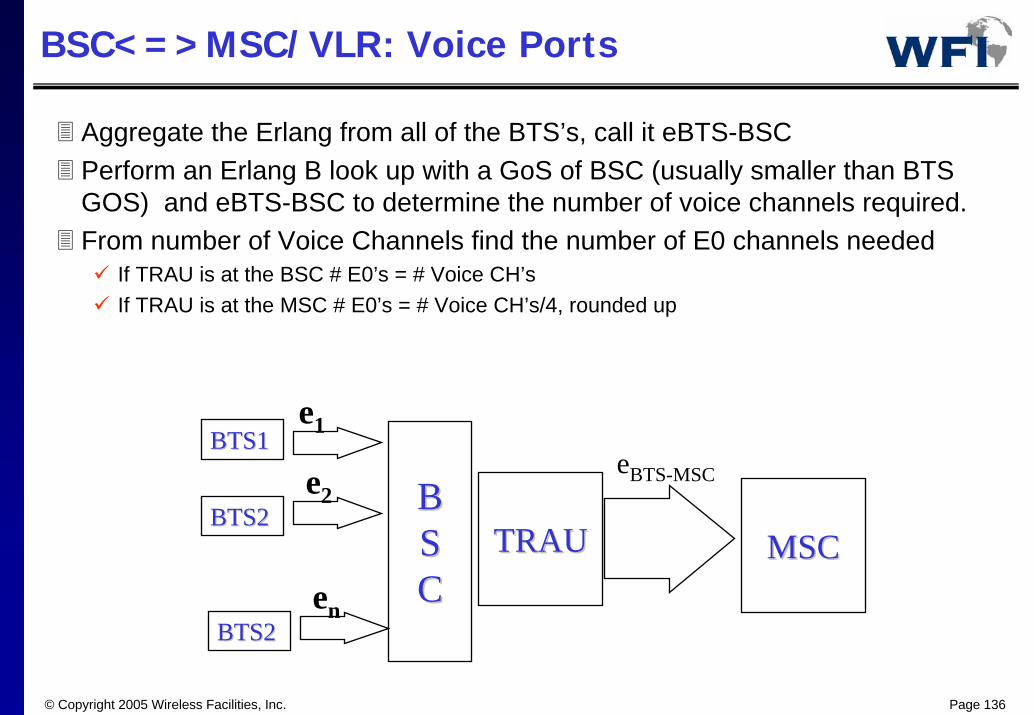
BSC<=>MSC/VLR: Voice Ports
Aggregate the Erlang from all of the BTS’s, call it eBTS-BSCPerform an Erlang B look up with a GoS of BSC (usually smaller than BTS GOS) and eBTS-BSC to determine the number of voice channels required.From number of Voice Channels find the number of E0 channels needed
If TRAU is at the BSC # E0’s = # Voice CH’sIf TRAU is at the MSC # E0’s = # Voice CH’s/4, rounded up
BTS1BTS1
BTS2BTS2 BBSSCC
TRAUTRAU
e1
e2
BTS2BTS2en
eBTS-MSC
MSCMSC
© Copyright 2005 Wireless Facilities, Inc. Page 137
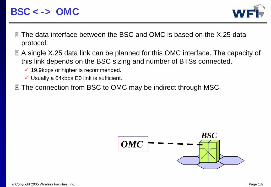
BSC <-> OMC
The data interface between the BSC and OMC is based on the X.25 data protocol.A single X.25 data link can be planned for this OMC interface. The capacity of this link depends on the BSC sizing and number of BTSs connected.
19.9kbps or higher is recommended.Usually a 64kbps E0 link is sufficient.
The connection from BSC to OMC may be indirect through MSC.
BSCOMC

© Copyright 2005 Wireless Facilities, Inc. Page 138
BSC Dimensioning (review)
The BSC capacity determines its ability to connect to, and process information received by, all the signaling links from the BTS, the MSC and the OMC. This capacity is usually expressed in terms of
Max_BTS: Total No of BTSs that can be supported/controlled,Max_TRX: Maximum number of TRXs in the connected BTSs,Max_CA: Maximum number of CA,Max_PORT: Total Number of Ports (input and output together).
BTS BSC
MSC/VLR
BTS
BTS
OMC
© Copyright 2005 Wireless Facilities, Inc. Page 139
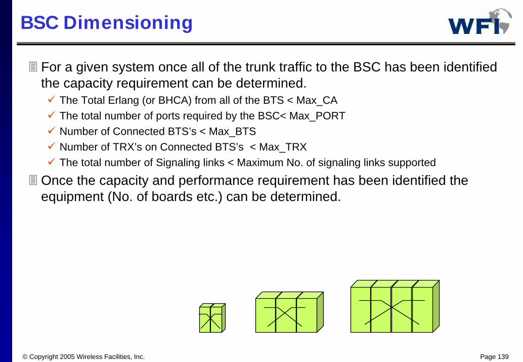
BSC Dimensioning
For a given system once all of the trunk traffic to the BSC has been identified the capacity requirement can be determined.
The Total Erlang (or BHCA) from all of the BTS < Max_CA The total number of ports required by the BSC< Max_PORTNumber of Connected BTS’s < Max_BTSNumber of TRX’s on Connected BTS’s < Max_TRXThe total number of Signaling links < Maximum No. of signaling links supported
Once the capacity and performance requirement has been identified the equipment (No. of boards etc.) can be determined.
© Copyright 2005 Wireless Facilities, Inc. Page 140
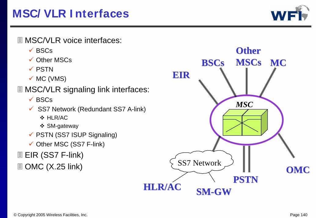
MSC/VLR Interfaces
MSC
PSTNPSTN
OtherOtherMSCsMSCs
OMCOMC
MCMCBSCsBSCs
HLR/ACHLR/AC SMSM--GWGW
SS7 Network
EIREIR
MSC/VLR voice interfaces:BSCsOther MSCsPSTNMC (VMS)
MSC/VLR signaling link interfaces:BSCsSS7 Network (Redundant SS7 A-link)
HLR/ACSM-gateway
PSTN (SS7 ISUP Signaling)Other MSC (SS7 F-link)
EIR (SS7 F-link)OMC (X.25 link)
© Copyright 2005 Wireless Facilities, Inc. Page 141
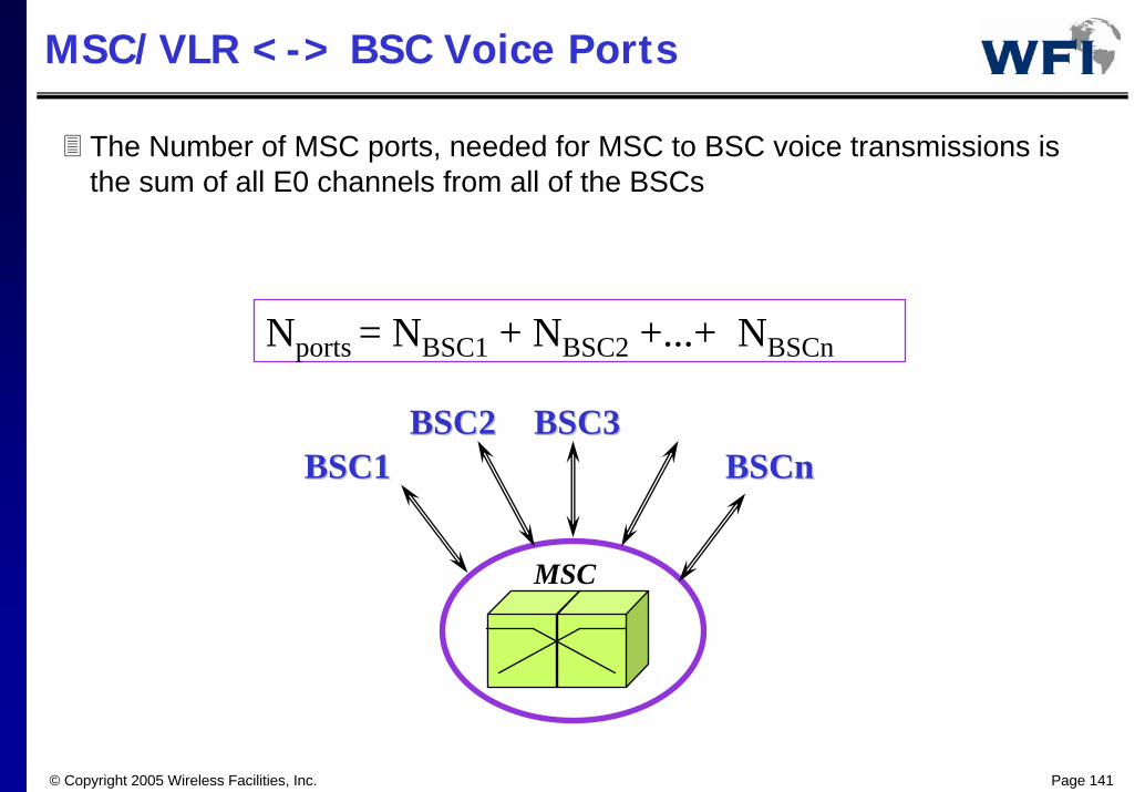
MSC/VLR <-> BSC Voice Ports
The Number of MSC ports, needed for MSC to BSC voice transmissions is the sum of all E0 channels from all of the BSCs
MSC
BSC3BSC3BSC2BSC2BSCnBSCnBSC1BSC1
Nports = NBSC1 + NBSC2 +...+ NBSCn
© Copyright 2005 Wireless Facilities, Inc. Page 142
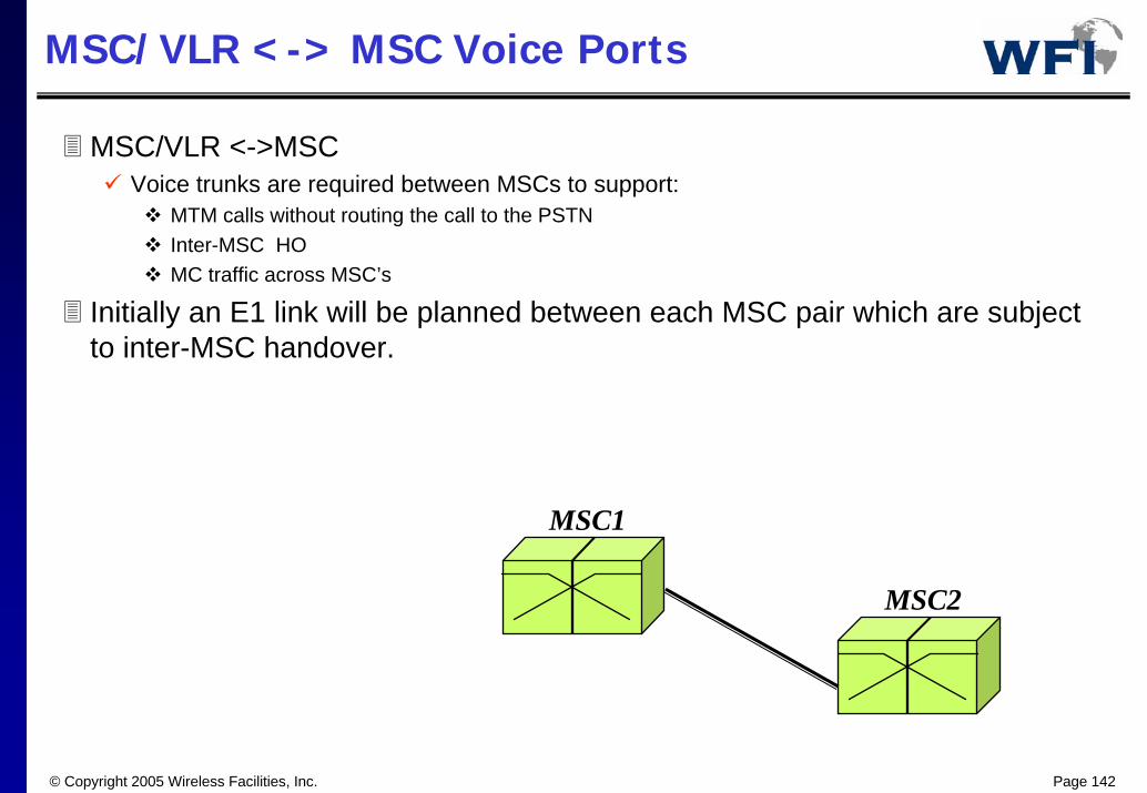
MSC/VLR <-> MSC Voice Ports
MSC/VLR <->MSCVoice trunks are required between MSCs to support:
MTM calls without routing the call to the PSTN Inter-MSC HOMC traffic across MSC’s
Initially an E1 link will be planned between each MSC pair which are subject to inter-MSC handover.
MSC1
MSC2
© Copyright 2005 Wireless Facilities, Inc. Page 143
MSC/VLR<->PSTN
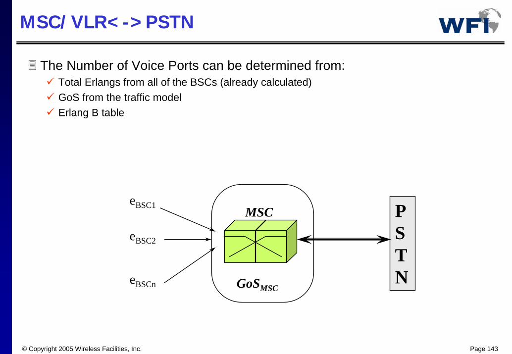
The Number of Voice Ports can be determined from:Total Erlangs from all of the BSCs (already calculated)GoS from the traffic modelErlang B table
MSC PSTN
eBSC1
eBSC2
eBSCn GoSMSC

© Copyright 2005 Wireless Facilities, Inc. Page 144
MSC/VLR Signaling links
The signaling links are based on a designed SS7 backbone: It is assumed that an existing network is used. And that the SS7 network is designed to handle the traffic from the PLMN.
All non-call-associated signaling in GSM is grouped under MAP (Mobile application part).
Non-call-associated signaling implies all signaling dealing with mobility management, security, activation/deactivation of supplementary services and so on.
Planning a fix SS7 packet network is a major task. Many large operators design their own SS7 network (STPs).
© Copyright 2005 Wireless Facilities, Inc. Page 145
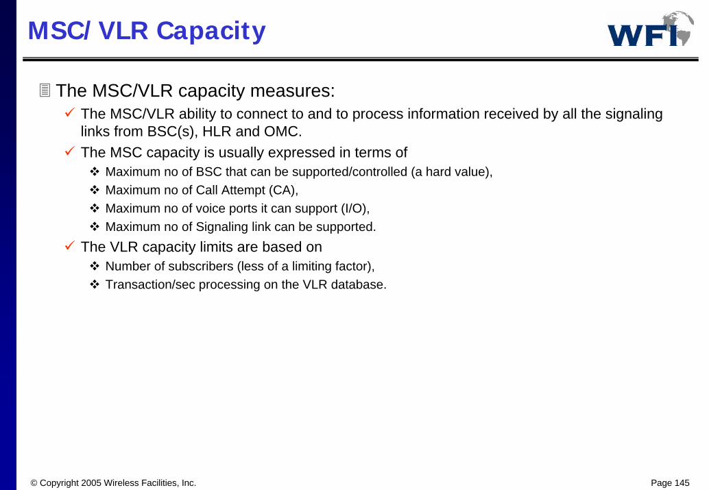
MSC/VLR Capacity
The MSC/VLR capacity measures:The MSC/VLR ability to connect to and to process information received by all the signaling links from BSC(s), HLR and OMC. The MSC capacity is usually expressed in terms of
Maximum no of BSC that can be supported/controlled (a hard value),Maximum no of Call Attempt (CA),Maximum no of voice ports it can support (I/O),Maximum no of Signaling link can be supported.
The VLR capacity limits are based onNumber of subscribers (less of a limiting factor),Transaction/sec processing on the VLR database.
© Copyright 2005 Wireless Facilities, Inc. Page 146
MSC/VLR Dimensioning
For a given system, once all of the voice ports and signaling links to the MSC have been identified, the size of MSC can be determined.
The total Erlang from all of the BSCs < Maximum Erlang supported by the MSC.The total number of voice ports required < Maximum ports supported by the MSC.The total CA from all of the BSCs < Maximum CA supported by the MSC.The total number of signaling links required < Maximum signaling links supported by the MSC.
© Copyright 2005 Wireless Facilities, Inc. Page 147
MSC/VLR Dimensioning (cont’d)
The VLR limitations must also be metTotal no. of subscribers < Maximum no. of subscribersTotal no. of transactions/sec < Maximum no. of transaction/sec
If the required traffic is greater than the MSC/VLR limits, then provide different alternatives
Increase the number of MSCs or plan for a larger MSC/VLRIf other MSCs already exist, then determine the possibility of sharing with other MSCs.
The best alternatives are selected based on system constraints.
© Copyright 2005 Wireless Facilities, Inc. Page 148
Distributed v.s. Centralized MSC Designs
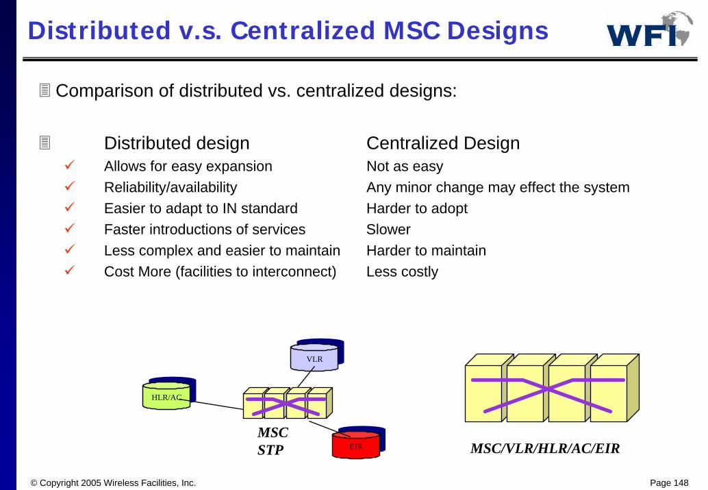
Comparison of distributed vs. centralized designs:
Distributed design Centralized DesignAllows for easy expansion Not as easyReliability/availability Any minor change may effect the systemEasier to adapt to IN standard Harder to adoptFaster introductions of services SlowerLess complex and easier to maintain Harder to maintainCost More (facilities to interconnect) Less costly
MSCSTP
HLR/ACHLR/AC
VLRVLR
EIREIR MSC/VLR/HLR/AC/EIR

© Copyright 2005 Wireless Facilities, Inc. Page 149
Planning/Configuration Steps
Review Inputs: Average Size and Capacity of Links and Network ElementsBTS Locations
BSC PlanningPreferred LocationsBTS-BSC ConfigurationsBTS-BSC Assignment
GMSC/MSC PlanningMSC Preferred LocationsBSC-MSC assignment
HLR Location, Redundant HLROMC Location
From Dimensioning
From RF Design
© Copyright 2005 Wireless Facilities, Inc. Page 150
Frequency Hopping
© Copyright 2005 Wireless Facilities, Inc. Page 151
Frequency Hopping
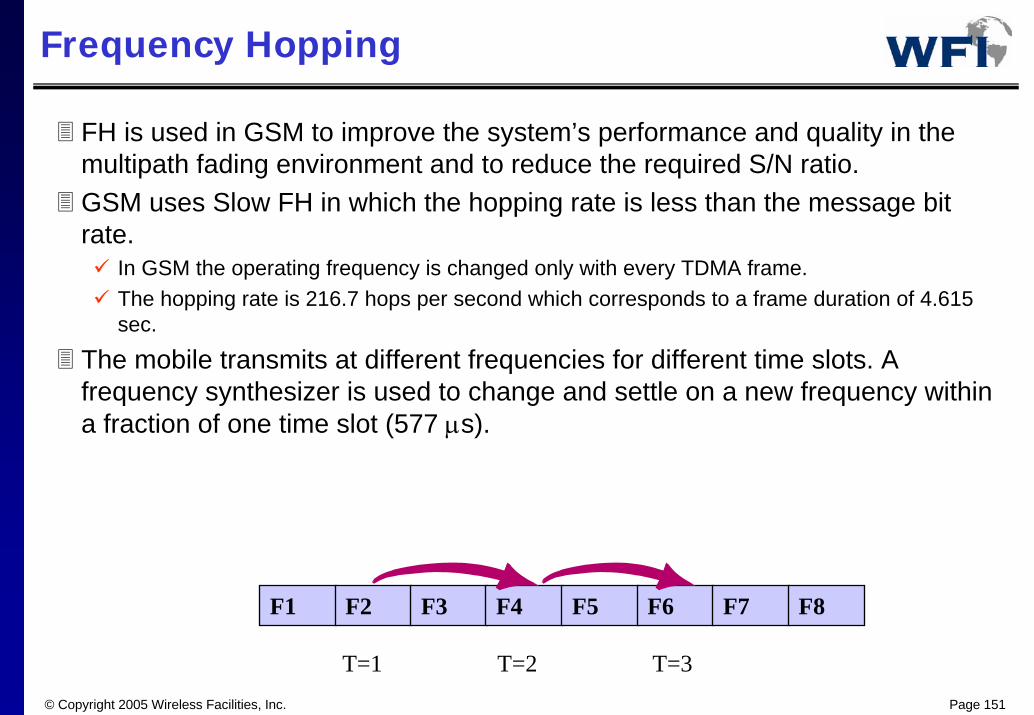
FH is used in GSM to improve the system’s performance and quality in the multipath fading environment and to reduce the required S/N ratio.GSM uses Slow FH in which the hopping rate is less than the message bit rate.
In GSM the operating frequency is changed only with every TDMA frame.The hopping rate is 216.7 hops per second which corresponds to a frame duration of 4.615 sec.
The mobile transmits at different frequencies for different time slots. A frequency synthesizer is used to change and settle on a new frequency within a fraction of one time slot (577 µs).
F1 F2 F3 F4 F5 F6 F7 F8
T=1 T=2 T=3
© Copyright 2005 Wireless Facilities, Inc. Page 152
Frequency Hopping (cont’d)
FH provides frequency diversity to overcome Rayleigh fading which may cause fades of 40 to 50 dB deep on the received signal.
FH also provides interference diversity (interference averaged over multiple users).
FH reduces the S/N ratio required for an acceptable QoS, from 12 dB for a non-hopping radio link to 9 dB (approx.), improving the overall network’s capacity.
Different hopping algorithms can be assigned to the MSCyclic Hopping Random Hopping
© Copyright 2005 Wireless Facilities, Inc. Page 153
Frequency Hopping (cont’d)
In the Mobile Station, in FH mode, only three time slots are available to transmit, receive and monitor while in the BTS all eight time slots are capable of transmitting and receiving to support eight MSs in one frame.
The Broadcast Channels (BCH) comprising of FCCH, SCH and BCCH are not allowed to hop.
All dedicated channel types can hop (TCH/SDCCH/FACCH/SACCH).
Two different implementation schemes of SFH are used in BSs which are base-band hopping and RF hopping.
Hybrid hopping is a combination and compromise of the two implementation schemes.

© Copyright 2005 Wireless Facilities, Inc. Page 154
Base-band Hopping
ANT
TS handler transmitter f0
TS handler transmitter f1
TS handler transmitter f2
TS handler transmitter f3
TRX 1
TRX 2
TRX 3
TRX 4
filtercombiner
Bus for routing of bursts
Each transmitter is assigned with a fixed frequency. At transmission, all bursts, irrespective of which connection, are routed to the appropriate transmitter of the proper frequency. The mobile is hopped around the transmitters and receivers.The advantage with this mode is that narrow-band low loss filter combiners can be used.
© Copyright 2005 Wireless Facilities, Inc. Page 155
Base-band Hopping (cont’d)
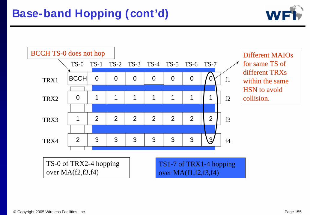
BCCH TSBCCH TS--0 does not hop0 does not hop
BCCH 0 00 000
TS-0 TS-1 TS-2 TS-3 TS-4 TS-5 TS-6
0
TS-7
TRX1
1 1 1 1 11 1
2 2 2 22 2
3333333
2
TRX2
TRX3
TRX4
f1
f2
f3
f4
0
1
2
TS-0 of TRX2-4 hoppingover MA(f2,f3,f4)
TS1-7 of TRX1-4 hoppingover MA(f1,f2,f3,f4)
Different MAIOsDifferent MAIOsfor same TS of for same TS of different TRXsdifferent TRXswithin the same within the same HSN to avoid HSN to avoid collisioncollision.
© Copyright 2005 Wireless Facilities, Inc. Page 156
RF Hopping
TS handler transmitter f0 . . . fn
TS handler
TS handler
TS handler
TRX 1
TRX 2
TRX 3
TRX 4
transmitter f0 . . . fn
transmitter f0 . . . fn
transmitter f0 . . . fn
ANThybridcombiner
ANThybridcombiner
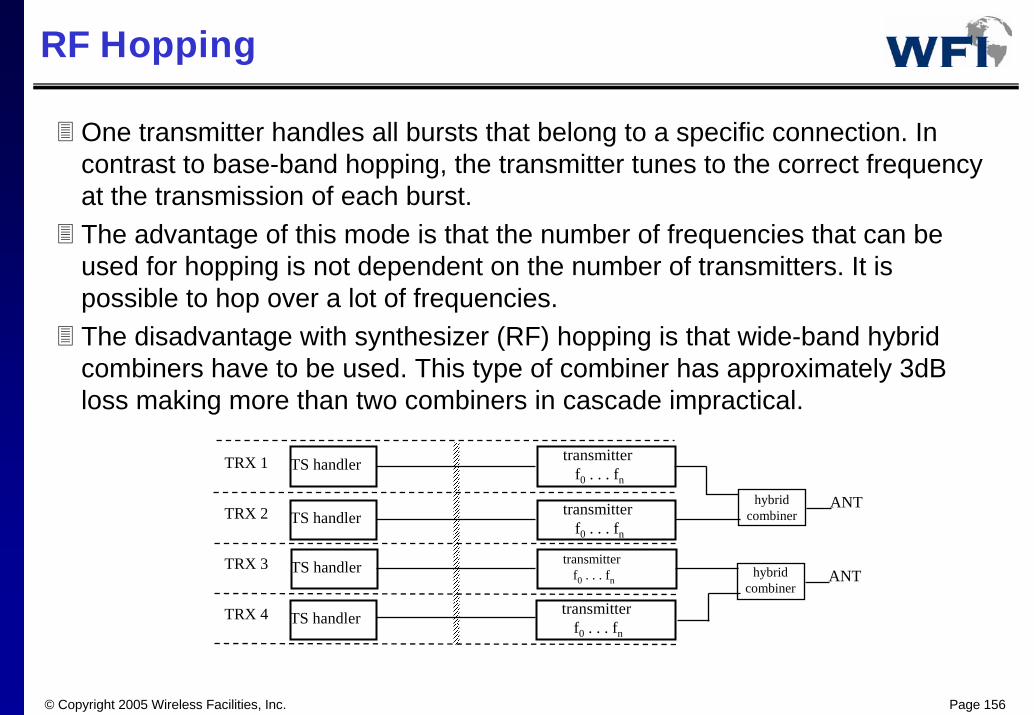
One transmitter handles all bursts that belong to a specific connection. In contrast to base-band hopping, the transmitter tunes to the correct frequency at the transmission of each burst.The advantage of this mode is that the number of frequencies that can be used for hopping is not dependent on the number of transmitters. It is possible to hop over a lot of frequencies.The disadvantage with synthesizer (RF) hopping is that wide-band hybrid combiners have to be used. This type of combiner has approximately 3dB loss making more than two combiners in cascade impractical.
© Copyright 2005 Wireless Facilities, Inc. Page 157
RF Hopping (cont’d)
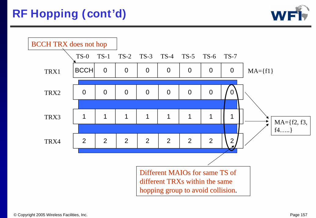
BCCH TRX does not hopBCCH TRX does not hop
BCCH 0 00 000
TS-0 TS-1 TS-2 TS-3 TS-4 TS-5 TS-6
0
TS-7
TRX1
0 0 0 0 0
1 1 1 11 1
2222222
1
TRX2
TRX3
TRX4
MA={f1}
0
1
2
Different MAIOs for same TS of Different MAIOs for same TS of different TRXs within the same different TRXs within the same hopping group to avoid collisionhopping group to avoid collision..
0 0
MA={f2, f3, f4…..}

© Copyright 2005 Wireless Facilities, Inc. Page 158
Hopping Algorithms
Cyclic frequency hopping: the frequencies are changed, once every TDMA frame, in a consecutive order (e.g. …,f1,f2,f3,f4,f1,f2,f3,f4,…).
Random frequency hopping: a random hopping sequence is implemented as a pseudo-random sequence. 63 independent sequences are defined.
Hopping Sequence Number (HSN) will specify which of the 63 sequences to be used (e.g. …,f1,f4,f4,f3,f1,f2,f4,f1,…).
The random hopping mode is superior for averaging the co-channel interference. Random hopping is the hopping mode of choice for high capacity networks.
© Copyright 2005 Wireless Facilities, Inc. Page 159
Hopping Algorithms (cont’d)
Orthogonal hopping sequence: for each transceiver, in the same channel group, in the same cell, they will be assigned with the same HSN, i.e. they hop in the same way.
In order not to interfere with each other, they must not use the same frequency at the same time. The problem is solved by using an offset in the hopping sequence, referred to as Mobile Allocation Index Offset (MAIO). Two transceivers bearing the same HSN but different MAIO will never use the same frequency in the same TDMA frame.
(e.g., …,f1,f4,f4,f3,f1,f2,f4,f1,……,f2,f1,f1,f4,f2,f3,f1,f2,……,f3,f2,f2,f1,f3,f4,f2,f3,……,f4,f3,f3,f2,f4,f1,f3,f4,…).