revuz, julia (2011) numerical simulation of the wind flow around a
TRANSCRIPT

Revuz, Julia (2011) Numerical simulation of the wind flow around a tall building and its dynamic response to wind excitation. PhD thesis, University of Nottingham.
Access from the University of Nottingham repository: http://eprints.nottingham.ac.uk/13151/1/555518.pdf
Copyright and reuse:
The Nottingham ePrints service makes this work by researchers of the University of Nottingham available open access under the following conditions.
This article is made available under the University of Nottingham End User licence and may be reused according to the conditions of the licence. For more details see: http://eprints.nottingham.ac.uk/end_user_agreement.pdf
For more information, please contact [email protected]

Numerical simulation of the wind flow
around a tall building and its dynamic
response to wind excitation
Julia Revuz
Supervisors: Dr. David Hargreaves and Dr. John Owen
Department of Civil Engineering, Faculty of Engineering,
University of Nottingham
Thesis submitted to the University of Nottingham
for the degree of Doctor of Philosophy
April 2011
GEORGE GREEN LIBRARY W SCIENCE AND ENGINEERING

Abstract
Wind action is particularly important for tall buildings, both in providing a signifi-
cant contribution to the dynamic overall loading on the structure and by affecting its
serviceability. Whereas low and medium-rise buildings are fairly rigid, tall structures
are characterized by a greater flexibility and a lower natural frequency, which is more
likely to be in the frequency range of wind gusts. In addition, wake effects, such as vor-
tex shedding, can become a significant problem for flexible structures when the vortex
shedding frequency is close to the natural frequency of the building.
The aim of the present thesis is to assess the validity of commercial CFD codes for
modelling the wind flow around a high-rise building, including the consideration of the
coupled dynamic response of the building to turbulent wind loading. Three intermediate
objectives are set.
The first is to develop a tool to couple fluid and structure in a sequential manner. The
equations for the air flow are solved using the commercial CFD program ANSYS-Fluent.
The response of the structure is found from solving the structural response with a modal
approach, the response in each vibration mode being treated as a SDOF problem. This
fluid-structure interaction tool is applied to model a 180 m building, allowed to move in
the across wind direction. The second objective is to investigate and find a method to
generate fully turbulent inflow for LES in order to reproduce an accurate wind spectrum.
The chosen method is tested and validated in an empty fetch. Ultimately, both tools
are brought together and applied to model a 180 m building, which is allowed to bend
in the along wind and across wind directions. Finally, the third intermediate objective

brings together the tools developed in the first and second intermediate objective to
model the dynamic response of a 180 m building to dynamic wind loading, within a
turbulent inflow, using LES.
11

Acknowledgements
This thesis would not have been possible without the support, in various ways, of a
number of people. First of all, I am deeply grateful to my main supervisor, Dr David
Hargreaves, for his endless patience and knowledge sharing. I would also like to thank
Dr John Owen for his support and his ability to make me see the bigger picture and not
get lost in the details. I would also like to thank Dr Herve Morvan for always taking
interest in my work and adding an external perspective to the project.
I would also like to thank Dr Zhengtong Xie for his collaboration on the turbulent inflow
generation method used for this research.
In my daily work, I have to thank Bruce Kakimpa for all the fruitful discussions about
everything related to CFD, but not only: politics was definitely a favourite topic of
conversation whenever we had had enough of CFD, or Gambit had exhausted all of our
energy!
I am deeply grateful to my family for the support and encouragement I received through-
out my studies.
As for the writing-up, I would like to thank Rachel Thomas, for taking the time to proof
read most of my thesis, and helping me make the text much clearer.
Finally, what made these three years such a great experience on every possible level is
definitely working in a multicultural environment alongside some amazing people in the
department. So, a huge thanks to my friends Jeff, Meinard, Paloma, Diego, Fangfang,
Riccardo, Andy, Kawran...
111

Contents
1 Introduction 11
1.1 Context ..... ...... ......... .... .... ..... ...
11
1.2 Aims and Objectives ............................. 13
2 Introduction to Wind Engineering 17
2.1 The Atmospheric Boundary Layer ..................... 17
2.1.1 Introduction .............................
17
2.1.2 Basic assumptions .......................... 20
2.1.3 Governing equations ......................... 20
2.1.4 Mean velocity and roughness height ................ 22
2.1.5 Atmospheric turbulence .................... ... 26
2.1.6 Turbulence intensity, Reynolds stresses and length scales ..... 29
2.1.7 Wind spectra ............................. 34
2.2 Response of tall buildings to wind loading ................. 37
2.2.1 Introduction: building aerodynamics ................ 37
2.2.2 Aeroelastic phenomena ....................... 41
2.2.3 Structural dynamics ......................... 45
2.3 Summary and conclusions .......................... 50
iv

CONTENTS
3 Literature Review of Computational Wind Engineering 52
3.1 Introduction on Computational Wind Engineering ...... ... ...
52
3.1.1 CFD in wind engineering ...................... 52
3.1.2 CFD methodology .......................... 54
3.1.3 Discretization of the governing equations ............. 55
3.1.4 The computational grid ....................... 61
3.2 Introduction to turbulence modelling .................... 64
3.3 RANS approach for turbulence modelling in wind engineering ...... 65
3.3.1 The k-e turbulence model ...................... 65
3.3.2 The Menter SST k-w turbulence model .... ... .... ... 70
3.3.3 The Reynolds Stress Models (RSM) .... .... . .... ... 73
3.3.4 Boundary conditions for RANS-based models ........... 74
3.3.5 URANS ................................ 77
3.4 Large Eddy Simulation (LES) ........................ 77
3.4.1 Governing equations ......................... 77
3.4.2 The key SGS models ...... .... . .... ... . ... ... 79
3.5 Hybrid RANS/LES models ........ . .... .... ..... ... 86
3.6 Summary and conclusions ....................... ... 91
4 Size of the computational domain 92
4.1 Introduction .................................. 92
4.2 Background .................................. 92
4.3 Case study ............................... ... 95
4.3.1 Domains and meshes ......................... 95
4.3.2 Turbulence model, boundary and initial Conditions ... ..... 98
V

CONTENTS
4.3.3 Solver settings ............................ 99
4.4 Results and discussion ............................ 100
4.5 Summary and new recommendations .................... 107
4.6 Application of the new recommendations .................. 108
4.7 Conclusions .................................. 113
5 Fluid-structure interactions 114
5.1 Introduction .................................. 114
5.2 Review of the method for modelling fluid-structure interactions ..... 114
5.2.1 Introduction ............................. 114
5.2.2 Fluid-mesh coupling ......................... 115
5.2.3 Fluid-structure coupling schemes .................. 117
5.2.4 Discretization ............................. 121
5.2.5 Applications to CWE ........................ 121
5.3 The method for modelling fluid-structure interaction ........... 125
5.3.1 Introduction ............................. 125
5.3.2 The structural solver: modal superposition approach . ... ... 125
5.3.3 Application of the method ... .... ....... ..... ... 130
5.3.4 Summary of the FSI coupling method ............... 134
5.4 Application of the FSI method to a1 in 200 scale building ........ 137
5.4.1 Introduction ............................. 137
5.4.2 Set-up ................................. 138
5.4.3 Methodology ............................. 140
5.4.4 Results and discussion ........................ 140
5.5 Summary and conclusions ... .... .... ............... 142
vi

CONTENTS
6 Turbulent Inflow 145
6.1 Introduction .................................. 145
6.2 Description of the method for generating turbulent inflow for LES ... 147
6.3 Application of the method: the UDF . ....... .... ..... ... 157
6.3.1 Structure of the UDF ........................ 157
6.3.2 Generation of the random data ......... .......... 159
6.3.3 The Reynolds stress tensor distribution .............. 160
6.4 Verification: the empty fetch test case ................... 160
6.4.1 Introduction ............................. 160
6.4.2 Empty fetch test case: set-up .................... 161
6.5 Verification: the empty fetch test case, the results ............. 164
6.5.1 Characteristics of the generated synthetic turbulent inlet .... 164
6.5.2 Behaviour of the turbulent inflow along the domain .... ... 174
6.6 Summary and conclusions .......................... 180
7 Combination of turbulent inflow for LES and FSI method 182
7.1 Introduction .... ... .... ...... .... ..... ..... . .. 182
7.2 Method .... .... ...... ... ...... ... .... .... .. 184
7.3 Set-up ..................................... 184
7.4 Results and Discussion ............................ 186
7.5 Conclusions ..................................
193
8 Conclusions and Recommendations 196
8.1 Summary ...................................
196
8.2 Critical appraisal . ....... .... .... ............... 198
vii

CONTENTS
8.3 Conclusions .................................. 199
8.4 Further work . ...... .... ......... .... .... ... .. 199
References 201
Appendices 214
Appendix A The ALE formulation for mesh-fluid coupling 215
Appendix B Program for Fluid Structure Interactions 219
B. 1 Finite Element Method: openFEM .... .... ....... .... .. 219
B. 2 Running the flow solver ANSYS-Fluent with fluid-structure interactions 219
B. 3 The FSI program (the UDF): functions and Macros ........... 220
B. 3.1 Auxiliary functions in the UDF .... ....... ...... .. 220
B. 3.2 Main body of the UDF .......... ..... ....... . 221
B. 4 The UDF for FSI . ............. .... ..... ...... ..
222
B. 4.1 Parallelisation of the code ...................... 222
B. 4.2 The UDF ........... .................... 223
Appendix C UDF for time-varying turbulent inflow 241
C. 1 Auxiliary functions in the UDF ....................... 241
C. 2 Scheme .................................... 241
C. 2.1 Main body of the UDF .... ...... ..... .... ... . 242
C. 3 The UDF ... ...... .... ... .... ..... .... . .... . 243
Appendix D Statistics 264
D. 1 Temporal autocorrelation .................... ...... 264
D. 2 Spatial autocorrelation ...... ..... ...... ... ........ 265
1

List of Figures
2.1 Composition of the ABL ...........................
18
2.2 Lapse rates for the three states of the ABL .................
20
2.3 Roughness effects on the velocity profile ....... .... ..... ... 25
2.4 Effect of roughness change on velocity profile ................ 25
2.5 Illustration of vortex stretching ........................ 27
2.6 Reynolds stresses distribution in a boundary layer ....... . ..... 30
2.7 Reynolds stresses distribution in the ABL .................. 31
2.8 Length scales (after ESDU 85020 (1985, revised in 1990)). ........ 33
2.9 van der Hoven Spectrum ...........................
34
2.10 Wind spectra over rough terrain . ..... ..... ...... ...... 36
2.11 Coherence functions (after Simiu and Scanlan (1986)). .......... 37
2.12 Air flow pattern around a building, side view ........ ..... ... 38
2.13 Horseshoe vortex after Cook (1992) ..................... 39
2.14 Flow past a rectangular cylinder ....................... 40
2.15 Vortex-formation model showing entrainment flows. ...........
40
2.16 Incident flow not normal to the building: the Delta wing vortices.. ... 42
2.17 Wind response directions (after Mendis et al. (2007)). ..........
42
2.18 Free vibration of a cylinder: lock-in phenomenon .... .......... 44
2

LIST OF FIGURES
2.19 Aerodynamic admittance function (after Houghton and Carruthers (1976)). 49
2.20 Forces spectra (after Davenport (1995)) ...................
50
3.1 Structured and unstructured mesh ......... ............. 57
3.2 Discretization and Solver for the flow equations .............. 61
3.3 Numerical Diffusion ..............................
62
3.4 Mesh quality: Aspect ratio and Skewness . .... ..... ....... . 63
3.5 Law of the wall (after Blocken et al. (2007)) . .... ... ...... ..
67
3.6 Adjacent cell to the wall, zp in the Figure refers to yp in Equation 3.3.7. 68
3.7 Turbulent kinetic energy distribution around a cube. ..... .... .. 69
3.8 Effects of a shear stress applied at the top boundary on velocity profile. 76
3.9 Comparison of the standard k-e model and LES .............. 84
3.10 Pressure coefficients on cube after Lim et al. (2009). ........... 86
3.11 Flow regions in DES (modified version of a sketch by Spalart (2001)). . 88
3.12 RANS and LES regions (after Davidson and Peng (2003)).. ....... 89
3.13 Hybrid RANS-LES and zonal approach after Tessicini et al. (2006).. ..
90
4.1 Computational domain taken from Franke (2007) . .... ....... . 93
4.2 Dimensions of the four domains. .". """""""............ 97
4.3 Surface meshes for the small domain .""""".............. 98
4.4 Contours of velocity magnitude at midheight ............... 101
4.5 Contours of velocity magnitude on vertical plane ............. 102
4.6 Comparison of velocity profiles across fetch ................ 103
4.7 Comparison of wake width and wake depression .............. 104
4.8 Pressure coefficients distribution on the building . ...... . ..... 105
3

LIST OF FIGURES
4.9 Contours of velocity magnitude at midheight with FR ..........
109
4.10 Contours of velocity magnitude on vertical plane with FR ...... ..
110
4.11 Comparison of velocity profiles across fetch with FR ... ...... .. 110
4.12 Comparison of wake width and wake depression including FR ...... 111
4.13 Pressure coefficients distribution on the building with FR ........
112
5.1 ALE mesh-fluid coupling ........................... 116
5.2 Conventional and staggered sequential coupling schemes.. ........ 118
5.3 Times histories of the lift and drag from Braun and Awruch (2009). .. 123
5.4 Time histories of the response from Braun and Awruch (2009). ..... 124
5.5 Amplitude response to harmonic loading . .... ..... ...... .. 129
5.6 Phase response to harmonic loading .""""""............. 130
5.7 Elements types in Ansys-Fluent ....................... 131
5.8 Procedure for dynamic meshing ....................... 132
5.9 Adjacent cells to moving mesh ....................... 134
5.10 Sequential Procedure for fluid-structure coupling . .... .... .... 136
5.11 Geometry and mesh of the 180 m building and its rigid rigid zone ... 139
5.12 Times history of the lift force acting on the building ........... 141
5.13 Times history of the response of the building ............... 142
5.14 Flow field: velocity magnitude at midheight of the building ....... 143
5.15 Vortex shedding frequency vs reduced velocity ... ...... ..... . 144
6.1 Filter coefficients by ............................. 148
6.2 Filtering of the random data: illustration ................. 154
6.3 2D set of random data, raw and filtered . ..... .... ....... . 154
4

LIST OF FIGURES
6.4 Bilinear interpolation from virtual uniform mesh to CFD mesh ..... 155
6.5 Summary of the method for generating turbulent inflow ......... 156
6.6 Flow chart of the UDF for turbulent inflow in the Fluent solver ..... 158
6.7 Domain for the empty fetch test case .................... 162
6.8 Empty fetch test case: time history of the velocity magnitude ...... 165
6.9 Empty fetch test case: contours of the velocity .............. 166
6.10 Empty fetch test case: autocorrelation plots of the X-velocity ...... 170
6.9 Empty fetch test case: spatial autocorrelation of the X-velocity ..... 172
6.9 Empty fetch test case: power spectrum of the longitudinal velocity ... 173
6.10 Empty fetch test case: cross-spectrum of the longitudinal velocity .... 174
6.11 Empty fetch test case: temporal autocorrelation across fetch ....... 176
6.12 Empty fetch test case: longitudinal length scales at different heights .. 176
6.13 Empty fetch test case: Longitudinal spectrum across the domain .... 177
6.14 Empty fetch test case: Cross covariance of longitudinal velocity ... .. 179
7.1 Framework, combination of turbulent inflow and FSI. . .... ..... 184
7.2 Domain with rigid zone ............................ 185
7.3 Velocity profile at x= 20L upstream the building ............. 187
7.4 Profiles of rms velocity upstream the building ............... 188
7.5 Iso surfaces of vorticity ............................ 189
7.6 Iso surfaces of II ................................
190
7.7 Contours of vorticity on a horizontal plane ................. 190
7.8 Pressure distribution on the building .................... 192
7.9 Contours of static pressure distribution ................... 193
7.10 Response of the building . .... . .... . ........... ..... 194
5

LIST OF FIGURES
7.11 Trajectory covered by the roof center point ................. 194
A. 1 The three frames of references in ALE ... ... .... .... .... ..
216
B. 1 Diagram of the architecture of parallel computing in Ansys-Fluent ... 223
C. 1 Screenshot of the menus for the turbulent inflow .............. 242
6

List of Tables
2.1 Typical Roughness Lengths .......................... 24
3.1 Standard and Revised k-e turbulence models ................ 69
4.1 Domain sizes from relevant CFD modelling of tall buildings.. .... .. 94
4.2 Characteristics of the domains ........................ 96
4.3 Characteristics of the mesh following the Final Recommendations (FR). 108
6.1 Summary of the set up for the empty fetch test case ........... 163
6.2 Empty fetch test case: Time scales ..................... 169
6.3 Empty fetch test case: Spatial length scales ................ 169
6.4 Empty fetch test case: Spatial Length scales . ... . ... .... . ... 170
7

PAGINATED BLANK PAGES
ARE SCANNED AS FOUND IN ORIGINAL
THESIS
NO INFORMATION
MISSING


LIST OF TABLES
Notations
A. Frequency of vortex shedding s-1
A Natural frequency of the building s-1
9X Along wind displacement of the structure m
gy Across wind displacement of the structure m
h Height of the building m
k Turbulent kinetic energy m2 s-2
Li Length scales of turbulence (i = u, v, v and j=x, y, z) m
Re Reynolds number
St Strouhal number
u Longitudinal component of the wind speed rn s-1
U Mean longitudinal component of the wind speed m s-1
U1 Fluctuating longitudinal component of the wind speed m s-1
ux, uy, u, z Components of the velocity of the wind in Chapter 6 m s-1
U, Friction velocity m 8-1
Uref Reference wind speed m 8-1
V Horizontal component of the wind speed m s-1
V/ Fluctuating horizontal component of the wind speed m s-1
w Vertical component of the wind speed m s-1
w/ Fluctuating vertical component of the wind speed m 8-1
y Structure displacement m
zo Roughness length m
z9 Gradient height In
ziel Reference height m 9

LIST OF TABLES
e Turbulent dissipation rate (fluid) m2 s-3
K Von Karman constant
µ Air dynamic viscosity m2 s-2
V Air kinematic viscosity m2 s-1
Structural damping ratio
p Air density kg m-3
au, a, o-,,, Components of the standard deviation of the wind speed m s-1
Shear stresses in the ABL kg m-1 s-2
Mode shapes in the along-wind direction of the structure
ýGn Mode shapes in the across-wind direction of the structure
w Specific dissipation rate (k-w turbulence model) s-1
10

Chapter 1
Introduction
1.1 Context
Computational Wind Engineering
The Wind Engineering Society defines Wind Engineering as a multidisciplinary sub-
ject concerned with the effects of wind on the natural and built environment. This
includes investigation of pollutant dispersion and pedestrian comfort assessment, but
also most important for the present work: the study of the wind loads on buildings and
the aerodynamic phenomena caused by the interaction of the air-flow and the surface
structures.
Computational Wind Engineering (CWE) is the application of Computational Fluid
Dynamic (CFD) techniques to wind engineering and aims to predict the wind loads
on buildings and the air flow around them. CWE only became feasible twenty years
ago with the rapid increase of computer speed and memory capacities. Even so, for
many years, computer resources have not allowed complex calculations, being restricted
to steady-state BANS (Reynolds Averaged Navier Stokes) turbulence modelling. In
the last five years, transient simulations using Large Eddy Simulation (LES), applied
to large grids, have demonstrated that CWE can reach a good level of accuracy and
potentially compete with wind-tunnel studies.
11
CHAPTER 1: INTRODUCTION
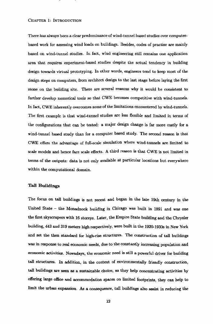
There has always been a clear predominance of wind-tunnel based studies over computer-
based work for assessing wind loads on buildings. Besides, codes of practise are mainly
based on wind-tunnel studies. In fact, wind engineering still remains one application
area that requires experiment-based studies despite the actual tendency in building
design towards virtual prototyping. In other words, engineers tend to keep most of the
design steps on computers, from architect design to the last stage before laying the first
stone on the building site. There are several reasons why it would be consistent to
further develop numerical tools so that CWE becomes competitive with wind-tunnels.
In fact, CWE inherently overcomes some of the limitations encountered by wind-tunnels.
The first example is that wind-tunnel studies are less flexible and limited in terms of
the configurations that can be tested: a major design change is far more costly for a
wind-tunnel based study than for a computer based study. The second reason is that
CWE offers the advantage of full-scale simulation where wind-tunnels are limited to
scale models and hence face scale effects. A third reason is that CWE is not limited in
terms of the outputs: data is not only available at particular locations but everywhere
within the computational domain.
Tall Buildings
The focus on tall buildings is not recent and began in the late 19th century in the
United State - the Monadnock building in Chicago was built in 1891 and was one
the first skyscrapers with 16 storeys. Later, the Empire State building and the Chrysler
building, 443 and 319 meters high respectively, were built in the 1920-1930s in New York
and set the then standard for high-rise structures. The construction of tall buildings
was in response to real economic needs, due to the constantly increasing population and
economic activities. Nowadays, the economic need is still a powerful driver for building
tall structures. In addition, in the context of environmentally friendly construction,
tall buildings are seen as a sustainable choice, as they help concentrating activities by
offering large office and accommodation spaces on limited footprints, they can help to
limit the urban expansion. As a consequence, tall buildings also assist in reducing the
12
CHAPTER 1: INTRODUCTION
carbon footprint by reducing transport across a sprawling metropolis.
The design of tall buildings faces two main challenges that CWE can help to answer.
On the one hand, the combination of tall buildings and dense urban environment sig-
nificantly reinforces aeroelastic phenomena, such as wake effects and buffeting (to be
defined in section 2), which then considerably modifies and complicates the wind load-
ing problem. In fact, the wake effects play an important role for the buildings located
downstream of the structure that caused them. As a result, the flow field around tall
buildings presents particular features that need to be carefully studied, especially near
the ground where strong downward flows can perturb the environment for pedestrians
and also in the wake, downstream of the structure. On the other hand, whereas low and
medium-rise buildings are fairly rigid, tall structures are inevitably more flexible. This
makes them more sensitive to wind loading excitation and implies a significant dynamic
response. Therefore, tall buildings involve the association of complex flow fields mod-
ified by aerodynamic phenomena, and hence a substantial dynamic response that may
have an influence back on the fluid flow.
If many researches have worked on the numerical simulation of the dynamic response
of tall buildings, and others have been interested in the key features of the flow field
around tall buildings, both interests have not often been combined. Consequently, it
is of main importance to develop numerical tools for studying the flow field around
high-rise buildings accounting for their dynamic response. It is believed that existing
commercial CFD codes offer a sufficiently advanced and flexible basis to address the
challenges involved in modelling the flow field around tall buildings including the effects
of their dynamic response.
1.2 Aims and Objectives
The aim of the present work is to assess the ability of commercial CFD codes for mod-
elling the wind flow around a high-rise building - including the consideration of the
coupled dynamic response of the building to turbulent wind loading - by bringing to-
13

CHAPTER 1: INTRODUCTION
gether existing tools. This should establish a framework for modelling building response
to wind loading within a turbulent atmospheric boundary layer.
The main objectives of the present work are:
1. To develop and evaluate a numerical tool in order to account for the dynamic
response of the building to wind loading, and to assess the coupling of the building
motion and the wind flow.
2. To develop a suitable method for generating turbulent inflow for unsteady LES
simulations and to assess the use of LES combined with the method for turbulent
inflow in the modelling of wind flow around tall buildings.
3. To combine and evaluate the performances of the combination of 2) the coupling of
the dynamic response of the tall building with the modelling of the wind flow, and
3) the technique for producing turbulent inflow, in an unsteady LES simulation.
14

CHAPTER 1: INTRODUCTION
Summary of chapters
Chapter 1 introduces the thesis with a very general background of the history of the
tall buildings and wind engineering, and sets the main goal of this work with associated
intermediate objectives.
Chapter 2 introduces the field of wind engineering and presents the important fea-
tures of the flow around buildings and the main characteristics of the Atmospheric
Boundary Layer, as well as the general method to study the building response.
Chapter 3 presents a literature review of the application of CFD to wind engineering
problems, mainly focusing on turbulence modelling.
Chapter 4 presents the results of an investigation of the optimal dimensions of the
computational domain to use to numerically study the flow around tall buildings. The
main conclusion is that the computational domain can be greatly reduced from the
general guidelines, which were derived for low to mid-rise buildings. The chapter suggests
new guidelines for the size of the computational domains to be applied to tall buildings.
Chapter 5 develops the method that has been determined to couple fluid and struc-
ture using an existing CFD code. This method is then applied to a cantilever, which
is allowed to move in the transversal direction. "Lock-in" phenomenon was found to
happen for reduced velocity of about 1.1.
Chapter 6 presents the investigation and the optimisation of a method to generate
turbulent inflow for LES. The generator is applied to an empty fetch test case in order
to verify and validate the approach.
Chapter 7 presents the results of a study combining the main two tools developed in
Chapters 5 and 6 in order to meet the main objective of this work.
15

CHAPTER 1: INTRODUCTION
Chapter 8 finally summarizes the main findings of this thesis and suggests some
further recommendations.
16

Chapter 2
Introduction to Wind
Engineering
2.1 The Atmospheric Boundary Layer
2.1.1 Introduction
From a wind engineering point of view, the region of the Earth's atmosphere of interest
is the Atmospheric Boundary Layer (ABL), which can cover the lowest kilometre or so
of the atmosphere.
Garrat (1992) defines the ABL as the part of "the Earth's surface where the effects of
the surface, such as friction, heating, and cooling, are felt directly on a time scale of less
than a day, and in which significant fluxes of momentum, heat or matter are carried by
turbulent motions on a scale of the order of the depth of the boundary layer or less".
Two main layers can be distinguished in the ABL (Figure 2.1):
" the inner region called the Surface Layer, mainly influenced by the surface features.
The Surface layer is composed of the Interfacial layer, and the Inertial sub-layer.
The Inertial sub-layer allows the transition between the inner region and the outer
region.
17

CHAPTER 2: INTRODUCTION TO WIND ENGINEERING
I ............ Gradientlieigbt H, (! 1-5km)...
Edunan lay
a as a
Surface layer (-0.1H) ý Iw, w mow.
al nleyer ýacertent
f-I
i
-I T7 II
-I- --- ntafedv-pla
Figure 2.1: Composition of the ABL: The Surface layer composed of the Interfacial layer, and the Inertial sublayer; and the Eckman layer.
" the outer region, also called the Eckman Layer, where the dominant factor is the
Earth's rotation.
The turbulent shear stress or Reynolds stress, defined in section 2.1.4, varies with the
height through the ABL as follows: it is equal to zero at the ground level, reaches a
maximum at the top of the interfacial layer, and then decreases to vanish at the top of
the boundary layer, where the velocity reaches the gradient velocity, V..
The Interfacial layer covers approximately four fifths of the average building height.
There is no general direction for the wind flow within this layer but many local directions,
due to the buildings locations creating channels for the wind flow. Consequently, the
overall net flow is zero, which is why the depth of the interfacial layer is often called
the zero-plane displacement height and denoted zd. The zero plane displacement height
strongly depends on the surface roughness: in urban areas, where structures contribute
to a significant increase in surface roughness, this depth is important. In open country,
where the Interfacial layer is not significant, the Eckman layer is predominant.
Wind motion in the Eckman layer is determined by the pressure force due to the static
pressure field, and by the Coriolis force from the Earth's rotation. The former acts
normal to the isobars and the latter acts normal to the wind direction (Cook, 1992). In
other words, within that layer the pressure gradient effects and the Coriolis effects are
18

CHAPTER 2: INTRODUCTION TO WIND ENGINEERING
the two dominant phenomena.
The overall depth of the ABL depends on the atmospheric conditions but generally
varies between a few hundreds metres to several kilometres, depending on the location.
Depending on the influence of the thermal effects, the ABL will be considered unstable,
neutral, or stable.
Let us first define the lapse rate: it is the rate of temperature decrease with height of a
parcel of air in the ABL. Under adiabatic conditions (where no heat is exchanged) and
for an unsaturated mass of air, the lapse rate is the Dry Adiabatic Lapse Rate (DALR),
and the three states of the ABL can be characterized relatively to the DALR, as shown
in Figure 2.2 (a), neutral, stable or unstable.
In order to illustrate what happens in each case, consider a mass of warm air near
the surface; as this air is warmer, it rises, and the low pressure causes the mass of air
to expand in an adiabatic cooling process. If the mass of air does not cool down to
the level of the surrounding air, then it will continue to rise, creating large convection
cells, causing the boundary layer to be thick with large scale turbulent eddies. This
situation is considered unstable and is likely to occur on warm days, where the decrease
of temperature is not as steep as in DALR conditions as illustrated in Figure 2.2(a).
However, if the adiabatic cooling process brings the mass of air to thermal equilibrium
with the surrounding air, then the air will stop rising, and the boundary layer is then
considered stable, this typically occurs when the ground is colder, for example on cool
nights. Finally, if there are strong winds causing sufficient mixing to maintain thermal
equilibrium through the adiabatic cooling process, then the ABL is considered to be
neutral. This last case is the most important in wind engineering applications, as it is
the state of the ABL with strong winds and high turbulence levels. The displacement
of a mass of air in a neutral ABL is illustrated in Figure 2.2 (b). (Simiu and Scanlan,
1986; Burton et al., 2002)
19

CHAPTER 2: INTRODUCTION TO WIND ENGINEERING
400
350
300 DALR
250 E
200
150 Unal
100
50
0
Neutral
19 195 20 20.5 21 21.5 22
Temperatve ( dune celdW)
(a) (b) Figure 2.2: Lapse rates for a stable, neutral and unstable ABL (a) and illustration of the displacement of a mass of air in a neutral ABL (after Dyrbye and Hansen (1997)).
2.1.2 Basic assumptions
Two main assumptions need to be made to simplify the resolution of the ABL motion.
Firstly, in the present work, the ABL is considered neutrally stable, that is, heat con-
vection is neglected compared to mechanical turbulence. The mechanical turbulence
produces enough mixing to swamp movements due to the thermal effects. This assump-
tion can be made as structural engineers are mainly concerned with the effects of strong
winds, with high Reynolds numbers, hence high turbulence levels.
In addition, incompressibility is assumed for the wind flow.
2.1.3 Governing equations
The governing equations for the wind motion within the neutrally stable ABL are as
follows
0996
at
0946
+(ýax 49U
+vay au 1 ap
+w8z)+pox 1 a'
-fv+p8z (2.1.1)
av at
av +(u ax
av +v ay
av 1 ap _- +w19Z
pOy 1ar
-f U+ P äz
(2.1.2)
aw äw +(u
äw +v
aw 109P )+- +wä - 1 aT
+g=-- (2.1.3) at äx ay z p 09Z Pz
20

CHAPTER 2: INTRODUCTION TO WIND ENGINEERING
äu av ew p(x+-+Viz)=0 (2.1.4)
where u, v, w are the velocity components along the x, y, z axes respectively, where x is
the along-wind axis, y the cross-wind axis, and z the vertical axis. p is the air density,
p the pressure, g the acceleration of gravity, and Tu, r, and r,,, are the shear stresses.
The first terms on the right-hand side in Equations 2.1.1 and 2.1.2 express the Coriolis
force acting on the air flow caused by the Earth's rotation. The Coriolis parameter, f,
is given by
f= 2SZ sin IAI (2.1.5)
where fl is the angular velocity of the Earth's rotation, and A the latitude. The last
terms of equations (2.1.1)-(2.1.2) express the viscous stresses, the terms Tu and r, and
T,,, are the shear stresses, to be defined.
In the ABL, the following simplifications can be made:
1. In Equation 2.1.3, assuming a low vertical acceleration, the predominant terms
are the vertical gradient of pressure and the gravity effects.
2. In urban area, the surface layer reaches a few hundred meters and is assumed to
be fully turbulent and close enough to the surface to neglect the Coriolis effects
(Simiu and Scanlan, 1986). As a result, the terms in f of Equations 2.1.1 and
2.1.2, fU and fV are neglected.
3. In Equation 2.1.4, compressibility effects expressed by Op/at can be neglected in
the ABL according to the second main assumption made for the wind flow.
Applying these assumptions leads to the following set of equations:
au au au au 1 49p 1 aT� (2.1.6) öt+(ýax+vOi+waz)+pax- paz
a� a� av av 1 ap _ 19r,
at+(uax+vay+waz)+pay paz (2.1.7)
1 ap+g=0 (2.1.8)
21

CHAPTER 2: INTRODUCTION TO WIND ENGINEERING
Ou av 8w (2.1.9) x+ äý + äz =0
The shear stresses r. and T, remain undefined in Equations (2.1.6) and (2.1.7) respec-
tively. They can be written as functions of the viscosity it as follows, based on the
assumption that the viscous stresses are proportional to the rates of deformation for a
Newtonian fluid:
äu aw T" =µ ax + ax)
(2.1.10)
av aw (2.1.11) TV=µ wz+ -ý7y
From differentiating Equation 2.1.8 with respect to x and y, it follows that the vertical
variation of the horizontal pressure gradient depends on the horizontal density gradi-
ents. Assuming that the horizontal density gradients are negligible, it follows that the
horizontal pressure gradient does not vary with height (Simiu and Scanlan, 1986). As a
consequence of the horizontal pressure gradient constant with height being only partly
balanced by the Coriolis force (at least below the gradient height), the growth of the
boundary layer that occurs on flat plates for example, is counteracted in the case of the
ABL and the horizontal homogeneity is maintained. In other words, in the absence of
any obstruction, the ABL does not vary in the along-wind direction, which is confirmed
by full scale observations of the ABL (Simiu and Scanlan, 1986).
2.1.4 Mean velocity and roughness height
Above the ABL, the wind is not affected by the Earth's surface and flows with the
gradient velocity, which is the velocity at the top of the ABL, Figure 2.1. The height at
which the velocity reaches the gradient velocity is called the gradient height. Through
the ABL, the velocity varies from zero at the ground level to the gradient velocity at
the top.
Under the assumption of a neutrally stable ABL, the two variables that affect the ABL
22

CHAPTER 2: INTRODUCTION TO WIND ENGINEERING
are the surface roughness and the Coriolis force, Equation (2.1.5). The height of the
ABL can be estimated as a function of f, the Coriolis parameter.
h9 = 6f (2.1.12)
where u, the friction velocity, is defined as:
u" - Tw
(2.1.13) P
where T,,, is the wall shear stress, and p the fluid density.
For the region that is not directly affected by roughness elements, namely the inertial
sublayer, two main models have been proposed to describe the vertical variations of the
velocity.
The first modelling of the ABL assumed from a power law:
a ýz) = Uref
re zf / (2.1.14)
where ü(z) is the mean velocity at height z, UTef is the velocity at a reference height zref,
and a is a factor dependent upon the roughness and the stability of the terrain. This
model shows good agreement with the upper region of the ABL but fails to accurately
predict the velocity in the lower region. To overcome this drawback, a model based on a
logarithmic law has been developed and has been widely used. The following equation
shows an example of such a logarithmic law for neutrally stable ABL:
ü(z) _ In (Z
zozd
) (2.1.15)
where is is the Von Karman constant (usually rc .:. 0.4), zo the roughness length, zd the
displacement height and u. the friction velocity. The roughness length is related to the
surface roughness, and is defined as the height where the wind speed would be equal to
zero if the log-law wind speed profile were extrapolated (Garrat, 1992).
23

CHAPTER 2: INTRODUCTION TO WIND ENGINEERING
Table 2.1: Typical Surface Roughness Lengths (after Burton et al. (2002)). Type of terrain Roughness lengths zo in meters zd Cities, forests 0.7 15 to 25 Suburbs, wooded countryside 0.3 5 to 10 Villages, countryside with trees and hedges 0.1 0 to 2 Open farmland, few trees and buildings 0.03 0 Flat grassy plains 0.01 0 Flat desert, rough sea 0.001 0
The roughness length zo plays a similar role to a in the power law. In addition to being
scale dependant, log-law-based models give good approximations of the wind speed in
lower regions. For these reasons, such models are of more interest when studying flow
around buildings and will be adopted in future work. However, log-law wind profiles
have been shown to estimate poorly the velocity in the high regions of the ABL; as a
consequence, Harris and Deaves (1980) extended the log-law velocity profile, adding an
empirically-based polynomial, making it valid up to the gradient height, by (defined in
Equation (2.1.12)):
11(x) =ý1 In (z
xOZd) + 5.75a - 1.88a2 - 1.33a3 + 0.25a41 (2.1.16)
where a= (z- zd)/z9. Roughness heights, as well as zero displacement heights are given
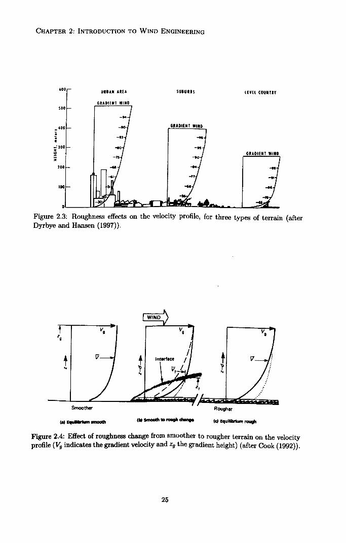
in Table 2.1 for different types of terrain. Figure 2.3 shows the effects of the roughness
height on the velocity profile for three different terrains.
Surface roughness has an influence on the velocity profile. Consider two terrains of
different roughness height, a smoother and a rougher terrain. The wind flow will be
slowed down more over the rougher terrain due to the larger surface shear stress. If
a change in roughness length is now considered over a terrain as shown in Figure 2.4,
the flow, initially in equilibrium, will reach a "new" equilibrium by the action of the
Reynolds stress. That is, the momentum required to overcome the surface shear stress
exactly balances the momentum supplied (Cook, 1992).
24
CHAPTER 2: INTRODUCTION TO WIND ENGINEERING
E
S u
S
Figure 2.3: Roughness effects on the velocity profile, for three types of terrain (after Dyrbye and Hansen (1997)).
la) Equilibrillm o^ h (W Smooth to rough diangs (U Equilibrium rough
Figure 2.4: Effect of roughness change from smoother to rougher terrain on the velocity profile (V9 indicates the gradient velocity and z9 the gradient height) (after Cook (1992)).
25
Smoother Rougher

CHAPTER 2: INTRODUCTION TO WIND ENGINEERING
2.1.5 Atmospheric turbulence
Vortex stretching and energy cascade
Visualization of turbulence shows rotational flow structures, called eddies. The rota-
tional nature of turbulent flows can be characterized by the vorticity, which can be
described as the curl of the velocity: w=Vx ii 1, and is equal to twice the rate of rota-
tion of the fluid (Pope, 2000). The largest turbulent eddies interact with the smaller ones
and extract energy from the mean flow by a process called vortex stretching, illustrated
in Figure 2.5. The larger eddies are dominated by inertia effects and viscous effects
are negligible. It follows that the angular momentum is conserved and the vorticity in-
creases, leading to vortex stretching: as shown in the figure, the vortex line increases in
length but decreases in diameter, leading ultimately to the formation of smaller eddies.
Thus, energy is transferred from large scales to smaller scales. Ultimately, the kinetic
energy associated with the smallest eddies is dissipated and converted to thermal inter-
nal energy. The whole process is called the energy cascade (Versteeg and Malalasekera,
2007). The smallest scales are characterized by the Kolmogorov length scale, defined as:
vg ) 1/4
71=(E (2.1.17)
where v is the kinematic viscosity, and f is the dissipation rate of the turbulent kinetic
energy. The large scales, are characterized by the geometry. Sometimes, the smaller
eddies can in turn contribute to larger eddies, i. e. transfer energy to the larger eddies;
this process is known as backscatter.
As larger eddies are believed to be dominated by inertia effects and extract energy from
the mean flow, their structure is anisotropic and influenced by the boundary conditions.
In contrast, the smallest eddies that are principally affected by energy dissipation, behave
in a more isotropic manner. The behaviour of smallest eddies can be considered more
universal, less dependent on the boundary conditions (Kolmogorov, 1941). /_ 8v 8u
W T. - ox 37. TV
26

CHAPTER 2: INTRODUCTION TO WIND ENGINEERING
u' jQ
A(
ti
0
10
A t2 t3
t4 t5 to
Figure 2.5: Illustration of vortex stretching (cause of the energy cascade): stretching of a vortex, to the point where two smaller vortices are formed (after Baldyga and Bourne (1984)).
Mathematical model and governing equations
The ABL is characterized by high Reynolds numbers (Re), which means that inertia
effects dominate viscous effects. The Reynolds number is defined as:
iL Re= - v
(2.1.18)
where ü and L are characteristic velocity and length scale of the mean flow and v is the
kinematic viscosity defined as:
V= F2/P (2.1.19)
where p is the dynamic viscosity and p the fluid density.
One method of describing turbulence is to consider the wind velocity to be written as
the sum of mean components v., v, w and fluctuating components u', v', w'.
27

CHAPTER 2: INTRODUCTION TO WIND ENGINEERING
u(t) ii + u'(t)
v(t) _+ v'(t) (2.1.20)
w(t) w+ w'(t)
where du' = 0. The mean value in time of each fluctuating = 0, d" =0 and dw'
-Cff
component equals zero by definition. Other variables, such as pressure, can be described
similarly.
Writing the velocity as the sum of a mean and a fluctuating components leads to extra
terms, known as the Reynolds stresses, -puý, uj, in the Navier-Stokes Equations (2.1.6
and 2.1.7). The new set of equations is known as the Reynolds Averaged Navier-Stokes
formulation (BANS):
aý aý aý __ _1
aý 82ý _1a
,2 ap%v, a_, w, T +("aX+vay+waz) pax+ýaX p+ ay az
(2.1.21)
ov _au _&J Ow 1 op 02: U _1
Op 5 apiTa- ap%, at+(Ux+uäy+uaz Päy+vax; P ax + ay + az
(2.1.22)
_ a W--
äx äy äz - (2.1.23)
In total, six extra terms are added to the Navier-Stokes equations, namely three normal
stresses: ru� Trvv Tww = -Pw'2 and three shear stresses: Tu,, _ -PU,
T�w =- pules?, r,,,,, =- pv7u?. The fact that six extra terms are added while no extra
equation is added to the system is called the closure problem. The next chapter details
the turbulence models and how they have been proposed to solve this closure issue in
order to numerically solve the equations for the flow.
28

CHAPTER 2: INTRODUCTION TO WIND ENGINEERING
2.1.6 Turbulence intensity, Reynolds stresses and length scales
Turbulence intensity and gust wind speed factor
Turbulence in the ABL can be quantified by the turbulence intensity:
1/3(vý'? +v'v' =ww
1=U (2.1.24)
where U= U2 + U2 + UZ 2. It gives a general idea of the level of turbulence in the
boundary layer, but is not enough to characterize and define the turbulent structures as
it treats the three velocity fluctuations with equal weight.
The turbulence in the wind can also be characterised by the gust wind speed factor, G,
defined as:
G_ Ugust
Uhourly
It characterises the peak wind speed in a given time interval, over the mean hourly
mean wind speed. It is a function of the turbulence intensity and it also depends on the
duration of the gust: the larger the time interval, the smaller the gust factor is.
Reynolds stresses distribution in the ABL
The distribution of the Reynolds stresses in a boundary layer is plotted in Figure 2.6.
Only the normal stresses and the shear stress -u'w' are plotted as the other shear
stresses are assumed to be negligible (those stresses are identically zero if the mean flow
is two-dimensional).
Full scale measurements have allowed expressions to be derived for the Reynolds stresses
in the ABL; the following definition of the standard deviations of the velocity are taken
from ESDU 85020 (1985, revised in 1990). The standard deviations are directly related
to the normal Reynolds stresses by: ru. = -Paüu, Tvv = -PQZ� and T,,,,,, _ -pQ2
Qu 7.5rß(0.538 + 0.09 ln(z/zo))P
U" = T+ 0.156 1n(u, /(f zo))
(2.1.25)
29

CHAPTER 2: INTRODUCTION TO WIND ENGINEERING
Figure 2.6: Reynolds stresses distribution in a boundary layer (after Pope (2000).
where
17=1 - 6fz/u� andp=q16
and au"
=1-0.22 cos4 (2h ) (2.1.26)
and
'=1-0.45 cos4 (2'rZ h) (2.1.27)
u
Figure 2.7 shows a plot of the normal Reynolds stresses, as defined by ESDU. The shear
stress has also been defined by ESDU as: 'r-, = -PVT = pu2, (1 - z/h)2.
Length scales of the velocity fluctuations in the ABL
The average size of the eddies in the flow is characterized by the nine integral length
scales of turbulence, for the three main directions, and for the longitudinal, transverse
and vertical components of the fluctuating velocity. For example, the integral length
scale in the x-direction associated with the longitudinal component of the velocity is
30

CHAPTER 2: INTRODUCTION TO WIND ENGINEERING
Figure 2.7: Reynolds stresses distribi (1985, revised in 1990) for zo = 0.01 M.
defined as:
)U 85020
°O R, ý Lx =12f u(x)dx (2.1.28)
where R.. is the cross-covariance function of the longitudinal velocity component u.
In the same manner, the integral length scales in the vertical (z) and horizontal (y)
direction of the longitudinal component of the velocity are defined as:
I fRuu(z)dz = (2.1.29)
1 °O Lü =2
jRi. iu(Y)dv (2.1.30)
Integral length scales in the x, y, z-directions are also defined for the other two compo-
nents of the velocity3, v and w.
The longitudinal integral length scales for an equilibrium boundary layer are defined in
the technical report ESDU 85020 (1985, revised in 1990). The definition of these length
scales are derived from the Von Karman spectrum for Suu, defined in Equation (2.1.38).
2p is defined is Appendix D. 'In this Chapter, the three components of the velocity are noted u, v and w. In Chapter 6, the
notation ux, uy and u. is used to be consistent with the indices used in the variables of the synthetic turbulent inflow generator.
31

CHAPTER 2: INTRODUCTION TO WIND ENGINEERING
_ A3/2(, T u/U*)3z Lu
2.5K3/2(1 - z/h)2(1 + 5.75z/h) (2.1.31)
where
A=0.115 [1 + 0.315(1 - z/h)6] 2/3
KK = 0.19 - (0.19 - Ko) exp -B(z/h)N
Ko = 0.39 B= 24R8'55 R, 00-11 ,
and Ro is the non-dimensional surface Rossby number:
. R0 u
fzo
The other longitudinal integral length scales (for the other two components of the ve-
locity) are defined in ESDU 85020 (1985, revised in 1990):
L"=0.5Iü 3 (2.1.32)
Lý =0.5
(mow )3 (2.1.33)
u\ u/
The vertical and horizontal integral length scales were first defined by Counihan (1975) as
being roughly: Lü = 0.5 Lu, and Lü = 13 Lu, which was later refined by Duchene-Marullaz
(1980) and cited in Simiu and Scanlan (1986): Lü =6/, and Lü = 0.2Lä.
A later publication, ESDU 86010 (1986, revised in 2001) redefined the vertical and hor-
izontal integral length scales based on more recent full scale measurements. They are
32

CHAPTER 2: INTRODUCTION TO WIND ENGINEERING
ý
E m m
c m J
Lx u
Lx
Lz
LY
---Lr
L'
--- Lz
150-
00-
------------------------------ 50
00 100 200 300 400 fi(X1 an
z (m) 0
Figure 2.8: Integral length scales, zo = 0.01 in, ü= 10 m/s at zref = 10 m (after ESDU 85020 (1985, revised in 1990)).
all expressed as a function of Lu:
z " = 0.5 (0.34exp (-35(z/h)(1/7))) (2.1.34) L Lx
y L2 Lz
= 0.16 + 0.68k u
(2.1.35) u
Lv Lü o,,, Lx
u =2u x
u (2.1.36)
Lw _
Lv ýv (2.1.37) Lu Lxau
The main integral length scales are plotted for a given roughness height, and a given
mean velocity in Figure 2.8.
33

CHAPTER 2: INTRODUCTION TO WIND ENGINEERING
-6 'S B
Z4
13
2
I
0
Low L4. a 3' *=PON" empomm
2
10'1 IO'' 10'' 1 10 102 I(P j [cycles/hour]
Figure 2.9: van der Hoven Spectrum of longitudinal wind speed (after Neammanee et al. (2007)).
2.1.7 Wind spectra
The van der Hoven spectrum
The van der Hoven wind spectrum characterizes the power spectral density of the wind
on a large time scale for temperate latitudes. It was first presented by Panofsky and van
der Hoven (1955) and then later developed by van der Hoven (1957). Figure 2.9 shows
the power spectral density as a function of the frequency expressed in cycles/hour.
The van der Hoven spectrum highlights three main zones (Cook, 1992):
Zone (1) shows an important peak at a low frequency of 0.01 cycles/hour. It corre-
sponds to the typical 4-day transit period of a fully developed weather system
usually called the macrometeorological peak.
Zone (2) is the spectral gap [1-10 cycles/hour] where there are very few wind fluctua-
tions, between the two majors peaks. The importance of this spectral gap is that
it allows interactions between wind climate and boundary layer to be neglected,
and thus be treated separately.
Zone (3) shows a second important peak, called the micrometeorological peak, occurs
at higher frequencies [? 10 cycles/hour] and is associated with the turbulence of
the ABL.
34
CHAPTER 2: INTRODUCTION TO WIND ENGINEERING
A more recent work, presenting full scale long term wind speed monitoring, confirmed
the existence of the spectral gap (Harris, 2008).
Since the fundamental frequencies of vibration of most buildings are higher than the
lower end of the spectral gap, turbulence is most important in wind engineering. There-
fore, when investigating wind loading on buildings, the focus is on the micrometeoro-
logical peak.
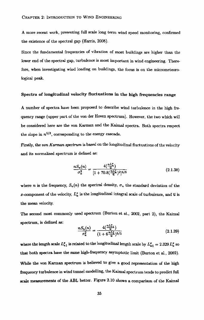
Spectra of longitudinal velocity fluctuations in the high frequencies range
A number of spectra have been proposed to describe wind turbulence in the high fre-
quency range (upper part of the von der Hoven spectrum). However, the two which will
be considered here are the von Karman and the Kaimal spectra. Both spectra respect
the slope in n5/3, corresponding to the energy cascade.
Firstly, the von Karman spectrum is based on the longitudinal fluctuations of the velocity
and its normalised spectrum is defined as:
nS,, (n) (2.1.38)
0, ü [1 + 70.8("02]5/6
where n is the frequency, Su(n) the spectral density, o the standard deviation of the
x-component of the velocity, Lü is the longitudinal integral scale of turbulence, and :9 is
the mean velocity.
The second most commonly used spectrum (Burton et al., 2002, part 2), the Kaimal
spectrum, is defined as: nSu(n)
= 4(2--1)
O, ä (1 + 6ýº)5I3 (2.1.39)
U
where the length scale Lü1 is related to the longitudinal length scale by Lü1 = 2.329 Lü so
that both spectra have the same high-frequency asymptotic limit (Burton et al., 2002).
While the von Karman spectrum is believed to give a good representation of the high
frequency turbulence in wind tunnel modelling, the Kaireal spectrum tends to predict full
scale measurements of the ABL better. Figure 2.10 shows a comparison of the Kaimal
35

CHAPTER 2: INTRODUCTION TO WIND ENGINEERING
0.001 0.01 0.1 1 Requawy (Hz)
Figure 2.10: Wind spectra over rough terrain (zo = 0.1 m) at 10 m/s at z= 30 m (after Burton et al. (2002)).
and Von Karman normalised spectra of the wind velocity over a rough terrain; these
spectra are plotted along side the spectra used in the Eurocode (European standard
code of practise) and in the Danish Standards (DS).
Cross spectrum of longitudinal velocity fluctuations
This section presents results of correlations of wind speed between two points, Pl (yi, z1)
and P2(y2, z2), separated by a distance fir. The degree of correlation between two points
is expressed by the Coherence function and can be expressed as a decaying exponential
function:
Coh(r, n) = e-f (2.1.40)
where f- n[CC (xl - Z2)2 + CC (y,
- Y2)21112
0.5 [U(xi) +(x2)]
and the constants C, z and Cy are determined empirically and depend on the roughness
height, and the mean velocity (Simiu and Scanlan, 1986). Figure 2.11 shows an example
of equation (2.1.40) for a given velocity, on which depend the constants.
36

CHAPTER 2: INTRODUCTION TO WIND ENGINEERING
1.0
40 0
0.8 °o eo C, y = 3.5
ö r° U00) = 20.8 m/sec °o N 0.6 0
p °o
0 9%O
p0 ö 0.4 ° Vvv
°o v° o
0.2 vo v
0 0.1 0.2 0.3 0.4
n(i y, -Y21)/U(10) Run 118
Y, Yz (meters)
o0 12 a0 35 0 12 35
v 80 35
Figure 2.11: Coherence functions (after Simiu and Scanlan (1986)).
The cross spectrum Su u2 can be deduced from the Coherence function:
1Sü . u2I I= Coh(r, n) S(zl, n)S(z2i n)
where S(zi, n) and S(z2, n) are the spectra of the longitudinal velocity fluctuations at
points Pl and P2.
2.2 Response of tall buildings to wind loading
2.2.1 Introduction: building aerodynamics
The domain of wind engineering is concerned with the interactions between the At-
mospheric Boundary Layer and buildings, which are typically bluff -bodies. This study
37

CHAPTER 2: INTRODUCTION TO WIND ENGINEERING
Wind direction
Figure 2.12: Air flow pattern around a building, side view.
focuses on tall buildings and the aerodynamics of these structures are presented in this
section. The Council on Tall Buildings and Urban Habitat (CTBUH) keeps a record
of all existing and future tall buildings and set the following criterion to enter their
database: 14 or more storeys and over 50 meters.
Figure 2.12 represents the streamlines of the air flow around a building when the incident
wind is normal to the building.
On the windward face of the building, at about two-thirds of the height, the flow comes
to rest at the stagnation point (F), where the pressure is maximal. Below F, the flow goes
down and allows recirculation vortices to develop near the ground. For tall buildings,
this vortex creates high downward wind velocity that can severely affect the comfort of
pedestrians walking around the structure.
Above F, the flow goes up to the top of the building. On the windward edge of the roof,
the flow is separated (S), and a separation bubble appears. Reattachment can occur on
the roof. Pressure distributions on the roof show high suction (negative pressures) near
the windward edge. Pressures become less negative as the flow goes to the leeward edge.
The leeward face is characterized by negative pressures that are relatively constant. In
fact, the building is subjected, on average, to negative pressure on all its faces, except
the windward face.
When seen from the top, the flow also separates at the right and left edges of the building.
38

CHAPTER 2: INTRODUCTION TO WIND ENGINEERING
Figure 2.13: horseshoe vortex after Cook (1992): Figment-
slab building model in boundary layer mean velocity profile. on of
Just after the edges, there is a formation of vortices. Then, the flow reattaches if the
building is long enough in the along-wind direction. If the building is shorter, the flow
does not reattach on the side of the building. The two branches of the flow that have
been separated join in the wake, downstream of the structure. Recirculating vortices
form near the base of the building, and the flow detaches and envelop these recirculating
vortices. forming the horse-shoe vortex, Figure 2.13.
Just downstream of the structure, recirculating vortices develop and the flow can reat-
tach through different patterns: studies on the flow behind a rectangular feature have
shown that as the Reynolds number increases, the wake is first separated following a
symmetrical pattern and then, for Re > 30, starts oscillating; this is called the vortex
shedding (Cook, 1992). The symmetrical flow pattern and vortex shedding are illus-
trated in Figure 2.14. The Strouhal number St, non-dimensional, helps to characterise
this phenomenon.
St =nD (2.2.1)
39

CHAPTER 2: INTRODUCTION TO WIND ENGINEERING
Symmetrical wake
Vortex Shedding
Figure 2.14: Symmetrical wake for 5< Re < 40 and Vortex shedding past a rectangular cylinder (laminar votex street for 40 < Re < 200, view from the top.
Figure 2.15: Vortex-formation model showing entrainment flows (after Gerrard (1966)).
with n, being the frequency of a full cycle of vortex shedding, Da characteristic di-
mension of the body in the normal direction of the flow, and v,, the velocity of the
oncoming wind flow. Okajima (1982) showed the dependence of the Strouhal number
with the width to height ratio of rectangular cylinder as well as its dependence with the
Reynolds number.
The formation of vortices in the wake has been extensively described by Gerrard (1966)
for a circular cylinder and is illustrated in Figure 2.15. On this figure, the instantaneous
flow line pattern shows how the flow is separated and two shear layers appear on both
sides of the cylinder. The flow (a) is then entrained into the growing vortex, (b) goes into
the developing shear layer and (c) is captured in the near wake region. Vortex shedding
is therefore the result of the interaction of the two shear layers (Bearman, 1984).
The main difference in the flow around sharp-edged bluff-bodies and circular cylinders
is the location of flow separation: for a circular cylinder, there is a critical Reynolds
40

CHAPTER 2: INTRODUCTION TO WIND ENGINEERING
number range, for which the two separation points on the sides of the cylinder are not
fixed and oscillate between the front and the back of the cylinder. In the subcritical
range, for 300 < Re <3x 10⁵, the wake is completely turbulent, but the boundary layer
separation is still laminar. In the critical range, 3x 10,9 < Re < 3.5 x 10⁵, the separation
is laminar on one side and turbulent on the other side but the boundary layer remain
laminar. For higher Reynolds numbers, up until 1.5 x 10⁶, the separation is turbulent,
but the boundary layer is partly turbulent, partly laminar. For even higher Reynolds
numbers, the boundary layer is completely turbulent at one side, and for Re >4x 10⁶,
it is turbulent at two sides. This transition from laminar boundary layer with a laminar
boundary layer separation to a turbulent boundary layer with turbulent boundary layer
separation does not occur for a sharp-edged bluff-body, as separation must occur at the
front edges of the structure.
Bearman (1984) pointed out that vortex shedding is likely to occur for structures with
a high aspect ratio (height/width). Consequently, the excitation induced by vortex
shedding is particularly important and will be detailed in section 2.2.2.
If the incident wind is not normal to the building, which is mostly the case, another
aerodynamic feature is of importance: the delta-wing vortex. This conical vortex de-
velops at upwind corners, when the flow separating from an edge has a component of
velocity along the line of separation (Sachs, 1978). In the centre of these vortices, the
suction is large, possibly leading to structural severe damage. Recirculating vortices
develop along the edge, downstream the Delta-wing vortices, as shown in Figure 2.16.
2.2.2 Aeroelastic phenomena
The study of the flow around buildings shows that this is a fundamentally three-
dimensional field: the air flow diverges in both cross-wind directions and in the vertical
direction on the roof. This section aims to describe the main aeroelastic phenomena,
vortex shedding, buffeting, and galloping excitations that can occur for structures.
41

CHAPTER 2: INTRODUCTION TO WIND ENGINEERING
Figure 2.16: Incident flow not normal to the building: the Delta wing vortices.
9
Wind
Figure 2.17: Wind response directions (after Mendis et al. (2007)).
42

CHAPTER 2: INTRODUCTION TO WIND ENGINEERING
Vortex shedding excitation of a flexible structure
The most important aerodynamic feature when studying flow around a building, espe-
cially tall buildings, is vortex shedding. Vortex shedding can induce oscillations in the
direction transverse to that of the incident wind for flexible structures.
For bluff-bodies, the Strouhal number, St, depends on the structure shape and is approx-
imately constant for high Reynolds numbers (Re > 103). As a consequence, knowing
the natural frequency of the building f,,, as well as St and the across-wind dimension of
the structure, D, leads to the definition of the critical wind velocity u, = "D, for which
the frequency of the vortex shedding equals the natural frequency of the building. This
is only valid as long as the vortex shedding remains a regular (single frequency) phe-
nomenon. In the super-critical range of Reynolds number (3 x 10⁵ < Re <3x 10⁶), the
vortex shedding becomes random and is characterized by unsteady disorganised wake
motion, and the vortex excitation becomes random. The amplitudes of the oscillations
are lower than those seen at one of the natural frequencies of the building. Wind gusts
make the occurrence of single-frequency vortex excitation more difficult because of its
multi-directional and unsteady characteristics (Sachs, 1978; Simiu and Scanlan, 1986).
If the structure can move in response to the vortex shedding excitation, a major aeroe-
lastic phenomenon can occur: the "lock-in". As the velocity increases, the frequency
of vortex shedding f�9 increases proportionately to the shedding frequency of a static
cylinder, given by the Strouhal number. When the vortex shedding frequency is close
to the natural frequency fa of the building in the transverse direction, the amplitude of
the response increases, and the building oscillates at the vortex shedding frequency. As
the velocity increases, the frequency of the vortex shedding is locked on to the natural
frequency of the building, and the amplitude of the building response is maximal. At
this point, the building "controls" the vortex shedding frequency, hence the "lock-in"
phenomenon. If the velocity increases further, the amplitude of the oscillations drops,
and at the upper end of this range, the vortex shedding frequency reverts to that of a
static cylinder.
43

CHAPTER 2: INTRODUCTION TO WIND ENGINEERING
'u
31 , 4-2A
is
L
13
03
0.1 10
U*
Figure 2.18: Free vibration of a cylinder: response frequency vs reduced flow speed, lock-in phenomenon identified for f`1.4 (Williamson and Govardhan, 2008).
While there is an extensive literature about vortex induced vibrations of elastically
mounted cylinders (Williamson and Govardhan, 2008), illustrating the lock-in phenom-
ena, little has been done for more complex structures, such as a flexible cantilever. Figure
2.18 illustrates the response frequency versus the oncoming flow speed, and the lock-in
phenomena is clearly identified: below the natural frequency of the building (f' < 1.0),
the building oscillates at the vortex shedding frequency with small amplitude, but as
the flow speed increases, increasing the vortex shedding frequency, the frequency gets
closer to the natural frequency of the building, and the cylinder starts controlling the
vortex shedding frequency.
A wind-tunnel study of an oscillating tall building has been carried out by Fediw et al.
(1995). It was found that for a velocity below the critical velocity (previously defined),
the vortex formation is controlled by the building motion. It was confirmed that for
a velocity close to the critical velocity, the natural shedding frequency coincides with
the driving frequency and the largest shedding forces are observed. For velocities larger
than the critical velocity, the motion effects are small and natural shedding is stronger.
In addition, the local Strouhal number was found to decrease with height, probably due
to the log-law velocity profile.
44

CHAPTER 2: INTRODUCTION TO WIND ENGINEERING
Buffeting excitations
Buffeting excitation of a building is caused by the combination of the velocity fluc-
tuations of the oncoming wind flow and the turbulence shed in the wake of an up-
stream building. Buffeting creates along-wind loading on a building but the presence of
three-dimensional excitations due to upstream buildings might also induce a torsional re-
sponse. Tall buildings are more likely to undergo buffeting as their rather lower damping
and light weight imply lower natural frequencies, that are more likely to be in the same
range as the average frequency of occurrence of powerful gusts (Simiu and Scanlan,
1986). But even if the building's natural frequency does not lie in the range of the
wind gusts, buffeting excitation can be caused by simply wake effects from neighbour-
ing buildings. Regular vortex shedding might occur from neighbouring buildings and
cause along-wind regular oscillating loading, possibly at a frequency close to the natural
frequency of the building.
Within best-practise codes, extreme wind loads due to buffeting are predicted using
gust factors, which are factors that characterize the fluctuating component of the wind
velocity. However, it does not predict the dynamic response and it has been observed
that this does not lead to accurate predictions when there are upstream buildings. When
the dynamic response of a building is significant, wind tunnel tests are carried out either
with an aeroelastic model, or a static combined to a high frequency force balance.
2.2.3 Structural dynamics
Unlike low and medium-rise buildings that are more or less stiff structures, tall buildings
are more flexible and have lower natural frequencies, which makes them subject to vortex
and gust excitation in addition to static deflections.
Nature of forces due to wind loading
For a single-degree of freedom system (SDOF), the equation of motion is determined by
equating the oscillating forces:
45

CHAPTER 2: INTRODUCTION TO WIND ENGINEERING
my +4+ ky = F(t) (2.2.2)
where y is the displacement of the structure m the mass per unit span, ca viscous-type
damping term, k the stiffness, and F(t) the time-dependent force due to wind loading.
The natural angular frequency of the system is given by w,, = k/m and the natural
frequency by f,, = w,, /(21r). The damping ratio is ýn = c/(2 km) where 2 km is the
critical damping coefficient, above which the response is non-oscillatory.
The total dynamic response of a lightly damped structure to any excitation can be
written as the superposition of the individual modal responses. The response in each
mode is concentrated at a single frequency, called the modal frequency. Therefore, for
analysing purposes, the whole structure is viewed as a set of independent single-degree
of freedom systems, each corresponding to a single mode (Cook, 1992). Each modal
response corresponds to:
(i) A modal deflection, which is the deflection at the position of maximum amplitude.
(ii) A mode shape, defined as the ratio of the local deflection and the modal deflection.
Usually, the first three modes appear in the dynamic response of a building. They are
identified by peaks in the power spectral density of the acceleration response. The first
two modes correspond to motion in the two principal horizontal directions, the third
mode corresponds to the torsional response.
In wind engineering, as stated by Davenport (1995), the three sources of aerodynamic
excitation causing dynamic response are:
1. Single-frequency excitation: forces caused by vortices shed in the wake
of the structure, affecting primarily the resonant responses and occuring
primarily in the cross-wind direction.
2. Random excitation: forces due to the turbulent fluctuations (or "gusti-
ness") of the oncoming wind flow, causing both background and reso-
46

CHAPTER 2: INTRODUCTION TO WIND ENGINEERING
nant responses in the along-wind and cross-wind directions.
3. Forces induced by the motion of the structure, such as aerodynamic
damping forces which control the resonant response amplitude.
Single-frequency vortex excitation
If any random excitation is artificially excluded and the sole response to a single fre-
quency excitation is studied, F(t) can be written as a simple sinusoidal function: the
total force acting on the structure is defined as F= FO cos wt.
The solution can then simply be expressed as the sum of the transient and steady-state
solutions. The transient solution creates the decaying exponential envelope dependent
on the initial disturbance, and the steady-state solution is a sinusoidal function, which is
dependent on the excitation force. The steady-state response of a SDOF can be written
as:
x(t) = FOH(w) cos(wt - 0)
where 2ýn (w/wn)
=tan 1
and H(w) is the mechanical magnification factor (or structural admittance) and defined
as: 1
H(w) _ (2.2.3) k (1- (w/Wn)2)2 + 4£n(wIwn)2
The amplitude of the response is characterized by the amplification factor, which is
the ratio between the amplitude of the response to the harmonic loading xf and the
amplitude of the response to a constant load xo (static load): x f/xo. The amplification
factor decreases as the damping ratio increases4.
If the frequency of the excitation force, f, reaches the natural frequency of the structure,
f,,, the amplitude of the oscillating steady-state solution increases to a constant level,
which can be dangerous for the structure, and resonance occurs. If the exciting frequency
4This will be illustrated in section 5.3.2 and in Figure 5.5.
47

CHAPTER 2: INTRODUCTION TO WIND ENGINEERING
does not approach the natural frequency, as in most cases, the steady-state solution is
negligible.
Random excitation: turbulence in the oncoming wind flow
The dynamic response to a random frequency excitation, such as turbulent fluctuations
in the oncoming wind flow, can no longer be expressed in terms of the oscillation am-
plitude and phase. Instead, a statistical approach is chosen, and was first introduced
by Davenport (1961). The velocity fluctuations of the wind are characterized by their
power spectral density (PSD) Su(n) (n is the frequency) of the wind spectrum, from
which the PSD of F can be defined Sf(n).
The response to this random excitation comprises the response to both the mean wind
load, and the random component of the wind load. The former corresponds to the
response to the dynamic head (q =2 pCDV where p is the air density, CD the coefficient
of drag and V the wind velocity) and the latter remains the sum of transient and
steady-state components. However, the shape of the steady-state response is no longer
sinusoidal, since it depends on a random parameter, the excitation force. As for the
response to a simple oscillating excitation force, there will be a resonant response and a
non-resonant response to random excitations.
The method developed by Davenport (1961) allows the response of the structure to the
wind gusts to be determined in the frequency domain: the method is the wind loading
chain. The wind is described in the frequency domain by the wind gust spectrum. The
one used by Davenport is as follows:
nS�(n) _2
nLü/; g
Qü 3 (1 + (nLü/ 1)2)4/3
but in theory any spectrum model may be used, such as the one described in section
2.1.7. Only the spectrum of the longitudinal velocity is considered as it is where most
of the energy is contained. The wind spectrum is then filtered by the aerodynamic
admittance X0(n), which takes into the account the fact that the typical structure
48

CHAPTER 2: INTRODUCTION TO WIND ENGINEERING
1 C 0
C
U C
0.1
U E cc C
a 0.01 nb U
0.001 0.01 0.1 1 Figure 2.19: Aerodynamic admittance function (after Houghton and Carruthers (1976)).
is not point-like and velocity fluctuations approaching the windward face cannot be
assumed to be uniform. This implies that the pressures acting on the building will
generally not be correlated, especially at high frequencies. Effectively, that means that
the aerodynamic admittance acts as a low-pass filter. An example of an aerodynamic
admittance is shown in Figure 2.19. It can be observed that it is closed to 1 in the
low frequencies and decreases as the frequency increases, this expresses that the large
gusts that envelop the structure have more effect on the building than the smaller gusts
(higher frequencies).
The aerodynamic admittance function then produces a force spectrum Sf, related to
the velocity spectrum through the aerodynamic admittance:
Spe) . 41Xa(n)I2Sti(2 )
ü
The response spectrum is then obtained by filtering the force spectrum with the struc-
tural admittance (similar to the structural admittance defined in Equation (2.2.3)). The
response spectrum presents peaks corresponding to the background response at a lower
frequency, and may also exhibit a peak at a higher frequency corresponding to the
resonant response.
49

CHAPTER 2: INTRODUCTION TO WIND ENGINEERING
s) WAKE FORCES Fw
tafwlt)ýý's
TURVAIENC( INTENSITY,
LOW
MICH
M /U (re/Ulis Figure 2.20: Spectra of forces due to the fluctuations in the wind (A), and spectra of forces due to vortices shed in the wake (B) (after Davenport (1995)).
Summary of wind forces acting on the building
To sum-up, the response of the structure is composed of the background response and
the resonant response with a well defined frequency, generally higher than the peak for
the background response. The background response consists of "an irregular and slowly
varying component" and is larger in the along-wind direction than in the cross wind
direction (Davenport, 1995).
The forces due to single frequency excitations (vortex shedding) and due to the fluctu-
ations in the wind are presented in the domain frequency in Figure 2.20. In the case
of forces due to the fluctuations in the oncoming flow (A), the spectra is quite broad,
but shows a larger response at smaller reduced frequencies f L/U, hence at larger wind
speeds U. In the case of wake forces, the peak of the spectra is much sharper and cor-
responds to the frequency of the vortices shed in the wake of the structure (related to
the Strouhal number of the structure). It is interesting to note that when there is more
turbulence intensity, which means more fluctuations in the wind, the forces spectra due
to the wake gets broader. It appears that the fluctuations in the wind tend to damp the
single-frequency vortex shedding excitation.
2.3 Summary and conclusions
This chapter introduced the field of wind engineering, and presented the important
features of the flow around buildings, and the main characteristics of the Atmospheric
50
A) TUR ULENCE FORCES FT

CHAPTER 2: INTRODUCTION TO WIND ENGINEERING
Boundary Layer, including the wind spectra and the integral length scales. This chapter
also introduced building aerodynamics and the main characteristics of the dynamic
response of buildings to wind loading, including the wind loading chain developed by
Davenport. It is the object of the next chapter to present the models used in CFD to
model the ABL and the flow around buildings.
51

Chapter 3
Literature Review of
Computational Wind Engineering
3.1 Introduction on Computational Wind Engineering
3.1.1 CFD in wind engineering
Computational Fluid Dynamics (CFD) provides various tools to investigate complex
fluid flows. The spatial domain is discretized into small cells to form a volume mesh. Nu-
merical methods, such as the Finite Difference Method (FDM), Finite Volume Method
(FVM) or the Finite Element Method (FEM) are then applied to reformulate the Navier-
Stokes equations (2.1.1-2.1.4) as a series of algebraic equations. These equations are
solved numerically over the domain, with specified boundary conditions to simulate the
effects of the environment.
Soon after computers first became available they were used in the solution of partial
differential equations and by the 1970s the use of computers to solve the equations gov-
erning fluid flow was under active investigation by researchers (Patankar and Spalding,
1972; Launder and Spalding, 1974). The application of CFD to wind engineering prob-
lems started in the 1980s, when a market for CFD emerged in a handful of engineering
fields and several companies like Fluent, AEA Technology and Computational Dynam-
52

CHAPTER 3: LITERATURE REVIEW OF COMPUTATIONAL WIND ENGINEERING
ics emerged to fulfil this need. Despite progress of Computational Wind Engineering
(CWE) in this time, wind loading standards and building codes of practice still rely
on wind tunnel studies for non-standard building designs. However the use of wind
tunnels is associated with several limitations that CFD can potentially overcome. For
example, it is not possible to fully model swirling flow impacts on structures and gust
fronts in wind-tunnels. Furthermore, modelling of flow inside buildings or around bluff
bodies in wind-tunnels is difficult due to Reynolds number limitations (Stathopoulos,
1997). CFD offers some flexibility that is maybe of a different nature than the flexibility
offered by wind-tunnels. In addition to flexibility, it is possible with CFD to extract
data everywhere in the domain. But perhaps the most prominent advantage of CFD in
wind engineering is the fact that it can potentially be integrated into the virtual design
process of a building.
However, despite these potential advantages of CFD, it has been the target of many
critics from the wind engineering community, for whom CFD is a very young tool that
cannot compare with wind tunnels and the level of expertise reached in wind tunnel
testing. Some of these criticisms are based on the fact that on some occasions, CFD users
have provided different solutions, sometimes simply wrong, to the same problem (often
claiming to use the same models) (Richards and Quinn, 2002; Sabatino et al., 2010).
Wind tunnel testing requires an experienced worker who knows the characteristics of
the wind tunnel, the type of flow it can produce and the type of the flow that needs
to be modelled. In the same way CFD requires an experienced user who knows what
equations are solved, and how, and the details of the models used. Because wind tunnels
have been used for much longer, very precise guidance exists; the same cannot be said
about CFD, although there has been attempts to provide better and unified guidance
for the application of CFD to wind engineering such as in Franke et al. (2004,2007).
As recognized by Castro and Graham (1999), many of the models have been developed
for very precise applications by researchers concentrating on modelling a particular flow,
often in the aeronautics industry, concerned with flows around streamlined bodies. These
CFD codes might be very good at predicting the flow for a certain application but would
53

CHAPTER 3: LITERATURE REVIEW OF COMPUTATIONAL WIND ENGINEERING
fail to offer a more general code simply because they were not designed for a general use;
this is true of most turbulent models, which have been designed for specific applications.
Turbulence modelling is particularly important in CWE because unlike the aeronautics
industry that models flows around streamlined bodies, CWE is concerned with flows
around bluff bodies. For this reason, there is a need for assessing the performance of
each of these models in CWE.
However over the past 10 years, much progress has been made in CFD for wind engineer-
ing problems, to the point where its use has been accepted for some applications. This
includes predicting wind speeds in pedestrian areas, where CFD is considered a good
substitute to wind tunnel testing, as reported by Bitsuamlak and Simiu (2010) at a re-
cent symposium on CWE. Bitsuamlak and Simiu reviewed the areas in which CFD had
proven its use, and among these, it was noted that CFD could be useful to predict global
aerodynamic loads on structural elements, or could complement experimental data on
flow generation. In short, far from being redundant in the field of wind engineering, or
providing a complete alternative to traditional wind tunnel testing, CFD is best used in
conjunction with wind tunnels to achieve a better understanding of wind flow around
buildings and wind loads on structures.
It could be said that the major disadvantage of CFD in wind engineering is its apparent
ease of use and approachability. However, CFD does requires very careful attention to
the following aspects: the discretization of the domain (mesh), turbulence modelling
and boundary conditions as stated by Castro and Graham (1999). The purpose of this
chapter is to review the current state of the art in CWE, and more precisely in these
three areas of interest.
3.1.2 CFD methodology
Four steps can be distinguished in the CFD process:
9 Geometry: The domain and the structure within that domain are built at this
step. Details on how the geometry of the domain and the structure should be
54

CHAPTER 3: LITERATURE REVIEW OF COMPUTATIONAL WIND ENGINEERING
determined are given in the present Chapter.
" Meshing: At this key stage, the spatial domain is divided into Control Volumes
(CV) to form a mesh (grid. ) Guidelines for this are presented in section (3.1.4).
" Model set-up: Boundary conditions, turbulence model, material properties, solver
settings, data output options, frequency of the output of the flow field, etc are
chosen at this stage. This Chapter explains how the boundary conditions should
be chosen in CWE. As the choice of the turbulence model is crucial, two sections are
devoted to this issue: section 3.3 develops the methods for modelling turbulence
using the Reynolds Averaged Navier-Stokes equations. Section 3.4 presents the
Large Eddy Simulations (LES), which allows most of the turbulence length scales
to be resolved.
" Solver: the CFD code discretizes the Navier-Stokes equations, and solves them
over the discretized domain of interest. Details on the solver can be found in
section 3.1.3.
" Analysis of results or post-processing where data such as velocity flow fields, vor-
ticity and pressures are extracted on lines, planes, surfaces of the domain under
investigation.
3.1.3 Discretization of the governing equations
Spatial discretization
Once the governing equations of the flow, the Navier-Stokes equations, have been deter-
mined (first defined in Equations 2.1.1-2.1.4), they need to be spatially discretized since
55

CHAPTER 3: LITERATURE REVIEW OF COMPUTATIONAL WIND ENGINEERING
in general they cannot be solved analytically:
au äu au +(U +v +w
au 1 ap )+ _
lard -fV+ at äx äy äz päx päx
av av av +v +W- + (u
äv 1 ap O
)+ 107-� _ -fU+ at ay ax z 'Oy p az
aw+(u aw+aw+aw +lap+9 _-1arv, at ax öy az p az p az
app ate, apw ax+ a+ 09Z 0
That is, continuous equations must be written in a discrete form. The Navier-Stokes
equations are discretized using discretization methods such as the Finite Difference
Method (FDM), Finite Volume Method (FVM) or the Finite Element Method (FEM).
The FVM is the most commonly used in CFD codes, partly because conservation of
fluxes through a particular volume is easier to ensure with FVM, and FVM is more
efficient in terms of CPU usage. ANSYS-Fluent, which is used for the present work,
uses the FVM.
The Finite Volume Method can be described as follows: The spatial domain is divided
into finite control volumes, as shown in Figure 3.1. The discretized formulation of the
Navier-Stokes equations are then solved over the grid. The balance of mass, momentum
and energy is ensured by solving the conservative form of the Navier-Stokes equations.
The integral formulations of these equations are expressed in equation 3.1.1 for a variable
56

CHAPTER 3: LITERATURE REVIEW OF COMPUTATIONAL WIND ENGINEERING
(a) (b) Figure 3.1: Structured (a) and unstructured mesh (b). The structured mesh is com- posed exclusively of hexahedral elements, and the unstructured mesh is composed of tetrahedral elements.
apý fv 20t dV + fE pOV . dA
Rate of change Net convective
= fl; F Vq " dÄ +fV SOdV
Net diffusive Source (3.1.1)
(transient) flux flux term
where V is the volume of the CV, E is the surface of the CV p is the fluid density, v" is
the velocity vector, Ä is the surface area vector, P' is the diffusion coefficient for 0, V
is the gradient of 0, and So is the source of 0 per unit volume.
For each CV, the rate at which a variable flows in through the boundaries is calculated
and the rate of change of the variable is computed. A matrix is built with all variables in
each cell. This matrix is solved by iteration. The process is stopped when the residual
error reaches a pre-set value, which can be different for each variable.
The size of the grid cells must be carefully chosen. Generally, most cells are placed where
the gradients of the flow variables are largest. A compromise must be found between
57
CHAPTER 3: LITERATURE REVIEW OF COMPUTATIONAL WIND ENGINEERING
the number of cells of the mesh and the degree of accuracy that is required. On the
one hand, a very fine mesh with a large cells number might require large CPU time to
converge. In addition, it might also be difficult to converge because of oscillating features
of the flow at small scales. On the other hand, a very coarse mesh might not provide
accurate results by missing important features of the flow, such as a recirculation zone
on a roof.
The convection and the diffusion terms in equations 3.1.1 require the values of 0 at
the surface of the control volume. However, since only the central values are stored by
the CFD code, a scheme must be adopted to extrapolate the values on the boundaries.
Most schemes uses the upstream cell's values to compute the face value (" upstream" is
understood as upstream of the flow).
The simplest of these schemes is the first-order upwind differencing scheme which states
that the value at the surface equals the value at the centre of the upstream cell. This
method can be used when the expected level of accuracy is low. The second-order upwind
scheme uses the cell-centered value 0 and the gradient within the upstream cell 0¢ to
compute the face value Of:
Of =O+0O"r (3.1.2)
where ¢ is the cell-centered value in the upstream cell, V4 is the gradient in the upstream
cell and r is the vector from the upstream cell centroid to the face centroid.
A third major scheme is called QUICK (Quadratic Upstream Interpolation for Con-
vective Kinetics) and is a quadratic differencing method. The value at the surface of
the cell n is computed using the values at the centres of the cell immediately upstream
(n - 1), and the second cell upstream (n - 2). 1 can be written as follows:
Of =1 [AOD-1 + Bcu] +8 [COD-1 - DOD-2] (3.1.3)
where U stands for cell upstream of the surface, D-1 for the immediately downstream
58

CHAPTER 3: LITERATURE REVIEW OF COMPUTATIONAL WIND ENGINEERING
cell and D-2 for the second cell downstream. A, B, C and D depend on the grid dimen-
sions. The QUICK scheme can only be used when the grid is composed of quadrilateral
and hexahedral cells as the above equation requires a unique upstream face and a unique
downstream face.
Temporal discretization
For transient simulations, the rate of change of 0 with respect to time, Opo/öt, must
be taken into account and hence written in a discretized form. This can be done with
an implicit first-order scheme, that is, 0,, +1 is related to the value of 0�+1 in the neigh-
bouring cells. If more accuracy is required, a second-order scheme can be adopted: The
values at the current and at the previous time steps are combined to calculate the rate
of change at the future time step. The choice of the time-step is crucial as it must be
small enough to capture the important features of the flow, but not too small because a
very small time step will require much more computational power without any increase
in accuracy.
Temporal and spatial discretization are related through the Courant number:
uxAt Ox (3.1.4)
where u is the mean velocity of the flow, At is the time step, and Ax a characteristic
grid size. The time step size is chosen such as C<I. This means that the distance
travelled by a particle of fluid during one time step should not be longer than the grid
size.
Pressure-velocity coupling
Figure 3.2 summarizes the sequence of events followed by the CFD solver, for both
segregated and coupled solvers.
In a segregated solver, the governing equations are solved sequentially. Firstly, the
59

CHAPTER 3: LITERATURE REVIEW OF COMPUTATIONAL WIND ENGINEERING
momentum equations are solved with an assumed pressure gradient. The computed
solution is then put into the continuity equation because the computed velocities from
the momentum do not a priori satisfy the continuity equation, which leads to a cor-
rected pressure. This corrected pressure is then put back into the momentum equations.
This process is iterated until all the variables satisfy the momentum and the continuity
equations. The other variables (velocity, mass flux) are then updated accounting for
the new computed pressure. The scalar variables, such as turbulence quantities, are
calculated afterwards. The whole process is repeated until all variables have converged,
that is, the residuals of the variables have gone below a pre-fixed value. In addition
to the residuals, forces, mass flux and various field variables at monitor points must be
monitored to ensure that these have reached a stationary state, which means that the
variables do not vary with time, or if they do, they vary in a consistent manner that
can be predicted based on previous occurrences. One variant of this process is called
the SIMPLE (Semi-Implicit Method for Pressure-Linked Equations) scheme.
The PISO (Pressure Implicit with Splitting of Operators) method is similar to SIMPLE
but uses a second pressure correction equation before solving for the scalar variables.
Versteeg and Malalasekera (2007) remarked that neither of these methods is superior
in terms of accuracy. Their performance seems to be dependent on the application.
However, PISO is recommended for transient simulations by the ANSYS-Fluent manual,
and is, therefore, used in the present work.
For completeness, the coupled pressure-velocity method simultaneously solves the sys-
tems of momentum and pressure-based continuity equation. Consequently, the pressure
correction equation is not necessary. Due to the strong coupling, the iteration time
and memory requirements are increased compared with a segregated solver, but the
convergence, when occurring, is improved.
60

CHAPTER 3: LITERATURE REVIEW OF COMPUTATIONAL WIND ENGINEERING
Solvers Pressure-based solver
f
Segregated Coupled
Update
Solve sequentially U. V. W
Update
Solve simultaneously system of momentum and continuity equation
Solve pressure-correction (Continuity equation)
Update mass flux, pressure, and velocity
Update mass flux
Solve energy, tubulence equations
Converged ?
Figure 3.2:
3.1.4 The computational grid
Structured and unstructured grids
Solve energy, tubulence equations
Converged ?
and Solver for the flow equations.
A structured grid is defined as being composed of the regular repetition of an identifi-
able block (usually quadrilaterals in 2D, hexahedra in 3D), Figure 3.1a. Unstructured
grids are characterized by irregular patterns as shown in Figure 3.1b; information on the
location of the vertices and the connectivity to the neighbouring cells must be stored for
each cell. For a very complex geometry, it is often easier to build an unstructured grid,
while structured grids are limited to simple geometry and become either unfeasible or
not optimal in terms of CPU time and accuracy for complex geometries. Practically,
this means that for a structured grid, if the index of a node is known, the connectivity
61

CHAPTER 3: LITERATURE REVIEW OF COMPUTATIONAL WIND ENGINEERING
information of this node is also known. While for an unstructured grid, a connectivity
table detailing the connectivity for each node is needed. As far as most CFD codes
are concerned (including ANSYS-Fluent), all grids are treated as unstructured. How-
ever, in some applications the physics of the flow requires the use of a structured grid.
Besides, for a given geometry, a structured grid often involves a lot less nodes than
an unstructured grid, which means that the computational time can be significantly
reduced.
General guidelines for building the grid
Franke et al. (2004), published fairly general guidelines for good practise in CWE. No-
tably they specified how the computational grid should be defined: The grid should be
fine enough to capture vortices and shear layers, grid stretching and compression should
be avoided particularly where the gradients of values are large and numerical diffusion
must be limited, so that, ideally, the line connecting the centres of two consecutive cells
should be aligned with the flow, Figure 3.3. The numerical diffusion is related to the
orthogonality of the mesh: a mesh is defined as orthogonal if, for each face within it,
the face normal is parallel to the vector between the centres of the cells that the face
connects. An example is a mesh of hexahedral cells whose faces are aligned with a
Cartesian coordinate system. The second order differencing in Fluent tried to minimize
this.
k mom accurst. thin
Figure 3.3: Numerical Diffusion.
In terms of an element hierarchy, hexahedra are known to introduce smaller truncation
errors, so these elements are preferred to tetrahedra wherever it is feasible. Generally,
62

CHAPTER 3: LITERATURE REVIEW OF COMPUTATIONAL WIND ENGINEERING
a fine mesh should be used in the regions of high gradients. Furthermore, the following
criteria must be checked for a good quality mesh: the aspect ratio and the angle skew-
ness, as illustrated in Figure 3.4. Both are used to check the quality of a mesh composed
of hexahedra and tetrahedra (in 3D). The aspect ratio will naturally be far from 1 near
the walls, as the boundary layer requires a finer grid in the direction normal to the wall
(steep gradients) than parallel to it. The skewness is particularly important when using
tetrahedra. A third quality criteria must be checked: the stretching ratio, which can be
defined as the rate at which the cell size increases between two consecutive cells.
Aspect ratio QAR
Skewness QE
8
d b
c
Maxe e ]1 AR - Mine-l-, -e72 -
B
eB
QE = Max 0---60 60-8...... 120 60
ei = (a + c)/2 es = (6 + d)/2 Ideal
Ideal aspect ratio 171 I
QE=O O<QE<1 QAR=I QAR>I
Acceptable range: 0< QE < 0.75
Figure 3.4: Mesh quality: Aspect ratio and Skewness
Results are considered grid independent when the extrapolation of the results obtained
with gradually refined meshes reach an asymptotic range. It is recommended to test at
least three grids with increasing refinement. Grid independence is a major criterion for
good-quality results.
2D and 3D grids
A three-dimensional grid is an obvious choice as all features of the flow can only be
captured in a 3D domain. For example, vortex shedding is a transversal flow character-
63

CHAPTER 3: LITERATURE REVIEW OF COMPUTATIONAL WIND ENGINEERING
istic and buffeting is caused by 3D wind excitation. The loss of these features of flow
must be taken into consideration when a 2D grid is used. A 2D mesh is suitable for
either; 1) coarse and quick runs; or 2) when a single phenomenon is to be observed; or 3)
if certain parameters need to be tested with different values to assess their influence on
one particular feature of the flow. It is generally not suitable when modelling turbulent
structures arising from bluff body, as these are essentially 3D.
3.2 Introduction to turbulence modelling
Turbulence modelling is one of the main challenges when modelling wind flows within
the ABL. Researchers have tried to improve numerical results by developing numerous
turbulence models. They started with two-equation models, that were to be used in
steady-state simulations, commensurate with the computer capacities then available.
These models were then modified into several different versions in order to improve the
characteristics of the predicted flow. However, most of these modified versions would
in fact only improve one aspect of the flow, and would therefore be quite specific to a
particular application (Castro and Graham, 1999). Consequently, as computer resources
were increased, the use of two-equation turbulence models in academia was largely
replaced by more computationally expensive models to solve most of the turbulence
scales in a transient manner. Most prominent is the so-called Large Eddy Simulation
(LES). Nowadays, although the focus in academia is on LES, two-equation turbulence
models are still investigated as their robustness, simplicity and computational economy
make them the primary choice for industrial applications (Hanjalic and Kenjerea, 2008).
It must be noted that Direct Numerical Simulations (DNS), in which the Navier-Stokes
equations are solved without any turbulence modelling, cannot be considered in CWE.
This is because the large 3D domains and high Reynolds numbers involved would require
an amount of grid points that is beyond current computer capacity. Therefore, it is
inconceivable that DNS be used for wind engineering purposes, unless a quantum leap
in computing power is achieved.
64

CHAPTER 3: LITERATURE REVIEW OF COMPUTATIONAL WIND ENGINEERING
3.3 RANS approach for turbulence modelling in wind en-
gineering
Despite the obvious limitations of the RANS approach, it is instructive to describe some
of the more commonly used models to provide context.
3.3.1 The k-E turbulence model
The k-e model is a two-equation turbulence model, based on the RANS (Reynolds
Averaged Navier-Stokes) approach (see section 2.1.5 for RANS equations). In order
to close the set of RANS equations, the k-e model introduces two new variables: the
turbulent kinetic energy k and the rate of dissipation of turbulent kinetic energy E.
These variables are defined as follows:
k= 1(u'2
+ vý2 + w72) (3.3.1)
ak at
(3.3.2)
The transport equations for k and c are presented in equations below (Versteeg and Malalasekera,
2007):
ak aku; =9A ät + öxt äxj
(oiik äxIj
+ ZI/tStij"Sij -E (3.3.3)
ÖE ÖEU{ a vt &E2
75 + 8x, öxj(O'Eöxj)+Ci, k2vtsj"Ssj-C2Ek (3.3.4)
The first terms of the right-hand side represent the effective diffusivity of k and e,
respectively (ak and o are the turbulent Prandtl numbers for k and e), the second
terms on the right-hand side of the equations express the rate of production of k or C.
The last terms on the right-hand side are the destruction rate of k and E. where
S, =Z( au Ou. ju- +) are the mean rates of deformation (strain-rate tensor),
vt = Co k' is the turbulent viscosity.
65

CHAPTER 3: LITERATURE REVIEW OF COMPUTATIONAL WIND ENGINEERING
and the constants are taken as follows: Cl. = 0.09, ok = 1.00, C1E = 1.44, and C2E = 1.92.
The Reynolds stresses are then computed following the Boussinesq hypothesis, which
states that the Reynolds stresses uiu'ý are proportional to Sij:
- u' =2 S2 Puy ý lie ýý - 3Pkasj (3.3.5)
Near wall modelling
The near wall region is characterized by strong gradients, due to important viscous
effects. When the mesh is not fine enough near the wall to resolve all the way down to
the wall, the near wall region is modelled through the use of wall functions. One defines
z+ as the dimensionless wall unit,
z+ = u*z v
and
u+ _U u*
where u' (defined in equation 2.1.13) is the wall friction velocity, z the distance fro; the
wall to the first node, and v is the kinematic viscosity, defined in equation 2.1.19. The
wall functions are based on the idea that the near wall flow is composed of two main
layers and a single intermediate layer:
1. Adjacent to the wall, for z+ < 30, viscous effects are dominant. There is a linear
relationship between the fluid velocity and the distance from the wall, u+ = z+.
This region is called the Laminar region or viscous sub-layer.
2. Above the Laminar region, for 30 < z+ < 500, stands the logarithmic layer, in
which turbulence dominates. The velocity follows a logarithmic law.
3. In between these two layers stands the buffer layer, in which turbulence and viscous
effects are balanced.
66

CHAPTER 3: LITERATURE REVIEW OF COMPUTATIONAL WIND ENGINEERING
A comprehensive work by Blocken et al. (2007) reviews the modelling of the flow near
the wall using the k-e turbulence model within the ABL. The general logarithmic law
for the near wall flow is written as follows:
U= ln(-) +B- 0B(kS ) (3.3.6)
where U is the mean streamwise velocity, u* is the friction velocity, ºc is the von Karman
constant, z is the coordinate in the wall normal direction, v is the kinematic viscosity,
B is the integration constant in the log-law, ks the dimensionless equivalent sand-grain
roughness height defined by ks = -, and OB is called the roughness function and
its definition depends on the regime: aerodynamically smooth (ks < 2.25), transitional
(2.25 < ks < 90) or fully rough (ks > 90).
The law of the wall is shown in Figure 3.5: the linear sublayer, buffer and logarithmic
layers are shown along with the z+ associated limits.
30 AB=O , L126
ve zs
IIB . 7. a 2` \0' - ' JB -10.3
15 ýe1S%ý ýý AB= 13.1
15.8
10 ie 1B=18.6
5
o io 100 1000 10000
Y' linear 1 buffer
Y-=6 r'00
Figure 3.5: Law of the wall for smooth and sand-grain roughened surfaces with the dimensionless sand-grain roughness height ks as a parameter, u+ = U/u* and OB is the roughness function, and y the distance normal to the wall (after Blocken et al. (2007)).
In order to implement equation 3.3.6 into a CFD code, U and y are replaced by their
value at the centre of the first cell adjacent to the wall. Different CFD codes use slightly
different definitions of the roughness height, hence the constant ks must be adjusted.
67

CHAPTER 3: LITERATURE REVIEW OF COMPUTATIONAL WIND ENGINEERING
For example, equation 3.3.6 takes the following form in ANSYS-Fluent:
U* = K1
k In(
vCsks)+5.43 (3.3.7)
where Up and zp are the velocity and the distance of the centroid of the adjacent cell
from the wall, as shown in Figure 3.6. Cs is a constant equal to 0.5.
Cell centroid
2zp 4
Wall Figure 3.6: Adjacent cell to the wall, zp in the Figure refers to yp in Equation 3.3.7.
The relationship between ks and the roughness length zp (that is more commonly used)
in ANSYS-Fluent follows from the previous equations:
9.793z0 ks = CS (3.3.8)
Application of the k-E model to CWE
The standard k-e turbulence model has been widely used in various applications for
its efficiency. However, the standard version is not exempt from drawbacks in CWE.
Early work has shown a major limitation: the standard k-e turbulence model clearly
over-predicts the turbulence kinetic energy, k, in the impinging region, i. e. around
the frontal corners of the bluff bodies (Murakami and Mochida, 1995; Murakami, 1997,
1998). This leads to poor prediction of the flow on the roof, so that separation does not
occur as it should (Richards and Quinn, 2002). In addition, the stagnation point on the
windward face is not accurately predicted (Franke et al., 2004). The over-prediction of
68

CHAPTER 3: LITERATURE REVIEW OF COMPUTATIONAL WIND ENGINEERING
turbulent kinetic energy is believed to be due to the use of Eddy Viscosity Modelling
(Murakami, 1998). In order to reduce the over production of k in the impinging region,
several research groups have proposed revised versions of the standard k-E model. The
most renowned of these models are the LK model by Kato and Launder (1993) and
the MMK model by Murakiami, Mochida and Kondo (Murakami et al., 1994). The
LK k-e model helps to significantly reduce the production of k, but inconsistency in
its mathematical formulation lead to the development of the MMK k-e model. Details
about these models and how they differ from the standard k-e model can be found in
table 3.1.
Std k-c model LK k-c model MMK k-c model Pk=vtS Pk=vtS1 Pk=vtS
z vt = q, idem vt * Cµ =E
S= 2SSi, SQ =2(; -ä )2 C; =C 11S
(s < 1)
Cü = Cµ (n-4, < 1) Table 3.1: Standard and revised k-c turbulence models (Pk = Rate of Production of k).
ais aii °06--6T
-atr at ta
a oe 'ý am aaa sacs; art
Ma.
aaoe. mom aot_ `
(a) wind tuned expedment (c) UK model
/ ". to iß-0. oe-. ia nie a I. _e- tom ---a tr
ti an as aiä
aa
aaa an as aa a" I' ý4 na.
Cb) eked k. ¬ model (d) MMK model
Figure 3.7: l'urbulent kinetic energy distribution around a cube, comparison of the
standard k-e model with the revised LK and MMK turbulence models (after Murakami (1997)).
Figure 3.7 is extracted from the review of turbulence modelling conducted by Murakami
(1997) and shows the improvements brought about by these revised models compared
to the standard k-e model. It can be seen from the comparison that the revised models
do reduce the production of k around the frontal corner of the cube. However, the
comparison of the numerical results with wind-tunnel outcomes highlights the lack of
69

CHAPTER 3: LITERATURE REVIEW OF COMPUTATIONAL WIND ENGINEERING
accuracy of the turbulence models in the prediction of the reattachment length behind
the cube. All revised k-c models over-predicted the reattachment length behind the
cube (Murakami, 1998), leading to incorrect pressure predictions.
Another modified version of the standard k-c model must be mentioned here. The
RNG k-E model. It was developed in 1992 by Yakhot et al (Yakhot et al., 1992). In
short, the model removes the effects of the smaller scales from the transport equa-
tions and expresses their effects in terms of larger scale motions and a modified viscos-
ity (Versteeg and Malalasekera, 2007) in order to account for a wider range of motion
scales. At first, this model was considered to be very promising because of the ad-
vanced mathematical techniques involved and was therefore investigated in CWE. How-
ever, this interest has rapidly decreased as research groups have noticed mixed results
(Swaddiwudhipong and Khan, 2002; Hoxey et al., 2002; Mochida et al., 2002).
In 2002, Richards and Quinn (2002) reviewed the performance of the standard k-c, the
MMK k-e and the RNG k-c model for modelling the flow around a cube. They compared
the numerical results obtained by other research groups to full-scale data recorded at
the Silsoe cube, which is a 6-meter square cube installed at the Silsoe Research Institute
in Bedford. The authors noticed that the MMK model predicts an excessive separation,
whereas the standard k-e model predicts no separation at all and the RNG k-e model
can predict a correct separation and an acceptable reattachment length. However, when
the wind was applied at a 45° angle to the cube, none of these models were able to
predict the correct pressure distribution on the cube, especially the negative pressure
along the windward edges. It was concluded that none of the models were able to predict
the correct turbulence levels, and that velocities are better predicted than the pressure
distribution. More specifically all of the models under-predict the pressures on the roof.
3.3.2 The Menter SST k-w turbulence model
The Menter k-w turbulence model combines the k-e model in the fully developed tur-
bulent region and the Wilcox k-w model in the near-wall region. The latter introduces
70

CHAPTER 3: LITERATURE REVIEW OF COMPUTATIONAL WIND ENGINEERING
another variable in addition to k: the turbulent frequency w=J. The two transport
equations for k and w for the SST k-w model are written as follows, it combines both,
the k-e and k-w models:
ak akui a vt ak ac + axti axe
(v + Qk) axe + Pk - l3*kw (3.3.9)
aw awu; a vt 49k at + axti axe
(v + Qw axe + Pw -, 32W2 + C'kw (3.3.10)
where the first terms on the right hand side of equations (3.3.9) and (3.3.10) represent
the effective diffusivity of k and w, respectively (vk and a,, are the turbulent Prandtl
numbers for k and w, details on their definitions in this case can be found in ANSYS
(2009,4-32,4-33)). The eddy viscosity, it = vtP, is defined here as:
pk 1 µt =w
max[1/a*, (SF2)/(alw)]
where S=II Sij 11, and a* is a coefficient damping the turbulent viscosity (low Reynolds
number correction) and is defined as
for which:
s_s aÖ + Ret IRk
a= a°O 1+ Ret /Rk /
Ret - Pk
, Rk =6 and aö =
0.072 µw 3
al is a constant equal to 0.31 and F2 is a function of k, µ, w, and the distance to the
wall 1
The second terms on the right-hand side of equations (3.3.9) and (3.3.10) represent the
production of k and w, respectively. Pk, the production of turbulence kinetic energy can
be defined as:
Pk = min(Pk1,10,8*kw)
1Full definition of Fi and F2 can be found in ANSYS (2009,433)
71
CHAPTER 3: LITERATURE REVIEW OF COMPUTATIONAL WIND ENGINEERING
where:
iuý. au'
u axi
and
/3* = , Bi [1 + 1.5F(Mt)], Pi = 0.09'(4/15 + (Ret/RQ)41, --p =8 1+(Ret/Rß
The production of w is defined by
Pw =a Pk At
The third terms on the right hand side of each equation represent the dissipation of k
and w, respectively. For the dissipation of w, the term ,Q is not constant and depends
on k and the distance to the first cell y+. The last term of the transport equation for
w, (3.3.10) is the cross diffusion term and represents how the two models are blended:
1 ak Ckw=2(1-Fi)Pt7W, 21 A aW
ýý;
where Fi is a function of k, p is the distance to the wall and w 1, and uß,, 2 = 1.168.
The constants of the SST k-w models, as implemented in ANSYS-Fluent are as follow:
Qk = 1.176, c=2.0.
This model has produced good approximation of the flow in several studies (Franke et al.,
2004) at relatively low computer cost. However, it is not able to capture complex features
of the wind turbulence as it remains a two-equation model which incorrectly portrays
turbulence as isotropic.
Even if the revised k-E turbulence models and the Menter k-w model are able to over-
come some of the drawbacks encountered by the standard k-e model, this is due to
ad-hoc modifications, which may solve one aspect of the flow but do not improve the
general prediction of the flow around a building. This is partly due to the inherent prin-
ciple of the two-equation turbulence models, which portrays turbulence as an isotropic
phenomenon. It is also due to the fact that these models assume linearity between the
72

CHAPTER 3: LITERATURE REVIEW OF COMPUTATIONAL WIND ENGINEERING
mean strains and the turbulence stresses. Another drawback of these models is the time
averaging inherently present in the Reynolds decomposition of the velocity. As a result,
another type of turbulence modelling, still based on the RANS formulation, is reviewed:
the Reynolds Stress equation Model (RSM).
3.3.3 The Reynolds Stress Models (RSM)
While the standard k-c model adds two extra transport equations for k and c, the RSM
adds seven extra transport equations: one for each of the six Reynolds stresses and
one for the dissipation rate E. Since RSM includes the anisotropic nature of the wind
turbulence, the prediction of the wind flow around the bluff-body is generally improved
compared to the k-e models. The main physical process that needs to be modelled in
the RSM formulation is the pressure-strain interaction term Ott, which is the main new
physical process that appears in the turbulent kinetic energy equation (3.3.3). This
term tends to reduce the anisotropy of the Reynolds stresses, i. e. to equalize the normal
stresses. This causes damping of normal stresses due to the wall to be reduced in the
near wall region.
In the same way as modified versions of the standard k-e model have been developed,
several authors have proposed improved versions of RSMs, with the focus being on the
pressure-strain correlation term. The most notable of these revised RSMs are the SSG
model presented by Speziale-Sarkar-Gatski (Speziale et al., 1991) and the FLT model
formulated by Fu-Launder-Tselepidakis (Fu et al., 1987).
However, none of these RSMs are able to predict the reattachment on the roof. Fur-
thermore, they all over-predict the reattachment length behind the building (Murakami,
1997). Other characteristics of the wind flow such as near wall stresses are not accu-
rately reproduced by these RSMs. Considering the extra computer cost involved with
the RSM and its modified versions, Reynolds Stress Models are not considered promising
in CWE. (Murakami, 1997; Stathopoulos, 1997; Franke et al., 2004,2007)
73

CHAPTER 3: LITERATURE REVIEW OF COMPUTATIONAL WIND ENGINEERING
3.3.4 Boundary conditions for RANS-based models
In addition to the distance of the boundaries from the building, the effects of the envi-
ronment are represented through the definition of the boundary conditions.
Inlet
At the inlet, a log-law or a power law velocity profile is specified. If using a RANS
turbulence approach, the turbulent kinetic energy and the dissipation rate also need to
be defined. Richards and Hoxey (1993) recommend the use of a log-law profile for the
velocity at the inlet: u* z+ zo U=K ln(
z) 0
, where 1CUref
u*-In( Zre+xo zo
and define the turbulent kinetic energy k and the dissipation rate e as follows:
u2 k ý. V ß'µ
(3.3.11)
u3 (3.3.12)
where zo is the roughness length, u. is the friction velocity defined in equation 2.1.13,
re is the Von Karman constant, and Cl, is a constant defined after equation 3.3.3.
Recent developments: The standard k-e model has been the object of recent ef-
forts to improve its use by redefining the inlet boundary conditions. Previously, a
constant turbulent kinetic energy was specified at the inlet (Equation 3.3.11), as recom-
mended by Richards and Hoxey (1993), but Yang et at. (2007,2009) suggested varying
k with height in order to more closely approximate wind tunnel and full scale mea-
surements of the ABL. Their new formulation for k made the constant profile defined
by Richards and Hoxey a special case of their new inflow boundary conditions. Later,
74

CHAPTER 3: LITERATURE REVIEW OF COMPUTATIONAL WIND ENGINEERING
Gorle et al. (2009) further investigated this turbulent kinetic energy profile varying with
height at the inlet by redefining the profile of the dissipation rate e, as well as the con-
stants of the turbulence model, Cµ and QE according to the modification to k.
Top
Richards and Hoxey (1993) recommend applying a constant shear stress, T= pu; at
the top boundary in the stream-wise direction to help to maintain the turbulent kinetic
energy and the velocity profiles. This can be done by creating a cell thick layer at the
top, defined as source of momentum. Above this layer, a symmetry condition is applied.
Although the application of this shear stress at the top has often been neglected by
CFD users using the k-e turbulence model in CWE, Hargreaves and Wright (2007) have
recently emphasised its importance. The authors have shown that the decay of the
turbulent kinetic energy and the velocity can be reduced by applying a constant shear
stress at the top boundary. They run a case with an empty domain (the geometry of the
domain is displayed in figure 3.8, which also shows how the velocity profile is maintained
along the fetch by the application of the shear stress at the top.
75
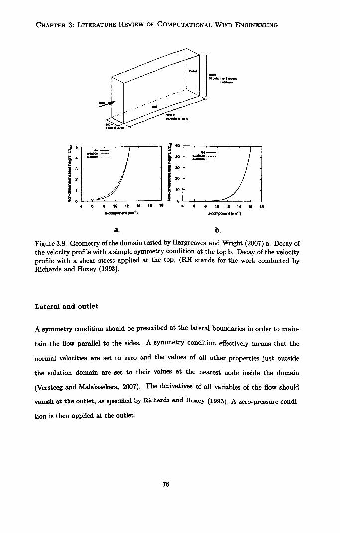
CHAPTER 3: LITERATURE REVIEW OF COMPUTATIONAL WIND ENGINEERING
soft 50Q 11119 q wd
1 OX . O.
-ýýýi
5
3
2
1
n
U -- M aý00ý rei0ý .......
46
40 80
20
10
6 10 12 14 +s to 4
(b "001l pmat (awl)
a. b
Figure 3.8: Geometry of the domain tested by Hargreaves and Wright (2007) a. Decay of the velocity profile with a simple symmetry condition at the top b. Decay of the velocity profile with a shear stress applied at the top, (RH stands for the work conducted by Richards and Hoxey (1993).
Lateral and outlet
A symmetry condition should be prescribed at the lateral boundaries in order to main-
tain the flow parallel to the sides. A symmetry condition effectively means that the
normal velocities are set to zero and the values of all other properties just outside
the solution domain are set to their values at the nearest node inside the domain
(Versteeg and Malalasekera, 2007). The derivatives of all variables of the flow should
vanish at the outlet, as specified by Richards and Hoxey (1993). A zero-pressure condi-
tion is then applied at the outlet.
76
66 10 12 14 10 10
u oompawf (I&)

CHAPTER 3: LITERATURE REVIEW OF COMPUTATIONAL WIND ENGINEERING
3.3.5 URANS
A key reason why RANS models are less suited to predicting wind loads than other engi-
neering problems is that the wind field is essentially unsteady. The incident wind is part
of a naturally turbulent ABL as shown in section 2.1.5; flow around a building structure
is dominated by local flow separation, reattachment and strong vortex structures; the
wake region is often dominated by vortices shed from the building as seen in section 2.2.
Consequently, even well defined flow regimes with symmetrical inlet conditions and a
symmetrical structure can generate unsteady loading patterns such as wake switching
(Prevezer et al., 2002). In these a steady BANS solution will not represent the true
loading situation.
For this reason, RANS is sometimes used in an unsteady simulations, called URANS.
URANS essentially introduces a temporal filter defined by the time step in the analysis
such that the longer period flow features are captured by the simulation. Although
this is often rightly criticised for lacking mathematical rigour (the RANS approach does
intrinsically time average the variables), it has been used to produce significantly bet-
ter estimates of wind pressure distributions that RANS models (Hanjalic and Kenjeres,
2008).
3.4 Large Eddy Simulation (LES)
3.4.1 Governing equations
LES is based on the idea that larger eddies are dependent on the geometry of the
disturbance and smaller eddies have a more universal and isotropic behaviour. In chapter
2, the energy cascade (how the energy is dissipated from the large scales to the smaller
scales), was presented. Since the larger scales interact with the main stream to extract
energy, they depend on the flow field, and therefore, on the geometry and the boundary
conditions.
In LES, the larger eddies, dependent on the geometry and the main flow, are resolved
77

CHAPTER 3: LITERATURE REVIEW OF COMPUTATIONAL WIND ENGINEERING
directly in a time-dependent simulation, while the smaller eddies are modelled. A spatial
filtering operation is used to distinguish the larger and the smaller eddies. This makes
LES a space averaging method as opposed to the time-averaging turbulence models
previously presented (RANS). The first step in LES consists of the filtering operation
which filters out the eddies smaller than the cut-off width and only retains the larger
eddies. The filtering of a variable 0 can be expressed as follows:
0(x, t) =J cb(x', t)G(x, x', /)dx' mnain
(3.4.1)
where O(x) is the filtered variable, the over-bar indicating spatial filtering, O(x) is the
unfiltered variable, G is the filtering function, and A is the cut-off width.
In commerical softwares, the cut-off width, 0, is chosen to be of the same order as the
grid size. Choosing a smaller cut-off width would be meaningless because any details
concerning eddies smaller than the grid size are lost as only a single value of each flow
variable is stored per grid cell (Versteeg and Malalasekera, 2007). The cut-off width is
often taken to be (OthyLz)1/3, where 0x, Ay, Oz are the grid sizes for the X, Y and
Z axes respectively.
After being filtered, the momentum equations are written as follows:
apui apu: ; ap -
aT, ý ät + ax,, 8x; axe + it div (grad (üti)) (3.4.2)
where the interaction between the resolved scales (larger eddies) and the unresolved
scales, also called Subgrid Scale eddies (SGS eddies), is contained within the subgrid-
scale stress rij, which can be written as follows, the prime indicating the unresolved
scales:
T{j = PUiU1 - offiuj
(Pu+ui - pu"uj) + (Pu-Wi + pu: uj) + (P; ) (3.4.3)
Lip + Cii + 17, j
78

CHAPTER 3: LITERATURE REVIEW OF COMPUTATIONAL WIND ENGINEERING
where
" Ltd are called the Leonard stresses and contain information on the resolved scales
exclusively.
" C11 are called the Cross-stresses and express the interaction between the resolved
and unresolved scales.
" Rij are also called the LES Reynolds stresses and are caused by convective moment
transfer between the SGS eddies. They are similar to the Reynolds stresses in the
RANS formulation and only involve unresolved eddies. As a result, they need to
be modelled. The different implementations of LES differ in the modelling of these
SGSs; a review of the most important approaches in OWE follows.
3.4.2 The key SGS models
The standard Smagorinsky-Lilly model, proposed by Smagorinsky (1963), was histori-
cally the first SGS model. The underlying idea of this SGS model is that the local SGS
stresses R; j are proportional to the local rate of strain of the resolved flow 5; j, which is
expressed as follows (Versteeg and Malalasekera, 2007):
Oqui R, j = -µscs axe + aui +3 Ridtj 3.4.4
where the SGS eddy viscosity is defined as:
µscs = PLa 131 (3.4.5)
with L. = min(Kd, CscsO), where r. is the von Karman constant, d is the distance to
the closest wall, and Cscs is a constant (151 = 2Sj; j).
Cscs is a constant in the standard Smagorinsky SGS model and has been optimized to
values between 0.1 to 0.25 according to Murakami (1997). Swaddiwudhipong and Khan
(2002) used the standard Smagorinsky SGS model for a 2D-simulation of the flow around
79
CHAPTER 3: LITERATURE REVIEW OF COMPUTATIONAL WIND ENGINEERING
a building surface, using CsGS = 0.1. They obtained a promising prediction of the flow,
including accurate prediction of the vortex shedding. Nevertheless, a lot of the key
features of the flow such as roof and side wall separation, and pressure distribution on
the building were lost because it was a 2D simulation.
In fact, because wind flow around a bluff-body involves very different regions of homo-
geneous conditions, choosing a universal value for the constant is problematic. This
implies the re-estimatation of the constant Cscs for each considered flow field, which
is not satisfactory. Furthermore, the standard SGS model has been proved to be overly
dissipative. This may be due to the fact that the model only accounts for the energy
cascade from large scales to smaller ones, and does not allow energy transfer from small
to larger scales, also called back scatter. That is why other SGS models have been pro-
posed, including a model where CSGS is a function of time and space. One of the most
prominent of these new models is the dynamic SGS model developed by Germano et al.
(1991).
The dynamic Smagorinsky-Lilly model for the subgrid scale stress allows the constant
CsGS to be dynamically modified based on the characteristics of the resolved eddies.
The dynamic procedure developed by Germano et al uses double filtering (Murakami,
1997):
Cscs 1 LijMtn 2 Mk2I (3.4.6)
where Lij are the Leonard stresses, previously defined in equation 3.4.3, and
M= n2I I ij - 21sIst; (3.4.7)
Porte-Agel et al. (2000) suggested a further optimization of the dynamic Smagorinsky-
Lilly model: The scale invariant assumption is relaxed in the near wall region. Near the
wall, the length scales become comparable to the distance to the wall. This new SGS
model was proven to perform better than the standard and the dynamic Smagorinsky-
Lilly models.
80

CHAPTER 3: LITERATURE REVIEW OF COMPUTATIONAL WIND ENGINEERING
Near wall modelling: In the LES formulation, it is assumed that the flow is going
to be resolved close to the wall; for this reason the first node must be placed very close
to the wall boundary, typically y+ < 5. However, it is possible to use wall functions if
the application does not allow a very fine mesh next to the wall. Breuer et al. (2007)
investigated wall models for LES in flow in plane channels; the underlying idea of the
wall models being the concept of artificial viscosity. This requires the definitions of the
distribution of the eddy viscosity in the outer layer and the thickness of the viscous
sublayer. Other works, including those of Tessicini et al. (2006,2007) have investigated
the efficiency of near wall models for LES. These are effectively zonal hybrid RANS-LES
models, and will be presented later.
Turbulent Inflow for LES: When using a k-e turbulence model, the variables input
at the inlet are either k and c or other variables directly related to k and e. Such sim-
plified and time-averaged inlet conditions cannot be used for LES. It is very important
to properly define a real turbulent wind inflow, namely a field of fluctuating velocities
reflecting the characteristics of the turbulent flow within the real ABL when running
LES. From the late nineties, when LES was first investigated in CWE, research groups
pointed out the need for techniques to generate turbulent inflows (Murakami, 1997,
1998). Since then, several methods for producing velocity fluctuations at the inlet of
the domain have arisen. A detailed review of the available methods have recently been
published by Tabor and Baba-Ahmadi (2010). Four of them are presented here.
The simplest one but certainly the most costly is the method using a precursor simula-
tion. The velocity field is stored at an appropriate downstream station of the precursor
simulation in an empty domain with roughness elements on the ground. This field is
then used as an inflow for the main simulation (Xie and Castro, 2008). This method
has been developed in 1993 by Mochida et al. (1993) and later by Thomas and Williams
(1999). The precursor simulation is as expensive as the main simulation. This makes
the whole process very demanding in terms of computer storage capacity, memory and
real time. However, the advantages of the method may justify such a cost. According
81

CHAPTER 3: LITERATURE REVIEW OF COMPUTATIONAL WIND ENGINEERING
to Thomas and Williams (1999) it is the only method able to reproduce the coherent
turbulent structures; it can also produce a wind spectrum that compared well with the
von Karman spectrum. However, the huge cost involved by the precursor method means
that it is not a viable option for practical industrial applications.
The second method of interest for the present work involves inverse Fourier transforms.
Inverse Fourier transforms are applied to prescribed spectra to produce artificial turbu-
lent inflows that respect given spatial and time correlations. This method was notably
described and assessed by Lee et al. (1992). However, Klein et al. (2003) later noticed
some disadvantages of the technique developed by Lee et al: it is both difficult to
program, and the use of Fourier transforms restricts the application to Cartesian and
equidistant meshes. Furthermore, it requires a 3D energy spectrum that is not easily
obtainable experimentally. The major disadvantage appears to be the randomness in
wave number space, that is, a realistic turbulence is only recovered after a long distance
(Klein et al., 2003; Xie and Castro, 2008). For these reasons, Klein et al. (2003) devel-
oped another technique achieving the same goal and based on the method presented by
Lee et al. (1992).
Klein et al proposed a technique that consists of filtering a set a random data using a
Gaussian filter. The filter is applied to three sets of 3D random data (2ND x NN x Nz
with N, Ny and Nz are the time length scale and the two spatial length scales) to
obtain a 2D turbulent inflow. Spatial and time correlation are ensured by a filter based
on a Gaussian autocorrelation function.
Later, Xie and Castro (2008) modified the method in order to make it more econom-
ical and this is the fourth method. Instead of using three sets of 3D random data,
their method only needs three sets of 2D random data (Ny X NN) and the time cor-
relation is guaranteed by a second filter. The second major change is the form of the
filter: Xie and Castro (2008) used a decaying exponential for defining the autocorrela,
tion function. This technique has been implemented in the present work with one or
two modifications, as described at length in Chapter 6.
82

CHAPTER 3: LITERATURE REVIEW OF COMPUTATIONAL WIND ENGINEERING
Application of LES to CWE: Murakami (1997,1998) reviewed a comprehensive
comparison of the static and the dynamic Smagorinsky models, along with other dynamic
SGS models. With regards to the computation, the author pointed out that one of the
main advantages of the static SGS model is its stability. Although the dynamic SGS
model does provide better numerical results, it is subject to stability problems due to the
large fluctuations of CSGS. As for the performance of the models: Where the static SGS
model did not predict any back scatter, the dynamic model significantly over predicts
it.
More generally, Murakami (1998) showed that the performance of the LES approach is
excellent compared with turbulence models:
" Unlike the k-e model and the Reynolds Stress Models, LES is able to predict the
impinging area and the separated area of the wind flow around a bluff-body with
excellent accuracy, even when the wind is not perpendicular to the structure.
" Unsteady phenomena, such as vortex shedding and other fluctuations are very well
reproduced by LES.
A recent study, conducted by Huang et al. (2007), compares the k-e model and LES
in the modelling of the flow around a tall steel building. Since they compared their
numerical results to outcomes of wind-tunnel studies, they modelled a 1: 250 scale model:
The domain featured a 73.55 cm high building. They used the dynamic kinetic energy
SGS model, which is one of the dynamic SGS models implemented within ANSYS-
Fluent. It is derived from the model developed by Kim and Menon (1997). It accounts
for the transport of the subgrid-scale turbulence kinetic energy, ksGS, that is defined in
the following equation:
kSGS =2 (uff - uk2) (3.4.8)
A transport equation for kscs derived from the standard k equation is solved:
2S a ökOt s+u Oxcs _ -r 18xß CE k0
f + äx (Qý Oä S) (3.4.9)
9 .7 .7
83

CHAPTER 3: LITERATURE REVIEW OF COMPUTATIONAL WIND ENGINEERING
The subgrid-scale stresses are defined as follows:
2 Tij -
2kSGSbii _ -2Ck kiGSOIsi. jI (3.4.10)
Figure 3.9 presents the computational domain used by Huang et al. (2007) and some of
their results in terms of mean velocity fields.
I
a. Computational domain
Velocity field,
top view
Yy
Velocity field,
side view
t
c. LES
Figure 3.9: Comparison of the standard k-f model and LES, wind flow around a tall building (after Huang et al. (2007)): (a) Computational domain, (b) and (c) Mean Velocity fields.
84
b. Standard k-epsilon model
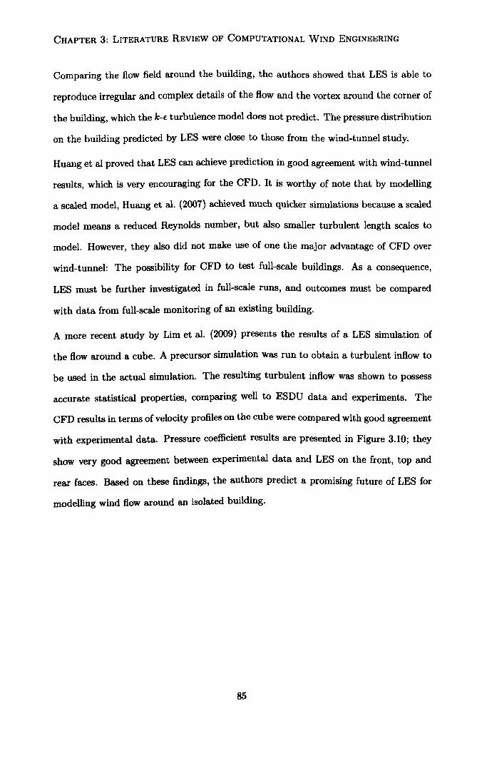
CHAPTER 3: LITERATURE REVIEW OF COMPUTATIONAL WIND ENGINEERING
Comparing the flow field around the building, the authors showed that LES is able to
reproduce irregular and complex details of the flow and the vortex around the corner of
the building, which the k-E turbulence model does not predict. The pressure distribution
on the building predicted by LES were close to those from the wind-tunnel study.
Huang et al proved that LES can achieve prediction in good agreement with wind-tunnel
results, which is very encouraging for the CFD. It is worthy of note that by modelling
a scaled model, Huang et al. (2007) achieved much quicker simulations because a scaled
model means a reduced Reynolds number, but also smaller turbulent length scales to
model. However, they also did not make use of one the major advantage of CFD over
wind-tunnel: The possibility for CFD to test full-scale buildings. As a consequence,
LES must be further investigated in full-scale runs, and outcomes must be compared
with data from full-scale monitoring of an existing building.
A more recent study by Lim et al. (2009) presents the results of a LES simulation of
the flow around a cube. A precursor simulation was run to obtain a turbulent inflow to
be used in the actual simulation. The resulting turbulent inflow was shown to possess
accurate statistical properties, comparing well to ESDU data and experiments. The
CFD results in terms of velocity profiles on the cube were compared with good agreement
with experimental data. Pressure coefficient results are presented in Figure 3.10; they
show very good agreement between experimental data and LES on the front, top and
rear faces. Based on these findings, the authors predict a promising future of LES for
modelling wind flow around an isolated building.
85

CHAPTER 3: LITERATURE REVIEW OF COMPUTATIONAL WIND ENGINEERING
ab I. J
0.5
Ü0
-0.5
g9
LES . tom. " as (M)
"r ný=r. R
"ý0 03 t 1.5 2 2.3 3
x'Ih
0
-0.4
u
-0.8
-1.2
-Ixs e 1v p. " RNS (2001
Top
Sick 6. ý Sick fQ
O 0.5 I 1.5 2 2.5 3
Y. /h
Figure 3.10: Results of pressure coefficient on a cube after Lim et al. (2009): comparison of LES, experimental data by Lim et al. and experimental data from Richards et al. (2001).
3.5 Hybrid RANS/LES models
Having presented the two ends of the spectrum of turbulence modelling, i. e. BANS and
LES, this section presents the alternatives to RANS and LES that fall into the category
of hybrid models. These models use URANS and LES in either a zonal or a seamless
approach. In a zonal approach, the zones in which URANS and LES are used are well
defined, generally the boundary layer is resolved by a URANS model, when the core
region is resolved by LES.
The most famous of the seamless hybrid models is the DES model (Detached Eddy
Simulation). This model effectively uses a RANS model in the near wall region in
an unsteady manner (also called URANS) and the Subgrid Scale Model (SGS) in the
outer LES region. The "seamless" switching between the approaches is done by chang-
ing the length scale. In the near wall region where RANS is used, the distance from
the wall is used to set the length scale, while in the LES region the grid size is used
(Hanjalic and Kenjere§, 2008).
A useful discussion is presented by Spalart (2001) when discussing meshing requirements
86

CHAPTER 3: LITERATURE REVIEW OF COMPUTATIONAL WIND ENGINEERING
for DES. With reference to Figure 3.11 (a corruption of Spalarts original figure), Spalart
defines a number of super regions: the Euler (ER), RANS and LES regions. The Euler
region covers most of the domain and is never entered by turbulence and can therefore
be covered by a fairly coarse, isotropic grid. Normal RANS gridding techniques are
applied in the RANS region, especially in the viscous or near-wall sub-region (VR).
Here the wall-normal dimension of the wall adjacent cell should be of an appropriate
size for the particular law of the wall being implemented in the DES model. Wall-
parallel dimensions are not such an issue. In the other BANS sub-region the outer
region (OR), similar gridding techniques to the ER can be implemented, with cell sizes
being too large for a switch to LES mode occurring. The switch does occur, however,
in the focus region (FR) where a target grid spacing should be created which allows
the LES turbulence model to be fully utilized. Cells should be isotropic in this region
to maintain computational efficiency, because often the filter length scale is the cube
root of the cell volume. Quite how large the FR should extend downstream is a matter
for experience although the major turbulent structures of the wake should be captured
in the FR. There then follows a departure region (DR) in which cells sizes smoothly
transition from those in the FR to those in the ER.
87

CHAPTER 3: LITERATURE REVIEW OF COMPUTATIONAL WIND ENGINEERING
ER
ER DR
J VR
rý OR i
ýr i
DR N. Figure 3.11: Flow regions in DES (modified version of a sketch by Spalart (2001)).
Originally, the RANS model used for DES was the one-equation model, the Spalart-
Almaras model (details in Nikitin et al. (2000)), which was used in both regions. Later
this was improved by using more advanced RANS based model, such as the SST k-w (see
section 3.3.2). In this formulation of the DES model, the dissipation term in Equation
(3.3.9), which was equal to, 3*kw becomes ß*kWFDES where
FDES = max (Lt/(CDES A), 1)
CDES is a calibration constant, equal to 0.61,0 is the maximum local cell size, and
Lt =W the turbulent length scale of the RANS model. This expresses that the
DES length scale LDES is equal to the RANS length scale in the near wall region
(LDES = Lt), where Lt < LDES. In the LES region, where the turbulent length scale
is larger than the DES length scale, LDES = CDESA. Effectively, the SST k-w model
is used in the boundary layer, while the LES formulation is applied in the separated
regions. Hanjalic and Kenjere§ (2008) noted that there is some degree of arbitrariness
88

CHAPTER 3: LITERATURE REVIEW OF COMPUTATIONAL WIND ENGINEERING
in the DES model: The switching between two zones is determined by the size of the
grid cells, even though the constant CDES can be changed to tune the switching to the
desired level. Despite this, DES is still a good alternative to LES, as it saves significant
computing resources and time, while solving a lot more turbulent length scales than a
simple RANS model.
Davidson and Peng (2003) have used this hybrid RANS-LES based on the k-w turbu-
lence model for predicting flow in a plane channel, Figure 3.12. They found that the
mean flow was well predicted even with a coarse mesh. Some inconsistencies at the
RANS-LES interface were also found. The major problem they noted was that the
flow provided by the RANS region to the LES region did not have the proper spectral
properties, or in other words LES was given poor information by RANS. This loss of
information in the small scales (high frequency) was also observed by Tessicini et al.
(2006). In order to solve this issue, Davidson and Peng suggested adding turbulent fluc-
tuations to the mean quantities transferred from the BANS region to the LES region.
They presented the results of such an approach in Davidson and Billson (2006). The
authors actually implemented isotropic turbulent fluctuations, and then non-isotropic
fluctuations. The isotropic fluctuations were found to be sufficient to greatly improve
the flow prediction, as much as the non-isotropic fluctuations. However, it must be
noted that the isotropic fluctuations are taken from a previous DNS simulation, which
does not make this approach practical for a wide range of applications.
near-wall BANS region
----------------------------------------------------
core LES region V
- ---------- near-wall RANS region + Yrnf
Figure 3.12: The near wall BANS region and the core LES region for modelling flow in a plane channel flow (after Davidson and Peng (2003)).
89

CHAPTER 3: LITERATURE REVIEW OF COMPUTATIONAL WIND ENGINEERING
Tessicini et al. (2006,2007) have presented results of a zonal hybrid RANS-LES model
for high Reynolds numbers flow. The one equation RANS model they used for the
near wall region represented a significant improvement from an analytically prescribed
log-law wall function (Figure 3.13). The acceptable load on computing resources makes
this method practical for industrial applications. It was also observed that the hybrid
RANS-LES model applied to a relatively coarse mesh performed better than simple
LES, which is consistent with the mesh refinement requirements for LES.
LES --BANS &"a LES lal (nýAar
a -0110 -""
----------- -- " --------------- -------
RAAti pO yroc"ad
-----ý-----p----i----- O r+latafire
(b) OS"1
-----------------
IFS
pf-r" r.,, v-f-
Figure 3.13: Illustration of the hybrid RANS-LES model in the near wall region (a)
and the analytically defined logarithmic law of the wall (b) after Tessicini et al. (2006): hybrid RANS-LES showed better performance than the log-law at the wall.
Such hybrid models with a one-equation RANS model for the near wall region were also
applied with success by Breuer et al. (2008); Temmerman et al. (2003). Temmerman et al.
(2005) compared the use of one equation and two-equation RANS models for the near
wall region, in association with LES. They concluded that the hybrid RANS-LES models
showed potential. They noted that the models performed better when the RANS-LES
interface was located further away from the wall, which indicates that the RANS model
is more suited to predicting the near wall flow than LES. This can be explained by the
fact that the mesh they used was probably too coarse for a pure LES simulation for
which the mesh needs to be greatly refined near the wall (y+ < 5). For any coarser
mesh, RANS can be expected to perform better than LES in the near wall region.
90

CHAPTER 3: LITERATURE REVIEW OF COMPUTATIONAL WIND ENGINEERING
The same observation was made by Senocak et al. (2007): The hybrid RANS-LES model
performed better in the prediction of the logarithmic profile in the near wall region than
LES with dynamic Smagorinsky-Lilly SGS model. Senocak et al. suggested that this
may be due to the fact that the BANS model, used in the hybrid model, takes the
distance to the wall as length scale, and this can be shown analytically to give a log-law
profile.
Hybrid RANS-LES models are very promising as they combine the accuracy of LES in
the fully separated regions, and the robustness and flexibility of RANS based models in
the boundary layers, saving significant computing power compared to LES by reducing
the number of cells needed in the near wall region.
The good performance at acceptable computing cost of hybrid RANS-LES models are
the reason why one of these models, the DES model, is used for the present work in
some cases, and in particular for testing the fluid-structure interaction tool, as presented
in Chapter 5.
3.6 Summary and conclusions
This chapter presented how CFD can be applied to wind engineering problems with
a review of the models used in CWE, including the RANS turbulence models, as well
as LES and the hybrid RANS/LES models. It was shown that RANS models can be
used to obtained good approximations of the mean properties of the flow, despite some
major limitations, notably in the prediction of recirculation regions. Hybrid RANS/LES
models were shown to combine the advantages of RANS (relatively low computing re-
sources needed) with those of LES (accuracy in the key regions, such as the wake). As
a consequence, the hybrid RANS/LES DES model is used in the present work when
possible.
The size of the computational domain was not discussed in this chapter as it is the
object of the next chapter to investigate the current recommendations of domain sizes
for modelling flow around tall buildings, and to challenge them.
91

Chapter 4
Size of the computational domain
4.1 Introduction
As the objective of this work is to study the flow around tall buildings, it was necessary
to build numerous meshes in order to test the tools that were developed as part of
this work. Religiously following the recommendations published by Franke et al. (2007)
and Ranke et al. (2004) generates particularly large domains. Such large domains are
expensive in computational terms. Thus, it was decided to investigate smaller domain
sizes and study the impact of this domain size reduction on the key flow variables.
This way, it could be determined whether smaller domain sizes could be used while
maintaining reasonable predictions of the flow.
4.2 Background
A key part of the modelling is the choice of the domain size and the positioning of the sin-
gle tall building within that domain. Recent CFD studies have used Franke et al. (2004)
as a starting point in determining the domain size. A later document (Franke et al.,
2007) updates these recommendations but adds very little to the previous document in
terms of the discussion about domain size. It does refer to a Verein Deutscher Ingenieure
(VDI) publication which suggests that the blockage ratio should be less than 3%, based
92

CHAPTER 4: SIZE OF THE COMPUTATIONAL DOMAIN
largely on wind tunnel modelling experience.
There is considerable evidence of the recommendations published by Franke et al. (2007)
and Franke et al. (2004) being adhered to by workers when modelling low-rise buildings.
For example, Figure 4.1 is taken from Franke (2007) and shows the domain used by
Wright and Easom (2003) to model the Silsoe cube, which is described in Hoxey et al.
(2002). For such low-rise buildings, where H-B-L (with B and L being the
cross- and alongwind building dimensions respectively), these requirements produce
domains that are both acceptable in physical and computational terms. By "acceptable
in.. . computational terms", it is meant that the domain boundaries are not so distant
from the building that the number of computational cells required to fill the domain to
ensure a reasonable level of accuracy becomes too large.
Figure 4.1: Computational domain taken from Franke (2007)
However, when the aspect ratio of the building changes and H»L, B, as is the case
for tall buildings, the domain size chosen by workers is open to more interpretation.
There is a small, but increasing, body of work using CFD to model: 1) wind loads on;
2) pedestrian level comfort close to; and 3) rainfall around tall buildings. An analysis
of this work is presented in Table 4.1, which includes the guidelines for comparison.
Wherever possible, the length of the domain, 1, is shown as a sum of three components:
lu, L and Id, the upstream fetch, the building length in the alongwind direction and the
downwind fetch, respectively. Similarly, the width of the domain, b, is broken into three
components: bd, B and b9 (most domains are symmetrical and so bd = b9, typically).
The height of the domain, h, has only two components: H and h8, the latter being the
93
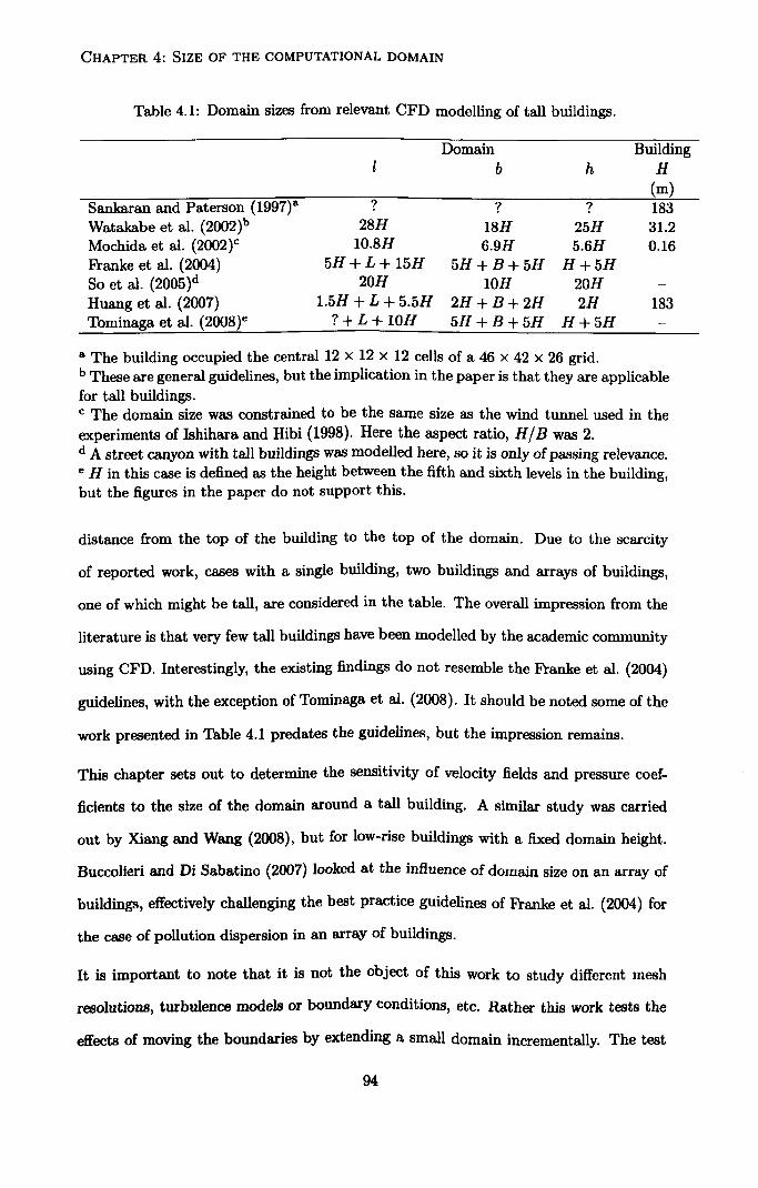
CHAPTER 4: SIZE OF THE COMPUTATIONAL DOMAIN
Table 4.1: Domain sizes from relevant CFD modelling of tall buildings.
Domain Building b h H
(m)
Sankaran and Paterson (1997)a ? ? ? 183 Watakabe et al. (2002)b 28H 18H 25H 31.2 Mochida et al. (2002) 10.8H 6.9H 5.6H 0.16 Franke et al. (2004) 5H +L+ 15H 5H+B+5H H+5H So et al. (2005)d 20H 10H 20H - Huang et al. (2007) 1.5H +L+5.5H 2H +B+ 2H 2H 183 Tominaga et al. (2008)e ? +L+1OH 5H+B+5H H+5H -
a The building occupied the central 12 x 12 x 12 cells of a 46 x 42 x 26 grid. b These are general guidelines, but the implication in the paper is that they are applicable for tall buildings. C The domain size was constrained to be the same size as the wind tunnel used in the experiments of Ishihara and Hibi (1998). Here the aspect ratio, H/B was 2. dA street canyon with tall buildings was modelled here, so it is only of passing relevance. eH in this case is defined as the height between the fifth and sixth levels in the building, but the figures in the paper do not support this.
distance from the top of the building to the top of the domain. Due to the scarcity
of reported work, cases with a single building, two buildings and arrays of buildings,
one of which might be tall, are considered in the table. The overall impression from the
literature is that very few tall buildings have been modelled by the academic community
using CFD. Interestingly, the existing findings do not resemble the Franke et al. (2004)
guidelines, with the exception of Tominaga et al. (2008). It should be noted some of the
work presented in Table 4.1 predates the guidelines, but the impression remains.
This chapter sets out to determine the sensitivity of velocity fields and pressure coef-
ficients to the size of the domain around a tall building. A similar study was carried
out by Xiang and Wang (2008), but for low-rise buildings with a fixed domain height.
Buccolieri and Di Sabatino (2007) looked at the influence of domain size on an array of
buildings, effectively challenging the best practice guidelines of Franke et al. (2004) for
the case of pollution dispersion in an array of buildings.
It is important to note that it is not the object of this work to study different mesh
resolutions, turbulence models or boundary conditions, etc. Rather this work tests the
effects of moving the boundaries by extending a small domain incrementally. The test
94

CHAPTER 4: SIZE OF THE COMPUTATIONAL DOMAIN
case described in Section 4.3 is for a 1: 200 scale 180 m building, with a large aspect
ratio. This work was motivated by the fact that the recommendations of Franke et al.
(2004) produced very large domains for high rise buildings. This is largely due to H
being used as the characteristic length scale upon which the dimensions of the domain
are based. The resulting large domain implies a very large number of cells, which is
expensive in terms of computing power and time. The underlying idea was, therefore,
to generate new, practical recommendations for the size of the domain for tall buildings.
4.3 Case study
The computational work described in this paper was carried out using ANSYS Fluent,
version 12.
4.3.1 Domains and meshes
The building chosen for this work is a 1: 200 scale rectangular prism with full-scale
dimensions of H= 180 m, L= 10 m and B= 20 m (0.9 m by 0.05 m by 0.1 m at scale).
This prism is placed in a rectangular domain, the dimensions of which are varied. Four
domains were created for the study:
Small whose dimensions respected a 3% blockage ratio (ratio of the front area of the
building over the inlet area).
Medium which is an extension of the small domain, but only in the yz-plane, to create
a 1.5% blockage ratio.
Medium 2 which has the same blockage ratio as the medium domain, but is extended
upwind and downstream.
Large which was built according to the recommendations of Franke et al. (2007).
The dimensions of these four domains are summarized in Table 4.2 and shown schemat-
ically in Figure 4.2.
95
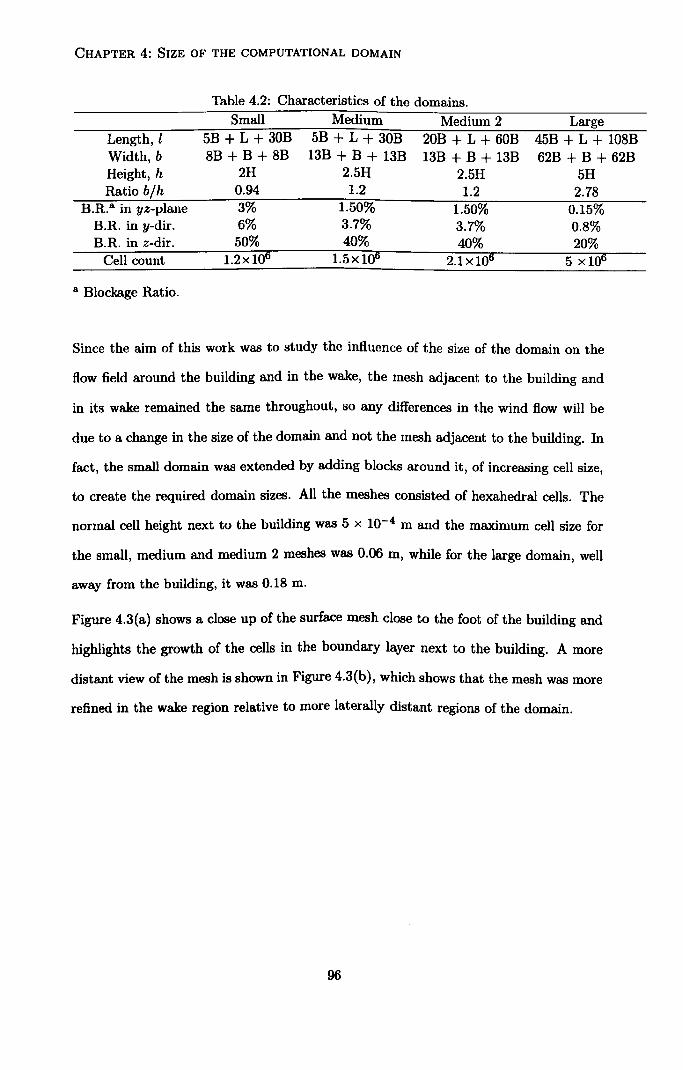
CHAPTER 4: SIZE OF THE COMPUTATIONAL DOMAIN
Table 4.2: Characteristics of the domains. Small Medium Medium 2 Large
Length, l 5B+L+30B 5B+L+30B 20B +L+ 60B 45B +L+ 108B Width, b 8B +B+ 8B 13B +B+ 13B 13B +B+ 13B 62B +B+ 62B Height, h 2H 2.5H 2.5H 5H Ratio b/h 0.94 1.2 1.2 2.78
B. R. a in yz-plane 3% 1.50% 1.50% 0.15% B. R. in y-dir. 6% 3.7% 3.7% 0.8% B. R. in z-dir. 50% 40% 40% 20%
Cell count 1.2x10 1.5x10 106 5 x10
a Blockage Ratio
Since the aim of this work was to study the influence of the size of the domain on the
flow field around the building and in the wake, the mesh adjacent to the building and
in its wake remained the same throughout, so any differences in the wind flow will be
due to a change in the size of the domain and not the mesh adjacent to the building. In
fact, the small domain was extended by adding blocks around it, of increasing cell size,
to create the required domain sizes. All the meshes consisted of hexahedral cells. The
normal cell height next to the building was 5x 10⁻⁴ m and the maximum cell size for
the small, medium and medium 2 meshes was 0.06 m, while for the large domain, well
away from the building, it was 0.18 m.
Figure 4.3(a) shows a close up of the surface mesh close to the foot of the building and
highlights the growth of the cells in the boundary layer next to the building. A more
distant view of the mesh is shown in Figure 4.3(b), which shows that the mesh was more
refined in the wake region relative to more laterally distant regions of the domain.
96

CHAPTER 4: SIZE OF THE COMPUTATIONAL DOMAIN
SH
_ý x
`- rý
----------- --------------------------------------------------------------------------
4 45B
Iii 2SH
----- --- -//
I
smri
Median 2
Lur
Figure 4.2: Dimensions of the four domains.
-----------------------
97
a9 'I'
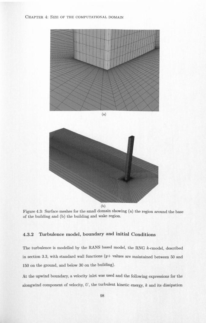
CHAPTER 4: SIZE OF THE COMPUTATIONAL DOMAIN
(a)
(b) Figure 4.3: Surface meshes for the small domain showing (a) the region around the base
of the building and (b) the building and wake region.
4.3.2 Turbulence model, boundary and initial Conditions
The turbulence is modelled by the RANS based model, the RNG k-e model, described
in section 3.3, with standard wall functions (y+ values are maintained between 50 and
150 on the ground, and below 30 on the building).
At the upwind boundary, a velocity inlet was used and the following expressions for the
alongwind component of velocity, U, the turbulent kinetic energy, k and its dissipation
98

CHAPTER 4: SIZE OF THE COMPUTATIONAL DOMAIN
rate, e from Richards and Hoxey (1993) were used:
ý z+zo U(z) = u* In
z), (4.3.1)
ZO U2
k(z) =* (4.3.2)
3
e (z) =ý (4.3.3) rc(z + zo),
where is is von Karman's constant and zo is the surface roughness length. Equation 4.3.1
is a standard representation of the velocity profile in the ABL. In the present work,
zo = 0.001 m and u, t = 0.11 ms-1. No attempt, however, was made to modify the
turbulent Schmidt number, o,,, as suggested by Richards and Hoxey (1993), because it
is not clear how this could be incorporated in the RNG framework.
At the downwind boundary, a pressure outlet was used, with the relative pressure speci-
fied at 0 Pa and backflow conditions for k and e set to those of the inlet. In all domains,
however, backflow was not observed because the downwind boundary was sufficiently far
from the building. The low- and high-y boundaries were set as symmetry conditions,
as was the high-z boundary. A shear stress was not applied at the top boundary, as
suggested by Richards and Hoxey (1993) because of the variable height of the domain
between cases.
Equations 4.3.1 to 4.3.3 were used to specify the field variables throughout the domain
as initial conditions at the start of the steady--state simulation.
4.3.3 Solver settings
As mentioned in Section 4.3.2, the solutions were steady-state. Second-order differenc-
ing was used for the momentum and turbulence equations and the convergence criteria
were set to 10-4. However, this was not the only test for convergence - the drag, lift
and side forces as well as the moments acting on the building were monitored during the
simulation and only when they achieved constant values were the simulations deemed
to have converged.
99

CHAPTER 4: SIZE OF THE COMPUTATIONAL DOMAIN
4.4 Results and discussion
Figure 4.4 shows contour plots of the velocity magnitude at the mid-height of the
building for the four domains. At first glance, they all present a very similar wake
pattern, showing, as might be expected with a steady RANS simulation, a symmetrical
wake. The free stream velocity appears to be higher for the small domain than for
the three other domains. This is due to the proximity of the lateral boundaries to the
building and is clearly a blockage issue. For the three other domains, the more distant
lateral boundaries serve to reduce this effect.
Similarly, Figure 4.5 shows contour plots of the velocity magnitude on a vertical plane,
located at the centre of the domain. As in Figure 4.4, the general pattern is very similar
for the four domains. There is a low velocity region located at about H/2 downstream
and at mid-height of the building for the four domains, which corresponds to the centre
of the major recirculation behind the building. Again, for the small domain the flow
does not fully recover to the freestream near the top boundary as it does for the two
medium and the large domains.
The velocity profiles upstream and downstream the building, illustrated in Figure 4.6,
exhibit very good agreement for the four domains. A slight decay in the velocity can
be observed for the large domain, which can be attributed to the much longer fetch
upstream the building. The velocity profiles downstream the building in the wake do
not highlight any significant differences between the four domains. This tends to indicate
that the four domains have their lateral boundaries located far enough from the building
so as not to significantly influence the flow in the wake. In order to investigate this
further, a "width of the wake", Bw, was computed on a horizontal plane at the mid-
height of the building for the four cases. It is presented in non-dimensionalised form
in Figure 4.7(a). The wake was defined to be the region in which the velocity is lower
than 0.9UH/2 i where UH/2 is free stream velocity at a height H/2 as determined from
Equation 4.3.1. Here, the small and medium domains have similarly sized wake widths,
whereas the medium 2 and large domains form another group. It is not clear how the
100

CHAPTER 4: SIZE OF THE COMPUTATIONAL DOMAIN
(a) (b)
SS
(c) (d)
Figure 4.4: Contours of velocity magnitude on a horizontal plane at z= H/2 for the (a)
small, (b) medium, (c) medium 2 and (d) large domains.
101

CHAPTER 4: SIZE OF THE COMPUTATIONAL DOMAIN
0 OOe"00 3 15. C1 6 30. C1 945.01 1 26-00 1 57e. 00 1 99e-00 2 10e. 00
(a)
ý-+
lý) (d) Figure 4.5: Contours of velocity magnitude on a vertical plane at y=0 for the (a) small, (b) medium, (c) medium 2 and (d) large domains.
pl
(b)
102

CHAPTER 4: SIZE OF THE COMPUTATIONAL DOMAIN
extra upwind fetch of the medium 2 domain (over the medium domain) should lead to
a much wider wake, when it might be expected that the lateral boundaries would play
more of a role. A more convincing argument is that the change in the velocity profile
between the two medium domains is responsible for the difference.
Figure 4.6: Comparison of velocity profiles on a vertical rake on y=0 at 5L upstream, 1OL downstream and 25L downstream of the building for the small, medium and large domains.
In addition, Figure 4.7(b) shows the behaviour of the so-called "wake depression", which
is defined here as the (UH/2 - Umin)/UH/2, where Umin is the minimum value of velocity
on a horizontal line at right angles to the wind direction and UH/2 is the wind speed
at half the building height (shown as Uo in the figure). So, a value of 1 for the wake
depression equates to zero velocity magnitude, as can be seen for all domains at a
distance x- 1OL = H/2 downstream of the building, which corresponds well with
the centre of the low velocity region seen in Figure 4.5. From this point, the velocity
magnitude recovers back towards UH/2. Far from the building, the trend that the
smaller domains have a greater depression is clear. This can be explained by the higher
blockage ratios in the smaller domains creating higher wind speeds around the building
and a more intense wake, the strength of which is related to the free stream velocity.
Evidence for this can be found in Eskridge and Hunt (1979), who look, theoretically, at
103

CHAPTER 4: SIZE OF THE COMPUTATIONAL DOMAIN
the development of a wake behind a moving vehicle.
A, dtl. nce from building (a)
e
S
5 1D 15 40 25 30 35 An ýc c. w4 daw" nom buffaig --
(b)
Figure 4.7: Comparison of (a) wake widths and (b) wake depressions for all domains.
104

CHAPTER 4: SIZE OF THE COMPUTATIONAL DOMAIN
a I
1
wp ...... .... ööavvovvý }
°vvvö oööv°
0
(a)
,.
s ýa
1' I
vvv Vý vv
v v . swt
ý
i
4.0 iý
4. vv
,. "y
.. w V o
.g
Y
.
eý
6`
d a
I a
(b)
(c) (d) Figure 4.8: Pressure coefficients, CPI on lines (a), (b) and (c), shown in plot (d).
Finally, and perhaps most significantly, pressure coefficients along several lines over the
building are presented in Figure 4.8(a) to (c). The locations of the lines are shown in
Figure 4.8(d) and on the plots, the non-dimensionalised distance along each line s/L is
used, where s is the distance from the start of the line. The pressure coefficient, Cp, is
defined as: P- Pref Cp= 2pUH
where UH is the wind speed at height H and pref is defined as the average pressure on
the outlet, in this case 0 Pa relative. It should be noted that the pressure coefficients are
deliberately not corrected by the free stream velocity in the domain, as this would be the
equivalent of applying a blockage ratio correction to the results. The lines (a) and (b)
shown in Figure 4.8(d) have been deliberately chosen to pass over the roof because this
105

CHAPTER 4: SIZE OF THE COMPUTATIONAL DOMAIN
is where much of the interest for low-rise buildings lies. Pressures on the roof are less of
an issue when analysing the dynamic response of a tall building, which is often driven
by pressure differences between the long, vertical walls of the building. Nonetheless, the
pressures acting on the roof of a high-rise building are still important in terms of debris
release during storms, for example.
The pressure coefficients appear to be more sensitive to the blockage ratio than the
velocity is. The pressure coefficients on line (a) display higher suction on the roof for
the smaller domains'. The difference between the two medium domains is negligible,
while the difference between the small and large domains approaches 40% on the roof.
As mentioned, on the roof, the two medium domains exhibit similar results, which can be
explained by the fact that the domain height (2H and 2.5H) is roughly the same in each
case. The large domain which has a top boundary located much higher (5H) shows lower
suction on the roof. This would indicate that 2.5H is indeed too small to accurately
resolve the pressure distribution on the roof, and that the 5H recommendation should
be followed.
Figure 4.8(b) paints a less dramatic picture, but this is due to the much greater range
of pressure coefficients seen on this line. At the mid-point of the roof, there is still the
large discrepancy in Cp between the small and large domains. However, on the front face
(0 < s/L < 1), the differences between the domains are, in percentage terms, less than
10%. The fact that the medium 2 and large domains agree more closely on the front
face in both plots (b) and (c), indicates that the pressures here are very sensitive to any
decay in the velocity profile for these slightly longer upwind fetches. However, the large
domain still has an upwind fetch twice that of the medium 2 domain, but this would
indicate that a shorter upwind fetch, here 20B, than that suggested by Franke et al.
(2004) is acceptable.
The pressure coefficients on the leeward face, in Figure 4.8(b) and (c) indicate that a
much larger downstream distance is unlikely to greatly influence the results. Therefore,
'The traverse (a) in Figure 4.8 goes from one side of the building to the other and has been left like this to demonstrate the symmetry of the pressure field.
106

CHAPTER 4: SIZE OF THE COMPUTATIONAL DOMAIN
a downstream distance of 30B seems to be enough to let the wake develop, without any
danger of the outlet boundary unduly influencing the results. The pressure coefficients
on the side face at mid-height of the building, 1< s/L < 2, indicate that the medium 2
and large domains produce results that are within 5% of each other, except in the critical
zone just downstream of the leading edge of the building.
4.5 Summary and new recommendations
The aim of this chapter was to provide some guidance as to what size of domain should
be used when modelling tall buildings using CFD. It is intended as an extension of the
admirable work of Franke et al. (2004) for low-rise buildings. It should be re-iterated
that this was a parametric study with only one parameter; the domain size. Although
the use of a steady R. ANS model in the context of wind engineering is flawed, that
this modelling approach does give a satisfactory representation of the blockage effects
supports its use here. With this in mind, from the discussion of the results in §4.4, the
following conclusions can be drawn:
" Pressure coefficients and velocity fields are sensitive to domain size, which confirms
observations from wind tunnel blockage ratio studies for many years
e Assuming that the large domain provides the benchmarking data, under the
premise that infinitely distant boundaries would be desirable, the small domain is
simply too small to provide acceptable results: the relative errors of the small do-
main compared to the large domain are significantly larger than 5-10% as shown in
Section 4.4 (the disagreement reaches 40% of the pressure coefficient on the roof).
This suggests that the 3% blockage ratio suggested by VDI is not acceptable.
. The smaller differences between the medium 2 and large domains suggest that the
following (tentative) guidelines for domain size with a tall building are appropriate:
- Upwind fetch, 1: 20B or 2H, whichever is the greater.
- Downwind fetch, Id: 30B or 3H, whichever is the greater.
107

CHAPTER 4: SIZE OF THE COMPUTATIONAL DOMAIN
- Top clearance, h8: 4H.
- Side clearances, bd and b9: > 13B, and such as the ratio b/h >1
which can be compared with the corresponding recommendations of Franke et al.
(2004), which are: 5H, 15H, 5H and 5H respectively
Therefore, for the particular case presented here, this represents a reduction in the
volume of the domain of approximately 90%. This constitutes a significant reduction
in the number of cells required, even if the mesh can be coarsened away from the
building/wake region.
4.6 Application of the new recommendations
Following these recommendations, a new mesh was created. The characteristics of the
new mesh called the Final Recommendations (FR) domain are presented in Table 4.3.
The new domain represents a saving of 88% in terms of volume, and a saving of 30% in
number of cells, while still respecting a blockage ratio of less than 1% in the y-z plane.
For the FR domain, the mesh was slightly refined in the outer region since a lot of the
volume could be saved compared to the large domain. It shows that by applying the
new recommendations, the mesh can be refined while still reducing the number of cells
significantly.
Table 4.3: Characteristics of the mesh following the Final Recommendations (FR Final Recommendations (FR) COST recommendations
Length, I 20B +L+ 30B 45B +L+ 108B Width, b 26B +B+ 26B 62B +B+ 62B Height, h 5H 6H Ratio b/h 1.2 2.78
B. R. ° in yz-plane 0.75% 0.15% B. R. in y-dir. 2% 0.8% B. R. in z-dir. 20% 16%
Cell count 3.5 x 10 5x 10
I Blockage ratio.
Figures 4.9 and 4.10 show the velocity magnitude for the FR and large domains. Similar
108

CHAPTER 4: SIZE OF THE COMPUTATIONAL DOMAIN
I DO. " 3 i5. C1 8 JO. C1 945. Cl 178e. 00 1 57e. 00 1 99e X00 2 10e. 00
m
1º
(8) (b)
Figure 4.9: Contours of velocity magnitude on a horizontal plane at z= H/2 for the (a) FR ("optimum" in the legend), (b) large domains.
flow fields are obtained with both domains. It can be seen that the wake does not show
dramatic differences in Figure 4.9 even though the large domain is more than twice as
wide as the FR domain. Figure 4.10 shows that the flow fields in the x-z plane are
again very similar for the large and FR domains. The point where the velocity reaches
a minimum in the wake is located at approximatly H/2 downstream the building for
both domains. The similarity is confirmed by the velocity profiles plotted upstream and
downstream the building, presented in Figure 4.11.
Figure 4.12 (a) presents the width of the wake for all the domains (as defined previously).
The FR domain has a similar wake of the width to the one exhibited by the large domain.
The fact that the FR domain is wider than the medium and medium 2 domains could
explain the slightly larger width of the wake, closer to the large domain. As for the
velocity in the wake, shown in Figure 4.12 (b), the maximum depression occurs at the
same location downstream the building for the FR and medium 2 domains, which may
be explained by their similar downwind fetch.
The last results presented are the ones regarding the pressure distribution on the build-
ing, Figure 4.13. The largest differences are exhibited in (a) with a relative error of
11% but it must be noted that a smaller range of pressure is shown in this distribution
109

CHAPTER 4: SIZE OF THE COMPUTATIONAL DOMAIN
LI (a) (b)
Figure 4.10: Contours of velocity magnitude on a vertical plane at y=0 for the (a) FR ("optimum" in the legend), (b) large domains.
c
t
c
c
.. _ý _ .' Kýe.. 'ý a45e-Ot t : 6e oC 5/e "uU 1 , aeon 210, "00
L 1
wWl domain
6 medium domain -- medium 2
- large domain 6 - opänu domain
.4
2
i
Unll Ulu.
I
_ _ ___ -10 0 10 20 30 40 50 60
Figure 4.11: Comparison of velocity profiles on a vertical rake on y=0 at 5L upstream, 10L downstream and 25L downstream of the building for the small, medium, large and FR ("optimum" in the legend) domains.
110

CHAPTER 4: SIZE OF THE COMPUTATIONAL DOMAIN
co
I
18
- small
medium -- medium 2
14 arye oplimum
12
10
5 10 15 N. , n+ 35 40 45 50 x/L, diWnn from building
(a)
-. mat medun
- medWm i - feige
1 ---np°mum
ae
0.4
02
0 °5 10 1s 20 25 30 35 40 45
XIL. am" ýDM. V
(b)
Figure 4.12: Comparison of (a) wake widths and (b) wake depressions for all domains including the FR domain ("optimum" in the legend).
111

CHAPTER 4: SIZE OF THE COMPUTATIONAL DOMAIN
. ..... ......
(a)
a
l{o t 1
.:
Y
iiiiiiiii
i. ,: i
4 ýt
4
. ßs
10
(b)
-;....... ý w (c) (d)
Figure 4.13: Pressure coefficients, Cp, on lines (a), (b) and (c), shown in plot (d) for all domains including the FR domain ("optimum" in the legend).
than in (b) and (c). The pressure distribution on the front face in the FR domain is
similar to the large domain. On the side faces of the building, the pressure distribution
in the FR domain is closer to the one in the medium 2 domain, although this is not
clear in (c) where the results for the FR and the large domain appear to be very close.
On the leeward face, as it was observed for the four domains in Figure 4.8, the results
for the five domains are in very good agreement, which would tend to indicate that the
downwind fetch for the FR is long enough.
Generally, the FR domain shows results that are very close to the one shown by the
large domain, while saving a significant amount of computing resources allowing for a
smaller domain to be used.
112

CHAPTER 4: SIZE OF THE COMPUTATIONAL DOMAIN
4.7 Conclusions
In this chapter, it was attempted to define new recommendations for the size of the
computational domain for tall buildings. This study was motivated by the fact that the
existing guidelines appear to have been defined for low to mid-rise buildings, leading
to extremely large computational domains for high aspect ratio structures (height over
width), such as slender and tall buildings. The study focused on the size of the domain
solely, and not on other aspects such as mesh refinement, and turbulence models. The
comparison of the results for domains of increasing sizes lead to the definition of new
recommendations for this particular geometry that could be used for modelling the wind
flow around tall buildings while maintaining an acceptable level of accuracy. These
new recommendations were applied; the flow field and the pressure distribution on the
building in this new domain were compared with the other domains. It was found
that the new recommendations gave results that compared well with results obtained
when following Franke et al. (2004). As a consequence, in the next chapters, the new
recommendations are followed, sometimes with slight variations, in order to use the
computing resources with better efficiency.
113

Chapter 5
Fluid-structure interactions
5.1 Introduction
This chapter aims to introduce a method for fluid-structure interactions (FSI), in order
to address the first intermediate objective: to develop and evaluate a numerical tool in
order to account for the dynamic response of the building to wind loading, and to assess
the coupling of the building motion and the wind flow.
After a short review of the methods for FSI and their applications to wind engineering,
the method developed for this work is described in detail. Then, the results of the
application of the method to a 180 m building are presented.
5.2 Review of the method for modelling fluid-structure
interactions
5.2.1 Introduction
Three elements are usually distinguished when solving fluid-structure interactions: the
fluid, the structure and the mesh. The stresses and displacements of the structure are
calculated from the fluid computation. The fluid mesh is then moved accordingly to the
structure displacements, and the effects of such displacements are accounted for by the
114

CHAPTER 5: FLUID-STRUCTURE INTERACTIONS
fluid solver.
The governing equations are composed of the well-known Navier-Stokes equations for
the fluid and the following equations for the structure:
Mil + Cü + Ku = F8(t) (5.2.1)
where u is here the displacement vector of the structure, M the mass matrix per unit
span, C the damping matrix, K the stiffness matrix, and Fe (t) the time-dependent
force due to wind loading.
5.2.2 Fluid-mesh coupling
The third element to account for in FSI is the movement of the mesh. One sensitive
part is how the motion of the fluid is handled within the moving mesh. The Arbitrary
Lagrangian Eulerian (ALE) method is used in most cases to deal with that issue.
The idea for ALE is to combine Lagrangian and Eulerian approaches. The Lagrangian
method is usually used in solid mechanics and also in fluid mechanics when one wants to
follow individual particles: in such view, the grid is allowed to deform with the solid or
the particle. In particular, this means that the displacement of each particle is calculated
and the nodes of the mesh correspond to the particles, which limits the extend to which
the particle can move. This approach becomes more difficult in fluid mechanics where
the fluid is inherently not cohesive, which could lead to over distortion of the grid. In
that case, the Eulerian approach is preferred. In an Eulerian approach, the grid is fixed
in space, the fluid is allowed to flow through it and mean properties of the flow flowing
through each cell are calculated. Conservation of mass then needs to be ensured.
In an ALE method the nodes may be moved with the continuum (fluid) in normal
Lagrangian fashion, or they may remain fixed in Eulerian manner, or, and it is the point
of the ALE method, the nodes may be moved in an arbitrary way to give a continuous
rezoning capability (Donea et al., 2004). A comparison of the motion of the nodes in
115

CHAPTER 5: FLUID-STRUCTURE INTERACTIONS
Eulerian description
A Material point Paröde motion
0 Node .............. Mesh motion
Figure 5.1: One-dimensional example of Lagrangian, Eulerian and ALE mesh and par- ticle motion (after Donea et al. (2004)).
the Lagrangian, Eulerian and ALE method is shown in Figure 5.1: in a Lagrangian
approach, the nodes of the mesh coincide with the material points, whereas the mesh
nodes are fixed in the Eulerian description. In the ALE description, the mesh nodes are
not fixed but do not move as much as the material points. In other words, the mesh is
moved to a certain extent, and an Eulerian approach is employed to compute the flow
through the faces of the elements.
The ALE method was developed in order to combine the advantages of the Lagrangian
and Eulerian kinematical descriptions, while limiting their respective drawbacks (limited
available motion in the Lagrangian approach and limited resolution in the Eulerian
method). Details on the fundamental equations of the ALE approach can be found in
Appendix A.
116

CHAPTER 5: FLUID-STRUCTURE INTERACTIONS
The ALE formulation, originally developed by Noh (1964) and Franck and Lazarus
(1964), has been more recently implemented by several research groups (Longatte et al.,
2005; Farhat and Lesoinne, 2000; Farhat et al., 2006; Küttler and Wall, 2006).
ALE methods are recommended for high Reynolds number simulations with the re-
quirement of a high order of accuracy. In addition, they are limited to problems with
moderate body deformation since the moving grid follows the deformable boundaries.
As the wind flow around high-rise buildings is characterized by high Reynolds numbers
and wind loading induces limited structural displacement, choosing the ALE formulation
for modelling FSI in CWE is justifiable.
Another mesh update option is to remesh the whole computational domain at each
time-step as opposed to partial remeshing used for ALE. In addition to being very
demanding in terms of computer speed and memory, this method is believed to introduce
discontinuities into the solution (Dale et at, 2002). Non-ALE methods, such as pure
Lagrangian methods (Antoci et at, 2007) or the Immersed Boundary Method (IBM)
exist but they are not used in CWE and hence are not presented here. Details on
the Immersed Boundary Method can be found in Peskin (1977), and more recently
Gilmanov and Acharya (2007) and Zhang and Gay (2007).
5.2.3 Fluid-structure coupling schemes
There are several manners of coupling the three elements of a FSI problem, depending
on the application, and the resources available. The coupling methods can be classified
in two general categories: Sequential methods and Monolithic method. A sequential
approach consists in solving the flow equations and the structure equations sequentially,
at staggered or non-staggered times, but always in two distinct steps. Whereas, in a
monolithic or implicit approach, both the structure and the fluid are solved at the same
time. This makes the monolithic approach more robust, but less flexible than sequential
methods. This section reviews the two approaches, and compare them to each other.
117

CHAPTER 5: FLUID-STRUCTURE INTERACTIONS
FLUID O O O O O
Ie
STRUCTURE O D fl Cl p i: i+1 i+2 i+3 i44
(a)
i+12 i+l i+312 i+2 43/2 i+3 i+7/5 44
(b) Figure 5.2: Illustration of the conventional (a) and staggered (b) sequential fluid-
structure coupling.
Sequentially
The simplest way of coupling the fluid and the structure sequentially is to solve for the
fluid, then to compute the forces on the structure, afterwards to solve for the structure
motion and finally to move the mesh, at a certain time-step tn. At the next time-step
ttz+l, the fluid is solved on the mesh computed at the previous time-step. The method
is illustrated in Figure 5.2 (a).
It is very popular among FSI practitioners because of its stability and acceptable per-
formances Farhat and Lesoinne (2000); Farhat et al. (2006). Besides, because the flow
field and structural displacements are not solved by the same solver, it is rather flexible
in terms of the CFD code and CSD (Computational Structural Dynamics) codes that
can be used.
The fact that the fluid is solved on the mesh computed at the previous time step causes
the main disadvantage of such a method: structure velocity and displacement continuity
cannot be simultaneously satisfied (Longatte et al., 2005), which can lead to numerical
118

CHAPTER 5: FLUID-STRUCTURE INTERACTIONS
errors. Besides, even if the solvers for the structure and the fluid are second-order
time-accurate, the coupling of the whole system Fluid-Structure is only first-order time-
accurate (Piperno et al., 1995). For these reasons monolithic schemes may be advised
in particular cases.
A common improvement to the conventional sequential procedure is achieved by the
use of sub-iterations for the fluid (Farhat and Lesoinne, 2000). This is justified by the
fact that fluid and structure often require different time-step sizes: the fluid typically
requires smaller time-step than the structure. Then, one can either choose the same
time-step for both fluid and structure, or one can use sub-cycles for the fluid, which
allow a larger time-step size to be allocated to the structure, while solving the fluid
with the inevitably smaller time-step required for optimal accuracy. It allows savings in
CPU time since the structure is advanced fewer times and also in communication costs
between the fluid and the structure solvers 1. (Piperno et al., 1995).
An improved method, based on the sequential method, allows the numerical errors to
be reduced by staggering the fluid and structure solvers in time: the fluid computa-
tion is performed at t,, +ä and the structure is solved at to+1. This method has been
developed by Farhat and Lesoinne (2000), who called it the Improved Serial Staggered
procedure, and Longatte et al. (2005), who called the implementation of this principle
Explicit Asynchronous as opposed to Explicit Synchronous, which is the equivalent of
the sequential procedure.
Farhat et al. (2006) have recently developed the Generalized Serial Staggered (GSS)
procedure, which is, in fact, the sequential procedure to which predictors are added.
One structure displacement predictor is used when the the motion is transferred to the
fluid. Another structure force predictor is applied when the forces exerted by the fluid
on the structure are computed from the pressures. In short, the predictors allow the
displacement at to computed from the pressures on the structure to be corrected by the
displacement at two previous time-steps. This makes the GSS procedure second-order 'However, in the present development of a FSI tool, due to the simplicity of the structural solver, the
CFD takes such a large proportion of the total compute time that savings on the structural solver time
would be relatively small with staggered coupling scheme; for this reason, the coupling is non-staggered.
119

CHAPTER 5: FLUID-STRUCTURE INTERACTIONS
time-accurate, while keeping the advantage of the stability of the conventional sequential
procedure over monolithic schemes (Farhat et al., 2006).
Monolithic scheme
In a monolithic method, also called fully implicit method, the three elements, fluid,
structure and mesh, are solved as one single block. To achieve a monolithic coupling
scheme, the flow equations and the structural equations may be written in a similar
form to allow them to be solved by the same solver. Thus, Dale et al. (2002), who were
using a finite volume based CFD code, had to rewrite the structural equations to solve
both parts within a single solver. They used a monolithic approach with good results to
predict stress fields and displacement in a simple square tube of one material filled with
another. Longatte et al. (2005) conducted a comparison of explicit and implicit coupling
schemes for a concentric moving mesh. Even if the implicit method gave more accurate
results, they carried out the rest of their investigation using an explicit coupling to limit
the computational cost.
The advantages of a monolithic coupling approach have been pointed out by Dale et al.
(2002) and Longatte et al. (2005): it does inherently not face any numerical errors due
to time-staggering. Furthermore, in a sequential coupling scheme, fluid and structure are
solved by two distinct packages, special care must therefore be taken for the conservation
of energy between the fluid and the structure. The fully implicit scheme does not face
this issue.
However, authors have pointed out difficulties related to its use: Piperno et al. (1995)
have qualified the monolithic scheme as "computationally challenging, software-wise un-
manageable", Farhat and Lesoinne (2000) have restricted its use to "simple and small-
scale structural problems" . Then, Farhat et al. (2006) describe the fully-implicit scheme
as being only suitable for simple and academic problems because of the restriction pre-
viously quoted, and also because solving everything within a single block does not recog-
nize the differences between the mathematical properties of the fluid and the structure.
120

CHAPTER 5: FLUID-STRUCTURE INTERACTIONS
This implies that explicit schemes are more accurate, as they use software specifically
designed for the fluid or the structure as opposed to one solver for both elements. For
these reasons, the conventional sequential fluid-structure coupling has been chosen for
the present work.
5.2.4 Discretization
The flow equations are usually discretized using the finite volume method, while the
structural equations can be discretized using the finite element method. This has
been chosen by most authors although some groups have also used finite element dis-
cretization for the fluid equations, especially when using monolithic coupling methods,
where the methods of discretization for the fluid and the structure have to be consis-
tent (Piperno et al., 1995; Farhat et al., 1995; Farhat and Lesoinne, 2000; Farhat et al.,
2006).
Concerns can arise from the fact that the fluid usually requires much finer grids than the
structure, and more importantly, the grid for the fluid and the one for the structure do
not need to be refined at the same locations. Thus, for the fluid, the grid should be very
fine near the interface in the boundary layer, while the structure does not require such
a fine mesh at the interface. From that observation several approaches can be adopted:
either the fluid grid coincides with the structural grid, or the fluid grid is different from
the structural grid and some kind of interpolation from the fluid to the structure must
be defined or a node mapping scheme is needed (Dale et al., 2002).
5.2.5 Applications to CWE
As previously described, a lot of the fundamental work in FSI has been done by Farhat
and his colleagues. One application of their theoretical work has been led by Slone et al.
(2002,2004). Slone et al. wrote a code (PHYSICA) handling fluid and structure based
on finite volume discretization and the ALE formulation for unstructured meshes and
applied it to model interactions between air flow and a three-dimensional fixed-free
121

CHAPTER 5: FLUID-STRUCTURE INTERACTIONS
cantilever. The characteristic Reynolds number was 2x 10⁵ based on the section of the
structure. A good prediction of the flow field was obtained, the main flow features were
reproduced. However, in the context of wind engineering, the main limitation was the
absence of turbulence modelling and compressibility.
Because CWE typically deals with bluff bodies, wind-induced effects are largely three-
dimensional, and appropriate turbulence modelling is needed. Numerical studies of
the interaction between the wind and buildings are rather recent, following progress in
computer speed and memory. A recent paper presents the numerical results of FSI for
tension structures (Wu et al., 2008). This kind of structure is inherently flexible and
is more likely to cause/undergo aeroelastic phenomena as a result. The authors have
used finite-volume formulation for the fluid equations, and a finite-element based code
for the structure. The mesh updating was handled by an ALE formulation. The main
advance compared to Slone's work (2002) is the use of LES. The transient simulations
were run for air flow around scale model buildings (0.3 meters high roof, rood span of
1.2 meters) with a Reynolds number of 2x 10⁵. Since the numerical outcomes could not
be validated by experiments, no real quantitative conclusions could be draw.
Swaddiwudhipong and Khan (2002) presented a 2D study of wind flow around an aeroe-
lastic tall structure. The turbulent inflow was generated using weighted amplitude wave
superposition, but there is no evidence of a different treatment for each of the velocity
components, and the authors admitted a simplified random number generation, with a
single seed for all three components, likely to be the cause of the discrepancy between
the expected and obtained energy spectrum.
More recently, Braun and Awruch (2009) presented results of a study of an aeroelastic
tall building, comparing the LES results to experimental studies of the CAARC building.
The CAARC is a standard building of simple design to be studied in wind tunnels in
a given wind environment as a common problem for investigation. It was originally
suggested by Wardlaw and Moss and detailed characteristics of the building can be
found in Wardlaw and Moss (1971). The CAARC building is 180 m high, and its cross-
122

CHAPTER 5: FLUID-STRUCTURE INTERACTIONS
N., I. V
V
28
24 2 CFx
1.6 1.2
0. B
04 CFy
-0a -0. &0 50 100 1 50 2D
AM 300 350 400 450 500 56 0
Time [s]
Figure 5.3: Time histories of the aerodynamic coefficients derived from the lift CFy and derived from the drag CFy from Braun and Awruch (2009).
section is 30 m by 45 m. Braun and Awruch developed their own CFD code, based on
LES, and combined it with their originally developed structural solver. They presented
extensive results of the building response for different velocities, but identified the need
to use a truly turbulent inflow with fluctuating velocities. Figure 5.3 shows the time
histories of the lift and drag coefficients presented by Braun and Awruch. Figure 5.4
shows the response of the building for two reduced velocities. For a reduced velocity of
11.1 (b), the "lock-in" phenomenon can be observed: the transversal building response
is maximal.
Because most of the researchers interested in modelling FSI have designed their own
code, they had to focus on the most difficult part of FSI: the mesh-fluid relationship.
That is why it is interesting to demonstrate the coupling of a structural solver with
a well-established CFD code, such as ANSYS-Fluent, that has been shown to handle
the fluid flow and the remeshing well. The focus would then consistently be on the
fluid-structure coupling. This is the purpose of the next section work to investigate the
fluid-structure coupling using ANSYS-Fluent.
123

CHAPTER 5: FLUID-STRUCTURE INTERACTIONS
0.15 0.125
E 0.1 C 0.075
0.05 0 " 0.025
it 0
-0.025
_n ns
-1b/nW=2
Lo tudind. sponst
Tnnowrssl nspons.
-'- 90 100 150 200 250 Time Ist
(a)
15 12
E0 6 3
E0
-3 -6 -9
-12
300 350
50 100 150 200 250 300 350 400 450 500 Time [s]
(b) Figure 5.4: Time histories of longitudinal and transversal displacements computed at the top of the CAARC building (structural damping) by Braun and Awruch (2009).
124

CHAPTER 5: FLUID-STRUCTURE INTERACTIONS
5.3 The method for modelling fluid-structure interaction
5.3.1 Introduction
The objective of the present work is to model the response of a cantilever-like building
to wind loading, and more precisely, the response of the cantilever to vortex shedding
(transversal excitation) and buffeting (along-wind excitation). In this context, an ap-
proach based on modal superposition is chosen, combined with a non-staggered sequen-
tial fluid-structure coupling and an Arbitrary Lagrangian Eulerian mesh-fluid coupling.
The main objective is to demonstrate the relevance of this method to model the response
of a building to vortex shedding, where turbulence is modelled with the DES method
with the SST k-w RANS model 2. It is not the purpose of this chapter to consider
buffeting.
In this context, the building is allowed to respond in the cross wind direction only,
and mode shapes are determined just for this direction. The response in the along
wind direction is not modelled as there are very limited fluctuations in the incoming
wind: the LES region is in and around the wake of the building, where the mesh is
fine enough, but near the inlet, and the other boundaries, the SST k-w RANS model is
used. Therefore, a constant turbulent kinetic energy profile is specified at the inlet, as
for a RANS simulation (see section 3.3.4), since any fluctuating velocities would not be
maintained in a simulation where the turbulent quantities are effectively time-averaged
in some regions of the domain (in the RANS regions) even if the simulation is transient.
5.3.2 The structural solver: modal superposition approach
Dynamic properties and mode shapes of the structure
The mode shapes and dynamic properties of the cantilever are determined by means of
a finite element analysis of the structure using an open source Finite Element package,
OpenFEM (B. 1). 2see section 3.5 for the DES method, and section 3.3.2 for details on the SST k-w model
125

CHAPTER 5: FLUID-STRUCTURE INTERACTIONS
The first mode shape in the cross-wind direction is determined as well as the dynamic
properties of the structure, necessary to solve the dynamic equation of motion.
Solving the dynamic equation
Equation (5.2.1) is applied to a single degree of freedom cantilever that is allowed to
move in the cross-wind direction 3. A modal superposition approach is adopted. The
displacements in the Y direction at coordinate z, g(z, t), are written as a product of the
mode shape, 0. , coordinate dependent only, and a time-dependent amplitude or modal
amplitude yn(t), n being the mode considered:
9(z, t) _E On (Z)1Jn (t)
The equation of motion with generalized coordinates can then be rewritten as follows:
y(t) + c' y(t) + k* y(t) = f*(t) (5.3.1)
with:
/'L m* = mJ 0(x)2dx (5.3.2)
0 ýG
c* = al EI (x)ý2 dX (5.3.3) 0
IL k* = EI (o"(X»2 dX (5.3.4)
0 L
f *(t) =f P(t)io(x)dx (5.3.5)
where rn* is the generalised mass, c* generalised damping in which al is to be defined, k*
is the generalised flexural stiffness, and f *(t) is the generalised effective load, m(x) mass
per unit length and EI the product of the Young's modulus and the second moment of
inertia.
'In this chapter, the building is allowed to only move in the cross-wind direction, but in Chapter 7,
the building is allowed to move in its two main directions.
126

CHAPTER 5: FLUID-STRUCTURE INTERACTIONS
The simplest way to formulate the damping is to make it proportional to either the
mass or the stiffness: ý= (alw,, )/2 for the n-th mode. Or it can be chosen to define the
damping as a function of the mass and the stiffness Cn = aoMn + a1w2Mn. In short,
either the damping ratio ý� is defined and Cn = 2ýnwnMn or the two constants al and
a2 are defined.
A fourth order Adam-Bashforth algorithm is used to solve equation (5.3.1), which is
rewritten in a simplified form as:
myn+Cyn+kyn=Pn
from which yn+l can be expressed as a function of Pn (the load), y and y
9n+1 = F(Pn+l, Jn+l, F%n+l
yn = F(Pn+i, yn+i, 1 n+1) (5.3.6)
ýJn+l = 3! n h"+1 20yn
5 102ifn (5.3.7)
LJ
1J
yn+1 = F/n +h [Vn
+12 Ayn +5 12 OZyn (5.3.8)
The fourth order Adam-Bashforth algorithm is chosen because it offers more accuracy
than a first order Euler algorithm, but it is still consistent with a sequential coupling
method, where the fluid and the structure are solved distinctly. Because the fourth
order algorithm requires storing the displacements at 3 previous time steps, the first
order Euler algorithm is used for the first 3 time steps.
Verification: Response of the structural solver to harmonic loading
In order to achieve verification of the structural solver and the efficiency of the Adam-
Bashforth algorithm, harmonic loading was imposed on a single degree of freedom can-
tilever (stiffness k, damping ,w the natural frequency). The response y,, of the can-
127

CHAPTER 5: FLUID-STRUCTURE INTERACTIONS
tilever to harmonic loading In = fo sin(w t) with varying damping ratio and as a function
of the applied loading frequency 0 is presented.
The algorithm is tested in Matlab and the post analysis is also done in Matlab4.
The response can be expressed as g(t) =p sin(W t- 0) where p is the amplitude of the
displacement, and 0 the phase angle of the response.
Results are presented in Figures 5.5 and 5.6. Figure 5.5 shows the variation of the
dynamic magnification factor, D= with the dimensionless frequency ß= w/ w. -PP
Figure 5.6 shows the variation of the phase angle of the response as a function of the
dimensionless frequency for various damping ratios. Comparison of these results to
textbook results (Clough and Penzien, 1993, p. 38) shows excellent agreement.
Having verified that the structural solver behaves in the expected way for a sinusoidal
loading example, it can be used with more confidence in a fluid-structure interactions
situation where harmonic loading is replaced by wind loading.
4At this point of verification, there is no fluid-structure interaction.
128

CHAPTER 5: FLUID-STRUCTURE INTERACTIONS
o'
20
18-
16-
14-
12-
-
0.01
10 0.05
8
= 0.1
6-
4- 0.5
2
0 0.5 1 1.5 2 2.5 ß
Figure 5.5: Response to harmonic loading: variation of dynamic magnification factor
with damping and frequency
129

CHAPTER 5: FLUID-STRUCTURE INTERACTIONS
m I
3-
2.5-
2-
1.5-
0.1 0.05
= o. sý = 0.01
os
0 0 02 04 0.6 08 1 1.2 1.4 1.6 18 2
Figure 5.6: Response to harmonic loading: variation of phase angle with damping and frequency
5.3.3 Application of the method
ANSYS-Fluent offers the possibility of accessing and modifying solver variables through
the utilisation of User Defined Functions (UDF), which are pieces of code written in
C++. Predefined functions, called Macros, can be used in UDFs to simplify the com-
munication between the solver and the user. For example, predefined macros exist to
easily access parts of the mesh, or perhaps a velocity component in a cell. Some of these
macros have been used in the present work. They will therefore be more specifically
described later.
The code offers two main ways for achieving dynamic meshing. The first and simplest
one allows the user to define the centre of gravity motion of an element. As the dynamic
response of a cantilever cannot be written as a simple function of the motion of the
centre of gravity of the element, another method is adopted here. The method that is
used in the present work allows each node of the dynamic zone to be individually moved.
The macro associated with this method is called Define Grid Motion.
130

CHAPTER 5: FLUID-STRUCTURE INTERACTIONS
Node
Cell Face
= cell on a wall in 3D)
Domain Figure 5.7: Elements types in Ansys-Fluent
General procedure for moving the mesh
Before explaining the procedure for moving the mesh, it is important to review the types
of data that the code will have to handle. Generally speaking, the mesh can be seen as
comprising a set of domains. In this study, there is only one domain. The domain is
then composed of a number of threads. For example the surface of the cantilever forms
a thread, the ground forms another one. As a result, a thread is a group of cells or faces.
In 3D, walls are composed of faces, the rest of thread's elements are cells. In 3D, a cell
is usually composed of either 4 nodes (tets) or 8 nodes (hex). Figure 5.7 summarizes
the different types of entities that will be considered when moving the mesh.
The general procedure for moving the mesh is presented in Figure 5.8.
Initially, it is necessary to identify the nodes that will be moved. As shown on the Figure
5.8 and in Appendix B, the index of the nodes composing the cantilever are stored by
looping over the nodes in the cantilever. This is achieved by using a macro that loops
over the nodes in a specific thread (e. g. cantilever). In addition, the initial position of
each of these nodes is stored.
Next, the solver starts iterating. First, the fluid solver starts computing the flow around
the building; at the end of this second iteration, the structural solver is called by the
131

CHAPTER 5: FLUID-STRUCTURE INTERACTIONS
Search for the nodes on the cantilever 0
Store node index of the cantilever nodes
Store initial position of the cantilever nodes
Specify motion of each node
Move the nodes
Adapt the mesh around the moving cantilever (using embedded function of Fluent)
Figure 5.8: Procedure for dynamic meshing: initialisation (green), fluid-structure cou-
pling (red) and motion of the nodes of the cantilever (blue)
132

CHAPTER 5: FLUID-STRUCTURE INTERACTIONS
macro Execute at end to compute the forces due to wind loading acting on the building.
Then, the node displacement is computed accordingly.
Nodes are moved before the first iteration of each time step. In transient flow simular
tions, there are a number of iterations within each time step, and the process is repeated
for all time steps. These two levels of looping can be seen in Figure 5.10.
At the beginning of each iteration, the motion of each node on the surface of the can-
tilever is specified, and the nodes are moved. The remeshing of the moving zone is
processed by ANSYS-Fluent, using the spring-based scheme, in which the edges of the
mesh elements are treated as a network of interconnected springs; their initial position
is the state of equilibrium. Besides, the remeshing of the zone around the cantilever is
handled by ANSYS-Fluent.
Introduction of the Rigid Zone around the cantilever
A comparison of the deformation of the cells near the cantilever walls is shown in Figure
5.9. The sketch on the left shows that if no deformation at all is specified, the mesh
around the moving wall is fixed. This option is not acceptable as it could lead to negative
volume cells. The second option is to use the embedded function in ANSYS-Fluent.
It has been found that using this second option for handling the mesh around the moving
zone induces stretching of the cells in the near wall region of the cantilever. This had
to be addressed because cell stretching prevents fine features of the flow to be captured,
and we know that the near wall region is a key zone for the flow; separation occurs in
that zone and vortices develop near the walls of the cantilever.
Stretching of the cells can be avoided by introducing a rigid zone around the cantilever
in which the motion of each node is controlled by the user. This forces the cells in the
rigid zone to move similarly to the cantilever. The shape of the near wall cells are then
preserved from over-stretching.
133

CHAPTER 5: FLUID-STRUCTURE INTERACTIONS
Cantilever wall rigid-zone
No deformation Default deforming method Using a deforming rigid zone embedded in Fluent
-]EE[ the adjacent cells are stretched
reduced stretching Figure 5.9: Adjacent cells to moving mesh
Parallelisation of the UDF
The UDF code was written for parallel computing, which means that the different
operations had to be carefully excecuted on either the host or the compute nodes. Only
the compute nodes contain information on the mesh, such as mesh node positions and face variables such as forces. Only the host can gather this information to compute the
total force acting on a body, the building in the present case. 5
5.3.4 Summary of the FSI coupling method
Figure 5.10 presents a diagram of the method to couple the structural solver with the
fluid solver Ansys-Fluent.
Its summarizes the important steps of the fluid-structure coupling, including the initial-
isation detailed in section 5.3.3, the computation of the dynamic response, the motion
of the nodes and the solver iterations. The colours applied to the boxes of the diagram
are consistent with the colours used in the previous diagram 5.8. Macros used in the
UDF are also included in the diagram, alongside the steps of the method to which they
5Details on the perallelisation of the code can be found in Appendix B
134

CHAPTER 5: FLUID-STRUCTURE INTERACTIONS
correspond. Referring to the terminology used in section 5.2 shows that the method
used in here is a non-staggered sequential method, that is, the fluid is solved at to on
the mesh computed at t, i_1.
As for the time stepping, theoretically, the structural solver would handle larger time step
sizes than the fluid solver. But since the computational time involved by the structural
solver was shown to be negligible compared to the computational time needed by the
fluid solver, the time step size for the structural solver was chosen to be the same as the
fluid time step.
135

CHAPTER 5: FLUID-STRUCTURE INTERACTIONS
Macros used in the UDF
Initialisation
Store node index and Define on Demand initial position
Compute forces acting
on cantilever
Execute at end Solve for the dynamic response
Compute displacement of the nodes
Move cantilever nodes and rigid zone nodes Define Grid Motion
and move the mesh around
to
to+1
Begin Loop
Exit loop II Repeat
Check convergence
Update properties
Solve momentum eq
Solve Mass and continuity equations
Update velocity
Solve Turbulence
Figure 5.10: Sequential Procedure for fluid-structure coupling
136

CHAPTER 5: FLUID-STRUCTURE INTERACTIONS
5.4 Application of the FSI method to a1 in 200 scale build-
ing
5.4.1 Introduction
The objective of this section is to apply the method for modelling fluid-structure in-
teractions just described to a 180 m building, and to investigate its ability to resolve
aeroelastic phenomena under specific conditions, such as the "lock-in" phenomenon. As
presented in a previous section, "lock in" is an aeroelastic phenomenon linked to the
presence of vortex shedding in the wake of the building, and that can occur when the
vortex shedding frequency comes close to the natural frequency of the building: the
vortex shedding frequency gets locked at a frequency close to the natural frequency of
the building, and differs from the vortex shedding frequency of a static building defined
by the Strouhal number.
This section will present the results of a DES simulation of a 180 m building. DES6
with a SST k-w RANS turbulence model? was chosen because of the unsteady nature
of the flow studied. A transient flow simulation was done. Moreover, it was shown
in previous studies that BANS based models, even used in an unsteady manner, were
not able to capture vortex shedding while DES was able to capture and maintain these
unsteady phenomena, which is essential to couple the flow with the dynamic response
of the building (Revuz et al., 2009).
The DES approach allows vortex shedding to be predicted. It follows that an oscillation
and transversal force acts on the building. The varying parameter is the vortex shedding
frequency, which is modified by the incoming velocity (see section 2.2.1 and the definition
of the Strouhal number). It is the purpose of this section to investigate the response of
the building to wind loading with various incoming velocities.
esce section 3.5 7see section 3.3.2
137

CHAPTER 5: FLUID-STRUCTURE INTERACTIONS
5.4.2 Set-up
The approach described previously for modelling fluid-structure interactions is applied
to a 180 m building, with plan dimensions of 20 m (along wind direction) by 10 m (across
wind direction). As explained before, a rigid zone is defined around the building. Details
on the geometry of the building and the rigid zone can be found in Figure 5.11(b). The
size of the domain follows the findings of Chapter 4, namely the final dimensions of
the domain corresponds to the "Medium 2" domain. The mesh (Figure 5.11(a)) is
structured and refined around the building, in the rigid zone and in the wake region,
and has 2.1 x 10⁶ cells.
138

CHAPTER 5: FLUID-STRUCTURE INTERACTIONS
.4 n
3AF
. -I Ip
(a) mesh of the building and the rigid zone
12H H
_ �W
ý lW
3W
(b) geometry of the building and its rigid zone
Figure 5.11: Geometry and mesh of the 180 m building and its rigid rigid zone
A log-law velocity profile is implemented at the inlet as presented in section 3.3.4. A zero-
pressure outlet is specified. The lateral and top boundaries are modelled as symmetry
boundaries as recommended in Franke et al. (2007).
The domain is scaled down by 200 in order to save computing time and maintain rea-
sonable y+ values.
A Finite Element Analysis (using openFEM) sets the dynamic properties of the can-
tilever, as well as the main mode shape of the building response in the transversal
139

CHAPTER 5: FLUID-STRUCTURE INTERACTIONS
direction. To reiterate, this is because the main objective of this chapter is to study the
response of the building to vortex shedding.
The reference height was defined to be the top of the building and it was the velocity
at this height which was varied in this investigation.
5.4.3 Methodology
As mentioned, the building is allowed to move in the transversal direction. However,
in an initial simulation, the structure is treated as rigid to let the wake develop. From
this initial static simulation, the Strouhal number is obtained. By equating the vortex
shedding frequency and the natural frequency, As = In, the critical wind speed at which
the vortex shedding frequency reached the natural frequency is computed: u, = f,,, W/St
(where f,,, is the vortex shedding frequency, fn the natural frequency of the building,
and W the width of the structure).
After the initial static simulation, the building is released and the fluid-structure inter-
action starts. The inlet velocity is increased incrementally until it reaches the critical
velocity, and goes beyond.
Results are presented against reduced velocity, u/ut,., and dimensionless frequency
A. M.
5.4.4 Results and discussion
Presence of vortex shedding is confirmed by the plot of the time series of the lift coeffi-
cient of the building in Figure 5.12 as well as the contours of the velocity magnitude at
midheight of the domain in Figure 5.14.
The time varying component of the building response, yn(t), is plotted against time
in Figure 5.13 for a couple of reduced velocity, around "'lock-in". It can be observed
that the maximum amplitude is reached for an incoming velocity u close to the critical
velocity, previously defined. The maximum response corresponds to the resonance of
140

CHAPTER 5: FLUID-STRUCTURE INTERACTIONS
C m
mo
U
_O
J -'
J
0
-1
510 55 60 65 70 75 80 85 90 95 100 105 time (s)
Figure 5.12: Time history of the lift coefficient on the building, for incoming velocities varying around u,
the structure to an oscillating transversal force, produced by vortex shedding.
To conclude the analysis, the time series were studied in the frequency domain by the
mean of Fast Fourier Transforms (FFT). The FFT was performed in Matlab using the
function fft and the time series of the response were padded with zeros so that the
results was not dependent on the length of the time series. Figure 5.15 shows the
resulting plot of the analysis of the lift coefficient in the frequency domain for various
u/u, ratios. First, from the slope of the vortex shedding frequency in static conditions
the Strouhal number is deduced, St = 0.08, which is consistent with the literature
Sachs (1978, p. 141). It can be seen from the plot that for u/ucr <= 1.1, the vortex
shedding coincides with the vortex shedding frequency in the static case. But the vortex
shedding frequency gets locked for f,,., /fn 1.1 and does not match the Strouhal number
definition anymore (where f�, /f� is a constant ratio and is equal to u/ut,. ): this is the
"lock-in" phenomenon. This region, of "lock-in" phenomenon matches a region of large
lift coefficients. After the reduced velocity has reached 1.5, the vortex shedding frequency
coincides again with the vortex shedding frequency in static (indicated by the slope of
the line before the plateau).
141

CHAPTER 5: FLUID-STRUCTURE INTERACTIONS
0.6
0.4 Q)
a 0.2
0 N Ö
-0.2
-0.4
48 50 52 54 56 58 time (s)
Figure 5.13: Time history of the amplitude of the response of the building to wind loading in the transversal direction (y,, (t), time varying component of the response, normalised by L)
5.5 Summary and conclusions
In this Chapter, details on the method developed to model fluid-structure interactions
were presented. The method involves the fluid solver Ansys-Fluent and a structural
solver based on modal superposition.
The structural solver to be coupled with the fluid was verified with a classic test case
(harmonic loading). Later on, the method was applied to a 180 m building whose
characteristics were chosen arbitrarily in the absence of full-scale or wind tunnel data
and successful coupling of the flow and the structure was achieved (prediction of the
"lock-in" phenomenon).
Another important aeroelastic phenomenon related to the presence of wind gusts causes
along-wind excitation to the building. To model this phenomenon, some sort of fluctu-
ating velocity need to be input, which involves the generation of realistic time-varying
turbulent inflow in a simulation of the flow able to maintain such small scale features,
142

CHAPTER 5: FLUID-STRUCTURE INTERACTIONS
eý2.1 3.1 4. + 5.2 e. z e. e
u
2 -x Z-x
(e) t= to +8 öt (f) t= to + 10 bt
.
YY
r ix
(g) t= to + is at (h) t= to + 14 at Figure 5.14: Flow field: velocity magnitude at midheigtht of the building, illustration
of vortex shedding (bt = 0.005s, Re = 3.5 X 10⁴, velocity in m/s).
143

CHAPTER 5: FLUID-STRUCTURE INTERACTIONS
t° ýs
Figure 5.15: Vortex shedding frequency vs reduced velocity: "lock-in" phenomenon at u/u, 2tý 1.1
namely LES. It is the object of the next Chapter to present the optimisation of a method
for generating synthetic time-varying turbulent inflow for LES, that could be used in
combination with the fluid-structure interactions tool in order to predict buffeting.
144

Chapter 6
Turbulent Inflow
6.1 Introduction
In computational wind engineering, accurate modelling of the turbulent Atmospheric
Boundary Layer (ABL) is a key issue. When using a RANS model such as the k-e
turbulence model, the variables input at the inlet are either k or e or other variables
directly related to k and E. This approach assumes turbulence isotropy and since it is a
time-averaging method, any fluctuations of the velocity components are not maintained
through the domain. The approach is very different when it comes to Large Eddy
Simulation (LES). In LES, the equations for the flow are spatially averaged, and the
Navier-Stokes equations are resolved for the length scales that are bigger than the grid
size (or another prescribed filtering cutoff). The smaller eddies are believed to have a
more isotropic nature and are therefore modelled. As a consequence, in this time-varying
approach, it is important to properly define a field of fluctuating velocities at the inlet
that reflects the characteristics of the turbulent flow within the ABL.
From the late nineties, when LES was first investigated for wind engineering, research
groups pointed out the advantages of generating time-varying turbulent inflows Murakami
(1998,1997). Since then, several methods for producing velocity fluctuations at the in-
let of the domain have arisen. The most widely used, and certainly the most costly,
145

CHAPTER 6: TURBULENT INFLOW
is the method that uses a precursor simulation. The velocity field is stored at an ap-
propriate downstream station of the precursor simulation in an empty domain with
roughness elements. This field is then used as an inflow for the main simulation. This
method is believed to reproduce coherent turbulent structures (Thomas and Williams,
1999). However, the nature of the method means that it is unsuitable for complex urban
terrain due to the large costs in terms of computing and time.
The method employed in this work aims at generating a synthetic field of fluctuating
velocities rather than generating it through a precursor simulation. This can be done
using inverse Fourier transforms: Inverse Fourier transforms are applied to prescribed
spectra to produce artificial turbulent inflows that respect given spatial and time corre-
lations. This method was notably described and assessed by Lee et al. (1992), but some
disadvantages of this technique were reported by Klein et al. (2003). Firstly it seems to
be difficult to program; secondly the use of Fourier transforms restricts the application
to Cartesian and equispaced meshes; and furthermore, it requires a 3D energy spectrum
that is not easily obtainable experimentally. Finally, the major disadvantage appears to
be the randomness in wave number space, that is, a realistic turbulence is only recovered
after a long distance (Xie and Castro, 2008). For these reasons, Klein et al. developed
another technique achieving the same goal and based on the method published by Lee
et al. Klein et al. proposed a technique that consists of filtering a set of random data
using a Gaussian filter. The filter is applied to three components of 3D random data
(2Nx x N. x X. with NN, N. and NZ being the longitudinal, lateral and vertical integral
length scales respectively) to obtain a two dimensional turbulent time-varying inflow.
Temporal (longitudinal) and spatial (vertical and lateral) correlations are ensured by a
filter based on an exponential autocorrelation function. Later, Xie and Castro (2008)
modified the method in order to make it less demanding in terms of computing power:
instead of using three sets of 3D random data, their method only needs three sets of 2D
random data (N. x N2) and the temporal correlation is guaranteed by a second filtering
operation, which consists of combining the fluctuating components at the current time
step with those from the previous time step with weighting coefficients dependent on the
146

CHAPTER 6: TURBULENT INFLOW
expected temporal correlation. The other major change is the form of the filter: instead
of using a normal distribution their filter is based on a decaying exponential distribution
for defining the autocorrelation function.
It is the objective of this chapter to present the optimization of an efficient method for
generating turbulent inflow for LES.
6.2 Description of the method for generating turbulent
inflow for LES
As previously stated, the filtering operations in the method developed by Xie and Castro
(2008) is based on an autocorrelation function which takes the form of the following
equation:
u(m)u(m + k) ä = exPn . u(kA) = u(m)u(m)
where u is one of the fluctuating components of the velocity, R,,,,, the autocorrelation
function (normalised) of u, na wave number related to the expected length scale, and
m is a repeating subscript used in the implicit summation. The same form of equation
is used to define the autocorrelation in time and in space (in the vertical and horizontal
direction), with three different length scales, for the temporal, vertical and horizontal
autocorrelations respectively.
The method requires us to provide a length scale, n, for each spatial direction (Y and
Z) and in the longitudinal direction (also called temporal length scale) for each compo-
nent of the velocity. Based on the fact that the length scales do not vary significantly
in the upper region of the ABL (ESDU 85020,1985, revised in 1990) it was decided to
define two zones: a lower region, in the lower quarter of the ABL, and an upper region
in the rest of the ABL.
The filter coefficients that are used to filter the set of random data in order to produce
147

CHAPTER 6: TURBULENT INFLOW
a spatially correlated (in Y and Z directions) field of data are derived from Equation
(6.2.1). The form of the filter is illustrated in Figure 6.1.
Spatial correlation is ensured by the filtering operations done at steps 5 and 7, when
the random data are filtered through the coefficients by and bZ7 defined in equations
(6.2.5), (6.2.6).
Temporal correlation is ensured by the operation executed at step 8 via the weighting
coefficients used in equation (6.2.13). These weighting coefficients are also derived from
(6.2.1).
0.9
0.8
0.7
0.6
m 0.5 .0 HE
0.4
m ja 0.3
0.2
0.1
15N=-Ny10 -5 05 10 15 N N=Ny
Figure 6.1: Filter coefficients by in Y direction. Illustration for three different filter sizes NY = 8,10,15. The coefficients are defined for N= -Ny to NY
The fluctuating components of the velocity are computed on a virtual uniform mesh.
However the mesh to be used in the CFD simulation is unlikely to be uniform, therefore,
a bilinear interpolation scheme is used to interpolate the field of fluctuating velocities
from the virtual uniform mesh to the non-uniform CFD mesh, Figure 6.4. The grid sizes
of the virtual uniform mesh are chosen so that they are consistent with the smallest grid
148

CHAPTER 6: TURBULENT INFLOW
sizes of the CFD non-uniform mesh, in order to limit the loss of information between
the two meshes. The process is illustrated in Figure 6.4.
The method used to generate the field of fluctuating velocities is summarized below. It
can be decomposed into 12 steps, the first step is an initialization step, steps 2 to 5 are
called at the first iteration only, and from the step 6, the iterative process starts.
1. The first step is to determine the filter sizes:
(a) Firstly, the vertical (z) and lateral (y) integral length scales are defined in
the lower quarter region (1) and in the upper region (2)
.
It is assumed that the lateral and vertical integral length scales do not vary
from one component of the velocity to another (ESDU 85020,1985, revised in 1990),
but this is not a requirement from the method and it is possible to specify a
different length scale for each component since the filtering operation is done
on each component separatly.
LZ(i) = T'(i) _ LT'(+) u JJv w i=1,2
Lf = Lvc+> = LY(i) uvw i=1,2
From these length scales, the filter sizes are computed:
N(') _ 2Lücý>
y (6.2.2) 1=1,2
N(i) 2LUc+ý z Ax x_12
(6.2.3)
where Ay and Oz are the cell dimensions in Y and Z directions respectively
of the virtual uniform mesh (cf. Figure 6.4).
In effect the filter sizes reflect the size of the average wind gusts. For this
reason, it will be ensured that the filter sizes do not exceed a quarter of the
total number of cells in a given direction, i. e. NV <= 4 and Nz <= 4
otherwise the wind gusts might exceed the inlet area in size.
149

CHAPTER 6: TURBULENT INFLOW
(b) The longitudinal length scales are then defined:
(i)+ L(i)' w Lw(i) Lxu v i=1,2
From these, the filter size in the X-direction is defined:
2L'(') N(ie) = 26 (6.2.4)
mýLt t-1,2
where Um is the time averaged velocity (averaged over space), and At is
the time step size. It will be observed later in the empty fetch test case that
this relationship between Nx and the longitudinal length scales is actually
not accurate and must be redefined.
2. Once the filter sizes have been determined, the first iteration can be started: it
starts with the generation of one set of random data of dimension (2Nb + M. ) x
(2NZ + Mz) where My and Mz are the total grid dimensions in Y and Z directions
respectively:
(o) (o) (o) (r(1,. 7, k), r(2, J, k)'r(3, j, k)) 1=-Ny+1... My+Ny, k=-N: +1... M: +N:
3. The next step is to calculate the filter coefficients buk = bj x bk where bj and bk
are the filter coefficients in the Y and the Z direction respectively and are defined
as follows:
exP -ý j-N
bj =v (6.2.5) ANV NY v
(exp( -ar lN )/2
exp bk =2 (6.2.6)
ýN: -N:
(exp(-ýr 1 s' `\
4. Then, the following amplitude coefficients are defined based on the Reynolds
stresses. Details on the derivation of the amplitude tensor can be found in Lund
150

CHAPTER 6: TURBULENT INFLOW
(1998).
all = VRii (6.2.7)
a21 = R21/aii (6.2.8)
a22 = R22 - a21 (6.2.9)
a33 = 1/R33 (6.2.10)
where Rýj are the Reynolds stresses, derived from ESDU 85020 (1985, revised in 1990).
5. Finally the filter coefficients are applied to the random data in order to create a
set of filtered (spatially correlated) data:
Ny N. 01, (toy, z)ýB=x, v, z = bilk' rÄi+j,, k+k' (6.2.11)
j'=-Ny k'=-N=
for j =0... My and k=0... M:.
Figure 6.2 shows how the filter is applied to the random data and also clarifies the
reason for the dimensions of the set of random data.
The filtering operation results in three scalars (, ß = a, y, z) of 4f) (to, y, z) for each
point of the YxZ plane of dimension My x M. An illustration of this process is
shown in Figure 6.3: (a) shows a plot of the raw random data on the inlet plane
before filtering, and (b) shows the filtered data after step 5, it can be seen that
this new set of filtered data has some degree of order.
6. In order to ensure temporal correlation, another set of random data is gener-
ated. This set has the same dimensions as the set of random data in step 2:
(1) (1) (1) ýr(l, i, k)'r(2ä, k)° r(3,. i, k))Ij=-Ny+1... My+Ny, k=-N: +1... M: +N:
7. A filter is applied to this second set of random data as in step 5:
Ny N.
(to y, x)1ß=x, v, z =E bilk'r, 16, j+. i', k+k, (6.2.12)
j'=-Nv k'=-N.
151

CHAPTER 6: TURBULENT INFLOW
8. The following step is where the method developed by Xie and Castro (2008) differs
from the one developed by Klein et al. (2003): instead of filtering the data in 3D
as done by Klein, Xie and Castro (2008) filters the 2D set of data (step 5) and then
combines the fluctuations at the previous time step 0() with the fluctuations at
the current time step 0Q) to achieve the temporal correlation. Weighting factors
are applied to the data from the previous time step, and to the data at the current
time step. Xie and Castro defines these weighting factors as follows:
-irAt O (to + At, y, z) = 0(oß (to, y, z) exp 2T + bp) (to, y, z) 1- exp -T it
However, when these factors were applied, the average amplitude of the fluctua-
tions would be constantly increasing leading the process to instability. It should
be noted that the instability that was observed as part of this work had also been
reported by Ralph Evins at Buro Happold (Evins, 2007). In order to try and find
the source of the instability, email were also exchanged with Zeng-Tong Xie, but
without success.
This major modification to Xie and Castro method was therefore proposed: the
weighting factors are normalised so that the summation of the two factors is always
equal to one. The following shows how this was implemented:
(1) =
(o) exp -t (i) 1- exp o )(to + At, 3/, z) - O(o) y, z) + 0116 (to, y, z) Axp
(6.2.13)
where -7rit -7rOt A, po = exp 2T
+1- exp T
It must be noted that the normalisation of these weighting coefficients leads the
time series to yield a variance just below 1, where the implementation by Xie and
Castro ensured a variance of one, which is formally correct. As a consequence,
this modification of the weighting coefficients is formally incorrect. However, fur-
152

CHAPTER 6: TURBULENT INFLOW
ther tests of this implementation proved that it achieved the correct temporal
correlation, without leading an unstable system.
9. After a set of spatially and temporally correlated data have been produced, these
can be combined with the amplitude coefficients aid to compute the fluctuating
velocities for the time step t+ At
us (y, z) = all x gi(y, z) (6.2.14)
u, (y, z) = a21 x 41(y, z) + a22 x 0Yl(y, z) (6.2.15)
u (y, z) = a33 x 40s(y, z) (6.2.16)
10. A log-law velocity profile, üx(z), is then superimposed on the X-component of the
velocity:
uy(y, z) = ux(y, z) + u'. (y, z) (6.2.17)
üy(y, Z) (6.2.18)
u: (y, z) = uz(Y, Z) (6.2.19)
11. At this point, the fluctuating components of the velocity have been computed for
the virtual uniform mesh, with cell size Ay and Az (see step 1 of the method). A
bilinear interpolation scheme is used to interpolate the fluctuating velocities from
the virtual uniform mesh to the CFD non-uniform mesh; this process is illustrated
in Figure 6.4.
The process is then iterated from step 6 to step 11 for each time step: that is, a new set of
random data r("+1) is generated at each time step and then filtered to give (n+1) (tn+l).
Then, Oß)(tn) and s +11(tn+i) are combined to get ý/i(n+2)(tn+2) with 6=x, y, x for
the three components of the velocity at each point of the inlet plane.
The key steps of the method are illustrated in Figure 6.5. The important points of the
method are:
153

CHAPTER 6: TURBULENT INFLOW
1. The generation of the random data.
2. The calculation of the Reynolds stress tensor.
3. The choice of the longitudinal, vertical and lateral integral length scales for the
three components of the velocity.
NV
2. V,
Ný
ný=
N Figure 6.2: Filtering of the random i, iI iuhiu& 1, u irr region figures the inlet plane, and the white outer region represents the size of the plane for which the random data
need to be produced. The grey regions show the filtering process in both directions.
(a) Random data (b) Filtered random data Figure 6.3: 2D set of random data on the inlet plane, (a) shows the raw random data
and (b) shows the filtered random data after step 5 of Xie and Castro's method, which are spatially correlated
154
Al, v�

CHAPTER 6: TURBULENT INFLOW
Bilinear inte poladon
" Virtual uniform mesh
® Non-uniform CFD mesh
Virtual Umifomm mesh Noe-uniform CFD mesh Figure 6.4: Bilinear interpolation scheme from the virtual uniform mesh on which the fluctuating velocities are generated onto the non-uniform CFD mesh.
155

CHAPTER 6: TURBULENT INFLOW
°2F
aý L4 e 19 m w
,0
N
+ N
dL
är
y n
N a H
111 I
Co 0- Kccý
9: C M.
.. a N
N
0
6i C/2
y N b
9 .. y
d
10
U
60 C
cG aý
---> G4
156

CHAPTER 6: TURBULENT INFLOW
6.3 Application of the method: the UDF
6.3.1 Structure of the UDF
Ansys-Fluent allows the user to access and modify variables via User Defined Functions
(UDF), which is code written in C. The annotated code of the UDF can be found in
Appendix C. With the UDF, it is possible to access the variables of the fluid solver at
any point of its execution. Figure 6.6 shows how and at what point the UDF interacts
with the fluid solver. On the left side of the diagram a flow chart of the fluid solver and
the steps of method for generating the turbulent inflow are included. On the right side,
the types of the macros used in the UDF are shown. Macros work as functions, but
each type of macro is called at a specific time in the solution of the fluid equations. For
example, a "Define On Demand" macro is called at the initialisation stage; a "Define
Adjust" macro is called before each iteration (in this case, this only needs to be called
before the first iteration of each time step, this requires a few lines of code to detect
which iteration the solver is handling); and, the "Define Profile" macro is called before
each iteration, but after the `Define Adjust'. The figure details the steps of the method
for generating the turbulent inflow, as previously described, as well as the operation of
the fluid solver.
157

CHAPTER 6: TURBULENT INFLOW
Initialisation
Store filler coefficients by and h2
tn+1
Generation of random data
rig") (j, h), rvt") (j, k), rzt") (j, k)
Filtering the random data with b andb2 to get:
410")(y, z)IQ=x, u, z I
Combine 41Q") and V)ý"-'
to get 0(t') (y, z)
Combine 00") and the amplitude
tensor to get uß(tn, y, z)
Use the value computed for the
fluctuating velocity
to
Begin Loop
Exit loop Repeat
Check convergence
1 Update properties
Macros used in Fluent
E- Define On Demand
Define_Adjust
Define Profile
Solve momentum equations
Solve Mass and continuity equations
Update velocity
Solve Turbulence equations
Figure 6.6: Flow chart: how the UDF fits into the ANSYS-Fluent solver. Macros used in the UDF are detailed in the right column.
158

CHAPTER 6: TURBULENT INFLOW
6.3.2 Generation of the random data
As previously discussed in Section 6.2, step 2 of the method requires a set of random data
whose dimension is (2Nv+My) x (2N, z+M, z) to be generated at each time step. In other
words, the number of random numbers to be produced is high (typically > 8000), and
this sequence of random numbers must produced at each time step. The method used
by Xie and Castro (2008) to produce random numbers is the one embedded into C, the
rand routine. rand() needs to be initialised by an arbitrary seed It,. Each seed will give
a different sequence of random numbers, but importantly, the same seed will produce
the same sequence of random numbers. This routine is linear congruential, which means
that the sequence of random numbers Il, I2... follows the following relationship:
1j+1 = a13 +c [m] (6.3.1)
where m>0 is the modulus, 0<a<m and 0<c<m are the multiplier and the
increment respectively, the initial increment (seed) Io respects 0< Io < m. Equation
(6.3.1) can also be written as Ij+1 = (II xa+ c) -qxm where q is the largest integer
that satisfies this equation.
By definition, it is evident that the period of this random number generator cannot be
larger than m. The greatest advantage of linear congruential generators is their speed,
but their major drawback is that there is a degree of sequential correlation on successive
calls, which means that they cannot be used where high quality randomness is critical.
Another drawback is that their low-order (least significant) bits are much less random
than their high-order bits. Details on these shortcomings of the routine rand() can be
found in Press et al. (1992). Due to these shortcomings, which are particularly serious if
a significant amount of random numbers is needed, the rand() routine is not used here.
Instead, a method derived from L'Ecuyer (1988) is used; this combines two different
sequences with different periods in order to obtain a new sequence whose period is the
least common multiple of the two periods. The two sequences are added, modulo the
modulus of either of them (Press et al., 1992). The method of producing these sets is
159

CHAPTER 6: TURBULENT INFLOW
taken from Press et al. (1992) and passes all major statistical tests for randomness. The
period of the random number generator is significantly long (> 2x 10¹⁸). It returns
random numbers that are in the specified range, 0.0 to 1.0. A second function is added
to this random number generator to produce a set of random numbers whose mean is 0
and variance is 1.0. This second function is detailed in Appendix C from line 122.
6.3.3 The Reynolds stress tensor distribution
The Reynolds stresses are specified as previously discussed in Chapter 2 according to
the specifications published by ESDU 85020 (1985, revised in 1990).
6.4 Verification: the empty fetch test case
6.4.1 Introduction
This section is concerned with the verification of the method for generating synthetic
turbulent inflow, and more precisely the verification of the statistical characteristics of
the synthetic inflow as well as how this inflow progresses through the domain. As a
matter of fact, it is as important to know and control the characteristics of the field of
fluctuating velocities produced at the inlet than to know how the fluctuations behave
as they progress through the domain.
In short, this section aims to assess the following:
The main statistical characteristics of the field of fluctuating velocity at the inlet,
namely the integral length scales in the three main directions, and the energy
spectrum (reflect the size of the wind gusts produced).
The way the integral length scales of the synthetic turbulent inflow relate to the filter
sizes input at stage 1 of the method.
The loss of energy and for what frequencies (or eddy sizes) it occurs as the flow pro-
greases through the empty domain.
160
CHAPTER 6: TURBULENT INFLOW
In order to achieve this verification, an empty fetch test case was used. The method for
generating synthetic fluctuating velocities was used to produce various turbulent inflows,
the varying parameters being the filter sizes, N. Ny, N. The resulting inflows were
compared with each other, as well as their behaviour across the empty fetch. The inflows
were characterized in terms of longitudinal, vertical and horizontal auto-correlations,
energy spectrum and co-spectrum. This way, the efficiency of the filtering operations
at stages 5 and 8 could be assessed. Statistical characteristics were recorded across the
empty fetch in order to quantify the loss of energy of the turbulent inflow across the
empty fetch.
As mentioned before, the wind gusts - features of the turbulence in the wind - can be
characterized by the Integral Length scales, see Section 2.1.5. These length scales are
defined in the longitudinal, lateral and vertical directions for the three components of the
velocity. The longitudinal length scales are derived from the temporal autocorrelation
computed from the time series. The lateral and vertical length scales are obtained by
performing a "spatial" autocorrelation. As far as the empty fetch test case is concerned,
the same length scale is set in vertical and lateral directions since the filtering process
in these two directions is done at the same stage. In the future, for a more realistic
use of the turbulent inflow generator, a different length scale will be specified for each
direction.
The definitions and details of the temporal and spatial autocorrelations can be found in
Appendix D.
6.4.2 Empty fetch test case: set-up
Domain dimensions
The dimensions of the empty fetch are taken from the open channel test case presented
by Xie and Castro (2008).
The domain used for the empty fetch case is shown schematically in Figure 6.7, the
dimensions were chosen so they would match those chosen by Xie and Castro (2008):
161

CHAPTER 6: TURBULENT INFLOW
4ird in the X direction (streamwise), 2d in the Y-direction (vertical) and -7rd in the Z-
direction (spanwise) where d=0.1 m. The final dimensions of the domain are then:
1.26 m in the X direction (streasnwise), 0.2 m in the Y-direction (height) and 0.314 m
in the Z-direction (spanwise).
Top boundary: wall (no slip)
Y: Outlet: ze ........................
L........... .. presaure
Inlet: turbulent in w
X Ground: wall (shear stress)
Z
lateral boundaries: periodic
Figure 6.7: Domain for the empty fetch test case, (note that the vertical direction is indicated by the Y-axis)
Boundary Conditions
A zero pressure condition is specified at the outlet. The lateral boundaries are specified
as periodic, and the ground and the top boundaries are defined as walls (Xie and Castro,
2008).
The set of fluctuating components of the velocity, produced as explained in Section 6.2
and superimposed on a log-law velocity profile , are specified at the inlet, as in equations
(6.2.17) - (6.2.19).
A no slip wall condition is specified at the top (all velocities are equal to zeros, and so
are the velocity gradients). Even if the log law velocity profile does not agree with the
top boundary condition at the inlet, it gets adjusted to the top boundary condition as
the wind flows through the domain.
As for the friction velocity, the Reynolds number used by Xie and Castro (2008) being
Re = 3300, it follows that Ums, = 0.495 m/s, and u, = 0.027 m/s from Ref = 180
(Reynolds number computed with the friction velocity).
162

CHAPTER 6: TURBULENT INFLOW
Table 6.1: Summary of the set up for the empty fetch test case
Dimensions in X, Y, Z 1.26 mx0.20 mx0.314 m Mesh resolution Ox, Ay, Az 0.021 m, 0.0026 m, 0.0052 m Number of cells in X, Y, Z 60,78,60
U*, Uff, Yref 0.027 m/s, 0.5 m/s, 0.1 m Von Karman constant is 0.42 Aerodynamic roughness length yo 0.01 m Time step size At 0.005s
u,, is consistent with the definition presented by ESDU 85020 (1985, revised in 1990) in
which
_
UZref
u' 2.51n(Zref/JO)
Mesh
As discussed in section 3.4, the mesh for the Large Eddy Simulation needs to be fairly
uniform and very fine. The following requirements for the cell sizes were applied: Ax+ _
38,2 < Ay+ < 13, Az+ = 11 where, for example, Ax+ = Ox xv, (Xie and Castro,
2008). Y being the vertical direction, the cell size in this direction is the finest in order
to capture the boundary layer.
Since d=0.1 m, the following minimum mesh resolution is achieved for the non-uniform
mesh used: Ax = 0.021 m, 0.0011 m< Ay < 0.0072 m, Az = 0.0052 m. The lower
bounds of these cell sizes are used to build the virtual uniform mesh on which the
turbulent inflow is generated. A linear interpolation scheme is used to interpolate the
fluctuating velocities from the uniform virtual mesh onto the non-uniform mesh of the
inlet plane.
A summary of the important points of the set up for the empty fetch test case is shown
in Table 6.1.
163

CHAPTER 6: TURBULENT INFLOW
6.5 Verification: the empty fetch test case, the results
The same set-up presented in the previous section is used for difference test cases, where
the varying parameters are the filter sizes, N., NY, Nz. Monitor points are places at
different heights and at different location across the empty fetch. It is ensured that the
fluctuating inflow reaches the end of the domain before recording the velocity at the
monitor points as well as at the inlet. y+ values were checked and did not exceed 1.1,
which was considered an acceptable level to model the near wall flow.
6.5.1 Characteristics of the generated synthetic turbulent inlet
Time series of the velocity at the inlet
Figure 6.8 shows a sample of the time history of the velocity magnitude at one particular
point on the inlet plane. It can be noted that there is no apparent periodicity on the
record.
Figure 6.9 shows the contours of the velocity on the inlet plane, and on a transverse
plane across the empty fetch at two consecutive time steps. Some qualitative conclusions
can be drawn from the observation of the contour plots. The wind gusts appear to be
larger near the ground, this is due to the shape of the Reynolds stress distribution.
Moreover, it can be seen that the turbulent structures axe propagated in the along-wind
direction.
164

CHAPTER 6: TURBULENT INFLOW
tlms (s)
Figure 6.8: Empty fetch test case: Sample of time history of the velocity magnitude at a point at 0.06d height on the inlet plane
165

CHAPTER 6: TURBULENT INFLOW
P6 OOe02
5.40e-02 4.80e-02 4.20e-02 3.60e-02 3.00e-02 2.40e-02 1.80e-02 120e-02 6.00e-03 0.00e+00
-6.00e-03 -1.20e-02 -1.80e-02 -2.40e-02 -3.00e-02 -3.60e-02 -420e- 02
-4.80e-02 -540e-02 -6 OOe-02
Y
Z"
Contours of x-fluc (Time-6.9060e+02) ANSYS FLUENT 12.1 (3d, pbns, LESvtrnsie2010 nt)
(a) at t
I 60Oe-02 5.40e- 02 4.80e 02 4.20e-02 3 60e-02 3.00e-02 2.40e-02
kr 1.80e-02 1.20e-02 6.00e-03 0.00e+00
-6.00e-03 -1.20e-02 -1.80e-02 -2.40x02 -3.00x02 -3.60e-02 -4.20x02 -4.80e-02 -5.40e-02 -6 OOe-02
ZJX
Contours of x-floc (Time. 6.9070e+02) Nov 09,2010 ANSYS FLUENT 12.1 (3d, pbns, LES, transient)
(b) at t+ At
Figure 6.9: Empty fetch test case: Snapshots of the contours of the X-component of the velocity fluctuations on the inlet plane and on the middle transversal plane, at two consecutive time steps.
166

CHAPTER 6: TURBULENT INFLOW
Length scales and autocorrelation coefficients of the turbulent inflow
In order to determine the integral length scales of the synthetically generated wind, the
autocorrelation coefficients need to be computed from the time series of the velocity
components on the inlet. 1
Temporal autocorrelations 2
Firstly, the temporal autocorrelation coefficients are computed; details on this procedure
can be found in Appendix D.
Once the temporal autocorrelation coefficients have been computed, a decaying expo-
nential, e- ri
, is fitted to the autocorrelation plots in order to determine the integral
length scales. Figure 6.10 presents some plots of the normalised temporal autocorre-
lation coefficients, fitted to the decaying exponential. The comprehensive list of the
resulting length scales is presented in Table 6.2.
The filter sizes can be plotted against the resulting length scales. It is possible to deduce
a linear relationship between the specified filter sizes and the resulting time scales.
It was found that the relationship expressed in equation (6.2.4) does not appear to be
true, namely if a filter size is used in the equation to find the resulting length scale, this
length scale is different from the one obtained in the synthetic turbulent inflow. The
difference between the specified filter size and the resulting length scale can be explained
by the nature of the filtering operation. The filter is a first order operation, i. e. it only
calls the data at the previous time step to combine them with a set of data at the current
time step to produce the filtered data at the current time step. While this saves time
in the computation by saving memory space, and make this operation of filtering in the
longitudinal direction simpler, it is also likely to make it less accurate.
The linear relationship between Nx, used in equation (6.2.13) and the computed time
'the term length scale refer to the spatially averaged length scales, cf. Appendix D 2the following paragraph is concerned with the longitudinal length scale in the incoming flow which
is equivalent to the time scale, therefore time scale and longitudinal length scale will be used inter-
changeably.
167

CHAPTER 6: TURBULENT INFLOW
scale Tu (synthetic) from the synthetic generator, equation (6.5.1) will then be used to
specify the filter size knowing the required longitudinal length scales. In this set-up,
only one longitudinal length scale was specified, but in later work, three longitudinal
length scales will be specified, one for each velocity component. Instead of having the
same factor expo in equation (6.2.13) for uy uy and u, Z, there will be three different
factors, one for each component.
T(synthetic) = a1Nx a2 (6.5.1
where T refers to the time scale T used in equation (6.2.13), and U refers to the mean
velocity. The constants al and a2 are equal to 0.0003 and 0.0445 respectively. The fact
that the line does not cross the origin shows that there is a minimal length scale that
the generator of synthetic turbulent inflow can achieve.
To sum up, even though there is a difference between the "expected" time scale and the
resulting longitudinal length scale, it is possible to define a linear relationship between
the two and this relationship is used in later work to set up the filter size depending on
what length scale is required.
Spatial correlations 3 To compute the spatial correlation, namely the autocorrela-
tion in the Y and Z directions, a Matlab program is written (details on the procedure can
be found in Appendix D). In short, at a given time step, the correlation coefficients are
computed for each distance interval rk. The correlation coefficients are then averaged
over time as described in section D. 2. Figure 6.9 show a few examples of autocorrelation
coefficients plotted against the distance intervals. A decaying exponential is then fitted
to these plots in order to determine the associated integral length scales. The results
are presented in Table 6.3.
From these results, it can be seen that there is an excellent agreement between the ex-
pected length scale and the resulting length scale computed from the spatial correlation 3refera to time-averaged spatial correlations, cf. D
168

CHAPTER 6: TURBULENT INFLOW
Table 6.2: Empty fetch test case: Time scales, comparison of the input filter size and its
equivalent time scale (expected) with the obtained time scales (synthetic) after filtering (see method in section 6.2). Expected time scales are computed from equation (6.2.4).
Time scales (synthetic) are computed from the temporal autocorrelation coefficients.
Nx 31 31 47 110 141 189 Synthetic T, (s) 0.0560 0.0560 0.0680 0.0900 0.1000 0.114 Synthetic Tuy (s) 0.0560 0.0480 0.0540 0.0780 0.0860 0.094 S. - iit het ic 7,,
r (s) 0.0580 0.0520 0.0640 0.0860 0.0940 0.114
Table 6.3: Empty fetch test case: Spatial Length scales, comparison of the input filter
sizes and their equivalent length scales (expected) with the obtained length scales after filtering. Expected length scales are computed from equation (6.2.2). Length scales (synthetic) are computed from the spatial autocorrelation coefficients. Relative errors refers to relative errors between expected and synthetic L.
Input: Ny, Nz 4 8 8 12 16 Expected averaged Lü 0.0078 0.0156 0.0156 0.0234 0.0312
Synthetic Lüg (m) 0.0080 0.0162 0.0162 0.0240 0.0320 Synthetic L; (in) 0.0078 0.0158 0.0158 0.0240 0.0320
y Synthetic Lu, (m) 0.0080 0.0164 0.0166 0.0240 0.0340
plots, with a maximum relative error of 9%. This 9% error can be explained by the fact
that for this larger filter size, 16, the total length of the filter represents about 40% of
the height of the inlet plane (Y), and about 50% of the width (Z), which leads to large
structures, hence fewer wind gusts generated.
Length scales in the Y direction only were also computed, Table 6.4. In this context,
only the size of the gusts in the vertical direction is examined. The largest relative error
is exhibited for the smallest filter size. The first possible reason for this large relative
error would be numerical errors from the the linear interpolation step (see step 11 of the
method) from the uniform mesh onto the non-uniform mesh. Another possible reason is
that computing the length scales in both directions, Table 6.3 introduces an averaging
step that is not present when computing length scale only in the vertical direction.
169

CHAPTER 6: TURBULENT INFLOW
Table 6.4: Empty fetch test case: Spatial Length scales in the Y direction,: comparison of the input filter sizes and their equivalent length scales (expected) with the obtained length scales after filtering (see method in section 6.2). Expected length scales are computed from equation (6.2.2). Length scales (synthetic) are computed from the ver- tical (Y) autocorrelation coefficients. Relative errors refers to relative errors between
expected and synthetic L.
Input Ny 48 12 16 Expected L� 0.0052 0.0104 0.0156 0.0208
Synthetic Lü= (m) 0.0036 0.0092 0.0140 0.0220 Synthetic L'j,, (m) 0.0036 0.0090 0.0170 0.0200 SVV11tl1etic LU_ (111) 0.0036 0.0096 0.0146 0.0220 Synthetic Lu (m) 0.0036 0.0092 0.0152 0.0214
Relative errors 30% 10% 3% 3%
a
9 K
L± Rr(al M
DI
ae
0.4
oý .
t
l 7
1 05 1 1. S 3 3.5 4 4.5 5
(a) R., (T ), N. = 10
# Rux(2) 0.9 rd
0.8
0.7
0.8
0.5
0.4
0.3-
0.2-
01
-%. * --qpo%.
OoFv\-*-lOýa 0"tn
n9 0.4 0.8 0.8 11o
(b) R.. (T), N. = 15
Figure 6.10: Empty fetch test case: Autocorrelation plots of the longitudinal component T, rAt
of the velocity, and decaying exponential fit (e- 2T) for N,, = 10,15,35,45,60.
170

CHAPTER 6: TURBULENT INFLOW
9
s Rohl
OA
0.6
0.4-
0.2-
0 0.2 0.4 o. e ý. ._
ýc) Rte. (T), Nx = 35
Re(s)
Mi
a
n o. ý 06 n. s p)
(d) Ru(r), N. = 45
s RA(T)
fit
9 K
0.8H
D. 4 F1
0.2 U. 9 u U. a 11 s (s)
(e) Ru(T), Nz = 60
171

CHAPTER 6: TURBULENT INFLOW
a
f R_(r)
0.9
0J
0.7
0.0.
0.5 -
0.4 -
0.3 - 1
02 -
1\1
0.1 " ý
"ti 0
----- --------- ---- X10 0.07 0.04 -- 0.06 ON 0.1 0.12 o.,. n.. n.. e.
r(m)
(f) R�. (r), NY = N. =8
a ...
L L,
---0 0.02 0.04 006 0Ae Um)0.12 0.14 0.16 0.18 0.2 gy
(g)R_(T), Nv=N. =12 Figure 6.9: Empty fetch test case: Spatial autocorrelation of the longitudinal component of the velocity, and exponential fit (e 'I"), for Ny, z = 8,12,16.
C
a Ra(r)
0.0 "-M
0. I "
0. )
0. "
0.0
0.4
0.3
0
0.1
o "ý
.. l. u. 16 O., e 0.2 rm
(h)R�ý(r), Ny=Ný=16
172

CHAPTER 6: TURBULENT INFLOW
Energy spectrum at the inlet
Figure 6.9 shows the longitudinal power spectrum for a given case. It can be seen that
the expected -5/3 slope corresponding to the energy cascade at the higher frequencies
is obtained.
-4
C 7
3 Cl)
u 10, V V -5/3
-s ý
fl-i 100 10' 102 frequency n (Hz)
Figure 6.9: Empty fetch test case: Power spectrum of the longitudinal component of the velocity, at the inlet.
Cross spectra at the inlet
A cross-spectrum, or two points spectrum is computed on four pairs of points, cho-
sen at the same height, along a horizontal line, Figure 6.10. The frequency is non-
dimensionalised with the distance between each point of the pair of points, which gives
a reduced frequency for the X-axis. A decaying exponential, e-f, is then fitted to the
cross spectra where: n[Ciz(zl - z2)]'/2
(6.5.2) Uref
where C1 is a constant to be parametrized, and Uref is the reference velocity, taken at
midheight in that case. It can be seen that although there is a good agreement with the
data at high reduced frequencies, a lot of the data are below the fitted curve at the low
173

CHAPTER 6: TURBULENT INFLOW
frequencies. It was noted by Dyrbye and Hansen (1997) that equation (6.5.2) contains
some inconsistencies, one of them being that the normalised co-spectrum, equation
(6.5.2), approaches unity at very small reduced frequencies, which is not true when
the two points are separated by a distance of the same order of magnitude or even
larger than the average size of gusts. In this zone, the wind structure is characterized
by a lack of correlation even at low frequencies.
1 QAz, = 0.03d, zz = 1.17d
0.9 Q z, = 0.06d, zz = 1.17d »Vz, = 1.75d, zz = 2.5d
13 0.8 ........ ...... * z, = 0.06d, z2 = 2.5d
07
0 0.05 U. .50.2 U. zb 0.3 0.35 0.4 0.45 0.5 n(Iz, -z2U/U10
Figure 6.10: Empty fetch test case: Normalised two points cross-spectrum of the longi- tudinal component of the velocity at the inlet plane. Points are located on a horizontal line, at midheight. (In that test case, Y is the horizontal direction)
6.5.2 Behaviour of the turbulent inflow along the domain
Longitudinal, vertical and horizontal length scales
Figure 6.11 presents the auto-correlation (temporal) function computed in the centre of
the domain section on the inlet, and at three points downstream, also located at the
174

CHAPTER 6: TURBULENT INFLOW
centre of the domain section. The aim is to observe any decay in the correlation. It can
be seen that the correlations are maintained along the X-axis, although they exhibit a
slight decay which can be observed in Figure 6.11.
It is observed that along the empty fetch, the dominant length scale gets larger, which
would tend to indicate that the high frequency turbulence is damped out. This is to
be expected as there are no roughness elements in the domain to maintain turbulent
structures. In ideal ABL modelling, roughness would be added to the ground in the
form of buildings, or a roughness height, and the building would be placed near the
inlet. This is the interesting aspect of this method: to provide a turbulent inflow
quickly and accurately, without having to let the flow and the turbulent structures
develop over a long period of time and over a long fetch containing roughness elements.
The following is to be considered when modelling the ABL: accounting for the decay
in the high frequencies, a smaller length scale can be specified at the inlet, so that the
apparent length scale seen by the building is what is required.
In order to investigate this further, the length scales resulting from the correlation plots
at different locations down the empty fetch are plotted against the longitudinal distance
at three different heights, Figure 6.12. The time series on which these length scales are
based contain more than 2000 times the averaged time scale. This figure shows how the
length scales vary across the domain. From this plot, it is clear that the length scales
get larger for x< Id, which means that there is a loss in the high frequencies. However
after x= id, the length scales do not seem to carry on increasing, which would suggest
that there is an initial loss after the inlet, but that subsequently the average size of
the eddies seems to be maintained. The length scales increase by about 20% between
the inlet and x= ld, which is not negligible. However, considering that there is not
significant further loss for x> ld, provided that the initial loss is accounted for in later
work, the longitudinal length scale can still be controlled.
175

CHAPTER 6: TURBULENT INFLOW
Y J
0 005 01 0.15 0.2 0.25 0.3 0.35 0.4 0.45 0.5 T time lags
Figure 6.11: Empty fetch test case: Auto-correlation (temporal) in the middle of the inlet plane, and at x= ld, 2d, 3d downstream the inlet
N
+ y=1.5d 8ay=1d (middle)
x y=0.5d
N Q) E
O Z
141-
iz
o a --
a ---
4 --
a --- -
a - -
a +
+ x x x
6 + x x x x
t
4
2 _ _ _
012456 x/d (longitudinal)
Figure 6.12: Empty fetch test case: Length scales at three height locations, across the
empty fetch. Time scales are non dimensionalised with the time step size. "Spatially
averaged" refers to the time scale averaged over the inlet plane.
176

CHAPTER 6: TURBULENT INFLOW
Longitudinal spectrum of the velocity at various locations across the empty
fetch
Figure 6.13 shows the longitudinal spectrum of the velocity at 5 locations across the
empty domain. It can be seen from the figure that there is a loss of energy between
the inlet and x= 1d, at around 10 Hz. However, for x> 1d, the spectra are very
close to each other which would suggest that while there is an initial loss of energy in
the high frequencies (also seen in the increase of the length scale between the inlet and
x >= ld in Figure 6.12, the turbulent structures seem to be maintained across the fetch
for x >, Id.
Cross-covariance results
Figure 6.14 shows two points cross covariance between pairs of points of equal distance,
d along the domain, Figure 6.14(d) details the point locations. The amplitude of the
oscillations of the cross covariance function are larger for the points located in the lower
quarter, near the ground than at midheight or in the higher quarter, and they are
177

CHAPTER 6: TURBULENT INFLOW
larger at midheight than in the higher quarter: the shear stress applied at the bottom
helps maintaining the turbulent eddies, while the no slip boundary condition at the top
(zero velocity at the wall) contributes to a rapid decay of the turbulence near the top
boundary. It can also be observed that the amplitude of the cross correlation at small
time scales is smaller for the points located near the top than near the ground or at
midheight; in other words, the cross covariance function crosses the X axis for a larger
r at midheight than in the lower quarter. This is due to the presence of the shear
stress at the bottom wall, which is not present at the top boundary. These results show
that a turbulent inflow put into a domain that does not contain roughness elements or
roughness characteristics of some sort will not be maintained. Even though the runs
can be sped up using a synthetic turbulent inflow via a smaller upstream fetch, it must
be combined with roughness elements or a rough wall in order to maintain the eddies
formed by the synthetic turbulent inflow.
178

CHAPTER 6: TURBULENT INFLOW
U
ý_ COVA
B
ý- COVB_ C
0.8
0.6
0.4
0.2
ý 0
-02
0 0.1 0.2 0.3 0.4 0.5 0.6 0.7 0.8 0.9 1 S
(a) Cross covariance in the lower quarter of the domain
0.8
Cov A. Bo
a_ - COVE0
Co Cov.
-
0.6
0.4
0.2
0
-0.2
I%Y
0 0.2 0.4 0.6 0.8 1 T
(b) Cross covariance at mid-height Figure 6.14: Empty fetch test case: Cross covariance of the longitudinal component of the velocity at various heights along the empty fetch, the cross covariance is computed for pairs of points, equally distanced by d.
179

CHAPTER 6: TURBULENT INFLOW
1
0.8
0.6
0.4
V 0.2
0
-0.2
B AB
i Covg C
Covc o
1 ýyyyý
0 0.2 0.4 0.6 0.8 T
(c) Cross covariance in the higher quarter of the domain
6.6 Summary and conclusions
This section aimed to establish a means of generating artificial turbulence for LES. In
order to achieve this, a method originally proposed by Xie and Castro (2008) to generate
synthetic turbulent inflow for LES was investigated and optimized.
Initially, it was found that the method developed by Xie and Castro presented a major
instability due to the choice of weighting factors in the filtering operation (ensuring the
180
x=U x=ld X= 2a x= 3d
(d) Location of the points used in the two points cross covariance

CHAPTER 6: TURBULENT INFLOW
longitudinal correlation); this was corrected accordingly.
The empty fetch test cases helped to determine both the main statistical properties of
the synthetic turbulent inflow, as well as the way in which these properties are modified
as the flow goes across the empty fetch.
As for the statistical properties of the synthetic turbulent inflow at the inlet, it was found
that there is a clear understanding of the 2D filter, which ensures the spatial correlation.
The expected length scales in the vertical and horizontal directions from the filter sizes
were in very good agreement with the resulting length scales. On the contrary there
was not such a good control over the longitudinal length scales: a serious discrepancy
was found between the expected longitudinal length scales (from the specified filter size)
and the resulting longitudinal length scale. It has been suggested that the nature of the
filtering operation in the longitudinal direction may have contributed to the observed
differences. However, since a linear relationship could be established between the filter
size and the resulting length scale, a control over the resulting longitudinal length scale
was ultimately achieved.
The synthetic turbulent inflow appears to loose some energy in the high frequencies,
leading to an increase in the average length scale. However, it was shown that this loss
of energy was confined to near the inlet, and after this initial loss, the flow maintained
its statistical characteristics.
In conclusion, this section presents a method for generating synthetic turbulence inflow
for LES and demonstrates the possibility of controlling the main statistical properties of
the turbulent field, at the inlet but also further down the domain. It is therefore possible
to use this method in order to generate an accurate ABL; this will be demonstrated in
the following chapter.
181

Chapter 7
Combination of turbulent inflow
for LES and FSI method
7.1 Introduction
The main objective of the present work was to assess the validity of commercial CFD
codes for modelling the wind flow around a tall building, including the consideration
of the coupled dynamic response of the building to turbulent wind loading. In order
to achieve this, two objectives were identified: the first was to develop a numerical
tool to account for the dynamic response of the building to wind loading, the second to
identify and develop a suitable method for generating turbulent inflow for unsteady LES
simulations. Chapter 5 addressed the former by presenting a method for modelling fluid-
structure interactions and showed the successful coupling of the fluid and the structure,
which was allowed to move in the transversal direction in response to vortex shedding
in the wake. The second objective was addressed in Chapter 6, in which a method for
generating fluctuating velocities was presented and modified from an original method
by Xie and Castro (2008).
The present chapter shows how the combination of the tools developed in the last two
chapters can be used to attempt to model buffeting, which is the response of the building
182

CHAPTER 7: COMBINATION OF TURBULENT INFLOW FOR LES AND FSI METHOD
to turbulence in the oncoming wind flow. It must be noted that little work involving the
numerical analysis of an aeroelastic building has been done and published so far whereas
a fair amount of papers are concerned with the numerical analysis of rigid models. For
example, Huang et al. (2007) studied the wind flow around a high-rise structure and the
resulting aerodynamic coefficients. Very interesting results were presented, specifically
those comparing RANS and LES. However, the structure was static and the turbulence in
the ABL was modelled using the spectral synthesizer in the ANSYS-Fluent code, which
allows for only one length scale to be specified for the three components of the velocity
and the three main directions. The method used in the present work allows each of
the nine length scales to be individually specified. Swaddiwudhipong and Khan (2002)
presented a 2D study of wind flow around a tall aeroelastic building. The turbulent
inflow was generated using weighted amplitude wave superposition, but there is no
evidence of a different treatment for each of the velocity components. Further, the
authors admitted the use of a simplified random number generator, with a single seed for
all three components was likely to be the cause of the discrepancy between the expected
and obtained energy spectrum. Since their study was 2D, the response mainly responded
to vortex shedding. More recently, Braun and Awruch (2009) presented results of a
study of an aeroelastic tall building, comparing the LES results to experimental studies
of the CAARC buildings. Braun and Awruch did not rely on an existing CFD code, but
developed their own, based on LES, and combined it with their own structural solver.
They presented extensive results of the building response for different wind speeds, but
identified the need to use a truly turbulent inflow with meaningful fluctuating velocities.
In this chapter, the turbulent inflow and the FSI are combined in a LES simulation and
the structure is allowed to bend in the two main directions. Results of the pressure
distributions and the response of the building are presented, as well as velocity profiles
upstream the building, and, for illustrative purposes only, contours of vorticity. When-
ever it is possible, the results are compared to experimental results from the CAARC
test case or ESDU.
183

CHAPTER 7: COMBINATION OF TURBULENT INFLOW FOR LES AND FSI METHOD
FLUID II SYNTHETIC TURBULENT INFLOW
fluid solver: ANSYS-Fluent 12.1 II method optimized derived
from Xie and Castro (2008)
FLUID MESH COUPLING FLUID STRUCTURE COUPLING
ALE formulation sequential coupling
STRUCTURE II DYNAMIC PROPERTIES
structural solver based on
LFEManalysis with openFEM modal superposition
Figure 7.1: Framework, combination of the turbulent inflow for LES and fluid structure interactions tool.
7.2 Method
The methodology is presented schematically in Figure 7.1. The fluid is solved in ANSYS-
Fluent, to which is attached the code for turbulent inflow with fluctuating velocities for
LES. The dynamic properties of the structure, as well as the mode shapes are deter-
mined by a Finite Element analysis in openFEM. The fluid-structure coupling is done
sequentially, and the fluid-mesh coupling is done in a ALE approach.
7.3 Set-up
The approach described previously for modelling the fluid-structure interactions is ap-
plied to a 180 m building, with plan dimensions of 20 in (along wind direction) by 10 m
(across wind direction). The dimension of the domain follow the recommendations high-
lighted at the end of Chapter 4. A rigid zone is created around the building, as shown
in Figure 7.2. The total number of cells is 15 million. The mesh is greatly refined near
the walls, so that y+ < 5.
The flow is resolved in ANSYS-Fluent, using LES with the Sinagorinsky subgrid scale
model. At the inlet, the fluctuating components of the velocity are generated with
the method described in Chapter 6. The integral length scales are taken from ESDU.
184

CHAPTER 7: COMBINATION OF TURBULENT INFLOW FOR LES AND FSI METHOD
Figure 7.2: Domain for the LES run with turbulent inflow and fluid-structure interac- tions modelling. The black cantilever is the building, the green zone outlines the rigid zone, and the yellow lines shows the limits of the domain in the y direction. The irregular lined across the edges of the domain figure the partitions.
The maximum amplitude of the fluctuations are chosen to be about 10% of the mean
velocity magnitude. The gust wind speed factor, computed from the time series, was
G==1.25. The fluctuating components are superimposed on a log-law velocity Uhourly
profile, as per Equation 2.1.15. The 15 millions cell mesh is partitioned over 32 CPUs.
Time integration of the flow governing equations is carried out with a time step of
1X10⁻⁴ S.
The building is allowed to move in the two main directions, along-wind and across-
wind: The displacements in the X and Y directions at coordinate z, gx(z, t) and gy(z, t)
respectively, are written as a product of the mode shape, 4,, , coordinate dependent
only, and a time-dependent amplitude or modal amplitude y,, (t), n being the mode
considered:
g. (Z, t) =Z0. (Z) xn(t)
n
g (z, t) _Z On (Z) Yn(t)
The mode shapes are imported from the Finite Element analysis and the structural
solver solves for x,, (t) and y,, (t). The time stepping for the time integration of the
structure governing equations is the same as the one for the flow governing equations.
185
CHAPTER 7: COMBINATION OF TURBULENT INFLOW FOR LES AND FSI METHOD
Damping in the two main directions is 1%.
The wind flow is first solved for a static building in a RANS simulation. This BANS
solution is then used as an initial solution for LES. The building is released dynamically
when the flow from the LES simulation has passed through the domain twice2.
7.4 Results and Discussion
This section presents results of the LES simulation with the dynamic building.
Figure 7.3 shows the profile of the statistically averaged velocity at x= 20L upstream
the building. The velocity profile is plotted alongside the theoretical log-law and shows
good agreement with the target log-law profile.
Figure 7.4 shows the rms velocities from the LES simulation compared with the distri-
butions experimentally derived presented in ESDU 85020 (1985, revised in 1990). The
vertical coordinate is normalised by the height of the building, h. It can be seen that
there is a really good agreement between the CFD results and ESDU for the longitudi-
nal rms velocity. The lateral rms velocity shows more discrepancy, especially near the
ground, for z< h/2, where CFD under-predicts the rms velocity. The amplitude of
the fluctuations of the lateral velocity seem to be damped near the ground. Since the
ESDU distribution is used as a final filtering operation in the generation of the synthetic
turbulent inflow, it may be suggested that the loss is due to the mesh not being fine
enough near the ground. The CFD prediction becomes a lot better as z reaches the top
of the building and the error remains below 10% for z> h/2 and z< 2h. The third
graph of Figure 7.4 shows the rms vertical velocity. As for the lateral velocity, the CFD
underpredicts the turbulence of the vertical velocity near the ground, but there is a very
good agreement between CFD and ESDU for h/2 <z<2.5h. For both the lateral and
the vertical velocity, the CFD overpredicts the rms for z>2.5h, but for <z<1.5h, the
rms velocities are relatively well reproduced, the relative errors are maintained below
10%. It could be argued that it is relatively more important to reproduce accurate rms
1The total duration of the simulation, static and dynamic stages included, was about 2 months long.
186

CHAPTER 7: COMBINATION OF TURBULENT INFLOW FOR ILS AND FSI METHOD
r
LES 4.5 --- log law
4
3.5-
3
2.5
2
1.5
1
0.5
0
Figure 7.3: Velocity profile at x= 20L upstream the building.
velocity for z>0.5h as the moment acting on the building is larger further away from
its fixed end. Furthermore, the flow near the ground is very much subjected to large
zones of recirculation, such as the horseshoe vortex, which are dominant compared with
fluctuations in the wind.
Figure 7.5 shows the isosurface of vorticity for two levels of vorticity, coloured by instan-
taneous velocity. These figures show the large turbulent structures that are present in
the wake of the building. Figure 7.6 shows the isosurface of a topological vortex indica-
tor U. This indicator was suggested by Lim et al. (2009) and is defined as: II = -L; jLjj
where L; j and it is a measure of the regions of flow dominated by rotation rather
than shear or stretching. The isosurface of this indicator clearly show the vertical tubu-
lar structures near the front edges of the building. Figure 7.7 shows contours of the
instantaneous vorticity, on an horizontal plane near the ground. The figure shows the
main rotational structures at this location, including the horse shoe vortex at the front
of the building.
To summarize on these results, the reproduction of the ABL is considered to be ac-
ceptable, with a rather accurate reproduction of the turbulence levels along most of the
height of the building. The qualitative assessment of the wind flow around the building
showed that the main features are reproduced.
Figure 7.8 shows the distribution of the coefficient of pressure Cp at two heights z= h/3
187

CHAPTER 7: COMBINATION OF TURBULENT INFLOW FOR LES AND FSI METHOD
ES DU
2
1.5
iz u i/u"
(a)
'C
r
LES
3 ESDU
2.5-
2-
1.5.
0.5
0 3400.5 1 1.5 2 2.5 3
u 1/u"
(b)
3.5 LES
- ESDU 3
2.5
2
1.5
0.5
00 0.5 1 1.5 2 2.5 3
W i/u+
(C)
Figure 7.4: Profiles of the rms of the u-component of the velocity (a), the v-component (b) and the w-component at x= 20L upstream the building. The results of the LES
with turbulent inflow simulation are plotted along side the distribution assumed by ESDU 85020 (1985, revised in 1990). The height is normalised by It, the height of the building.
188
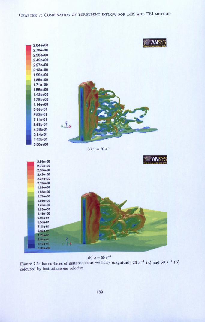
CHAPTER 7: COMBINATION OF TURBULENT INFLOW FOR LES AND FSI METHOD
2.840+00 2.70e+00 2.56e+00 2.429+00 2.279+00 2.13e+00 1.99e+00 1.85e+00 1.71 e+00 1.56e+00 1.42e+00 1.280+00 1.14e+00 9.95e-01 8.53e-01 7.11 e-01 5.68e-01 4.269-01 2.840-01 1.429-01 0.009+00
2.84e+00 2.70e+00 2.590+00
2.42. +00 2.270+00
2.134+00 1.990+00 1.850+00 1.71"+00 1.500+00 1.42e-t00
1.280+00 1.14e+00 9.950-01
9.530-01 7 110-01 5.680-01 4.269-01 2.849-01 1.420-01 0.000+00
a
:,.
(I)) w- 50s l
Figure 7.5: Iso surfaces of instantaneous vorticity magnitude 20 s-1 (a) and 50 s-1 (b) coloured by instantaneous velocity.
400P
189
(a)w=20s-1

CHAPTER 7: COMBINATION OF TURBULENT INFLOW FOR LES AND FSI METHOD
2.849+00 2.89e+00 2.55e+00
ý' ' 2 410x00 " 22l e+ 2130-+00
" i-' 1.990+00 tf
1.84e+00 � 1.700+00 1.569+00 1.42e+00 1.289+00 1.130+00, 9.939-01 8519-01 709o- O1
5.67e-O1 4 259-01 284a-01 *
1.429-01 y X 0000+00
Figure 7.6: Iso surface of a topological vortex indicator H = -30, indicator of the rotational structures in the flow. The tubular structures by the front edges of the building can be observed.
200. «02 1J
1.900+02
ý'..,
100«01 301e-03
Figure 7.7: ( ....... ........... . .. - ,,., �.. .. � i, jIhU l gear the ground
atz=L/10.
190

CHAPTER 7: COMBINATION OF TURBULENT INFLOW FOR LES AND FSI METHOD
and z= 2h/3 on a horizontal line. These coefficients of pressure are mean values ob-
tained from statistical averaging (definition in Section 4.4, p. 105). The reference velocity
used to compute the pressure coefficients is the velocity at z= h/3 for (a), and z= 2h/3
for (b) far from the building. The reference pressure is taken to be the operating pres-
sure far from the building. The results are compared to experimental data published
for the CAARC building. For the results at z= h/3, the CFD results are compared
to wind tunnel results from Golfger and Milford (1988), who tested two levels of lon-
gitudinal turbulence. The results at z= 2h/3 are compared to experimental results
from Melbourne (1980) (City University and Monash University) and to results from
Tanaka and Lawen (1986) (University of Ottawa). Since the width to length ratio is 1.5
for the CAARC building and 2 for the building of interest here, the experimental results
are scaled. The first graph compares the CFD results to experimental results done in
"low" and "high" turbulence wind tunnels. From the comparison, Cp is overpredicted on
the front face, giving even larger values than the lowest turbulent case of the experimen-
tal data. This would tend to indicate that the "low" turbulent flow in the experiments
was still more turbulent than the present simulation. The same reason can explain the
underprediction of Cp on the back face. The predictions are better on the side face,
which could be explained by the fact that the flow on the side face is dominated by
the recirculation zone after the front edge of the building, so the flow is less dependent
on the oncoming turbulence. The second graph compares the CFD results of Cp at
z= 2h/3 with experimental data from various research groups (CAARC). Generally,
the pressure coefficient is larger on the front face at z= 2h/3 than at z= h/3, which
is confirmed by the contours of the static pressure in Figure 7.9. The maximal pressure
can be observed at about z= 4h/5. On the front face, the maximum relative error is
reached in the middle of the section and is equal to about 11%. The results are in good
agreement with experiments on the side and back faces. On the side and back faces, Cp
is over predicted by about 11%.
The longitudinal and transversal response of the top of the building is shown in Figure
7.10 for the reduced velocity u/(nW) = 2.2. The amplitude of longitudinal response
191

CHAPTER 7: COMBINATION OF TURBULENT INFLOW FOR LES AND FSI METHOD
O LES 0.8 + exp low Curb
+* exil high turb
..... .... ................:. . 0.6 OO o! "º0
c +O O+
0.2- 0
0 ....... . ...........
c -0.2
.... i.... ý' s
-0.6 0 O
-0.8
012345 x'
(a) "exp" refers to experimental results from Golfger and Milford (1988)
1'
012345 X
(b) "exp" refers to experimental results from Melbourne (1980); Tanaka and Lawen (1986)
z=2h/3
5
z1�3
(c)
Figure 7.8: Distribution of pressure coefficient along an horizontal line at z= h/3 (a)
and z= 2h/3 (b) as shown in (c). LES results compared to experimental data extracted from Braun and Awruch (2009). 192

CHAPTER 7: COMBINATION OF TURBULENT INFLOW FOR LES AND FSI METHOD
2.00 1.90 1.80 1.70 1.60 1.50 1.40 1.30 1.20 1.10 1.00 0.90 0.80 0.70 0.60 0.50 0.40
Y- -X 0.30 0.20 0.10 0.00
Figure 7.9: Contours of the static pressure distribution on the front face of the building.
is about 10 times larger than the amplitude of the transversal response. Structural
damping causes the longitudinal response to decrease with time.
The transversal response is relatively small, which can be explained by the fact the
reduced velocity is far from the region of "lock-in", or in other words, the frequency of
the oscillating lift acting on the building remains far from the natural frequency of the
building, for which the building response would be maximal. The transversal response
is expected to be larger if the reduced velocity reaches 1.1 as seen in Chapter 5.
Figure 7.11 shows the trajectory covered by the roof center point of the building. The
reduced velocity being far from the critical reduced velocity, the trajectory does not
exhibit a predominant direction of motion.
7.5 Conclusions
This Chapter presented the results of a simulation combining the two tools developed in
previous chapters. The turbulent inflow generator and the fluid-structure coupling are
193

CHAPTER 7: COMBINATION OF TURBULENT INFLOW FOR LES AND FSI METHOD
E
0.02
........ ..................... ... 0.04- _.. ....:.. _..... 0.03-
g0
0
-0.02-
-0.03-
-0.04
-0.058 iZ345878 Sm. (a)
(b)
Figure 7.10: Response of the building (a) longitudinal response (b) transversal response.
0.01
1o -o. o1 ...
-0.02
-0.03
-Ö02 0 0.02 a
0.04 wIvAnd0.06
ý 0.1 0.12 0.14
Figure 7.11: Trajectory covered by the roof center point.
194
-V' 02488 10 12 lima (s)
(a)

CHAPTER 7: COMBINATION OF TURBULENT INFLOW FOR LES AND FSI METHOD
used in combination in a fairly heavy simulation, which involves a very large number of
cells to reach the minimum level of refinement required by LES. The mesh had also to
be fine enough to maintain the turbulent structures that were injected at the inlet with
the turbulent inflow generator.
The results, in terms of mean and rms velocities, showed good agreement with ESDU.
Integral length scales in the ABL were reproduced with confidence. The 3D features of
the wind flow, shown with iso surfaces of vorticity and contours of vorticity, presented a
good qualitative picture of the wind flow. The quantitative comparisons of the pressure
coefficients on the building showed good agreement with wind tunnel testing of the
CAARC building. In terms of the response, since only one reduced velocity could be
tested, only qualitative conclusions could be drawn. Chapter 5 demonstrated that the
code could successfully couple fluid and structure's motion in the transversal direction,
but the results of this chapter show that the structure can also be coupled with the wind
flow in the longitudinal direction.
To conclude this chapter, a framework has been established to numerically study the
wind flow around tall buildings and their response to wind loading. If more computing
resources become available, the framework could be used to produce a more systematic
numerical study of the response of a tall building to wind loading, by testing a range of
reduced velocity.
195

Chapter 8
Conclusions and
Recommendations
8.1 Summary
The main goal was to assess the the ability of commercial CFD codes to model the
wind flow around a high-rise building - specifically the coupled dynamic response of the
building to turbulent wind loading - by bringing together existing tools, thus establishing
a framework for modelling of building response to wind loading within a turbulent ABL.
In order to meet the main objective three intermediate objectives were set. The first was
to develop a tool for coupling the fluid and the structure, within the framework of the
FLUENT code. The structural solver was contained in code attached to the CFD code in
the form of user-defined functions. The fluid-structure coupling was then used to model
a cantilever allowed to move in the transversal direction only. Turbulence modelling
here was by means of an unsteady hybrid RANS-LES model that could reproduce small
scale wake effects and large scale features, such as vortex shedding. The structure's
response to vortex shedding in the wake was seen through the aeroelastic phenomenon
of "lock-in", which occurs when the vortex shedding frequency is close to the natural
frequency of the building. More precisely, "lock-in" was found to occur for a reduced
196

CHAPTER 8: CONCLUSIONS AND RECOMMENDATIONS
velocity of about 1.1, in agreement with the literature on "lock-in" phenomenon for
rectangular cylinders and more recent publications on tall buildings.
The second intermediate objective was to investigate and apply a method for generating
turbulent inflow for LES. It was shown in Chapter 2 that not only are wake effects of
importance when predicting the response of tall buildings to wind loading, but also that
the turbulence in the oncoming wind is of great importance. Upstream turbulence can
produce a significant response of the structure if the natural frequency of the building is
in the range of the dominant frequencies in the wind spectrum. For this reason, it was
decided to adopt LES instead of the hybrid RANS-LES. However, LES requires a realistic
turbulent inflow at the inlet of the domain. The option to use a precursor simulation to
produce the appropriate turbulent inflow was considered too computationally expensive,
and it was decided to produce a turbulent inflow synthetically, using a method developed
by Xie and Castro (2008). The method for generating synthetic turbulent inflow was
tested in an empty domain to determine the main statistical properties of the generated
inflow, both on the inlet plane and as the flow moves through the fetch. It was found that
it was possible to generate turbulent inflow at the inlet with predetermined statistical
properties and that these properties were maintained throughout the domain.
Finally, in order to meet the third intermediate objective, the turbulent inflow genera,
for and the fluid-structure coupling tool were brought together. In this final stage, the
building was allowed to bend in both the along-wind and transversal directions. The
structure was found to respond to wake effects (vortex shedding) but also to the wind
gusts. In addition, results of the LES simulation in terms of the pressure distribution
on the building, velocity profiles, turbulence, flow field around the building, and more
particularly in the wake were shown to be in good agreement with experimental data.
The main achievement of Chapter 7 was to establish a framework to numerically study
the wind flow around tall buildings and their response to wind loading, and to demon-
strate the ability of commercial CFD to model the wind flow around a high-rise building,
addressing the main objective of this thesis.
197

CHAPTER 8: CONCLUSIONS AND RECOMMENDATIONS
In addition, a complementary study was done to challenge the current recommendations
for the size of the computational domain for studying the wind flow around tall buildings.
It was found that the size of the domain could be greatly reduced. This finding was then
used in the later parts of the work, allowing us to achieve more efficient simulations in
which the overall domain size could be reduced and the number of cells could be increased
in key regions, such as the wake of the building.
8.2 Critical appraisal
Firstly, the framework that has been developed requires more testing. In the first in-
stance, the sensitivity of the model to changes in inlet velocity, turbulence intensity,
structural stiffness and damping and many other variables needs to be investigated.
Secondly, it needs to be validated against full scale or wind tunnel experiments on an
aeroelastic building. Both these investigations will require large amounts of computa-
tional time, which were beyond the scope of the present work.
Secondly, the structural solver was shown to work for individual modes, and it would
be a trivial exercise to extend it to secondary and torsional modes.
Then, in order to make the method directly applicable to civil engineering, the region
containing the building would need to be able to rotate to test a number of wind direc-
tions, as suggested by Morvan et a1. (2007).
As for the method to generate turbulent inflow, it is not computationally expensive,
at least for the applications concerned by this thesis. However, if the computational
cost becomes an issue (for larger inlets, longer periods of time... ), the method could
be linked to methods such as wavelet reconstruction, which is a method that allows
the reproduction of non-linearity in the wind. For example, one could produce the
turbulent inflow with the method presented here, run it once or twice though the domain,
and use the wavelet reconstruction method to reproduce and extend the wind outflow,
that could then be used as a new inflow. The combination could potentially be more
computationally efficient.
198

CHAPTER 8: CONCLUSIONS AND RECOMMENDATIONS
Finally, it was demonstrated that given an input of Reynolds stresses and integral length
scales, it was possible to generate turbulent inflow for LES. However, more and more
work seems to be done in linking micro scale models to larger scale meteorological scale
models, which could be of interest in further work (Mochida et al., 2010).
8.3 Conclusions
The first conclusion that can be drawn from this thesis is that commercial CFD can
be suitably adapted to model the wind flow around a high-rise building, and more
specifically, it can be applied to model the coupled dynamic response of the building
to turbulent wind loading. The second conclusion addresses the issue of computational
domain sizes. The work that has been done as part of this thesis demonstrated that the
current recommendations on domain sizes are inappropriate for tall buildings, and new
recommendations were defined. Finally, it was shown that a synthetic method based on
inverse Fourier transforms can be successfully used to generate turbulent inflow.
8.4 Further work
" Test the sensitivity of the model to change in inlet velocity, turbulent intensity,
structural stiffness and damping.
" Include secondary modes and torsional modes.
" Modify the FSI code so it can be restarted at anytime (if it crashes for example).
At the moment, if the run crashes for any reason, it has to be restarted from when
the building is released.
" Define a cylindrical zone around the rigid zone already defined around the building.
This cylindrical zone could then be rotated, allowing a range of wind directions to
be tested.
199

CHAPTER 8: CONCLUSIONS AND RECOMMENDATIONS
" Use the synthetic turbulent inflow generator in combination with a wavelet recon-
struction approach.
9 Linking to larger scale meteorogical models.
200

Bibliography
ANSYS. ANSYS-Fluent 12.0 User Manual, ANSYS Inc. Fluent. Southpointe, Canons-
burg PA, USA, 2009.
Carla Antoci, Mario Gallati, and Stephano Sibilla. Numerical simulation of fluid-
structure interaction by sph. Computers and Structures, 85: 879-890,2007.
J. Baldyga and J. R. Bourne. Fluid mechanical approach to turbulent mixing and chem-
ical reaction. Chemical Engineering Communications, 28: 231-281,1984.
P. W. Bearman. Vortex shedding from oscillating bluff bodies. Annu. Rev. Fluid Mech.,
16: 195-222,1984.
Prof. A. A. Becker. Finite Element Analysis for Engineers, Course Lecture Notes. Uni-
versity of Nottingham, 2008.
Girma Bitsuamlak and Emil Simiu. Cfd's potential applications: a wind engineering
perspective. In Proceedings of the Fifth International Symposium on Computational
Wind Engineering, Chapel Hill, North Carolina, USA, 2010.
Bert Blocken, Ted Stathopoulos, and Jan Carmeliet. Cfd simulation of the atmospheric
boundary layer: wall function problems. Atmospheric Environment, 41: 238-252,2007.
Alexdrandre Luis Braun and Armando Miguel Awruch. Aerodynamic and aeroelastic
analysis on the caarc standard tall building model using numerical simulation. Com-
puters and Structures, 87: 564-581, march 2009.
201

BIBLIOGRAPHY
M. Breuer, B. Kniazev, and M. Abel. Development of wall models for les of separated
flows using statistical evaluations. Computers and Fluids, 36: 817-837,2007.
M. Breuer, B. Jaffrezic, and K. Arora. Hybrid les-rans technique based on a one-equation
near wall model. Theor. Comput. Fluid Dyn., 22: 157-187,2008.
R. Buccolieri and S. Di Sabatino. Flow and pollutant dispersion in urban arrays for
the standardization of CFD modelling practise. In Proceedings of the 11th Conference
on Harmonisation within Atmospheric Dispersion Modelling for Regulatory Purposes,
Cambridge, July, 2007.
Tony Burton, David Sharpe, Nick Jenkins, and Ervin Bossanyi. Wind Energy Handbook.
John Wiley & Sons, 2002.
Ian P. Castro and J. M. R. Graham. Numerical wind engineering: the way ahead? In
Proceedings of The Institution of Civil Engineering Structures & Buidlings, pages
275-277, August 1999.
Ray W. Clough and Joseph Penzien. Dynamics of Structures, Second Edition. McGraw-
Hill book Co., 1993.
N. J. Cook. The designer's guide to wind loading of building structures, Part 1. Butter-
worth, 1992.
J. Counihan. Adiabatic atmospheric boundary layers: A review and analysis of data
from the period 1880-1972. Atmos. Env., 9: 871-905,1975.
Jason J. Dale, D. B. Spalding, A. E. Hold, and M. G. Armstrong. Fluid structure interac-
tion through simultaneous calculation of velocity and displacement. PVP, Emerging
Technologies in Fluids, Structures, and Fluid/Structures Interactions, 446-2: 129-139,
2002.
A. G. Davenport. How can we simplify and generalize wind loads. Journal of Wind
Engineering and Industrial Aerodynamics, 54/55: 657-669,1995.
202

BIBLIOGRAPHY
Alan Garnett Davenport. The application of statistical concepts to the wind loading of
structures. In Proceedings of The Institution of Civil Engineers. The Institution of
Civil Engineers, August 1961.
L. Davidson and M. Billson. Hybrid les-rans using synthesized turbulent fluctuations
for forcing in the interface region. Int. J. of Heat and Fluid Flow, 27: 1028-1042,2006.
L. Davidson and S. H. Peng. Hybrid les-rans modelling: a one equation sgs model
combined with a k-w model for predicting recirculating flows. Int. J. Nurner. Meth.
Fluids, 43: 1003-1018,2003.
J. Donea, Antonio Huerta, H-Ph. Ponthot, and A. Rodriguez-Ferran. Arbitrary La-
grangian - Eulerian Methods, chapter 14, pages 1-25. John Wiley & Sons, 2004.
P. Duchene-Marullaz. Effects of high roughness on the characteristics of turbulence in
the case of strong winds. In Proceedings of the Fifth International Conference on
Wind Engineering, 1980.
Clas Dyrbye and Svend Ole Hansen. Wind loads on structures. John Wiley & Sons,
1997.
ESDU 85020. Esdu 85020: Characteristics of atmospheric turbulence near the ground,
part ii: single point data for strong winds (neutral atmosphere). Technical report,
1985, revised in 1990.
ESDU 86010. Characterisation of atmospheric turbulence near the ground, part iii:
Variations in space and time for strong winds (neutral atmosphere). Technical report,
1986, revised in 2001.
Robert E. Eskridge and J. C. R. Hunt. Highway modeling. part i: Prediction of velocity
and turbulence fields in the wake of vehicles. Journal of Applied Meteorology, 18:
387-, 400,1979.
Ralph Evins. Fds assessment. Technical report, Buro Happold, 2007.
203

BIBLIOGRAPHY
C. Farhat and M. Lesoinne. Two efficient staggered algorithms for the serial and paral-
lel solution of three-dimensional nonlinear transient aeroelastic problems. Computer
methods in applied mechanics and engineering, 182: 499-515,2000.
C. Farhat, M. Lesoinne, and N. Maman. Mixed explicit/implicit time integration of
coupled aeroelastic problems: three field formulation, geometric conservation and
distributed solution. Int. J. Numer. Meth. Fluids, 21: 807-35,1995.
C. Farhat, G. van der Zee Kristoffer, and P. Geuzaine. Provably second-order time-
accurate loosely-coupled solution algorithms for transient nonlinear computational
aeroelasticity. Computers methods in applied mechanics and engineering, 195: 1973-
2001,2006.
A. A. Fediw, M. Nakayama, K. R. Cooper, Y. Sasaki, S. Resende-Ide, and S. J. Zan.
Wind tunnel study of an oscillating tall building. Journal of Wind Engineering and
Industrial Aerodynamics, 57: 249-260,1995.
R. M. Franck and R. B. Lazarus. Mixed eulerian-lagrangian method: vol. 3: Fundamental
methods in hydrodynamics. In B. Alder, S. Fernbach, and M. Rotenberg, editors,
Methods in Computational Physics, pages 47-67,1964.
J. Ranke. Introduction to the prediction of wind loads on buildings by computational
wind engineering (CWE). In T. Stathopoulos and C. C. Baniotopoulos, editors, Wind
Effects on Buildings and Design of Wind-sensitive Structures, chapter 3, pages 67-
103. SpringerWien, New York, 2007.
J. Franke, C. Hirsch, A. G. Jensen, H. W. Krüs, M. Schatzmann, P. S. Westbury, S. D.
Miles, J. A. Wisse, and N. G. Wright. Recommendations on the use of CFD in wind
engineering. In J. P. A. J. van Beeck, editor, COST Action C14: Impact of Wind and
Storm on City Life and Built Environment, pages C. 1.1-C. 1.11. von Karman Insitute
for Fluid Dynamics, 2004.
J. Franke, A. Hellsten, Schlunzen, and B. Carissimo. Best practice guide for the CFD
204

BIBLIOGRAPHY
simulation of flows in the urban environment. In COST Action 732: Quality assurance
and improvement of microscale meteorological models, 2007.
S. Pu, B. E. Launder, and D. P. Tselepidakis. Accomodating the effects of high strain
rates in modelling the pressure-strain correlation. Technical report, UMIST Mech.
Eng. Dept. Report. TFD/87/5,1987.
J. R Garrat. The Atmospheric Boundary Layer. Cambridge University Press, 1992.
M. Germano, U. Piomelli, P. Moin, and W. H. Cabot. A dynamic subgrid scale eddy
viscosity model. Phys. Fluids A, 3: 1760-1765,1991.
J. H. Gerrard. The mechanics of the formation region of vortices behind bluff bodies. J.
Fluid Mech., 25: 401-413,1966.
Anvar Gilnianov and Sumanta Acharya. A hybrid immersed boundary and material
point method for simulating 3d fuid-structure interaction problems. International
Journal for Numerical Methods in Fluids, 56: 2151-2177,2007.
AM Golfger and RV Milford. Sensitivity of the CAARC standard building model to
geometric scale and turbulence. Journal of Wind Engineering and Industrial Aerody-
namics, 31(1): 105-123,1988. ISSN 0167-6105.
C. Gorle, J. van Beeck, P. Raxnbaud, and G. Tendeloo. Cfd modelling of small particle
dispersion: The influence of the turbulence of the turbulence kinetic energy in the
atmospheric boundary layer. Atmospheric Environment, 43: 673-681,2009.
Kemal Hanjalic and Sasa Kenjeres'. Some developments in turbulence modelling for
wind and environmental engineering. Journal of Wind Engineering and Industrial
Aerodynamics, 96: 1537-1570,2008.
D. M. Hargreaves and N. Wright. On the use of the k-e model in commercial cfd software
to model the neutral atmospheric boundary layer. Journal of Wind Engineering and
Industrial Aerodynamics, 95: 355-369,2007.
205

BIBLIOGRAPHY
R. I. Harris. The macrometeorological spectrum -a preliminary study. Journal of Wind
Engineering and Industrial Aerodynamics, 96: 2294-2307,2008.
R. I. Harris and D. M. Deaves. The structure of strong winds. In Proceedings of the
Seminar on Wind Engineering in the Eighties, 1980.
E. L. Houghton and N. B. Carruthers. Wind forces on buildings and structures: an in-
troduction. Edward Arnold, 1976. ISBN 0713133619.
R. P. Hoxey, P. J. Richards, and J. L. Short. A6m cube in an atmospheric boundary layer
flow part 1. full-scale and wind-tunnel results. Wind and Structures, 5(2-4): 165-176,
2002.
S. Huang, Q. S. Li, and S. Xu. Numerical evaluation of wind effects on a tall steel
building by cfd. Journal of Constructional Steel Research, 63: 612-627,2007.
T. Ishihara and K. Hibi. Turbulent measurements of the flow field around a high-rise
building. J. Wind Eng. Japan, 76: 55-64,1998.
M. Kato and B. E. Launder. The modeling of turbulent flow around stationary and
vibrating square cylinders. Prep. of 9th Symp. On Turbulent shear flow, 157: 10-4-1-
6,1993.
W. -W. Kim and S. Menon. Application of the localized dynamic subgrid-scale model to
turbulent wall-bounded flows. Technical Report AIAA-97-0210, American Institute of
Aeronautics and Astronautics, 35th Aerospace Sciences Meeting, Reno, NV,, January
1997.
M. Klein, A. Sadiki, and J. Janicka. A digital filter based generation of inflow data for
spatially developing direct numerical simulation or large eddy simulation. J. Comp.
Phys., 186: 652-665,2003.
A. N. Kolmogorov. The local structure of turbulence in incompressible viscous fluid for
very large reynolds numbers. In Dokl. Akad. Nauk SSSR, volume 30, pages 9-13,
1941.
206

BIBLIOGRAPHY
Ulrich Küttler and Wolfgang A. Wall. An approach for parallel fluid-structure interaction
on unstructured meshes. In Proceedings of the 13th European PVM/MPI user's group
meeting, Bonn, Germany, September 2006.
B. E. Launder and D. B. Spalding. The numerical computation of turbulent flows. Com-
put. Methods Appl. Mech. Eng., 3: 269-289,1974.
P. L'Ecuyer. Efficient and portable combined random number generators. Communica-
tion of the ACM, 31: 742-774,1988.
S. Lee, S. K. Lele, and P. Moin. Simulation of spatially evolving turbulence and the
applicability of taylors hypothesis in compressible flow. Phys. Fluids A, 4: 1521-1530,
1992.
Hee Chang Lim, T. G. Thomas, and Ian P. Castro. Flow around a cube in a turbulent
boundary layer: Les and experiment. Journal of Wind Engineering and Industrial
Aerodynamics, 97: 96-109,2009.
E. Longatte, Z. Bendjeddou, V. Verreman, and M. Souli. Comparison of strong and
partitioned fluid structure code coupling methods. In Proceedings of ASME 2005
Pressure Vessels and Piping Division Conference, Denver, Colorado, USA, July 2005.
Thomas S. Lund. Generation of turbulent inflow data for spatially-seveloping boundary
layer simulations. Journal of Computational Physics, 140: 233-258,1998.
WH Melbourne. Comparison of measurements on the CAARC standard tall building
model in simulated model wind flows. Journal of Wind Engineering and Industrial
Aerodynamics, 6(1-2): 73-88,1980. ISSN 0167-6105.
P. Mendis, T. Ngo, N. Haritos, A. Hira, B. Samali, and J. Cheung. Wind loading on
tall buidlings. EJSE Special Issue: Loading on Structures, pages 41-54,2007.
A. Mochida, S. Murakami, M. Shoji, and Y. Ishida. Numerical simulation of flowfield
around texas tech building by large-eddy simulation. Journal of Wind Engineering
and Industrial Aerodynamics, 46/47: 455-460,1993.
207

BIBLIOGRAPHY
A. Mochida, Y. Tominaga, S. Murakami, R. Yoshie, T. Ishihara, and R. Ooka. Compar-
ison of various k-epsilon models and dsm applied to flow around a high-rise building -
report on aij cooperative project for cfd prediction of wind environment -. Wind and
Structures, 5(2-4): 227-244,2002.
A. Mochida, S. Iizuka, Y. Tominaga, and I. Yu-Fat Lun. Up-scaling cwe models to
include mesoscale meteorological influences. In In: the Fifth International Symposium
on Computational Wind Engineering, Chapel Hill, North Carolina, USA, May 23-27,
2010.
H. P. Morvan, P. Stangroom, and N. G. Wright. Automated CFD analysis for multiple
directions of wind flow over terrain. Wind and Structures, 10(2): 99-120,2007. ISSN
1226-6116.
S. Murakaini. Current status and future trends in computational wind engineering.
Journal of Wind Engineering and Industrial Aerodynamics, 67&68: 3-34,1997.
S. Murakami. Overview of turbulence models applied in cwe-1997. Journal of Wind
Engineering and Industrial Aerodynamics, 74-76: 1-24,1998.
S. Murakami and A. Mochida. On turbulent vortex shedding flow past 2d square cylinder
predicted by cfd. Journal of Wind Engineering and Industrial Aerodynamics, 54-55:
191-211,1995.
S. Murakami, A. Mochida, K. Kondo, Y. Ishida, and Tsuchiya. Development of new
k-epsilon model for flow and pressure fields around bluff body. Journal of Wind
Engineering and Industrial Aerodynamics, 67&68: 169-182,1994.
B. Neammanee, S. Sirisumrannukul, and S. Chatratana. Development of a wind turbine
simulator for wind generator testing. International Energy Journal, 8: 21-28,2007.
N. V. Nikitin, F. Nocaud, B. Wasistho, K. D. Squires, and P. R. Spalart. An approach to
wall modelling in large-eddy simulations. Phys. Fluids, 12: 1629-1632,2000.
208

BIBLIOGRAPHY
W. F. Noh. Cel: a time dependent two space-dimensional, coupled eulerian lagrangian
code. In Methods in Computational Physics, volume 3, page 117. Academic Press.
New York, 1964.
Atsushi Okajima. Strouhal numbers of rectanguair cylinders. Journal of Fluid Mechan-
ics, 123: 379-398,1982.
S. V. Patankar and D. B. Spalding. A calculation procedure for heat, mass and momentum
transfer in three-dimensional parabolic flows. Int. J. Heat Mass Transfer, 15: 1787,
1972.
C. S. Peskin. Numerical analysis of blood flow in the heart. Journal of computational
physics, 25(3): 220-252,1977.
S. Piperno, C. Farhat, and B. Larrouturou. Partitioned procedures for the transient
solution of coupled aeroelastic problems. Comput. Methods Appl. Mech. Eng., 124:
79-711,1995.
Stephen B. Pope. Turbulent Flows. Cambridge University Press, 2000.
F. Porte-Agel, C. Meneveau, and M. B. Parlange. A scale-dependent dynamic model for
large edd simulation: application to a neutral atmospheric boundary layer. Journal
of Fluid Mechanics, 415: 261-284,2000.
Willian H. Press, Saul A. Teukolsky, Willian T. Vetterling, and Brian P. Flannery.
Numerical Recipes in C: The art of Scientific Computing, Second Edition, volume
Chapter 7. Random Numbers. Cambridge University press, 1992.
T. Prevezer, J. Holding, A. Gaylard, and R. Palin. Bluff body asymmetric flow phe-
nomenon - real effect or solver artefact? Wind & Structures, 5: 359-368,2002.
J. Revuz, DM Hargreaves, and J. Owen. Numerical simulation of the dynamic wind
loading on and response of tall buildings. In Proceedings of the Proceedings of the fifth
European and African Conference on Wind Engineering, Florence, Italy, 2009.
209

BIBLIOGRAPHY
G. M. Richards, R. P. Hoxey, and L. J. Short. Wind pressures on a6m cube. Journal of
wind Engineering and Industrial Aerodynamics, 89: 1553-1564,2001.
P. J. Richards and R. Hoxey. Appropriate boundary conditions for computational wind
engineering models using the k-E turbulence model. J. Wind Eng. Ind. Aerodyn, 46
& 47: 145-153,1993.
P. J. Richards and A. D Quinn. A6m cube in an atmospheric boundary layer flow part
2. computational solutions. Wind and Structures, 5(2-4): 177-192,2002.
Silvana Di Sabatino, Alexander Baklanov, John Bartzis, Ruwim Berkowicz, Riccardo
Buccolieri, Ana Margarida Costa, George Efthimiou, Jrg Franke, Matthias Ketzel,
Bernd Leitl, Roman Nuterman, Helge Rrdam Olesen, and Richard Tavares. Analyses,
critical issues and outcome from cost732 cfd evaluation exercise. In Proceedings of
the Fifth International Symposium on Computational Wind Engineering, Chapel Hill,
North Carolina, USA, 2010.
Peter Sachs. Wind forces in Engineering. Pergamon press, 1978.
R. Sankaran and D. A. Paterson. Computation of rain falling on a tall rectangular
building. J. Wind Eng. Ind. Aerodyn., 72: 127-136,1997.
Inanc Senocak, Andrew S. Ackerman, Michael P. Kirkpatrick, David E. Stevens, and
Nagi N. Mansour. Study of near-surface models for large-eddy simulations of a neu-
trally stratified atmospheric boundary layer. JBoundary-Layer Meteorology, 124: 405-
424,2007.
E. Simiu and R. H. Scanlan. Wind effects on structures. Wiley-Interscience, 1986.
A. K. Slone, K. Pericleous, C. Bailey, and M. Cross. Dynamic fluid-structure interaction
using finite volume unstructured mesh procedures. Computers and Structures, 80:
371-390,2002.
A. K. Slone, K. Pericleous, C. Bailey, M. Cross, and C. Bennett. A finite volume un-
structured mesh approach to dynamic fluid-structure interaction: an assessment of
210
BIBLIOGRAPHY
the challenge of predicting the onset of flutter. Applied Mathematical Modelling, 28:
211-239,2004.
J. Smagorinsky. General circulation experiments with the primitive equations. i. the
basic experiment. Month. Wea. Rev., 91: 99-164,1963.
E. S. P. So, A. T. Y. Chan, and A. Y. T. Wong. Large-eddy simulations of wind flow and
pollutant dispersion in a street canyon. Atmos. Env., 39: 3573-3582,2005.
P. Spalart. Young-person's guide to detached-eddy simulation grids. Technical Report
CR-2001-211032, NASA, July 2001.
C. G. Speziale, , S. Sarkar, and T. B. Gatski. Modelling the pressure-strain correlation of
turbulence: and invariant dynamical system approach. J. Fluid Mech., 227: 245-272,
1991.
Theodore Stathopoulos. Computational wind engineering: Past achievements and future
challenges. Journal of Wind Engineering and Industrial Aerodynamics, 67-68: 509-532,
1997.
S. Swaddiwudhipong and M. S. Khan. Dynamic response of wind-excited building using
cfd. Journal of Sound and Vibration, 253(4): 735-754,2002.
GR Tabor and MH Baba-Ahmadi. Inlet conditions for large eddy simulation: A review.
Computers £9 Fluids, 39(4): 553-567,2010. ISSN 0045-7930.
H. Tanaka and N. Lawen. Test on the CAARC standard tall building model with a
length scale of 1: 1000. Journal of Wind Engineering and Industrial Aerodynamics,
25(1): 15-29,1986. ISSN 0167-6105.
L. Temmerman, M. A. Leschziner, C. P. Mellen, and J. Frohlich. Investigation of wall-
function approximations and subgrid-scale models in large eddy simulation of sepa-
rated flow in a channel with streamwise periodic constrictions. Int. J. of Heat and
Fluid Flow, Turbulence and Combustion, 24: 157-180,2003.
211

BIBLIOGRAPHY
L. Temmerman, M. Hadiiabdic, M. A. Leschziner, and K. Hanjalic. A hybrid two-layer
urans-les approach for large eddy simulation at high reynolds numbers. Int. J. of Heat
and Fluid Flow, 26: 173-190,2005.
F. Tessicini, L. Temmerman, and M. A. Leschziner. Approximate near-wall treatments
based on zonal and hybrid rans-les methods for les and high reynolds numbers. Int.
J. of Heat and Fluid Flow, 27: 789-799,2006.
F. Tessicini, N. Li, and M. A. Leschziner. Large-eddy simulation of three-dimensional
flow around a hill-shaped obstruction with a zonal near-wall approximation. Int. J.
of Heat and Fluid Flow, 28: 894-908,2007.
T. G. Thomas and J. J. R. Williams. Generating a wind environment for large eddy simu-
lation of bluff body flows. Journal of Wind Engineering and Industrial Aerodynamics,
82: 189-208,1999.
Y. Tominaga, A. Mochida, R. Yoshie, H. Kataoke, T. Nozu, M. Yoshikawa, and T. Shira-
sawa. AIJ guidelines for practical applications of CFD to pedestrian wind environment
around buildings. J. Wind. Eng. Ind. Aerodyn., 96: 1749-1761,2008.
Isaac van der Hoven. Power spectrum of horizontal wind speed in the frequency range
from 0.0007 to 900 cycles per hour. J. Meteor., 14: 160-164,1957.
H. K. Versteeg and W. Malalasekera. An Introduction to Computational fluid dynamics,
The Finite Volume Method. Pearson Education, 2007.
R. L. Wardlaw and G. F. Moss. A standard tall building model for the comparison of
simulated natural winds in wind tunnels. Technical report, Supplement by Common-
wealth Advisory Aeronautical Research Council, 1971.
M. Watakabe, M. Ohashi, H. Okada, Y. Okuda, Y. Okuda, H. Kikitsu, S. Ito, Y. Sasaki,
K. Yasui, K. Yoshikawa, and M. Tonagi. Comparison of wind pressure measurements
on tower-like structure obtained from full-scale observation, wind tunnel test, and the
CFD technology. J. Wind Eng. Ind. Aerodyn., 90: 1817-1829,2002.
212

BIBLIOGRAPHY
C. H. K. Williamson and R. Govardhan. A brief review of recent results in vortex-induced
vibrations. Journal of Wind Engineering and Industrial Aerodynamics, 96: 713-735,
2008.
N. G. Wright and G. J. Easom. Non-linear k-e turbulence model results for flow over a
building at full scale. Apl. Math. Modelling, 27: 1013-1033,2003.
Y. Wu, X. Sun, and S. Shen. Computation wind-structure interaction on tension
structures. Journal of Wind Engineering and Industrial Aerodynamics, page doi:
10.1016/j. jweia. 2008.02.043,2008.
W. Xiang and H. Wang. Discussion on grid size and computational domain in CFD
modelling of pedestrian wind environment around buildings. J. Civ. Eng. Arch., 2(1):
8-14,2008.
Zhenh-Tong Xie and Ian P. Castro. Efficient generation of inflow conditions for large
eddy simulation of street-scale flows. Flow, Turbulence and Combustion, 81(3): 449-
470, October 2008.
V Yakhot, S. A. Orszag, S. Thangam, T. B. Gatski, and C. G. Speziale. Development of
turbulence models for shear flows by a double expansion technique. Physics of Fluids
A, 4: 1510-1520,1992.
W. Yang, H. An, M. Gu, and S. Chen. Applicationof new inflow boundary conditions for
modelling equilibrium atmosphere boundary layer in rans-based turbulence models.
In Proceedings of International Conference on Wind Engineering, 2007.
Yi Yang, Ming Gu, Suqin Chen, and Xinyang Jin. New inflow boundary conditions for
modelling the neutral equilibrium atmospheric boundary layer in computational wind
engineering. Journal of Wind Engineering and Industrial Aerodynamics, 97: 88-95,
2009.
L. T. Zhang and M. Gay. Immersed finite element method for fluid-structure interaction.
Journal of Fluids and Structures, 23: 839-857,2007.
213

Appendices
214

Appendix A
The Arbitrary Lagrangian Eulerian formulation for mesh-fluid coupling
This appendix presents a kinematical description of the Arbitrary Lagrangian Eulerian
formulation, based on Donea et al. (2004).
Figure A. 1 illustrates the three frames of reference: Rx is the material configuration (X
is the material coordinate in the Lagrangian description), Rx the spatial configuration
(z is the spatial coordinate in the Eulerian description) and R. is the referential config-
uration. Theoretically, the referential configuration could be any configuration, but it
is usually seen as the mesh configuration. Therefore x is the computational coordinate.
One can express the mapping application from the computational to the spatial config-
uration:
4, : Rx x (to, tflnal[ -+ Rg x [t0, tfnal
(x, t) '--+ db (X, t) _ (x,
the transformation from the material configuration to the spatial configuration:
(p : Rx x [to, tfinal[ -4 R. x [t0, tfinal
(X, t) '--+
215

APPENDIX A: THE ALE FORMULATION FOR MESH-FLUID COUPLING
RX
(Q Ncýý
material
RX
spatial
'`X computational
Figure A. 1: Material, spatial and computational frames of reference and mapping trans- formations of the ALE method (after Donea et al. (2004)).
and the transformation from the computational domain to the material configuration:
-1 : Rx x [to, tfinai [ -+ RX x [to, tfinal [
(X, t) = (x, t)
The three applications are not independently defined, and the following composition of
mapping exists: (illustrated in Figure A. 1):
w_4o41-1
The gradients of each transformation can be expressed as matrices:
a_(x, c) 80 7), aý(x, t) __
v}' A02 a(x, t) oT a(x, t) ()T 1J 49(X, t) OT 1
wJ (.. ý
where v is the material velocity, which is the velocity of the particles evaluated in the
spatial frame of reference, b expresses the mesh velocity (the velocity of the computa-
tional frame evaluated in the spatial frame of reference) and w is the velocity of particle
216

APPENDIX A: THE ALE FORMULATION FOR MESH-FLUID COUPLING
evaluates in the computational frame of reference.
ax Ox aX IX (A. o. 3) V= - Ix, at IX, w= at
In a fully Lagrangian approach, there is no relative motion between the particles and the
mesh, which translated into: w =0 and v=Z. Whereas in a fully Eulerian approach,
the computational frame of reference and the spatial frame of reference coincide: v=
0andv=w
The differentiation of Equation (A. 0.1) leads to:
aýp(x, t) _
a4(x, t) aW-1(x, t) a(x, t) - a(x, t) a(x, t)
(A. 0.4)
If each terms is replaced by its definition (Equations (A. 0.2)), it leads to the definition
of the convective velocity c, which is the velocity between the material and the mesh:
ax C=V-V=-. W
X (A. 0.5)
The fundamental ALE equations are then obtained by replacing the velocity in the
spatial frame of reference v by the convective velocity c in the convective terms of the
continuity and momentum equations:
5Ix+c"vp =0 (A. 0.6)
p(; fix+(c. V)v)) = V"a+p9 (A. 0.7)
where p is the density, a the Cauchy stress tensor and g the gravity force vector. It
must be noted that in both equation the derivatives in the spatial frame of reference are
replaced by derivatives in the computational frame of reference. New terms related to
the mesh velocity v appear in the left hand side of each equation.
Finally, when considering fluid-structure interactions, the following boundary conditions
are applied at the interface: the velocity of the fluid and the structure (subscript s) must
217

APPENDIX A: THE ALE FORMULATION FOR MESH-FLUID COUPLING
coincide along the interface for a viscous fluid:
u= u9 continuity of displacement
v= v8 continuity of velocities
The integral forms of the equations of the ALE formulation can be found in Donea et al.
(2004)
218

Appendix B
UDF for fluid structure interactions
B. 1 Finite Element Method: openFEM
The FEM analysis is done using the open-source package openFEM1, which runs within
Matlab. The underlying ideas of Finite Element Analysis is to divide the domain into
small finite segments, and the behaviour of each of these elements is described by the
displacements of the elements and the material laws. All elements are assembled to-
gether and the requirements of continuity and equilibrium are satisfied between the
neighbouring elements. Provided that the boundary conditions of the actual problem
are satisfied, a unique solution can be obtained to the overall system of linear algebraic
equations. (Becker, 2008)
B. 2 Running the flow solver ANSYS-Fluent with fluid- structure interactions
The structural properties and the mode shapes of the cantilever are obtained from the
FEM analysis. Two files are output at the end of the FEM analysis:
1. "dyn_pmperties. txt": contains the structural properties of the structure:
" 1, A, rho: the height, the cross section and the density of the material respec- The documentation about openFEM can be found at http: //wvw. sdtoole. com/openfem/, it is
distributed under the LGPL license.
219
APPENDIX B: PROGRAM FOR FLUID STRUCTURE INTERACTIONS
tively,
" EIx, Ely: the flexural stiffness in the along wind and the cross-wind directions
respectively,
" Mnx, Mny: the generalised mass in the along-wind and the cross-wind direc-
tions respectively,
" Knx, Kny: the generalised stiffness in the along-wind and the cross-wind
directions respectively, and
" wnx, wny: the natural frequency in the along-wind and the cross-wind direc-
tions respectively.
2. "mode-shapes. txt" : contains the mode shapes information of the first mode in each
direction.
B. 3 The FSI program (the UDF): functions and Macros
As explained in section 5.3.3, the FSI program is a User-Defined Function that is called
by the flow solver. The UDF is composed of a number of auxiliary functions, and
MACROS, which allow the user to access and modify solver data.
B. 3.1 Auxiliary functions in the UDF
The following auxiliary functions are used in the UDF:
1. Functions that store the initial position of the nodes:
find-Index-C: stores the initial position of the nodes of the cantilever,
findJndex_RZ: stores the initial position of the nodes in the rigid zone.
2. Functions that describe that the mode shapes:
phi-x: first mode in the along-wind direction,
phi-y: first mode in the cross-wind direction.
220

APPENDIX B: PROGRAM FOR FLUID STRUCTURE INTERACTIONS
3. Functions that describe the schemes to discretisize the equation of the structure
motion:
Euler scheme (18' order): euler_y_npl and euler_ydot_npl,
4th order Adam Bashforth2: AB4_y_npl3 and AB4_ydot_npl4.
F_ydotdot_npl: discretizes Equation (5.3.6) and computes V.
4. Functions that move the nodes on the cantilever and in the rigid zone:
new-position-C: moves the nodes of the cantilever in the along-wind and across-
wind directions,
new_position_RZ: moves the nodes in the rigid zone in the along-wind and across-
wind directions.
B. 3.2 Main body of the UDF
The rest of the UDF is composed of MACROS functions, that are specifically designed
to interact with the flow solver.
Macros called once at the beginning of the calculation:
1. Define_On_Demand(Load_FEData): effectively read the files produced by the Finite
Element Analysis.
2. Define_On_Demand(Store_Cantilever): store the initial position of the nodes of the
cantilever.
3. Define_On_Demand(Store_rigidione): store the initial position of the nodes in the
rigid zone (zone surrounding the cantilever).
4. Define_On_Demand(close_files) and Define_On_Demand(open_files): open and close
the files in which the forces coefficients and the response of the building are written. 2The scheme is described in section 5.3.2. 3R. efers to Equation (5.3.7) 4Refers to Equation (5.3.8)
221

APPENDIX B: PROGRAM FOR FLUID STRUCTURE INTERACTIONS
Macros called at each time step:
1. Define_execute_at_end(calc_F): this macro is called at the last iteration of each time
step, it computes the forces acting on the structure and solves the equation of
motion for the structure.
2. Define_Grid_Motion(cantilever .... ): this macro is attached to the building, and calls
the function new_position_C that moves the nodes of the cantilever (it receives the
time-dependant part of the response from Define_execute_at_end(calc_F)).
3. Define_Grid_Motion(rigidzone,... ): this macro is attached to the nodes in the rigid
zone and calls the function new_position_RZ that moves the nodes in the rigid zone
(it also receives the time-dependant part of the response from Define_execute_at_end(calc_F)).
The types of data are real (double) and integers.
B. 4 The UDF for FSI
B. 4.1 Parallelisation of the code
The code is parallelised as all the runs have to be run in parallel due to the large number
of cells involved. The domain is split into a number of partition, and each data partition
is assigned to a different compute process (compute-node). The compute-nodes hold all
the mesh information while the host does not contain any information about mesh cells,
faces, or nodes. The host sends commands to the compute-nodes, and more importantly
gather the data when needed. Figure B. 1 shows when and in what order the operations
are called on the host, the compute node 0 and the rest of the compute nodes.
222

APPENDIX B: PROGRAM FOR FLUID STRUCTURE INTERACTIONS
CORTEX
Parallel Data File Input(output
COMPUTE NODES Figure B. 1: Diagram of the architecture of parallel computing in Ansys-Fluent: host,
and compute-node zero and other compute nodes (ANSYS, 2009).
In the UDF, the parts that computes the forces acting on the building are called on
the compute-nodes and these parts are indicated by "if #if ! RP_HOST". The part
that computes the response of the building is called on the host (indicated by "if #if
! RP-NODE"), and finally the nodes of the mesh are moved from the compute-nodes
only.
B. 4.2 The UDF
UDF to move the nodes of a cantilever , dynamic response to wind loading
6 #include " udf . h"
: include "math. h"
223

APPENDIX B: PROGRAM FOR FLUID STRUCTURE INTERACTIONS
#include "unsteady. h"
#define DEBUG 0
# define MAX. NODES-C 5000 /* Number of nodes of the cantilever*/ #define MAX_NODES-RZ 160000 /* Number of nodes in the rigid zone */
11
int nodeIndex_C[MAXNODES_C]; /* Vector listing the local node index of the cantilever nodes */
16 int nodeIndex_RZ [MA)(_NODES-RZ]; /* Vector listing the local node index of the nodes in the rigid zone */
int ID_C = 4; /* This is the index of the cantilever thread, filled with non-sense value, to be defined at the beginning of each simulation*/
int ID_RZ = 3; /* This is the index of the rigid zone thread, to be defined at the beginning of each simulation */
int ID-moving = 2; /* This is the index of the zone around the rigid zone, to be defined before each simulation*/
21 /* Parameters for the equation defining the mode shape : */ real a[71; /* coefficients of the polynomial expression for
first mode shape in X direction */ real b[7]; /* coefficients of the polynomial expression for first
mode shape in Y direction */
real L; /* Height of the cantilever (in meters)*/ 26 real rho; /* solid material density */
real A; /* core s ection (lm x 2m) of the structure */ real wnx, wny; /* first natural frequency X dir, second mode
frequency Y dir*/
real quix = 0.01; /*damping ratio*/ real quiy = 0.01; /*damping ratio */
31 real EIx, Ely; /* flexur al stiffness in each direction */
/* Parameters for solving the differential equation for dynamic response*/
real Mnx, Mny; /* Mass per unit length of the structure */ 36 real Knx, Kay; /* Generalized stiffness matrix*/
real P_lift , P_drag; /* Lift and drag force acting on the building
aý real real-time = 0;
/* Vector containing the coordinates of the cantilever nodes, in the same order as in nodeIndex_C */
real init_C_X [MAXNODFBC]; real init_C_Y [MAXNODE-C];
46 real init_C_Z [MAXNODFSC]; /* Vector containing the coordinates of the rigid zone nodes, in the
same order as in nodelndex_RZ */
real init_RZ_X [MAXNODES-RZ] ; real init_RZ_Y (MAX1NODES. RZ] ;
224

APPENDIX B: PROGRAM FOR FLUID STRUCTURE INTERACTIONS
real init_RZ_Z [MAX-NODESRZ]; 51
real tol = 0.001; /* Tolerance: means that the first node of the cantilever to be moved is at 0.001m above the ground */
real dts = 0.005; /* Time step size , updated later */ count = 0; /* variable that is incremented at each time step: ensures
that the mesh is not moved at the first and second time step */
se /*Time-dependent component of the mode shape */ real Zt_x = 0.0 ; real Zt_x_1 = 0.0; real Zt_x_2 = 0.0; real Zt_y = 0.0 ;
61 real Zt_y_1 = 0.0; real Zt_y_2 = 0.0;
/*Time- dependent component of the mode shape Y direction */ real y_npl, y_n, y nml, y nm2, y_nm3;
se real ydot_npl , ydot_n, ydot_nm1, ydot_nm2, ydot_nm3 ; real ydotdot_npl , ydotdot_n , ydotdot_nml , ydotdot_nm2 , ydotdot_nm3 ;
/*Time-dependent component of the mode shape X direction */ real x_npl , x_n, x_nml, x_nm2, x_nm3;
71 real xdot_npl , xdot_n , xdot_nm1, xdot_nm2, xdot_nm3 ; real xdotdot_npl , xdotdot_n , xdotdot_nml , xdotdot_nm2 , xdotdot_nm3 ;
/* define another Z for X motion */
76 FILE *file_forces ,* file_zt , *file_dynpro , *file_modeshape;
int newfileN = 1;
/*FILE * file_forces; file containing values of lift , drag, the total
wind loading at each time step*/ /*FILE *file_Z; file with values of Zt, the time-dependent component
of the mode shape*/ 81
===AUXILIARY FUNCTION'' /
/* This function returns the position of a node in the list nodelndex_C, knowing its global index*/
ee int findIndex_C (int index) {
int i; for (i =0; i <MAX-NODES-C; i++)
91
{ if ( nodeIndex_C [ i) = index )
break; }
return (i); }
96 /*
/#This function returns the position of a node in the list nodelndex_RZ, knowing its global index#/
int findIndex_RZ(int index)
225

APPENDIX B: PROGRAM FOR FLUID STRUCTURE INTERACTIONS
{ int i;
101 for( i =0; i <MAXNODFS-RZ; i++) {
if ( nodeindex_RZ fi]= index ) break;
}
106 return (i) ;
} /* / /*=Spatial-dependent component of the mode shape---
in /*Mode shape in X direction */ real phi_x (real z) {
return 1*(a[61*z*z*z*z*z*z + a[51*z*z*z*z*z + a[41*z*z*z*z +a 131*z*z*z + a[21*z"z + a[1]*z + a[O]) ;
116 }
/*Mode shape in Y direction
real phi_y(real z) {
121 return 1*(b[61+z*z*z*z*z*z + b[51*z*z*z*z*z + b[4]*z*z*z*z +b 131*z*z*z + b[2]*z*z + b[1]*z + b[0]) ;
}
1 26 /s Calc of time-dependent compononent of the mode shape Y*/ real F_ydotdot_np1( real Fy_Pnp1, real Ydot_npl, real Y_npl ) {
real Cn2 = 2"wny"quiysMgy; /*damping*/
return (1 /Mny) *( Fy_Pnp1 - Cn2*Ydot_npl - Kny*Y_npl ); 131 }
/* Euter differencing (1st order) */ real euler_y_npl(real Yom, real Ydot_n, real h) {
is real A; A= Y_n +h" (Ydot _n) ; return A;
real euler_ydot_npi (real Ydot_n, real Ydotdot_n, real h) 141
{
real A; A= Ydot_n + h" (Ydotdot_n) ; return A;
} 146
/* Adorn Bashforth differencing four-step (4th order) */ real AB4_y_npl (real Yom, real Ydot_n, real Ydot_nml, real Ydot_nm2,
real Ydot-nm3, real h) {
real A;
226

APPENDIX B: PROGRAM FOR FLUID STRUCTURE INTERACTIONS
isi A= Y_n + h*( Ydot_n + 0.5*( Ydot_n - Ydot_nml )+ (5/12)*( Ydot_n - 2*Ydot_nml + Ydot_nm2 )+ (3/8) *( Ydot_n - 3*Ydot_nml + 3* Ydot_nm2 - Ydot_nm3 )) ;
return A; } real AB4_ydot_npl (real Ydot_n, real Ydotdot_n, real Ydotdot_nml, real
Ydotdot_nm2, real Ydotdot. nm3, real h) {
im real A; A= Ydot_n + h. ( Ydotdot_n + 0.5*( Ydotdot_n
- Ydotdot_nml )+ (5/12)*( Ydotdot_n - 2*Ydotdot_nml + Ydotdot_nm2 )+ (3/8)*( Ydotdot_n - 3*Ydotdot_nml + 3*Ydotdot_nm2 - Ydotdot_nm3 )) ;
return A; }
161
/s Calculation of the new position of nodes on cantilever- void new-position _C(Node "v, real t, real Y, real X)
166 { int index; real ycO, zcO, yc, ze, zp, dl;
real xc; real alpha ,
delta_y ,
delta_z ; 171
index = find Index_C(NODEINDEX(v)); /*Find node index in nodelndex_C to know its initial position*/
yco = 0.0; zc0 = init_C_ZIindex]; /*init_C_Z is the Z component of the initial
position of the node */ 176 zc = zc0; /* Initial height */
dl = init_C_Y [index); /* init_C_ Y is the Y component of the initial position of the node */
yc = phi_y(zc)"Y; 181 xc = phi_x(zc)"X;
If (DE Z= 1) { Message (" yc=%g\ n" , yc) ;}
lös /* The node is moved : */ NOOFJC(v) = init_C_X (index] + xc; NODE-Y(v) = init_C_Y(index] + yc; NODE-Z(v) = init_C_Z[index];
191 }
/s Calculation of new position of nodes on rigid zone---k/ void new_position_RZ(Node #v, real t, real Y, real X) {
gas lnt index;
real ycO, zc0, yc, zc, zp, dl;
227

APPENDIX B: PROGRAM FOR FLUID STRUCTURE INTERACTIONS
real alpha , delta_y
, delta_z ;
real xc ;
toi index = findIndex_RZ (NODEJNDIX(v)) ; /*Find node index in nodelndex_C to know its initial position*/
ycO = 0.0; zc0 = init_RZ_Z[index 1; /*init_C_Z is the Z component of the initial
position of the node */
206 dl = init_RZ_YIindex]; /+init_C_Z is the Y component of the initial position of the node */
zc = zcO ;
yc = phi_y(zc)"Y; xc = phi_x(zc)sX;
211
216 }
/*The node is moved: */ NODE-X(v) = init_RZ_X[index] + xc; NODE-Y(v) = init_RZ_Y[index] + yc; NODE-Z(v) = init_RZ_Z[index];
==M ARV BOO- /s DEFINE MA''
rn /"===: DEF/NE ON L*JIL4ND
/*=Load data from finite element analysis E* NEANDEMAND(Load_FEData)
226 {
#i f ! RP-NODE if (DEBUG = 1)
zsi {Message("
define on demand Load_FEData started\n") ;
/* load L, A, rho, EIx Ely Mnx Mny Knx Kny wnx wny */ file_dynpro = fopen("dyn_properties . txt"
, "r") ;
fscanf (file_dynpro , "%g\n" ,
&L);
wo fscanf (file_dynpro , "%g\n", &A) ; fscanf (file_dynpro
, "%g\n" ,
&rho) ;
Message ("L=9 ,
A=%g, rho=9ig", L, A, rho);
tai fscanf (file_dynpro "%g\n" , &EIx) ;
fscanf (file_dynpro ,
"%g\n" , &EIy) ;
fscanf (file_dynpro , "%g\n" , &Mnx) ; fscanf (file_dynpro , "%g\n" , &Mny) ; fscanf (file_dynpro , "9fag\n" ,
&Knx) ;
,, s fscanf (file_dynpro , "%g\n" , &Kny) ; fscanf (file_dynpro , "%g\n" , &wnx) ; fscanf (file_dynpro , "'! 6g\n" , &wny) ; Message("Elx=, Ely= \n", E Ix, EIy);
228

APPENDIX B: PROGRAM FOR FLUID STRUCTURE INTERACTIONS
Message ("Mn °, Mny='lg\n" , Mnx, Mny) ;
saz Message ("Kn %, Kny--%\n", Knx, Kny) ; Message ("wnx= g, wny=g\n", wnx, wny) ;
fclose (file_dynpro);
ass Kny = Kny_forced ; wny = wny_forced ;
file_modeshape = fopen (" fem_analysis . txt" ,
"r") ; fscanf (file_modeshape , "%g %g %g %ag % %ag %g\n"
, &a[6]
, &a[5]
, &a
141, &a[31, &a[21, &a[1] , &a[O]) ; Message (" ate, a5=9'fg, a4 %g, a3=9g, a2=%rg, a1=%g, aO---O/cg\n", a[6a [5]
, a(4] , a[3j , a[2j , a(1] , a[Oj) ; facanf (file_modeshape ,
"%g %ag %ag %9 %g %g %g\n" , &b[6]
, &b[5]
, &b
[4), &b[31, &b(21, &b[1], &b[O]); Message("b6=ßfig, b5=9g, b4=9g, b3 R! = g, b2=%g, b1%ig, b0=%g\n"
, b[6] b (5j , b[4) , b[3j , b[2] , b[1] , b[0]) ;
fclose (file_modeshape) ; Zee
/. Initialize time-dependent components of the mode shape */ y_npl = 0.0; y_n = 0.0; y-nm1 = 0.0; y_nm2 = 0.0; y_nm3 = 0.0;
ydot_np1 = 0.0; ydot_n = 0.0; ydot_nml = 0.0; ydot_nm2 = 0.0; ydot_nm3 = 0.0;
ydotdot_np1 = 0.0; ydotdot_n = 0.0; ydotdot_nml = 0.0; ydotdot_nm2 = 0.0; ydotdot_nm3 = 0.0;
271 #endif
}
rm /s=Store the index of the cantilever nodes and store their initial positions/
DF 'MON_DFMAND( Store_Cantilever ) {
#if 1RP-HOST /" Compile this section for computing processes only serial
, a, and node) since these variables are not available on the host s/
Domain "d; Thread «ft_C face_t f;
Zee Node "v; Int i, n, ml, found, v_index;
#endlf /« ! RPJIOST +/
201 host _to_node_int_1(ID_C);
/" Send the ID value to all the nodes */
#if RP140DE /. Does nothing in serial, on compute nodes in parallel*/ Message("\nNode %d is calculating on thread # %d\n"
, myid, ID_C) ; /*OK I!! "/
229

APPENDIX B: PROGRAM FOR FLUID STRUCTURE INTERACTIONS
296 #endif /* RPJVODE */
#if ! RP. HOST /" SERIAL or compute nodes in parallel */
d= Get-Domain(l) ; /* d defines the domain in which one works, here there is only one domain containing the entire mesh */
301 ft_C = Lookup_Thread(d, ID_C); /* ID_C identifies the cantilever within the mesh, so ct_C will be used to loop over the cantilever nodes*/
/* Initialisation of the lists with non-sense*/ for (i =0; i <MAX-NODES-C; i++)
{
306 nodeIndex_CIij = -99; init_C_X (i) = 0; init_C_Y [ il = 0; init_C_Z (i J=0;
311 M1 = 0;
/* Loop over the nodes of the cantilever in order to store their index and position : */
/* loop over the faces of the cantilever identified by ft-C, at each loop f identifies another face: */
31 begin_f_loop (f , ft-C)
if PRINCIPAL-FACE. P(f, ft_C) /* Always TRUE in serial version, in
parallel , check that the face is the principal one on the compute node so that the face is not computed twice */
{/* loop over the nodes within the face f, at each loop n identifies another node of the face f*/
321 f_node_loop(f, ft_C , n)
{v=F. NODE(f, ,
ft_C , n); /* return the global node index of n in
v */ v_index = NODE. JNDEX(v); /* store the global node number of v
into v_index */
3W /* only for the first loop, the first node index found
v_index is put as first scalar in the vector nodelndex_C /01 and its coordinates are stored init_C[O][x.. z]*/
if ( ml =0) {
nodeIndex_C [ml] = v_index ; /*Message("\nNode # Sd", v_index); */
331 init_C_X (ml] = NOD-X(v) ; init_C_Y [ml) = NODEY(v) ; init_C_Z [ml] = NODEZ(v) ; m1++; /*ml is now strictly superior to 0, nodelndex_C[1]
and init_C f l/tx" " zJ can be filled */
__ else /* applied from second loop */ {
230

APPENDIX B: PROGRAM FOR FLUID STRUCTURE INTERACTIONS
found = 0; /* true if the node index has not been already stored in the vector nodeindex [] */
for (i =O; iQn1; i++) /* search for the node in the vector nodelndex */
{
ssi if ( v_index = nodeIndex_C [il) {
found = 1; break; /* if node index already stored, then break and
loop over another node */
346
}
if ( found =0) /* if node has not been found, then the node index is stored in the vector nodelndex[ml] and
its coordinates are stored in init_C/ml]x.. zJ*/ {
nodeindex_C [mll = v_index; init_C_X Imlj = NODE. X(v) ;
say init_C_Y (m1) = NOD-Y(v) ; init_C_Z(mlj = NODE. Z(v);
ml++; }
}
sss }
} }
end_f_loop(f, ft_C);
se, Message("\n %d nodes stored" , nil);
#endif
w /« Open the files to store the lift and drag and the response amplitudes/
#if! RP. NODE
char "filename_forces; char " filename-response;
371
filename forces=" forces . txt"; filename_response=" zt . txt" ;
file-forces = fopen(filename-forces , "w");
rre file response = fopen(filename_response , "w");
#endif
} 761
/s =Store the position of the nodes in the rigid zone-- / JJ FINEANDEMAND(Store_rigidzone) #;
f ! RPAOST /s Compile this section for computing processes only aerial
231

APPENDIX B: PROGRAM FOR FLUID STRUCTURE INTERACTIONS
asa and node) since these variables are not available on the host "/
Domain "d; Thread "ct_RZ cell_t c;
"I Node "v; int i, n, ml, p, found_in_RZ, v_index, found-in-C;
#endif /* ! RPJIOST */
as host _to_node_int_I(ID_RZ);
/" Send the ID value to all the nodes */
#if RP-NODE /aNothing in serial, compute nodes in parallel*/ Message("\nNode %d is calculating on thread # %d\n"
, myid, ID_RZ) ; *endif /s RP-NODE s/
401
#if ! RP-HOST /s SERIAL or Compute NODE in parallel*/
d= Get_Domain (1) ; ct_RZ = Look up-Thread (d, ID RZ);
406 for (i =0; i <MAX-NODE-C; i++)
{ nodeIndex_RZ (i -99; init_RZ_X (i J=0;
sii init_RZ_Y (i ]=0; init_RZ_Z (i 1=0;
}
ml = 0; 416
Message("\nNode %d has done the initialisation" , myid);
begin_c -loop
(c, ct_RZ ) {
asi c_node_loop (c, ct_RZ, n)
{ v=C. NODE(c, ct_RZ , n) ; v_index = NODEJNDEX(v); found_in_C = 0;
4" /" Message ("\nNode 0 %d inves ", v_index); */ for (p=O; pcMAX. NODF C; p++)
{ If ( v_index = nodelndex_C(p])
{ 431 found_in_C = 1;
break; }
}
40 if (found_in_C = 0) {
if ( ml =0 {nodelndex_RZIm1]
= v_index;
232

APPENDIX B: PROGRAM FOR FLUID STRUCTURE INTERACTIONS
ai Message("\nFirst Node # %d stored in RZ\n" , v-index) ; init_RZ_X [ml[ = NODE. X(v) ;
init_RZ_Y [ml) = NODE. Y(v) ; init_RZ_Z[ml] = NODEZ(v); ml ++;
as }
else {
found_in_RZ = 0;
491 for (i=0; ian1; i++) { If ( v_index = nodelndex_RZ [i]) { found_in_RZ = 1;
ase break ; }
} If ( found_in_RZ =0) {
461 nodelndex_RZ[mI] = v_index;
init_RZ_X [ml] = NODF. X(v) ; init_RZ_Y(m1) = NODE_Y(v); init_RZ_Z(ml) = NODEZ(v);
+ee ml++; }
} }
47' }
} end_c_loop(c, ct_RZ);
475 Message("\n %d nodes stored", ml);
eendif
} at
/s=Close and open new files in case of restart--_-ý, / D 1Nly. ON. DF9NAND ( close _ files ) { #if ! RPJ'IODE
4S
fclose (file _forces
); fclose( file
-response) ; #endif
481 }
DEF7N1iON_D13NAND ( open _file s) I
#1 f! RP-NODE
233

APPENDIX B: PROGRAM FOR FLUID STRUCTURE INTERACTIONS
avs /*append file names with time step*/
file _forces=
fopen (" forces2 . txt" ,
"w") ; file_response = fopen ("Zt2. txt" , "w") ;
#endif wi )
; -KaV7E AT FND MM2 1/*=Calculation of the forces acting on the building =-/
D T. END(catc_F )
aos { If (DEBUG = 1) { Message("\ndefine execute at end started\n");
} 511 #if! RP-HOST
Domain *d; Thread *ft_C; facet f;
Node *v; 516 d= Get_Domain (1) ;
real x (NDND) , NV_VDC(f_A) ;
521 if (DEiPUG = 1) { Message("d has been defined\n"); }
ft_C = Lookup-Thread (d, ID-C) ;
526 P_Iift = 0.0; P_drag = 0.0; test_shear_x = 0.0; test_shear_y = 0.0;
531 begin_f_loop (f , ft-C)
If PRINCIPAL. FACE-P(f, ft_C)
an {
F_CENTROID (x, f, ft_C); F. AREA(f_A, f, ft_C); P_Iift += F_P(f, ft_C)*f_A[1J
/* f_A /I] =Y component of the vector normal to the face, will be positive if face on the aides*/
P_drag += F_P(f, ft_C)*f_A[0]
} } end_f_loop (f , ft-C) ;
s. s # if RP-NODE /" Perform node synchronized actions here, Does
nothing in Serial s/ /sSwn over the compute nodes for the value of Frn-Xf i j, Fm Y[i J,
234

APPENDIX B: PROGRAM FOR FLUID STRUCTURE INTERACTIONS
Sal
SM
561
Fni. z/i% */ P_lift = PRF. GRSUMI(P_lift); P_drag = PRFßRSUMI (P_drag) ; Message("lift=`XCg\n", P_lift); /*Display on screen the lift
the building +/ Message ("drag='%rg\n", P_drag); /*Display on screen the drag
the building */ # end if /* RPJVODE */
#endif /s ! RPJIOST s/
acting on
acting on
/* Pass the node 's total area and pressure to the Host for averaging s/
/s Does nothing in SERIAL s/ node-to -host _real_1
( P_lift );
node-to -host _real_1 (P_drag);
#if ! RPIVODE /" SERIAL or HOST in parallei*/
real curr_ts ; we curr_ts = N_TIME; /" Current iteration s/
char " filename_forces ; char "filename_response; real integral_phi_y = 0.0; real integral_phi_x = 0.0;
571 Int i;
if (curr_ts! =0){ dts = CURR>" T_ITABS FP ;} /*time step size */ else
ass { dts=0.5; }
real-time = CURRF. NT'T v;
/* Get integral of phi_y 511 for (i =0; i <20; i++)
{ integral _phi _y += (L/20) * (phi_y (L* i /20) phi_y (L*(i+1) /20) );
/* Get integral of phis */ eas for (i =0; i <20; i++)
{integral_phi_x +_ (L/20) (phi_x(L*i/20)
- phi_x(L*(i+1)/20) ); }
.i P_lift = P_lift*integral _phi_y P_drag = P_drag*integral _phi_x;
fprintf(file_forces , "%f %f %f %f %f\n", real_time P_Iift , P_drag,
test_shear_x , test _shear_y); /*Print lift in a file */
an /* For the first three time steps, do nothing: */ If ((count -- 0) ýI (count = 1) f (count - 2) 11 (count = 3)) {
235

APPENDIX B: PROGRAM FOR FLUID STRUCTURE INTERACTIONS
/* Response to lift "/ Sol y_nm3 = y_nm2;
ydot_nm3 = ydot_nm2 ; ydotdot_nm3 = ydotdot_nm2 ;
y_nm2 = y_nm 1; am ydot_nm2 = ydot_nml ;
ydotdot_nm2 = ydotdot_nml ;
y_nml = y_n; ydot_nml = ydoL_n;
Gil ydotdoL_nml = ydotdot_n;
616
621
S26
y_n = y_npl ; ydot_n = ydot_npl; ydotdot_n = ydotdot_npl ;
/* Solve the temporal-dependent component of the mode shape */ y_np1 = euler_y_np1(y_n, ydot_n, dts); ydot_npl = euler_ydot_npl (ydot_n
, ydotdot_n , dts) ; ydotdot_npl = F_ydotdot_np1( P-lift
, ydot_npl , y_np1) ;
/s Response to drag "/ x_nm3 = x_nm2 ; xdot_nm3 = xdot_nm2; xdotdot_nm3 = xdotdot_nm2;
x_nm2 = x.. nml ; xdot_nm2 = xdot_nml ; xdotdot_nm2 = xdotdot_nm1 ;
6a1 X_nml = X_n;
xdot_nml = xdot_n; xdotdot_nml = xdotdot_n;
x_n = x_npl ; on xdot_n = xdot_npl ;
xdotdot_n = xdotdot_np1 ;
/" Solve the temporal-dependent component of the mode shape */ x_npl = euler_y. npl(x. n, xdot-n, dts);
eu xdot_np1 = euler_ydot_npl (xdot_n , xdotdot_n, dts) ;
xdotdot_np1 = F_xdotdot_np1(P_drag, xdot_np1, x_npl) ;
} Count += 1;
sM else {
y_nm3 = y_nm2; ydot_nm3 = ydot_nm2 ; ydotdot_nm3 = ydotdot_nm2;
y-nm2 = yam l;
236

APPENDIX B: PROGRAM FOR FLUID STRUCTURE INTERACTIONS
ydot_nm2 = ydot_nml ; ydotdot_nm2 = ydotdot_nm1 ;
ß66
y-nml = y-n ; ydot_nml = ydot_n ; ydotdot_nml = ydotdot-n ;
esi y_n = y_npl ; ydot_n = ydot_np1; ydotdot_n = ydotdot_npl ;
/" Solve the temporal-dependent component of the mode shape */ ees y_np1 = AB4_y_np1(y_n , ydot_n , ydot_nml , ydot_nm2, ydot_nm3, dts)
ydot_npl = AB4_ydot_np1 (ydot_n , ydotdot_n , ydotdot_nml , ydotdot_nm2, ydotdot_nm3, dts) ;
ydotdot_npl = F_ydotdot_np1 (P_lift , ydot_npl , y_npl) ;
/* Response to drag ./ sn x-nm3 = x_nm2 ;
xdot_nm3 = xdot_nm2; xdotdot-nm3 = xdotdot_nm2;
x_nm2 = x-nml ; 67s xdot_nm2 = xdot_nm1 ;
xdotdot_nm2 = xdotdot_nm1 ;
x nml = x_n;
xdot_nml = xdot_n; esi xdotdot_nml = xdotdot-n;
x_n = x_npl; xdot_n = xdot_np1 ; xdotdot_n xdotdot_npl ;
eis /*Solve the temporal-dependent component of the mode shape */
x_npl = AB4_y_npl (x_n , xdot_n, xdot_nml, xdot_nm2, xdot_nm3, dts)
xdot_npl = AB4_ydot_np1 (xdot_n , xdotdot_n, xdotdot_nml, xdotdot_nm2, xdotdot_nm3, dta) ;
xdotdot_np1 = F_xdotdot_np1(P_drag, xdot_npl, x_npl) ; si
Message ("y(t)-99fg\n" , y-npl); /* Display value of Zt computed */ fprintf ( file-response ,
"%f %f\n" real-time , y_npl) ; /*Also print Zt into a file */
count += 1; } on
#e nd if /" ! RPJVODE s/
host_to_node_real_2 (y_npl , x_np1) ; /* passes the value of Zt computed on the HOST to the compute nodes*/
vol }
237

APPENDIX B: PROGRAM FOR FLUID STRUCTURE INTERACTIONS
/s DEFINE GRID MOTION MAC ?C 4/ /s-Move the node of the building
706 DEFINE. GRID. MOTION( cantilever , domain, dt, time, dtime)
{
if (DEBUG= = 1) {Message("DC. 4 on C started"); }
ni /s Variables declared on the master node and the compute nodes s/ #if RP_NODE
Message("\nNode %d is calculating on its part of the cantilever" , myid) ;
#e nd if /" RPJVODE +/
716 #if ! RPMOST /* serial or compute nodes in parallel*/
Thread oft facet f;
721 Node *v; flat n; real x(ND. NDJ, NV_VDC(f_A);
ft = DrT_THREAD (d t) ; 726
#endif #if ! RP. I« T /" SERIAL or compute nodes in parallel */
is' begin_f_loop (f , ft )/*Loop over the nodes of the cantilever */
if {PRINCIPAL.
FACE P(f , ft) /* Ensures that if a node belongs to two
partitions, it is moved only once (by the partition that "owns" the node*/
{ f-node -loop(
f, ft , n) {
116
v= FIVODE(f, ft , n);
if ((NODE2(v) > 0.003) && (NODE-POS-NEED-UPDATE (v))) /* Ensures that the nodes are moved only once*/
741 {
NOOEJ'O&LYPDAffD(v) ; /*NODE. POS-UPDATED turns true when the node is moved, which turns NODE-POS_NEED_UPDATE to false +/
new_position_C (v, time, y_npl, x_npl) ; /* Move the nodes of the cantilever s/
} }
} end_f_loop(f, ft);
#endif
238
APPENDIX B: PROGRAM FOR FLUID STRUCTURE INTERACTIONS
751 }
1* ===Move the node in the rigid zone, surrounding the building*/ DEFINEIGRIDINOTION( rig id zone, domain, dt
, time , dtime) {
/*in( i; "/ if (D®I)G= = 1) {Message("LX 4 on RZ started"); }
#if RP-NODE 161 Message("\nNode
d is calculating on its part of the cantilever" , myid); #e nd if /" RP-NODE "/
res #if ! RP. }IOST /* serial or compute nodes in parallel*/
Thread "frz ," fc
, . moving; cell_t cl; face_t fl
ni Node "vl; Int nl, found, p; real y_npl_scaled;
fr z= DUMIREAD(dt) ; ne fc = Lookup
-Thread (domain, ID-C) ;
Tel
/* set deforming flag on adjacent cell zone, this allow the mesh around the cantilever to deform. If this is not specified, negative cells appear and the run cannot carry on. But this MUST
be commented if the motion of the nodes in the rigid zone around the cantilever is already specified*/
moving = Look up-Thread (domain, ID_moving); WrDFFOWNG_TIMAD. FLAG( moving) ;
#endif /+! RP_ ! asT "/
#if ! RPJIOST /" SERIAL or compute nodes in parallel */ 7S
begin _c _loop (cl
, fr: )
{
c_node_loop (cl , frs , nl )
m{ vl = CNODE(cl, frz, nl); found =0; for (p = O; p4NAX. NODE -C; p++)
" {1f(NODEINDEX(vl)
= nodelndex_C(p]) {
found = 1; break ;
} } 001
239

APPENDIX B: PROGRAM FOR FLUID STRUCTURE INTERACTIONS
if(found = 0) {
eos if (NODE2(v 1) > 0.003 && NOD&POSNEED UPDATE (v1) ) {
NODEYMUPDATFD(v1) ; new_position_RZ (v1
, time, y_npl , x_npl) ;
} all }
}
} sis end_c-loop (cl , frz);
*endif
240

Appendix C
UDF for turbulent Inflow
As in the UDF for FSI, this UDF is composed of a number of auxiliary functions, and
MACROS, which allow the user to access and modify solver data.
C. 1 Auxiliary functions in the UDF
The following auxiliary functions are used in the UDF:
1. Functions to generate the random data:
ran2: generate the random data,
rnd$en2: sets the mean of the random data to 0, and variance to 1.
2. Functions to define the integral length scales:
L_u-x,
C. 2 Scheme
Through the definition of a scheme file, Fluent allows the user to define new interactive
menus. A scheme is used to allow the user to define the length scales for both regions, and
the important constants to help define the velocity profile from the graphical interface.
Figure C. 1 shows the new menus in ANSYS-Fluent.
241

APPENDIX C: UDF FOR TIME-VARYING TURBULENT INFLOW
Figure C. 1: Screenshot of the menus koenneü by a scheme file) to de lengths scales, and constants for the generation of the turbulent inflow.
C. 2.1 Main body of the UDF
integral
The rest of the UDF is composed of MACROS functions, that are specifically designed
to interact with the flow solver.
Macros called once at the beginning of the calculation:
1. Define_0n-Demand (update_variablescheme): reads in the information entered via
the graphical interface (scheme).
2. Define_On_Demand(reset): defines the filtering coefficients.
3. Define_On_Demand(mapping_interpolation): defines the mapping coefficient from
the uniform virtual inlet mesh to the real non-uniform inlet mesh.
Macros called at each time step:
Define_adjust(update): computes the turbulent inflow (spatial filtering, temporal
ý, iý, and amplitude tensor). 000 Ow,
242

APPENDIX C: UDF FOR TIME-VARYING TURBULENT INFLOW
2. Define_profile(... ): these macros are defined for each of the component of the ve-
locity, and call the turbulent inflow computed by Define-adjust(update).
C. 3 The UDF
#include " udf . h" #include " time .
h" #include " models. h" #include "stdlib. h" #include " stdio. h" #include "math - h" #include " sg .
h" #include " unsteady. h"
io /* Constants for random number generator*/ #define IM1 2147483563 #define IM2 2147483399 #define AM (1.0/IM1) #define B M1 (IM1-1)
is #define IA1 40014 #define IA2 40692 #define IQ1 53668 #define IQ2 52774 #define IR1 12211
so #define IR2 3791 #defne NTAB 32 #define NDIV (1+IMM1/NTAB) #define EPS 1.2e-7 #define RNMX (1.0-EPS)
25 #define UDMJ 0 mapping, y direction vertical */ #define UDMK 1 /* mapping, z direction horizontal */ #define UDNLUm 2 /* Umean */ #define UDM_U 3 /* U */ ,
3o #define UDM_V 4 /* v ' */ 6define Ut .W5 /* w ' */
#define NUMßF_USID_UDM 6 #define MAX 4600
as static int INLETID; /* Inlet thread ID from boundary conditions panel */
/* Constant (user-modifiable values) */ static int MX; /* No. cells in x- (streamwise) direction*/ static int MY; /* No. cells in y- (lateral) direction
ao static int ML; /* No. cells in z- (vertical) direction */
static real GX; /* Mesh size in x- (streamwise) direction (m) */ static real GY; /* Mesh size in y- (lateral) direction (m) */ static real GZ; /* Mesh size in z- (vertical) direction (m) */
45 static real UTAU; /* Friction velocity (m/s) 0.285 */ static real Ka ; /* Von Karman constant */
243

APPENDIX C: UDF FOR TIME-VARYING TURBULENT INFLOW
static real zO ; /* Aerodynamic roughness length (m)*/ static real Uref; /* Reference velocity (m/s)*/
so static real zref; /* Reference height (m) */ static real rho ; /* Air density (kg/m3)*/
/* Integral Length Scales to be defined by the scheme*/ static real Lux lower;
55 static real Lvx_lower; static real Lwx_lower; static real Luy_lower; static real Luz-lower;
60 static real Lux-upper; static real Lvx_upper; static real Lwx_upper; static real Luy_upper; static real Luz-upper ,
65
/* Filter sizes to be defined from the integral length sca les */ static int NX = 100; Max Filter size in x-direction */ static int NY-1; /* Max Filter size in y-direction */ static int NY_2; /* Max Filter size in y-direction */
7o static int NZ_1; /* Max Filter size in z-direction */ static int NZ_2; /* Max Filter size in z-direction */
/* Derived values from the filter sizes*/ static int NY2_1; /* 2*NY_1 Twice the filter size in y-direction
is static int NY2_2; /* 2*NY_2 Twice the filter size in y-direction
static int NZ2_1; /* 2*NZ_1 Twice the filter size in z-direction
static int NZ2_2; /* 2*NZ_2 Twice the filter size in z-direction
static int NY2P1_1; /* 2*(NY_1)+1 Twice filter size plus 1 in y- dir */
8o static int NY2P12; /* 2*(NY_2)+1 Twice filter size plus 1 in y- dir */
static int NZ2P1_1; /* 2*(NZ_1)+1 Twice filter size plus 1 in z- dir */
static int NZ2P1_2; /* 2*(NZ_2)+1 Twice filter size plus 1 in z- dir */
/* Size of random number arrays */ ea static int NYRND; /* MY+1+NY2_1
static int NZRND; /* MZ+1+NZ2_1
/* cell size in all directions*/ static real dx; /* GX/(real)MX; Cell size in x-direction (m) */
eo static real dy; /* GY/(real)MY; Cell size in y-direction (m) */ static real dz; /* GZ/(real)MZ; Cell size in z-direction (m) */
static int MYAM; /* (MZ+1) * (MY+i)
244

APPENDIX C: UDF FOR TIME-VARYING TURBULENT INFLOW
95 static real utausq; /* UTAU*UTAU UTAU squared
/* For execution only at the start of the timestep */ static int lastTimeStep = -1;
goo /* seeds for the generation of the random numbers */ static long seedl = 25; /* seed for rnd_ux Cell size in x-direction
(m) */ static long seed2 = 12; /* seed for rnd_uy Cell size in x-direction
(m) */ static long seed3 = 60; /* seed for rnd_uz Cell size in x-direction (m) */
gas static real deltaT = 0.0005; /* */
/* filter coefficients for first filtering (spatial filtering) real *by_1 ; /* in zone I (lower quarter), in Y-dir
, dimension:
NY2P1_I */ real *by_2; /*in zone 2 (upper region) , in Y-dir, dimension:
NY2P1_2 */ iio real * bz_1 ; /* in zone 1 (lower quarter), in Z-dir
, dimension:
NZ2P1_1 */ real *bz_2; /*in zone 2 (upper region) , in Z-dir, dimension:
NZ2P1_2 +/
/s2D arrays to store fluctuating components of the velocity at previous time step */
real **ux_ml; /*dimensions [MZ+1][MY+i]
ii real **uy_ml; /*dimensions [MZ+I][MY+I]
real **uz_ml; /*dimensions [MZ+1J[MY+1J
120 /* Function to generate random numbers
real ran2(long *idum) {
int j;
isa long k; static long idum2=123456789; static long iy=O; static long iv [NTAB] ; real temp;
130
if (*idum <= 0) /* Initialise */ {
if (-(*idum) < 1) *idum=l; else *idum = -(*idum) ;
las idum2=(*idum) ; for (j=NTAB+7; j>=0; j--) /* Load the shuffle table */ {
k=(*idum) /IQ1; * idum=IA 1* (* idurn-k * IQ 1)-k * IRl ;
140 if (*idum < 0) *idum += IM1; if (j < NTAB) iv[j] = *idum;
*ý
245

APPENDIX C: UDF FOR TIME-VARYING TURBULENT INFLOW
} iy=iv IO];
} 145
k=(*idum)/IQ1; *idum=IA1 * (* idum-k*IQ1)-k*IR1 ; if (*idum < 0) *idum += IM!; k=idum2/IQ2 ;
'so idum2=IA2*(idum2-k*IQ2)-k*IR2; if (idum2 < 0) idum2 += IM2 ; j=iy/NDIV; iy = iv [ j]-idum2; iv [j]= *idum;
155 if (i y< 1) iy += IMM1; if ((temp=o M* iy) > RNMX) return RNMX; else return temp;
} 160
/* Function to generate random numbers of mean = 0, variance 1*/
real rnd_gen2(long *seed) 165 {
int p; real sum=O;
for (p=0; p<12; p++) 170
{
sum += ran2(seed); }
sum -= 6;
175 return sum; }
im /* Function to define the reynolds stresses distribution*/
real reynolds(int i, /* Row in Reynolds Stress Tensor */ int j, /* Column in Reynolds Stress Tensor */ real zDash) /* Non-dimensional height in domain */
las { int test = 0; /* real ufriction = Ka* Uref/(log (zref/y0)); */ /*utausq = ufriction* ufriction; */
190 /* Use the switch ..
switch (i) {
case 1: switch (j)
�6 {
case construct to choose elements of tensor
246

APPENDIX C: UDF FOR TIME-VARYING TURBULENT INFLOW
case 1: test = 0; /* R11*/
if (zDash <0.025) {
200 test =1; /* return ( (297* zDash+0.4. x)* utausq ); */
return utausq*(213.713*zDash+2.317); break;
} 205 if ((zDash>=0.025) && (zDash<0.4))
{ test =1; /*return ( (1.91*pow(zDash, (-0.363)))*utausq ); */ return utausq*(-6.215*zDash+12.133);
no break; }
if((zDash>=0.4) && (zDash<0.82)) { test=l;
/* return ( (-4.8* zDash+4.6)* utausq ); */ spa return utausq*(-15.940*zDash+16.393);
break ; } if((zDash>=0.82) && (zDash<=1.0)) { test=l;
no /*return ( (4.2*zDash*zDash-9.2*zDash+5.5)*utausq return utausq*(-7.1037*zDash+9.0886); break ;
} if( test = 0)
235 {
return (0.0); break;
}
230 default : return ( 0.0 ); break;
} break ;
2 case 2: /*R21 and R22 */ switch (j) {
case 1: /*R21 */ test =0;
240 if (zDash<0.25) {
test=l; /*return ( (-82*zDa8h + 0.1)*utausq ); */ return utausq*(-4.698*zDash-1.3633);
245 break ; } if((zDash>=0.25) && (zDash<0.5)) {
test =1; 250 return utausq*(7.4292*zDash*zDash-5.644*zDash-1.551);
247

APPENDIX C: UDF FOR TIME-VARYING TURBULENT INFLOW
break; } if((zDash>=0.5) && (zDash<=1.0)) {
255 test =1; return utausq*( 4.215*zDash-4.725 ); break;
}
sao if ( test = 0) { return (0.0) ; break ;
}
265
case 2: /* R22*/ test =0;
if (zDash<0.04) 270
{
test =1; /*return ( (-32*zDash + 0.1)*utausq ); */ return utausq*(156.314*zDash+1.227); break;
275 }
if((zDash>=0.04) && (zDash<0.29)) {
test=l; return utausq*(-0.7451*zDash+7.0496);
sso break ; } if ((zDash>=0.29) && (zDash<0.92)) {
test =1; sea return utausq*( -8.780*zDash+9.489 );
break ; } if((zDash>=0.92) && (zDash<=1.0)) {
test =1; return utausq*( -13.390*zDash+13.884 ); break ;
}
20 if (test = 0) { return (0.0); break;
}
300 default :
return ( 0.0 ); break;
}
305
248

APPENDIX C: UDF FOR TIME-VARYING TURBULENT INFLOW
case 3: switch (j ) {
case 3: /* R99*/ sio test = 0;
if (zDash <0.04) {
test =1; return utausq *( 61.173*zDash+0.369
315 break ; }
if((zDash>=0.04) && (zDash<0.49)) {
test=l; sW return utausq*( -18.969szDash*zDash+13.2711*zDash+1.9815 );
break ; } if((zDash>=0.49) && (zDash<0.91)) {
325 test=1; return utausq*( 1.4532*zDash*zDash - 7.9452*zDash + 7.630 );
break; } if ((zDash>=0.91) && (zDash<=1.0) )
330 { test=l; return utausq*( -9.862*zDash+10.621 );
break; }
sss if (test = 0) { return 0.0; break;
} s+o
default : return ( 0.0 ); break;
}
345 default :
return ( 0.0 ); break;
} } 350
/* Function to define the longitudinal integral length scale for ux, L_(ux)"x*/
real L_u_x (int i) {
if (ice 11 i==1) {
249

APPENDIX C: UDF FOR TIME-VARYING TURBULENT INFLOW
sso if (i==O) return Lux-lower; if (i==1) return Lux-upper;
}
else {
365 return 1; }
370 /########*#**###*##*###*#*************####*######**/
/# Function to define the longitudinal integral length scale for uy, L_ (uy) 'z*/
real L_v_x (int i) {
375 if (i ==O) {
return Lvx_lower ; }
380 if (i==1) t
return Lvx_upper; }
} 385
/* Function to define the longitudinal integral length scale for uz,
real L_w_x(int i) 390 {
if (i==0) { return Lwx_lower;
} 395
if (i ==1) { return Lwx_upper ;
} 400 }
/* Function to define the size of the filter for for ux in Y-dir: L_( ux) 'y */
406 int N_u_y (int i) {
if (i==o)
{ 410 return NY-1; /* Luy=0.135*/
}
250

APPENDIX C: UDF FOR TIME-VARYING TURBULENT INFLOW
if (i==1) {
415 return NY-2; /* Luy=0.514*/ }
} 420
/* Function to define the size of the filter for for uy) "v
int N_v_y(int z) {
ass return N_u_y (z) ; } /*************************************a************/
/* Function to define the size of the filter for for uz) 'y
430 int N_w_y(int z) { return N_u_y(z);
}
ass /* Function to define the size of the filter for for ux) "z */
int N_u_z (int i) {
If (i==0)
440 {
return NZ-1; /* Luz=0.802*/ } if (i==1) {
445 return NZ_2; /* Luz=0.771*/ }
} . ao /* Function to define the size of the filter for for
uy) 'z */ /ssssss*ssss*sss*ss*************s**ss**ss******s***/ int N_v_z(int z) {
return N_u_z(z);
asa } /ssss*ssssss*s**********s*******ss*******s*********/ /* Function to define the size of the filter for for
uz) 'z */ /*s*s*s*sss******ss****s***s***ss****ss*sss********/ int N_w_z(int z)
4d0 { return N_u_z(z);
uy in Y-dir: L_(
uz in Y-dir: L_(
ux in Z-dir: L_(
uy in Z-dir: L_(
uz in Z-dir: L_(
251

APPENDIX C: UDF FOR TIME-VARYING TURBULENT INFLOW
}
aea /* UDF to update user-defined scheme variables */
DEyINE-ON-DEMAND update -variable -se he me) { #i f ! RP-NODE
470 int temp, mypl, mzpl, i, j;
real *uxptr; real *uyptr; real *uzptr;
475
Message (" Export data from Scheme ... ") ;
INLETID = RP_Get_Integer ("mesh/ inlet -id") ; MX= RP -Get -Integer(" mesh/mie')
480 MY= RP-Get _Integer ("mesh/my")
MZ = RP -Get -Integer(" mesh/mz") GX = RP_Get_Real ("mesh/ meshsize-x") ;
GY = R. P-Get -Real ("mesh/meshsize-y") ;
GZ = RP_Get_Real("mesh/meshsize-z") ; 485
Lux-lower = RP_Get_Rea1(" length-scale-lower-quarter/lux") ; Lvx_lower = RP_Get_Real (" length -scale -lower-quarter / lvx") ; Lwx_lower = RP-Get-Real (" length -scale -lower-quarter /lwxII Luy_lower = RP_Get_Real(" length -scale -lower -quarter/luy") ;
490 Luz-lower = RP_Get_Real(" length-scale-lower-quarter/luz") ;
Lux-upper = RP_Get_Real(" length-scale-upper/lux") ; Lvx_upper = RP_Get_Real(" length-scale-upper/lvx") ; Lwx_upper = RP_Get_Real(" (" length -scale -upper/lwx;
495 Luy_upper = RP_Get_Real(" length -scale -upper/luy"); Luz-upper = RP_Get_Real (" length -scale -upper/ luz") ;
UTAU = RP_Get_Rea1(" constants/utau") ; Ka = RP_Get_Rea1("constants/ka")
500 z0 = RP-Get-Real ("constants/ ZO" Uref = RP-Get-Real(" constants/ uref")
zref = RP_Get_Real(" constants/ zref") ; rho = RP-Get-Real (" constants/rho") ;
sos dx = GX/(real)MX; /* Cell size in x-direction (m) dy = GY/(real)MY; /* Cell size in y-direction (m) dz = GZ/(real)ML; /* Cell size in z-direction (m)
temp = floor (Luy-lower/dy);
ago NY-1 = (int) (temp) ; temp = floor (Luy_upper/dy) ; NY. 2 = (int)(temp);
temp = floor (Luz-lower/dz);
515 NZ_1 = (Int) (temp) ; temp = floor (Luz-upper/dz);
252

APPENDIX C: UDF FOR TIME-VARYING TURBULENT INFLOW
NZ-2 = (int)(temp);
/*NY_lower computed from Luy: NY_lower = int (Luy_lower/dy)*/
szo NY2_1 = 2*NY_1; NY22 = 2*NY2;
NZ2_1 = 2*NZ_1 ; NZ2_2 = 2*NZ_2;
525 NY2P1_1 = 2*NY_1+1; /* Twice filter size plus 1 in y-dir NY2P12 = 2*NY_2+1; /* Twice filter size plus 1 in y-dir
NZ2P1_1 = 2*NZ_1+1; /* Twice filter size plus 1 in z-dir 530 NZ2P1_2 = 2*NZ_2+1; /* Twice filter size plus 1 in z-dir
/* Size of random numbe r arrays */ NYRND = MY+1+NY2_2; NaiND = MI+1+NZ2_2 ;
535 utausq = UTAU*UTAU;
MYW = (ML+ 1) * (MY+ 1) ; mypl = MY+1;
540 mzpl = MZ+1;
/*Allocate memory for by-1 (lower) by-2 (upper) bz-1 (lower) bz-2 upper)*/
by-1 = malloc (NY2P1_1 * sizeof (real)) ; by-2 = malloc (NY2P12 * sizeof (real)) ;
545
bz-1 = malloc (NZ2P1_1 * sizeof ( real)) ; bz-2 = malloc (NZ2P1_2 * sizeof (real)) ;
/* Allocate memory f
550 uxptr = malloc (mzpl
uyptr = malloc (mzpl
uzptr = malloc(mzpl if (uxptr = NULL
{
or ux_m * mypl * mypl * mypl
uyptr
1, uy-ml and uz-ml * sizeof(real)); * sizeof(real)); * sizeof(real)); = NULL uzptr =l
555 printf ("\ nFailure to allocate room for array\n") ; }
ux_ml = malloc(mzpl * sizeof (real *)) ; uy_ml = malloc(mzpl * sizeof(real *)) ;
5w uz-ml = malloc(mzpl * sizeof ( real *)) ; if (ux_m1 = NULL II uy_ml = NULL ý uz-ml = NULL)
{
} 565 /* and no,
for (i =0; { ux_ml[i] uy m1[i]
570 ua_ml [i]
printf("\nFailure to allocate room for array\n") ;
w we point the pointers*/ i <mzpl ; i++)
= uxptr + (i * mypl) ; = uyptr + (i * mypl) ; = uzptr + (i * mypl) ;
253

APPENDIX C: UDF FOR TIME-VARYING TURBULENT INFLOW
} Message("... done \n") ;
#endif
is host -to-node-real-3
(GX, GY, GZ); host-to-node-real-3 (z0, UTAU, Ka) ; host_to_node_real_3 (Lux-lower, Lvx_lower, Lwx_lower) ; host
_to-node -real _3 (Lux-upper
, Lvx_upper
, Lwx_upper) ; host
_to-node _real_4 (Luy_lower
, Luy_upper , Luz-lower
, Luz-upper) ; 580 host
_to-node _int_7(MX, MY, MZ, NY_1, NY2, NZ_1, NZ_2);
host_to_node_int_2 (INLETID, M' ); host
-to -node Ant
_6 (NY2_1, NY22
, NZ2_1
, NZ2_2, NY2P1_1
, NY2P12) ; host _to-node _int_4
(NZ2P1_1, NZ2P1.2, NYRND, NZRND) ; host_to_node_real_4(dx, dy, dz, utausq);
sea }
/* MACRO to run before each calculation: get data from scheme and compute filter coefficients */
******s**************s****************************ý DEFINEßN. DEMAND ( reset ) {
#i f! RP-NODE 5 95 int i, j, k, index;
real fy ; real fz ;
real zDash; real suety[2];
eoo real sumz[2]; real temp;
/* Indices for looping */
Temporary sums */
/* Calculate the non-normalised filter coefficients *7 /* initialize temporary sums */
605 sumy[0J = sumy[1j = 0.0;
sumz [ 0) = sumz [1J=0.0 ;
/* filter coefficients in zone 1*/ for (k=O; k<=2*N_u_y (0) ; k++)
610 { fy = 2.0*MYI/(real)N_u_y(0) ; by-ilk] = exp(-fabs(fy*(real)(k-N_u_y(0))));
}
eis for (k=0; k<=2*N_u_z (0) ; k++) {
fz = 2.0*M_PI/(real)N_u_z(0); bz-1[k) = exp(-fabs(fz*(real)(k-N_u_z(0))));
}
ago /* filter coefficients in zone 2*/ for (k=0; k<=2*N_u_y (1) ; k++) {
fy = 2.0*M-PI/(real)N_u_y(1) ; by_2[k] = exp(-fabs(fy*(real)(k-N_u_y(1))));
254

APPENDIX C: UDF FOR TIME-VARYING TURBULENT INFLOW
625 }
for (k=O; k<=2*N_u_z (1) ; k++) {
fz = 2.0* M_PI/(real)N_u_z(1); bz-2[k] = exp(-fabs(fz*(real)(k-N_u_z(1))));
630 }
/* Calculate the normalizing factors */ /* filter coeffs in zone 1 */ for (k=O; k<=2*N_u_y (0) ; k++) {
635 sumy[O) +-- by_1 [k]*by_1 [k]; } if (sumy[O] = 0) Message ("sumy [0] = 0\n") ; for (k=0; k<=2*N_u_z (0) ; k++) {
&40 sumz[0] += bz_1 [k]*bz_1 [k]; } if (sumz[0] = 0) Message ("sumz [0] = 0\n");
/* filter coeffs in zone 2 */ 645 for (k=O; k<=2*N_u_y (1) ; k++)
{
sumy[1] += by_2[k]*by_2[k]; } if (suety [l]= 0) Message ("sumy [l]
650 for (k=0; k<=2*N_u_z (1) ; k++) {
sumz[1] += bz_2[k]*bz_2[k]; } if (sumz [1]= 0) Message ("sumy [l]= 0\n") ;
655
/* And normalise the filter coefficients in zone 1*/ /* Filter coefficients in y-dir */ sumy [0] = sqrt (sumy [0]) ; i=0;
sso for (k=O; k<=2*N_u_y (0) ; k++) { by-1 [k] /= sumy [0];
} /* Filter coefficients in z-dir */
sss sumz[0] = sgrt(sumz[0]); for (k=0; k<=2*N_u-z (0) ; k++) {
bz-1[k] /= sumz[O]; }
670 /* And normalise the filter coefficients in zone 2*/ /*Filter coefficients in y-dir*/ sumy [1]=sqrt (sumy [1 ]) ; i=1; for (k=O; k<=2*N_u_y (1) ; k++)
675 {
by-2[k] /= sumy[1]; } Message(" Filter coefficients in z-dir : ") ; sumz[1] = sgrt(sumz[1]) ;
255

APPENDIX C: UDF FOR TIME-VARYING TURBULENT INFLOW
680 for (k=0; k<=2*N_u_z (1) ; k++) {
bz-2[k] /= sumz[1J; } Message("\n Filter coefficients computed and stored");
685 /* Reset the components of velocity arrays from previous time step*/
Message(" Iinitialisation of ux_ml, uy_ml and uz-ml ... for (j=O; j<=MZ; j++) {
for (k=0; k<=MY; k++) 690 {
ux_ml[j][k] = 0.0; uy_ml[j](k] = 0.0; uz_ml [j][ k] = 0.0;
} } 695
); Message(" done\ n" #endif }
700 /##############*####*#############*###*#######*#*##/
/* UDF to get coefficients for the interpolation from the uniform mesh to
the real non uniform mesh*/
DEFINE-ON-DEMAND( mapping interpolation ) 705 {
#i f! RP-HOST Domain *d; Thread *ft , *ctO; facet f;
no cell_t c0; real xCenj3j, jr, kr, y, z; /* y and z coordinate in fmj on the
uniform mesh of the inlet */ int jj , kk;
d= Get-Domain (1) ft = Lookup-Thread (d, INLET-ID) ,
715 #endif
#i f! RP . NODE /*Loop over the faces of the inlet, non-uniform */
If (1V_UDM<6) 720 {
print f ("YOU MUST DEFINE 6 UDFM' s!! ") ; Internal -Error
("YOU MUST DEFINE more UDFM's U"); }
#endif 725
#if ! RP-HOST begin_f_loop (f, ft)
{ Is Get the centroid of the face*/
730 F_CENTROID (xCen, f, f t) ; c tO = THREAD_TO(f t) ;
256

APPENDIX C: UDF FOR TIME-VARYING TURBULENT INFLOW
cO = F_CO(f, ft);
for (jj=0; jj<=b2; jj++) /* vertical*/ 735 {
z= (real)(jj)*dz; /* z vertical coordinate on the uniform mesh, from 0 to 1NZ*/
if((xCen[2J>=z) && (xCen[2]<=z+dz)) {
740 C_UDMI (cO ,c tO , UDM_J) = (real) (j j) ;
break ; }
}
745 for (kk=O; kk<=MY; kk++) { y= (real) (kk) "dy; /* y horizontal coordinate on the uniform
mesh*/ if( (xCen[1]+(real)(GY/2)>=y) && (xCen[1]+(real)(GY/2)<=y+dy) ) {
760 C_UDMI(cO, ctO, UDM_{) = (real)(kk);
break ; }
755 }
/* Initialise other C_UDMIs*/ C_UDMI(c0, ct0 , UDNLUm) = 0; C_UDMI(c0, ct0 ,
UDMJJ) = 0;
760 C_UDMI(c0, ct0 , UDMY) = 0;
C_UDMI(c0, ct0 , UDINLW) = 0;
} end_f-loop( f, ft) ;
765 Message(" Coefficients for linear interpolation computed and stored . \n");
eendif }
rM /* UDF to compute fluctuating components of the velocity at the start of each
time step on a virtual uniform mesh, and then interpolate them onto the
non-uniform mesh
DEFINEADJUST(update , domain)
77 {
int currentTimeStep =N -TIME; real ux_uni [MYNZ]
, uy_uni [MYNE] , uz_uni [MYMZ] ; /* arrays of the
components of the velocity on the uniform mesh, to be passed from the host to the nodes -> only one dimension*/
257

APPENDIX C: UDF FOR TIME-VARYING TURBULENT INFLOW
Aso if ( lastTimeStep != currentTimeStep ) {
/* Calculating new inlet velocity at current time step */
lastTimeStep = currentTimeStep ;
785 Message("\nDefine adjust started\n");
int i, j, k, jj , kk; /* Indices for looping
tut iy , iz ; /* Location of face on inlet thread
Aso #if ! RPNODE /* execute this on the host long* al; long* a2; long* a3; real rndx [NZRND] [NYRND] , rndy [NZRND] [NYRND]
, rndz [NZRND] [lvYRND] ; 795 real ux_uniform[MZ+1][MY+1], uy_uniform[MZ+1][MY+1], uz_uniform[MZ
+1][MY+1]; real tmpx, tmpy, tmpz ; real factor_U [2]
, factor-V[2], factor-W[2];
real sfactor_U [2] , sfactor_V [2]
, sfactor_W [2];
real temp, Umean, MZreal, znonDim; 800 int zone, index, mypi, mzpl ;
MZreal = (real) (MZ) ; mypl = (int)(MY+1); mzpl = (int)(MZ+1);
eos #endif
#if! RPJIOST Thread *ft = Lookup-Thread (domain, INLETID) ; face_t f;
810 Thread *ctO cell_t c0; int indexjk , indexjkplusl , indexjplkpl
, indexjplk;
#endif
815 #if ! RPNODE /*on the HOST */
/* Seed the random number generator */ Message(" Setting the random number seed ...
") ; /* seedl = currentTimeStep; */ /*%1000*/
820 /* seed2 = currentTimeStep; */ /* %1500*/ /* seeds = current TimeStep; */ /* %2000*/ /*seed8 = currentTimeStep - 2000*floor(current TimeStep/2000); al = &seedl; a2 = &seed2;
825 a3 = &seed3; ; Message ("done. \n")
/* Generate three fields of random numbers */ Message ("Generating the random number fields
... sso for (j =0; j <N2RND; j++)
{ for (k=O; k4 YRND; k++) {
258
APPENDIX C: UDF FOR TIME-VARYING TURBULENT INFLOW
rndx[j][k] = rnd_gen2(al); 835 rndy[j][k] = rnd_gen2(a2);
rndz[j][k] = rnd_gen2(a3); }
} Message (" done. \ n") ;
840 delt aT = CURRENT_TIlýTEP;
Message(" Computing the factor for temporal corr... "); /* factors for longitudinal length scales Lux Lvx Lwx*/
845 for (i =0; i<2; i++) {
factor-U[i] = exp (-1.0*M_PI*deltaT / (2* L_u_x (i))) ; factor_V [i]= exp(-1.0*M_PI*deltaT /(2* L_v_x (i))) ; factor-W[i] = exp(-1.0*M_PI*deltaT /(2*L_w_x(i))) ;
850 sfactor_U [i]= sqrt (1.0- factor_U [i]* factor_U [i ]) ; sfactor_V [i]= sqrt (1.0- factor_V [i]* factor_V [i ])
sfactor_W [i]= sqrt (1.0 - factor_W [i]* factor_W [i ]) ; } Message (" done. \ n")
855
Message ("Loop over uniform mesh ... \n");
/* Loop over the UNIFORM mesh of the inlet, on the HOST for(j=O; j<=MZ; j++) /* vertical coordinate
850 for (k=O; k<=MY; k++) /* horizontal coordinate {
{real y, z; /* real coordinates on the UNIFORM inlet */
real all, a21, a22, a33; z= (real) (j)*dz; /* Vertical coordinate y= (real)(k)*dy; /* Horizontal coordinate ux_uniform [j][ k] = uy_uniform [j][k]= uz_uniform [j][k]=0.0;
index =j *(MY+1) + k; /* index to store velocity components on uniform mesh
to be passed from host to nodes (1D array)*/
870 if (j >=: o && j<(int)(MZ/4)) /*ZONE 0 */ {
zone = 0; for ( jj =0; jj <=2*N _u_z
(zone) ;jj ++)
875
{ for (kk=0; kk<=2*N_u_y (zone) ; kk++) {real
byz = bz_1[jj]*by_1[kk];
ux_uniform[j ][k] += byz*(rndx[ jj+j ] [kk+k]) ; uy_uniform[ j] [k] + byz*(rndy [ jj+j ] [kk+k]) ;
no uz_uniform[j][k] += byz*(rndz[jj+j][kk+k]); }
if ( currentTimeStep >1)
885 {tmpx
= (ux_ml [j][ k] * factor_U [ zone]+ux_uniform [j][ k] * sfactor _U [
zone ])/(factor_U[zone I+ sfactor_U [zone]);
259
APPENDIX C: UDF FOR TIME-VARYING TURBULENT INFLOW
tmpy = (uy_ml [j][ k] * factor_V [ zone]+uy_uniform [j][ k] * sfactor_V [ zone]) /(factor_V [zone] + sfactor_V [zone]) ;
tmpz = (uz_ml [j][ k] * factor_W [zone]+uz_uniform [j][ kJ * sfactor_W [ zone]) / (factor_W [zone] + sfactor_W [zone])
} else
890 {
tmpx = ux_uniform [j][k]; tmpy = uy_uniform [j][k]; tmpz = uz_uniform [j][kJ;
} 895
/* Save velocity for next time step*/ ux_ml [jIfk]= tmpx ; uy_ml [j][k]= tmpy; uz_ml [j][k]= tmpz;
900 }
else {
zone = 1; /* if (j>=(tint) (1NZ/4) &. 4 j<-=W) */ /*ZONE 1 */ for (j j =0; jj <=2*N _u_z
(zone) ;jj ++) 905 {
for (kk=O; kk<=2*N-u_y (zone) ; kk++) { real byz = bz_2[jj]*by_2[kk]; ux_uniform [j][ k] += byz*rndx [j j+j J[ kk+k ];
910 uy_uniform [j][ kJ += byz*rndy [j j+j ][ kk+k J; uz_uniform [j][ k] += byz* rndz [j j+j ][ kk+k ];
} }
if ( currentTimeStep >1)
915 {
tmpx = (ux_ml [j][ k] * factor_U [zone]+ux_uniform [j][ k] * sfactor_U [ zone]) /(factor_U [zone] + sfactor_U [zone]) ;
tmpy = (uy_ml [j] [k]* factor_V [zone]+uy_uniform [j] [k]* sfactor_V [ zone)) /(fact or_V [zone] + sfactor_V [zone]) ;
tmpz = (uz_ml [j][ k] * factor_W [zone]+uz_uniform [j][ k] * sfactor_W [ zone]) /(factor_W [zone] + sfactor_W [zone]);
}
920 else {
tmpx = ux_uniform [j][k1; tmpy = uy_uniform [j][k1; tmpz = uz_uniform [j][k];
925 } /* Save velocity for next time step*/ ux_ml [j Ilk] = tmpx; uy-ml [j Ilk] = tmpy ;
99o uz-ml [j I[ k]= tmpz ; } /*end of if j second zone */
/* Now calculate velocity components for use in DEFINE-PROFILES */
260

APPENDIX C: UDF FOR TIME-VARYING TURBULENT INFLOW
sas znonDim = (real) (j) /MZreal ; all = sgrt(reynolds(1,1, znonDim)); a21 = reynolds(2,1, znonDim)/all; temp=reynolds (2
,2 , znonDim)-a21 *a21 ; if (temp>=O) a22 = sqrt (temp) ;
sao else a22 =0; a33 = sgrt(reynolds(3,3, znonDim));
ux_uniform [j][ k] _ (all *tmpx) ; uy_uniform [j] [k] = (a21 *tmpx + a22*tmpy) ;
945 uz_uniform [j] [k] = (a33*tmpz) ;
ux_uni [index ]= ux_uniform [j][k];
uy_uni [index ]= uy_uniform [j][k];
uz-uni[index] = uz_uniform [j][k];
sao } /*end of k */ } /* end of j*/ Message ("done
. \n") ;
#endif 955
host _to_node_real(ux_uni , MYW) ;
host_to_node_real (uy_uni ,
MYMZ) ; host_to_node_real (uz-uni
, MYML) ;
960
/* Loop over the faces of the thread */ #if ! RPJIOST /son the NODES */
begin_f_loop (f, ft ) 965 {
real xCen [NDIVD] , z_nonDim, t, u;
ct0 = THREAD'm(ft) ; co = F_CO(f, ft);
970
/* Get the centroid of the face*/ F_CENTROID (xCen, f, f t) ;
/* define the square in which the face centre belongs */ 975 j= C_UDMI(cO, ct0, UDM. J); /* z vertical direction */
k= C_UDMI(cO, ctO , UDMK); /* y horizontal direction */
indexjk =j *(MY+l) + k; indexjkplusl= j *(MY+1) +k +1;
eeo indexjplkpl = (j+l)*(MY+l) + k+l; indexjplk = (j+1)*(MY+1) + k;
t= ((xCen[1]+(real)(GY/2))-(real)(k)*dy)/(dy); /* lies between 0 and 1*/
if((t>1) 11 (t<0)) Message("problem with interpolation t"); ea6 u= (xCen[2]-(real)(j)*dz)/(dz); /* lies between 0 and 1*/
if ((u>1) 1 (u<0)) Message("problem with interpolation u") ;
C_UDMI(cO, ctO, UDM_un) = ((vrAU/Ka) *1og((xCen[2]+zo)/zO));
261

APPENDIX C: UDF FOR TIME-VARYING TURBULENT INFLOW
990 C_UDMI(cO, ct0, UDNLU) = ((1-t)*(1-u)*ux_uni[indexjkJ
ux_uni[indexjkplusl] + t*u*ux_uni[indexjplkpl] + [indexjplk])
C_UDMI(cO, ctO , UDM_V) = ((1-t) *(1-u) * uy_uni [ indexjk ]
uy_uni[indexjkpiusl] + t*u*uy_uni[indexjplkplJ + [indexjplk])
C_UDMI(cO, ctO , UD1VLW) = ((1-t ) *(1-u) * uz_uni [ indexjk ]
uz_uni[indexjkplusl] + t*u*uz_uni[indexjplkpl] + [indexjplkj)
} 995 end_f_loop (f
, ft) ; #endif
} /-end of : if fist iteration of time step do... */
1000 1
/* UDF to define the X component of the velocity */ /s*************************************************/
coos DEFINEYROFILE( unsteady -inlet _x_ve1 , thread, Position) { #11 ! RP-HOST face_t f; cell_t c0;
ioio Thread *ct0; ctO = THREAD TO(thread) ;
+ t*(1-u)* (1-t) *u*ux_uni
+ t*(1-u)* (1-t)*u*uy-uni
+ t*(1-u)* (1-t)*u*uz_uni
begin _f-loop
(f, thread) {
1015 co = F_CO(f, thread) ; FYROFILE(f,
, thread, position) = C_UDMI(cO, ct0 , UDNLUm) + C_UDMI(c0,
ct0, UDNLU);
} end_f-loop (f
, thread) soso #endif
}
/* UDF to define the Y component of the velocity */ /**************************************************/ 1025 DEFINEYROFILE(unsteady_inlet_y_vel
, thread, position) { #if ! RP-HOST face_t f;
ioao cell_t c0; Thread *ctO; ctO = THREADTO(thread);
begin_f_loop (f , thread)
1035 {
cO = F_CO(f, thread);
262

APPENDIX C: UDF FOR TIME-VARYING TURBULENT INFLOW
1040
FYROFILE(f, thread, position) = C_UDMI(cO, ctO, UD1bLV); }
end_f_loop (f , thread)
#endif
1045 /********####*##*###############**#*######*########/
/* UDF to define the Z component of the velocity */
DEFINEYROFILE(unsteady_inlet_z_ve1 , thread, Position) {
loan #if! RP-HOST facet f; cell_t c0; Thread *ctO; ct0 = THREAD'TO( thread) ;
1055 begin_f_loop (f, thread)
{ cO = F_CO(f, thread); F-PROFILE(f, thread, position) = C_UDMI(cO, ctO, UDM_W);
low } end_f_loop (f
, thread)
#endif
1066 }
263

Appendix D
Statistics: temporal and spatial correlations
This appendix introduces and define the key terms used in the statistical analysis of the
synthetic turbulent inflow.
D. 1 Temporal autocorrelation
The temporal autocorrelation of a second order stationary signal X(t) is defined as:
Rt(r) = E[(X(t) - µ)(E(X (t + r) - µ))
or2
where E is the expected value operator, .2 is the variance of the signal and p the
mean value of X(t). The three fluctuating components of the velocity, u2, ui,, uz are
being treated as second order stationary signals. If T is the total duration of the time
series, and At the time step, then Nt, as in Nt = T/Ot, is the number of records
and the discretized form of the non-normalised temporal autocorrelation coefficients (or
autocovariance) at a given location P(y, z) can be written as follows:
Nt Ct,
s (Tk = 0) = Nt
5-'U x
(y, z) ti)2 (D. 1.1)
s=i
Nt-rk
96 () = Nt E uz(r, Z, t) X Ux(Y, Z, t+ 7k) C (r i=I
264

APPENDIX D: STATISTICS
The normalised temporal autocorrelation coefficients are then computed as follows:
Rt.. (TM) -
Ctn2 (rk) (D. 1.3) Ctua (O)
These autocorrelation coefficients are then averaged over the distance over which the
longitudinal length scale is constant. For the empty fetch test case, since constant
longitudinal length scales are specified over the height of the domain, it is sensible
to spatially average the coefficients: Rtux (rk), Rt,, y (rk), Rtu= (rk) and Rtu(rk), are
therefore spatially averaged (over the inlet plane) temporal autocorrelation coefficients.
D. 2 Spatial autocorrelation
The spatial autocorrelation gives an indication of the length scales in the plane transverse
to the main direction of the flow. It measures how much the signal is correlated in space
at a given time step. It is therefore equivalent to a temporal correlations where the time
lag is replaced by distance.
Since the length scales do not vary in time, the resulting spatial autocorrelation coeffi-
cients can be averaged over time, which can be expressed:
1T R,,. (rk) =T mo T
In u(P, t) x u(P', t)Ot (D. 2.1)
where rk is a distance interval, u(P, t) is a fluctuating component of the velocity at
location P(x, y) and at time t, T the length of the signal, and P and P are defined such
as IIPP'Il = rk.
The discretized form of the spatial autocorrelation coefficients are then derived: let N
be the total number of points on the YZ plane (inlet plane), and Nrk the number of
pairs of points P; (y;, z; ), P3 (y3, z3) such as ýIP; P1 II= rk where rk = kir and kE [1; m],
it being the minimal distance interval (typically the smallest cell size), m is defined
so as mLr <4D, D being defined as the maximum distance between two cells (the
diagonal of the inlet plane). The non-normalised spatial correlation coefficients for a
zero distance interval at a given time is defined for each component, which gives the
265

APPENDIX D: STATISTICS
following expression for the X-component of the velocity: N
C's�x (rk = 0) =N ux(yie zi)2 (D. 2.2) i
For the two other components of the velocity and the velocity magnitude, the coefficients
C,. Iv
(rk = 0), C3,, ß (rk = 0) and C,
U (rk = 0) are defined in the same manner. For rk > 0:
1 Nrk
CSny (rk 0) = 7ýTrk
E Uz(yi, zi) x ux(yj, xi) (D. 2.3) 1f
1
where jjP; PPIj = rk. For the two other components of the velocity and the velocity
magnitude, the coefficients C,,,, (rk # 0), C8,, Z
(rk # 0) and Csu(rk 34 0) are defined in
the same manner. Finally, the normalised spatial correlation coefficients are defined as
follows:
Re,. z (rk) =
Ce"x (rk) 'ýrý
C8u= (0) (D. 2.4)
These coefficients are computed at each time step, and then averaged over time as in
equation (D. 2.1) to give Ks-.,, (rk), (rk), Re�= (rk) and R8U (rk).
The principles used to compute the spatial autocorrelation coefficients can be applied
to obtain autocorrelations with respect to the distance in the Y-direction and the Z-
direction, the distance intervals rk are replaced by distance intervals in the Y and
Z directions respectively. This way, the vertical autocorrelation coefficients are
computed as follows:
N, k Cy,.. (YO =1E ux(yi, xi) x Uz(Yj, xi) (D. 2.5)
Nyk 1
where P(y;, z; ) and P(y,, zj) satisfy IIP; Pj - 1I = yk, and Nyk the number of pairs of
points that satisfies this equation. The normalised vertical autocorrelation coefficients
can then be expressed:
Rv.. z
(Yk) - CYs (O) (D. 2.6)
And the normalised horizontal autocorrelation coefficients, Rzux(zk), are calcu-
lated in the same manner (refer to Figure 6.7 for the main directions of the domain for
the empty fetch test case).
266