revisions to the rbc c1 bond factors prepared for the and the
TRANSCRIPT
MOODY’S ANALYTICS DOCUMENT TITLE 1
For purposes of this document, the entity submitting this proposal is Moody’s Analytics, Inc. (“Moody’s”). Notwithstanding anything in the document to the contrary, by submitting this proposal: (a) Moody’s is not agreeing to any legal or contractual terms, conditions, or obligations in connection with this project (including any which may be contained in a “Standard Contract” or similar document), (b) Moody’s expressly reserves the right to fully and freely negotiate any and all terms of a contract (including all relevant legal terms) with the proposal requestor in the event that Moody’s is selected to carry out the project, and (c) Moody’s expressly reserves the right not to provide the services bid upon hereunder, if the parties are unable to come to agreement on all relevant contractual and legal terms and conditions after good faith negotiation.
April 2021
Revisions to the RBC C1 Bond Factors
Prepared for the and the Moody's Analytics would like to acknowledge with appreciation the contributions of other Moody's colleagues as well as NAIC staff, state commissioners, the ACLI, and its members. In particular: Steve Clayburn, Paul Graham, Christopher Halldorson, Pawel Buczak, Link Richardson, Bill Cushman, Ben Slutsker, Craig Morrow, Philip Barlow, Dave Fleming, Charles Therrault; Michele Lee Wong; Lisa Rabbe, Neil Acres, Steve Tulenko, Ari Lehavi, Richard Steele, David Hamilton, Daniel Flemington, Craig Peters, Jeff Koczan, Srinivasan Iyer, Maya Schorer, Christopher Crossen, Tamara Straus, Douglas Dwyer, Zhong Zhuang, Frank Freitas, Jack Holleran, Steve Krupa, Ben Neff, David Moralis, Franklin Kim, Rohit Motiani, John V. Smith, Teresa Shanahan, and Robert Ziegler
AUTHORS
Amnon Levy Managing Director Portfolio and Balance Sheet Research +1 (415) 874-6279 [email protected] Akshay Gupta Assistant Director Portfolio and Balance Sheet Research [email protected] Kamal Kumar Director Portfolio and Balance Sheet Research [email protected]
Pierre Xu Director Portfolio and Balance Sheet Research +1 (415) 874-6290 [email protected] Libor Pospisil Director Portfolio and Balance Sheet Research [email protected]
Andy Zhang Assistant Director Portfolio and Balance Sheet Research +1 (415) 874-6035 [email protected] Mark Li Assistant Director Portfolio and Balance Sheet Research [email protected]

2 MAY 2021 CONFIDENTIAL
Moody’s (NYSE:MCO) is a global integrated risk assessment firm that empowers organizations to make better decisions. Its data, analytical solutions and insights help decision-makers identify opportunities and manage the risks of doing business with others. We believe that greater transparency, more informed decisions, and fair access to information open the door to shared progress. With over 11,400 employees in more than 40 countries, Moody’s combines international presence with local expertise and over a century of experience in financial markets. Learn more at moodys.com/about.
Moody’s Corporation is comprised of two separate companies, Moody’s Investors Service (MIS) and Moody’s Analytics (MA). MIS provides investors with a comprehensive view of global debt markets through credit ratings and research. MA provides data, analytics, and insights to equip leaders of financial, non-financial, and government organizations with effective tools to understand a range of risks. Throughout this document, “MIS rating” refers to an MIS credit rating. And while this report references MIS, it is written by and solely reflects the views and opinions of MA.
3 MAY 2021 CONFIDENTIAL
Table of Contents
1 Executive Summary 4 1.1 MA’s C1 Base Factors and the Most Impactful Targeted Modifications 5 1.2 MA PAF and the Most Impactful Targeted Modification 9 1.3 Cross-Industry Impact Assessment of MA Factors 9
2 Summary of MA’s Targeted Modifications to the C1 Factors 11
3 Current RBC C1 Formula and Academy’s Proposal 15
4 Targeted Modifications: Data, Methodology, and Limitations 16 4.1 Explored Range of Discount Rates Based on Several Time Windows and Updated Tax Rate 16 4.2 Updated LGD Distribution to More Closely Align with Empirical Patterns 18 4.3 Risk Premium to More Closely Align with PBR and Industry Reserving Standards 21 4.4 Baseline Default Rates to More Closely Align with Historical Experience of Life Insurers’ Corporate Holdings 23 4.5 Revisited Economic State Model 28 4.6 Explored Bounds on Base Factors and Treatment of Other Asset Classes 33 4.7 Updated PAFs 33
5 Impact Analysis 35 5.1 Life Insurers’ Holdings 36 5.2 Impact of MA C1 Base Factors 42 5.3 Impact of MA C1 Factors 44
6 Targeted Modifications and Sensitivity Analysis 47 6.1 Recap of Targeted Modifications to the Base Factors 47 6.2 Sensitivity Analysis 48
7 Suggested Next Steps 53
8 Appendix 54 8.1 Default Rate Methodology 54 8.2 Constructing Baseline Default Rates 55 8.3 PAF Technical Details 59 8.4 Reviewed Concentration Factor (Doubling of Top-Ten Holdings) 62
References 65

4 MAY 2021 CONFIDENTIAL
1 Executive Summary
In February 2021, Moody’s Analytics issued a report setting out its assessment of the proposed revisions to the risk-based capital (RBC) C1 bond factors from the American Academy of Actuaries C1 Work Group (Moody's Analytics, 2021). The American Council of Life Insurers (ACLI), in conjunction with the National Association of Insurance Commissioners (NAIC), subsequently commissioned MA to develop new C1 bond factors for the ACLI to propose. This report articulates the data, methodology and limitations associated with the proposed C1 bond factors (base factors) and portfolio adjustment factors (PAF) of the RBC C1 framework that were developed by MA (collectively, the “MA C1 Factors”). The MA C1 Factors were estimated with data available through public sources and methodologies accessible to and reproducible by the NAIC and the industry on an ongoing basis. While the ACLI, the industry, the NAIC, and the commissioners have been engaged extensively in discussions surrounding Proposed C1 factors, the views in this document are solely those of MA and are based on an objective assessment of supporting documentation, data that reflect the historical experience of life insurers’ holdings, and modeling approaches that, in MA's judgment and experience, are viewed as best practices and appropriate for use in calculating C1 factors.1
While it is ultimately for the NAIC to determine whether, and to what extent, to use MA’s methodologies and the MA C1 factors in setting the final C1 factors, the NAIC should understand that the modeling framework and parameters on which the factors are based rely on interconnected elements that give the factors consistency. If the NAIC decides to pursue piecemeal adoption or isolated adjustments to the MA C1 Factors, it must do so with the understanding that the benefits of the methodology MA pursued in deriving the MA C1 Factors, as well as the consistency of the resulting C1 Factors, will be potentially compromised.
Consistent with the purpose of RBC, as stated in NAIC’s RBC Preamble,2 the goal of RBC C1 factors is to help “identify potentially weakly capitalized companies,” utilizing minimum capital standards that reflect differentiated risks across NAIC designation categories and across portfolios with a varying number of issuers; the C1 factors should not incentivize poor business decisions that can adversely impact solvency.3 In that spirit, the focus of MA’s chosen data and methodologies is on capturing the insolvency risks and mitigating risk-shifting incentives, such as regulatory arbitrage, within the limited scope agreed upon by ACLI and NAIC stakeholders ("Scope”).4 The agreed-upon performance criteria are heuristic, given the inherent challenge of the RBC C1 framework and Scope. Specifically, the MA C1 Factors are:
» Cardinal, and a function of MA’s default rates estimated using Moody’s Investors Services corporate default rates that reflect the historical experience of life insurance corporate holdings for each MIS rating, which are opinions of ordinal, horizon-free credit risk, rather than cardinal
» Static, while risk and spreads change over time, across ratings and across asset classes, resulting in a potential misalignment between the RBC C1 factors and the underlying risks of varied holdings in life insurers’ portfolios
» Applied to a range of credit assets based on their NAIC designations (that is the second lowest nationally recognized statistical rating organization [NRSRO] rating), with statistical properties that can be different from those estimated using Moody’s Investors Services corporate default rates
With these challenges in mind, this report provides transparency by articulating the limitations of the underlying data, methodologies and, ultimately, of the MA C1 Factors themselves. We point the reader to the August 3, 2015 report, Model Construction and Development of RBC Factors for Fixed Income Securities for the NAIC’s Life Risk-Based Capital Formula (American Academy of Actuaries, 2015), the October 10, 2017 proposal, Updated Recommendation of Corporate Bond Risk-Based Capital (RBC) Factors (American Academy of Actuaries, 2017), and the March 11, 2021 proposal, Updates to C1 Base Factors and Portfolio Adjustment Formula (American Academy of Actuaries, 2021), by the American Academy of Actuaries
1 This includes model risk management best practice as described in (Board of Governors of the Federal Reserve System and Office of the Comptroller of the Currency , 2011) and references therein.
2 See Section B.9 in (National Association Of Insurance Commissioners)
3 Starting from year-end 2020 filing by life insurers, NAIC designation categories are reported in granular scale that contains a numerical designation and letter modifier, and can be mapped to MIS alphanumeric rating scale (National Association of Insurance Commissioners, 2020). Throughout this document, NAIC designation categories are presented under MIS rating scale.
4 Scope limitations were prioritized based on timelines and materiality as discussed in MA’s Assessment of the Proposed Revisions to the RBC C1 Bond Factors (Moody's Analytics, 2021), as well as limitations with the timing of updates to NAIC Blanks.

5 MAY 2021 CONFIDENTIAL
(Academy) C1 Work Group (collectively, the “Academy’s proposal”), and to the references therein for a detailed description of the Academy-proposed C1 framework and C1 factors, and transition to summarizing our findings and proposals.
The MA C1 Factors are more differentiated, in that they have a steeper slope across NAIC designation categories, than the C1 factors in the Academy’s proposal and under the current formula. The slope is mostly impacted by two of the targeted modifications. First, baseline default rates are estimated to align more closely with the historical experience of life insurers’ holdings, with default rates more differentiated across MIS ratings and more closely aligned with benchmarks than the Academy-proposed default rates. Second, while initially out of scope, the economic state model on which the Academy-proposed factors are based has implications for empirical accuracy and consistency that are material enough that MA recommends it be revisited. The economic state model understates default correlations and overstates diversification across issuers relative to those observed empirically, resulting in the Academy-proposed C1 framework potentially understating credit losses in C1 base factors. In addition, Economic Scalars, which are part of the economic state model under the Academy’s proposal, result in counterfactual increases and decreases to the C1 base factors across the NAIC designation categories. They lead to an overall flattening of high-yield C1 base factors relative to investment grade, and under certain parameterizations, C1 base factors that are non-monotonic. The economic state model’s overstatement of diversification across issuers also yields PAFs that are overly punitive to portfolios with a smaller number of issuers and overly lenient to portfolios with a larger number of issuers. Instead, the MA C1 Factors are parameterized to a correlation model that reflects default correlations and issuer diversification benefits observed empirically. The use of a correlation model is, in MA's experience, viewed as more in line with best practices and more appropriate for use in calculating C1 factors than is the economic state model.
To summarize, the MA C1 Factors are estimated under an internally consistent framework that captures diversification benefits across issuers, captures default correlations observed empirically, and more closely reflects the historical experience of life insurers’ holdings. In that regard, the MA C1 Factors should help better identify potentially weakly capitalized companies. Relative to C1 RBC under the current formula, the MA C1 Factors produce a more conservative C1 RBC, on average, across life companies of different sizes. This contrasts with the Academy’s proposal whereC1 RBC increases disproportionately for life companies with portfolios that have a small or medium number of issuers. These findings must be taken within the context of the inherent challenge of the RBC C1 framework. These findings must also be taken within the context of the scope and limits to MA’s RBC impact analysis that does not consider factors such as shifts in life holdings that may arise, in part, as a result of MA C1 Factors being adopted.
The remainder of this Executive Summary is structured as follows: Section 1.1 summarizes MA’s C1 base factors, highlighting the most impactful targeted modifications. Section 1.2 summarizes MA’s proposed PAF, highlighting the most impactful targeted modification. Section 1.3 summarizes the cross-industry impact of MA-proposed factors.
1.1 MA’s C1 Base Factors and the Most Impactful Targeted Modifications
Table 1 presents pretax C1 base factors under the current formula, the 2021 Academy-proposed base factors, and MA base factors.56 Figure 1 shows the C1 base factors on a log scale on the top chart and their percentage difference with the current base factors on the bottom chart. The MA base factors cross roughly at the midpoint of the six categories used with the current NAIC formula. They are more differentiated across the investment grade region (Aaa – Baa) than both the current factors and those proposed by the Academy. In this region, the average increase in the lower adjacent C1 base factor is 25% under the current formula, 24% under the Academy’s proposal, and 35% under MA C1 Factors. Notice that approximately 89.5% of life insurers’ corporate holdings reported on Schedule D Part 1 are concentrated in the Aa3 through Baa3 rating categories as seen in the top chart of Figure 1, and will be of primary focus in this report.
While Section 2 presents the impact of each MA targeted modification to the C1 base factors, this section highlights MA’s targeted modifications that are most impactful to the C1 base factors:
» The economic state model, initially outside agreed upon scope of MA targeted modifications, has limitations viewed to be so sufficiently material that MA recommends it be revisited. Instead MA C1 Factors are estimated with correlation model parameterized to default correlations observed empirically:
5 In a letter dated March 11, 2021 to the NAIC, the Academy presented updated C1 factors using a 21% corporate tax rate and the C1 factors proposed in October 2017. The surrounding language suggests that the Academy’s 2017 proposal is of more relevance and, thus, is used as the point of reference in this report unless otherwise indicated. (American Academy of Actuaries, 2021)
6 While C1 RBC is an after-tax calculation, following the practice of Academy, the after-tax factors have been converted to a pre-tax basis to facilitate comparison of the factors shown in the RBC filing. Unless otherwise noted, all C1 factors and portfolio RBC in this report are based on the pretax value.

6 MAY 2021 CONFIDENTIAL
o The economic state model overstates diversification across issuers relative to that observed empirically, resulting in the framework potentially understating credit losses in C1 base factors. This feature also implies PAFs that are overly punitive to portfolios with a smaller number of issuers and overly lenient to portfolios with a larger number of issuers.
o Economic Scalars, which are part of the economic state model under the Academy’s proposal, result in counterfactual increases and decreases to the C1 base factors across the NAIC designation categories. They lead to an overall flattening of high-yield C1 base factors relative to investment grade, and under certain parameterizations C1 base factors that are non-monotonic.
o MA methodology replaces the economic state model with a correlation model that more accurately reflects empirically observed default correlations and issuer diversification benefits, and which addresses both of the aforesaid limitations. The MA correlation model results in:
C1 base factors that are more conservative and more differentiated across NAIC designation categories than those implied by the economic state model.
PAFs that are less punitive to portfolios with a smaller number of issuers and less lenient to portfolios with a larger number of issuers, relative to those from the Academy’s proposal.
» Corporate default rate term structures are estimated to align more closely with the historical experience of life insurers’ holdings:
o Life insurers’ holdings differ from overall issuance; for example, life insurers’ holdings generally have relatively less exposure to financial institutions tend to issue shorter-term debt.
o MA’s default rates tend to have a steeper slope (more differentiated across MIS ratings) than those proposed by the Academy, with differentiation more closely aligning with benchmarks.
» Risk Premium is set at expected loss plus 0.5 standard deviation of the default loss distribution implied by the MA formula, recognizing variation in industry reserving standards and to closer align with PBR and reserving standards generally aiming to cover moderately adverse conditions. A higher Risk Premium lowers the C1 base factors and mildly increases their differentiation across NAIC designation categories.

7 MAY 2021 CONFIDENTIAL
Table 1: C1 Base Factors
MIS Rating Current
Base Factors Academy’s Proposed Base Factors
[March 2021] MA Base Factors
Aaa 0.390% 0.290% 0.158%
Aa1 0.390% 0.420% 0.271%
Aa2 0.390% 0.550% 0.419%
Aa3 0.390% 0.700% 0.523%
A1 0.390% 0.840% 0.657%
A2 0.390% 1.020% 0.816%
A3 0.390% 1.190% 1.016%
Baa1 1.260% 1.370% 1.261%
Baa2 1.260% 1.630% 1.523%
Baa3 1.260% 1.940% 2.168%
Ba1 4.460% 3.650% 3.151%
Ba2 4.460% 4.660% 4.537%
Ba3 4.460% 5.970% 6.017%
B1 9.700% 6.150% 7.386%
B2 9.700% 8.320% 9.535%
B3 9.700% 11.480% 12.428%
Caa1 22.310% 16.830% 16.942%
Caa2 22.310% 22.800% 23.798%
Caa3 22.310% 33.860% 32.975%

8 MAY 2021 CONFIDENTIAL
Figure 1: C1 Base Factors and Life Insurers’ Corporate Holdings
0.0%
5.0%
10.0%
15.0%
20.0%
25.0%
0.1%
1.0%
10.0%
100.0%
Corp
orat
e Ho
ldin
gs
C1 B
ase
Fact
ors
C1 Base Factors (log scale) and Coporate Holdings
Corporate Holdings (right-hand axis) Current
Academy-Proposed MA
-100%
-50%
0%
50%
100%
150%
200%
250%
Aaa Aa1 Aa2 Aa3 A1 A2 A3 Baa1Baa2Baa3 Ba1 Ba2 Ba3 B1 B2 B3 Caa1Caa2Caa3
Percentage Difference Between Proposed and Current Factors
Academy-Proposed MA
9 MAY 2021 CONFIDENTIAL
1.2 MA PAF and the Most Impactful Targeted Modification
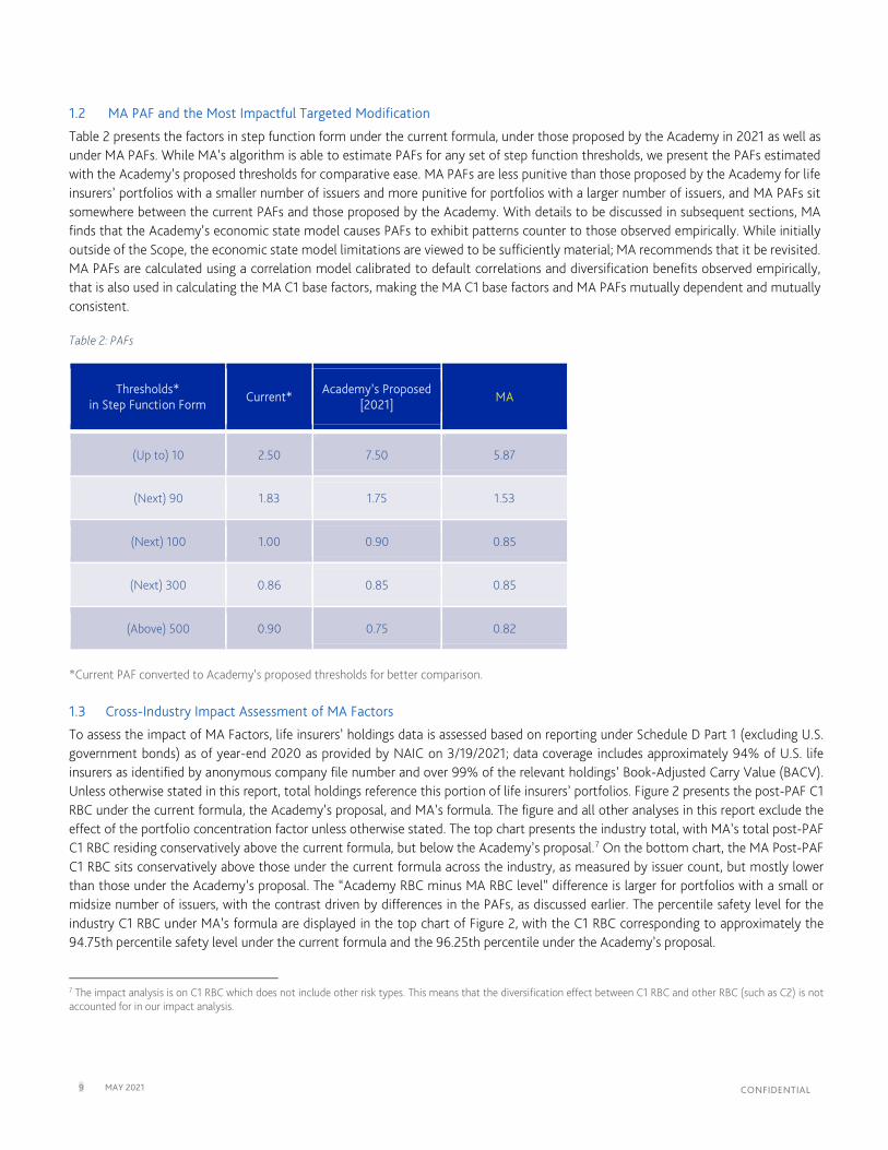
Table 2 presents the factors in step function form under the current formula, under those proposed by the Academy in 2021 as well as under MA PAFs. While MA’s algorithm is able to estimate PAFs for any set of step function thresholds, we present the PAFs estimated with the Academy’s proposed thresholds for comparative ease. MA PAFs are less punitive than those proposed by the Academy for life insurers’ portfolios with a smaller number of issuers and more punitive for portfolios with a larger number of issuers, and MA PAFs sit somewhere between the current PAFs and those proposed by the Academy. With details to be discussed in subsequent sections, MA finds that the Academy’s economic state model causes PAFs to exhibit patterns counter to those observed empirically. While initially outside of the Scope, the economic state model limitations are viewed to be sufficiently material; MA recommends that it be revisited. MA PAFs are calculated using a correlation model calibrated to default correlations and diversification benefits observed empirically, that is also used in calculating the MA C1 base factors, making the MA C1 base factors and MA PAFs mutually dependent and mutually consistent. Table 2: PAFs
Thresholds* in Step Function Form
Current* Academy’s Proposed
[2021] MA
(Up to) 10 2.50 7.50 5.87
(Next) 90 1.83 1.75 1.53
(Next) 100 1.00 0.90 0.85
(Next) 300 0.86 0.85 0.85
(Above) 500 0.90 0.75 0.82
*Current PAF converted to Academy’s proposed thresholds for better comparison.
1.3 Cross-Industry Impact Assessment of MA Factors
To assess the impact of MA Factors, life insurers’ holdings data is assessed based on reporting under Schedule D Part 1 (excluding U.S. government bonds) as of year-end 2020 as provided by NAIC on 3/19/2021; data coverage includes approximately 94% of U.S. life insurers as identified by anonymous company file number and over 99% of the relevant holdings’ Book-Adjusted Carry Value (BACV). Unless otherwise stated in this report, total holdings reference this portion of life insurers’ portfolios. Figure 2 presents the post-PAF C1 RBC under the current formula, the Academy’s proposal, and MA’s formula. The figure and all other analyses in this report exclude the effect of the portfolio concentration factor unless otherwise stated. The top chart presents the industry total, with MA’s total post-PAF C1 RBC residing conservatively above the current formula, but below the Academy’s proposal.7 On the bottom chart, the MA Post-PAF C1 RBC sits conservatively above those under the current formula across the industry, as measured by issuer count, but mostly lower than those under the Academy’s proposal. The “Academy RBC minus MA RBC level” difference is larger for portfolios with a small or midsize number of issuers, with the contrast driven by differences in the PAFs, as discussed earlier. The percentile safety level for the industry C1 RBC under MA’s formula are displayed in the top chart of Figure 2, with the C1 RBC corresponding to approximately the 94.75th percentile safety level under the current formula and the 96.25th percentile under the Academy’s proposal.
7 The impact analysis is on C1 RBC which does not include other risk types. This means that the diversification effect between C1 RBC and other RBC (such as C2) is not accounted for in our impact analysis.

10 MAY 2021 CONFIDENTIAL
Figure 2: Total Industry Post-PAF C1 RBC
Figure 3 takes a closer look at each portfolio’s Post-PAF C1 RBC under the MA and Academy proposals as a percentage of Post-PAF C1 RBC under the current formula. The RBC level, on the x-axis, is presented in log scale, to help visualize the impact across the entire industry. As discussed, MA’s proposal is conservative across the industry, as seen with most of the blue circles residing above 100% of the current RBC. The increase in RBC under the Academy’s proposal, represented by green triangles, is larger for portfolios with a lower current Post-PAF C1 RBC and is consistent with that observed in Figure 2. Outlying portfolios that experience large increases in RBC under the proposed formulas have few (generally fewer than 10) issuers, as circled in red, with the increase driven primarily by the proposed PAF rather than the proposed C1 base factors.
37.82
43.19 41.83
0
5
10
15
20
25
30
35
40
45
50Bi
llion
($)
Current Academy Proposal MA
~94.75 percentile safety levelunder MA Factors
~96.25 percentile safety levelunder MAFactors
96 percentile safety levelunder MAFactors
0
1
2
3
4
5
6
7
8
Billio
n ($
)
Issuer Count
Current Academy Proposal MA

11 MAY 2021 CONFIDENTIAL
Figure 3: Ratio of Life Company’s Post-PAF C1 RBC Proposed-to-Current Post-PAF C1 RBC
The remainder of this document is structured as follows: Section 2 provides a summary of MA’s proposed target modifications to the C1 factors, with an assessment of their impacts; Section 3 presents MA’s general understanding of the current RBC C1 formula and the Academy’s proposal; Section 4 presents a full exposition of the data and methodologies underpinning the proposed targeted modifications to the C1 factors, along with articulated limitations; Section 5 provides a comprehensive impact analysis; Section 6 provides sensitivity analysis for each of the targeted modifications; Section 7 outlines proposed next steps; and Section 8 presents a technical appendix.
2 Summary of MA’s Targeted Modifications to the C1 Factors
This section provides a summary of MA’s targeted modifications to the C1 factors presented in Table 3.
0%
100%
200%
300%
400%
500%
600%
0 1 10 100 1,000 10,000
Prop
osed
RB
C/C
urre
nt R
BC
Post-PAF RBC Under Current Formula (Million $; log scale)
Academy Proposal MA Current
Generally, portfolio with fewer than 10 issuers, sometimes a single

12 MAY 2021 CONFIDENTIAL
Table 3: Summary of MA’s Targeted Modifications to the C1 Factors
Targeted Modification
Current Academy-Proposed MA
Corrected possible errors in the engine code8
Limited documentation
Code that replicates Academy’s results suggests two possible errors: First, the four-state model used different simulation seeds for default rates and LGD economic state. Second, when removing the mean simulated portfolio loss, the model used the product of expected default rate and expected LGD, neglecting LGD and default correlation.
Corrected possible simulation engine errors (1) Default rates and LGD are drawn from the same economic state for Baa-Caa MIS rated issuers; and (2) Removed mean adjustment from simulated portfolio loss (Section 6.2.6 demonstrates limited concern for simulation noise).
Discount Rate & Tax Rate
Tax rate: 35% Discount rate: 9.23% (6% after tax) Recovery of tax loss benefit: 75% Tax recovery on default: 26.25%
Tax rate: 21% (2021) Discount rate (1993-2013 window): 5% (3.95% after tax) Recovery of tax loss benefit: 80% Tax recovery on default: 16.8%
Tax rate: 21% Discount rate (2000-2020 window): 3.47% (2.74% after tax) under guidance from the Life Risk-Based Capital (E) Working Group on April 22, 2021 Recovery of tax loss benefit: 80% Tax recovery on default: 16.8% While an alternative window start date can be justified, the discount rate enters the C1 formula as a single static rate and not as impactful as some other targeted modifications, reinforced by updated tax rate offset. Potentially important term structure dynamics that interplay with credit risk are not captured within the current framework.
Loss Given Default (LGD)
Limited documentation Average LGD by NAIC designation 37.25% (NAIC 1), 52.17% (NAIC 2), 56.67% (NAIC 3-5)
Does not align with the date of default. This deviation can result in bias with recovery rate levels, as well as their relationships with default rates. Average value of LGD = 53%
Use MA’s Default & Recovery Database (DRD) over 1987−2019 window, reflect the loss experience of life insurers’ U.S. corporate holdings across sectors, reflect issuer-level LGD to avoid overweighting outliers, align ultimate recovery with default date. Average value of LGD = 52%
Risk Premium Set equal to expected loss
Set equal to expected loss
Set at expected loss plus 0.5 standard deviation, recognizing variation in industry reserving standards and to closer align with reserving standards generally aimed at covering moderately adverse conditions and PBR. In addition, MA outlines a potential future update to AVR allowing alignment with default rates and LGDs that parameterize the final C1 framework; although this update is not urgent given AVR does not impact the RBC ratio and solvency. A higher Risk Premium lowers the C1 base factors and mildly increases their differentiation across the NAIC designation categories.
Economic State Model
Limited documentation Five-state model; affects both default and LGD; MA did not analyze, possibly similar properties to recent Academy proposal
A combination of two and four-state model; affects both default and LGD; Model results in C1 base factors that are not sufficiently differentiated across NAIC designation categories and under certain parameterizations C1 base factors that are not monotonic, and PAFs that provide more diversification benefits than observed empirically.
Initially outside Scope, economic state model limitations are viewed to be sufficiently material to warrant replacement by a correlation model that reflects default correlations and diversification benefits observed empirically in MA C1 Factors. Resulting C1 base factors are more differentiated across NAIC designation categories, and PAFs are a more accurate reflection of diversification benefits.
Default Rates
Based on data from, Moody’s 1991 Special Comment: Corporate Default and Recovery Rates, 1970-1990. Documentation on data treatment is limited
Smoothed corporate default rate term structures grouped by MIS alphanumeric rating using Academy’s algorithm.
Smoothed corporate default rate term structures representing the historical experience of life insurers’ U.S. corporate holdings using default data grouped by MIS alphanumeric rating using MA’s DRD. MA default rates tend to have a steeper slope (more differentiated across MIS ratings) than those proposed by the Academy, with differentiation more closely aligning with benchmarks.
PAFs Documentation is limited
Based on an economic state model that implies more benefits to diversification across issuers than observed empirically, resulting in a PAF that is overly punitive (lenient) to portfolios with a smaller (larger) number of issuers.
Initially outside Scope, economic state model limitations are viewed to be sufficiently material that the economic state model is replaced by a correlation model that reflects default correlations and diversification benefits observed empirically in MA C1 Factors. Resulting C1 base factors are more differentiated across NAIC designation categories, and PAFs are a more accurate reflection of diversification benefits.

13 MAY 2021 CONFIDENTIAL
The impact of each proposed targeted modification on the C1 base factors is presented in Table 4.
» The first four columns include the NAIC designation categories under the MIS rating scale, the current factors, and the Academy’s proposed factors.
» Column 5 presents MA’s replication of the 2017 Academy proposed factors, within the simulation noise of Column 4, ensuring the Academy’s data and methodologies are understood.
» Column 6 presents the replicated model, with possible errors in the Academy’s implementation of the simulation engine corrected, resulting in a mild reduction in the C1 factors.
» Column 7 incorporates the updated discount and tax rates results in a mild reduction in the C1 factors.
» Column 8 incorporates MA’s LGD distribution with a mean (52%) that is slightly lower than the Academy proposed (53%), resulting in a mild reduction in the factors.
» Column 9 presents the Risk Premium set at expected loss plus 0.5 standard deviation (previous columns set with the Academy’s proposed expected loss), with investment grade and high-yield MIS rating category C1 base factors reduced by approximately 20% and 15%, respectively, resulting in a mild increase in the overall C1 base factor slope.
» Column 10 replaces the economic state model with MA’s correlation model resulting in C1 base factors that are, in general, materially higher.
o Overall, the correlation model results in C1 base factors increasing by 24% on average for investment grade ratings and 28% on average for high-yield MIS ratings as depicted by the red rectangles.
o The counterfactual increases and decreases to the C1 base factors across the MIS ratings scale are highlighted in the orange and light blue rectangles.
Orange rectangles highlight Ba3 and B1 C1 base factors as an example of the economic state model resulting in more punitive C1 base factors for a higher MIS rating. The Academy’s 2021 proposed C1 base factor (column 3) for Ba3 (5.97%) is close to that for B1 (6.15%) as a result of the Ba3 Economic Scalars being more punitive relative to those for B1. Notice that under the column 9 parameterization, the Ba3 C1 base factor is larger than B1 C1 base factor (that is, the C1 base factors are counterintuitively non-monotonic). C1 base factor for Ba3 (5.995%) is substantially differentiated from that for B1 (7.854%) in column 10, as the more punitive contraction Economic Scalars no longer flatten the C1 base factors across Ba3 and B1 under the correlation model.
Light blue rectangles highlight A3 and Baa1 C1 base factors as an example of the economic state model resulting in more differentiation in C1 base factors for a higher MIS rating, with the increase along the MIS rating at 22% (column 9), compared with 11% under the MA correlation model (column 10).
» Column 11 presents MA’s base factors, utilizing MA’s default rates, which are generally lower and more differentiating across MIS ratings, particularly in the Aa3 to Baa3 range, than those used by the Academy. The larger differentiation in MA’s base factors due to the update in default rates is highlighted by green boxes in Columns 10 and 11, which shows that the ratio of the Baa3 factor to the Aa3 factor is 4.1 under MA’s base factors compared to 2.7 under MA’s base factors parametrized with the Academy’s default rate.
8 MA did not have access to the Academy’s model and stipulates these errors based on the following: we were not able to match the Academy’s proposed C1 base factors [2017] closely when relying only on the Academy’s documentation. Discussions with industry members lead us to find two errors, that when purposefully introduced, allowed for matching Academy’s proposed factors within simulation noise. First, the four-state model under the matched model used different simulation seeds for default rates and LGD economic state. Second, when removing the mean simulated portfolio loss, the matched model used the product of expected default rate and expected LGD, neglecting LGD and default correlation.

14 MAY 2021 CONFIDENTIAL
Table 4: Incremental Effects of Proposed Targeted Modifications on C1 Base Factors
(1) (2) (3) (4) (5) (6) (7) (8) (9) (10) (11)
MIS Rating9
Current C1 Base Factors
Academy's Proposed CA Base Factors
[2021]
Academy's Proposed C1 Base Factors
[2017]
MA's Replication
Under Academy
Parameters and Settings
[2017]
MA’s Replication Under Academy Parameters with
Corrected Simulation
Engine
(6) + MA’s Discount Rate
& Tax Rate (7) + MA’s LGD
(8) + Risk Premium at
mean + ½ SD
(9) + Economic
State Model Replaced with
Correlation Model
(10) + MA’s Default Rates [MA C1 Base
Factors]
Aaa 0.390% 0.290% 0.310% 0.319% 0.313% 0.322% 0.302% 0.254% 0.289% 0.158%
Aa1 0.390% 0.420% 0.430% 0.444% 0.444% 0.457% 0.440% 0.373% 0.412% 0.271%
Aa2 0.390% 0.550% 0.570% 0.602% 0.572% 0.589% 0.568% 0.476% 0.550% 0.419%
Aa3 0.390% 0.700% 0.720% 0.739% 0.722% 0.742% 0.711% 0.593% 0.715% 0.523%
A1 0.390% 0.840% 0.860% 0.901% 0.870% 0.892% 0.854% 0.694% 0.896% 0.657%
A2 0.390% 1.020% 1.060% 1.044% 1.001% 1.026% 1.004% 0.817% 1.046% 0.816%
A3 0.390% 1.190% 1.240% 1.194% 1.161% 1.193% 1.151% 0.921% 1.254% 1.016%
Baa1 1.260% 1.370% 1.420% 1.445% 1.410% 1.449% 1.394% 1.128% 1.388% 1.261%
Baa2 1.260% 1.630% 1.690% 1.710% 1.593% 1.636% 1.611% 1.287% 1.633% 1.523%
Baa3 1.260% 1.940% 2.000% 2.017% 1.910% 1.972% 1.933% 1.542% 1.956% 2.168%
Ba1 4.460% 3.650% 3.750% 3.716% 3.475% 3.558% 3.397% 2.848% 3.955% 3.151%
Ba2 4.460% 4.660% 4.760% 4.710% 4.393% 4.501% 4.470% 3.739% 4.840% 4.537%
Ba3 4.460%
5.970% 6.160% 6.258% 5.744% 5.859% 5.895% 4.952% 5.995% 6.017%
B1 9.700% 6.150% 6.350% 6.287% 5.909% 6.039% 6.018% 4.920% 7.854% 7.386%
B2 9. 700% 8.320% 8.540% 8.544% 7.814% 7.977% 7.937% 6.614% 9.901% 9.535%
B3 9.700% 11.480% 11.820% 11.461% 10.739% 10.971% 10.988% 9.319% 12.679% 12.428%
Caa1 22.310% 16.830% 17.310% 16.563% 14.932% 15.206% 15.364% 13.364% 16.044% 16.942%
Caa2 22.310% 22.800% 23.220% 22.637% 20.283% 20.626% 20.826% 18.788% 19.870% 23.798%
Caa3 22.310% 33.860% 34.110% 34.046% 32.431% 32.673% 32.494% 31.359% 28.933% 32.975%
9 NAIC designation categories presented under MIS rating scale. NAIC designation categories presented under MIS rating scale
4.1X 2.7X
24%
28%

15 MAY 2021 CONFIDENTIAL
3 Current RBC C1 Formula and Academy’s Proposal
The NAIC RBC formulas are for the purpose of identifying potentially weakly capitalized insurance companies. RBC establishes a de facto minimum amount of capital to be held by insurers in order to avoid regulatory intervention. This minimum capital amount protects statutory surplus from the fluctuations that reduce statutory surplus, including credit risk, deferral risk, subordination risk, and event risk (American Academy of Actuaries, 2015). C1 capital provides protection from statutory insolvency due to losses in statutory asset value resulting from bond defaults, common stock depreciation, and other changes associated with investment flowing through statutory surplus. The prevailing C1 factors were implemented and reported in 1994, with reference to 1970−1990 default experiences. The C1 Factor Proposal by the Academy was revised multiple times during the 2015−2021 period in response to stakeholder feedback. While the proposed C1 factors were developed based on the loss experience of public U.S. corporate bonds, the same set of factors are recommended for all fixed income securities in NAIC’s Schedule D, which is used to report long-term bonds and stocks owned, acquired, sold, redeemed, or otherwise disposed of by insurers during a year. RMBS/CMBS securities are generally filed with NAIC Securities Valuation Office (SVO) and assigned NAIC designations through a financial modeling process conducted by the NAIC Structured Securities Group (SSG), subject to limited filing exemptions (NAIC Securities Valuation Office and NAIC Structured Securities Group, 2019). C1 factors are applied to RMBS/CMBS securities based on the NAIC designations. Based on discussions with the ACLI, other structured securities are treated identically as bonds and are not required to go through the NAIC designation process. C1 capital is intended to cover the 96th percentile portfolio loss in excess of those anticipated in statutory reserves over a 10-year horizon. The portion of default loss already anticipated in statutory reserves is reflected in the capital fund as Risk Premium, which is modeled as the annual mean loss from default (after tax and considering recoverable tax on default loss) derived from baseline default and recovery rate assumptions. Risk Premiums are assumed to earn 5% pre-tax interest per annum. Key inputs to the framework are as follows:
» Baseline default rates are estimated using 1983−2012 default data, sourced from (Moody's Investors Service, 2013) as referenced in (American Academy of Actuaries, 2015). For each MIS rating, the marginal default rates in Years 1 through 10 are smoothed using a 4th-degree polynomial regression to remove noise. Default rates are differentiated across economic states (for example, expansion or contraction) using a set of estimated scalars (Economic Scalars).
» Baseline recovery rates are estimated using recovery data of senior unsecured bonds provided by Standard & Poor’s, covering 1987−2012.
» Representative portfolios for the seven categories are constructed based on life insurers' holdings provided by NAIC to the Academy. The final representative portfolio size is set as $10 to $25 billion. Issuers’ holding amounts are estimated from a sample of actual life insurers’ portfolios (American Academy of Actuaries, 2015). Only the holding amounts of NAIC-1 and NAIC-2 issuers (824 total) in this portfolio are used to determine the holding amount for each bond in the portfolio, for every MIS rating category in the simulation model. In other words, the representative portfolio for each MIS rating category only differs by issuer MIS rating.
With key inputs in hand, the C1 base factor for each MIS rating category is calculated separately through a simulation model. It represents the amount of initial funds needed to cover the 96th percentile greatest default loss over 10 years, offset by the portion of default loss already anticipated in statutory reserves, proxied through each MIS rating’s Risk Premium. The modeling framework relies on the following calculation steps:
» Simulate annual economic state for 10 years and identify the corresponding Economic Scalar in each year.
» The default rate for each MIS rating category in each year is determined by multiplying the baseline default rate term structure by the Economic Scalar from the previous step.
» Defaults across issuers are simulated under the scaled default rate.
» The simulated economic state from step 1 determines the distribution of LGD that is simulated for each defaulted issuer.
» The maximum 10-year cumulative portfolio loss, which considers recoverable tax on default loss and accumulated Risk Premium offsets, is calculated over each of the 10-year, representative aggregated portfolio loss; offsets may result in the maximum loss being realized prior to year 10.
» Set the base C1 factor for each MIS rating category as the initial fund required to cover the maximum loss at 96th percentile safety level.

16 MAY 2021 CONFIDENTIAL
These C1 base factors (Table 1) and life insurers’ holdings determine Pre-PAF C1 RBC. The PAF (Table 2) is determined by the number of issuers and applied to the entire portfolio to arrive at the Post-PAF C1 RBC. An additional concentration factor (doubling of top-ten holdings) is applied and discussed in Section 8.4. The next section presents data and methodology details related to each of the MA targeted modifications to the C1 factors. 4 Targeted Modifications: Data, Methodology, and Limitations
This section provides data and methodology details underpinning the MA targeted modifications to the C1 base factors and PAFs, along with articulated limitations. Section 4.1 describes the range of discount rates explored and updated tax rate; Section 4.2 reviews modifications to the LGD distribution; Section 4.3 updates the Risk Premium; Section 4.4 updates default rates to more closely reflect the historical experience of life insurers’ holdings; Section 4.5 revisits the economic state model and introduces the MA correlation-based model; Section 4.6 explores bounds on base factors to align with factors and treatment of other asset classes; Section 4.7 updates the PAF to align with concentration losses observed empirically.
4.1 Explored Range of Discount Rates Based on Several Time Windows and Updated Tax Rate
4.1.1 Summary of MA’s Update
MA‘s updates the tax rate to 21%, reflecting the 2017 Tax Reconciliation Act, as well as the discount rate estimation window to cover 2000-2020 (from 1993-2013), resulting in a discount rate of 3.47% (from 5%) under guidance from the Life Risk-Based Capital (E) Working Group on April 22, 2021. 4.1.2 MA’s Update
In the C1 model, the after-tax discount rate is used as the discount factor to calculate the net present value of projected cash flows and to serve as the risk-free rate earned on Risk Premium, to be discussed later. To more closely reflect the current, and expected, interest rate environment, MA uses the updated 2000-2020 window to estimate the discount rate; the Academy’s window covers 1993-2013. In addition, the effect of the 2017 Tax Reconciliation Act is incorporated, in which the U.S. corporate tax rate was lowered from 35% to 21%; as does the Academy in its most recent 2021 update (American Academy of Actuaries, 2021). The resulting tax recovery on default changes from 28% to 16.8%, maintaining the assumption of an 80% recovery of capital loss tax benefit used by the Academy. In comparison, the Academy’s model sets the Discount Rate at 5.02% pre-tax (further rounded to 5%), the average 10-year LIBOR swap rate from 1993-2013. However, the exact source is not referenced, and the time-series data is not made available to MA. Rather, the 10-year USD swap rate from the Federal Reserve H.15 Daily Selected Interest Rates Release and Intercontinental Exchange (ICE) serves as a proxy in our analysis.10 Figure 4: shows the downward trend in the 10-year USD swap rate over the most recent two decades. The rate is below 3% for most of the 2011-2021 period. Since the Federal Reserve took extensive measures to support the economy during the global pandemic (Federal Reserve, 2020), the rate decreased further, under 1% at times.11
10 ICE data was used starting August 1, 2014.
11 The November Minutes of the Federal Open Market Committee quotes, “The Committee decided to keep the target range for the federal funds rate at 0−¼% and expects it will be appropriate to maintain this target range until labor market conditions have reached levels consistent with the Committee’s assessments of maximum employment and inflation has risen to 2% and is on track to moderately exceed 2% for some time” (the Federal Open Market Committee, 2020).

17 MAY 2021 CONFIDENTIAL
Figure 4: 10-Year USD Swap Rate
Source: Federal Reserve System H.15 Daily Selected Interest Rate (July 3, 2000−July 31, 2014) and Intercontinental Exchange
(data on or after August 1, 2014).
.
MA recognizes the need to parameterize the discount rate with a long-term perspective of interest rates, and the desire for this parameter to be relatively stable, while also allowing a closer reflection of the current, low-rate, environment. Several possible candidate windows were considered for computing discount rates. The pre-tax discount rate entering MA’s C1 Factors is 3.47%, the average of daily 10-year USD swap rate in 2000-2020 under guidance from the Life Risk-Based Capital (E) Working Group on April 22, 2021. MA’s after-tax discount rate will be 2.74%, lower than the Academy’s 3.25% in the 2017 proposal and 3.95% in the 2021 proposal in which the Academy updated the tax rate to 21% and kept the pre-tax discount rate unchanged (American Academy of Actuaries, 2021).
Using MA’s pre-tax discount rate (3.47) and tax rate (21%), C1 base factors increase slightly as seen in Figure 21 in Section 6.1. Two alternative time windows for pre-tax discount rates have been considered, 1993-202012 (4.32%) and 2010-2020 (2.25%). Sensitivity of the C1 base factors to these time windows is reported in Section 6.2.1. Using 2000-2020 (3.47%) as the point of reference, the 1993-2020 (4.32%) and 2010-2020 (2.25%) windows result in a mild decrease and increase in C1 base factors respectively; lower discount rate leads to higher C1 base factors as the present values of future losses are higher. Section 6.2.1 discusses the details.
The discount rate enters the C1 formula as a single static rate. Potentially important term structure dynamics that can interplay with credit risk are not captured within the current framework. In addition, the chosen rate is calculated based on historical data and may not necessarily prevail in the future. With these limitations in mind:
» MA C1 Factors are parametrized with a discount rate based on the 2000−2020 window (3.47%) under guidance from the Life Risk-Based Capital (E) Working Group on April 22, 2021
» MA recommends revising the framework to consider the term-structure dynamics and its heterogeneous impact across asset classes that have varying timing of cash flows13
12 The discount rate for 1993-2020 is calculated as the average of the Academy’s discount rate computed from 1993–2013 (5.02%) and the Federal Reserve and Intercontinental Exchange (ICE) USD swap rates from 2014–2020, weighted by the number of business days. 13 See references in (Moody's Analytics, 2021) which highlights cases where interest income plays a material role in the risk profile of a credit security.
0
1
2
3
4
5
6
7
1/2/2001 1/2/2006 1/2/2011 1/2/2016 1/2/2021
(in %
)

18 MAY 2021 CONFIDENTIAL
4.2 Updated LGD Distribution to More Closely Align with Empirical Patterns
4.2.1 Summary of MA’s Update
MA’s LGD distribution is updated:
» Using MA’s DRD over the 1987−2019 window
» To reflect the historical loss experience of life insurers’ U.S. corporate holdings across sectors
» To reflect issuer-level LGD to avoid overweighting outliers
» To choose the data source of ultimate recovery for each default based on MIS recommendation reported in the DRD (e.g., the data sources of ultimate recovery calculation are settlement, liquidity or trading price)
MA’s LGD distribution has a mean of 52% that is slightly lower than the 53% proposed by the Academy. For comparison, the current RBC framework includes LGD distributions that differ by NAIC designations (NAIC 1-5), with average LGD 37.25% (NAIC 1), 52.17% (NAIC 2) and 56.67% (NAIC 3-5) (American Academy of Actuaries, 2015). 4.2.2 MA’s Update
This section describes the steps taken by the Academy to estimate LGD distributions and MA’s. We begin with a brief description of the Academy’s model and approach to estimating LGD-related parameters. We then discuss the data, methodologies and limitations associated with our targeted modifications that build off the Academy’s approach. The C1 factors proposed by the Academy employ two empirical distributions for LGD, corresponding to economic contractions and expansions that underlie the economic state model. These distributions are nonparametric, estimated and used in the model as follows (American Academy of Actuaries, 2015):
1. LGD distribution is estimated using ultimate recovery data of senior unsecured bonds provided by Standard & Poor’s, covering 1987-2012
2. Bond-level LGD data is grouped into contraction and expansion periods and placed into 11 buckets, <0, 0-10%, 10-20%, etc., each bucket associated with an average LGD and historical probability of occurrence for the LGD observations. Negative LGD corresponds to recovery greater than par value
3. The relative frequencies of historical LGD are used as the probability of occurrence for each bucket. For each trial, LGD is simulated from the bucketed probability distribution, where a bucket is selected first and then the average LGD of the selected bucket is used
MA maintained the same basic elements of the Academy’s LGD modeling framework, but incorporated several changes so that the LGD estimates more closely align with the historical loss experience of life insurers’ holdings:
» The time window for LGD estimation is expanded to 1987-2019 from 1987-2012. MA excluded the data from 2020 for two reasons: (1) Some bonds may still be in early stages of recovery due to the lengthy workout process; and (2) at the time of this estimation the NBER had not yet classified the economic state of 2020. MA’s LGD was assessed to ensure comparability with underlying data used by the Academy. The average LGD of senior unsecured bonds in 1987-2012 using MA’s DRD is 52.9% with 1,261 bond defaults.
» MA estimates bond LGDs using MIS recommended recovery data source for each default, as reported in the DRD (e.g., settlement, liquidity or trading price).
» MA uses issuer-level LGD instead of bond-level LGD to limit outsize influence of issuers that had many bonds outstanding at the time of default. The issuer-level LGD is defined as the principal-weighted average of LGDs for all bonds of the same issuer in a default event. For example, 49 senior unsecured bonds from Pacific Gas & Electric (PG&E) defaulted, all with zero LGD in 2001, one of the four contraction years. PG&E bonds accounted for 25% of defaulted bonds in 2001. For 2001, the average bond-level LGD is 56%, while the average issuer-level LGD is 78%. The estimated LGD distribution for economic contraction will, therefore, be influenced heavily by PG&E bond defaults. We group issuer-level LGD data into expansion years and contraction years by the year of default rather than the year of emergence. This step ensures consistency with the simulation engine, where loss is calculated at the time of default.

19 MAY 2021 CONFIDENTIAL
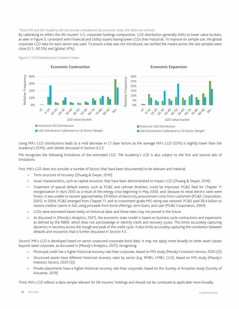
» We weight the frequency of LGD observations to reflect life insurers’ year-end 2020 U.S. corporate holdings across the Industrial, Financial, and Utility sectors as discussed in Section 5.1. Notice the variation in LGD across sectors, with the Utility sector averaging a low 17%, in contrast to the Industrial sector at 62%. The historical LGD observations are heavily concentrated in Industrial, outweighing the proportion of Industrial exposures in the life insurers’ holdings. We calibrate the empirical LGD distribution to reflect the sector composition of life insurers’ U.S. corporate holdings. The following steps are taken:
- Segregate the historical issuer LGD observations by economic expansion and contraction years
- For each economic state, expand the sample by scaling the frequency of the underweighted sectors (Financial and Utility) to match the holdings weight
- The size of the expanded sample (𝑛𝑛𝑒𝑒𝑒𝑒𝑒𝑒𝑒𝑒𝑒𝑒𝑒𝑒𝑒𝑒𝑒𝑒) is scaled by the ratio of dividing the number of LGD observations for the Industrial sector (𝑛𝑛𝑖𝑖 ) by its holdings weight (ℎ𝑤𝑤𝑖𝑖). This step ensures that the LGD observations for Industrial remain unchanged in the expanded sample.
o The number of observations for Financial and Utility in the expanded sample will be 𝑛𝑛𝑒𝑒𝑒𝑒𝑒𝑒𝑒𝑒𝑒𝑒𝑒𝑒𝑒𝑒𝑒𝑒 × ℎ𝑤𝑤𝑓𝑓 and 𝑛𝑛𝑒𝑒𝑒𝑒𝑒𝑒𝑒𝑒𝑒𝑒𝑒𝑒𝑒𝑒𝑒𝑒 × ℎ𝑤𝑤𝑢𝑢 respectively
o Then the LGD observations in the original sample for Financial and Utility will be replicated 𝑒𝑒𝑒𝑒𝑒𝑒𝑒𝑒𝑒𝑒𝑒𝑒𝑒𝑒𝑒𝑒𝑒𝑒 × ℎ𝑤𝑤𝑓𝑓
𝑒𝑒𝑓𝑓
and 𝑒𝑒𝑒𝑒𝑒𝑒𝑒𝑒𝑒𝑒𝑒𝑒𝑒𝑒𝑒𝑒𝑒𝑒 × ℎ𝑤𝑤𝑢𝑢
𝑒𝑒𝑢𝑢 times, respectively
» Aggregate issuer-level LGD for each economic state group into buckets of <0%, 0-10% … up to 90%-100%. The empirical LGD distribution consists of the average LGD of each bucket with the probability being the proportion of observations.
We now shift our attention to data and parameterization. Section 5.1 discusses the differences in sector composition of life insurers’ U.S. corporate holdings and issuance, recognizing potential drivers such as insurers’ appetite for medium- and long-term assets in asset-liability matching considerations (The NAIC Capital Markets Bureau, 2021). To more closely reflect the loss experience of life insurers’ corporate holdings, life insurers’ sector holdings detailed in Table 16 of Section 5.1 is used in conjunction with sector LGD data detailed in Table 5.
LGDs for senior unsecured bonds are shown by study period, source, and economic state grouping in Table 6. The difference between the MIS and the Academy is primarily driven by MIS averaging across issuers, while the Academy averages across issues. The differences between the MA and MIS values are primarily driven by MA sector weighting LGD. Table 5: Historical LGD Data in MA’s DRD (1987−2019)
Sector Contraction
Average Issuer-level LGD Expansion
Average Issuer-level LGD
Financial 31.6% 42.4%
Industrial 67.4% 59.6%
Utility 0.0% 34.1%
Table 6: Average LGD for Senior Unsecured Bonds
Period LGD Source for senior
unsecured bonds LGD for economic expansion years
LGD for economic contraction years
LGD for all years
1987−2019 MA estimated issuer- and U.S. life insurers’ holdings-sector weighted
50.3% 52.4% 52%
1983−2020 MIS issuer weighted overall sample average*
- - 62%
1987−2012 The Academy issue weighted* - - 53%
20 MAY 2021 CONFIDENTIAL
*Since MIS and the Academy did not provide a breakdown by economic state, the fields are omitted. By calibrating to reflect the life insurers’ U.S. corporate holdings composition, LGD distribution generally shifts to lower value buckets, as seen in Figure 5, consistent with Financial and Utility issuers having lower LGDs than Industrial. To improve on sample size, the global corporate LGD data for each sector was used. To ensure a bias was not introduced, we verified the means across the two samples were close (U.S.: 60.5%) and (global: 61%). Figure 5: LGD Distribution for Economic States
Using MA’s LGD distributions leads to a mild decrease in C1 base factors as the average MA’s LGD (52%) is slightly lower than the Academy’s (53%), with details discussed in Section 6.2.2.
MA recognizes the following limitations of the estimated LGD. The Academy’s LGD is also subject to the first and second sets of limitations.
First, MA’s LGD does not consider a number of factors that have been documented to be relevant and material:
» Term-structure of recovery (Zhuang & Dwyer, 2016)
» Issuer characteristics, such as capital structure, that have been demonstrated to impact LGD (Zhuang & Dwyer, 2016)
» Treatment of special default events, such as PG&E and Lehman Brothers, could be improved. PG&E filed for Chapter 11 reorganization in April 2001 as a result of the energy crisis beginning in May 2000, and, because its retail electric rates were frozen, it was unable to recover approximately $9 billion of electricity procurement costs from customers (PG&E Corporation, 2001). In 2004, PG&E emerged from Chapter 11, and its investment-grade MIS rating was restored. PG&E paid $8.4 billion to resolve creditor claims in full, using proceeds from bond offerings, term loans, and cash (PG&E Corporation, 2004)
» LGDs were estimated based solely on historical data, and those rates may not prevail in the future
» As discussed in (Moody's Analytics, 2021), the economic state model is based on business cycle contractions and expansions as defined by the NBER, which does not acknowledge or identify credit and recovery cycles. This limits accurately capturing dynamics in recovery across the trough and peak of the credit cycle. It also limits accurately capturing the correlation between defaults and recoveries that is further discussed in Section 4.5
Second, MA’s LGD is developed based on senior unsecured corporate bond data. It may not apply more broadly to other asset classes beyond rated corporate, as discussed in (Moody's Analytics, 2021), recognizing:
» Municipal credit has a higher historical recovery rate than corporate, based on MIS study (Moody's Investors Service, 2020 (2))
» Structured assets have different historical recovery rates by sector (e.g. RMBS, CMBS, CLO), based on MIS study (Moody's Investors Service, 2020 (3))
» Private placements have a higher historical recovery rate than corporate, based on the Society of Actuaries study (Society of Actuaries, 2019)
Third, MA’s LGD reflects a data sample relevant for life insurers’ holdings and should not be construed as applicable more broadly:
0%
10%
20%
30%
40%
Rela
tive
Freq
uenc
y
LGD value bucket
Economic Contraction
Historical LGD DistributionLGD Distribution Calibrated to US Sector Weight
0%5%
10%15%20%25%30%
Rela
tive
Freq
uenc
yLGD value bucket
Economic Expansion
Historical LGD DistributionLGD Distribution Calibrated to US Sector Weight
21 MAY 2021 CONFIDENTIAL
» The sector composition of life insurers’ holdings will change over time, and the relevance of the weighting should be evaluated accordingly
» A sector that is over-weighted in life insurers’ holdings relative to the rated universe may result in recovery rates that are overly impacted by that sector’s historical recovery rate
» The sectors’ historical LGD may not be indicative of future LGD
Recognizing these limitations MA’s C1 Factors are parametrized with MA’s LGD distribution, and MA recommends revisiting the framework to address the first and second set of limitations described above.
4.3 Risk Premium to More Closely Align with PBR and Industry Reserving Standards
4.3.1 Overview of MA’s Update
C1 RBC is the minimum required capital above statutory reserves buffering against a tail loss credit scenario. Statutory reserves are liabilities ensuring policy claims can be paid off under moderately adverse conditions. Risk Premium acts as an offset to RBC; it is the part of statutory reserves provisioned against default loss. In the C1 RBC model, its value is pre-determined according to the initial MIS rating of each issuer and is assumed to be evenly released annually in the simulation. A higher Risk Premium decreases C1 base factors and mildly increases differentiation (i.e., resulting steeper slope) across NAIC designation categories. Under VM-20 and VM-21, reserving is set to cover CTE 70 default loss. But VM-20 is only applicable to new life products. The in-force life products follow industry reserving standards that are commonly understood to aim at covering moderately adverse conditions. With variation in industry reserving standards, MA C1 Factors are parametrized with a Risk Premium at expected loss plus 0.5 standard deviation. A transition to expected loss plus one standard deviation should be considered as VM-20 becomes more widely applicable, and VM-22 is formally updated and widely applicable. 4.3.2 MA’s Update
By way of background, VM-20 and VM-21 are requirements for principle-based reserves (PBR) for Life Products and Variable Annuities. VM-20 stipulates that the statutory reserves should be calculated as the maximum of the Net Premium Reserve (NPR), Deterministic Reserve (DR), and Stochastic Reserve (SR). The calculations of statutory reserves under the DR and the SR are similar in spirit to the calculation of C1 RBC. In particular, DR and SR cover future policy claims, expenses, etc. while accounting for future cashflows including the insurance premium and investment income. Under VM-20 DR and SR, investment returns are calculated net of CTE 70 default losses (i.e., the Baseline Default Cost Factor) in the asset model. In this context, CTE 70 represents the mean between 70th and 100th percentiles of losses, which is approximated by the 88th percentile. This means that the statutory reserves under PBR already cover default loss up to the 88th percentile, which implies C1 RBC only needs to cover default loss in excess of the 88th percentile. In addition, VM-21, which applies to all in force, mandates that the Variable Annuity asset model also reflects the default cost prescribed by VM-20.14 VM-22 is also being updated so that the asset model for new Payout Annuities incorporates the same default cost. These rules suggest that setting Risk Premium at expected loss is too conservative. Instead, it would be appropriate to set Risk Premium at 88th percentile, or roughly expected value plus one standard deviation of default loss. However, VM-20 has only been applicable to new life products starting from 2017. This means that most life products on the books today are reserved according to the Commissioners Reserve Valuation Method (CRVM) and Commissioners Annuity Reserve Valuation Method (CARVM), which do not explicitly prescribe the level of default loss covered. Nevertheless, the coverage of VM-20 is increasing for new bond issuance. In addition, it is commonly understood that life companies set reserves conservatively, aiming to cover moderately adverse conditions. MA acknowledges that variation in industry reserving standards is a limitation to modeling the Risk Premium and parametrizes the conservative Risk Premium at expected loss plus 0.5 standard deviation. A transition to expected loss plus one standard deviation should be considered as VM-20 becomes more widely applicable, and VM-22 is formally updated and widely applicable.
14 While Variable Annuities in the general account is relatively small, all Variable Annuity’s statutory reserves go into the general account, increasing the materiality of the resulting offset to capital.

22 MAY 2021 CONFIDENTIAL
MA understands the Academy’s concern on the modification of Risk Premium as, “changing the [Risk Premium] would necessitate a review of statutory policy reserves, the default portion of the [Asset Valuation Reserve (AVR)] calculation and the treatment of AVR in the life risk-based capital (LRBC) ratio calculation” (American Academy of Actuaries, 2018). However, as pointed out by ACLI (American Council of Life Insurers, 2018),“under the statutory reserve framework, AVR is…an allocation of surplus, a somewhat arbitrary apportionment of assets to smooth the cyclicality of asset defaults; it is not a quantification of risk. This view is supported by the fact that the RBC formula includes AVR in available capital (i.e., an allocation of surplus) but excludes AVR from required capital (i.e., [it is] not a risk buffer). Consequently, addressing double-counting within the risk premium will not weaken policyholder protections below the intended levels.” These points raised by ACLI are represented in the RBC ratio formula depicted in Figure 6, where the allocation of surplus across AVR and unassigned surplus can be seen to not impact the RBC ratio. Figure 6: Allocation of Surplus Across AVR and Unassigned Surplus
While alignment between C1 RBC and AVR can be desirable, potential misalignment is not relevant for solvency or the RBC framework; the RBC framework is to help “identify potentially weakly capitalized companies”. In addition, we observe that MA proposed Risk Premium of expected loss plus 0.5 standard deviation (and expected loss + 1 standard deviation) generally sits close to or between the AVR basic contribution of expected loss and the AVR reserve objective factor of 85thpercentile of loss, which appears more aligned with the AVR requirement than setting Risk Premium as expected loss. To summarize, higher Risk Premium reduces the C1 base factors and mildly increases differentiation (i.e., resulting steeper slope) across MIS ratings. MA acknowledges that variation in industry reserving standards is a limitation to modeling the Risk Premium. MA C1 Factors are therefore parameterized with a conservative Risk Premium set at expected loss plus 0.5 standard deviation. A potential transition to expected loss plus one standard deviation should be considered, as VM-20 becomes more widely applicable, and VM-22 is formally updated and widely applicable.15 In addition, a future update to AVR allowing alignment with default rates and LGDs that parametrize the final C1 framework should be considered, although this update does not appear urgent given AVR does not impact the RBC ratio and solvency. As part of the sensitivity analysis, Section 6 reports C1 base factors under Risk Premium set at expected loss and expected loss plus one standard deviation. It can be seen that the value of C1 base factors varies materially under different levels of Risk Premium, highlighting the importance of this assumption. The C1 RBC is over 20% higher when the Risk Premium is set as expected loss plus 0.5 standard deviation instead of expected loss plus one standard deviation, confirming the conservatism built into the MA’s Risk Premium.
15 Separately, C3-Phase 1, which will be applicable to all in force Fixed an Indexed Annuities, will very likely require a similar default cost, at which point there will be a double counting of buffer for default loss between C1 and C3.
23 MAY 2021 CONFIDENTIAL
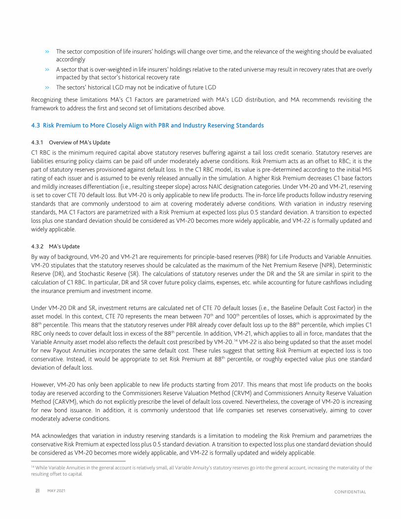
A final nuance worth noting is that the shape of the loss distribution varies across MIS ratings and can be seen from Table 7 where the percentile loss for expected loss, expected loss plus 0.5 standard deviation, and expected loss plus one standard deviation are presented. These percentiles are the ones used in MA’s factors. Table 7: Implied Loss Percentiles and Risk Premium Under MA’s Correlation Model
Expected Loss Expected Loss + 0.5 Standard Deviation Expected Loss + 1 Standard Deviation
MIS Rating16 Value Loss Percentile Value Loss Percentile Value Loss Percentile
Aaa 0.003% 75.0% 0.007% 83.7% 0.011% 89.7%
Aa1 0.008% 66.4% 0.015% 79.9% 0.021% 87.5%
Aa2 0.022% 61.4% 0.032% 76.0% 0.042% 85.8%
Aa3 0.032% 59.2% 0.046% 75.2% 0.059% 85.7%
A1 0.048% 58.5% 0.065% 74.8% 0.082% 85.3%
A2 0.070% 57.5% 0.092% 74.0% 0.113% 85.0%
A3 0.096% 57.2% 0.123% 74.4% 0.150% 85.5%
Baa1 0.134% 56.7% 0.168% 73.4% 0.202% 85.4%
Baa2 0.187% 55.1% 0.229% 73.1% 0.271% 85.1%
Baa3 0.303% 55.4% 0.362% 73.3% 0.421% 84.7%
Ba1 0.493% 55.0% 0.579% 72.6% 0.665% 84.8%
Ba2 0.809% 54.0% 0.932% 71.8% 1.055% 84.8%
Ba3 1.071% 54.5% 1.225% 72.4% 1.379% 84.7%
B1 1.429% 53.9% 1.619% 72.2% 1.809% 84.7%
B2 1.933% 53.2% 2.168% 71.5% 2.404% 84.7%
B3 2.545% 52.9% 2.834% 71.4% 3.123% 84.9%
Caa1 3.424% 53.0% 3.787% 71.3% 4.151% 84.1%
Caa2 4.816% 52.4% 5.274% 70.8% 5.731% 84.1%
Caa3 7.406% 51.9% 7.998% 70.2% 8.591% 83.9%
4.4 Baseline Default Rates to More Closely Align with Historical Experience of Life Insurers’ Corporate Holdings
4.4.1 Summary of MA’s Update
This section discusses MA’s approach to estimating default rate term structures representing the historical experience of life insurers’ corporate holdings using default data grouped by MIS alphanumeric rating. Recognizing challenges with empirical default rates, the section outlines the steps taken to mitigate data paucity and introduce both monotonicity and smoothness to the default rates using MA’s DRD and several benchmarks. MA’s default rates tend to have a steeper slope (more differentiated across MIS ratings) than those proposed by the Academy. The resulting default rates face articulated limitations, most prominently that MIS corporate ratings do not target specific default rates, and the assignment of any single set of default rate term structures to MIS ratings must depend on assumptions about stability and homogeneity that are not the basis of MIS rating assignments.
16 NAIC designation categories under MIS rating scale.

24 MAY 2021 CONFIDENTIAL
4.4.2 MA’s Update
This section describes how MA derived the default rate term structures for each MIS corporate rating and discusses limitations of interpretation and applicability. The underlying data that MA used is accessible through public sources, and methodologies are accessible and repeatable to the NAIC and industry on an ongoing basis.17 As discussed in the Executive Summary, the performance criteria required from default rates is their alignment with economic risks that reflect the historical experience of life insurers’ holdings. More specifically, we are looking for default rates that, when used in parameterizing the C1 factors, align insolvency risks with capital requirements across MIS rating categories for better identification of weakly capitalized firms; the C1 factors should not incentivize poor business decisions that can adversely impact solvency. The performance criteria are heuristic, given the inherent challenge of the RBC framework and the limitations to scope. Specifically, C1 factors are:
» Cardinal, and a function of MA‘s default rates estimated using Moody’s Investors Services corporate default rates that reflect the historical experience of life insurance corporate holdings for each MIS rating, which are opinions of ordinal, horizon-free credit risk, rather than cardinal
» Applied to a range of credit assets based on their NAIC designations, with statistical properties that can be different from those estimated using Moody’s Investors Services corporate default rates
MA does not assert that the default rate term structures, which were estimated based solely on historical data, will prevail in the future. The estimated default rate term structures have been developed solely in support of the purpose of the NAIC’s goal of setting C1 Bond Factors. With these challenges in mind, the MA default rate term structures, along with MA C1 Factors, are provided to the NAIC to use in setting the final RBC C1 factors.
With these considerations we explore the possible data sources and benchmarks that can be used when estimating default rates that are worth reviewing:
» Empirical corporate default rate term structure studies such as (Moody's Investors Service, 2021), that report corporate default rates by MIS ratings over a number of windows. While useful, the default rates are not appropriate in raw form within this context. While a broad review of the various published default rate term structures across the samples demonstrates general monotonic behavior, a close inspection shows instances of non-monotonicity in default rates that will flow into non-monotonicity in capital along the MIS ratings scale. For example, Table 9 which reproduces 10-year default rates from Exhibit 42, 43 and 44 in (Moody's Investors Service, 2021), exhibits instances of non-monotonicity. Column 3 – corresponding to Exhibit 43 of (Moody's Investors Service, 2021) – shows that default rates decrease from 2.339% to 2.211% and 2.2611%, respectively, across MIS alphanumeric ratings A2, A3 and Baa1. Similar instances can be observed for MA empirically estimated default rates in Table 8, Utility column, where default rates decrease between MIS ratings A and Ba from 1.745% to 1.098% and again between MIS ratings Caa to Ca from 19.364% to 16.130%. These findings reflect data sparsity and generally motivate the need to apply expert judgment, engage in data aggregation, interpolation, and smoothing to resolve noise. Separately, at the upper end of the credit spectrum, a dearth of defaults and possibly high average recovery makes historical default events difficult to use in isolation. For illustration, there have been six defaults within 10 years of being assigned an Aaa MIS rating from 1970 (with all defaults occurring after 1983). Similarly, on a global scale, there have only been five Aa1 defaults from 1983-2020. In the US, between 1970-1989, Getty Oil and Texaco were the two issuers that defaulted within 10 years of Aaa MIS rating, and they experienced extremely high recovery (~97% and ~88%). The sparsity of defaults for Aaa and Aa1 ratings motivates the need to evaluate empirical default rates for these ratings within context, recognizing that the extent to which empirical figures speak to credit risk depends on accounting for recovery, and that historical experience, which is naturally idiosyncratic for the paucity of defaults at the upper end of the credit spectrum, may not be indicative of future default behavior.
» Corporate default studies that rely on default data, migration data and/or data from studies such as (Moody's Investors Service, 2021) (similar to those developed by the Academy and those developed by MA that are discussed in this report). While useful in designing and benchmarking default rate term structures with properties specific to use case (e.g., representing historical experience, monotonic in MIS ratings), both instances of non-monotonicity and the dearth of data on upper end of the MIS rating scale pose challenges, just as with empirical default rates.
» MIS idealized default rates (IDRs) 18 that are used as benchmarks by MIS across asset classes. While they are used as benchmarks, they are recognized as having a relationship with actual default rates that have “… varied over time. MIS
17 Public, in this context, does not imply freely available.
18 For details, see (Moody's Investors Service, 2021).

25 MAY 2021 CONFIDENTIAL
continuing use of the Idealized Rates for modeling purposes does not depend on the strength of that relationship over any particular time horizon.” In addition, it is recognized that different asset classes are driven by different risk factors, attributed to different fundamental strengths, weaknesses, and the inherent nature of each sector. MIS has periodically reviewed its idealized default rate tables, constructed in 1989, but has no plans to revise them at the time of this writing. The 10-year idealized default rates are based on historical defaults from 1970-1989 for all but Aaa and Aa, which were set lower than their historical default rates
With these considerations in mind, when estimating baseline default rates, the presence of data limitations demand both expert judgement and the imposition of regularity conditions on the level, slope, and term structure of default rates to ensure that the resulting baseline default rates that parameterize the C1 base factors conform to well-understood and economically sound properties. Our approach utilizes data that reflects the historical experience of life insurers’ holdings and benchmarks and is not too dissimilar in spirit from the approach used in designing IDRs, ensuring: monotonic cumulative default rates across tenure, monotonic cumulative, and marginal rates across MIS rating categories, as well as differentiation across MIS rating categories in magnitude that reflect the economic risks and align with benchmark measures.
Using MA's DRD and life insurers’ holdings data we construct empirical sector-weighted default rate term structures that reflect the historical experience of life insurers’ holdings. The methodology used in estimating empirical default rate term structures closely follows the steps documented in the MIS annual study, and outlined in the Appendix.19,20 Sector-specific 10-year cumulative default rates for U.S. corporates (1983-2020), along with life insurers’ corporate holdings based on reporting as of year-end 2020 as provided by NAIC on March 19, 2021, are discussed in Section 5.1 and presented in Table 8 for each coarse MIS rating category.21In Table 8: MA Empirically Estimated Default Rates and Life Insurers’ Corporate Holdings by Corporates Sector
US Utility US Industrial US Financial
MIS Rating Default Rates Corporate Holdings Default Rates Corporate Holdings Default Rates Corporate Holdings
Aaa 0.000% 0.5% 0.539% 93.2% 0.000% 6.3%
Aa 0.294% 6.2% 0.577% 73.3% 0.785% 20.5%
A 1.745% 26.5% 1.482% 49.9% 2.325% 23.6%
Baa 1.006% 9.6% 4.887% 71.4% 4.681% 19.0%
Ba 1.098% 5.0% 20.181% 86.4% 12.628% 8.6%
B 3.718% 0.1% 38.829% 96.9% 29.490% 3.0%
Caa 19.364% 0.1% 52.127% 96.1% 28.846% 3.8%
Ca 16.130% 0.0% 84.400% 100.0% 45.864% 0.0%
19 For details of the DRD, see (Moody's Analytics). For details of the default rates methodology, see (Moody's Investors Service, 2015). Sample creation, MIS rating withdrawal treatment, and cohort formation mean that the average default rates published by MIS and those calculated by MA will not match perfectly. The treatment of withdrawn ratings by MIS in calculation of default rates has evolved over time. In MA’s methodology, we apply the same treatment of withdrawals to every cohort over the period 1983−2020 — namely, the treatment described in the document (Moody's Investors Service, 2006). Focusing on the magnitude of differences, Table 20 in the Appendix implies that, for categories Aaa, Aa, and A, the maximum absolute deviation of the MA figures from the MIS figures is 0.003%. For Baa, Ba, and B categories, the deviation does not exceed 0.047%, and for the Caa−C categories, 0.143%. That magnitude of differences remains within reason.
20 Approximately 60–80% of corporate holdings across different ratings are mapped to issuers in the MA DRD by CUSIP. The matched holdings are segregated into three broad issuer sectors. We recognize that the global corporate sector distribution is similar to the U.S. corporate sector distribution. Furthermore, the sector distribution varies by rating, in that Financials constitute a much higher weight in investment grade bonds than below investment grade bonds, and Utilities constitute a higher weight in the A MIS rating category than in other MIS rating categories.
21 All other rated segments (e.g., structured, muni) are excluded from the analysis. MIS rating, in this context denotes long-term senior corporate senior unsecured ratings, and for the purposes of constructing MA empirical default rates, an algorithm documented in (Kanthan, Ou, Agarwal, & Irfan, 2017) and aligning with the methods underlying (Moody's Investors Service, 2021) is used to smooth over missing entries.

26 MAY 2021 CONFIDENTIAL
With the sector-weighted empirical corporate default rate term structures in hand, we fit a geometric relationship across ratings, following methodologies referenced in (Kim, Agajanov, Munves, Hamilton, & Dwyer, 2011), (Cantor & Mann, 2007) and (Kim & Perrin, 2020), taking the following steps in constructing the MA default rate term structures:
a. The 1- and 10-year cumulative default rates for Aa2, A2, Baa2, Ba2, and B2 were anchored to Aa, A, Baa, Ba, and B sector-weighted 1- and 10-year cumulative corporate default rates. We adjust for curvature effects in coarse MIS rating categories with the appropriate alpha-numeric MIS ratings, in which the curvature is identified by an exponential curve fit to the 1- and 10-year from Exhibit 43 from (Moody's Investors Service, 2021). The proportion of issuance from the 1983-2020 period is used to determine weights in each alpha-numeric MIS rating category when determining the curvature adjustment. Details can be found in the Appendix.
b. Recognizing the limited number of corporate defaults in the Aaa MIS rating category, the 10-year cumulative rate was set by applying the ratio of 0.127%, the Aaa rate, and 0.833%, the Aa2 rate from Exhibit 43 of (Moody's Investors Service, 2021) to the Aa2 10-year rate of 0.519%. This ratio is given by 0.15 and it serves as a benchmark for the relative difference between Aa2 and Aaa default rates. The resulting, MA 10-year Aaa default rate, given by 0.079% = 0.127% / 0.833% x 0.519%, is also consistent with approximately two-thirds of 0.127%, the 10-year default rate for Aaa from Exhibit 43 of (Moody's Investors Service, 2021). The scaling by two-thirds accommodates for the fact that out of 6 Aaa global defaults, 2 were from Texaco and Getty Oil which experienced near full recovery. This scaling yields a 10-year Aaa default rate equal to 0.085%, which roughly aligns with MA’s 0.079%. Aaa CPDs in Year 1 were set to 0.001% to reflect the lack of defaults.
c. The 1-5 and 10-year default rates for Caa3 were anchored to the respective Ca default rates. The 6-9 rates were excluded to ensure monotonic marginal rates. The Ca rate was used as a conservative benchmark for Caa3, which results in a conservative benchmark when interpolating through B2. The use of a conservative benchmark recognizes the presence of “fallen angels” among Caa issuances, where “fallen angel” denotes “investment-grade companies…downgraded to speculative grade.”22 Fallen angels can introduce data challenges because of the “spiky” nature of their occurrences over time, due in part to periods of idiosyncratic industry stress that vary over the credit cycle.23 In addition, the default characteristics of fallen angels, especially relative to other high-yield issuances, can vary depending on the period used in the analysis.24 For these reasons, and in recognition of the challenges inherent in anchoring to empirical default rates for Caa-rated holdings, we use a conservative benchmark in anchoring to empirical default rates for Ca ratings.
d. Non-anchored values across the term structure are obtained by anchoring the respective (with the exception of Aaa, which is pegged to Aa) curve from Exhibits 42 and 43 of (Moody's Investors Service, 2021), as described in the Appendix.
e. Non-anchored MIS ratings are obtained through geometric interpolation. In particular, it is recognized that MA’s procedure (i.e., the use of coarse MIS ratings categories to anchor and subsequently taking geometric averages to yield default rates for MIS alphanumeric ratings between the anchor points) is needed to distinguish between MIS alphanumeric rating categories, preserve monotonicity, and ensure that default rates rise in a convex manner down the ratings scale.
Table 9 juxtaposes various 10-year default rate measures by MIS rating category: MIS IDRs, default rates from (Moody's Investors Service, 2021), and baseline default rates from the aforementioned steps. We observe that, while benchmarks vary, level differences across the various measures are within reason. However, the ratio of default rates among different MIS ratings across measures can be material for higher rated issuers and can materially impact the C1 factors, capital ratios, and impact identification of weakly capitalized companies and incentivize poor business decisions that can adversely impact solvency. The use of the geometric mean to interpolate across anchoring points speaks to the targeted relative difference in risks across MIS rating categories, which, given the cited sources above, we
22 See (Emery, Levy, & Gates, Why fallen angels fall: An examination of fallen angels, 1999-2019, 2019) for a definition of “fallen angels” and description of their formation from 1999–2019. Investment-grade, in this context, denotes ratings Baa3 and higher, while speculative-grade, synonymous with High-Yields, denotes ratings Ba1 or lower.
23 See, e.g., (Emery, Levy, & Gates, Why fallen angels fall: An examination of fallen angels, 1999-2019, 2019), who note that “Nearly half of the fallen angels occurred during periods of high industry stress. The 2001-03 spike in fallen angels coincided with simultaneous stress in the energy, telecommunications and utility sectors. The number of fallen angels again surged in 2015-16 as a result of declines in energy and other commodity prices…” 24 See, e.g., (Global Capital, 2005), a 2005 study in which it is found that “Fallen angels are almost twice as likely to default as original high-yield issuers during the first three to four years following a downgrade…” In a 2014 study, (Emery & Gates, Why Fallen Angels Fall, 2014) find that “Default rates for fallen angels were similar to default rates for a control sample of similarly-rated non-fallen angels.”

27 MAY 2021 CONFIDENTIAL
found reassuring with the MA default rates. The effect of MA’s default rates on RBC is illustrated in Section 6 and is demonstrated to lower factors for MIS ratings on the higher end of the rating spectrum, in particular, resulting in steeper sloping C1 base factors.
Table 9: 10-Year MA Baseline and Benchmark Cumulative Default Rates
MIS Rating Proposed by
Academy
MIS IDR Rating Symbols and Definitions
MIS Annual Default Study (2021)
MA Empirical Results Based on
MIS Historical Data
MA Specification
Global Sample Global Sample US Sample (Sector weighted)
Aaa-B3
(1983-2020) Coarse MIS Ratings Coarse MIS ratings
Caa1-Caa3
(1998-2020) (1983-2020) Value
Aaa 0.226% 0.010% 0.127% 0.127% 0.503% 0.079%
Aa1 0.430% 0.100% 0.201% 0.729%
0.602%
0.203%
Aa2 0.723% 0.200% 0.833% 0.519%
Aa3 1.144% 0.400% 0.907% 0.763%
A1 1.710% 0.700% 1.584% 2.065%
1.751%
1.122%
A2 2.347% 1.200% 2.339% 1.650%
A3 3.052% 1.800% 2.211% 2.272%
Baa1 3.855% 2.600% 2.261% 3.362%
4.482%
3.129%
Baa2 4.827% 3.600% 3.059% 4.309%
Baa3 6.076% 6.100% 5.059% 6.850%
Ba1 14.226% 9.400% 8.860% 14.943%
18.679%
10.889%
Ba2 18.472% 13.500% 12.219% 17.310%
Ba3 24.342% 17.660% 23.090% 22.191%
B1 32.298% 22.200% 28.593% 34.134%
38.536%
28.448%
B2 42.574% 27.200% 33.436% 36.471%
B3 54.703% 34.900% 41.262% 44.981%
Caa1 66.851% 47.700% 44.220%
50.219% 51.363%
55.478%
Caa2 75.403% 65.000% 54.609% 68.424%
Caa3 75.750% 80.700% 64.710% 84.391%
To conclude, as discussed above and in the report by (Moody's Analytics, 2021) and references therein, several broad challenges of varying materiality are inherent to the approach of estimating a corporate default rate term structure by MIS rating and applying it across a broad set of credit asset classes and NAIC designations (i.e., the 2nd lowest NRSRO rating), which can have different statistical properties. These lie beyond the Scope. We now articulate limitations specific to MA’s proposed default rates:
» Smoothed and empirical default rates reflect a data sample relevant for life insurers’ holdings and should not be construed as measurements of the performance of MIS ratings

28 MAY 2021 CONFIDENTIAL
» The sector composition of life insurers’ holdings may change over time, and the relevance of the weighting should be evaluated accordingly
» A sector that is over-weighted in life insurers’ holdings relative to the rated universe may result in default rates that are overly impacted by that sector’s historical default rate. That sector’s default rate may not be reflective of future default rates for reasons such as modifications to the MIS ratings process for that sector
Beyond adoption of MA’s proposes default rates, and ensuring limitations of the framework and its use are well understood, MA recommends revisiting the overall framework and incorporating techniques and data that capture nuanced time series dynamics for rating migration and default rates across the credit environment that varies across asset classes, recognizing that the NAIC designation will be used rather than an MIS rating. MA also recognizes that corporate default rates of municipal, structured and private placements can experience migration behaviors specific to these asset classes that will be reflected in default rate term structures that are impacted by varying factors to a varying degree.25
4.5 Revisited Economic State Model
4.5.1 Summary of MA’s proposed update
This section describes limitations with the economic state model and proposes an alternative correlation model that more accurately reflects default correlations and diversification benefits observed empirically. While initially outside Scope, limitations with the economic state model in its current form are viewed to be sufficiently material that MA recommends revisiting the model. The economic state model results in C1 base factors that are not sufficiently differentiated across MIS ratings and under certain parameterizations C1 base factors that are not monotonic. In addition, the economic state model results in base factors and PAFs that account for more diversification benefits than those observed empirically. In contrast, MA’s proposed correlation model more accurately reflects empirically observed default correlations and issuer diversification benefits, thus better at identifying potentially weakly capitalized companies. 4.5.2 MA’s proposed update
Broad limitations with the economic state model are discussed in (Moody's Analytics, 2021) and references therein. While initially outside Scope, two limitations with the economic state model are viewed to be sufficiently material that MA recommends revisiting the model and proposes a correlation model in its place. First, the economic state model has Economic Scalars that result in counterfactual impact (increase or decrease) on the C1 base factors across the NAIC designation categories. They lead to an overall flattening of C1 base factors across NAIC designation categories and under certain parameterizations C1 base factors that are non-monotonic. Second, the economic state model results in PAFs that provide more diversification benefits than those observed empirically; default correlations implied by the model are approximately zero for investment grade issuers, which is counter to those observed empirically. This results in PAFs that are overly punitive (lenient) to portfolios with a smaller (larger) number of issuers. This section below provides a detailed description of the economic state model as well as the MA proposed correlation-based framework and implications. The economic state model intends to capture concentrated default events and is built around a multi-period simulation of the economic state that governs default rates and LGD. There are four possible states (two for MIS ratings A and above): Continued Expansion, Expansion, Contraction, or Continued Contraction. The probability of transitioning to states is governed by a Markovian transition matrix. A vector of the Economic Scalars is applied to default rate term structures and LGD. The default rate Economic Scalars are presented in Table 10 below for reference.
25 See for example (Moody's Investors Service, 2020 (2)), (Moody's Investors Service, 2020 (3)), and (Society of Actuaries, 2019).

29 MAY 2021 CONFIDENTIAL
Table 10: Default Rate Economic Scalars of the Economic State Model
MIS Rating Continued Expansion Expansion Contraction Continued Contraction
Aaa NA 0.7365 2.7495 NA
Aa1 NA 0.7342 2.7409 NA
Aa2 NA 0.7361 2.7482 NA
Aa3 NA 0.7334 2.7378 NA
A1 NA 0.7309 2.7287 NA
A2 NA 0.729 2.7214 NA
A3 NA 0.73 2.7252 NA
Baa1 0.7381 1.1301 2.1479 3.2231
Baa2 0.738 1.1299 2.1475 3.2224
Baa3 0.7392 1.1318 2.1511 3.2279
Ba1 0.8189 0.8381 1.9422 2.9728
Ba2 0.8192 0.8384 1.9429 2.9738
Ba3 0.8189 0.8381 1.9421 2.9727
B1 0.8617 1.1901 1.4958 2.2114
B2 0.862 1.1905 1.4964 2.2122
B3 0.8617 1.1901 1.4958 2.2114
Caa1 0.8549 0.91 1.8042 2.2388
Caa2 0.8542 0.9093 1.8028 2.2371
Caa3 0.8536 0.9087 1.8016 2.2356
Notice, the Economic Scalar across MIS ratings exhibits abrupt jumps and non-monotonic behavior for contraction states and has a generally decreasing trend. The empirical Economic Scalars have values that vary significantly across tenors and are recognized by the Academy as not intuitive (American Academy of Actuaries, 2015). Consequently, the Economic Scalars were leveled across tenors into a single scalar for each economic state and rating. While MA did not undertake a thorough analysis of the estimation, it is reasonable to conjecture that there are data challenges faced with their estimation. This dynamic interplays with default rates in a way that results in the “flattening” of C1 base factors across MIS ratings. Section 2 highlights the C1 base factor for B1 being very close to or even higher than that for Ba3, depending on the parameterization of default rates, which is counter to the economic risks associated with issuers in those MIS rating categories, and a result of the more punitive contraction state Economic Scalar for Ba3 (1.9421) than that for B1 (1.4958). To illustrate the “flattening” effect of the economic state model, we isolate the impact of Economic Scalars by recalculating the C1 base factors across MIS ratings under the same baseline default rate with Economic Scalars proposed by Academy. Table 11 reports these C1 base factors when the baseline default rate term structure is set to MA’s default rate term structure for Baa2 and A2 MIS ratings. The non-monotonic effect of the Economic Scalars across the MIS ratings scale is highlighted in the orange (where the Baa3 factor is higher than the Ba1 factor, and the Ba3 factor is higher than the B1 factor), and light blue rectangle (where the A3 factor is lower than the Baa1 factor). We can also see the flattening of the C1 base factors reflects the “flattening” effect of the Economic Scalars, which increases the C1 base factors for investment grade MIS ratings relative to those for high yield MIS ratings.

30 MAY 2021 CONFIDENTIAL
Table 11: C1 Base Factors under Economic State Model and Academy’s Economic Scalars with Uniform Default Rates across MIS Ratings
MIS Rating26 Economic State Model with Baa2 Default Rates Economic State Model with A2 Default Rates
Aaa 1.176% 0.672%
Aa1 1.146% 0.667%
Aa2 1.154% 0.668%
Aa3 1.141% 0.644%
A1 1.170% 0.664%
A2 1.119% 0.658%
A3 1.163% 0.662%
Baa1 1.214% 0.675%
Baa2 1.220% 0.693%
Baa3 1.201% 0.656%
Ba1 1.082% 0.646%
Ba2 1.094% 0.659%
Ba3 1.052% 0.640%
B1 0.954% 0.605%
B2 0.996% 0.630%
B3 0.972% 0.600%
Caa1 0.990% 0.631%
Caa2 1.010% 0.605%
Caa3 0.971% 0.609%
Separately, while the economic state model and the Economic Scalars therein are calibrated to losses observed in contractions and expansions, the default correlations implied from the model are close to zero for investment grade issuers. With default events roughly independent, and the severity of loss in any period being limited to the contraction (or continued contraction) Economic Scalar, the economic state model implies diversification across issuers that generally overstates the diversification observed empirically, resulting in the framework potentially understating credit losses. Our findings indicate that the discrete nature of the economic state model does not lend itself to the spirit of the C1 RBC framework that measures maximum loss over a 10-year horizon, which is more accurately reflected in the increased base factors resulting from MA’s correlation model, which we describe next. MA’s correlation model governs default correlations and is designed to produce diversification benefits that are consistent with those observed empirically. The approach sets the default rate Economic Scalars to 1 and explicitly models the correlation in defaults with other modeling assumptions unchanged. A remaining limitation of this approach is a lack of correlation between defaults and LGD, which is present in the economic state model. We quantify the magnitude of the bias, by estimating the base factors under the setting where defaults and LGD are independently simulated and compare them against those calculated with the original economic state model where the defaults and LGD share the same simulated economic states. We find that the average absolute difference in base factors under the two assumptions is in the order of 1bp for investment grade C1 base factors and less than 50 bps for high yield C1 base factors. On a cautionary note, this order of bias is measured in the context of the economic state model and should not be extrapolated
26 NAIC designation categories under MIS rating scale.

31 MAY 2021 CONFIDENTIAL
to suggest immateriality of correlation between defaults and LGD. Numerous studies demonstrate the materiality of said correlation that can be incorporated into the C1 framework but are beyond Scope.27 We parameterize a Gaussian Copula model to empirical default correlations and apply the model to each of the 10 years. The Gaussian Copula model assumes that each issuer i at year t is associated with a variable 𝑟𝑟𝑖𝑖,𝑡𝑡 that determines its default event, and is exposed to a systematic factor 𝑍𝑍𝑡𝑡 , with a sensitivity given by the RSQ value, and an idiosyncratic factor 𝜖𝜖𝑖𝑖,𝑡𝑡 :
𝑟𝑟𝑖𝑖,𝑡𝑡 = �𝑅𝑅𝑅𝑅𝑅𝑅 ∙ 𝑍𝑍𝑡𝑡 + �1 − 𝑅𝑅𝑅𝑅𝑅𝑅 ∙ 𝜖𝜖𝑖𝑖,𝑡𝑡 Both 𝑍𝑍𝑡𝑡 and 𝜖𝜖𝑖𝑖,𝑡𝑡 have standard Gaussian distribution. The issuer defaults in the simulation in year 𝑡𝑡 if 𝑟𝑟𝑖𝑖,𝑡𝑡 falls below the threshold 𝑁𝑁−1(𝑃𝑃𝐷𝐷𝑖𝑖,𝑡𝑡), where 𝑁𝑁−1denotes the inverse of the cumulative distribution function of the standard Gaussian distribution, and 𝑃𝑃𝐷𝐷𝑖𝑖,𝑡𝑡 represents the marginal default rate of the issuer (based on the default probability term structure associated with its MIS rating). We now transition to discussing possible data sources that can be used to parameterize the correlation model. To begin, challenges with credit correlations estimates have motivated the use of a range of data sources that have varying properties with varying appropriate business uses. While it might seem natural to use joint default events to directly estimate default correlations, the paucity of joint defaults in the corporate space is often limiting, making additional benchmarking necessary.
Table 12: Data sources for calibrating corporate default correlations
Data Source Range
of Default Correlations
Challenges References
Joint default events 0.65% for A rated to 1.68% for Ba rated
Limited number of observations in the rated universe.
Asset Correlation, Realized Default Correlation, and Portfolio Credit Risk (Zhang, Zhu, & Lee, 2008)
Co-movement in CDS mark
0.54% for A rated to 2.47% for Ba rated
Market fluctuations in CDS markets often not related to credit.
Name-level data from 2006-2021 using data transformations as discussed in CDS-implied EDF™ Credit Measures and Fair-value Spreads (Dwyer, Li, Qu, Russell, & Zhang, 2010)
Co-migration in MIS ratings
0.25% for A rated to 1.31% for Ba rated
MIS ratings have complex statistical properties, making it difficult to infer default correlations.
Granular Portfolio Dynamics: The Importance of Joint Credit-Market Risk Modeling (Huang, Manning, & Yahalom, 2021)
Equity market and financial statement -implied credit correlations
0.6% for A rated to 3.1% for Ba rated
MA does produce credit correlation models. For corporate borrowers, the model bringing together equity market and financial statement information. While industry standard, the model is acknowledged to be proprietary.
Assessment of the Proposed Revisions to the RBC C1 Bond Factors (Moody's Analytics, 2021) and Understanding GCorr 2020 Corporate (Xiao & Jiang, 2021)
As Table 12 shows, the levels of correlations across these data sources differ. This is partly due to data quality and statistical reasons. Lack of default observations over a certain time window can result in correlation estimation being sensitive to the estimated time
27 See ( (Moody's Analytics, 2011) and (Moody's Analytics, 2010 (2)), and that account for correlation between the firm’s underlying credit quality and recovery, used in practice that should be considered when modeling LGD dynamics.

32 MAY 2021 CONFIDENTIAL
window. Heterogeneous liquidity in the CDS market has resulted in similar challenges. The differing correlation levels are also partly due to the nature of the measures. MIS ratings are by their nature more stable than market-based measures, often leading to lower MIS rating-based correlations. Relating the parameters with the modeling framework, the RSQ value drives the default correlation between two issuers. Long term-benchmarks are used in setting the RSQ value of 10%. This value resides between the 10% to 15% empirical default correlations, the 7% to 10% corresponding to MIS ratings-based correlations and the longer-term correlation levels implied by the CDS market for U.S. corporates.
An RSQ of 10% produces C1 base factors that, all else equal, are more conservative and, in many cases, materially more conservative (other than Caa3) than the current economic state model where correlations are close to 0 for investment grade. It also results in post-PAF RBC that is generally more conservative, on average, across the industry than that for the current economic state model. The RSQ value parameter should not be considered in isolation, rather alongside the limitations of the overall framework.
In Section 6.2, we conduct a sensitivity analysis of the post-PAF C1 RBC to the RSQ value choice of 10%. That analysis demonstrates the importance of the RSQ value — varying the value of 10% in either direction by an increment that reflects other realistic assumptions can lead to changes in the capital by 15%-20%. It is important to highlight, however, that the RSQ value does not affect the capital in isolation; it interacts with the other parameter choices, such as default rates. It is important to highlight that the correlation levels we used for parameterization of the Gaussian Copula model come with limitations and must be interpreted in context. Specifically:
» Correlations vary across asset classes — for example, sovereign exposures tend to exhibit higher correlations than corporate exposures (if considering the entire rated corporate universe). Hence, the range 10%-15% is not directly transferable to other asset classes, beyond corporates.
» Corporate correlations vary over time and thus the time window used for estimation matters — correlations based on more recent shorter time window (including the COVID-19 pandemic) are elevated. The range of 10%-15% comes from a longer view of correlations and is, therefore, lower than correlations produced by models designed to reflect recent shorter-term dynamics, such as MA Global Correlation Model (GCorr) (see Understanding GCorr 2020 Corporate (Xiao & Jiang, 2021)).
» The data source used for correlation calibration can lead to differences in the correlation levels — the correlation information coming from the equity market might be different from that from, for example, the CDS market. The RSQ value of 10% is close to the longer-term correlation levels implied by the CDS market for U.S. corporates, by default rate dynamics, and by MIS rating co-movements. On the other hand, equity market-implied correlations might be higher.
To summarize, as referenced in this report and discussed in MA’s Assessment of the Proposed Revisions to the RBC C1 Bond Factors and references therein, there are several challenges of varying materiality with the economic state model. While initially outside Scope, the following limitations are viewed to be sufficiently material that MA recommends revisiting the economic state model in its present form:
» Economic Scalars result in counterfactual increases and decreases to the C1 base factors across the MIS rating scale. They lead to an overall flattening of high yield C1 base factors relative to investment grade, and under certain parameterizations C1 base factors that are non-monotonic.
» The economic state model implies diversification across issuers that generally overstates the diversification observed empirically, resulting in the framework potentially understating credit losses.
» The overstated benefits to diversification implied by the economic state model result in PAFs that are overly punitive (lenient) to portfolios with a smaller (larger) number of issuers.
Recognizing these limitations MA C1 Factors utilize a correlation model with an RSQ value set to 10%. MA also recommends revisiting the correlation between defaults and LGD and the treatment of non-corporate assets correlations in the future. In addition, MA recommends a review of the overall framework, allowing for a more comprehensive assessment of the time-series properties of migration and default associated with NAIC designations as discussed in Assessment of the Proposed Revisions to the RBC C1 Bond Factors (Moody's Analytics, 2021).

33 MAY 2021 CONFIDENTIAL
4.6 Explored Bounds on Base Factors and Treatment of Other Asset Classes
4.6.1 Summary of MA’s Update
MA finds the current upper bound of 30% reasonable and recommends an alignment of C1 factors that fall below those of other assets to avoid unintended risk-shifting incentives.
4.6.2 MA’s Proposed Update
To avoid unintended risk-shifting incentives, MA reviewed the current RBC framework for NAIC’s investment schedules including:
» Schedule A: Real Estate » Schedule B: Mortgage Loans » Schedule BA: Other long-term invested assets » Schedule D: Long-term assets (including bonds, preferred stocks, and common stocks) » Schedule DA: Short-term assets » Schedule DB: Derivatives (including Swaps, Options, and Forwards) » Schedule DL: Securities Lending Collateral Assets » Schedule E: Cash and cash equivalents
In the current RBC framework, the C1 bond factor for NAIC-1 is 0.39%, equal to the C1 factor for cash, cash equivalent, and short-term investment. The effective highest C1 factor is 30%, equal to the C1 factor for unaffiliated common stock. The C1 factor proposal by the Academy retains the upper bound of 30% and sets C1 factors for Aaa lower than 0.39%. MA recommends that C1 bond factors should align with the broader set of C1 factors, to avoid unintended risk-shifting incentives. MA finds the current upper bound of 30% reasonable, equivalent to the C1 factors for unaffiliated common stock. While factors for other assets is beyond Scope, MA recommends a review of factors listed in Table 13, and consideration of an alignment with the final C1 factors. Table 13: Options for Bounds on C1 base factors
Lower Bound Upper Bound
- Cash, cash equivalent, short-term investment 0.39% - Federal guaranteed low-income housing tax credits 0.14% - Residential mortgages – insured or guaranteed 0.14% - Government full-faith bonds 0%
- Unaffiliated Common stock 30%
Additionally, MA explored treatment for bond ETF, in particular. An SVO-identified Bond ETF is currently treated as a single bond in Schedule D in the application of C1 base factors, asset concentration factor, and PAFs. There has been discussion around changes in the ETF treatment to reflect the diversification effect. Having consulted multiple sources from NAIC and ACLI, MA is not aware of any changes effective at the time of this writing.
4.7 Updated PAFs
4.7.1 Summary of MA’s update
The economic state model implies more issuer diversification benefits than observed empirically, resulting in PAFs that are overly punitive (lenient) to portfolios with a smaller (larger) number of issuers. As previously described, MA replaces the economic state model with a correlation model calibrated to default correlations observed empirically, allowing for a more accurate reflection of diversification benefits that will better identify potentially weakly capitalized companies.

34 MAY 2021 CONFIDENTIAL
4.7.2 MA’s Update
The C1 base factor for each NAIC designation category is calculated based on a representative portfolio of 824 issuers. The actual number of issuers in each life company’s portfolio ranges from fewer than 10 to several thousand, with varying levels of concentration. The deviations from the representative portfolio are accounted for in RBC, in part, by the PAFs. The PAF considers issuer diversification, recognizing portfolios with a smaller (larger) number of issuers generally face more (less) issuer concentration risks. The PAFs provide a mapping between the number of issuers in a portfolio and the adjustment on C1 base factors in the form of a multiplier. The main assumption behind this approach is that diversification is captured by the number of unique issuers. While MA’s Assessment of the Proposed Revisions to the RBC C1 Bond Factors (February 1, 2021) and references therein discussed limitations with this approach, the Scope limits our focus to an MA PAF of the same form as that in the Academy’s proposal. As a starting point, MA can closely replicate the Academy’s PAFs when the framework is parameterized to the PD, LGD, and Risk Premium proposed by the Academy, as shown in Table 14. While MA’s algorithm is able to estimate PAFs for any set of step function thresholds, we present the PAFs estimated with the Academy’s proposed thresholds for comparative ease. 28 As discussed in Section 4.5, the economic state model implies much lower correlation than those observed empirically, resulting in PAFs that overstate name diversification benefits across issuers than observed empirically, and PAFs that are overly punitive (lenient) to portfolios with a small (larger) number of issuers. Intuitively, if assets are perfectly correlated, full diversification benefit is achieved with a single asset. The lower the correlation, the more assets are needed to hit an asymptote. While initially outside Scope, the model limitation is viewed to be of sufficient materiality that MA C1 Factors replace the economic state model with a correlation model calibrated to empirical default correlations. More details on this can be found in Section 3.5. The Column “MA” in Table 14 and Table 15 compares the PAFs estimated under the MA’s correlation model against those estimated under the economic state model. We can see that the PAFs calculated under the MA’s correlation model is less punitive to portfolios with small- and medium-number of issuers, compared to those proposed by the Academy. For a portfolio with 200 issuers, under the Academy’s proposal, a multiplier of 1.68 would be applied to the base factors to obtain the total portfolio C1 RBC. In contrast, under the MA PAF, the multiplier for the same portfolio is 1.41, which is closer to the level under the current formula. For a portfolio with 3,000 issuers, the multiplier is 0.86 under MA’s PAF versus 0.82 under the Academy’s proposal. Table 14: Comparison of PAFs in the Step Function Form
Number of Issuers
Current Academy-Proposed
[2021]
Academy-Proposed
[2017]
MA Replication of Academy’s Model Using Academy
Parameters MA
Up to 10 2.50 7.50 7.80 7.37 5.87
Next 90 1.83 1.75 1.75 1.76 1.53
Next 100 1.00 0.90 1.00 0.87 0.85
Next 300 0.97 0.85 0.80 0.82 0.85
Above 500 0.90 0.75 0.75 0.72 0.82
28 See Appendix for additional discussion on the estimation of the step function.

35 MAY 2021 CONFIDENTIAL
Table 15: Comparison of PAFs
Number of Issuers
Current Academy- Proposed
[2021]
Academy-Proposed
[2017]
MA Replication of Academy’s Model Using
Academy Parameters MA
10 2.50 7.50 7.80 7.37 5.87
50 2.50 2.90 2.96 2.88 2.40
100 1.90 2.33 2.36 2.32 1.96
200 1.45 1.61 1.68 1.60 1.41
300 1.30 1.36 1.39 1.34 1.22
400 1.23 1.23 1.24 1.21 1.13
500 1.16 1.16 1.15 1.13 1.07
850 1.05 0.99 0.99 0.96 0.97
1000 1.03 0.95 0.95 0.92 0.95
1500 0.99 0.89 0.88 0.85 0.90
2000 0.97 0.85 0.85 0.82 0.88
2500 0.95 0.83 0.83 0.80 0.87
3000 0.94 0.82 0.82 0.79 0.86
To summarize, MA’s Assessment of the Proposed Revisions to the RBC C1 Bond Factors (February 1, 2021) and references therein discussed limitations with the PAF approach only capturing the diversification effects attributed to the number of issuers. In reality, other factors impact diversification including single issuer concentration risk, as discussed in Section 8.4, diversification across industries, and asset classes. There are additional technical limitations discussed in the PAF Technical Appendix 8.3 that highlight limitations with the use of the representative portfolio in estimating the base factors. Finally, the PAF form incents holding many very small exposures in order to lower portfolio PAF. Recognizing these limitations:
» Recommends revisiting the economic state model, and parameterizing the MA C1 Factors with MA’s calibrated correlation model
» Revisiting the use of representative portfolios
» Revisiting the PAF to a structure that aligns incentives recognizing issuer concentration risks
» Revisiting the benefits of diversification through non-corporate assets holdings
5 Impact Analysis
This section provides details on life insurers’ holdings in Section 5.1. Section 5.2 assesses the impact of MA’s C1 Base Factors and compares the impact with the Academy’s proposal. Section 5.3 assesses the impact of MA’s C1 Factors, both the base factors and the PAFs and compares with that for the Academy’s proposal. 29
29 The impact analysis is on standalone C1 RBC and does not include other risk types; the diversification effect across C1 RBC and other RBC (such as C2) is not accounted for.

36 MAY 2021 CONFIDENTIAL
5.1 Life Insurers’ Holdings
This section provides a detailed look into the profile of life insurers’ holdings across several dimensions, including the number of issuers, asset classes, NAIC designations (using MIS rating scale) and sectors that enter into estimation of C1 factors and the factor’s impact on C1 RBC across the industry.
The Life Insurers’ Holdings data is comprised of anonymized insurance company portfolio holdings for the Year-End 2020 filing (Schedule D Part 1, long-term bonds) that was provided by NAIC as of March 19, 2021.30 The dataset includes the following fields that are used in MA’s analysis:
» Company File Number (anonymously coded by NAIC)
» CUSIP
» Line Number (identifier of asset class and issuer type)
» NAIC Designation
» Book-Adjusted Carry Value (BACV) U.S. government full-faith bonds were excluded by NAIC in the data delivery, as they are not subject to RBC requirements. As understood from NAIC, the exclusion process requires manual operations and may not completely remove those holdings. Therefore, the U.S. government issues, as identified by the line number field, are excluded from MA’s analysis and model development. NAIC designation in the dataset contains a numeric designation (1-6) together with letter modifiers such as A, B, C, etc., which are mapped to MIS alphanumeric rating scale through one-to-one mapping (National Association of Insurance Commissioners, 2020). Holdings with missing NAIC designation or missing letter modifiers are dropped from the dataset. Erroneous entries for NAIC designation such as 2F are also excluded from the dataset. Issuer-level data is obtained by aggregating CUSIP-level data for each insurer, details of which can be found in the data section in Section 8.3, and used to estimate PAFs and assess the impact of MA’s C1 Factors in Sections 5.2 and 5.3. Following the Academy, only corporate holdings are used to estimate the PAFs. We find that, after excluding U.S. government issues, corporate holdings are about 66% of total Schedule D Part 1 holdings. Most insurers have exposure to fewer than 500 total issuers and 300 corporate issuers as seen in Figure 7 and Figure 8, respectively.
Figure 7: Total Life Insurers’ Holdings
30 Approximately 94% (633) life insurers and over 99% of the relevant holdings are included in the dataset at the time of writing.
0
100
200
300
400
500
Number of issuers in company portfolio
Number of Insurers by Company Portfolio Size
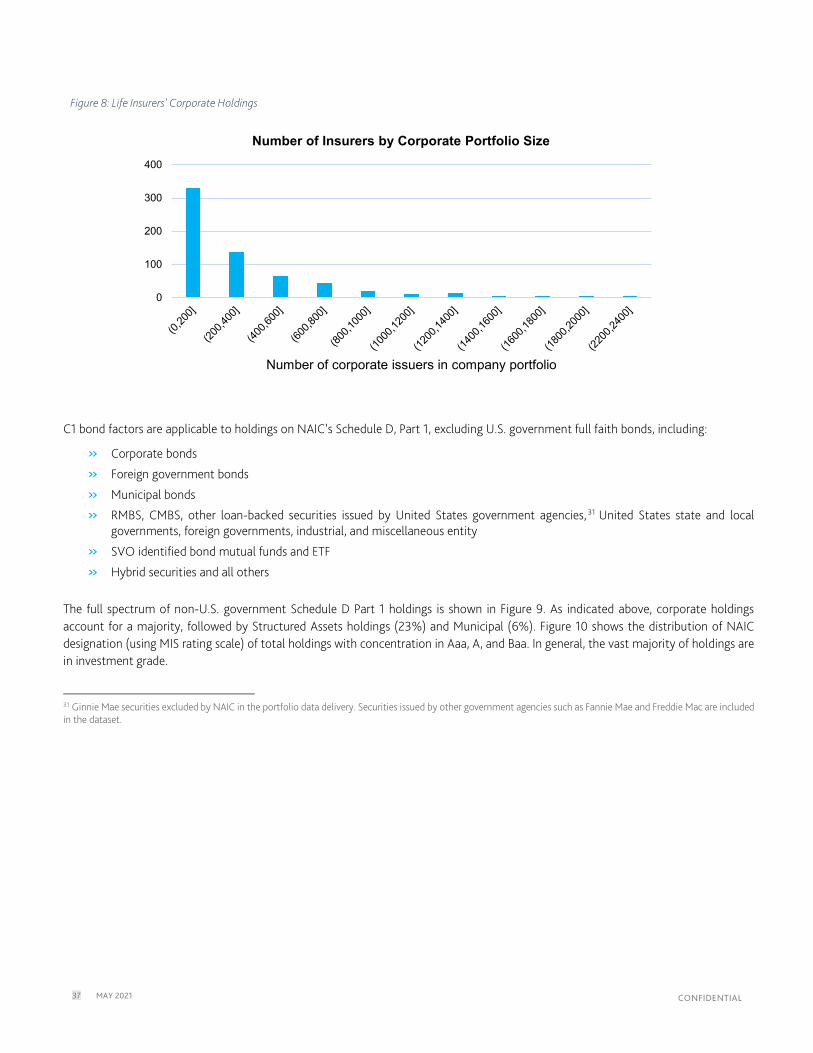
37 MAY 2021 CONFIDENTIAL
Figure 8: Life Insurers’ Corporate Holdings
C1 bond factors are applicable to holdings on NAIC’s Schedule D, Part 1, excluding U.S. government full faith bonds, including:
» Corporate bonds
» Foreign government bonds
» Municipal bonds
» RMBS, CMBS, other loan-backed securities issued by United States government agencies, 31 United States state and local governments, foreign governments, industrial, and miscellaneous entity
» SVO identified bond mutual funds and ETF
» Hybrid securities and all others
The full spectrum of non-U.S. government Schedule D Part 1 holdings is shown in Figure 9. As indicated above, corporate holdings account for a majority, followed by Structured Assets holdings (23%) and Municipal (6%). Figure 10 shows the distribution of NAIC designation (using MIS rating scale) of total holdings with concentration in Aaa, A, and Baa. In general, the vast majority of holdings are in investment grade.
31 Ginnie Mae securities excluded by NAIC in the portfolio data delivery. Securities issued by other government agencies such as Fannie Mae and Freddie Mac are included in the dataset.
0
100
200
300
400
Number of corporate issuers in company portfolio
Number of Insurers by Corporate Portfolio Size

38 MAY 2021 CONFIDENTIAL
Figure 9: Holding Amounts by Asset Class
Figure 10: Holding Amount by NAIC designation presented under MIS rating scale
Next, we explore each major asset class in the life insurers’ holdings: corporate, structured assets, and municipal credits.32 We present the NAIC designation distributions (using the MIS rating scale) of each asset class, which is instrumental in understanding the impact of the MA C1 Factors covered in Sections 5.2 and 5.3. For corporate holdings, we will also analyze the sector distribution, which is used in the development of MA’s default rate and LGD. Most corporate bond holdings fall under Baa, followed by A as seen in Figure 11. Holdings are concentrated in the lowest MIS ratings within the A and Aa categories. In contrast, within the Baa category, holdings are concentrated in Baa2. This finding is consistent with studies indicating underweighting of Baa3 by insurers to avoid credit downgrades that could result in a fallen angel reclassification from NAIC 2 to NAIC 3 resulting in a material increase in RBC under the current formula (Murray & Nikolova, 2019).
32 Corporate holdings include both public and private corporates.
66%
23%
6% 3% 2% 0% Corporate
Structured Assets
Municipal
Others
Foreign Government Bonds
SVO Identified funds
0
100
200
300
400
500
600
Aaa Aa1 Aa2 Aa3 A1 A2 A3 Baa1 Baa2 Baa3 Ba1 Ba2 Ba3 B1 B2 B3 Caa1 Caa2 Caa3
Hol
ding
Am
ount
($Bn
)
Rating
Holding Amount by Rating

39 MAY 2021 CONFIDENTIAL
Figure 11: Corporate Holdings by NAIC designation presented under MIS rating scale
Structured holdings comprise approximately 23% of the total Schedule D Part 1 holdings excluding U.S. government issues. Structured assets are classified by MA as holdings that fit into one of the following three types issued by entities other than the U.S. government: residential mortgage-backed securities (27%), commercial mortgage-backed securities (25%), and other loan-backed and structured securities (48%). Figure 12 displays the MIS rating composition of the structured assets. The majority of insurance structured holdings are rated Aaa, accounting for 47% of total holdings among all structured instruments in dollar amount. Figure 12: Structured Assets Holdings by NAIC designation presented under MIS rating scale
Municipal holdings account for 6.4% of the total in Schedule D Part 1 excluding U.S. government issues. They are generally highly rated, with the majority falling in Aaa, Aa, and A as seen in Figure 13. They are classified by MA as coming from subdivisions of individual possessions, states, and territories (direct and guaranteed). MA includes United States special revenue/assignment obligations as well.
050
100150200250300350400450500
Aaa Aa1 Aa2 Aa3 A1 A2 A3 Baa1 Baa2 Baa3 Ba1 Ba2 Ba3 B1 B2 B3 Caa1 Caa2 Caa3
Hol
ding
Am
ount
($Bn
)
Rating
0
50
100
150
200
250
300
350
400
Aaa Aa1 Aa2 Aa3 A1 A2 A3 Baa1 Baa2 Baa3 Ba1 Ba2 Ba3 B1 B2 B3 Caa1 Caa2 Caa3
Hol
ding
Am
ount
($Bn
)
Rating

40 MAY 2021 CONFIDENTIAL
Figure 13: Municipal Holdings by NAIC designation presented under MIS rating scale
We now transition and discuss the composition of corporate sector holdings as it compares with overall corporate issuance, and their respective properties, providing a rationale for sector-weighted default rates and LGD as discussed in Sections 4.2 and 4.4. Insurers’ U.S. corporate holdings, alongside U.S. issuers as covered by MA’s DRD by sector, are displayed as a percentage of total corporate in Table 16 along with respective default rates; over 80% of insurers’ corporate holdings with matching issuers in MA’s DRD are from U.S. issuers on a dollar basis.33
In Table 16, we compare the sector distributions of U.S. life insurers’ corporate holdings against the sector distribution of U.S. issuers in the data underlying (Moody's Investors Service, 2021), noting that differences therein suggest that the use of default rates from (Moody's Investors Service, 2021) without sector reweighting would not reflect the historical experience of life insurers’ U.S. corporate holdings. Table 16 shows that life insurers’ sector holdings vary by NAIC designation in the MIS rating scale, with Financials having a higher representation in investment grade, and Utilities holdings higher within the A range.34 Table 16 also shows differences between the sector distribution of life insurers’ holdings and issuance on which empirical default rates are constructed. Within the Aa rating’s category, for example, the proportion of financial issuers is 55.2%, while the proportion of life insurers’ financial holdings is 20.5%. Within the A rating’s category, the proportion of financial issuers is 36.2%, and the proportion of life insurers’ financial holdings is 23.6%. These differences persist for all rating’s categories between Aaa and Ca, highlighting the disparity between the sector composition of life insurers’ holdings and issuance, and suggesting that use of benchmark default rates from (Moody's Investors Service, 2021) (or derivatives thereof that ignore reweighting) would not reflect the historical experience of life insurers’ U.S. corporate holdings.
We investigate the driving sources behind some of these differences in Table 17, which compares the average remaining time to maturity (as of 12/31/2020) of U.S. corporate issues in life insurers’ holdings across different sectors. This is complemented by the average remaining time to maturity by sector of U.S. corporate issues. For example, we observe that the average time to maturity is lower for debt from the Financial sector (11.1 years for insurers’ U.S. corporate holdings, and 3.9 years for the universe of U.S. issues) than debt from the Industrial or Utility sectors (12.8-15.9 years for insurers’ U.S. corporate holdings, 11 years for the universe of U.S. issues), regardless of the pool considered. This aligns with the recognition that 1) shorter-term debt is often less suitable for life insurance duration matching, 2) Financial sector debt tends to exhibit shorter duration, and thus 3) life insurers hold proportionally less debt from
33 Approximately 60-80% of corporate holdings across different ratings are mapped to issuers in MA’s DRD by CUSIP. To remove the confounding effect of perpetual or extremely long-dated bonds, we excluded bonds with more than 30 years maturity in Table 17.
34 Given insurance company investment needs, it is perhaps not surprising the patterns look similar across the United States and Global samples.
0
5
10
15
20
25
30
35
40
45
Aaa Aa1 Aa2 Aa3 A1 A2 A3 Baa1 Baa2 Baa3 Ba1 Ba2 Ba3 B1 B2 B3 Caa1 Caa2 Caa3
Hol
ding
Am
ount
($Bn
)
Rating

41 MAY 2021 CONFIDENTIAL
the Financial sector than exists in the general market.35 Hence, MA empirical default rates and LGD distributions are reweighted across sectors to recognize the specific sector distribution of life insurers’ holdings, acknowledging that institutional features drive life insurers toward debt with different durations and, thus, sectors. With that, we acknowledge that there might be other characteristics beyond an issuer’s sector that further refine the analysis to allow estimated default rates and LGD to more closely reflect the historical experience of life insurers’ holdings.
Table 16: Comparing Life Insurers’ U.S. Corporate Holdings to U.S. Corporate Issuer Proportions by Corporates Sector 36
MIS Rating
U.S. Utility U.S. Industrial U.S. Financial
Sector as a Percentage of Life
Corporate Holdings
Proportion of Corporate Issuers
Attributed to Sector
Sector as a Percentage of Life
Corporate Holdings
Proportion of Corporate Issuers
Attributed to Sector
Sector as a Percentage of Life
Corporate Holdings
Proportion of Corporate Issuers
Attributed to Sector
Aaa 0.5% 5.9% 93.2% 42.9% 6.3% 51.2%
Aa 6.2% 8.3% 73.3% 36.5% 20.5% 55.2%
A 26.5% 17.8% 49.9% 46.0% 23.6% 36.2%
Baa 9.6% 21.2% 71.4% 58.1% 19.0% 20.7%
Ba 5.0% 5.9% 86.4% 81.5% 8.6% 12.6%
B 0.1% 1.0% 96.9% 92.8% 3.0% 6.2%
Caa 0.1% 0.6% 96.1% 95.6% 3.8% 3.9%
Ca 0.0% 1.1% 100.0% 90.4% 0.0% 8.5%
Overall 14.9% 10.4% 65.3% 68.1% 19. 8% 21.5%
35 See, for example, (The NAIC Capital Markets Bureau, 2021), that recognizes “Assets of life insurers are primarily invested in medium- and longer-term taxable fixed-income investments.” 36 Issuance proportions are computed from the MA DRD dataset based on counts of U.S. corporate issuers from an average of the 1983-2020 monthly cohorts underlying the calculation of MA’s empirical U.S. corporate by sector default rates, with cohort selection and counts computed under the same assumptions supporting default rates (see Appendix for details), where issuance denotes issuer counts not issuance volume.

42 MAY 2021 CONFIDENTIAL
Table 17: Average time to maturity of US corporate issues by sector
Sector Average Time to Maturity for life insurers’ U.S. corporate holdings
(notional weighted)
Average Time to Maturity for U.S. corporate issues
Proportion of Issuers Attributed to Sector
Financial 11.1 3.9 21.5%
Industrial 12.8 7.7 68.1%
Utility 15.9 11.0 10.4%
5.2 Impact of MA C1 Base Factors
In this section, we examine the impact MA RBC C1 base factors have on industry C1 RBC as compared to the Academy’s proposal. We start with the impact on the entire life insurance portfolio and then assess the impact on corporate, structured assets, and municipal credit. Due to the difference in NAIC designation distribution, C1 base RBC impact differs across asset classes. In the next section, we assess the combined impact of MA C1 base factors and the PAFs, enabling us to assess the PAFs’ incremental impact.
C1 base RBC under the current, MA’s, and Academy’s formulas are analyzed for each life company using the portfolio data described in Section 5.1. The left chart of Figure 14 shows the overall industry C1 base RBC for the entire portfolio of each life company, including Muni bonds and structured assets. We can see that under the current formula, the total industry required C1 base RBC across all life companies in our dataset is $38.53 billion. Under Academy’s proposal, that number rises to $49.03 billion. Under MA’s formula, the number is $46.34 billion, around 20% above the current level but lower than under the Academy’s proposal. The right chart of Figure 14 shows the industry C1 RBC segmented by the number of issuers in the portfolio.
Next, we assess the impact of C1 base factors on each asset class: corporate, structured assets, and municipal credits.
For corporate holdings, the C1 base RBC is $33.61 billion under MA’s formula, 26% higher than current and 5% lower than the Academy’s proposal, as seen in Figure 15. Most of the dollar C1 base RBC differences come from changes in the Baa MIS rating C1 base factors followed by A MIS rating C1 base factors due to the concentration of corporate holdings on these two sets of categories shown in Figure 11. The lower C1 base RBC under MA’s formula compared with the Academy is primarily driven by the lower proposed MIS investment grade C1 base factors (except Baa3). MA C1 base RBC is generally similar to the Academy’s for high yield.
For structured assets, the C1 base RBC is $5.84 billion under MA’s formula, 3% higher than current and 13% lower than the Academy’s proposal shown in Figure 16. As seen in Figure 12, most of the structured holdings fall under the Aaa MIS rating category, which has a lower base factor under MA’s formula as compared to the Academy’s proposal, driving the lower overall C1 base RBC. For investment grade, MA base RBC is generally lower than the Academy’s except Baa3. For high yield, MA base RBC is generally similar to the Academy’s.
For municipal, the C1 base RBC is $1.15 billion under MA’s formula, 14% higher than current and 21% lower than the Academy’s proposal displayed in Figure 17. As seen in Figure 13, most of the municipal holdings fall under Aaa/Aa/A MIS rating categories, which have lower base factors under MA’s formula as compared to the Academy’s proposal, driving the lower overall C1 base RBC.

43 MAY 2021 CONFIDENTIAL
Figure 14: C1 Base RBC Across Life Companies
Figure 15: C1 Base RBC Across Life Companies for Corporate Bond Holdings
38.53
49.0346.34
0
10
20
30
40
50
60
Billio
n ($
)
Total Industry C1 Base RBC Across Life Companies
Current Academy Proposal MA
0123456789
Billio
n ($
)Number of Issuers
C1 Base RBC Across Life Companies of Different Issuer Counts
Current Academy Proposal MA
26.65
35.333.61
0
5
10
15
20
25
30
35
40
Billio
n ($
)
Corporate Bond C1 Base RBC Acrooss Life Companies
Current Academy Proposal MA
0
1
2
3
4
5
6
Billio
n ($
)
Number of Issuers
C1 Base RBC Across Life Companies of Different Issuer Counts
Current Academy Proposal MA

44 MAY 2021 CONFIDENTIAL
Figure 16: C1 Base RBC Across Life Companies for Structured Asset Holdings
Figure 17: C1 Base RBC Across Life Companies for Municipal Credit Holdings
5.3 Impact of MA C1 Factors
In this section, we examine how the MA RBC C1 bond factors, the C1 base factors, and the PAFs affect industry C1 RBC, as compared to the Academy’s proposal. We find that MA’s C1 Factors increases overall industry C1 RBC by around 11%. The increase is fairly evenly distributed across portfolios with small-, medium- and large- number of issuers. In contrast, the Academy’s proposal increases the overall industry C1 RBC by 14%, with small- and medium-size companies experiencing the largest increase.
5.66
6.7
5.84
0
1
2
3
4
5
6
7
8
Billio
n ($
)
Structured Asset C1 Base RBC Acrooss Life Companies
Current Academy Proposal MA
00.20.40.60.8
11.21.41.6
Billio
n ($
)Number of Issuers
C1 Base RBC Across Life Companies of Different Issuer Counts
Current Academy Proposal MA
1.01
1.46
1.15
0
0.2
0.4
0.6
0.8
1
1.2
1.4
1.6
Billio
n ($
)
Municipal Credit C1 Base RBC Acrooss Life Companies
Current Academy Proposal MA
0
0.05
0.1
0.15
0.2
0.25
Billio
n ($
)
Number of Issuers
C1 Base RBC Across Life Companies of Different Issuer Counts
Current Academy Proposal MA

45 MAY 2021 CONFIDENTIAL
To examine and compare the impact of MA’s C1 Factors and the Academy’s proposals, we calculate the post-PAF RBC using the C1 base factors and PAFs under the current formula, MA’s formula, and the Academy’s proposal for each life company based on the portfolio data described in Section 4.7. The left chart of Figure 18 shows the overall industry C1 RBC level under different cases. While the PAFs are estimated using corporate bond data only, the impact analysis is conducted on the entire portfolio of each life company, including Muni bonds and structured assets. Under the current formula, the total industry required C1 RBC is $37.82 billion. Under the Academy’s proposal, that number increases to $43.19 billion. Under MA’s C1 Factors, the number is $41.83 billion, around 11% above the current level but lower than under the Academy’s proposal. The right chart of Figure 18 shows the industry C1 RBC segmented by the number of issuers in the portfolio. We can see that under Academy’s proposal, the industry’s C1 RBC increases from the current level for life companies with 2,500 or fewer issuers in particular. The increase, while still positive, is milder for companies with over 2,500 issuers. By contrast, under MA’s C1 Factors, the C1 RBC increases moderately across portfolios with a varying number of issuers.
Next, we assess the impact of post-PAF C1 RBC on each asset class, corporate and structured assets.
MA’s post-PAF C1 RBC for the corporate portfolio is $30.48 billion, 16% higher than current and 3% lower than the Academy’s proposal. This is driven by the concentrated holdings in A and Baa MIS rating categories, which face lower C1 base factors (other than Baa3) under MA’s formula compared to the Academy’s.
MA’s post-PAF C1 RBC for the structured portfolio is $5.26 billion, 5% lower than current and 10% lower than the Academy’s proposal. Lower post-PAF C1 RBC under MA’s formula is driven by structured asset holdings mostly falling under the Aaa MIS rating category, which has a lower C1 base factor under MA’s formula compared to both the Academy’s proposal and current. Figure 18: Total Post-PAF C1 RBC Across Life Companies
37.82
43.19 41.83
0
5
10
15
20
25
30
35
40
45
50
Billio
n ($
)
Total Industry Post-PAF C1 RBC Across Life Companies
Current Academy Proposal MA
012345678
Billio
n ($
)
Number of Issuers
Post-PAF C1 Base RBC Across Life Companies of Different Issuer Counts
Current Academy Proposal MA
46 MAY 2021 CONFIDENTIAL
Figure 19: Total Post-PAF C1 RBC Across Life Companies for Corporate Bond Holdings
Figure 20: Total Post-PAF C1 RBC Across Life Companies for Structured Asset Holdings
26.28
31.32 30.48
0
5
10
15
20
25
30
35
Billio
n ($
)
Corporate Bond Post-PAF C1 RBC Across Life Companies
Current Academy Proposal MA
0
1
2
3
4
5
6
Billio
n ($
)Number of Issuers
Post-PAF C1 Base RBC Across Life Companies of Different Issuer Counts
Current Academy Proposal MA
5.555.86
5.26
0
1
2
3
4
5
6
7
Billio
n ($
)
Structured Asset Post-PAF C1 RBC Across Life Companies
Current Academy Proposal MA
0
0.2
0.4
0.6
0.8
1
1.2
1.4
Billio
n ($
)
Number of Issuers
Post-PAF C1 Base RBC Across Life Companies of Different Issuer Counts
Current Academy Proposal MA

47 MAY 2021 CONFIDENTIAL
6 Targeted Modifications and Sensitivity Analysis
This section provides a recap of targeted modifications and their impact on the C1 base factors. In addition, this section presents the sensitivity analysis of the key parameters to the model.
6.1 Recap of Targeted Modifications to the Base Factors
As discussed in Section 2, the marginal impact of each targeted modification is assessed by applying each modification sequentially and in the following order, with the initial point of reference being the C1 factors proposed by the Academy:37
1. Replicate the Academy’s proposed factors
2. Fixed PD-LGD correlation error in the simulation engine
3. Update discount rate and tax rate
4. Update the LGD distribution
5. Set Risk Premium to expected loss plus 0.5 standard deviation
6. Introduce the MA correlation model
7. Update the baseline PD default rate term structure with MA’s default rate term structure. As discussed in Section 4, the impact of each targeted modification on C1 base factors is displayed in Table 4, and summarized as follows:
» Correction of replicated Academy simulation engine has a mild impact
» Updating the discount rate and tax rate has a mild impact
» Updating LGD distribution moderately lowers the C1 factors for investment grade and has an insignificant effect on high yield
» Setting the Risk Premium to expected loss plus 0.5 standard deviation reduces C1 factors, and mildly increases their slope
» Replacing the economic state model with the MA correlation model generally increases C1 factors and increases their slope
» MA’s default rates generally decrease C1 factors and increase their slope
37 Replication was based on the methodology paper and letters (American Academy of Actuaries, 2015)

48 MAY 2021 CONFIDENTIAL
Figure 21: C1 RBC Base Factors for Different Targeted Modifications
6.2 Sensitivity Analysis
This section centralizes the reporting of sensitivity analysis that is referenced in each respective section. The analysis provides transparency by articulating the economic implications of model and parameter choices. Sensitivity analysis is conducted on the following parameters:
» Discount rate
» LGD
» Risk Premium
» Target Probability (that is the percentile corresponding to the safety or confidence level)
» Correlations
» Simulation Seeds
0.0%
0.5%
1.0%
1.5%
2.0%
2.5%
Aaa Aa1 Aa2 Aa3 A1 A2 A3 Baa1 Baa2 Baa3
Investment Grade(1) Current
(2) Academy Proposal [March 2021]
(3) MA's Replication Under AcademyParameters and Settings
(4): (3) + Corrected Simulation Engine
(5): (4) + MA’s Discount Rate, Tax Rate
(6): (5) + MA’s LGD Distribution
(7): (6) + Risk Premium at mean + 0.5 SD
(8): (7) + Economic State Model Replacedwith Correlation Model
(9) MA: (8) + MA’s Default Rates
0.0%
5.0%
10.0%
15.0%
20.0%
25.0%
30.0%
35.0%
40.0%
Ba1 Ba2 Ba3 B1 B2 B3 Caa1 Caa2 Caa3
High-Yield(1) Current
(2) Academy Proposal [March 2021]
(3) MA's Replication Under AcademyParameters and Settings
(4): (3) + Corrected Simulation Engine
(5): (4) + MA’s Discount Rate, Tax Rate
(6): (5) + MA’s LGD Distribution
(7): (6) + Risk Premium at mean + 0.5 SD
(8): (7) + Economic State Model Replacedwith Correlation Model
(9) MA: (8) + MA’s Default Rates

49 MAY 2021 CONFIDENTIAL
Parameter choices are summarized in Table 18. When running sensitivity analysis for one parameter, all other parameters remain as those under MA’s targeted modifications. Table 18: Key Parameters of RBC C1 Model
PD Term Structure Simulation Model Risk Premium
Discount Rate Tax Rate LGD Distribution
Target Probability
Simulation Seeds
Proposed by Academy
Academy's smoothed Default Rates
Economic state model
Expected Loss 5% 21% Academy's LGD Distribution (1987-2012)
96% Unknown. Limited documentation
MA MA Default Rates
Correlation model with RSQ =10%
Expected Loss + 0.5 standard deviation
3.47% 21% MA LGD Distribution (1987-2019)
96% Seed 1
Parameters Tested in the Sensitivity Analysis
Correlation RSQ = 5%, 7.5% 12.5%
Expected Loss + 1 standard deviation
2.25%, 4.32%
LGD: Academy’s proposed and MA’s LGD
92%, 93%, 94%, 95%
Seed 2 - 10
6.2.1 Discount Rate
Section 4.1 discusses data sources and time windows for discount rate estimation. The MA C1 base factors are estimated with a pretax discount rate of 3.47% (and a tax rate of 21%). To assess the sensitivity of the C1 base factors to the discount rate, we explore the pretax discount rate estimated over varying time windows. As seen in Figure 22, a lower discount rate leads to higher C1 factors; the present value of future losses is higher. C1 factors for investment grade are slightly more sensitive, in general, to the discount rate than for high-yield on a relative basis. Compared with the pretax discount rate of 3.47%, discount rates estimated over other windows have the following mild effect on the C1 base factors on a relative basis:
» 1993−2013 used by the Academy (5%): results in a decrease of 6%-7% for investment grade, and 3%-6% for high-yield
» 1993−2020 (4.32%): results in a decrease of 2%-6% for investment grade, and 2%-3% for high-yield
» 2010−2020 (2.25%): results in an increase of 5%-7% for investment grade, and 3%-5% for high-yield
Figure 22: C1 RBC Base Factors for different discount rates
6.2.2 LGD Section 4.2 discusses target modifications to LGD. In this section, we assess the sensitivity of C1 base factors to the Academy’s and MA’s LGD. MA’s LGD distributions have a slightly lower mean of 52%, compared to the Academy’s proposed 53%, leading to a mild decrease in C1 base factors relative to the Academy’s, as seen in Figure 23.
0.0%
0.5%
1.0%
1.5%
2.0%
2.5%
Aaa Aa1 Aa2 Aa3 A1 A2 A3 Baa1 Baa2 Baa3
Investment Grade
0.0%
10.0%
20.0%
30.0%
40.0%
Ba1 Ba2 Ba3 B1 B2 B3 Caa1 Caa2 Caa3
High-Yield
Discount rate5%
Discount rate4.32%
Discount rate3.47%
Discount rate2.25%

50 MAY 2021 CONFIDENTIAL
Figure 23: Impact of LGD Updates on C1 Base Factors
6.2.3 Risk Premium In Section 4.3, we assess the sensitivity of C1 base factors to the various Risk Premium options as follows:
» Expected loss (used by the Academy)
» Expected loss plus 0.5 standard deviation (used by MA)
» Expected loss plus 1 standard deviation As seen in Figure 24, a higher level of Risk Premium leads to lower C1 base factors, as more losses are covered by Risk Premium. On a relative basis, C1 factors for investment grade are more sensitive than below investment grade.
Figure 24: C1 Base Factors for different levels of Risk Premium
6.2.4 Target Probability The target probability, that is the percentile corresponding to the safety or confidence level, is the level of loss that C1 RBC covers expressed as a percentile of the loss distribution. In this section, and unless stated otherwise, we use “%” to indicate “percentile”. For the MA C1 factors, we retain the target probability (96%) used by the Academy in the 2017 and 2021 updates. While we do not propose a change to the target probability, assessing its impact on C1 base factors would facilitate comprehensive thinking of the C1 RBC framework. Target probabilities in the sensitivity analysis are set to 92%, 93%, 94%, 95% and 96% recognizing that:
» Lower-bound 92% is the assumption in NAIC’s review of C1 factors in 2002
» Higher-bound 96% (used by MA) is the target probability selected by the Academy in 2017 and 2021 updates
0.0%
0.5%
1.0%
1.5%
2.0%
2.5%
Aaa Aa1 Aa2 Aa3 A1 A2 A3 Baa1Baa2Baa3
Investment Grade
Academy Proposal LGD MA LGD
0.0%
10.0%
20.0%
30.0%
40.0%
Ba1 Ba2 Ba3 B1 B2 B3 Caa1Caa2Caa3
High-Yield
Academy Proposal LGD MA LGD
0.0%
1.0%
2.0%
3.0%
Aaa Aa1 Aa2 Aa3 A1 A2 A3 Baa1Baa2Baa3
Investment Grade
Expected LossExpected Loss + 0.5 standard deviationExpected Loss + 1 standard deviation
0.0%
10.0%
20.0%
30.0%
40.0%
Ba1 Ba2 Ba3 B1 B2 B3 Caa1Caa2Caa3
High-Yield
Expected LossExpected Loss + 0.5 standard deviationExpected Loss + 1 standard deviation

51 MAY 2021 CONFIDENTIAL
As seen in Figure 25, higher target probability leads to higher C1 factors, as more capital is required to cover higher tail loss. C1 factors for MIS ratings in the higher end of the spectrum are more sensitive to the target probability on a relative basis. Figure 25: C1 RBC Base Factors for different Target Probabilities
6.2.5 Correlations
In Section 4.5.2, we introduced the Gaussian Copula-based correlation model, which MA parameterizes with an RSQ value of 10%. To assess the sensitivity of post-PAF C1 RBC to the RSQ value, we explore three other values in addition to 10%: (1) RSQ = 5%, which was calibrated to the economic state model with Academy proposed parameters; (2) 7.5%; and (3) 12.5%. The results are presented in the figure below. The overall RBC increases from $41.83 to $48.02 billion with a higher RSQ value of 12% (more correlated losses, less diversification benefits), declines to $36.42 billion with the lower RSQ value of 7.5% (more diversification benefits), and further declines to $32.17 billion with the RSQ value of 5% calibrated to the economic state model. The analysis illustrates the importance of the correlation parameterization—varying the RSQ value even within the range of 5% to 12.5% can change RBC by 15% to 20% from the level of $41.83 billion and should not be set in isolation without consideration of other parameter choices.
Figure 26: Correlation sensitivity analysis. Post-PAF C1 RBC for four levels of the RSQ value
0.0%
0.5%
1.0%
1.5%
2.0%
2.5%
Aaa Aa1 Aa2 Aa3 A1 A2 A3 Baa1 Baa2 Baa3
Investment Grade
92% target probability 93% target probability94% target probability 95% target probability96% target probability
0.0%
10.0%
20.0%
30.0%
40.0%
Ba1 Ba2 Ba3 B1 B2 B3 Caa1 Caa2 Caa3
High-Yield
92% target probability 93% target probability94% target probability 95% target probability96% target probability
37.8243.19
32.1736.42
41.8348.02
0
10
20
30
40
50
60
Billio
n ($
)
Total Post-PAF C1 RBC Across Life Companies
Current Academy Proposal
MA with RSQ Calibrated to ES Base Factors MA with RSQ = 7.5%
MA MA with RSQ = 12.5%

52 MAY 2021 CONFIDENTIAL
6.2.6 Simulation Seeds
This report presents C1 base factors that are calculated using 10,000 simulation trials, the same as the Academy’s proposal, and subject to simulation noise. To examine the impact of simulation noise on the MA C1 base factors, C1 base factors are re-estimated under 10 different pseudo-random number-generating starting seeds. The resulting base factors across these 10 runs are reported in Table 19. In addition, the table reports mean and standard deviation of the C1 base factors across the starting seeds, with relatively mild differences across starting seeds. Table 19: C1 Base Factors under Different Seeds
MIS Rating Seed 1 Seed 2 Seed 3 Seed 4 Seed 5 Seed 6 Seed 7 Seed 8 Seed 9 Seed 10 Mean SD
Aaa 0.158% 0.163% 0.149% 0.148% 0.152% 0.170% 0.159% 0.158% 0.158% 0.152% 0.157% 0.0060%
Aa1 0.271% 0.274% 0.271% 0.256% 0.271% 0.280% 0.261% 0.272% 0.269% 0.266% 0.269% 0.0062%
Aa2 0.419% 0.439% 0.435% 0.431% 0.440% 0.440% 0.425% 0.434% 0.429% 0.430% 0.432% 0.0063%
Aa3 0.523% 0.543% 0.548% 0.529% 0.540% 0.537% 0.512% 0.523% 0.541% 0.534% 0.533% 0.0101%
A1 0.657% 0.643% 0.661% 0.655% 0.654% 0.660% 0.661% 0.653% 0.672% 0.663% 0.658% 0.0069%
A2 0.816% 0.835% 0.833% 0.831% 0.814% 0.809% 0.824% 0.825% 0.820% 0.816% 0.823% 0.0080%
A3 1.016% 1.015% 0.987% 0.997% 0.983% 1.000% 0.981% 0.989% 0.999% 1.010% 0.998% 0.0114%
Baa1 1.261% 1.248% 1.266% 1.220% 1.258% 1.243% 1.263% 1.232% 1.246% 1.194% 1.243% 0.0205%
Baa2 1.523% 1.549% 1.504% 1.529% 1.582% 1.545% 1.528% 1.558% 1.559% 1.521% 1.540% 0.0208%
Baa3 2.168% 2.160% 2.162% 2.145% 2.180% 2.187% 2.217% 2.174% 2.182% 2.157% 2.173% 0.0182%
Ba1 3.151% 3.074% 3.115% 3.136% 3.114% 3.153% 3.140% 3.177% 3.165% 3.070% 3.130% 0.0327%
Ba2 4.537% 4.726% 4.633% 4.686% 4.711% 4.630% 4.662% 4.689% 4.616% 4.673% 4.656% 0.0498%
Ba3 6.017% 5.913% 5.707% 5.874% 5.797% 5.798% 5.795% 5.916% 5.929% 5.747% 5.849% 0.0866%
B1 7.386% 7.423% 7.340% 7.586% 7.400% 7.393% 7.487% 7.410% 7.342% 7.439% 7.421% 0.0654%
B2 9.535% 9.823% 9.394% 9.174% 9.343% 9.509% 9.250% 9.549% 9.409% 9.360% 9.435% 0.1644%
B3 12.428% 12.316% 12.450% 12.436% 12.458% 12.404% 12.779% 12.377% 12.340% 12.349% 12.434% 0.1183%
Caa1 16.942% 16.936% 16.465% 17.090% 16.853% 16.614% 17.048% 17.000% 16.688% 17.012% 16.865% 0.1881%
Caa2 23.798% 23.473% 23.318% 23.320% 23.597% 23.212% 23.161% 23.457% 23.307% 24.011% 23.466% 0.2433%
Caa3 32.975% 32.771% 33.144% 32.444% 33.272% 32.919% 32.981% 33.185% 33.214% 32.798% 32.970% 0.2288%

53 MAY 2021 CONFIDENTIAL
7 Suggested Next Steps
As discussed in the Executive Summary, this report was written as requested by the ACLI, in conjunction with the NAIC. This report presents MA targeted modifications to the C1 base factors and PAFs that help “identify potentially weakly capitalized companies” by utilizing minimum capital standards that reflect differentiated risks across MIS rating categories and across portfolios with a varying number of issuers. The MA C1 Factors are based on an objective assessment of supporting documentation, data that reflect historical experience of life insurers’ holdings, and modeling approaches that in MA's judgment and experience, are viewed as best practices and appropriate for use in calculating C1 factors. The performance criteria are heuristic, given the inherent challenge of the RBC C1 framework. MA’s findings must be taken within the context of the Scope and limits to MA’s RBC impact analysis that does not consider factors such as shifts in life holdings that may arise, in part, as a result of the MA C1 Factors being adopted. This report provides transparency by articulating the limitations to the underlying data, methodologies and, ultimately, to the MA C1 Factors themselves.
With these aspects in mind, MA recommends that the regulators and the NAIC review the targeted modifications described in this study. While it is ultimately for the NAIC to determine whether, and to what extent, to use the MA methodologies and MA C1 Factors in setting the final C1 factors, the NAIC should understand that the modeling framework and parameters on which the factors are based rely on interconnected elements that give the factors consistency. If the NIAC NAIC decides to pursue piecemeal adoption or isolated adjustments to the MA C1 Factors, it must do so with the understanding that the benefits of the methodology MA pursued in deriving the factors and their consistency will be potentially compromised.
In addition, MA recommends the NAIC consider a broader reevaluation of the RBC C1 factors, recognizing the lead time needed for data collection and research, that should be approached in conjunction with all stakeholders iteratively, as follows:
» Obtain clarity and agreement on the desired level of
- Model complexity (for example, issuer concentration)
- Granularity (for example, differentiating risks across asset classes)
» Assess the cost implications
- Resources, including personnel, to develop and implement models within a sound model risk management framework
- Data collection
- Model monitoring and model re-development -
» Assess the implications, both cost and design, of the current NAIC RBC structure regarding the exhibits and interaction with other RBC factors
» Articulate governance of any redesign—potentially impacting organizational structure at life insurance companies and NAIC
» Control mechanisms through policies and procedures associated with model development, validation, implementation and use
» Propose redesigned C1 factors
- Assess and agree on performance criteria, along with possible data sources and methodologies
- Propose updated model and C1 factors, recognizing benchmarking and validation concerns, including model limitations, and adhering to sound model risk management guidelines (Board of Governors of the Federal Reserve System and Office of the Comptroller of the Currency , 2011)
- Assess implications for assessment of insolvency risk across the life insurance industry

54 MAY 2021 CONFIDENTIAL
8 Appendix
This Appendix contains technical details related to MA’s C1 Factors. Section 8.1 describes the methodology used in constructing the empirical default rates underpinning MA’s proposed baseline default rates. Section 8.2 details MA’s procedure for converting empirical default rates to baseline default rates, described broadly in Section 4.4. Section 8.3 provides the technical details underpinning the PAFs discussed broadly in Section 4.7. Section 8.4 summarizes MA’s review of the concentration factor (doubling of top-ten holdings), which is not part of MA’s C1 Factors.
8.1 Default Rate Methodology
This Appendix compares MA’s and MIS’ methodologies pertaining to the processing of default rates.
The tables below display empirical average cumulative default rates for global corporates for the period of 1983−2020 and for tenors of 1 year to 10 years. The first table contains empirical default rates produced by the MIS and published in Exhibit 42 of the MIS Sector In-Depth Report, (Moody's Investors Service, 2021). The second table contains empirical default rates determined by MA using the method that is employed to produce U.S. sector-level corporate default rates for the C1 factor calculations in this report (the specific usage of these sector-level corporate default rates is discussed in Section 4.4.2). The purpose of the comparison of the two tables below is to assess the materiality and reasons for any remaining differences between the figures published by MIS and those computed by MA. Table 20: Average cumulative default rates for global corporates, from 1983-2020, as published by MIS and calculated by MA
MIS Annual default study, January 28, 2021, Exhibit 42
MIS Rating \Year 1 2 3 4 5 6 7 8 9 10
Aaa 0.000% 0.012% 0.012% 0.035% 0.062% 0.092% 0.125% 0.127% 0.127% 0.127%
Aa 0.022% 0.061% 0.112% 0.197% 0.301% 0.393% 0.485% 0.564% 0.645% 0.729%
A 0.053% 0.163% 0.344% 0.529% 0.757% 1.010% 1.273% 1.546% 1.807% 2.065%
Baa 0.156% 0.400% 0.695% 1.043% 1.405% 1.794% 2.164% 2.546% 2.947% 3.362%
Ba 0.830% 2.347% 4.141% 6.045% 7.767% 9.380% 10.857% 12.229% 13.573% 14.943%
B 3.211% 7.733% 12.437% 16.714% 20.579% 23.992% 26.999% 29.654% 32.057% 34.134%
Caa-C 9.819% 17.606% 24.310% 30.164% 35.243% 39.479% 43.061% 46.259% 49.191% 51.598% MA empirical default rates replication from DRD database
MIS Rating \Year 1 2 3 4 5 6 7 8 9 10
Aaa 0.000% 0.012% 0.012% 0.035% 0.062% 0.092% 0.125% 0.128% 0.128% 0.128%
Aa 0.022% 0.061% 0.112% 0.197% 0.301% 0.392% 0.484% 0.564% 0.645% 0.728%
A 0.053% 0.164% 0.345% 0.530% 0.758% 1.012% 1.276% 1.549% 1.810% 2.069%
Baa 0.156% 0.400% 0.695% 1.044% 1.408% 1.797% 2.173% 2.560% 2.968% 3.392%
Ba 0.846% 2.370% 4.167% 6.073% 7.792% 9.403% 10.869% 12.226% 13.556% 14.920%
B 3.252% 7.780% 12.475% 16.739% 20.587% 23.986% 26.992% 29.646% 32.045% 34.125%
Caa-C 9.753% 17.534% 24.249% 30.077% 35.122% 39.336% 42.923% 46.133% 49.067% 51.507%
Focusing on the magnitude of differences, the tables imply that for categories Aaa, Aa, and A, the maximum absolute deviation of the MA figures from the MIS figures is 0.003%. For Baa, Ba, and B categories, the deviation does not exceed 0.047%, and for the Caa-C categories 0.143%. That magnitude of differences remains within reason.

55 MAY 2021 CONFIDENTIAL
There are several reasons for these residual differences. First, while both tables are based on a global sample of corporates with senior unsecured MIS rating (actual or estimated), there can be borderline cases of issuers that are included in the sample for one table but not the other. Second, the treatment of a withdrawn MIS rating is an important consideration. For all cohorts across time, the MA calculation uses the same method of dealing with MIS rating withdrawals, as described in (Moody's Investors Service, 2006). In particular, MA’s U.S. corporates empirical default rates, grouped by sector, are created from MA’s DRD data; based on MIS senior unsecured rating for long-term issuances; filter out issuers in structured finance, project finance, and public-private partnerships to reflect corporate issuances; and limited to U.S. issuers. These empirical default rates are presented at the 10-year in Table 16 and Table 8, and they directly inform MA’s baseline empirical default rates, as described in Appendix Section 8.2. Over the decades included in the calculation, however, the treatment of withdrawn MIS rating by MIS has evolved, and the table with figures from MIS reflects this fact.38 Finally, there may remain subtle differences in some aspects of cohort formation.
8.2 Constructing Baseline Default Rates
We describe the methodology for constructing the baseline default rates of Section 4.4 in full. The methodology consists of three steps. In Step 1, we describe the process for obtaining sector-weighted cumulative empirical default rates for coarse ratings categories. These will be inputs into the anchors for MA’s baseline default rates for selected ratings and points surrounding the term structure. In Step 2, we describe adjustments made to the empirical default rates from Step 1 for their use in anchoring. This includes: an adjustment to reconcile the imbalance in the issuance of alphanumeric ratings within each coarse ratings category with the exponential structure of default rates across ratings; an adjustment to extrapolate the cumulative default rate (henceforth, CDR) for Aaa; and the use of a conservative benchmark to anchor for Caa3. In Step 3, we describe the process of interpolating across the term structure and between unanchored ratings. In particular, we interpolate the term structure for anchored ratings by scaling and rotating the empirical term structure for corresponding coarse ratings from benchmarks, and we interpolate for alphanumeric ratings between anchored ratings via geometric means. Notation We refer to the following notation throughout this section:
» Let 𝐴𝐴𝑅𝑅 =
{𝐴𝐴𝐴𝐴𝐴𝐴,𝐴𝐴𝐴𝐴1,𝐴𝐴𝐴𝐴2,𝐴𝐴𝐴𝐴3,𝐴𝐴1,𝐴𝐴2,𝐴𝐴3,𝐵𝐵𝐴𝐴𝐴𝐴1,𝐵𝐵𝐴𝐴𝐴𝐴2,𝐵𝐵𝐴𝐴𝐴𝐴3,𝐵𝐵𝐴𝐴1,𝐵𝐵𝐴𝐴2,𝐵𝐵𝐴𝐴3,𝐵𝐵1,𝐵𝐵2,𝐵𝐵3,𝐶𝐶𝐴𝐴𝐴𝐴1,𝐶𝐶𝐴𝐴𝐴𝐴2,𝐶𝐶𝐴𝐴𝐴𝐴3}
denote the set of MIS alphanumeric rating categories, and let 𝑘𝑘 ∈ 𝐴𝐴𝑅𝑅 denote the index of a particular MIS rating Let 𝐶𝐶𝑅𝑅 ∈ {𝐴𝐴𝐴𝐴𝐴𝐴,𝐴𝐴𝐴𝐴,𝐴𝐴,𝐵𝐵𝐴𝐴𝐴𝐴,𝐵𝐵𝐴𝐴,𝐵𝐵,𝐶𝐶𝐴𝐴𝐴𝐴,𝐶𝐶𝐴𝐴} denote the set of coarse MIS rating categories, and let 𝑖𝑖 ∈ 𝐶𝐶𝑅𝑅 denote the index of a particular MIS rating. For each 𝑖𝑖 ∈ {𝐴𝐴𝐴𝐴,𝐴𝐴,𝐵𝐵𝐴𝐴𝐴𝐴,𝐵𝐵𝐴𝐴,𝐵𝐵,𝐶𝐶𝐴𝐴𝐴𝐴}, let 𝐾𝐾𝑖𝑖 denote the set of MIS alphanumeric ratings associated to 𝑖𝑖:
𝐾𝐾𝐴𝐴𝐴𝐴 = {𝐴𝐴𝐴𝐴1,𝐴𝐴𝐴𝐴2,𝐴𝐴𝐴𝐴3} 𝐾𝐾𝐴𝐴 = {𝐴𝐴1,𝐴𝐴2,𝐴𝐴3}
𝐾𝐾𝐵𝐵𝐴𝐴𝐴𝐴 = {𝐵𝐵𝐴𝐴𝐴𝐴1,𝐵𝐵𝐴𝐴𝐴𝐴2,𝐵𝐵𝐴𝐴𝐴𝐴3} 𝐾𝐾𝐵𝐵𝐴𝐴 = {𝐵𝐵𝐴𝐴1,𝐵𝐵𝐴𝐴2,𝐵𝐵𝐴𝐴3} 𝐾𝐾𝐵𝐵 = {𝐵𝐵1,𝐵𝐵2,𝐵𝐵3}
𝐾𝐾𝐶𝐶𝐴𝐴𝐴𝐴 = {𝐶𝐶𝐴𝐴𝐴𝐴1,𝐶𝐶𝐴𝐴𝐴𝐴2,𝐶𝐶𝐴𝐴𝐴𝐴3}
» Let 𝑡𝑡 ∈ {1, … ,10} denote tenor
» Let 𝑠𝑠 ∈ {Financial, Utility, Industrial} = 𝑅𝑅 denote sector The goal is to produce 𝐶𝐶𝑃𝑃𝐷𝐷𝑘𝑘,𝑡𝑡
MA, a set of MA’s baseline cumulative default rates for tenor 𝑡𝑡 and MIS alphanumeric rating 𝑘𝑘
38 The latest treatment of withdrawals can be found in (Moody's Investors Service, 2015)

56 MAY 2021 CONFIDENTIAL
Step 1: Generate empirical cumulative default rates » From MA’s DRD data, MA produces:
- Empirical cumulative default rates 𝐶𝐶𝑃𝑃𝐷𝐷𝑖𝑖,𝑡𝑡,𝑠𝑠
Emp for each coarse MIS ratings 𝑖𝑖, tenor 𝑡𝑡, sector 𝑠𝑠 (corresponding to the default rates underlying Table 16 and Table 8)
- Marginal distributions of life issuers’ (U.S. corporate) holdings over 𝑘𝑘 ∈ 𝐴𝐴𝑅𝑅, given by ℎ𝑘𝑘𝑚𝑚 . The values ℎ𝑘𝑘𝑚𝑚 sum to 1 over
𝑘𝑘 ∈ 𝐴𝐴𝑅𝑅
- Conditional distributions of life issuers’ (U.S. corporate) holdings over 𝑠𝑠 ∈ {Financial, Utility, Industrial} and 𝑘𝑘 ∈ 𝐴𝐴𝑅𝑅, denoted by ℎ𝑘𝑘,𝑠𝑠
𝑐𝑐
- Conditional distributions of life issuers’ (U.S. corporate) holdings over 𝑠𝑠 ∈ {Financial, Utility, Industrial} and 𝑖𝑖 = 𝐶𝐶𝐴𝐴, denoted by ℎ𝑖𝑖,𝑠𝑠𝑐𝑐
- For 𝑘𝑘 ∈ 𝐴𝐴𝑅𝑅, we calculate sector weights 𝑤𝑤𝑘𝑘,𝑠𝑠 as follows:
o For 𝑖𝑖 ∈ {𝐴𝐴𝐴𝐴,𝐴𝐴,𝐵𝐵,𝐵𝐵𝐴𝐴𝐴𝐴,𝐵𝐵𝐴𝐴,𝐵𝐵} and 𝑠𝑠 ∈ 𝑅𝑅, determine weights 𝑤𝑤𝑖𝑖,𝑠𝑠 =∑ �ℎ𝑘𝑘′
𝑚𝑚×ℎ𝑘𝑘′,𝑠𝑠𝑐𝑐 �𝑘𝑘′∈𝐾𝐾𝑖𝑖
∑ ∑ �ℎ𝑘𝑘′𝑚𝑚×ℎ𝑘𝑘′,𝑠𝑠′
𝑐𝑐 �𝑠𝑠′∈𝑆𝑆𝑘𝑘′∈𝐾𝐾𝑖𝑖
o For 𝑖𝑖 = 𝐶𝐶𝐴𝐴 and 𝑠𝑠 ∈ 𝑅𝑅, determine weights 𝑤𝑤𝑖𝑖 ,𝑠𝑠 =ℎ𝑖𝑖𝑚𝑚×ℎ𝑖𝑖,𝑠𝑠
𝑐𝑐
∑ ℎ𝑖𝑖𝑚𝑚×ℎ𝑖𝑖,𝑠𝑠′
𝑐𝑐𝑠𝑠′∈𝑆𝑆
» For each sector 𝑠𝑠 ∈ 𝑅𝑅 and coarse MIS rating 𝑖𝑖 ∈ {𝐴𝐴𝐴𝐴,𝐴𝐴,𝐵𝐵,𝐵𝐵𝐴𝐴𝐴𝐴,𝐵𝐵𝐴𝐴,𝐵𝐵,𝐶𝐶𝐴𝐴}, we calculate the sector-weighted marginal default
rate 𝑀𝑀𝑃𝑃𝐷𝐷𝑖𝑖,𝑡𝑡,𝑠𝑠Emp = 1 − �1 − 𝐶𝐶𝑃𝑃𝐷𝐷𝑖𝑖,𝑡𝑡,𝑠𝑠
Emp� ÷ �1 − 𝐶𝐶𝑃𝑃𝐷𝐷𝑖𝑖,𝑡𝑡−1,𝑠𝑠Emp �
» We aggregate 𝑀𝑀𝑃𝑃𝐷𝐷𝑖𝑖 ,𝑡𝑡,𝑠𝑠
Emp into 𝑀𝑀𝑃𝑃𝐷𝐷𝑖𝑖,𝑡𝑡Emp by applying a weighted sum over sector weights, given by 𝑀𝑀𝑃𝑃𝐷𝐷𝑖𝑖,𝑡𝑡
Emp =∑ 𝑤𝑤𝑖𝑖,𝑠𝑠′ × 𝑀𝑀𝑃𝑃𝐷𝐷𝑖𝑖 ,𝑡𝑡,𝑠𝑠′
Emp𝑠𝑠′∈𝑆𝑆
» We convert 𝑀𝑀𝑃𝑃𝐷𝐷𝑖𝑖 ,𝑡𝑡
Emp to 𝐶𝐶𝑃𝑃𝐷𝐷𝑖𝑖 ,𝑡𝑡Emp recursively:
𝐶𝐶𝑃𝑃𝐷𝐷𝑖𝑖 ,1
Emp = 𝑀𝑀𝑃𝑃𝐷𝐷𝑖𝑖,1Emp, 𝐶𝐶𝑃𝑃𝐷𝐷𝑖𝑖,𝑡𝑡
Emp = 1 − �1 − 𝐶𝐶𝑃𝑃𝐷𝐷𝑖𝑖,𝑡𝑡−1Emp� × �1 −𝑀𝑀𝑃𝑃𝐷𝐷𝑖𝑖 ,𝑡𝑡
Emp�
Step 2: Set anchoring
» Let 𝐶𝐶𝑃𝑃𝐷𝐷𝑘𝑘,𝑡𝑡E43 denote the cumulative default probability for tenor 𝑡𝑡 ∈ {10,1} and MIS rating 𝑘𝑘 from Exhibit 43 of (Moody's
Investors Service, 2021), noting that MIS rating Caa is substituted for granular MIS ratings Caa1-Caa3 in Exhibit 43
» Fit parameters 𝛼𝛼�10, 𝛾𝛾�10 using log(𝑦𝑦) = log(𝛼𝛼) + 𝛾𝛾𝛾𝛾 to the following data with outcome variable 𝑦𝑦 and explanatory variable 𝛾𝛾 as follows:39
39 Aaa outcome variable is adjusted by 2/3 to reflect that Gettys Oil and Texaco comprised 1/3 of the global sample of defaults.
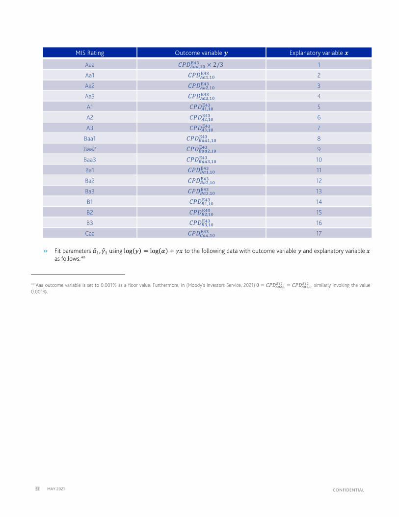
57 MAY 2021 CONFIDENTIAL
MIS Rating Outcome variable 𝒚𝒚 Explanatory variable 𝒙𝒙
Aaa 𝐶𝐶𝑃𝑃𝐷𝐷𝐴𝐴𝑒𝑒𝑒𝑒,10E43 × 2/3 1
Aa1 𝐶𝐶𝑃𝑃𝐷𝐷𝐴𝐴𝑒𝑒1,10E43 2
Aa2 𝐶𝐶𝑃𝑃𝐷𝐷𝐴𝐴𝑒𝑒2,10E43 3
Aa3 𝐶𝐶𝑃𝑃𝐷𝐷𝐴𝐴𝑒𝑒3,10E43 4
A1 𝐶𝐶𝑃𝑃𝐷𝐷𝐴𝐴1,10E43 5
A2 𝐶𝐶𝑃𝑃𝐷𝐷𝐴𝐴2,10E43 6
A3 𝐶𝐶𝑃𝑃𝐷𝐷𝐴𝐴3,10E43 7
Baa1 𝐶𝐶𝑃𝑃𝐷𝐷𝐵𝐵𝑒𝑒𝑒𝑒1,10E43 8
Baa2 𝐶𝐶𝑃𝑃𝐷𝐷𝐵𝐵𝑒𝑒𝑒𝑒2,10E43 9
Baa3 𝐶𝐶𝑃𝑃𝐷𝐷𝐵𝐵𝑒𝑒𝑒𝑒3,10E43 10
Ba1 𝐶𝐶𝑃𝑃𝐷𝐷𝐵𝐵𝑒𝑒1,10E43 11
Ba2 𝐶𝐶𝑃𝑃𝐷𝐷𝐵𝐵𝑒𝑒2,10E43 12
Ba3 𝐶𝐶𝑃𝑃𝐷𝐷𝐵𝐵𝑒𝑒3,10E43 13
B1 𝐶𝐶𝑃𝑃𝐷𝐷𝐵𝐵1,10E43 14
B2 𝐶𝐶𝑃𝑃𝐷𝐷𝐵𝐵2,10E43 15
B3 𝐶𝐶𝑃𝑃𝐷𝐷𝐵𝐵3,10E43 16
Caa 𝐶𝐶𝑃𝑃𝐷𝐷𝐶𝐶𝑒𝑒𝑒𝑒,10E43 17
» Fit parameters 𝛼𝛼�1, 𝛾𝛾�1 using log(𝑦𝑦) = log(𝛼𝛼) + 𝛾𝛾𝛾𝛾 to the following data with outcome variable 𝑦𝑦 and explanatory variable 𝛾𝛾
as follows:40
40 Aaa outcome variable is set to 0.001% as a floor value. Furthermore, in (Moody's Investors Service, 2021) 0 = 𝐶𝐶𝑃𝑃𝐷𝐷𝐴𝐴𝑒𝑒2,1
𝐸𝐸42 = 𝐶𝐶𝑃𝑃𝐷𝐷𝐴𝐴𝑒𝑒1,1𝐸𝐸42 , similarly invoking the value
0.001%.

58 MAY 2021 CONFIDENTIAL
MIS Rating Outcome variable 𝒚𝒚 Explanatory variable 𝒙𝒙
Aaa 0.001% 1
Aa1 0.001% 2
Aa2 0.001% 3
Aa3 𝐶𝐶𝑃𝑃𝐷𝐷𝐴𝐴𝑒𝑒3,1E43 4
A1 𝐶𝐶𝑃𝑃𝐷𝐷𝐴𝐴1,1E43 5
A2 𝐶𝐶𝑃𝑃𝐷𝐷𝐴𝐴2,1E43 6
A3 𝐶𝐶𝑃𝑃𝐷𝐷𝐴𝐴3,1E43 7
Baa1 𝐶𝐶𝑃𝑃𝐷𝐷𝐵𝐵𝑒𝑒𝑒𝑒1,1E43 8
Baa2 𝐶𝐶𝑃𝑃𝐷𝐷𝐵𝐵𝑒𝑒𝑒𝑒2,1E43 9
Baa3 𝐶𝐶𝑃𝑃𝐷𝐷𝐵𝐵𝑒𝑒𝑒𝑒3,1E43 10
Ba1 𝐶𝐶𝑃𝑃𝐷𝐷𝐵𝐵𝑒𝑒1,1E43 11
Ba2 𝐶𝐶𝑃𝑃𝐷𝐷𝐵𝐵𝑒𝑒2,1E43 12
Ba3 𝐶𝐶𝑃𝑃𝐷𝐷𝐵𝐵𝑒𝑒3,1E43 13
B1 𝐶𝐶𝑃𝑃𝐷𝐷𝐵𝐵1,1E43 14
B2 𝐶𝐶𝑃𝑃𝐷𝐷𝐵𝐵2,1E43 15
B3 𝐶𝐶𝑃𝑃𝐷𝐷𝐵𝐵3,1E43 16
Caa 𝐶𝐶𝑃𝑃𝐷𝐷𝐶𝐶𝑒𝑒𝑒𝑒,1E43 17
Recall that for 𝑖𝑖 ∈ {𝐴𝐴𝐴𝐴,𝐴𝐴,𝐵𝐵𝐴𝐴𝐴𝐴,𝐵𝐵𝐴𝐴,𝐵𝐵}, 𝐾𝐾𝑖𝑖 is the set of MIS alphanumeric ratings associated to 𝑖𝑖. Let the proportion of U.S. issuers from MIS alpha-numeric rating 𝑘𝑘 within coarse MIS rating 𝑖𝑖 be given by 𝑤𝑤𝑖𝑖,𝑘𝑘#Issuers, so that ∑ 𝑤𝑤𝑖𝑖,𝑘𝑘′
#Issuers𝑘𝑘′∈𝐾𝐾𝑖𝑖 = 1.41 For each 𝑖𝑖, let the
arithmetic-geometric ratio for tenor 𝑡𝑡 ∈ {10,1} be given by:
𝛼𝛼�𝑡𝑡 × exp�𝛾𝛾�𝑡𝑡 × 𝑁𝑁(𝑖𝑖)�
∑ 𝑤𝑤𝑖𝑖,𝑘𝑘′#Issuers × 𝛼𝛼�𝑡𝑡 × exp�𝛾𝛾�𝑡𝑡 × 𝑁𝑁(𝑘𝑘′)�𝑘𝑘′∈𝐾𝐾𝑖𝑖
= 𝑟𝑟𝑖𝑖,𝑡𝑡
where 𝑁𝑁(𝐴𝐴𝐴𝐴𝐴𝐴) = 1,𝑁𝑁(𝐴𝐴𝐴𝐴1) = 2,𝑁𝑁(𝐴𝐴𝐴𝐴2) = 𝑁𝑁(𝐴𝐴𝐴𝐴) = 3,𝑁𝑁(𝐴𝐴𝐴𝐴3) = 4,𝑁𝑁(𝐴𝐴1) = 5,𝑁𝑁(𝐴𝐴2) = 𝑁𝑁(𝐴𝐴) = 6,𝑁𝑁(𝐴𝐴3) =7,𝑁𝑁(𝐵𝐵𝐴𝐴𝐴𝐴1) = 8,𝑁𝑁(𝐵𝐵𝐴𝐴𝐴𝐴2) = 𝑁𝑁(𝐵𝐵𝐴𝐴𝐴𝐴) = 9,𝑁𝑁(𝐵𝐵𝐴𝐴𝐴𝐴3) = 10,𝑁𝑁(𝐵𝐵𝐴𝐴1) = 11,𝑁𝑁(𝐵𝐵𝐴𝐴2) = 𝑁𝑁(𝐵𝐵𝐴𝐴) = 12,𝑁𝑁(𝐵𝐵𝐴𝐴3) =13,𝑁𝑁(𝐵𝐵1) = 14,𝑁𝑁(𝐵𝐵2) = 𝑁𝑁(𝐵𝐵) = 15,𝑁𝑁(𝐵𝐵3) = 16.
» For each 𝑘𝑘2 ∈ {𝐴𝐴𝐴𝐴2,𝐴𝐴2,𝐵𝐵𝐴𝐴𝐴𝐴2,𝐵𝐵𝐴𝐴2,𝐵𝐵2}, denoted the anchor points, let 𝑖𝑖(𝑘𝑘2) denote the associated MIS rating in
{𝐴𝐴𝐴𝐴,𝐴𝐴,𝐵𝐵𝐴𝐴𝐴𝐴,𝐵𝐵𝐴𝐴,𝐵𝐵}. Set the baseline default rate for 𝑡𝑡 = 10 and 𝑡𝑡 = 1 to be: 𝐶𝐶𝑃𝑃𝐷𝐷𝑘𝑘2,𝑡𝑡
MA = 𝐶𝐶𝑃𝑃𝐷𝐷𝑖𝑖(𝑘𝑘2),𝑡𝑡,𝑠𝑠Emp × 𝑟𝑟𝑖𝑖(𝑘𝑘2),𝑡𝑡
» For 𝑘𝑘 = 𝐴𝐴𝐴𝐴𝐴𝐴, set the baseline default rate for 𝑡𝑡 = 10 to be:
𝐶𝐶𝑃𝑃𝐷𝐷𝑘𝑘,𝑡𝑡MA = 𝐶𝐶𝑃𝑃𝐷𝐷𝐴𝐴𝑒𝑒2,𝑡𝑡
MA × 𝐶𝐶𝑃𝑃𝐷𝐷𝐴𝐴𝑒𝑒𝑒𝑒,𝑡𝑡E43 ÷ 𝐶𝐶𝑃𝑃𝐷𝐷𝐴𝐴𝑒𝑒2,𝑡𝑡
E43
» For 𝑘𝑘 = 𝐶𝐶𝐴𝐴𝐴𝐴3, set the baseline default rate for 𝑡𝑡 ∈ {1,2,3,4,5,10} to be: 𝐶𝐶𝑃𝑃𝐷𝐷𝑘𝑘,𝑡𝑡
MA = 𝐶𝐶𝑃𝑃𝐷𝐷𝐶𝐶𝑒𝑒,𝑡𝑡,𝑠𝑠Emp
41 This proportion is calculated by taking the proportion of the average number of issuers across cohorts for each alphanumeric MIS rating within each coarse MIS ratings category for the U.S. sample. The number of issuers by rating is provided by MA’s CRC tool based on DRD data.

59 MAY 2021 CONFIDENTIAL
Step 3: Interpolate between anchor points
» For tenor 𝑡𝑡 and coarse MIS rating 𝑖𝑖 ∈ {𝐴𝐴𝐴𝐴,𝐴𝐴,𝐵𝐵𝐴𝐴𝐴𝐴,𝐵𝐵𝐴𝐴,𝐵𝐵}, let 𝐶𝐶𝑃𝑃𝐷𝐷𝑖𝑖,𝑡𝑡E42 denote the cumulative default rate for 𝑖𝑖, 𝑡𝑡 in Exhibit 42 of (Moody's Investors Service, 2021)
» Interpolate the term structure for anchored ratings as follows:
- For 𝑡𝑡 = 2, … ,9 and anchor points 𝑘𝑘2 ∈ {𝐴𝐴𝐴𝐴2,𝐴𝐴2,𝐵𝐵𝐴𝐴𝐴𝐴2,𝐵𝐵𝐴𝐴2,𝐵𝐵2}, set the baseline default rate to be
𝐶𝐶𝑃𝑃𝐷𝐷𝑘𝑘2,𝑡𝑡MA = 𝐶𝐶𝑃𝑃𝐷𝐷𝑘𝑘2,1
MA + �𝐶𝐶𝑃𝑃𝐷𝐷𝑖𝑖(𝑘𝑘2),𝑡𝑡
E42 − 𝐶𝐶𝑃𝑃𝐷𝐷𝑖𝑖(𝑘𝑘2),1E42
𝐶𝐶𝑃𝑃𝐷𝐷𝑖𝑖(𝑘𝑘2),10E42 − 𝐶𝐶𝑃𝑃𝐷𝐷𝑖𝑖(𝑘𝑘2),1
E42 � × �𝐶𝐶𝑃𝑃𝐷𝐷𝑘𝑘2,10MA − 𝐶𝐶𝑃𝑃𝐷𝐷𝑘𝑘2,1
MA �
- For 𝑡𝑡 = 6, … ,9 and anchor points 𝑘𝑘 ∈ {𝐶𝐶𝐴𝐴𝐴𝐴3}, set the baseline default rate to be
𝐶𝐶𝑃𝑃𝐷𝐷𝑘𝑘,𝑡𝑡MA = 𝐶𝐶𝑃𝑃𝐷𝐷𝑘𝑘,5
MA + �𝐶𝐶𝑃𝑃𝐷𝐷𝐶𝐶𝑒𝑒𝑒𝑒,𝑡𝑡
E43 − 𝐶𝐶𝑃𝑃𝐷𝐷𝐶𝐶𝑒𝑒𝑒𝑒,5E43
𝐶𝐶𝑃𝑃𝐷𝐷𝐶𝐶𝑒𝑒𝑒𝑒,10E43 − 𝐶𝐶𝑃𝑃𝐷𝐷𝐶𝐶𝑒𝑒𝑒𝑒,5
E43 � × �𝐶𝐶𝑃𝑃𝐷𝐷𝑘𝑘,10MA − 𝐶𝐶𝑃𝑃𝐷𝐷𝑘𝑘,5
MA�
- For 𝑡𝑡 = 2, … ,9 and anchor points 𝑘𝑘 ∈ {𝐴𝐴𝐴𝐴𝐴𝐴}, set the baseline default rate to be
𝐶𝐶𝑃𝑃𝐷𝐷𝑘𝑘,𝑡𝑡MA = 𝐶𝐶𝑃𝑃𝐷𝐷𝑘𝑘,1
MA + �𝐶𝐶𝑃𝑃𝐷𝐷𝐴𝐴𝑒𝑒,𝑡𝑡
E42 − 𝐶𝐶𝑃𝑃𝐷𝐷𝐴𝐴𝑒𝑒,1E42
𝐶𝐶𝑃𝑃𝐷𝐷𝐴𝐴𝑒𝑒,10E42 − 𝐶𝐶𝑃𝑃𝐷𝐷𝐴𝐴𝑒𝑒,1
E42� × �𝐶𝐶𝑃𝑃𝐷𝐷𝑘𝑘,10MA − 𝐶𝐶𝑃𝑃𝐷𝐷𝑘𝑘,1
MA�
» Interpolate between unanchored ratings:
- Let 𝐷𝐷(𝑘𝑘1, 𝑘𝑘2) denote the number of MIS alphanumeric ratings between 𝑘𝑘1 and 𝑘𝑘2, inclusive. For 𝑡𝑡 ∈{1,2,3,4,5,6,7,8,9,10}, 𝑘𝑘 ∈ {𝐴𝐴𝐴𝐴1,𝐴𝐴𝐴𝐴3,𝐴𝐴1,𝐴𝐴3,𝐵𝐵𝐴𝐴𝐴𝐴1,𝐵𝐵𝐴𝐴𝐴𝐴3,𝐵𝐵𝐴𝐴1,𝐵𝐵𝐴𝐴3,𝐵𝐵1,𝐵𝐵3,𝐶𝐶𝐴𝐴𝐴𝐴1,𝐶𝐶𝐴𝐴𝐴𝐴2},
- Let 𝑈𝑈(𝑘𝑘) denote the closest anchor in an MIS alphanumeric rating above 𝑘𝑘:
𝑈𝑈(𝐴𝐴𝐴𝐴1) = 𝐴𝐴𝐴𝐴𝐴𝐴,𝑈𝑈(𝐴𝐴𝐴𝐴3) = 𝐴𝐴𝐴𝐴2,𝑈𝑈(𝐴𝐴1) = 𝐴𝐴𝐴𝐴2,𝑈𝑈(𝐴𝐴3) = 𝐴𝐴2,𝑈𝑈(𝐵𝐵𝐴𝐴𝐴𝐴1) = 𝐴𝐴2, 𝑈𝑈(𝐵𝐵𝐴𝐴𝐴𝐴3) = 𝐵𝐵𝐴𝐴𝐴𝐴2,𝑈𝑈(𝐵𝐵𝐴𝐴1) = 𝐵𝐵𝐴𝐴𝐴𝐴2,𝑈𝑈(𝐵𝐵𝐴𝐴3) = 𝐵𝐵𝐴𝐴2,𝑈𝑈(𝐵𝐵1) = 𝐵𝐵𝐴𝐴2,𝑈𝑈(𝐵𝐵3) = 𝐵𝐵2,
𝑈𝑈(𝐶𝐶𝐴𝐴𝐴𝐴1) = 𝐵𝐵2,𝑈𝑈(𝐶𝐶𝐴𝐴𝐴𝐴2) = 𝐵𝐵2
- Let 𝐿𝐿(𝑘𝑘) denote the closest anchor in an MIS alphanumeric rating below 𝑘𝑘
𝐿𝐿(𝐴𝐴𝐴𝐴1) = 𝐴𝐴𝐴𝐴2, 𝐿𝐿(𝐴𝐴𝐴𝐴3) = 𝐴𝐴2, 𝐿𝐿(𝐴𝐴1) = 𝐴𝐴2,𝐿𝐿(𝐴𝐴3) = 𝐵𝐵𝐴𝐴𝐴𝐴2, 𝐿𝐿(𝐵𝐵𝐴𝐴𝐴𝐴1) = 𝐵𝐵𝐴𝐴𝐴𝐴2, 𝐿𝐿(𝐵𝐵𝐴𝐴𝐴𝐴3) = 𝐵𝐵𝐴𝐴2, 𝐿𝐿(𝐵𝐵𝐴𝐴1) = 𝐵𝐵𝐴𝐴2, 𝐿𝐿(𝐵𝐵𝐴𝐴3) = 𝐵𝐵2, 𝐿𝐿(𝐵𝐵1) = 𝐵𝐵2, 𝐿𝐿(𝐵𝐵3) = 𝐶𝐶𝐴𝐴𝐴𝐴3
𝐿𝐿(𝐶𝐶𝐴𝐴𝐴𝐴1) = 𝐶𝐶𝐴𝐴𝐴𝐴3, 𝐿𝐿(𝐶𝐶𝐴𝐴𝐴𝐴2) = 𝐶𝐶𝐴𝐴𝐴𝐴3
- Set the baseline default rate to be 𝐶𝐶𝑃𝑃𝐷𝐷𝑘𝑘,𝑡𝑡MA = �𝐶𝐶𝑃𝑃𝐷𝐷𝑈𝑈(𝑘𝑘),𝑡𝑡
MA �𝐷𝐷�𝑘𝑘,𝐿𝐿(𝑘𝑘)�−1
𝐷𝐷�𝑈𝑈(𝑘𝑘),𝐿𝐿(𝑘𝑘)�−1 × �𝐶𝐶𝑃𝑃𝐷𝐷𝐿𝐿(𝑘𝑘),𝑡𝑡MA �
𝐷𝐷(𝑈𝑈(𝑘𝑘),𝑘𝑘)−1𝐷𝐷�𝑈𝑈(𝑘𝑘),𝐿𝐿(𝑘𝑘)�−1.
8.3 PAF Technical Details
This sub-section describes the technical details of MA’s proposed PAF methodology. The calculation of PAFs involves the following steps:
» Data
- Life insurers’ holdings data fields: exposure level, granular NAIC designation, Book Adjusted Carry Value (BACV), and anonymized company file number
- Filter to exclude noncorporate exposures aligning with our understanding and replication of the Academy’s model
- Aggregate issuer exposure by summing exposure BACV. In case an issuer has multiple exposures with different NAIC designation, we assign the median NAIC designation for that issuer

60 MAY 2021 CONFIDENTIAL
» Base C1 RBC for each life company: C1 base factor is assigned to each issuer according to the issuer NAIC designation. Aggregated issuer C1 base factors are weighted by issuer BACV. The resulting value represents the portfolio RBC for each life company before the PAF adjustment.
» Target C1 RBC for each life company: Each life company’s portfolio is simulated through each respective model. The model assumptions, including PD, LGD, Risk Premium, and the RSQ value remain identical to those used in estimating the C1 base factors. This allows us to obtain a single RBC value for each life company, which we refer to as the target C1 RBC. The target C1 RBC accounts for each portfolio’s actual level of issuer, holding, and NAIC designation diversification, and represents the true target level of C1 capital needed by each life company, as estimated by the respective model.
» Target to Base C1 RBC ratio: The ratio between the Target C1 RBC and the Base C1 RBC for each company is plotted against the number of issuers in the portfolio in Figure 27. Each ratio represents the multiplier needed to adjust the portfolio base C1 RBC to the target level for the corresponding life company. As expected, the smaller the number of issuers in a portfolio, the larger this ratio.
» Removal of outliers: Figure 27 shows that, while the relationship between the Target to Base C1 RBC ratio and the number of issuers appears to be well captured by a smooth and monotonically decreasing convex function for most of the life companies’ portfolios, a few outliers have been highlighted in red. Upon further inspection, these outliers are typically a result of any of the below conditions:
- A small number of issuers in the portfolio, sometimes under three. The loss distribution of such a portfolio is extremely skewed, often to the extent that at 96th percentile target probability, the portfolio expected loss is 0, which implies a negative C1 RBC after the Risk Premium offset.42
- While the number of issuers in the portfolio is large, the portfolio is highly concentrated in a single or a very small number of issuers. In other words, the effective number of issuers in the portfolio is small, making the actual number of issuers a poor indicator of the diversification effect.
We remove these outliers so that the resulting set of PAFs calibrated represents more closely the true relationship between the number of issuers and the diversification effect for the industry.43
» Fitting the step function: Finally, we fit a step function to capture the relationship between the Target to Base C1 RBC ratio and the number of issuers in a portfolio. The thresholds of the step function are chosen to be the same as the Academy’s proposal for ease of comparison. The values of the step function are found as those that minimize the sum-of-squared errors between the fitted value and actual Target to Base C1 RBC ratio as a function of the number of issuers. The final form of the step function is reported in Table 14 and plotted as red dots in Figure 28. In general, the step function appears to capture the relationship between the Target to Base C1 RBC ratio and the number of issuers well. The RMSE is only 0.0929.
Applying the corresponding PAF to life companies’ base RBC, we obtain the Post-PAF RBC for those companies under MA’s proposal. BACV normalized Difference-to-Target C1, defined as the difference between Post-PAF C1 RBC and the Target C1 RBC, is larger in magnitude for smaller portfolios as seen in the upper chart of Figure 29. Some of the discrepancies are caused by the discrete nature of the step function. Some are caused by simulation noise. The dollar Difference-to-Target C1, seen in the lower chart of Figure 29, appears to have a small but positive bias for portfolios with a very large number of issuers. This is due to the choice of thresholds in the step function; since the threshold is cut off at 500, the step function slightly underestimates the diversification benefit for portfolios whose number of issuers is greater than 500. As indicated above, the current method of calibrating PAFs has certain drawbacks. First, the final values of PAFs are influenced by the choice of thresholds. We have noticed that certain threshold choices may result in kinks in the step function that cause non-smoothness in the final mapping between PAF and the number of issuers. More importantly, the discrete nature of the step function means it cannot represent very well the diversification benefit of certain portfolios, such as those with a very small number of issuers and those with a very large number of issuers. An alternative approach is to use a non-parametric method, such as cubic-spline interpolation, to fit the Target to Base C1 RBC ratio seen in Figure 30. This is something worth revisiting in a future update of the C1 formula.
42 This does not mean the portfolio is “safe”. In fact, it means the tail risk of such a portfolio is extreme and needs to be captured by a higher target probability or a CTE style metric.
43 The concentration factor to adjust for portfolio RBC due to concentrated holdings is discussed separately in Section 8.4.

61 MAY 2021 CONFIDENTIAL
Figure 27: Ratio of Target to Base C1 RBC Before Removing Outliers
Figure 28: Fitted step function
-2
0
2
4
6
8
10
12
14
0 500 1000 1500 2000 2500Number of Issuers
Target RBC/Base RBC
0
2
4
6
8
10
12
0 500 1000 1500 2000 2500Number of Issuers
Target RBC/Base RBC Portfolio Adjustment Factor

62 MAY 2021 CONFIDENTIAL
Figure 29: Difference-to-Target C1 (Post-PAF C1 – Target C1)
Figure 30: Fitted step function using Cubic-Spline Interpolation
8.4 Reviewed Concentration Factor (Doubling of Top-Ten Holdings)
8.4.1 Summary of MA’s Review
MA proposes further exploration of changes to the identification of top contributors to concentration risk and to the measurement of their contribution to concentration risk.
-10%
-5%
0%
5%
10%
0 500 1000 1500 2000 2500
(in %
of B
ACV)
Number of Issuers
-50
0
50
100
0 500 1000 1500 2000 2500
(in $
Mn)
Number of Issuers
0
2
4
6
8
10
12
0 500 1000 1500 2000 2500Number of Issuers
Target RBC/Base RBC Portfolio Adjustment Factor using Spline

63 MAY 2021 CONFIDENTIAL
8.4.2 MA’s Review
In the Academy’s current treatment, C1 base factors are doubled for the 10 issuers with the largest holdings (excluding low-risk categories, including NAIC 1 bonds or categories that assigned the maximum factor, such as common stock). While incorporating the concentration factor addresses the limitation of accounting for issuer concentration, there remain questions of choice for various aspects of the concentration factor, including the choice to double, the choice of the 10 largest issuers, the choice of holdings as the identifier or driver of concentration risk, and the exclusion of NAIC 1 bonds when identifying the largest issuers. We explored several proxies of name concentration risk and assessed their empirical relationship with Difference-to-Target C1 (Target C1 – Post-PAF C1) defined in the section above.
» Base C1 RBC of Largest Holdings by Issue (normalized by portfolio BACV) attributed to non-NAIC 1 rated top-N issuers with the highest holding amount in the portfolio
» Base C1 RBC of Largest Base C1 RBC Issuers (normalized by portfolio BACV) attributed to the top-N issuers with the highest dollar C1 RBC in the portfolio. While largest holdings identify holding amount- or notional-based concentration, it does not necessarily identify issuers with the highest risk-based concentration; lower-rated issuers will have a high level of risk concentration, all else equal
Estimated coefficients from the regression are presented in Table 21, and represent the dollar increase in C1 RBC attributed to the top issuers that is needed to more closely align the Difference-to-Target C1, after controlling for portfolio size (i.e., the number of issuers). These coefficients indicate that doubling the C1 RBC attributed to the top-10 issuers roughly captures the issuer-concentration effect. The clear diminishing effect on the concentration factor, as we account for more top issuers, means that, if we apply the concentration factor on, say the top-20 issuers, we must reduce the adjustment roughly by half, resulting in similar total impact compared to applying the adjustment on the top-10 issuers.
Table 21: Concentration Factor using Different Explanatory Variables
Explanatory Variable Estimated Coefficient (p-value) Concentration Factor
RBC of 5 Largest Issuers 1.54 (0.00) 2.54
RBC of 10 Largest Issuers 0.78 (0.00) 1.78
RBC of 15 Largest Issuers 0.48 (0.00) 1.48
RBC of 20 Largest Issuers 0.30 (0.00) 1.30
RBC of 5 Largest RBC Issuers 1.17 (0.00) 2.17
RBC of 10 Largest RBC Issuers 0.74 (0.00) 1.74
RBC of 15 Largest RBC Issuers 0.55 (0.00) 1.55
RBC of 20 Largest RBC Issuers 0.43 (0.00) 1.43
*Outliers with Top_10_C1 greater than 1% are excluded from this analysis, as these are likely small subsidiary companies whose concentration adjustment will be net from their parent companies’ adjustment. This analysis is subject to limitations. The relationship between the difference to target C1 (Target C1 – Post-PAF C1) and each of the concentration metrics we constructed is confounded by noisy data, as seen in Figure 31. The regression R-squared is around 20%, and parameter stability is highly dependent on the removal of outliers. As far as materiality — the proxy and functional form will be most impactful for portfolios with a smaller number of issuers, possibly with larger holdings in the lower MIS ratings spectrum (if, say, Base C1 RBC of Largest Base C1 RBC Issuers is used). While this finding is indicative, MA recommends a more comprehensive review of concentration proxies and functional forms.

64 MAY 2021 CONFIDENTIAL
Figure 31: Regression fit between Difference to C1 and RBC of 10 largest RBC issuers
-0.01
0.00
0.01
0.02
0.03
0 0.002 0.004 0.006 0.008 0.01
Targ
et C
1 RB
C –
Post
-PAF
C1 R
BC
Top 10 C1 RBC

65 MAY 2021 CONFIDENTIAL
References
American Academy of Actuaries. (2015). Model Construction and Development of RBC Factors for Fixed Income Securities for the NAIC’s Life Risk-Based Capital Formula.
American Academy of Actuaries. (2017, October). Updated Recommendation of Corporate Bond Risk-Based Capital (RBC) Factors October 2017.
American Academy of Actuaries. (2018, July 17). Response to Questions on Risk Premium. American Academy of Actuaries. (2021, March 11). Updates to C1 Base Factors and Portfolio Adjustment Formula. American Council of Life Insurers. (2018, October 15). Response to Risk Premium Assumptions Exposure from C-1 Working Group
(Academy). Board of Governors of the Federal Reserve System and Office of the Comptroller of the Currency . (2011). Supervisory Guidance on
Mondel Risk Management, SR Letter 11-7 . Cantor, R., & Mann, C. (2007). Analyzing the Tradeoff Between Ratings Accuracy and Stability. NYC: The Journal of Fixed Income. Dwyer, D., Li, Z., Qu, S., Russell, H., & Zhang, J. (2010). CDS-implied EDF™ Credit Measures and Fair-value Spreads . Moody's Analytics. Emery, K., & Gates, D. (2014). Why Fallen Angels Fall. NYC: Moody's Investors Service. Emery, K., Levy, Y., & Gates, D. (2019). Why fallen angels fall: An examination of fallen angels, 1999-2019. NYC: Moody's Investors Service. Federal Reserve. (2020, March 23). Federal Reserve announces extensive new measures to support the economy. Global Capital. (2005). Fallen Angels Twice As Likely To Default: S&P. Global Capital. Global Capital. (2005, March 25). Fallen Angels Twice As Likely To Default: S&P. Retrieved from Global Capital:
https://www.globalcapital.com/article/k6bskhhm2l8m/fallen-angels-twice-as-likely-to-default-sp Huang, R., Manning, B., & Yahalom, T. (2021). Granular Portfolio Dynamics: The Importance of Joint Credit-Market Risk Modeling. Moody's
Analytics. Kanthan, K., Ou, S., Agarwal, V., & Irfan, S. (2017). Moody's Revised Senior Ratings Algorithm. NYC: Moody's Investors Service. Kim, F., Agajanov, V., Munves, D. W., Hamilton, D. T., & Dwyer, D. W. (2011). Moody's Market Implied Ratings: Description, Methodology,
and Analytical Applications. Moody's Analytics Capital Markets Research. Kim, J., & Perrin, I. (2020). Moody's Global Approach to Rating Collateralized Loan Obligations. NYC: Moody's Investors Service. Moody's Analytics. (2010 (2)). Implications of PD-LGD Correlation in a Portfolio Setting. Moody's Analytics. (2011). Incoporating Systematic Risk in Recovery: Theory and Evidence. Moody's Analytics. (2021). Assessment of the Proposed Revisions to the RBC C1 Bond Factors. Moody's Analytics. (n.d.). Default & Recovery Database – Technical Specification. Retrieved from
https://www.moodys.com/sites/products/productattachments/ma%20drd%20tech%20specs.pdf Moody's Investors Service. (2006). Measuring Corporate Default Rates. Retrieved from
https://www.moodys.com/researchdocumentcontentpage.aspx?docid=PBC_100779 Moody's Investors Service. (2013). Moody’s 2012 Special Comment: Corporate Default and Recovery Rates, 1920-2012. Moody's Investors Service. (2015). Glossary of Moody’s Ratings Performance. Retrieved from
https://www.moodys.com/researchdocumentcontentpage.aspx?docid=PBC_1006619 Moody's Investors Service. (2020 (2)). US municipal bond defaults and recoveries, 1970-2019. Moody's Investors Service. (2020 (3)). Impairment and loss rates of structured finance securities: 2009-19. Moody's Investors Service. (2021). Annual Default Study. Retrieved from
https://www.moodys.com/researchdocumentcontentpage.aspx?docid=PBC_1258722 Moody's Investors Service. (2021). Ratings Symbols and Definitions. Murray, S., & Nikolova, S. (2019). The Bond Pricing Implications of Rating-Based Capital Requirements. NAIC Securities Valuation Office and NAIC Structured Securities Group. (2019, December). Purposes and Procedures Manual of the NAIC
Investment Analysis Office. National Association of Insurance Commissioners. (2020, April 30). PP Manual Amend - Mapping ST Ratings. National Association Of Insurance Commissioners. (n.d.). Risk-Based Capital Preamble. Retrieved from
https://content.naic.org/sites/default/files/inline-files/RBC_Preamble%20final_2.pdf PG&E Corporation. (2001, April 6). Pacific Gas And Electric Company Files For Chapter 11 Reorganization. PG&E Corporation. (2004, April 12). Pacific Gas And Electric Company Emerges From Chapter 11. Society of Actuaries. (2019). 2003-2015 Credit Risk Loss Experience Study: Private Placement Bonds. the Federal Open Market Committee. (2020, November). Minutes of the Federal Open Market Committee November 4–5, 2020. The NAIC Capital Markets Bureau. (2021, 04 15). Retrieved from NAIC: https://www.naic.org/capital_markets_archive/110826.htm Xiao, A., & Jiang, S. (2021). Understanding GCorr 2020 Corporate. Moody's Analytics. Zhang, J., Zhu, F., & Lee, J. (2008). Asset Correlation, Realized Default Correlation, and Portfolio Credit Risk. Moody's Analytics. Zhuang, Z., & Dwyer, D. (2016). Moody’s Analytics RiskCalc LGD: LossCalc v4.0 Model.

66 MAY 2021 CONFIDENTIAL