review on speech recognition techniques · speech recognition, ... punjabi, hindi. b) dynamic time...

International Journal of Science and Research (IJSR) ISSN (Online): 2319-7064

Index Copernicus Value (2013): 6.14 | Impact Factor (2013): 4.438

Volume 4 Issue 6, June 2015

www.ijsr.net Licensed Under Creative Commons Attribution CC BY

Review on Speech Recognition Techniques

Sachin R Jaybhaye1, Dr P. K. Srivastava

2

1ME(E&TC), JSPM,PVPIT, Bavdhan Pune, Maharashtra, India.

2Professor Department of Electronics and Telecommunication, JSPM,PVPIT, Bavdhan Pune, Maharashtra, India.

Abstract: Speech has evolved as a primary form of communication between humans. The advent of digital technology, gave us highly

versatile digital processors with high speed, low cost and high power which enable researchers to transform the analog speech signals in

to digital speech signals that can be scientifically studied. Achieving higher recognition accuracy, low word error rate and addressing

the issues of sources of variability are the major considerations for developing an efficient Automatic Speech Recognition system. In

speech recognition, feature extraction requires much attention because recognition performance depends heavily on this phase. In this

paper, an effort has been made to highlight the progress made so far in the feature extraction phase of speech recognition system and an

overview of technological perspective of an Automatic Speech Recognition system are discussed.

Keywords: Feature Extraction, Linear predictive coding(LPC), Mel-Frequency Cestrum Coefficient (MFCC), Speech Recognition, Vector

Quantization (VQ).

1. Introduction

Speech Recognition (is also known as Automatic Speech

Recognition (ASR) or computer speech recognition) is the

process of converting a speech signal to a sequence of

words, by means of an algorithm implemented as a computer

program. ASR as it uses acoustic and visual information

contained in speech. Some SR systems use speaker-

independent speech recognition while others use training

where an individual speaker sections of text into the SR

system. These systems analyze the person's specific voice

and use it to fine-tune the recognition of that person's

speech, resulting in more accurate transcription. Systems

that do not use training are called speaker-independent

systems. Systems that use training are called speaker-

dependent systems.

Different methods of ASR system are speaker dependent and

Speaker independent systems are designed around a specific

speaker. They generally are more accurate for the correct

speaker, but much less accurate for other speakers. They

assume the speaker will speak in a consistent voice and

tempo. Speaker independent systems are designed for a

variety of speakers. Adaptive systems usually start as

speaker independent systems and utilize training techniques

to adapt to the speaker to increase their recognition accuracy

Modern general-purpose speech recognition systems are

based on Hidden Markov Models. These are statistical

models that output a sequence of symbols or quantities.

HMMs are used in speech recognition because a speech

signal can be viewed as a piecewise stationary signal or a

short-time stationary signal.

2. Methods

A) Hidden Markov Model

A hidden Markov model is a stochastic process, in which a

discrete sequence of emissions is generated from a set of

connected states, each of which is associated with a

(generally multidimensional) emission probability

distribution. At each time step, or frame, an observation can

be made, and a change of state is done in accordance with a

set of transition probabilities. For an external observer, it is

only the emissions that are visible, whereas the actual state

sequence is hidden, hence the name hidden Markov model.

An HMM is composed of N states {q1..qN}, an initial state

distribution π, a state transition matrix A= {aij} and an

emission probability distribution B = {bi(x)}. HMM is one

of the ways to capture the structure in this sequence of

symbols. In order to use HMMs in speech recognition, one

should have some means to achieve the following.

1) Evaluation: Given the observation sequence O = (o1,

o2, …,oT) and a HMM λ = (A,B, π) to choose a

corresponding state sequence Q = q1, q2,…,qT which

optimal in some meaningful sense, given the HMM.

2) Training: To adjust the HMM parameters λ = (A, B, π)

to maximize P (O | λ). The following are some of the

assumptions in the Hidden Markov Modeling for speech.

Successive observations (frames of speech) are

independent and therefore the probability of sequence of

observation P = (o1, o2, …,oT) can be written as a

product of probabilities of individual observations, i.e. O

= (o1, o2, ….oT) =

3) Markov assumption: The probability of being in a state

at time t, depends only on the state at time t-1. Another

reason why HMMs are popular is because they can be

trained automatically and are simple and computationally

feasible to use. In speech recognition, the hidden Markov

model would output a sequence of n-dimensional real-

valued vectors (with n being a small integer, such as 10),

outputting one of these every 10 milliseconds. The most

popular stochastic approach today is hidden Markov

modeling. A hidden Markov model is characterized by a

finite state markov model and a set of output

distributions. The transition parameters in the Markov

chain models, temporal variabilities, while the

parameters in the output distribution model, spectral

variabilities. These two types of variabilites are the

essence of speech recognition. Compared to template

based approach, hidden Markov modeling is more

general and has a firmer mathematical foundation. A

template based model is simply a continuous density

HMM, with identity covariance matrices and a slope

constrained topology. Although templates can be trained

on fewer instances, they lack the probabilistic

formulation of full HMMs and typically underperform

Paper ID: SUB155432 1204





HMMs. Compared to knowledge based approaches;

HMMs enable easy integration of knowledge sources

into a compiled architecture. A negative side effect of

this is that HMMs do not provide much insight on the

recognition process. As a result, it is often difficult to

analyze the errors of an HMM system in an attempt to

improve its performance. Nevertheless, prudent

incorporation of knowledge has significantly improved

HMM based systems.

The conclusion of this study of recognition and hidden

markov model has been carried out to develop a voice based

user machine interface system. In various applications we

can use this user machine system and can take advantages as

real interface, these applications can be related with disable

persons those are unable to operate computer through

keyboard and mouse, these type of persons can use computer

with the use of Automatic Speech Recognition system, with

this system user can operate computer with their own voice

commands (in case of speaker dependent and trained with its

own voice samples). Second application for those computer

users which are not comfortable with English language and

feel good to work with their native language i.e. English,

Punjabi, Hindi.

B) Dynamic time warping (DTW)-based speech

recognition

Dynamic time warping is an approach that was historically

used for speech recognition but has now largely been

displaced by the more successful HMM-based approach.

Dynamic time warping is an algorithm for measuring

similarity between two sequences that may vary in time or

speed. For instance, similarities in walking patterns would

be detected, even if in one video the person was walking

slowly and if in another he or she were walking more

quickly, or even if there were accelerations and deceleration

during the course of one observation. DTW has been applied

to video, audio, and graphics – indeed, any data that can be

turned into a linear representation can be analyzed with

DTW. A speech signal is represented by a series of feature

vectors which are computed every 10ms. A whole word will

comprise dozens of those vectors, and we know that the

number of vectors (the duration) of a word will depend on

how fast a person is speaking. In speech recognition, we

have to classify not only single vectors, but sequences of

vectors. Lets assume we would want to recognize a few

command words or digits. For an utterance of a word w

which is TX vectors long, we will get a sequence of vectors

X= {x0, x1. . . } from the acoustic preprocessing stage.

What we need here is a way to compute a ”distance”

between this unknown sequence of vectors X and known

sequences of vectors W = {w0,w1, . . . } which are

prototypes for the words we want to recognize.

The main problem is to find the optimal assignment between

the individual vectors of unequal vector sequence X and W .

In Fig. 4.1 we can see two sequences X and W which consist

of six and eight vectors, respectively. The sequence W was

rotated by 90 degrees, so the time index for this sequence

runs from the bottom of the sequence to its top. The two

sequences span a grid of possible assignments between the

vectors. Each path through this grid (as the path shown in

the figure) represents one possible assignment of the vector

pairs. For example, the first vector of X is assigned the first

vector of W, the second vector of X is assigned to the second

vector of ˜W, and so on. Fig. 4.1 shows as an example the

following path P given by the sequence of time index pairs

of the vector sequences (or the grid point indices,

respectively).

(1)

The length LP of path P is determined by the maximum of

the number of vectors contained in X and W . The

assignment between the time indices of W and X as given by

P can be interpreted as ”time warping” between the time

axes of Wand X . In our example, the vectors x2, x3 and x4

were all assigned to w2, thus warping the duration of w2 so

that it lasts three time indices instead of one. By this kind of

time warping, the different lengths of the vector sequences

can be compensated. For the given path P, the distance

measure between the vector sequences can now be computed

as the sum of the distances between the individual vectors.

Figure 1: Possible assignment between the vector pair

A well-known application has been automatic speech

recognition, to cope with different speaking speeds. In

general, it is a method that allows a computer to find an

optimal match between two given sequences (e.g., time

series) with certain restrictions. That is, the sequences are

"warped" non-linearly to match each other. This sequence

alignment method is often used in the context of hidden

Markov models.

C) Vector Quantization(VQ)

Vector Quantization (VQ) is often applied to ASR. It is

useful for speech coders, i.e., efficient data reduction. Since

transmission rate is not a major issue for ASR, the utility of

VQ here lies in the efficiency of using compact codebooks

for reference models and codebook searcher in place of more

costly evaluation methods. For IWR, each vocabulary word

gets its own VQ codebook, based on training sequence of

several repetitions of the word. The test speech is evaluated

by all codebooks and ASR chooses the word whose

codebook yields the lowest distance measure. In basic VQ,

codebooks have no explicit time information (e.g., the

temporal order of phonetic segments in each word and their

relative durations are ignored) , since codebook entries are

not ordered and can come from any part of the training

words. However, some indirect durational cues are reserved

because the codebook entries are chosen to minimize






average distance across all training frames, and frames,

corresponding to longer acoustic segments ( e.g., vowels) are

more frequent in the training data. Such segments are thus

more likely to specify code words than less frequent

consonant frames, especially with small codebooks. Code

words nonetheless exist for constant frames because such

frames would otherwise contribute large frame distances to

the codebook. Often a few code words suffice to represent

many frames during relatively steady sections of vowels,

thus allowing more codeword to represent short, dynamic

portions of the words. This relative emphasis that VQ puts

on speech transients can be an advantage over other ASR

comparison methods for vocabularies of similar words.

A speaker recognition system must able to estimate

probability distributions of the computed feature vectors.

Storing every single vector that generate from the training

mode is impossible, since these distributions are defined

over a high-dimensional space. It is often easier to start by

quantizing each feature vector to one of a relatively small

number of template vectors, with a process called vector

quantization. VQ is a process of taking a large set of feature

vectors and producing a smaller set of measure vectors that

represents the centroids of the distribution. The technique of

VQ consists of extracting a small number of representative

feature vectors as an efficient means of characterizing the

speaker specific features. By means of VQ, storing every

single vector that we generate from the training is

impossible. By using these training data features are

clustered to form a codebook for each speaker. In the

recognition stage, the data from the tested speaker is

compared to the codebook of each speaker and measure the

difference. These differences are then use to make the

recognition decision. K-Means Algorithm The K-means

algorithm is a way to cluster the training vectors to get

feature vectors. In this algorithm clustered the vectors based

on attributes into k partitions. It use the k means of data

generated from Gaussian distributions to cluster the vectors.

The objective of the k-means is to minimize total intra-

cluster variance, V.

(2)

where there are k clusters Si, i = 1,2,...,k and μi is the

centroid or mean point of all the points, xj ∈ Si. The process

of k-means algorithm used least-squares partitioning method

to divide the input vectors into k initial sets. It then

calculates the mean point, or centroid, of each set. It

constructs a new partition by associating each point with the

closest centroid. Then the centroids are recalculated for the

new clusters, and algorithm repeated until when the vectors

no longer switch clusters or alternatively centroids are no

longer changed. Euclidean Distance In the speaker

recognition phase, an unknown speaker’s voice is

represented by a sequence of feature vector {x1, x2 ….xi),

and then it is compared with the codebooks from the

database. In order to identify the unknown speaker, this can

be done by measuring the distortion distance of two vector

sets based on minimizing the Euclidean distance. In the

recognition stage, a distortion measure which based on the

minimizing the Euclidean distance was used when matching

an unknown speaker with the speaker database.

D) Basic idea of acoustic feature extraction

The task of the acoustic front-end is to extract characteristic

features out of the spoken utterance. Usually it takes in a

frame of the speech signal every 16-32 msec and updated

every 8-16 msec and performs certain spectral analysis. The

regular front-end includes among others, the following

algorithmic blocks: fast fourier transformation (fft),

calculation of logarithm, the discrete cosine transformation

(DCT) and sometimes linear discriminate analysis. Widely

used speech features for auditory modeling are cepstral

coefficients obtained through linear predictive

coding.Another well-known speech extraction is based on

mel-frequency cepstral coefficients Methods based on

perceptual prediction which is good under noisy conditions

are plp and rasta-plp (relative spectra filtering of log domain

coefficients). To extract features from speech. Mfcc, plp and

lpc are the most widely used parameters in area of speech

processing. Feature extraction methods Features extraction

in ASR is the computation of a sequence of feature vectors

which provides a compact representation of the given speech

signal. It is usually performed in three main stages. The first

stage is called the speech analysis or the acoustic front-end,

which performs spectra-temporal analysis of the speech

signal and generates raw features describing the envelope of

the power spectrum of short speech intervals. The second

stage compiles an extended feature vector composed of

static and dynamic features. Finally, the last stage transforms

these extended feature vectors into more compact and robust

vectors that are then supplied to the recognizer. Speech can

be parameterized by Linear Predictive Codes (LPC),

Perceptual Linear Prediction (PLP), Mel Frequency Cepstral

Coefficients (MFCC) PLP-RASTA (PLP-Relative Spectra)

etc. Some parameters like PLP and MFCC considers the

nature of speech while it extracts the features, while LPC

predicts the future features based on previous features.

E) Mel Frequency Cepstrum Coefficients (MFCC)

Automatic speech recognition by machine has been studied

for decades. There are several kinds of parametric

representations for the acoustic signals. Among them the

Mel-Frequency Cepstrum Coefficients (MFCC) is the most

widely used [1-3]. There are many reported works on

MFCC, especially on the improvement.of the recognition

accuracy. However, all these algorithms require large

amount of calculations, which will increase the cost and

reduce the performance of the hardware speech recognizer.

The main objective of this work is to design a more

hardware efficient algorithm. The most prevalent and

dominant method used to extract spectral features is

calculating Mel-Frequency Cepstral Coefficients (MFCC).

MFCCs are one of the most popular feature extraction

techniques used in speech recognition based on frequency

domain using the Mel scale which is based on the human ear

scale. MFCCs being considered as frequency domain

features are much more accurate than time domain features

Mel-Frequency Cepstral Coefficients (MFCC) is a

representation of the real cepstral of a windowed short-time

signal derived from the Fast Fourier Transform (FFT) of that

signal. The difference from the real cepstral is that a

nonlinear frequency scale is used, which approximates the

behaviour of the auditory system. Additionally, these

coefficients are robust and reliable to variations according to






speakers and recording conditions. MFCC is an audio

feature extraction technique which extracts parameters from

the speech similar to ones that are used by humans for

hearing speech, The speech signal is first divided into time

frames consisting of an arbitrary number of samples. Each

time frame is then windowed with Hamming window to

eliminate discontinuities at the edges The filter coefficients

w (n) of a Hamming window of length n are computed

according to the formula:

Where N is total number of sample and n is current sample.

After the windowing, Fast Fourier Transformation (FFT) is

calculated for each frame to extract frequency components

of a signal in the time-domain. FFT is used to speed up the

processing. The logarithmic Mel-Scaled filter bank is

applied to the Fourier transformed frame. This scale is

approximately linear up to 1 kHz, and logarithmic at greater

frequencies [12]. The relation between frequency of speech

and Mel scale can be established as ,Frequency (Mel Scaled)

= [2595log (1+f (Hz)/700]. MFCCs use Mel-scale filter bank

where the higher frequency filters have greater bandwidth

than the lower frequency filters, but their temporal

resolutions are the same.

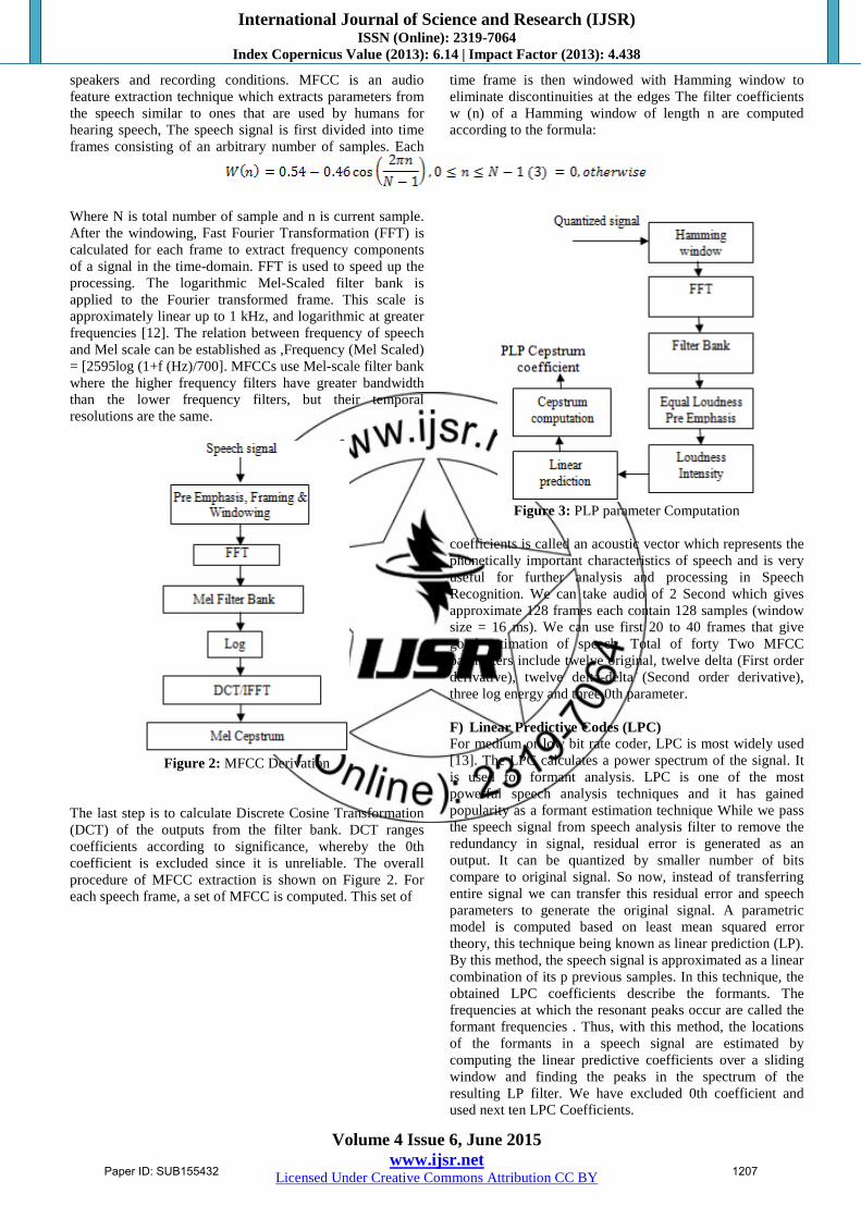
Figure 2: MFCC Derivation

The last step is to calculate Discrete Cosine Transformation

(DCT) of the outputs from the filter bank. DCT ranges

coefficients according to significance, whereby the 0th

coefficient is excluded since it is unreliable. The overall

procedure of MFCC extraction is shown on Figure 2. For

each speech frame, a set of MFCC is computed. This set of

Figure 3: PLP parameter Computation

coefficients is called an acoustic vector which represents the

phonetically important characteristics of speech and is very

useful for further analysis and processing in Speech

Recognition. We can take audio of 2 Second which gives

approximate 128 frames each contain 128 samples (window

size = 16 ms). We can use first 20 to 40 frames that give

good estimation of speech. Total of forty Two MFCC

parameters include twelve original, twelve delta (First order

derivative), twelve delta-delta (Second order derivative),

three log energy and three 0th parameter.

F) Linear Predictive Codes (LPC)

For medium or low bit rate coder, LPC is most widely used

[13]. The LPC calculates a power spectrum of the signal. It

is used for formant analysis. LPC is one of the most

powerful speech analysis techniques and it has gained

popularity as a formant estimation technique While we pass

the speech signal from speech analysis filter to remove the

redundancy in signal, residual error is generated as an

output. It can be quantized by smaller number of bits

compare to original signal. So now, instead of transferring

entire signal we can transfer this residual error and speech

parameters to generate the original signal. A parametric

model is computed based on least mean squared error

theory, this technique being known as linear prediction (LP).

By this method, the speech signal is approximated as a linear

combination of its p previous samples. In this technique, the

obtained LPC coefficients describe the formants. The

frequencies at which the resonant peaks occur are called the

formant frequencies . Thus, with this method, the locations

of the formants in a speech signal are estimated by

computing the linear predictive coefficients over a sliding

window and finding the peaks in the spectrum of the

resulting LP filter. We have excluded 0th coefficient and

used next ten LPC Coefficients.






G) Perceptual Linear prediction (PLP)

The Perceptual Linear Prediction PLP model developed by

Hermansky. PLP models the human speech based on the

concept of psychophysics of hearing. PLP discards irrelevant

information of the speech and thus improves speech

recognition rate. PLP is identical to LPC except that its

spectral characteristics have been transformed to match

characteristics of human auditory system

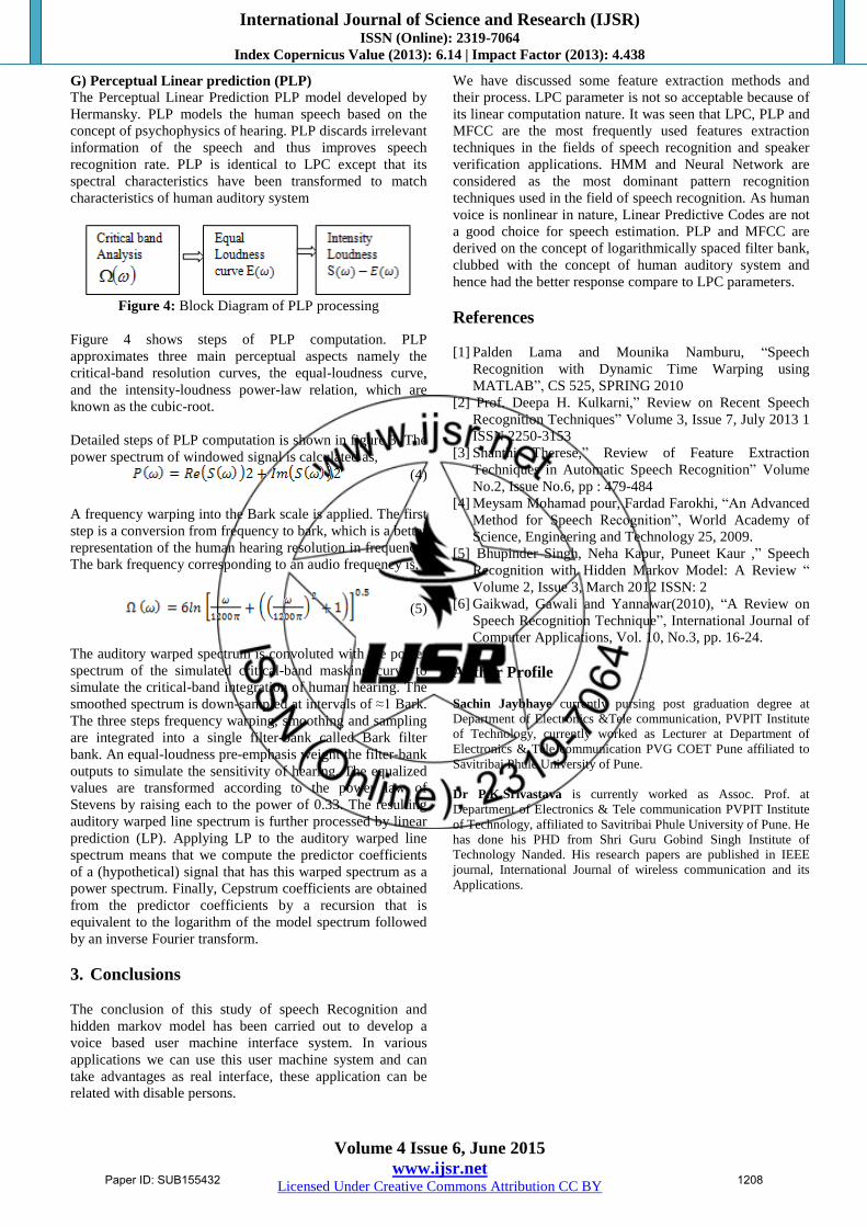
Figure 4: Block Diagram of PLP processing

Figure 4 shows steps of PLP computation. PLP

approximates three main perceptual aspects namely the

critical-band resolution curves, the equal-loudness curve,

and the intensity-loudness power-law relation, which are

known as the cubic-root.

Detailed steps of PLP computation is shown in figure 3. The

power spectrum of windowed signal is calculated as,

(4)

A frequency warping into the Bark scale is applied. The first

step is a conversion from frequency to bark, which is a better

representation of the human hearing resolution in frequency.

The bark frequency corresponding to an audio frequency is,

(5)

The auditory warped spectrum is convoluted with the power

spectrum of the simulated critical-band masking curve to

simulate the critical-band integration of human hearing. The

smoothed spectrum is down-sampled at intervals of ≈1 Bark.

The three steps frequency warping, smoothing and sampling

are integrated into a single filter-bank called Bark filter

bank. An equal-loudness pre-emphasis weight the filter-bank

outputs to simulate the sensitivity of hearing. The equalized

values are transformed according to the power law of

Stevens by raising each to the power of 0.33. The resulting

auditory warped line spectrum is further processed by linear

prediction (LP). Applying LP to the auditory warped line

spectrum means that we compute the predictor coefficients

of a (hypothetical) signal that has this warped spectrum as a

power spectrum. Finally, Cepstrum coefficients are obtained

from the predictor coefficients by a recursion that is

equivalent to the logarithm of the model spectrum followed

by an inverse Fourier transform.

3. Conclusions

The conclusion of this study of speech Recognition and

hidden markov model has been carried out to develop a

voice based user machine interface system. In various

applications we can use this user machine system and can

take advantages as real interface, these application can be

related with disable persons.

We have discussed some feature extraction methods and

their process. LPC parameter is not so acceptable because of

its linear computation nature. It was seen that LPC, PLP and

MFCC are the most frequently used features extraction

techniques in the fields of speech recognition and speaker

verification applications. HMM and Neural Network are

considered as the most dominant pattern recognition

techniques used in the field of speech recognition. As human

voice is nonlinear in nature, Linear Predictive Codes are not

a good choice for speech estimation. PLP and MFCC are

derived on the concept of logarithmically spaced filter bank,

clubbed with the concept of human auditory system and

hence had the better response compare to LPC parameters.

References

[1] Palden Lama and Mounika Namburu, “Speech

Recognition with Dynamic Time Warping using

MATLAB”, CS 525, SPRING 2010

[2] Prof. Deepa H. Kulkarni,” Review on Recent Speech

Recognition Techniques” Volume 3, Issue 7, July 2013 1

ISSN 2250-3153

[3] Shanthi Therese,” Review of Feature Extraction

Techniques in Automatic Speech Recognition” Volume

No.2, Issue No.6, pp : 479-484

[4] Meysam Mohamad pour, Fardad Farokhi, “An Advanced

Method for Speech Recognition”, World Academy of

Science, Engineering and Technology 25, 2009.

[5] Bhupinder Singh, Neha Kapur, Puneet Kaur ,” Speech

Recognition with Hidden Markov Model: A Review “

Volume 2, Issue 3, March 2012 ISSN: 2

[6] Gaikwad, Gawali and Yannawar(2010), “A Review on

Speech Recognition Technique”, International Journal of

Computer Applications, Vol. 10, No.3, pp. 16-24.

Author Profile

Sachin Jaybhaye currently pursing post graduation degree at

Department of Electronics &Tele communication, PVPIT Institute

of Technology, currently worked as Lecturer at Department of

Electronics & Tele communication PVG COET Pune affiliated to

Savitribai Phule University of Pune.

Dr P.K.Srivastava is currently worked as Assoc. Prof. at

Department of Electronics & Tele communication PVPIT Institute

of Technology, affiliated to Savitribai Phule University of Pune. He

has done his PHD from Shri Guru Gobind Singh Institute of

Technology Nanded. His research papers are published in IEEE

journal, International Journal of wireless communication and its

Applications.


review on speech recognition techniques · speech recognition, ... punjabi, hindi. b) dynamic time...

Documents