rethinking the rogowski model - nd.ntu.edu.t€¦ · international market and the scarcity factor...

2015 12 95-138

95

Rethinking the Rogowski Model: Taiwan’s Trade Policy and

Domestic Political Alignment 1996-2008*

Mark W. Lai**

2015 10 14 2015 11 3

* DOI:10.6164/JNDS.15-1.3 ** Associate Professor Department of International affairs Wenzao Ursuline University

of Languages. Expertise: International Political Economy, International Relations, Foreign Policy. B.A. in Philosophy, National Taiwan University. M.A. in Political Economy, New York University. Ph. D. in Political Science, State University of New York at Albany. E-mail: [email protected]

96

Abstract

The political economic relationship between Taiwan and China moved in a positive direction after the KMT returned to power in 2008. The launching of the Economic Cooperation Framework Agreement (ECFA) in September 2010 symbolized the prospect of economic and political reconciliation across the Taiwan Strait. Several years later, in light of the scholarly debate and waves of street protests by the opposition party and dissenters, it has become apparent that scholars ought to reexamine the validity of Rogowski’s model of trade policy and domestic political alignment, specifically with regard to its ability to explain the transformation of cross-strait political and economic interaction.

This study conducts an empirical analysis of the effects of economic liberalization on domestic political alignments and offers some hypotheses using updated data for testing. Highlighting certain policy implications with regard to disputes surrounding the ECFA issue, the study provides a new perspective for explaining cross-strait economic interaction and its implications for domestic politics.

Keywords: Rogowski Model, ECFA, Cross-Strait Relations, Trade Policy

Rethinking the Rogowski Model

97

The political economic relationship between Taiwan and China moved in a positive direction after the KMT returned to power in 2008. The launching of the Economic Cooperation Framework Agreement (ECFA) in September 2010 symbolized the prospect of economic and political reconciliation across the Taiwan Strait (Wei, 2010: 32-36). Several years later, in light of the scholarly debate and waves of street protests by the opposition party and dissenters, it has become apparent that scholars ought to reexamine the validity of Rogowski’s model of trade policy and domestic political alignment, specifically with regard to its ability to explain the transformation of cross-strait political and economic interaction.

Building on certain well-known economic theorems—such as those by Heckscher-Ohlin and Stolper-Samuelson—political scientist Ronald Rogowski offered a model that asserted that as a closed economy faces opening of international trade, the endowment factors inside the economy will shift: the abundant factor will be impacted positively from the international market and the scarcity factor will be impacted negatively because of competition created through liberalizing outside trade relations. Thus, the abundant factor tends to support political parties that welcome free trade, while the scarcity factor supports protectionism (Rogowski, 1989; Rogowski, 1987: 1121-1137; Rogowski, 1987: 203-223). In Taiwan’s case, the enormous increase of cross-strait economic interaction from 1989 to 2008 had established a strong interdependence and this case fits the close-to-open economy scenario. In this case, China, rather than the international market at large, has become the factor of liberalization. From the viewpoint of Rogowski’s model, the scarcity endowment in Taiwan, such as land and labor factors, has been impacted negatively, and therefore has tended to support an anti-China political position. The abundant capital factor has taken a pro-China stance (Keng and Chen, 2003: 1-29).

This study will reexamine this notion and conduct an empirical test

98

using three steps. First, previous research that has applied Rogowski’s model has explained Taiwan’s regional politics by proposing that the winners and losers in cross-strait economic relations could be discerned by a North-South political orientation. By contrast, this study suggests that the basic inferences of Rogowski’s model, along with Jefferey Frieden and Peter Trubowitz’s application to the Taiwan case (“RFT” Model), have logical and empirical problems. This study will show that with proper adjustments, the RFT model can generate better predictions for the Taiwan case. Second, scholars Paul Midford, Edward Leamer, Michael J. Hiscox and Jeffrey W. Ladewig, among others, have provided an alternative approach that can enrich the RFT model. Examining the arguments of these scholars, this study will further scrutinize the effect of economic liberalization on domestic political alignments. Third, this study will offer some hypotheses using updated data for testing. The time frame of this empirical study focuses on the years from 1996 to 2008 for three reasons. First, Taiwan did not have its first direct presidential election until 1996 and the results of the elections were the only direct and strong material for testing. Second, when the pro-China KMT political party returned to power in 2008, Taiwan’s industrial development and political alignment had entered a different phase. Both business and political sectors had accepted the necessity of integration with China while debating only the pace of integration. Compared with her former bosses- former presidents Lee Teng-hui and Chen Shui-bian- Tsai Ing-wen, the anti-China political DPP party’s presidential candidate in 2012 and 2016, has adopted a moderate and compromising attitude and policy toward China. Third, these facts made the years between 1996 and 2008 an interesting time period for researchers to study why under the great attraction of China’s money and even greater threat of China’s guns, Taiwanese still elected independence-leaning presidents who adopted anti-China policies.

In summary, this study will highlight certain policy implications with regard to disputes surrounding the ECFA issue and it will provide a new


99

perspective for explaining cross-strait economic interaction and its implications for domestic politics.

Finally, it should be noted that though the present study seeks to understand the possible connections between national trade policy and domestic political alignment and therefore focuses on cross-strait relations, the significant correlations between these two factors do not imply the exclusion of other important factors in explaining cross-strait relations, nor the denial of other important factors in determining domestic political alignment.

Literature Review: The RFT Model

Even as some scholars of international trade have downplayed the political effects and political reactions to the changing international commercial environment (Ellis et al., 1949; Corden, 1997), the early works of some political economists such as E. E. Schattschneider and Peter Gourevitch, have helped to establish research on the connection between special business interests and related political movements (Schattschneider, 1935; Gourevitch, 1986). Following this line of research, analyses of trade, economic policy and political developments in advanced economies have reached a significant critical mass worthy of summation (Yang, 1995: 956-963; Rankin, 2001: 351-376; Samuelson, 2004: 135-146; Baker, 2005: 924-938). However, the application of this line of analysis to the commercial and political context across the Taiwan Strait remains in the early stages. In 1999, Wu and Yen were among the first to use a statistical model to analyze the relationship between political influence and cross-strait commerce (Wu and Yen, 1999: 43-62; Wu and Yen, 2001: 135-166). Keng and Chen later argued that northern Taiwan benefits most from cross-strait economic interaction and therefore favors a pro-China political coalition while southern Taiwan tends toward an anti-China stance because its economy is concentrated in agriculture and labor-intensive

100

industries. Central Taiwan shows no significant trend in terms of its political alignment due to its mixed economy (Keng and Chen, 2003: 5). Lai’s doctoral dissertation established a statistical model explaining the correlation between Taiwan’s domestic political reforms and fluctuations in cross-strait hostilities (Lai, 2006). Keng & Chen’s and Lai’s research adopted theories from three sources: Ronald Rogowski’s theory in trade policy and domestic political alignment, Jefferey Frieden’s emphasis on globalization and investment, and Peter Trubowitz’s categorization of regional interests in analyzing foreign policy. Figure 1 below illustrates the inferences and synergy of these three theoretical models.

Figure 1: Rogowski, Frieden and Trubowitz’s (RFT) Models in Taiwan’s Case

Nevertheless, these three theoretical models share similar problems in their empirical modeling. First, Ronald Rogowski linked political alignment and free trade policy only under the simplified economic model and universal generalization was not his intention in developing the model (Rogowski, 1989:175-177). The excessive parsimony of a three-factor model makes it difficult to explain specific historical facts. For example, in Taiwan’s case, Rogowski’s model cannot explain why labor-intensive industries did not form effective political coalitions to promote a


101

protectionist policy toward Chinese imports. The reason for this was that under the long period of KMT authoritarianism, union organization in Taiwan was restricted to state-owned enterprises and a small number of KMT-backed conglomerates. When cross-strait commerce began to endanger local jobs and income, there was no consolidated labor union to act as a political counter-weight. 1 Moreover, for the Taiwan case, Rogowski’s model cannot explain why certain capital-intensive industries do not support a pro-China commercial policy. For example, pro-green companies have long supported government restrictions on Chinese imports.2 Such pro-green companies target different markets in the global economy and the further integration of the China-Taiwan market would create competition that would threaten their economic interests. In sum, Rogowski’s model oversimplified the factor of production and it sometimes fails to provide comprehensive explanations for specific historical cases.

Making allowances for Taiwan’s special economic relations with China (significant in both trade and investment), Keng and Chen applied Jeffrey Frieden’s theory concerning the politics of capital mobility under globalization. Frieden’s argument has two main dimensions. First, international financial integration tends to favor capital over labor/land because the former is easily movable, thus creating a significant advantage in a fast-paced international investment environment. In Taiwan’s case, after the enlargement of cross-strait commercial integration, the abundant capital factor became a favored investment target. On the other hand, the scarce labor and land factor proved difficult to move, and was not favored for investment in mainland China. The relative gain between the abundant

1 The total labor force in Taiwan is approximately 10 million people. The biggest labor

organization in Taiwan, Chinese Federation of Labor (CFL) has only 1.1 million members. Therefore, labor in Taiwan does not possess political influence proportionate to the size of the labor force. http://www.cfl.org.tw/page1.aspx?no= 100100125181730296.

2 Pro-green companies refer to businesses which support the DPP. They have generally

held an anti-China political stance.

102

factor and scarcity factor meant that capital became a beneficiary and labor/land became a victim of capital’s rise in importance. Combining the theoretical perspectives of Rogowski and Frieden indicates that the estimation of Taiwan’s economic restructuring must take into account not only what is traded across the Strait, but also what is invested.

On the other hand, as the second argument of Frieden’s investment theory notes, national investment policy is influenced by tensions such as those between internationally diversified and undiversified, tradable and non-tradable, and capital-mobile and. non-mobile divisions (Frieden, 1991:426). Frieden’s theory on international investment is modest and his evidence is limited. He calls for further empirical testing and the adaptation of the theory to different cases (Frieden, 1991:451). It should be noted that cross-strait investment differs from ordinary FDI or capital investment. It is better understood as akin to an enlargement of Taiwan’s market, widening to meet the Chinese market. While many industries, businesses and investors are trying to find long-term opportunities in China, cross-strait investment is more similar to the moving-out of economic resources. This moving out of resources has impacted Taiwan’s economy and has forced it to move to the next level of economic restructuring. The different industry preferences for mainland China investments and their political effects must be discerned through careful examination.

The research of Keng & Chen and Lai both support the Trubowitz model, which rests on a division of interests to explain differences in regional political alignments (Keng and Chen, 2003: 6-7; Trubowitz, 1998:4). Basically, according to the Trubowitz model, conflicts over national policies must be understood in the context of larger domestic struggles for regional economic advantage and political power (Trubowitz, 1998:6). Nevertheless, a problem with this model is that it does not account for whether a local region represents a unified economy, or whether certain constituents or political representatives would even


103

prioritize economic policy, as possibly revealed in their voting patterns. Certain scholars have raised doubts with regard to these issues and they have called for a more careful categorization of economic and political blocs (Fordham and McKeown, 2003: 520; Goff and Grier, 1993: 5-20).

In terms of the Taiwan case, the conventional understanding of regional politics has been based on a standard geographical division of North and South (Lee and Hsu, 2002: 61-84). Keng and Chen’s research has also adopted this approach, claiming that northern and southern Taiwan have opposing political stances while the central and eastern regions are neutral (Keng and Chen, 2003: 10, 15, 17). However, there remain certain anomalies that arise from these simplistic geographical divisions. For example, Taipei City and Taipei County are neighbors in northern Taiwan and thus should share similar socio-economic features. However, the city and county have different political cultures and voting preferences. For about half of the past two decades, the mayor of these two administrative units belonged to opposing political parties.3 With respect to southern Taiwan, the metropolitan city of Kaoshiung is relatively distinct compared to the agriculture-based counties surrounding it.4 Though differing in social-economic features, the voting preferences in the South are generally similar. These inconsistencies show the need for a more accurate way to discern political economic units when applying Trubowitz’s model to the Taiwan case. Table 1 summarizes and lists the major problems arising from applying the RFT model to the Taiwan case.

3 Appendix 1.

4 Differences in income, education, and other social-economic resources are apparent.

See Appendix.

104

Table 1: Propositions and Problems of RFT’s Theory in Taiwan case

Scholars Rogowski Frieden Trubowitz

Proposition Capital, labor and land form political coalition based on their loss or gain in international commerce

International capital investment is a very important factor in analyzing commercial policy and political reaction

Conflicts over national policies must be viewed in the context of larger domestic and regional struggles.

Problems Excessive parsimony in defining the factor endowments neglects the specifics of different economies.

The differences among capital investment, foreign direct investment, moving-out of industries and outsourcing are not stressed.

Simplistic geographical designations are only effective in regions with high homogeneity. Careful selection and definition of the geo units is necessary.

In Taiwan As an economy depending on foreign trade, most factors favor open trade policy

The nature of investment from Taiwan to China is the moving-out of industries. The corresponding political effect is complicated.

The simplistically defined North and South designations are problematic because the composition of the regions is not homogeneous.

In sum, the RFT model offers a generally correct prediction with regard to Taiwan’s political alignment under globalization and its changing national trade policy. However, a further refinement of the theoretical perspective is required and further empirical testing is also needed.

Research Design: The Modified RFT Model

Addressing the deficiencies noted above, Paul Midford and Edward Leamer have offered a similar but more sophisticated model. Paul Midford


105

has noted a major flaw in the Rogowski model: every economy has specific spatial-temporal conditions and thus requires more detailed categorical endowments. Unlike a simplified or primitive economy, an advanced economy with a democratic polity requires more sophisticated categorization that can address its size and complexity (Midford, 1993: 546). In the face of the liberalization of international trade, there are conflicts of interest between different elements of the capital factor in Taiwan: capital embedded in foreign trade will benefit from liberalization while capital exclusively embedded in domestic markets (e.g., in certain service sectors) will suffer because of more competition from inside and outside. Low-skilled labor is in favor of protectionist policy while high-skilled labor (e.g., management and white collar jobs) “can” support the opposite stance. Land with commercial usage will benefit from the economic growth brought by liberalization and the agricultural/industrial land will suffer from the import of cheaper food and products. These distinctions further clarifying the three major factors can help us better understand the aftermath of political alignments.

Leamer has provided an alternative model that features detailed factor endowments. He was one of the first economists to have noted the different effects of high innovation and low innovation industries newly exposed to international trade. His work addressed in greater detail the division of labor in each endowment and elaborated on how the factors have been established. He also innovatively employed the multi-factor model to examine possible combinations of over six factors (Leamer, 1984). For the Taiwan case, Leamer’s work can inspire the formulation of several combinations of factor endowments: labor-capital industry (e.g., Taiwan’s high-tech Science Parks), land and low-skilled labor (e.g., mining industry), domestic capital and high-skilled labor (e.g., financial sector) and others. The political stances of these combinations provide a counter-balance to the limited predictive capability of the Rogowski model.

106

In addition to addressing the factors of production found in the Leamer and Midford models, the present study also treats the important issues of mobility and conflict inside Taiwan’s economy, in particular, conflict between one factor and another, between one sector and another, or between employer and employee. For example, the abundant capital factor may not benefit from the liberalization of cross-strait commerce, despite what the Rogowski model suggests: immobile capital such as that found in the energy and petroleum industries would suffer from cheaper imports, employees in mobile capital-intensive industries would suffer, and the interests between mobile capital and immobile labor would clash and generate further political struggle. This type of more detailed analysis within the scope of production endowments would improve the application of the Rogowski model to the Taiwan case.

Since 1989 when cross-strait economic integration began to gradually increase and create a greater China economic sphere, the issue of mobility has increasingly been applicable to the domestic economy, which is affected by cross-strait commerce. A theory related to this issue, as stated by Michael J. Hiscox, says “if factors are mobile between industries, the income effects of trade divide individuals along class lines, setting owners of different factors (such as labor and capital) at odds with each other regardless of the industry in which they are employed. If factors are non-mobile between industries, the effects of trade can divide individuals along industry lines, setting owners of the same factor in different industries at odds with each other over policy (Hiscox, 2001: 2).” In other words, the industry with mobility is likely to increase competition among different endowments and the industry without mobility is likely to encourage rivalry between rich and poor. In Taiwan’s case, industries with high mobility can move out to mainland China to pursue higher profit and more expansion opportunities. This moving-out trend would give rise to political conflict among the factors of production (e.g., labor vs. capital, or more specifically, between laid-off workers and business owners who shift investments to China). On the other hand, industries with low mobility


107

might remain, but then face competition from imports, giving rise in turn to political conflict between rich and poor within the same endowment (e.g., between labor and owners of state-owned enterprises, and labor and owners of private heavy industries).

How will those who are impacted negatively and positively react to trade policy? Jeffrey W. Ladewig’s empirical tests support the proposition that globalization has dramatically brought mobility to industries. Thus, U.S. non-mobile industries have tried to influence Congressional politics to block the further integration of mobile international commerce (Ladewig, 2006: 69). By contrast, Gyung-Ho Jeong has examined the voting record of the U.S. Congress, showing that trade policy is defined by class-based politics, though the links between policies, political parties and political maneuvering are weak (Jeong, 2009: 519-540). More specific to the conflict issue, Gene Grossman’s model of Partially Mobile Capital underscores how factors of production can shift from sector to sector, and shows how mobility depends on the different adjustment costs and the margins created (Grossman, 1983: 1-17). This approach helps to reveal conflicts not only among the factors but also among the sectors. Moreover, the cost and benefit analysis from the perspectives of the industries can help to identify the winners and losers and their political stances with regard to national trade policy. Mark R. Brawley has distinguished the economic and political concerns of employers and employees, focusing on, “two results from trade policy—the employment effect, and the effect on the price of their output (Brawley, 1997: 640).” In other words, the cost benefit analysis encompasses the different concerns of both employees and employers in response to varying trade policies.

In summary, based on these theories, the issues generated by the enormous volume of cross-strait commerce should be examined and the complex connection among industries and factors has to be identified. The present study takes Taiwan as a case study and tests the theories reviewed above. Table 2 below illustrates various scholarly responses to the RFT

108

model.

In the table, the column entitled “Breakdown of Endowments” represents an elaboration of the Midford and Leamer models as applied to the Taiwan case. The capital, labor and land factors are further broken down into sub-categories based on the winner/gainer ratio. Capital Factor: Capital (C) refers to financial capital investment. High

technology (HTC) is capital-intensive high-technology industries. Traditional industry (TIC) refers to labor or land-intensive sectors.

Labor Factor: Professionals (PL) are workers with competitive skills, and many are self-employed or with stable job positions. Highly- skilled labor (HL) and Low-skilled labor (LL) work for HTC and TIC respectively.

Land Factor: High-profit land (HPL) located in urban areas and mostly utilized by the service sector. Low-profit land (LPL) is for agricultural and industrial use and is located in rural areas.

The middle-right section shows that when the factor of mobility was introduced to the picture (based on the theories of Hiscox and Ladewig), the relationships among sub-categories can be further identified. Mobile factors are C, PL; immobile factors are HTC, TIC, HL, LL, HPL, LPL.

Table 2: Modifying RFT Model

Scholars Proposition Research Design for Taiwan Case

Midford, Leamer

Specification of Factors Every economy has its spatial-temporal conditions and needs specific categorical endowments. The cross endowments combination such as labor-capital factor or new factor such as innovation can be adopted.

Breakdown of Endowments Capital Factor: Capital(C), High technology(HTC) and traditional industry(TIC) Labor Factor: Professional(PL), Highly-skilled labor(HL) and Low-skilled labor(LL) Land Factor: High profit land(HPL) and less profit land: industrial and agricultural(LPL)


109


Hiscox, Ladewig

Issue of Mobility A mobile industry is likely to generate rivalry among different endowments and a non-mobile industry is likely to generate rivalry between rich and poor.

Mobility in the Factor Endowments Mobility: C, PL. Rivalry among factors: C-PL Immobility: HTC, TIC, HL, LL, HPL, LPL. Rivalry among classes: HTC-TIC, HL-LL, HPL-LPL

Grossman, Brawley

Detecting Conflicts The degree of mobility depends on the different adjustment cost and the margin created. Therefore, there are conflicts between employer and employee, one factor and another, and one sector and another.

Complexity of Conflicts Mobility/Employer/Rich/Service Capital(C) Professional(PL) Delete HTC Immobility/Employee/Poor/IndAgri Traditional Industry(TIC) Highly and low skilled labor(HLLL) Low profit land(LPL) Delete HPL

Along the Factor Line: Capital clashes with Professionals. The latter earn their living by irreplaceable and competitive skills while the former depend on financial benefits. Although both easily adapt to the changing international commercial environment, there is tension between them.

Along the Class Line: HTC clashes with TIC because of disparity in income standards. HL – LL and HPL – LPL are rivals for the same reason.

With regard to the issue of mobility, the identification of rivalries differs from the original Rogowski model. For example, the capital factor would not necessarily conflict with the labor factor—this is because both would be negatively impacted by off-shoring of industries. The land and labor factors do not necessarily get along when they compete for public resources.

In the table, the bottom–right quadrant focuses on conflicts among

110

factors: for example, between the Mobility/Employer/Rich/Service group and the Immobile/Employee/Poor/IndAgri group. For the Taiwan case, the more visible and valid political rivalry is between people with capital investment (C) and professionals (PL) who favor economic integration with China and people in traditional industries (TIC), high and low skilled labor (HL, LL), and low profit land (LPL) who are against pro-China commercial policies.

Among the factors, HTC and HPL have not been included as rivals because they are between mobility and non-mobility, rich and poor; their political stance in trade policy will not be as comparatively significant.

The Empirical Test: Model Specification, Variables, Findings, and Discussion of Model Specification

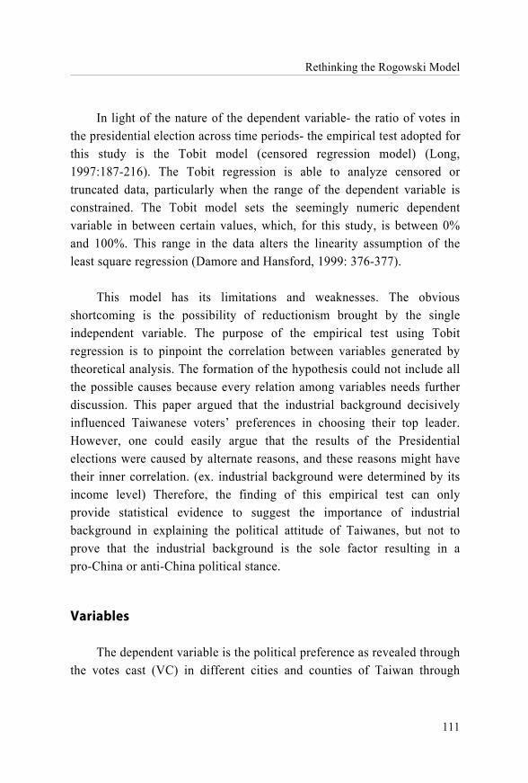
The empirical test in this study is intended to examine the possible correlation between industry differences in administrative units and their diverse political reactions. The dependent variable is the outcome Taiwan’s presidential election. Constituent voting behavior was influenced by independent variables generated from RFT and the new model, and controlled variables include education level, ethnic background, income level, age, political orientation of the administrative unit and the VC in the last time period (time series variable). The probability of more votes cast for an anti-China political coalition at a certain time point is VCt. As the value of VCt increases, the likelihood of more votes cast for an anti-China political coalition ought to increase. This process may be represented by:

t1t76

t5

t4

t3

t2

t1

t

e)VC(PO

AIETHEXVC


111

In light of the nature of the dependent variable- the ratio of votes in the presidential election across time periods- the empirical test adopted for this study is the Tobit model (censored regression model) (Long, 1997:187-216). The Tobit regression is able to analyze censored or truncated data, particularly when the range of the dependent variable is constrained. The Tobit model sets the seemingly numeric dependent variable in between certain values, which, for this study, is between 0% and 100%. This range in the data alters the linearity assumption of the least square regression (Damore and Hansford, 1999: 376-377).

This model has its limitations and weaknesses. The obvious shortcoming is the possibility of reductionism brought by the single independent variable. The purpose of the empirical test using Tobit regression is to pinpoint the correlation between variables generated by theoretical analysis. The formation of the hypothesis could not include all the possible causes because every relation among variables needs further discussion. This paper argued that the industrial background decisively influenced Taiwanese voters’ preferences in choosing their top leader. However, one could easily argue that the results of the Presidential elections were caused by alternate reasons, and these reasons might have their inner correlation. (ex. industrial background were determined by its income level) Therefore, the finding of this empirical test can only provide statistical evidence to suggest the importance of industrial background in explaining the political attitude of Taiwanes, but not to prove that the industrial background is the sole factor resulting in a pro-China or anti-China political stance.

Variables

The dependent variable is the political preference as revealed through the votes cast (VC) in different cities and counties of Taiwan through

112

time.5 The voting record was drawn from a national election which featured a host of national policy issues, and which directly involved cross-strait commercial policy issues. Due to the limited data, the left-hand side variable will be selected from different time periods to increase the sample size. The pool includes the presidential elections in 2000, 2004, and 2008.6 Since the China trade factor has played a crucial role in many of Taiwan’s national elections, these presidential elections represent the basic political preference of the Taiwanese people with regard to trade and commercial policies with China. In the appendix section, Chart 1 lists the descriptive statistic of this dependent variable. The ratio is the percentage of total votes for the anti-China political parties and coalition.7

The controlled variables are E (education), ETH (ethnicity), I (income), A (age), PO (political orientation of administrative unit) and (VC)t1 (political preference as revealed through election voting records through time/time series variable). Based on research on Taiwan’s electoral behavior, it is clear that these five variables can play significant roles in explaining election results (Wang, 2001: 95-123; Cheng, 2009: 23-49). In general, voters that support the anti-China DPP party have lower education levels, belong to the Taiwanese ethnic group, have lower income levels, and belong to a higher age group. Moreover, the political leaders of cities and counties can exert relatively significant power to influence presidential elections. The last variable is equivalent to the

5 There are 25 administrative units under the polity of Republic of China, Taiwan.

However, this research excluded the offshore islands of Quemoy and Matsu because of the large disparity of scale and institutional arrangement between these islands and the main island of Taiwan.

6 Limitation of data refers to the fact that Taiwan’s national statistics of all industries

across cities and counties is collected once in five years and the direct presidential election only began in 1996. The test has to be restrained by the limitation.

7 Candidates of the Democratic Progressive Party in these elections represented the

anti-China political coalition.


113

dependent variable, but it applies to past time periods. This is the controlled variable in the time series test. In the appendix section, Chart 2 shows the descriptive information pertaining to the control variables.

For the present study, the group of hypotheses and independent variables are drawn from Rogowski’s model (H1 and H2) and the modified model (H3, H4, and H5). This series of tests check the validity of RFT and modified models. The independent variables (explaining the outcome of the election) are as follows:

H 1 (SLR: Service Labor Ratio): The abundant capital factor is positively impacted by an open trade policy. The administrative units with a higher concentration of service sectors (based on capital investment and flow) are more likely to vote for a political coalition that supports an open trade policy toward China.

H 2 (ILR: Industry Labor Ratio, ALR: Agriculture Labor Ratio): The scarcity factors of labor and land are negatively impacted by an open trade policy. The units with higher concentration of industrial and agricultural sectors (relying on mass employment of labor and the usage of land) are more likely to vote for an anti-China coalition.

The test adopts as the operational variable the percentage of the population in industrial and agricultural sectors relative to the total population in the administrative unit. The population ratio, rather than the GDP ratio, has a direct relationship to the voting record. In the appendix section, Chart 3 illustrates the data for these three operational variables.

The second group of hypotheses and variables are drawn from the modified model:

114

H3 (MR: Manufacture Ratio, ALDR: Agriculture Land Ratio): The Immobility/Employee/Poor/IndAgri factors are negatively impacted by an open trade policy. The administrative units with a higher concentration of traditional industry (TIC), high and low skilled labor (HLLL) and low profit land (LPL) are more likely to vote for an anti-China political coalition. In this hypothesis, the operational variables are the MR, representing all the labor factors and traditional industry, and the ALDR, representing the cheap land variable.

H4 (PR: Professionals Ratio—population in financial sector, insurance companies, real estate and professional services sectors): Mobility/Employer/Rich/Service factors are positively impacted by an open trade policy. The administrative units with higher concentrations of C (Capital) and PL (Professionals) are more likely to vote for a pro-China political coalition. The PR variables both represent capital and professional factors.

In the appendix section, Chart 4 presents the data for these three operational variables.

The test was run six times with six sets of independent variables, plus five controlled variables and one time series variable.

Finding and Discussion

Below, Table 3 illustrates the study findings.


115

Table 3: Tobit Regression Analysis of Trade Policy and Domestic Political Alignment

Hypothesis H1 H2 H3 H4

Independent

Variables SLR ILR ALR MR ALDR PR

Coef. -0.264***

(0.087)

0.129

(0.085)

0.251*

(0.132)

0.127**

(0.051)

0.002***

(0.000)

-0.738*

(0.383)

Constant 0.352***

(0.069)

0.225***

(0.083)

0.233***

(0.076)

0.318***

(0.088)

0.250***

(0.068)

0.360***

(0.086)

Number of Obs 69 69 69 46 69 46

Log-likelihood 97.130 93.929 94.549 64.220 96.514 63.127

Pseudo R2 -0.666 -0.611 -0.622 -0.714 -0.655 -0.685

Dependent Variable: The ratio of votes for the anti-China political force in different administrative units Details of the empirical tests are in Appendix 1: Statistics Sheet *p<0.1, **p<0.05, ***p<0.01

The log likelihood of each of the models is large enough to reflect the observation numbers. The p values of the constant are all under 0.01. The models are in general a fit. The results of the Tobit analysis generally reflect the assertions of the hypotheses, although the level of significance varies. Thus, the study findings suggest two main points. First, hypotheses based on the RFT model (H1 and H2) show mixed results. The SLR (Service Labor Ratio) variable shows that counties and cities with higher service sector concentration tended to support a pro-China political coalition that would assure an open commercial policy toward China. With relatively less significance (p value less than 0.1), the ALR (Agriculture Labor Ratio) variable shows that counties and cities with higher agricultural sector concentration tend to support an anti-China political coalition. On the other hand, the ILR variable does not show enough significance in this test. The present study underscores the assertion that the different sectors inside the industry do make a difference in their overall political stance toward Taiwan’s trade policy. For example, high-skilled and low-skilled laborers have different preferences with

116

regard to national trade policy toward mainland China.

Moreover, the overall results of the new model (H3 and H4) show a consistent and strong correlation. The MR (Manufacture Ratio) variable represents the population of the manufacturing sector inside the industries. These are most likely to be negatively impacted by liberalized cross-strait commerce. The study findings indicate a notable significance (p value less than 0.05) in support of the hypothesis that cities and counties with higher manufacturing sector concentration are more likely to vote for an anti-China political coalition. The variable ALDR (Agriculture Land Ratio) shows a strong correlation (p value less than 0.01) between the negatively-impacted agricultural sectors and their antagonism toward an open trade policy with China; thus, the higher the percentage of agricultural land, the higher the tendency to vote for an anti-China political coalition. Finally, the variable PR shows a moderate significance (p value less than 0.1); cities and counties with higher concentrations of the professional class are less likely to vote for an anti-China political coalition.

In sum, the findings support the main argument of this paper. The RFT model indicates a good direction of possible correlation between Taiwan’s trade policy toward China and its domestic political alignment. Moreover, the new model generated by the present study provides more consistent theoretical inferences and more significant statistical results. Overall, in Taiwan, the administrative units with higher manufacturing and agricultural sector concentration and higher ratios of agricultural land tend to support an anti-China political coalition that holds a conservative attitude toward deepening cross-Strait commerce. And, administrative units with a higher service sector concentration and a larger population of professional workers will tend to support a political coalition that advocates an open trade policy with China.


117

Conclusion: Implications

With the impact of globalization, the relationship between trade and domestic politics is becoming increasingly complicated (Ocampo, 1998: 1523). Future research should examine the more complicated domestic realignments that result from the further integration of commercial relationships across borders.

Based on the findings of the empirical tests conducted, this study can shed light on at least one important policy implication. National trade policy has generated winners and losers in globalized economic competition. Citizens mobilize their political influence through interest groups, votes or street riots to alter the result of this global economic competition. Yet, this process can sometimes be destructive to the society at large. Clearly, cross-strait commerce impacts not only economic growth; it also impacts social, political, and economic inequality. Processes of political restructuring—and the ensuing social conflicts, protests, and upheavals they generate—arise in the wake of rapid economic transformation. Addressing these conflicts and smoothening economic development can be accomplished through public policy when it plays a constructive role in facilitating productive competition and when it protects innocent victims and consolidates a more open and plural society.

Paul Samuelson, the founding father of modern trade theory, Mancur Olson Jr., the renowned economist and political scientist, and Dani Rodrik, a well-regarded scholar of globalization, have all argued that the state should intervene to mitigate the negative impacts of free trade and improper trade, especially political confrontations between classes and sectors (Samuelson, 2004: 135-146; Olson, 1996: 3-24; Alesina and Rodrik: 1994, 465-490). Other researchers have noted how trade liberalization has brought overall poverty to politically unstable countries (Winters et al., 2004: 72). Research has suggested that a welfare system is

118

the remedy to the problem (Rudra, 2002: 411). Indeed, the present study underscores how national trade policies can reshapes domestic politics and engender political confrontation. Future research should focus on government policies with the aim of contributing to an understanding of how to alleviate the negative impacts of free trade policies.


119

Figure and Tables

Figure 1: Rogowski, Frieden and Trubowitz’s (RFT) Models in Taiwan’s Case

120

Table 1: Propositions and Problems of RFT’s Theory in Taiwan case

Scholars Rogowski Frieden Trubowitz

Proposition Capital, labor and land form political coalition based on their loss or gain in international commerce

International capital investment is a very important factor in analyzing commercial policy and political reaction

Conflicts over national policies must be viewed in the context of larger domestic and regional struggles.

Problems Excessive parsimony in defining the factor endowments neglect the specifics of different economies.

The differences among capital investment, foreign direct investment, moving-out of industries and outsourcing are not stressed.

Simplistic geographical designations are only effective in regions with high homogeneity. Careful selection and definition of the geo units is necessary.

In Taiwan As an economy depending on foreign trade, most factors favor open trade policy

The nature of investment from Taiwan to China is the moving-out of industries. The accordingly political effect is complicated.

The simplistically defined North and South designations are problematic because the composition of the regions is not homogeneous.


121

Table 2: Modifying RFT Model


Midford, Leamer

Specification of Factors Every economy has its spatial-temporal conditions and needs specific categorical endowments. The cross endowments combination such as labor-capital factor or new factor such as innovation can be adopted.

Breakdown of Endowments Capital Factor: Capital(C), High technology(HTC) and traditional industry(TIC) Labor Factor: Professional(PL), Highly-skilled labor(HL) and Low-skilled labor(LL) Land Factor: High profit land(HPL) and less profit land: industrial and agricultural(LPL)

Hiscox, Ladewig

Issue of Mobility A mobile industry is likely to generate rivalry among different endowments and a non-mobile industry is likely to generate rivalry between rich and poor.

Mobility in the Factor Endowments Mobility: C, PL. Rivalry among factors: C-PL Immobility: HTC, TIC, HL, LL, HPL, LPL. Rivalry among classes: HTC-TIC, HL-LL, HPL-LPL

Grossman, Brawley

Detecting Conflicts The degree of mobility depends on the different adjustment cost and the margin created. Therefore, there are conflicts between employer and employee, one factor and another, and one sector and another.

Complexity of Conflicts Mobility/Employer/Rich/Service Capital(C) Professional(PL) Delete HTC Immobility/Employee/Poor/IndAgri Traditional Industry(TIC) Highly and low skilled labor(HLLL) Low profit land(LPL) Delete HPL

122

Chart 1: Descriptive Statistics of the Voting Record

Unit and Year 1996 2000 2004 2008

Taipei 0.7083 0.3673 0.4694 0.3894

Yilan 0.8448 0.4703 0.5771 0.4858

Taoyuan 0.7101 0.3172 0.4468 0.3536

Hsinchu 0.7731 0.2475 0.3594 0.2598

Maioli 0.8057 0.2681 0.3925 0.2901

Taichung 0.7637 0.3651 0.5179 0.4116

Chunghua 0.8176 0.4005 0.5226 0.4241

Nantao 0.4814 0.3449 0.4875 0.3797

Yunlin 0.8546 0.4699 0.6032 0.5153

Chiayi 0.8864 0.4949 0.6279 0.5444

Tainan 0.8752 0.5378 0.6479 0.5615

Kasohsiung 0.8418 0.4714 0.584 0.5141

Pingtung 0.8838 0.4628 0.5811 0.5025

Taitung 0.818 0.232 0.3448 0.2668

Hualien 0.7529 0.2142 0.298 0.2252

Penghu 0.8253 0.3679 0.4947 0.4207

Keelung 0.6798 0.3084 0.4056 0.3227

Hsinchu City 0.6983 0.3379 0.4488 0.353

Taichung City 0.66 0.3686 0.4734 0.3826

Chiayi City 0.8039 0.4701 0.5606 0.4761

Tainan City 0.8043 0.4606 0.5777 0.4929

Taipei City 0.6324 0.3764 0.4347 0.3697

Kaohsiung City 0.7794 0.4579 0.5565 0.4841

* The ratio is the percentage of votes that DPP candidates gained in the presidential election. The ratio in 1996 is the combination of votes for KMT and DPP candidates because both parties adopted a strong anti-China stance in the campaign due to intense cross-Strait rivalry at the time caused by Beijing’s military exercises.

** The model will test 69 cases including 00, 04 and 08. The data for 1996 will be the control variable in the time-series model.

*** Source: Central Election Commission, Executive Yuan, ROC.


123

Chart 2: Descriptive Statistics of the Controlled Variables

Year and Unit E(00, 04, 08) ETH(00, 04, 08) I(00, 04, 08) A(00, 04, 08) PO(00, 04, 08)

Taipei 00 0.2342 0.752 251463 6.37 1

Yilan 00 0.1482 0.848 221787 10.2 1

Taoyuan 00 0.2063 0.517 253976 7.46 1

Hsinchu 00 0.2124 0.259 247438 9.69 1

Maioli 00 0.1492 0.336 201061 10.98 0

Taichung 00 0.187 0.742 208790 7.16 1

Chunghua 00 0.155 0.898 187578 9.42 0

Nantao 00 0.1611 0.829 196614 10.6 1

Yunlin 00 0.1374 0.921 221841 11.61 0

Chiayi 00 0.1248 0.851 205662 12.41 0

Tainan 00 0.172 0.918 200202 10.75 1

Kasohsiung 00 0.1663 0.791 197184 8.35 1

Pingtung 00 0.156 0.699 222350 10 1

Taitung 00 0.0856 0.488 202942 11.27 0

Hualien 00 0.1549 0.462 226182 10.73 0

Penghu 00 0.1898 0.879 228628 14.4 0

Keelung 00 0.2033 0.778 250981 8.81 1

Hsinchu City 00 0.2801 0.678 288539 8.46 1

Taichung City 00 0.3411 0.755 257604 6.49 1

Chiayi City 00 0.3243 0.819 233729 8.67 1

Tainan City 00 0.2913 0.864 234188 7.69 1

Taipei City 00 0.4232 0.679 338190 9.67 0

Kaohsiung City 00 0.2824 0.807 273281 7.16 1

Taipei 04 0.2886 0.752 258607 6.86 1

Yilan 04 0.2048 0.848 207785 11.54 1

Taoyuan 04 0.2608 0.517 260039 7.62 0

Hsinchu 04 0.2573 0.259 240242 10.58 0

Maioli 04 0.1958 0.336 202884 12.19 0

Taichung 04 0.2311 0.742 204780 7.9 0

Chunghua 04 0.201 0.898 206502 10.65 1

Nantao 04 0.2047 0.829 220406 11.96 1

Yunlin 04 0.1751 0.921 200515 13.26 0

Chiayi 04 0.1592 0.851 193479 13.98 1

Tainan 04 0.2123 0.918 208152 11.82 1

Kasohsiung 04 0.21 0.791 214761 9.16 1

Pingtung 04 0.1963 0.699 219940 11.13 1

Taitung 04 0.1241 0.488 203125 12.01 0

Hualien 04 0.2067 0.462 236692 11.41 0

124

Year and Unit E(00, 04, 08) ETH(00, 04, 08) I(00, 04, 08) A(00, 04, 08) PO(00, 04, 08)

Penghu 04 0.2303 0.879 229485 14.78 0

Keelung 04 0.2543 0.778 253161 9.71 0

Hsinchu City 04 0.3559 0.678 328112 8.81 0

Taichung City 04 0.4146 0.755 252330 7.15 0

Chiayi City 04 0.3954 0.819 223909 9.7 1

Tainan City 04 0.3511 0.864 240756 8.46 1

Taipei City 04 0.5013 0.679 380465 10.92 0

Kaohsiung City 04 0.3458 0.807 275576 8.24 1

Taipei 08 0.3472 0.735 285062 7.76 0

Yilan 08 0.2599 0.836 258516 12.83 0

Taoyuan 08 0.3183 0.56 271965 8.05 0

Hsinchu 08 0.3138 0.265 284478 11.2 0

Maioli 08 0.2474 0.367 219287 13.21 0

Taichung 08 0.2786 0.787 220907 8.68 0

Chunghua 08 0.2532 0.884 206670 11.79 0

Nantao 08 0.2504 0.797 212894 13.22 0

Yunlin 08 0.223 0.86 217561 14.73 1

Chiayi 08 0.2048 0.866 228268 15.35 1

Tainan 08 0.2603 0.884 222458 12.75 1

Kasohsiung 08 0.261 0.785 237839 10.11 1

Pingtung 08 0.2425 0.68 223284 12.26 1

Taitung 08 0.1699 0.527 196147 12.93 0

Hualien 08 0.2623 0.438 227134 12.26 0

Penghu 08 0.2734 0.806 244150 14.91 0

Keelung 08 0.3117 0.801 261760 10.77 0

Hsinchu City 08 0.4204 0.674 330721 9.29 0

Taichung City 08 0.4695 0.782 277705 7.92 0

Chiayi City 08 0.4544 0.823 247958 10.64 0

Tainan City 08 0.4027 0.873 273897 9.33 1

Taipei City 08 0.5719 0.694 386340 12.31 0

Kaohsiung City 08 0.4039 0.789 292349 9.57 1

* E refers to the ratio of citizens over the age of 15 with a college degree or above in different administrative units. ETH refers to Taiwanese (Hoklo) identification ratio (vs. Mainlander, Hakka or Aboriginal groups) in different administrative units. The survey was conducted in 2004 and 2008. Because there was no valid national survey data before 2004, the independent variables for 2000 will be substituted with those of 2004. I refers to the average income in each administrative unit. A is the ratio of the population above 65 years old in different administrative units. PO stands for political orientation and is represented by the mayors’ political party affiliation in the administrative unit—1 stands for an anti-China political coalition and 0 for the opposite.

** Sources: E: Department of Statistics, Ministry of The Interior, Executive Yuan, ROC. ETH: National Survey of Ethnic Groups in Taiwan, 2004, 2008, Council for Hakka Affairs, Executive Yuan ROC. I: Directorate General of Budget, Accounting and Statistics, Executive Yuan, ROC. A: Department of Statistics, Ministry of The Interior, Executive Yuan, ROC. PO: Central Election Commission, Executive Yuan, ROC.


125

Chart 3: Descriptive Statistics of H1 and H2

Unit and Year SLR(00, 04. 08) ILR(00, 04. 08) ALR(00, 04. 08)

Taipei 00 0.576 0.4107 0.0133

Yilan 00 0.5465 0.3623 0.0912

Taoyuan 00 0.4611 0.5063 0.0326

Hsinchu 00 0.4181 0.5308 0.0511

Maioli 00 0.4154 0.4756 0.109

Taichung 00 0.4279 0.4946 0.0775

Chunghua 00 0.3999 0.4477 0.1524

Nantao 00 0.485 0.3081 0.2069

Yunlin 00 0.4088 0.3382 0.2529

Chiayi 00 0.3789 0.3137 0.3074

Tainan 00 0.4212 0.4393 0.1394

Kasohsiung 00 0.4956 0.397 0.1073

Pingtung 00 0.4824 0.2883 0.2293

Taitung 00 0.4582 0.2606 0.2812

Hualien 00 0.6058 0.2643 0.13

Penghu 00 0.7448 0.1927 0.0626

Keelung 00 0.7031 0.2833 0.0136

Hsinchu City 00 0.539 0.4428 0.0182

Taichung City 00 0.713 0.2757 0.0113

Chiayi City 00 0.7027 0.2648 0.0325

Tainan City 00 0.5941 0.3846 0.0212

Taipei City 00 0.7886 0.2086 0.0027

Kaohsiung City 00 0.6653 0.3194 0.0153

Taipei 04 0.6142 0.3774 0.0084

Yilan 04 0.5665 0.3432 0.0902

Taoyuan 04 0.5058 0.4735 0.0207

Hsinchu 04 0.4735 0.4878 0.0387

Maioli 04 0.4587 0.4537 0.0876

Taichung 04 0.4705 0.4721 0.0574

Chunghua 04 0.4319 0.4498 0.1184

Nantao 04 0.5369 0.2624 0.2007

Yunlin 04 0.4601 0.3027 0.2372

Chiayi 04 0.4305 0.3008 0.2688

Tainan 04 0.4383 0.4281 0.1336

Kasohsiung 04 0.5144 0.3844 0.1012

Pingtung 04 0.5255 0.2693 0.2052

Taitung 04 0.5301 0.2204 0.2496

126

Unit and Year SLR(00, 04. 08) ILR(00, 04. 08) ALR(00, 04. 08)

Hualien 04 0.6478 0.2382 0.114

Penghu 04 0.735 0.1837 0.0813

Keelung 04 0.7064 0.2884 0.0053

Hsinchu City 04 0.5857 0.4032 0.0111

Taichung City 04 0.7234 0.2655 0.0112

Chiayi City 04 0.7521 0.2314 0.0165

Tainan City 04 0.6289 0.3511 0.02

Taipei City 04 0.8045 0.193 0.0025

Kaohsiung City 04 0.6778 0.3129 0.0093

Taipei 08 0.6168 0.3776 0.0056

Yilan 08 0.6017 0.3281 0.0703

Taoyuan 08 0.5131 0.4732 0.0137

Hsinchu 08 0.4652 0.5076 0.0272

Maioli 08 0.4766 0.4724 0.051

Taichung 08 0.4609 0.4958 0.0432

Chunghua 08 0.4249 0.4739 0.1012

Nantao 08 0.5228 0.2862 0.191

Yunlin 08 0.4578 0.3315 0.2107

Chiayi 08 0.4466 0.3469 0.2065

Tainan 08 0.4381 0.4608 0.1011

Kasohsiung 08 0.4982 0.4329 0.0689

Pingtung 08 0.5146 0.3144 0.171

Taitung 08 0.5492 0.2221 0.2287

Hualien 08 0.6578 0.2497 0.0925

Penghu 08 0.7131 0.2195 0.0674

Keelung 08 0.6925 0.3001 0.0074

Hsinchu City 08 0.5712 0.4214 0.0074

Taichung City 08 0.7002 0.2926 0.0073

Chiayi City 08 0.7196 0.269 0.0114

Tainan City 08 0.6003 0.3859 0.0138

Taipei City 08 0.8098 0.1879 0.0023

Kaohsiung City 08 0.684 0.3073 0.0087

* SLR refers to the ratio of the population in the service sector to the total population. ILR is the ratio of population in the industrial sector to the total population. ALR is the ratio of population in the agricultural sector to the total population.

** Source: Department of Statistics, Ministry of The Interior, Executive Yuan, ROC


127

Chart 4: Descriptive Statistics of H3 and H4

Unit and Year ALDR(00, 04. 08) Unit and Year MR(01, 06) PR(01, 06)

Taipei 00 16.71 Taipei 01 0.479588 0.047092

Yilan 00 12.94 Yilan 01 0.298063 0.055065

Taoyuan 00 32.87 Taoyuan 01 0.551441 0.037904

Hsinchu 00 21 Hsinchu 01 0.628642 0.029596

Maioli 00 19.27 Maioli 01 0.455147 0.045412

Taichung 00 25.78 Taichung 01 0.571492 0.044701

Chunghua 00 60.8 Chunghua 01 0.5649 0.04095

Nantao 00 16.02 Nantao 01 0.313759 0.053607

Yunlin 00 65.27 Yunlin 01 0.367189 0.051838

Chiayi 00 40.43 Chiayi 01 0.498781 0.030074

Tainan 00 46.62 Tainan 01 0.59458 0.03407

Kasohsiung 00 18.56 Kasohsiung 01 0.45702 0.044877

Pingtung 00 27.58 Pingtung 01 0.223631 0.063335

Taitung 00 13.57 Taitung 01 0.071941 0.077318

Hualien 00 9.93 Hualien 01 0.151403 0.076707

Penghu 00 43.65 Penghu 01 0.041326 0.066522

Keelung 00 5.57 Keelung 01 0.157746 0.054721

Hsinchu City 00 25.67 Hsinchu City 01 0.526828 0.060326

Taichung City 00 23.83 Taichung City 01 0.197538 0.18134

Chiayi City 00 42.48 Chiayi City 01 0.146857 0.106601

Tainan City 00 19.49 Tainan City 01 0.286881 0.086248

Taipei City 00 12.51 Taipei City 01 0.138176 0.160913

Kaohsiung City 00 5.96 Kaohsiung City 01 0.251535 0.097422

Taipei 04 16.55 Taipei 06 0.417386 0.061882

Yilan 04 12.76 Yilan 06 0.268284 0.057567

Taoyuan 04 31.83 Taoyuan 06 0.548579 0.043661

Hsinchu 04 20.81 Hsinchu 06 0.625583 0.036265

Maioli 04 18.82 Maioli 06 0.463409 0.044913

Taichung 04 24.59 Taichung 06 0.572926 0.030056

Chunghua 04 59.88 Chunghua 06 0.548266 0.041846

Nantao 04 16.24 Nantao 06 0.338101 0.051672

Yunlin 04 62.81 Yunlin 06 0.391818 0.053232

Chiayi 04 39.56 Chiayi 06 0.445385 0.03526

Tainan 04 46.04 Tainan 06 0.588213 0.034392

Kasohsiung 04 17.92 Kasohsiung 06 0.4457 0.036784

Pingtung 04 26.93 Pingtung 06 0.224159 0.06409

Taitung 04 13.57 Taitung 06 0.063555 0.068275

Hualien 04 10.01 Hualien 06 0.12229 0.074691

Penghu 04 45.53 Penghu 06 0.045301 0.062298

128

Unit and Year ALDR(00, 04. 08) Unit and Year MR(01, 06) PR(01, 06)

Keelung 04 5.54 Keelung 06 0.130274 0.054117

Hsinchu City 04 24.93 Hsinchu City 06 0.54177 0.057068

Taichung City 04 18.41 Taichung City 06 0.218965 0.112751

Chiayi City 04 42.22 Chiayi City 06 0.124083 0.107705

Tainan City 04 18.7 Tainan City 06 0.278128 0.087568

Taipei City 04 12.48 Taipei City 06 0.104973 0.203952

Kaohsiung City 04 3.67 Kaohsiung City 06 0.238721 0.089267

Taipei 08 15.46

Yilan 08 12.7

Taoyuan 08 30.66

Hsinchu 08 20.46

Maioli 08 18.66

Taichung 08 24.1

Chunghua 08 59.22

Nantao 08 16.01

Yunlin 08 62.6

Chiayi 08 39.09

Tainan 08 45.54

Kasohsiung 08 17.82

Pingtung 08 26.17

Taitung 08 13.66

Hualien 08 9.85

Penghu 08 44.78

Keelung 08 5.54

Hsinchu City 08 24.08

Taichung City 08 18.28

Chiayi City 08 34.5

Tainan City 08 18.16

Taipei City 08 12.18

Kaohsiung City 08 3.47

* ALDR refers to the ratio of agricultural land to total land. MR is the ratio of population in the manufacturing industrial sector to the total working population. PR is the ratio of population in the financial sector, insurance companies, real estate and professional services sectors to the total working population. The data of the latter two variables were only available in 2001 and 2006. Therefore, the empirical test adjusts to the sample number of 46, and the control and dependent variables shift to the years 2000 and 2004.

** Source: Department of Statistics, Ministry of The Interior, Executive Yuan, ROC, Directorate General of Budget, Accounting and Statistics, Executive Yuan, ROC


129

Table 3: Tobit Regression Analysis of Trade Policy and Domestic Political Alignment

Hypothesis H1 H2 H3 H4

Independent Variables

SLR ILR ALR MR ALDR PR

Coef. -0.264***(0.087)

0.129 (0.085)

0.251* (0.132)

0.127**(0.051)

0.002***(0.000)

-0.738* (0.383)

Constant 0.352***(0.069)

0.225*** (0.083)

0.233***(0.076)

0.318***(0.088)

0.250***(0.068)

0.360*** (0.086)

Number of Obs 69 69 69 46 69 46

Log-likelihood 97.130 93.929 94.549 64.220 96.514 63.127

Pseudo R2 -0.666 -0.611 -0.622 -0.714 -0.655 -0.685

Dependent Variable: The ratio of votes for the anti-China political party or coalition in different administrative units.

Details of the empirical tests is in Appendix 1: Statistics Sheet *p<0.1, **p<0.05, ***p<0.01

130

Appendix 1: Statistics Sheet

0 right-censored observations 69 uncensored observations Obs. summary: 0 left-censored observations /sigma .0592125 .0050405 .0491399 .0692852 _cons .3518271 .0685406 5.13 0.000 .2148597 .4887945 slr -.2641312 .0869607 -3.04 0.003 -.4379082 -.0903542 tr .4108102 .0474682 8.65 0.000 .3159527 .5056678 i -2.62e-07 3.24e-07 -0.81 0.421 -9.10e-07 3.85e-07 ed .2349847 .1465588 1.60 0.114 -.0578897 .5278592 po .0601017 .016047 3.75 0.000 .0280344 .092169 pvt1 -.1746077 .0450673 -3.87 0.000 -.2646675 -.0845478 pv Coef. Std. Err. t P>|t| [95% Conf. Interval]

Log likelihood = 97.130151 Pseudo R2 = -0.6659 Prob > chi2 = 0.0000 LR chi2(6) = 77.65Tobit regression Number of obs = 69

. tobit pv pvt1 po ed i tr slr, ll(0) ul(1)

0 right-censored observations 69 uncensored observations Obs. summary: 0 left-censored observations /sigma .0620239 .0052796 .0514735 .0725744 _cons .2253529 .0830212 2.71 0.009 .0594483 .3912575 ilr .1291181 .0852332 1.51 0.135 -.0412069 .2994431 tr .4086921 .0517193 7.90 0.000 .3053394 .5120448 i -3.75e-07 3.37e-07 -1.12 0.269 -1.05e-06 2.97e-07 ed .0847109 .14589 0.58 0.564 -.206827 .3762487 po .0593218 .0170819 3.47 0.001 .0251863 .0934572 pvt1 -.1723048 .0473766 -3.64 0.001 -.2669795 -.0776302 pv Coef. Std. Err. t P>|t| [95% Conf. Interval]


. tobit pv pvt1 po ed i tr ilr, ll(0) ul(1)


131

0 right-censored observations 69 uncensored observations Obs. summary: 0 left-censored observations /sigma .0614698 .0052327 .0510132 .0719264 _cons .2337059 .0757542 3.09 0.003 .0823231 .3850887 alr .2506038 .1323383 1.89 0.063 -.0138533 .5150608 tr .3586379 .0499461 7.18 0.000 .2588286 .4584472 i -3.97e-07 3.32e-07 -1.20 0.236 -1.06e-06 2.66e-07 ed .2478633 .1654505 1.50 0.139 -.0827631 .5784896 po .07031 .0168765 4.17 0.000 .0365851 .1040349 pvt1 -.1581687 .0467536 -3.38 0.001 -.2515983 -.064739 pv Coef. Std. Err. t P>|t| [95% Conf. Interval]


. tobit pv pvt1 po ed i tr alr, ll(0) ul(1)

0 right-censored observations 69 uncensored observations Obs. summary: 0 left-censored observations /sigma .0597434 .0050856 .0495807 .0699062 _cons .2499768 .0684636 3.65 0.001 .1131633 .3867903 ALDR .0015277 .0005456 2.80 0.007 .0004375 .0026179 tr .3290221 .0507069 6.49 0.000 .2276924 .4303518 i -2.19e-07 3.31e-07 -0.66 0.511 -8.80e-07 4.43e-07 ed .0829941 .1404394 0.59 0.557 -.1976516 .3636398 po .0759822 .0166419 4.57 0.000 .042726 .1092384 pvt1 -.1844778 .0459165 -4.02 0.000 -.2762346 -.092721 pv Coef. Std. Err. t P>|t| [95% Conf. Interval]


. tobit pv pvt1 po ed i tr ALDR, ll(0) ul(1)

132

0 right-censored observations 46 uncensored observations Obs. summary: 0 left-censored observations /sigma .0599023 .0062452 .0472803 .0725244 _cons .3181449 .0881421 3.61 0.001 .1400031 .4962867 MR1 .1268717 .0512213 2.48 0.018 .0233495 .2303939 PO1 .0186735 .0202703 0.92 0.362 -.0222944 .0596414 TIR1 .3975663 .0556462 7.14 0.000 .285101 .5100315 INC1 -8.70e-07 4.04e-07 -2.15 0.038 -1.69e-06 -5.28e-08 ED1 .3655027 .1862668 1.96 0.057 -.0109566 .741962 PVT1 -.1731644 .0477935 -3.62 0.001 -.2697587 -.0765701 PV1 Coef. Std. Err. t P>|t| [95% Conf. Interval]


. tobit PV1 PVT1 ED1 INC1 TIR1 PO1 MR1, ll(0) ul(1)

0 right-censored observations 46 uncensored observations Obs. summary: 0 left-censored observations /sigma .0613442 .0063945 .0484204 .074268 _cons .3604524 .0863986 4.17 0.000 .1858343 .5350705 PR1 -.7378035 .3828621 -1.93 0.061 -1.511597 .0359898 PO1 .0211402 .0207267 1.02 0.314 -.0207501 .0630305 TIR1 .3762184 .0561687 6.70 0.000 .2626971 .4897396 INC1 -8.63e-07 4.15e-07 -2.08 0.044 -1.70e-06 -2.52e-08 ED1 .5590403 .2249769 2.48 0.017 .104345 1.013736 PVT1 -.1433787 .0515233 -2.78 0.008 -.2475113 -.0392462 PV1 Coef. Std. Err. t P>|t| [95% Conf. Interval]


. tobit PV1 PVT1 ED1 INC1 TIR1 PO1 PR1, ll(0) ul(1)


133

Bibliography

Chinese-language sources

2003

42(6): 1-27

2010 ECFA

235: 32-36

1999

38(7): 43-62

2001

10(2): 135-166

English-language sources

Alesina, Alberto and Dani Rodrik (1994). “Distributive Politics and Economic Growth.” The Quarterly Journal of Economics 109(2): 465-490.

Baker, Andy (2005). “Who Wants to Globalize? Consumer Tastes and Labor Markets in a Theory of Trade Policy Beliefs.” American Journal of Political Science 49(4): 924-938.

Brawley, Mark R. (1997). “Factoral or Sectoral Conflict? Partially Mobile Factors and the Politics of Trade in Imperial Germany.” International Studies Quarterly 41(4): 640.

Cheng, Su-Feng (2009). “Ethnicity, Identity, and Vote Choice in Taiwan.” Journal of Electoral Studies 16(2): 23-49.

Corden, W. Max (1997). Trade Policy and Economic Welfare. New York: Oxford University Press.Ellis, Howard S. eds. (1949). Readings in the Theory of International Tread. York, PA: The Blakiston Company.

134

Damore, David F., Thomas G. Hansford, and A.J. Barghothi (2010). “Explaining the Decision to Withdraw from a U.S. Presidential Nomination Campaign.” Political Behavior 32(2):157-180.

Fordham, Benjamin, and Timothy J. McKeown (2003). “Selection and Influence: Interest Groups and Congressional Voting on Trade Policy.” International Organization 57(3): 520.

Frieden, Jeffrey A. (1991). “Invested Interests: The Politics of National Economic Policies in a World of Global Finance.” International Organization 45(4): 426, 451.

Goff, Brian L., and Kevin B. Grier (1993). “On the (Mis) Measurement of Legislator Ideology and Shirking.” Public Choice 76(1-2): 5-20.

Gourevitch, Peter (1986). Politics in Hard Times: Comparative Responses to International Economic Crises. Ithaca, N.Y.: Cornell University Press.

Grossman, Gene (1983). “Partially Mobile Capital: A General Approach to Two-Sector Trade Theory.” Journal of International Economics 15:1-17.

Hiscox, Michael J. (2001). “Class versus Industry Cleavages: Inter-Industry Factor Mobility and the Politics of Trade.” International Organization 55(1): 2.

Jeong, Gyung-Ho (2009). “Constituent Influence on International Trade Policy in the United States.” International Studies Quarterly 53: 519-540.

Ladewig, Jeffrey W. (2006). “Domestic Influences on International Trade Policy: Factor Mobility in the United States, 1963 to 1992.” International Organization 60(1): 69.

Lai, Wenyi M. (2006). “The economic and political sources of hostility: Taiwanese and Chinese relations, 1975 to 2004” PhD Diss., State University of New York at Albany.

Leamer, Edward (1984). Source of International Comparative Advantage: Theory and Evidence. Cambridge, Mass.: MIT Press.

Lee, Pei-Shan, and Yung-Ming Hsu (2002). “Southern Politics?


135

Regional Trajectories of Party Development in Taiwan.” Issues & Studies 38(2): 61-84.

Long, J. Scott (1997). Regression Models for Categorical and Limited Dependent Variables, Ch. 7 Limited Outcomes. The Tobit Model.London: Sage Publications

Midford, Paul (1993). “International Trade and Domestic Politics: Improving on Rogowski’s Model of Political Alignments.” International Organization 47(4): 542, 546

Ocampo, Jose Antonio (1998). “Trade Liberalisation in Developing Economies: Most Benefits but Problems with Productivity Growth, Macro Prices, and Income Distribution.” The Economic Journal 108(450): 1523.

Olson Jr. Mancur (1996). “Distinguished Lecture on Economics in Government: Big Bills Left on the Sidewalk: Why Some Nations are Rich, and Others Poor.” The Journal of Economic Perspectives 10(2): 3-24.

Rankin, David M. (2001). “Identities, Interests, and Imports.” Political Behavior 23(4): 351-376.

Rogowski, Ronald (1987). “Political Cleavages and Changing Exposure to Trade.” The American Political Science Review 81(4):1121-1137.

Rogowski, Ronald (1987). “Trade and the Variety of Democratic Institutions.” International Organization 41(2): 203-223.

Rogowski, Ronald (1989). Commerce and Coalitions: How Trade Affects Domestic Political Alignments. New Jersey: Princeton University Press.

Rudra, Nita (2002). “Globalization and the Decline of the Welfare State in Less-Developed Countries.” International Organization 56(2): 411.

Samuelson, Paul A. (2004). “Where Ricardo and Mill Rebut and Confirm Arguments of Mainstream Economists.” The Journal of Economic Perspectives 18(3): 135-146.

Schattschneider, E. E. (1935). Politics, Pressures, and the Tariff.

136

Englewood Cliffs, N.J.: Prentice Hall. Trubowitz, Peter (1998). Defining the National Interest: Conflict and

Change in American Foreign Policy. Chicago: The University of Chicago Press.

Wang, Ding-ming (2001). “The Impacts of Policy Issues on Voting Behavior in Taiwan: A Mixed Logit Approach.” Journal of Electoral Studies 8(2): 95-123.

Winters, Alan, Neil McCulloch and Andrew McKay (2004). “Trade Liberalization and Poverty: The Evidence so Far.” Journal of Economic Literature 42(1): 72.

Yang, C.C. (1995). “Endogenous Tariff Formation under Representative Democracy: A Probabilistic Voting Model.” The American Economic Review 85(4): 956-963.


137

1996-2008

*

2008 2010

* E-mail: [email protected]

rethinking the rogowski model - nd.ntu.edu.t€¦ · international market and the scarcity factor...

Documents