Responsiveness and Election Proximity in the United

States Senate

Christopher Warshaw⇤†

Department of Political ScienceMassachusetts Institute of Technology

This Draft: May 2016First Draft: February 2013

Abstract: One of the most important questions in the study of democratic representation iswhether elected o�cials are responsive to the preferences of their constituents, and whetherresponsiveness varies across institutional conditions. However, previous work on this questionhas been hampered by the unavailability of time-varying data on public opinion in eachconstituency. In this paper, I use new estimates of public opinion in each state-year from1950-2012 to examine whether Senators are responsive to changes in public opinion andwhether their behavior shifts over the course of the electoral cycle. I find that Senators aremodestly responsive to changes in public opinion. They are particularly responsive to publicopinion in the last two years of their term. But the impact of public opinion on Senators’ rollcall behavior is still small relative to the impact of electoral selection. This analysis resolvesearlier ambiguities in the literature on election proximity in the Senate, and opens up newresearch paths in the study of representation.

⇤Assistant Professor, Department of Political Science, Massachusetts Institute of Technology, cwar-shaw@mit.edu

†I am grateful to MIT’s School of Humanities, Arts and Social Sciences for research support. I thankparticipants in Columbia University’s Conference on Representation for very helpful feedback. I also thankAdam Berinsky, David Brady, Devin Caughey, Robert Erikson, Simon Jackman, Jonathan Rodden, ChrisTausanovitch, Emily Thorson, and Barry Weingast for their insightful comments on earlier version. Finally, Iam grateful to Stephen Brown, Jackie Han, and Melissa Meek for valuable research assistance. All mistakes,however, are my own.

1

One of the most important questions in the study of democratic representation is whether

elected o�cials are responsive to the preferences of their constituents. There are strong the-

oretical reasons to believe that legislators should be responsive to their constituents in order

to enhance their re-election prospects (Downs, 1957; Mayhew, 1974; Arnold, 1992). They

should be particularly responsive to changes in constituent preferences (Stimson, MacKuen,

and Erikson, 1995). Moreover, there are a variety of reasons to believe that legislators should

be most responsive to public opinion toward the end of the electoral cycle. Most importantly,

voters tend to overweight recent events (Achen and Bartels, 2004; Huber, Hill, and Lenz,

2012; Healy and Lenz, 2014). This is likely to incentivize politicians to consider the views of

their constituents more as elections grow more proximate.

There is a clear consensus among scholars that more liberal constituencies tend to elect

legislators that take liberal roll call positions (Miller and Stokes, 1963; Erikson and Wright,

2000; Ansolabehere, Snyder, and Stewart, 2001; Clinton, 2006). However, there is an active

debate about whether legislators respond to changes in the preferences in their constituents.

One set of studies finds no evidence that legislators shift their roll call behavior (Poole

and Rosenthal, 2000; Lee, Moretti, and Butler, 2004; Krimmel, Lax, and Phillips, 2015).

Rather, they “die in their ideological boots” (Poole, 2007, 435). Another set of studies finds

some evidence of movement in response to large, exogenous shifts in constituency opinion,

such as redistricting (Stratmann, 2000), variation in turnout due to rainfall (Henderson and

Brooks, Forthcoming), moves between chambers (Miler, Forthcoming), or during statewide

crises (Kousser, Lewis, and Masket, 2007). However, previous research on responsiveness

has been hampered by the lack of time-varying measures of citizens’ policy preferences in

1

each constituency.1 Only with time-varying measures is it possible to trace out the dynamic

process of responsiveness and identify how legislators respond to changes in public opinion.

A number of previous studies have examined how senators’ roll call behavior shifts over

the electoral cycle. These studies have found that Senators become more moderate as elec-

tions approach, presumably because they are shifting their behavior toward the median voter

in their state (Albouy, 2011; Amacher and Boyes, 1978; Elling, 1982; Lindstadt and Van-

der Wielen, 2011; Thomas, 1985; Wright and Berkman, 1986).2 But these studies too su↵er

from the “lack ... [of] a measure that taps actual constituency views against which to com-

pare senatorial voting records” (Ahuja, 1994). The unavailability of time-varying measures of

public opinion in each state has forced most previous studies to focus on the average change

in roll call behavior over the electoral cycle without reference to a measure of constituency

preferences. The previous studies on how responsiveness to public opinion varies over the

electoral cycle use cross-sectional data from just one or two election cycles, and thus lack a

credible causal identification strategy (Ahuja, 1994; Shapiro et al., 1990).

In this paper, I use new data and statistical techniques to examine democratic respon-

siveness and election proximity in the United States Senate. First, I examine dynamic

responsiveness using new estimates of citizen policy conservatism for each state and year

that are derived from the survey responses of over 700,000 individuals between 1950 and

2012. To summarize this large body of opinion data, I estimate a dynamic group-level item-

response model, producing yearly estimates of the average economic policy conservatism of

1 Only three previous studies have examined whether senators respond to changes in constituent prefer-ences (Levitt, 1996; Wood and Andersson, 1998; Buttice and Highton, Forthcoming). However, each of thesestudies uses proxies for constituent preferences rather than direct measure of public opinion.

2 In a related study, Huber and Gordon (2004) find that elected judges change their behavior in criminalsentencing cases as their reelection approaches.

2

the citizens of each state (Caughey and Warshaw, 2015). To measure legislators’ roll call

behavior, I use two di↵erent dynamic ideal point models to estimate how Senators’ ideal

points change over time (Martin and Quinn, 2002; Nokken and Poole, 2004). With these

new data in hand, I test whether Senators are responsive to changes in the views of their

constituents. I find that Senators are modestly responsive to shifts in public opinion: when

the state public moves to the left, Senators takes more liberal roll call positions. Moreover,

Senators are substantially more responsive to public opinion in the last two years of their

term than in the first four years of their term.

As a robustness check for my primary results, I also examine how the association between

senators’ roll call votes and public opinion on individual issues changes over the course of

the electoral cycle. This approach follows that of studies such as Gilens (2005), Lax and

Phillips (2009a), Matsusaka (2010), and Krimmel, Lax, and Phillips (2015). One benefit

of focusing on the link between individual roll call votes and issue-specific public opinion

is that this approach makes fewer assumptions about the dimensionality of the roll call

agenda and the public’s policy preferences (Broockman, 2016).3 It also makes it possible

to compare public opinion and roll call votes on the same scale (Lax and Phillips, 2009a;

Matsusaka, 2010). I examine the association between Senators’ roll call votes and public

opinion on individual issues by using multilevel regression with post-stratification (MRP)

models to estimate issue-specific public opinion on 72 individual policies, and then linking

public opinion on each policy directly to senators’ roll call votes. This analysis also indicates

that there is a much stronger association between Senators’ roll call votes and public opinion

3 However, while this approach is well-suited for examining how the association between public opinionand roll call behavior varies over the electoral cycle, it is not suitable for causally identifying the degree ofSenators’ responsiveness to public opinion.

3

in the last two years of their term.

Overall, my results establish a clear link between public opinion and senators’ roll call

votes. Moreover, legislators are most responsive to their constituents toward the end of the

electoral cycle. However, a one standard deviation change in citizen policy conservatism

corresponds to only a 0.02 standard deviation change in Senators’ roll call behavior. Even

in the last two years of senators’ term, a one standard deviation change in citizen policy

conservatism only corresponds to roughly a 0.04 standard deviation change in their roll call

behavior. So it is true that senators are responsive to changes in public opinion, and more

responsive in the last two years of their term, but the aggregate e↵ect of public opinion is

still small.

This paper proceeds as follows. First, I describe previous work on the e↵ect of public

opinion and election proximity on representation in the Senate, and describe my theory and

hypotheses. Then, I describe my research design for measuring dynamic responsiveness.

Next, I describe my main findings. Then, I check the robustness of my results using data

about public opinion and roll call votes on individual issues. Finally, I briefly conclude and

discuss the implications of my findings for our understanding of democratic representation

in Congress.

Dynamic Responsiveness

The central assumption of American legislative scholarship over the last 30 years is that

legislators are predominately, if not single-mindedly, motivated by electoral incentives (May-

hew, 1974; Kousser, Lewis, and Masket, 2007). Legislators’ re-elections hopes are likely to

4

be bolstered by adapting their positions to respond to changes in the opinion of their con-

stituents. Thus, “when politicians perceive public opinion change, they adapt their behavior

to please their constituency, and, accordingly, enhance their chances of reelection” (Stimson,

MacKuen, and Erikson, 1995, 545).

There is a broad array of evidence that citizens are capable of holding their legislators ac-

countable for their roll call behavior. Using survey data from the 1988-1992 Senate Election

Study, Ensley (2007) shows that the ideological divergence between Senate candidates influ-

ences citizens’ vote choices. Moreover, Ansolabehere and Jones (2010), Jessee (2009), and

Shor and Rogowski (2013) find that the extent to which a constituent agrees with the pol-

icy positions of their legislator a↵ects the constituent’s likelihood of voting for the member.

Looking at electoral results, there is also a wide array of empirical evidence that ideologi-

cally extreme legislators are penalized at the ballot box (Ansolabehere, Snyder, and Stewart,

2001; Canes-Wrone, Brady, and Cogan, 2002; Hall, 2015). This leads to the prediction that

legislators should be attentive and responsive to changes in the policy preferences of their

constituents.

However, several factors may dampen the incentives for legislators to be highly responsive

to changes in the views of their constituents. First, the re-election incentives for legislators

to respond to changes in public opinion actually appear to be surprisingly modest, possibly

because many voters have only a dim awareness of legislators’ roll call positions. Indeed,

Canes-Wrone, Brady, and Cogan (2002) finds that a one standard deviation moderation in

legislators’ roll call behavior only leads to a 2% increase in legislators’ vote shares. Sec-

ond, voters appear to punish candidates that reposition their views on individual issues

(Van Houweling and Tomz, 2011). This could reduce candidates’ incentives to respond to

5

changes in constituent opinion on individual issues.

There is a clear consensus among scholars that more liberal states are more likely to

elect senators that take liberal roll call positions (Erikson and Wright, 2000; Ansolabehere,

Snyder, and Stewart, 2001; Clinton, 2006). However, there is no consensus about whether

senators respond to changes in the public’s policy preferences in their state. Some studies

find little or no evidence of dynamic responsiveness. For instance, Poole (2007, 435) finds

that legislators do not change their positions over the course of their careers and thus “die

in their ideological boots.” Along these lines, Krimmel, Lax, and Phillips (2015) finds no

evidence that senators change their positions on gay rights in response to changes in their

constituents views.

In contrast, several other studies find evidence of modest dynamic responsiveness in the

Senate. Miler (Forthcoming) finds that newly elected senators that had previously served in

the House shift their positions toward the statewide median voter. Also, Buttice and Highton

(Forthcoming) finds that senators shift their positions in response to changes in presidential

voting patterns in their state. However, the implications of this study are unclear because

presidential vote shares may not clearly reflect public opinion in earlier eras, especially in

the one party south (Levendusky, Pope, and Jackman, 2008; Caughey and Warshaw, 2015).

So it’s unclear whether Buttice and Highton (Forthcoming) are observing responsiveness to

changes in public opinion, partisanship, voting behavior, or some other latent quantity.

6

Changes in Responsiveness Over the Electoral Cycle

There are strong theoretical reasons to believe that Senators’ political incentives change

over the course of the electoral cycle. Most importantly, a variety of observational studies

have found that voters overweight recent events when they evaluate incumbents’ performance

(e.g., Achen and Bartels, 2004). Several experimental studies have also found strong evidence

that voters overweight recent economic performance (Huber, Hill, and Lenz, 2012; Healy and

Lenz, 2014). For instance, Healy and Lenz (2014) find that voters focus on the election-year

economy because it is more accessible than information about the economy across the entire

electoral cycle. They suggest that this “reflects a general tendency for people to simplify

retrospective assessments by substituting conditions at the end for the whole.”

This tendency to overweight recent events is likely to be even stronger for assessments

of legislators’ roll call voting behavior than for the economy due to voters’ general lack

of information on legislators’ roll call positions. Franklin (1993) finds that respondents to

the 1988-1992 Senate Election Study were more likely to be able to place legislators on an

ideological scale in the last two years of their term.

Voters’ tendency to overweight recent events may give legislators freedom to take un-

popular positions early in their terms. In addition, it is likely to incentivize politicians to

consider the views of their constituents more as elections grow more proximate. Indeed,

a variety of qualitative evidence indicates that Senators have a general heuristic that they

should focus more on public opinion in the last two years of their term. For example, one

18-year Senate veteran told Richard Fenno: “My life [as a Senator] has a six-year cycle to

it... I say in the Senate that I spend four years as a statesman and two years as a politician.

7

You should get cracking as soon as the last two years open up. You should take a poll on

the issues, identify people to run my campaign in di↵erent parts of the state, raise money,

start my PR, and so forth” (Fenno, 1982, 29).

While there is little existing evidence about how responsiveness changes over the elec-

toral cycle, previous studies have found that Senators moderate their roll call behavior as

elections approach, presumably because they are shifting their behavior toward the median

voter in their state (Albouy, 2011; Amacher and Boyes, 1978; Elling, 1982; Lindstadt and

Vander Wielen, 2011; Thomas, 1985). These studies show that Democrats tend to shift to

the right in the last two years of their term, while Republicans tend to shift to the left.

Research Design

I examine dynamic responsiveness in the United States Senate using new estimates of citizen

policy conservatism for each state and year that are derived from the survey responses of

approximately 730,000 individuals to over 150 domestic policy questions fielded between 1950

and 2012 (Caughey and Warshaw, 2015). I also estimate a dynamic ideal point model to

estimate how Senators’ ideal points change over time (Martin and Quinn, 2002). With these

new data in hand, I can test whether Senators are responsive to changes in the views of

their constituents using a time-series cross-sectional (TSCS) approach, which enables me to

exploit within-legislator variation in public opinion and roll call behavior. Moreover, I can

examine how Senators’ roll call behavior changes over the course of the electoral cycle.

8

Citizen Policy Conservatism: 1950-2012

I follow Erikson, Wright, and McIver (1993), Stimson, MacKuen, and Erikson (1995), and

many others, in summarizing public opinion on a single dimension, which I label citizen eco-

nomic policy conservatism to distinguish it from ideological self-identification.4 To estimate

citizen policy conservatism in each state-year, I apply the dynamic, hierarchical group-level

IRT model developed by Caughey and Warshaw (2015, 2016), which estimates the average

policy conservatism of the population in each state. This approach builds upon three im-

portant approaches to modeling public opinion: item-response theory, multilevel regression

and poststratification, and dynamic measurement models (See Appendix A for details of the

measurement model).

My public opinion data consists of survey responses to over 150 domestic economic policy

questions fielded between 1950 and 2012. The questions cover traditional economic issues

such as taxes, social welfare, and labor regulation. The responses of over 700,000 di↵erent

Americans are represented in the data. I model opinion in groups defined by states and a

set of demographic categories (e.g., race and gender). In order to mitigate sampling error

for small states, I model the state e↵ects in the first time period as a function of state

Proportion Evangelical/Mormon. The inclusion of state attributes in the model partially

pools information across similar geographical units in the first time period, improving the

e�ciency of state estimates (e.g., Park, Gelman, and Bafumi, 2004, 2006). I drop Proportion

Evangelical/Mormon after the first period because I found that the state intercept in the

4 Relative to conservatism, liberalism involves greater government regulation and welfare provision topromote equality and protect collective goods, and less government e↵ort to uphold traditional moralityand social order at the expense of personal autonomy. Conversely, conservatism places greater emphasis oneconomic freedom and cultural traditionalism (Ellis and Stimson, 2012, 3–6).

9

previous period tends to be much more predictive than state attributes. To generate annual

estimates of average opinion in each state, I weighted the group estimates to match the

groups’ proportions in the state population, based on data from the U.S. Census (Ruggles

et al., 2010).5

Dynamic Ideal Points

In order to examine how Senators’ ideal points vary over the course of the electoral cycle,

I need a dynamic estimate of their ideal points that is not assumed to either stay constant

over-time or evolve via a smooth time trend. Therefore, both Common Space and DW-

Nominate scores are inappropriate for this application (Caughey and Schickler, 2014; Buttice

and Highton, Forthcoming). Instead, I measure legislators’ roll call behavior based on two

di↵erent dynamic ideal point models. First, I use Nokken-Poole ideal points (Nokken and

Poole, 2004).6 Second, I use dynamic Bayesian ideal points (Martin and Quinn, 2002). I

orient both sets of ideal points so that positive values indicate more conservative roll call

voting behavior.

The Nokken-Poole ideal points are similar to DW-Nominate scores. However, they allow

the maximum amount of movement of Senators from Congress to Congress (Nokken and

Poole, 2004). The model proceeds in two steps. First, it runs a two-dimensional DW-

NOMINATE model. This model assumes that every legislator has the same ideal point

5 The most conservative states are in the Great Plains, while New York, California, and Massachusettsare always among the most liberal states. While most states have remained generally stable in their relativeconservatism (Erikson, Wright, and McIver, 2006, 2007), a few states’ policy conservatism has shifted sub-stantially over time. Southern states such as Mississippi and Alabama have become more conservative overtime, while states in New England have become more liberal.

6 Nokken and Poole (2004) used this method to examine how much party switchers changed their idealpoints between Congresses.

10

throughout his or her career. Second, it estimates an ideal point for every legislator in every

Congress using the item parameters from the DW-Nominate model. This approaches enables

analysts to evaluate changes in the ideal points of Senators against the background of the

fixed cutting lines. This approach yields estimates of Senators ideal points that can change

inter-temporally, but are comparable over time.

A weakness of the Nokken-Poole scores is that they are only available for each Congress,

rather than for each year. This makes it di�cult to precisely match them to my annual

estimates of citizen policy conservatism. In order to obtain annual estimates of Senators’ ideal

points, I estimate dynamic ideal points for each Senator between between 1950-2012 using

a Bayesian model that allows each Senator’s ideal point to follow a random walk over time

(Martin and Quinn, 2002; Clinton, Jackman, and Rivers, 2004).7 I use the Policy Agendas

Project to identify roll calls on economic issues in order to ensure that I am capturing the first

dimension of roll call votes.8 It is important to note that a weakness of this dynamic ideal

point model is that it shrinks the inter-temporal changes in legislators’ ideal points, which

could bias the estimated “treatment e↵ect” of election proximity toward zero (Lindstadt and

Vander Wielen, 2011). Thus, the “true” treatment e↵ects of public opinion and election

proximity are likely to be larger than we observe using these dynamic ideal points.

7 In this approach, changes in Senators’ ideal points between congresses are assumed to follow a normaldistribution centered at zero. Legislators may move to the left or right, but their expected ideal point in agiven congress is their location in the previous congress. A Senator’s ideal point in congress t is a weightedcombination of their ideal point in the previous congress and the ideal point implied by their voting record incongress t (Caughey and Schickler, 2014). The user-imposed prior regarding the variance in Senators’ idealpoints in congress t around their location in the previous time period identifies the model inter-temporally.

8 I estimate Bayesian dynamic ideal points for all Senators between 1950-2012 with MCMCpack in R. Iestimate the model based on a random sample of 150 economic roll call votes in each year. This introducesa bit more variance into my estimates, but it substantially reduces the model’s running time.

11

Measuring Dynamic Responsiveness

My primary research design examines how legislators’ roll call behavior evolves in response

to changes in public opinion in their state. The advantage of my time-series cross-sectional

(TSCS) dataset is that it enables me to exploit within-legislator variation in opinion and ideal

points, and thus control for the persistent, time invariant characteristics of each legislator.

I use an unbalanced panel model with fixed e↵ects (FEs) for Senator and session/year x

party interactions, which controls for time-invariant characteristics of each legislator and for

time-specific e↵ects common to all legislators in each party (Angrist and Pischke, 2009).9

Election Proximity

I measure the proximity of elections using a dummy variable indicating whether a Senator

was in the last two years of his/her term. Due to endogeneity concerns, I do not di↵erentiate

between Senators that actually ran for re-election and those that retired. Indeed, many

Senators do not make the decision about whether to run for re-election until late in their

term, and the decision to run for re-election could, of course, be influenced by public opinion.

The results are substantively similar if I use a continuous measure of the number of years

until a Senator’s next election.

Dynamic Responsiveness

In this section, I present the main results of my analysis of the e↵ect of citizen policy

conservatism on Senators’ ideal points, and how this e↵ect varies over the course of the

9 I obtain substantively similar results using a lagged dependent variables (LDVs) to capture unobservedomitted variables in each unit (De Boef and Keele, 2008; Beck and Katz, 2011).

12

electoral cycle. I present results using both Nokken-Poole and Bayesian ideal points. Both

sets of ideal points are oriented so that positive vales represent more conservative roll call

behavior. In addition, both sets of ideal points are standardized to yield more straightforward

and comparable substantive interpretations. Finally, I lag the measures of public opinion by

one time period to avoid concerns of reverse causation whereby constituents are changing

their ideological positions based on how their senators vote (Lenz, 2013).

The first two columns of Table 1 show the results of a series of models using Nokken-

Poole ideal points as the dependent variable. The results in column (1) indicate that a

one standard deviation shift to the left in citizen policy conservatism causes Senators to

shift about .024 standard deviations to the right. The results in column (2) indicate that

legislators are roughly twice as responsive to public opinion in the last two years of their

term. Indeed, in the last two years of their term, a one standard deviation shift to the right

in citizen policy conservatism causes Senators to shift about .036 standard deviations to the

right.

The next two columns show the results of a series of models with Bayesian dynamic ideal

points as the dependent variable (Martin and Quinn, 2002; Clinton, Jackman, and Rivers,

2004). Column (3) indicates that a one standard deviation shift to the right in citizen policy

conservatism causes Senators to shift about .030 standard deviations to the right. Similarly

to the results using Nokken-Poole ideal points, Column (4) indicates that Senators’ dynamic

ideal points are about twice as responsive to public opinion in the last two years of their

terms as in the first four years.

Overall, this analysis demonstrates two new facts about Senators’ roll call behavior. First,

Senators are modestly responsively to public opinion. While the magnitude of these shifts is

13

Table 1:

Dependent variable:

Nokken-Poole Ideal Points Dynamic Ideal Points

(1) (2) (3) (4)

Citizen Policy Conservatismt�1 0.024⇤⇤ 0.016 0.030⇤⇤⇤ 0.022⇤⇤⇤

(0.012) (0.012) (0.008) (0.008)

Policy Cons.t�1 x Last 2 years 0.020⇤⇤ 0.020⇤⇤⇤

(0.008) (0.006)

Last two years of term �0.086⇤⇤⇤ �0.088⇤⇤⇤ �0.059⇤⇤⇤ �0.063⇤⇤⇤

(0.012) (0.012) (0.008) (0.008)

Last 2 years x Dem. 0.127⇤⇤⇤ 0.135⇤⇤⇤ 0.087⇤⇤⇤ 0.096⇤⇤⇤

(0.016) (0.016) (0.011) (0.011)

Constant 0.140⇤⇤ 0.142⇤⇤ 0.252⇤⇤⇤ 0.254⇤⇤⇤

(0.069) (0.069) (0.050) (0.050)

Fixed E↵ects for Session/Year Y Y Y YFixed E↵ecs for Senator Y Y Y Y

Observations 3,103 3,103 6,136 6,136R2 0.968 0.968 0.969 0.969Adjusted R2 0.961 0.961 0.965 0.966

Note: ⇤p<0.1; ⇤⇤p<0.05; ⇤⇤⇤p<0.01

small, to my knowledge, this is the first study that has shown that Senators are responsive

to changes in public opinion. Second, legislators are much more responsive to public opinion

in the last two years of their terms than in the first four years.

Responsiveness to Issue-Specific Public Opinion

An important advantage of the analysis in the previous section is that it links changes in pub-

lic opinion to changes in legislators’ roll call behavior (ideal points). This approach enables

14

me to use time-series cross-sectional models to account for unobserved omitted variables

that might weaken causal inferences. However, a disadvantage is that it makes potentially

strong assumptions about the dimensionality of both public opinion and legislators’ roll call

behavior (Broockman, 2016). In addition, it is impossible to evaluate the spatial proximity

between citizen policy conservatism and legislators’ ideal points since they are measured on

di↵erent scales (Lewis and Tausanovitch, 2013; Jessee, 2016).

An alternative approach is to examine the association between public opinion on indi-

vidual issues and legislators’ roll call votes on those issues. While the bulk of the literature

on representation focuses on the link between an aggregate measure of citizen policy conser-

vatism and legislations’ one dimensional ideal points, there is also a vibrant literature that

argues that representation should be examined on an issue-by-issue basis (see Broockman,

2016, for an overview).10 An advantage of this approach is that it makes fewer assumptions

about the dimensionality of public opinion or legislators’ roll call behavior. It also makes it

possible to compare public opinion and roll call votes on the same scale (Lax and Phillips,

2009a; Matsusaka, 2010). In the remainder of this section, I examine the robustness of my

results by evaluating how election proximity a↵ects the association between public opinion

on over 72 individual issues with senators’ roll call votes on those issues.10 A variety of studies have examined representation on an issue-by-issue basis. Gilens (2005) uses an

issue-by-issue approach to examine variation in policy representation across income groups. In the statepolitics literature, Lax and Phillips (2009a, 2011), and Matsusaka (2010) examine the congruence betweenstate policies and issue-specific public opinion. In the literature on dyadic representation, Kastellec, Lax,and Phillips (2010) examine the link between public opinion and Senators’ votes on Supreme Court nomina-tions, while Krimmel, Lax, and Phillips (2015) examines the link between issue-specific public opinion andlegislators’ votes on gay rights roll calls.

15

Measuring Issue-Specific Public Opinion

In order to examine representation on an issue-by-issue basis, the first task is to measure

public opinion on a variety of issues that have been voted upon in Congress. In order to do

this, I use a technique called multi-level regression with post-stratification (MRP) to estimate

public opinion in every state on a wide range of issues considered by the Senate in the 97th-

111th Congresses. This approach employs Bayesian statistics and multilevel modeling to

incorporate information about respondents’ demographics and geography in order to generate

accurate state-level estimates of public opinion (Park, Gelman, and Bafumi, 2004; Lax and

Phillips, 2009b).

There are two stages to the MRP model (see Appendix B for a full description of the

model). In the first stage, I estimate each individual’s preferences as a function of his or

her demographics and state. This approach allows individual-level demographic factors and

geography to contribute to my understanding of state opinion. In the second stage, I use the

multi-level regression to make a prediction of public opinion in each demographic-geographic

sub-type. The estimates for each respondent demographic geographic type are then weighted

by the percentages of each type in the actual state populations. Finally, these predictions

are summed to produce an estimate of public opinion in each state.

The universe of issues in my analysis are roll call votes in the 97-111th Congresses (1981-

2010) that were included in the Americans for Democratic Action (ADA)’s annual scorecard,

listed as “key votes” by Congressional Quarterly, and all Supreme Court nominations during

this period.11 To build my public opinion estimates, I obtained all available public opinion

data on these roll call votes. I used several rules to govern my collection of survey data.

11 I also only used roll calls that did not occur during lame duck congressional sessions.

16

First, I only gathered data from surveys where the respondents could be matched to states.

Second, I only used data from surveys where the question is specific enough to be matched to

an individual roll call vote. For instance, I did not use general data on support for abortion

rights to assess whether legislators are responsive to their constituents’ preferences on a

partial birth (late-term) abortion vote. Instead, I only used survey data about constituent

preferences on partial birth abortions. Third, I only used surveys that were collected within

a two-year period before the roll call vote to ensure that public opinion is measured prior

to my outcome variable. This also minimizes concerns of reverse causation (Lenz, 2013).

Fourth, I did not use exit polls or other surveys that are limited to just voters. Fifth, I only

estimated public opinion for issues with survey data available for at least 2,000 citizens.12

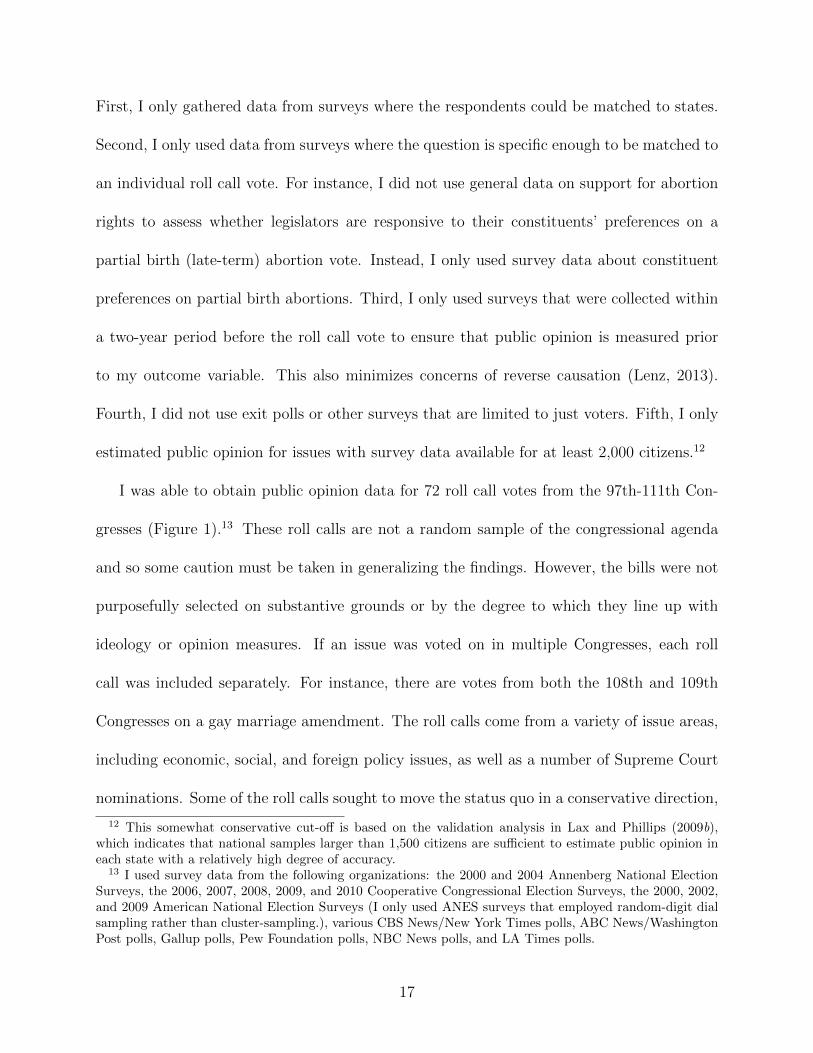
I was able to obtain public opinion data for 72 roll call votes from the 97th-111th Con-

gresses (Figure 1).13 These roll calls are not a random sample of the congressional agenda

and so some caution must be taken in generalizing the findings. However, the bills were not

purposefully selected on substantive grounds or by the degree to which they line up with

ideology or opinion measures. If an issue was voted on in multiple Congresses, each roll

call was included separately. For instance, there are votes from both the 108th and 109th

Congresses on a gay marriage amendment. The roll calls come from a variety of issue areas,

including economic, social, and foreign policy issues, as well as a number of Supreme Court

nominations. Some of the roll calls sought to move the status quo in a conservative direction,

12 This somewhat conservative cut-o↵ is based on the validation analysis in Lax and Phillips (2009b),which indicates that national samples larger than 1,500 citizens are su�cient to estimate public opinion ineach state with a relatively high degree of accuracy.

13 I used survey data from the following organizations: the 2000 and 2004 Annenberg National ElectionSurveys, the 2006, 2007, 2008, 2009, and 2010 Cooperative Congressional Election Surveys, the 2000, 2002,and 2009 American National Election Surveys (I only used ANES surveys that employed random-digit dialsampling rather than cluster-sampling.), various CBS News/New York Times polls, ABC News/WashingtonPost polls, Gallup polls, Pew Foundation polls, NBC News polls, and LA Times polls.

17

while others sought to move it in a liberal direction.

●●●●●●●●●●●●

●●●●●●●●●●●●●●●●●●●●●●●●●●●●●●●●●●●●●●●●●●●●

●●●●●●●●●●

●●●●●

●

0.00 0.25 0.50 0.75 1.00

Handgun Regulations (1991)Expand Medicaid for Poor Kids (2007)

Minimum Wage (2006)Minimum Wage (1996)

Brady Bill (1993)Minimum Wage (1989)Minimum Wage (2007)

Elena Kagan confirmation (2010)Minimum Wage (2000)Citizens United (2010)Nuclear Freeze (1983)

Assault Weapons Ban (1993)Expand Medicaid for Poor Kids (2009)

Art and Obscenity (1989)Clean Air Amendments (1990)

Family Leave (1992)Iran Contra Aid (1986)

Campaign Finance Reform (2002)Sonia Sotomayor confirmation (2009)

Raise Medicare Age to 67 (1997)Const. Amend. to Ban Abortion (1983)Const. Amend. to Ban Abortion (1982)

Financial reform (2010)Recovery (2009)

Surgeon General Confirmation (1995)Tax Increase on Tobacco (1998)

Immigration Reform (2006)Extend Unemployment Benefits (1992)

Immigration Reform (2007)Withdraw from Iraq (2007)

Defund Planned Parenthood (2011)Stem Cell Funding (2006)

Iran Contra Aid (1988)Drilling in ANWR (2002)

NAFTA (1993)Withdraw from Iraq (2006)Withdraw from Iraq (2005)Late−term Abortion (1999)

School Vouchers (2001)CAFTA (2005)

Bush Tax Cuts (2003)Gay Marriage Amendment (2006)

FISA (2008)Bork Nomination (1987)

Healthcare Reform (2009)Ban Discrimination Against Gays (1996)

Gays in the Military (1993)Cuba Sanctions (1999)

Tax Increase (1990)Capital Gains Tax Cut (1989)

Flag Burning Amendment (2006)Kuwaiti Tankers (1987)

Gay Marriage Amendment (2004)Late−term Abortion (1997)Iraq War Resolution (2002)

Capital Gains Tax (2006)Bush Tax Cuts (2001)

Patriot Renewal (2006)Estate Tax (2002)

Fed. Money for Abortions (2009)Samuel Alito confirmation (2006)

Estate Tax (2006)Clarence Thomas confirmation (1991)

John Roberts confirmation (2005)Balanced Budget Amend. (1997)

Federal Death Penalty (1984)Tax Cuts (1981)

Balanced Budget Amend. (1982)Parental Notific. of Abortion (2006)School Prayer Amendment (1984)

Parental Notific. of Abortion (1990)Welfare Reform (1996)

Public Opinion (1=Conservative Choice)

Figure 1: Public Opinion on each issue - This figure shows MRP estimates of public opinion.The dots show opinion in the median state, the thick lines show opinion in the middle 50percent of states, and the thin lines shows opinion over the entire range. To illustrate howopinion varies within states across issues, the triangles show opinion in New York and thesquares show opinion in Texas.

18

Figure 1 shows public opinion for each of the roll calls in my dataset. It indicates that

opinion varies significantly across issues. On some issues, there are clear liberal majorities,

while there are strong conservative majorities on other issues. The most liberal opinion

majorities are on handgun registration and expanding Medicaid for poor children. On the

other end of the spectrum, the most conservative opinion majorities are for welfare reform,

parental notification of abortion, and school prayer.

Issue-Specific Results

I run two sets of multi-level logistic regression models to examine the impact of election

proximity on Senators’ roll call votes. First, I analyze the association between public opinion

and roll call votes (“responsiveness”) through a set of models that examine whether variation

in public opinion is correlated with roll call votes after controlling for other factors (Achen,

1978; Egan, 2005). In these models, I interact the proximity of the next election with public

opinion to see how the association between public opinion and roll call votes varies over the

electoral cycle. I also include legislators’ party ID, as well as issue and legislator random/fixed

e↵ects.

It could be the case that members of Congress are responsive to public opinion, but

systemically more liberal, or conservative, than their constituencies (Achen, 1978; Erikson

and Wright, 2000). Thus, the concept of congruence assesses whether legislators follow the

preferences of a majority of their constituents on individual roll call votes (Egan, 2005;

Krimmel, Lax, and Phillips, 2015; Weissberg, 1979). I analyze congruence through a set of

models that examine whether election proximity a↵ects the probably that legislators’ votes

19

are congruent with the views of the majority of citizens in their state.

Dependent variable:

Rollcall Vote

(1) (2) (3) (4) (5)

Issue-Specific Public Opinion 5.01⇤⇤⇤ 4.69⇤⇤⇤ 4.80⇤⇤⇤ 4.84⇤⇤⇤ 2.96⇤⇤⇤

(0.0004) (0.62) (0.62) (0.62) (0.90)

Public Opinion * Last two years 1.85⇤⇤⇤ 1.78⇤⇤⇤ 1.45⇤⇤⇤ 1.39⇤⇤⇤ 1.68⇤⇤⇤

(0.0004) (0.45) (0.47) (0.47) (0.51)

Last two years �0.76⇤⇤⇤ �0.73⇤⇤⇤ �0.79⇤⇤⇤ �0.79⇤⇤⇤ �0.86⇤⇤⇤

(0.0004) (0.23) (0.23) (0.23) (0.25)

Last two years:Democrat 0.42⇤⇤ 0.44⇤⇤ 0.39⇤

(0.20) (0.19) (0.21)

Democrat �5.15⇤⇤⇤ �5.30⇤⇤⇤ �5.29⇤⇤⇤

(0.38) (0.39) (0.38)

Democratic Presidential Share �7.06⇤⇤⇤ �7.02⇤⇤⇤ �7.23⇤⇤⇤

(1.14) (1.14) (1.13)

Constant �2.84⇤⇤⇤ 3.85⇤⇤⇤ 3.85⇤⇤⇤ 3.89⇤⇤⇤ 0.18(0.0004) (0.67) (0.67) (0.66) (1.42)

Random E↵ects for Party x Issue X X X XRandom E↵ects for Legislator X X X XFixed E↵ects for Party x Issue XFixed E↵ects for Legislator X

Observations 7,094 7,094 7,094 7,275 7,094Log Likelihood �2,285.02 �2,208.13 �2,205.86 �2,252.60 �1,617.77Akaike Inf. Crit. 4,586.04 4,436.27 4,433.73 4,527.21 4,083.54Bayesian Inf. Crit. 4,640.97 4,504.94 4,509.26 4,603.02

Note: ⇤p<0.1; ⇤⇤p<0.05; ⇤⇤⇤p<0.01

Table 2: Senators’ Responsiveness to Public Opinion

Is there a stronger association between issue-specific public opinion and roll call votes

when elections are proximate? Using a model with random e↵ects for legislators and bills,

20

0.00 0.25 0.50 0.75 1.00

0.00

0.25

0.50

0.75

1.00

Public Opinion (1=Conservative)

Incr

ease

in P

rob.

of C

onse

rv. V

ote

Effect of Election Year on Responsiveness

0.00 0.25 0.50 0.75 1.00

0.00

0.25

0.50

0.75

1.00

Public Opinion (1=Conservative)

Incr

ease

in P

rob.

of C

onse

rv. V

ote

Among Republicans

0.00 0.25 0.50 0.75 1.00

0.00

0.25

0.50

0.75

1.00

Public Opinion (1=Conservative)

Incr

ease

in P

rob.

of C

onse

rv. V

ote

Among Democrats

Figure 2: Issue-Specific Responsiveness - This figure shows the association between variationin issue-specific public opinion and Senators’ roll call votes. The dotted lines show theassociation between opinion and votes during the last two years of senators’ terms and thedashed lines show the association during the remainder of the term.

Columns 1-4 of Table 2 show that, on average, Senators are more responsive to public opinion

in the last two years of their term. Indeed, Senators are about 25 percent more responsive

when elections are proximate. These results are robust across modeling specifications. In

addition, Column 5 shows that a model with fixed e↵ects for legislators and bills yields

similar results. Figure 2 plots the substantive meaning of these results. When 75 percent of

the public supports a liberal policy, there is a 38 percent probability that Republicans in the

last two years of their term will support the liberal policy, compared with just a 30 percent

probability of supporting the liberal policy for Republicans that are not in the last two years

21

of their term. Likewise, when 75 percent of the public supports a conservative policy, there is

a 51 percent probability that Democrats in the last two years of their term will support the

conservative policy, compared with a 35 percent probability of supporting the conservative

policy for Democrats that are not in the last two years of their term.

Table 3:

Dependent variable:

Congruent

(1) (2)

Size of Issue-Specific Majority 5.90⇤⇤⇤ 7.29⇤⇤⇤

(0.58) (0.71)

Last two years 0.13⇤⇤ 0.10(0.07) (0.07)

Democrat 0.73(0.46)

Constant �3.46⇤⇤⇤ �17.50(0.47) (6,522.65)

Random E↵ects for Party x Issue XRandom E↵ects for Legislator XFixed E↵ects for Party x Issue XFixed E↵ects for Legislator X

Observations 7,094 7,094Log Likelihood �3,267.38 �2,802.42Akaike Inf. Crit. 6,550.76 6,448.85Bayesian Inf. Crit. 6,605.70

Note: ⇤p<0.1; ⇤⇤p<0.05; ⇤⇤⇤p<0.01

Table 4: Congruence with Public Opinion, by Party

Moving beyond responsiveness, are Senators’ votes congruent with the preferences of a

majority of their constituents (Table 4)?14 Columns 1 and 2 show the average e↵ect of election

14 On the whole, about 60 percent of the roll call votes in my dataset are congruent with the views of

22

proximity on congruence across all Senators. Column 1 uses random e↵ects and column 2

uses fixed e↵ects. Both models indicate that Senators are somewhat more congruent with

issue-specific public opinion in the last two years of their term. This is broadly consistent with

evidence from a variety of previous studies that Senators tend to moderate their behavior in

the last two years of their term, since more moderate positions are generally more proximate

to the location of the median voter.

Conclusion

The foundation of representative democracy is the assumption that citizens’ preferences

should correspond with, and inform, elected o�cials’ behavior. Thus, in order to understand

how well our democracy is functioning, it is crucial to know the degree to which legislators

actually follow the views of their constituents. In this study, I show that there is a significant

relationship between public opinion and Senators’ roll call votes, both at an aggregate level

and on individual issues. But my results also indicate that the aggregate e↵ect of public

opinion is still small.

In addition, I resolve earlier ambiguities in the literature about the relationship between

election proximity and responsiveness over the past six decades. Three decades after Fenno’s

pathbreaking study of representation in the Senate, the literature on the relationship between

election proximity and responsiveness has remained ambiguous. This study demonstrates

issue-specific opinion majorities. The level of congruence between legislators’ roll calls and the majority ofthe public varies significantly across issues though. To put the level of congruence I find in context, it canbe compared to studies of specific issue areas in Congress. Krimmel, Lax, and Phillips (2015) find that 64percent of recent Congressional roll calls on gay rights are congruent with majority opinion. Kastellec, Lax,and Phillips (2010) find that Senators’ Supreme Court votes are congruent with public opinion 79 percentof the time.

23

that over the past six decades responsiveness in the United States Senate has predictably

varied over the course of the electoral cycle. My results provide strong support for the notion

that Senators are more attentive to their constituents’ views later in the electoral cycle. The

results here complement earlier findings that Senators move toward the electoral middle

when elections approach (Albouy, 2011; Amacher and Boyes, 1978; Elling, 1982; Lindstadt

and Vander Wielen, 2011; Thomas, 1985), as well as more recent findings that appropriations

are influenced by the electoral cycle (Shepsle et al., 2009).

Future work should examine other areas such as legislative e↵ort and constituent service

to examine whether they also vary over the electoral cycle. It should also examine other

legislative contexts such as state legislatures, where many states vary term lengths across

upper house districts (Titiunik, Forthcoming).15

15 Of course, it is possible that the lower salience of elections at the state-level reduces the incentives forlegislators there to respond to changes in public opinion.

24

References

Achen, Christopher H. 1978. “Measuring Representation.” American Journal of Political

Science 22(3): 475–510.

Achen, Christopher H, and Larry M Bartels. 2004. Musical chairs: Pocketbook voting and the

limits of democratic accountability. In Annual Meeting of the American Political Science

Association, Chicago.

Ahuja, Sunil. 1994. “Electoral Status and Representation in the United States Senate Does

Temporal Proximity to Election Matter?” American Politics Research 22(1): 104–118.

Albouy, David. 2011. “Do voters a↵ect or elect policies? A new perspective, with evidence

from the US Senate.” Electoral Studies 30(1): 162–173.

Amacher, Ryan C, and William J Boyes. 1978. “Cycles in Senatorial Voting Behavior:

Implications for the Optimal Frequency of Elections.” Public Choice 33(3): 5–13.

Angrist, Joshua David, and Jorn-Ste↵en Pischke. 2009. Mostly Harmless Econometrics: An

Empiricist’s Companion. Princeton, NJ: Princeton University Press.

Ansolabehere, Stephen, and Philip Edward Jones. 2010. “Constituents’ Responses to Con-

gressional Roll-Call Voting.”American Journal of Political Science 54(3): 583–597.

Ansolabehere, Stephen, James M. Snyder, Jr., and Charles Stewart, III. 2001. “Candidate

Positioning in U.S. House Elections.” American Journal of Political Science 45(1): 136–

159.

Arnold, R Douglas. 1992. The Logic of Congressional Action. Yale University Press.

25

Beck, Nathaniel, and Jonathan N Katz. 2011. “Modeling Dynamics in Time-Series-Cross-

section Political Economy Data.”Annual Review of Political Science 14: 331–352.

Broockman, David E. 2016. “Approaches to Studying Policy Representation.” Legislative

Studies Quarterly .

Buttice, Matthew K, and Benjamin Highton. Forthcoming. “Assessing the Mechanisms of

Senatorial Responsiveness to Constituency Preferences.”American Politics Research .

Canes-Wrone, Brandice, David W. Brady, and John F. Cogan. 2002. “Out of Step, Out of

O�ce: Electoral Accountability and House Members’ Voting.”American Political Science

Review 96(1): 127–140.

Caughey, Devin, and Christopher Warshaw. 2015. “Dynamic Estimation of Latent Opinion

Using a Hierarchical Group-Level IRT Model.” Political Analysis 23(2): 197–211.

Caughey, Devin, and Christopher Warshaw. 2016. “Dynamic Representation in the American

States, 1936-2014.” Paper presented at the 2016 State Politics Conference.

Caughey, Devin, and Eric Schickler. 2014. “Structure and Change in Congressional Ideology:

NOMINATE and Its Alternatives.” Paper presented at the 2014 Congress and History

Conference, University of Maryland, College Park, June 11, 2014.

Clinton, Joshua D. 2006. “Representation in Congress: Constituents and Roll Calls in the

106th House.” Journal of Politics 68(2): 397–409.

Clinton, Joshua, Simon Jackman, and Douglas Rivers. 2004. “The Statistical Analysis of

Roll Call Data.”American Political Science Review 98(2): 355–370.

26

De Boef, Suzanna, and Luke Keele. 2008. “Taking Time Seriously.” American Journal of

Political Science 52(1): 184–200.

Downs, Anthony. 1957. An Economic Theory of Democracy. New York, NY: Harper and

Row.

Egan, Patrick J. 2005. “Policy Preferences and Congressional Representation: The Relation-

ship Between Public Opinion and Policymaking in Today’s Congress.”.

Elling, Richard C. 1982. “Ideological Change in the US Senate: Time and Electoral Respon-

siveness.” Legislative Studies Quarterly 7(1): 75–92.

Ellis, Christopher, and James A. Stimson. 2012. Ideology in America. New York: Cambridge

UP.

Ensley, Michael J. 2007. “Candidate divergence, ideology, and vote choice in US Senate

elections.”American Politics Research 35(1): 103–122.

Erikson, Robert S, and Gerald C Wright. 2000. “Representation of Constituency Ideology

in Congress.” In Continuity and Change in House Elections, ed. David W Brady, John F

Cogan, and Morris P Fiorina. Stanford: Stanford University Press pp. 149–77.

Erikson, Robert S., Gerald C. Wright, and John P. McIver. 1993. Statehouse Democracy:

Public Opinion and Policy in the American States. New York: Cambridge University

Press.

Erikson, Robert S., Gerald C. Wright, and John P. McIver. 2006. “Public Opinion in the

27

States: A Quarter Century of Change and Stability.” In Public Opinion in State Politics,

ed. Je↵rey E. Cohen. Palo Alto, CA: Stanford University Press pp. 229–253.

Erikson, Robert S., Gerald C. Wright, and John P. McIver. 2007. “Measuring the Public’s

Ideological Preferences in the 50 states: Survey Responses versus Roll Call Data.” State

Politics & Policy Quarterly 7(2): 141–151.

Fenno, Richard F. 1982. The United States Senate: A Bicameral Perspective. American

Enterprise Institute for Public Policy Research Washington, DC.

Franklin, Charles H. 1993. “Senate incumbent visibility over the election cycle.” Legislative

Studies Quarterly pp. 271–290.

Gilens, Martin. 2005. “Inequality and Democratic Responsiveness.” The Public Opinion

Quarterly 69(5): 778–796.

Hall, Andrew. 2015. “What Happens When Extremists Win Primaries?” The American

Political Science Review 109(1): 18.

Healy, Andrew, and Gabriel S Lenz. 2014. “Substituting the End for the Whole: Why Voters

Respond Primarily to the Election-Year Economy.”American Journal of Political Science

58(1): 31–47.

Henderson, John, and John Brooks. Forthcoming. “Mediating the Electoral Connection: The

Information E↵ects of Voter Signals on Legislative Behavior.”The Journal of Politics .

Huber, Gregory A, Seth J Hill, and Gabriel S Lenz. 2012. “Sources of bias in retrospective

28

decision making: Experimental evidence on voters’ limitations in controlling incumbents.”

American Political Science Review 106(04): 720–741.

Huber, Gregory, and Sanford C Gordon. 2004. “Accountability and Coercion: Is Justice

Blind When it Runs for O�ce?” American Journal of Political Science 48(2): 247–263.

Jessee, Stephen. 2016. “(How) Can We Estimate the Ideology of Citizens and Political Elites

on the Same Scale?” American Journal of Political Science .

Jessee, Stephen A. 2009. “Spatial voting in the 2004 presidential election.”American Political

Science Review 103(1): 59–81.

Kastellec, Jonathan P, Je↵rey R Lax, and Justin H Phillips. 2010. “Public Opinion and

Senate Confirmation of Supreme Court Nominees.” Journal of Politics 72(3): 767–784.

Kousser, Thad, Je↵rey B Lewis, and Seth E Masket. 2007. “Ideological Adaptation? The

Survival Instinct of Threatened Legislators.” Journal of Politics 69(3): 828–843.

Krimmel, Katherine L, Je↵rey R Lax, and Justin H Phillips. 2015. “Gay Rights in Congress:

Public Opinion and (Mis)Representation.” Public Opinion Quarterly forthcoming.

Lax, Je↵rey R., and Justin H. Phillips. 2009a. “Gay Rights in the States: Public Opinion

and Policy Responsiveness.”American Political Science Review 103(3): 367–386.

Lax, Je↵rey R., and Justin H. Phillips. 2009b. “How Should We Estimate Public Opinion in

The States?” American Journal of Political Science 53(1): 107–121.

Lax, Je↵rey R., and Justin H. Phillips. 2011. “The Democratic Deficit in the States.”Amer-

ican Journal of Political Science 56(1): 148–166.

29

Lee, David S., Enrico Moretti, and Matthew J. Butler. 2004. “Do Voters A↵ect Or Elect

Policies? Evidence From the U. S. House.”Quarterly Journal of Economics 119(3): 807–

859.

Lenz, Gabriel S. 2013. Follow the Leader?: How Voters Respond to Politicians’ Policies and

Performance. University of Chicago Press.

Levendusky, Matthew S., Jeremy C. Pope, and Simon D. Jackman. 2008. “Measuring

District-Level Partisanship with Implications for the Analysis of US Elections.” Journal of

Politics 70(3): 736–753.

Levitt, Steven D. 1996. “How Do Senators Vote? Disentangling the Role of Voter Preferences,

Party A�liation, and Senator Ideology.”American Economic Review 86(3): 425–441.

Lewis, Je↵rey B., and Chris Tausanovitch. 2013. “Has Joint Scaling Solved the Achen Objec-

tion to Miller and Stokes.” Paper presented at Political Representation: Fifty Years after

Miller & Stokes, Center for the Study of Democratic Institutions, Vanderbilt University,

Nashville, TN, March 1–2, 2013.

Lindstadt, Rene, and Ryan J Vander Wielen. 2011. “Timely Shirking: Time-Dependent

Monitoring and its E↵ects on Legislative Behavior in the US Senate.”Public Choice 148(1):

119–148.

Martin, Andrew D., and Kevin M. Quinn. 2002. “Dynamic Ideal Point Estimation via

Markov Chain Monte Carlo for the U.S. Supreme Court, 1953–1999.” Political Analysis

10(2): 134–153.

30

Matsusaka, John G. 2010. “Popular Control of Public Policy: A Quantitative Approach.”

Quarterly Journal of Political Science 5(2): 133–167.

Mayhew, David. 1974. The Electoral Connection. New Haven: Yale University Press.

Miler, Kristina. Forthcoming. “Legislative Responsiveness to Constituency Change.”Amer-

ican Politics Research .

Miller, Warren E., and Donald E. Stokes. 1963. “Constituency Influence in Congress.”Amer-

ican Political Science Review 57(1): 45–56.

Nokken, Timothy P., and Keith T. Poole. 2004. “Congressional Party Defection in American

History.” Legislative Studies Quarterly 29(4): 545–568.

Park, David K., Andrew Gelman, and Joseph Bafumi. 2004. “Bayesian Multilevel Estima-

tion with Poststratification: State-Level Estimates from National Polls.”Political Analysis

12(4): 375–385.

Park, David K., Andrew Gelman, and Joseph Bafumi. 2006. “State Level Opinions from Na-

tional Surveys: Poststratification Using Multilevel Logistic Regression.” In Public Opinion

in State Politics, ed. Je↵rey E. Cohen. Stanford, CA: Stanford University Press pp. 209–

228.

Poole, Keith T. 2007. “Changing Minds? Not in Congress!” Public Choice 131(3-4): 435–451.

Poole, Keith T, and Howard Rosenthal. 2000. Congress: A political-economic history of roll

call voting. Oxford University Press, USA.

31

Ruggles, Steven, J. Trent Alexander, Katie Genadek, Ronald Goeken, Matthew B. Schroeder,

and Matthew Sobek. 2010. “Integrated Public Use Microdata Series: Version 5.0 [Machine-

readable database].” Minneapolis: University of Minnesota.

Shapiro, Catherine R, David W Brady, Richard A Brody, and John A Ferejohn. 1990. “Link-

ing Constituency Opinion and Senate Voting Scores: A Hybrid Explanation.” Legislative

Studies Quarterly pp. 599–621.

Shepsle, Kenneth A, Robert P Van Houweling, Samuel J Abrams, and Peter C Hanson. 2009.

“The Senate Electoral Cycle and Bicameral Appropriations Politics.”American Journal of

Political Science 53(2): 343–359.

Shor, Boris, and Jon C Rogowski. 2013. Proximity Voting in Congressional Elections. In

Annual Meeting of the Mid-West Political Science Association, Chicago, IL.

Stimson, James A., Michael B. MacKuen, and Robert S. Erikson. 1995. “Dynamic Repre-

sentation.”American Political Science Review 89(3): 543–565.

Stratmann, Thomas. 2000. “Congressional voting over legislative careers: Shifting positions

and changing constraints.”American Political Science Review 94(03): 665–676.

Thomas, Martin. 1985. “Election Proximity and Senatorial Roll Call Voting.” American

Journal of Political Science 29(1): 96–111.

Titiunik, Rocio. Forthcoming. “Drawing Your Senator From a Jar: Term Length and Leg-

islative Behavior.” Political Science Research and Methods .

Van Houweling, Robert P, and Michael Tomz. 2011. Candidate Repositioning: How Voters

32

Respond When Incumbent Politicians Change Positions on Issues. In APSA 2011 Annual

Meeting Paper.

Weissberg, Robert. 1979. “Assessing Legislator-Constituency Policy Agreement.” Legislative

Studies Quarterly 4(04): 605–622.

Wood, B Dan, and Angela Hinton Andersson. 1998. “The dynamics of senatorial represen-

tation, 1952-1991.” Journal of Politics 60: 705–736.

Wright, Gerald C, and Michael B Berkman. 1986. “Candidates and Policy in United States

Senate Elections.”American Political Science Review 80(2): 567–588.

33

Appendix A: Methodology for Estimating Citizen Policy

Conservatism

The lack of a time-varying measure of citizens’ policy preferences in each state has been one

of the main barriers to the study of representation in Congress. To overcome this challenge, I

apply the dynamic hierarchical group-level IRT model developed by Caughey and Warshaw

(2015, 2016), which estimates the average policy conservatism of defined subpopulations (e.g.,

non-urban whites, urban whites, and blacks in each state). This model adopts the general

framework of item-response theory (IRT). In an IRT model, respondents’ question responses

are jointly determined by their score on some unobserved trait—such as their economic

policy conservatism—and by the characteristics of the particular question. The relationship

between responses to question q and the unobserved trait ✓

i

is governed by the question’s

threshold

qt

, which captures the base level of support for the question, and its dispersion

�

q

, which represents question-specific measurement error. Under this model, respondent i’s

probability of selecting the conservative response to question q is

⇡

iq

= �

✓✓

i

�

qt

�

q

◆, (1)

where the normal CDF � maps (✓i

�

qt

)/�q

to the (0, 1) interval.1 The model assumes that

greater conservatism (i.e., higher values of ✓i

) increases respondents’ probability of answering

in a conservative direction. The strength of this relationship is inversely proportional to �

q

,

and the threshold for a conservative response is governed by

qt

. The probability that a

1A common alternative way of writing the model in Equation (1) is Pr(yiq = 1) = �(�q✓i � ↵q), where

�q = 1/�q and ↵q = qt ⇥ �q.

1

randomly sampled member of group g correctly answers item q is

⇡

gq

= �

0

@ ✓

g

�

qtq�

2q

+ �

2✓

1

A, (2)

where �

✓

is the standard deviation of ✓i

within groups. Equation (2) is connected to the

data through the sampling model

s

gq

⇠ Binomial(ngq

, ⇡

gq

), (3)

where n

gq

is group g’s total number of non-missing responses to question q and s

gq

is the

number of those responses that are conservative.2 The estimates of ✓g

can be poststratified

into estimates of the average economic conservatism in each state (cf. Park, Gelman, and

Bafumi (2004)).

To address sparseness in the matrix of survey data, I use a dynamic linear model to

smooth the estimated group means across both time and states.

✓

gt

⇠ N(�t

✓

g,t�1 + ⇠

t

+ x0g·�t, �

2✓t

), (4)

where ✓

g,t�1 is g’s mean in the previous year, ⇠t

is a year-specific intercept, and xg· is a

vector of attributes of g (e.g., its state or party). Each group-year mean is thus modeled

as a function of the group’s mean in the previous year, year-specific changes common to all

groups, and changes in relative conservatism of groups with similar characteristics (i.e., the

2Following Ghitza and Gelman (2013) and Caughey and Warshaw (2015, 202–3), I adjust the raw values

of sgq and ngq to account for survey weights and for respondents who answer multiple questions.

2

same party or state). The posterior estimates of ✓gt

are a thus compromise between this

prior and the likelihood implied by Equations (2) and (3), with the relative weight placed on

the likelihood determined by the prior standard deviation �

✓t

, which is estimated from the

data and allowed to evolve across years. When a lot of survey data are available for a given

year, the likelihood will dominate. If no survey data are available at all, the prior acts as a

predictive model that imputes ✓gt

.

The dynamic group-level IRT model estimates opinion in groups defined by states and

demographic groups. To generate annual estimates of average opinion in each state, the

survey data are pre-weighted to match raked targets for gender and education level in each

state public, based on data from the U.S. Census (Ruggles et al., 2010). This model produces

estimates of the ideology of non-urban whites, urban whites, and blacks in each state. Finally,

the estimates are aggregated up to the national level based on post-stratification weights from

the PUMS data available from the Census.

3

Appendix B: MRP Methodology for Estimating Issue-

Specific Public Opinion

Multilevel regression and poststratification (MRP) models employ Bayesian statistics and

multilevel modeling to incorporate information about respondents’ demographics and ge-

ography in order to estimate public opinion in each geographic subunit (Park, Gelman,

and Bafumi, 2004; Lax and Phillips, 2009; Warshaw and Rodden, 2012). Specifically, each

individual’s survey responses are modeled as a function of demographic and geographic pre-

dictors, partially pooling respondents across state to an extent determined by the data (see

Gelman and Hill, 2007; Jackman, 2009 for more about multilevel modeling). The state-

level e↵ects are modeled using additional state-, and region-level predictors, such as states’

median-income level and religiosity. Thus, all individuals in the survey yield information

about demographic and geographic patterns, which can be applied to all state estimates.

The final step is poststratification, in which the estimates for each demographic-geographic

respondent type are weighted (poststratified) by the percentage of each type in the actual

state population.

There are two stages to the MRP model. In the first stage, I estimate each individual’s

preferences as a function of his or her demographics and and state (for individual i, with

indexes r, e, a, p, s, and z for race, gender, education category, poll, state, and region,

respectively). This approach allows individual-level demographic factors and geography to

contribute to my understanding of state opinion. Moreover, the model incorporates both

within and between state geographic variation. I facilitate greater pooling across states by

including in the model several state-level variables that are plausibly correlated with public

4

opinion. For example, I include the percentage of people in each state that are evangelicals

or Mormons.

I incorporate this information with the following hierarchical model for respondent’s

responses:

Pr(yi

= 1) = logit

�1(�0 + ↵

race

r[i] + ↵

gender

g[i] + ↵

edu

e[i] + ↵

age

a[i] + ↵

state

s[i] + ↵

poll

p[i] )

where:

↵

race

r[i] for r = 1, 2

↵

gender

g[i] for g = 1, 2

↵

edu

e[i] for e = 1, . . . , 5

↵

poll

p[i] for p = the number of polls for each issue

(5)

That is, each individual-level variable is modeled as drawn from a normal distribution

with mean zero and some estimated variance. Following previous work using MRP, I assume

that the e↵ect of demographic factors does not vary geographically. I allow geography to

enter into the model by adding a state level to the model, and giving each state a separate

intercept.

The state e↵ects are modeled as a function of the region into which the state falls,

the percentage of the state’s residents that are union members, the state’s percentage of

evangelical or Mormon residents, the state’s average income, and the percent of the state’s

residents that live in urban areas.

↵

state

s

v N(↵region

z

+ �1 ⇤ unions

+ �2 ⇤ religions

+ �3 ⇤ income

s

+ �4 ⇤ urbans

, �

2s

)

for s = (1, . . . , 51)

(6)

The region variable is, in turn, another modeled e↵ect. I group states into regions based on

5

their general ideology and vote in presidential elections.

↵

region

z[i] v N(0, �2z

)

for z = (1, . . . , 6)

(7)

I estimate the model using the GLMER function in R (Bates 2005).

Poststratification

For any set of individual demographic and geographic values, cell c, the results above allow me

to make a prediction of public opinion. Specifically, c is a function of the relevant predictors

and their estimated coe�cients. Next, I weight these estimates by the percentages of each

type in the actual state populations. I calculate the necessary population frequencies using

PUMS “5-Percent Public Use Microdata Sample” from the census, which has demographic

information for 5 percent of each state’s voting- age population (Park, Gelman, and Bafumi,

2004; Lax and Phillips, 2009).

Validation

The MRP estimates of state-level public opinion are generally highly correlated with the raw

”disaggregated” state-level estimates of public opinion from the various surveys. Across all

issues, the MRP estimates of public opinion are correlated with the disaggregated estimates

at 0.91. For roll calls with smaller sample sizes, however, there are sometimes smaller

correlations between the disaggregated and MRP estimates. The advantage of MRP is that

it enables me to accurately estimate public opinion for issues, such as closing Guantanamo,

6

or geographic areas, such as Montana and North Dakota, where survey data is sparse.

7

References

Caughey, Devin, and Christopher Warshaw. 2015. “Dynamic Estimation of Latent Opinion

Using a Hierarchical Group-Level IRT Model.” Political Analysis 23(2): 197–211.

Caughey, Devin, and Christopher Warshaw. 2016. “Dynamic Representation in the American

States, 1936-2014.” Paper presented at the 2016 State Politics Conference.

Gelman, Andrew, and Jennifer Hill. 2007. Data analysis using regression and multi-

level/hierarchical models. Cambridge University Press.

Ghitza, Yair, and Andrew Gelman. 2013. “Deep Interactions with MRP: Election Turnout

and Voting Patterns Among Small Electoral Subgroups.” American Journal of Political

Science 57(3): 762–776.

Jackman, Simon. 2009. Bayesian Analysis for the Social Sciences. Hoboken, NJ: Wiley.

Lax, Je↵rey R., and Justin H. Phillips. 2009. “How Should We Estimate Public Opinion in

The States?” American Journal of Political Science 53(1): 107–121.

Park, David K., Andrew Gelman, and Joseph Bafumi. 2004. “Bayesian Multilevel Estima-

tion with Poststratification: State-Level Estimates from National Polls.”Political Analysis

12(4): 375–385.

Ruggles, Steven, J. Trent Alexander, Katie Genadek, Ronald Goeken, Matthew B. Schroeder,

and Matthew Sobek. 2010. “Integrated Public Use Microdata Series: Version 5.0 [Machine-

readable database].” Minneapolis: University of Minnesota.

8

Warshaw, Christopher, and Jonathan Rodden. 2012. “How Should We Measure District-Level

Public Opinion on Individual Issues?” Journal of Politics 74(1): 203–219.

9