response-adaptive randomization (rar) in …yw2148/abstracts/columbia-feifang.pdf1 response-adaptive...
TRANSCRIPT

1
Response-Adaptive Randomization (RAR) inClinical Trials
Feifang Hu
Department of Statistics
University of Virginia
and
Division of Biostatistics and Epidemiology
Department of Health Evaluation Science
University of Virginia School of Medicine
Email: [email protected]
Nov 15, 2007, at Columbia University
2
Outline
• Motivating examples.
• Overview of the problem.
• Brief review of adaptive randomization.
• Power and variability.
• Best randomization procedures.
• Doubly-adaptive biased coin designs.
• Some recent developments.
• Further topics.
• Future of RAR.
1 One Motivating Example. 3
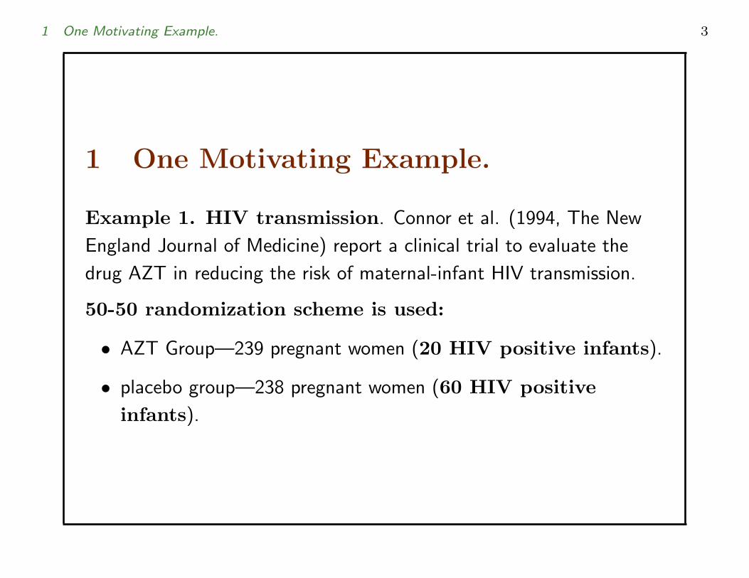
1 One Motivating Example.
Example 1. HIV transmission. Connor et al. (1994, The New
England Journal of Medicine) report a clinical trial to evaluate the
drug AZT in reducing the risk of maternal-infant HIV transmission.
50-50 randomization scheme is used:
• AZT Group—239 pregnant women (20 HIV positive infants).
• placebo group—238 pregnant women (60 HIV positiveinfants).

1 One Motivating Example. 4
Given the seriousness of the outcome of this study, it is reasonable to
argue that 50-50 allocation was unethical. As accruing information
favoring (albeit, not conclusively) the AZT treatment became
available, allocation probabilities should have been shifted from50-50 allocation proportional to weight of evidence forAZT. Designs which attempt to do this are called Response-Adaptive
designs (Response-Adaptive Randomization).

1 One Motivating Example. 5
If the treatment assignments had been done with the randomizedplay the winner rule (RPW rule) (Zelen 1969, JASA, Wei and
Durham,1978, JASA):
• AZT Group— 360 patients
• placebo group—117 patients
then, only 60 (instead of 80) infants would be HIV positive.

1 One Motivating Example. 6
Example 2 (ECMO Trial). Extracorporeal membrane oxygenation
(ECMO) is an external system for oxygenating the blood based on
techniques used in cardiopulmonary bypass technology developed for
cariac surgery. In the literature, there are three well-document clinical
trials on evaluating the clinical effectiveness of ECMO:
(i) the Michigan ECMO study (Bartlett, et al. 1985);
(ii) the Boston ECMO study (Ware, 1989);
(iii) the UK ECMO trial (UK Collaborative ECMO Trials Group, 1996).

1 One Motivating Example. 7
The UK ECMO trial:
50-50 randomization scheme is used:
• ECMO Group—93 infants (28 deaths).
• Conventional group—92 infants (54 deaths).
If ERADE (Hu, Zhang and He, 2007) is used, then
• ECMO Group—121 infants (36 deaths).
• Conventional group—64 infants (38 deaths).

2 Overview of the Problem. 8
2 Overview of the Problem.
Clinical Trials: Complex with multiple (competitive) objectives
• maximizing power to detect clinically relevant difference;
• minimizing the expected total number of failures;
• maximizing the individual patient’s experience in the trial;
• minimizing total monetary cost of trial;
• etc.
Randomized designs should be used to remove the potential bias in
clinical trial.

2 Overview of the Problem. 9
Example 3. Binary response: treatment A and B.
• pA: P (success|A), qA = 1− pA;
• pB : P (success|B), qB = 1− pB ;
• nA: number of patients on A;
• nB : number of patients on B, n = nA + nB .

2 Overview of the Problem. 10
Some important functions:
1 An objective function, φ(nA, nB), power or noncentral parameter;
2 Sample size nA + nB or total number of failures qAnA + qBnB ;
3 Allocation proportion to treatment A, ρ(pA, pB) ∼ nA/n;
Approach 1:
With fixed φ(nA, nB), to minimizing sample size, n = nA + nB , the
solution is called Neyman allocation:
ρ(pA, pB) =√
pAqA√pAqA +
√pBqB
.

2 Overview of the Problem. 11
Approach 2:
With fixed φ(nA, nB), to minimizing total number of failures,
qAnA + qBnB , the solution is called optimal allocation (see
Rosenberger et al. (2001, biometrics)):
ρ(pA, pB) =√
pA√pA +
√pB
.
Tymofyeyev, Rosenberger and Hu (2007, JASA) propose a general
framework to find optimal ρ.

2 Overview of the Problem. 12
Usually ρ(pA, pB) depends on unknown parameters, how to
implement these optimal allocations?
Solution: Response-Adaptive Randomization can beapplied to achieve above objectives.

2 Overview of the Problem. 13
Three-step approach:
1. Find the optimal allocation;
2. Use sequential estimation, substituting estimates from the data
accrued thus far into the optimal allocation;
3. Find an appropriate randomization procedure that will result in
optimal allocation.
We call the resulting randomization procedure a response-adaptive
randomization procedure, because the probability of assignment to
treatments will depend on previous patient responses.

3 Brief review of Adaptive Randomization 14
3 Brief review of Adaptive
Randomization
3.1 Adaptive Randomization for Balancing
Complete randomization: Assign next patient to A with
probability 0.5.
Disadvantages: unbalance among A and B (usually not powerful).

3 Brief review of Adaptive Randomization 15
Some important designs:
• Truncated binomial design.
• Permuted block designs.
• Efron’s biased coin design (Efron, 1971, Biometrika): Assign next
patient to A (or B) with probability 2/3, if there are more
patients in B (or A). Use complete randomization, if equal.
• Wei’s urn design (Wei, 1977, JASA and Wei, 1978, Annals).
• Generalized biased coin design (Smith, 1984, JRSSB).
3 Brief review of Adaptive Randomization 16
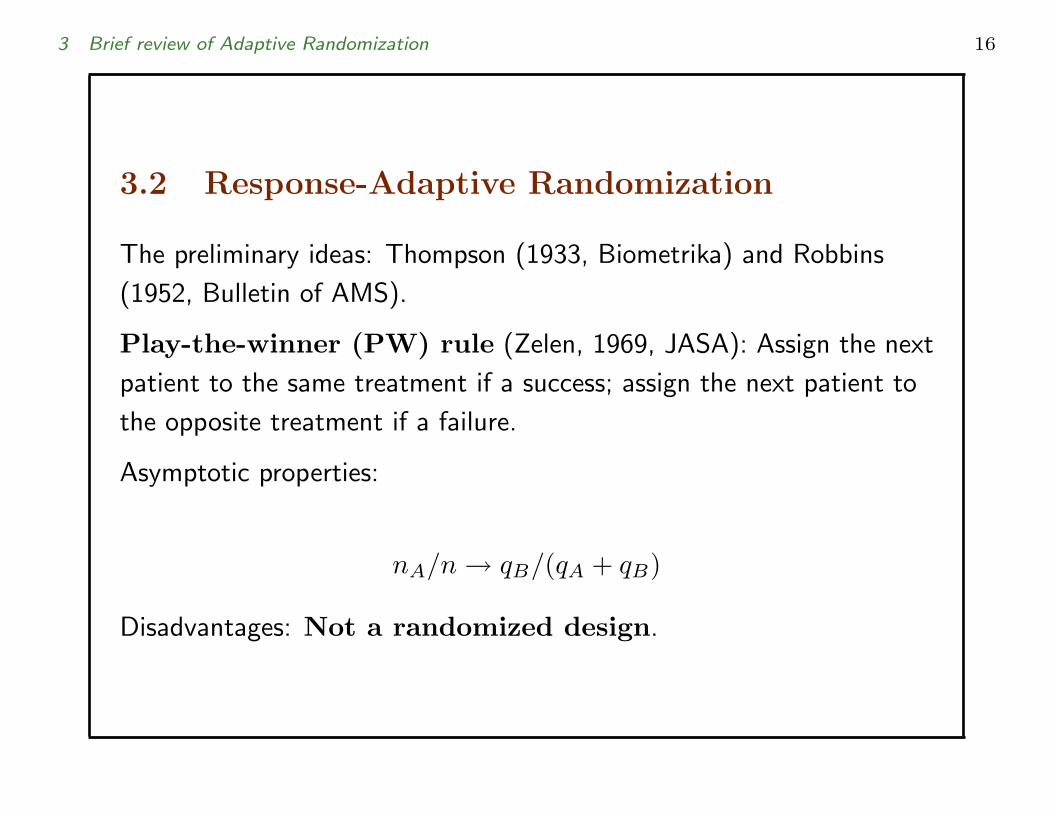
3.2 Response-Adaptive Randomization
The preliminary ideas: Thompson (1933, Biometrika) and Robbins
(1952, Bulletin of AMS).
Play-the-winner (PW) rule (Zelen, 1969, JASA): Assign the next
patient to the same treatment if a success; assign the next patient to
the opposite treatment if a failure.
Asymptotic properties:
nA/n → qB/(qA + qB)
Disadvantages: Not a randomized design.

3 Brief review of Adaptive Randomization 17
Randomized play-the-winner (RPW) rule (Wei and
Durham,1978, JASA).
Begin with c balls of A and c balls of B in an urn.
• Draw A:
– assign patient to A;
– replace ball;
– add 1 type A ball if treatment A is successful;
– add 1 type B ball if treatment A is failure.
• Draw B:
– assign patient to B;
– replace ball;
– add 1 type B ball if treatment B is successful;
– add 1 type A ball if treatment B is failure.

3 Brief review of Adaptive Randomization 18
Two main families:
(i) Urn models: PW rule; RPW rule; Generalized Friedman’s urn
models (Wei, 1979, JASA; Smythe, 1996, Stochastic Process. Appl.;
Bai, Hu and Shen, 2002, JMVA); Randomized Polya Urn (Durham,
Flournoy, and Li, 1998, CJS); Ternary Urn (Ivanova and Flournoy,
2001); Drop-the-Loser rule (Ivanova, 2003, Metrika); Generalized
drop-the-Loser rule (Zhang, Chan, Cheung and Hu, 2007, Statistic
Sinica), etc.
(ii) Doubly adaptive biased coin designs: Eisele and Woodroofe (1995,
Annals of Statistics), Hu and Zhang (2004, Annals of Statistics), Hu
and Rosenberger (2003, JASA). ERADE (Hu, Zhang and He, 2007).

3 Brief review of Adaptive Randomization 19
Example: Extracorporeal Membrane Oxygenation(ECMO) trial using RPW rule:The RPW rule was used in a clinical trial of extracorporeal membrane
oxygenation (ECMO; Bartlett, et al. 1985, Pediatrics), a surgical
procedure for newborns with respiratory failure.
Total 12 patients.
• ECMO group– 11 patients, all survived.
• Conventional therapy– 1 patient, died.
Valid of this trial??? No statistical conclusion.
Why??? Power and variability.
Another ECMO trial at England, 185 patients (93 inECMO and 92 in control), 82 patients died.
3 Brief review of Adaptive Randomization 20
In literature, researchers focused on:
(i) proposing new response-adaptive designs;
(ii) studying some properties;
(iii) comparing designs by simulations.
Some important questions:
• What is relationship among the power, expected failures and the
design?
• How to compare different designs?
• What is a good design?
• etc.
4 Power and Variability 21
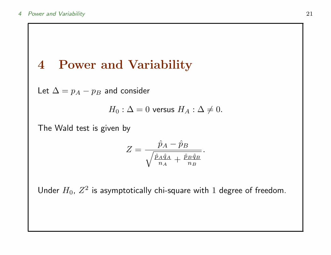
4 Power and Variability
Let ∆ = pA − pB and consider
H0 : ∆ = 0 versus HA : ∆ 6= 0.
The Wald test is given by
Z =p̂A − p̂B√
p̂Aq̂A
nA+ p̂B q̂B
nB
.
Under H0, Z2 is asymptotically chi-square with 1 degree of freedom.

4 Power and Variability 22
Under the HA, power is an increasing function of the the noncentrality
parameter:
φ =(pA − pB)2
pAqA/nA + pBqB/nB
=n(pA − pB)2
pAqA
ρ+(nA/n−ρ) + pBqB
(1−ρ)−(nA/n−ρ)
.
Now we define a function
f(x) =(pA − pB)2
pAqA/[ρ + x] + pBqB/[(1− ρ)− x].
We have the following expansion:
f(x) = f(0) + f ′(0)x + f ′′(0)x2/2 + o(x2).
After some calculation, we obtain
f ′(0) = (pA − pB)2(pAqA(1− ρ)2 − pBqBρ2)(pAqA(1− ρ) + pBqBρ)2

4 Power and Variability 23
and
f ′′(0) = −2(pA − pB)2pAqApBqB
((1− ρ)ρ)3.
The non-centrality parameter is
n−1φ =(pA − pB)2
pAqA/ρ + pBqB/(1− ρ)
+(pA − pB)2(pAqA(1− ρ)2 − pBqBρ2)(pAqA(1− ρ) + pBqBρ)2
(nA/n− ρ)
−(pA − pB)2pAqApBqB
((1− ρ)ρ)3(nA/n− ρ)2
+o((nA/n− ρ)2)
= (I) + (II) + (III) + o((nA/n− ρ)2)

4 Power and Variability 24
The first term (I) is determined by ρ, and represents the non-centrality
parameter for a fixed design (with ρ as the target allocation
proportion). Note that Neyman allocation maximizes this term.
The second term (II) represents the bias of the actual allocation from
the optimal allocation. With the design shifting to different side from
the target proportion ρ, the non-centrality parameter will increase or
decrease according the coefficient
(pA − pB)2(pAqA(1− ρ)2 − pBqBρ2)(pAqA(1− ρ) + pBqBρ)2
.
It is interesting to see that this coefficient equals 0 if and only if
pAqA(1− ρ)2 − pBqBρ2 = 0, that is
ρ =√
pAqA√pAqA +
√pBqB
,
i.e., Neyman allocation.

4 Power and Variability 25
Most procedures will be asymptotically unbiased, so we can assume
E(nA/n− ρ) = 0
for large n. Assuming this, the average power lost of the procedure is
then a function of
−(pA − pB)2pAqApBqB
((1− ρ)ρ)3E(nA/n− ρ)2,
which is a direct function of the variability of the design.
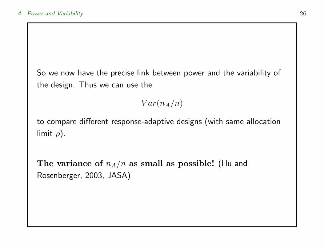
4 Power and Variability 26
So we now have the precise link between power and the variability of
the design. Thus we can use the
V ar(nA/n)
to compare different response-adaptive designs (with same allocation
limit ρ).
The variance of nA/n as small as possible! (Hu and
Rosenberger, 2003, JASA)

5 Best Adaptive Randomization Procedures 27
5 Best Adaptive Randomization
Procedures
Lower Bound of V ar(nA/n)?
Let I(pA, pB , nA) be the Fisher’s information, where the expectation
is taken conditional on nA, for estimating pA and pB . Suppose the
following some regularity conditions hold. Then the lower bound of
V ar(nA/n) is given by(∂ρ(pA, pB)
∂pA
∂ρ(pA, pB)∂pB
)I−1(pA, pB , ρ(n, pA, pB))
(∂ρ(pA, pB)
∂pA
∂ρ(pA, pB)∂pB
)′
.

5 Best Adaptive Randomization Procedures 28
We refer to a response-adaptive design that attains the lower bound as
asymptotically best for that particular target allocation ρ(pA, pB).
If
ρ(pA, pB) = qB/(qA + qB),
then the lower bound is
qAqB(pA + pB)(qA + qB)3
.
For general cases, see Hu and Rosenberger (2003, JASA) and Hu,
Rosenberger and Zhang (2006, JSPI) for details.

5 Best Adaptive Randomization Procedures 29
Asymptotic properties (pA + pB < 1.5) of RPW rule:
nA/n → qB/(qA + qB)
and√
n(nA/n− qB/(qA + qB)) →D N(0, σ2).
Where
σ2 =qAqB [5− 2(qA + qB)]
[2(qA + qB)− 1](qA + qB)2.
Not attain the lower bound

5 Best Adaptive Randomization Procedures 30
RPW rule (urn models)
• targets the urn allocation qB/(qA + qB);
• applies to binary responses only.
• does not attain the lower bound.
Can we find a design that
• can target any given allocation ρ;
• attain the low bound;
• and apply to other types of responses?
Yes.

6 Doubly-Adaptive Biased Coin Design 31
6 Doubly-Adaptive Biased Coin Design
Doubly-adaptive biased coin design (DBCD) (Eisele and Woodroofe,
1995, Annals of Statist, Hu and Zhang, 2004, Annals of Statist).
Let g be a function from [0, 1]× [0, 1] to [0, 1] satisfied certainly
conditions. The procedure then allocates patient j to treatment A
with probability
g(nA(j − 1)
j − 1, ρ̂).
How to choose function g?
Eisele and Woodroofe (1995) use
g(x, ρ) = [1− (1ρ− 1)x]+.
6 Doubly-Adaptive Biased Coin Design 32
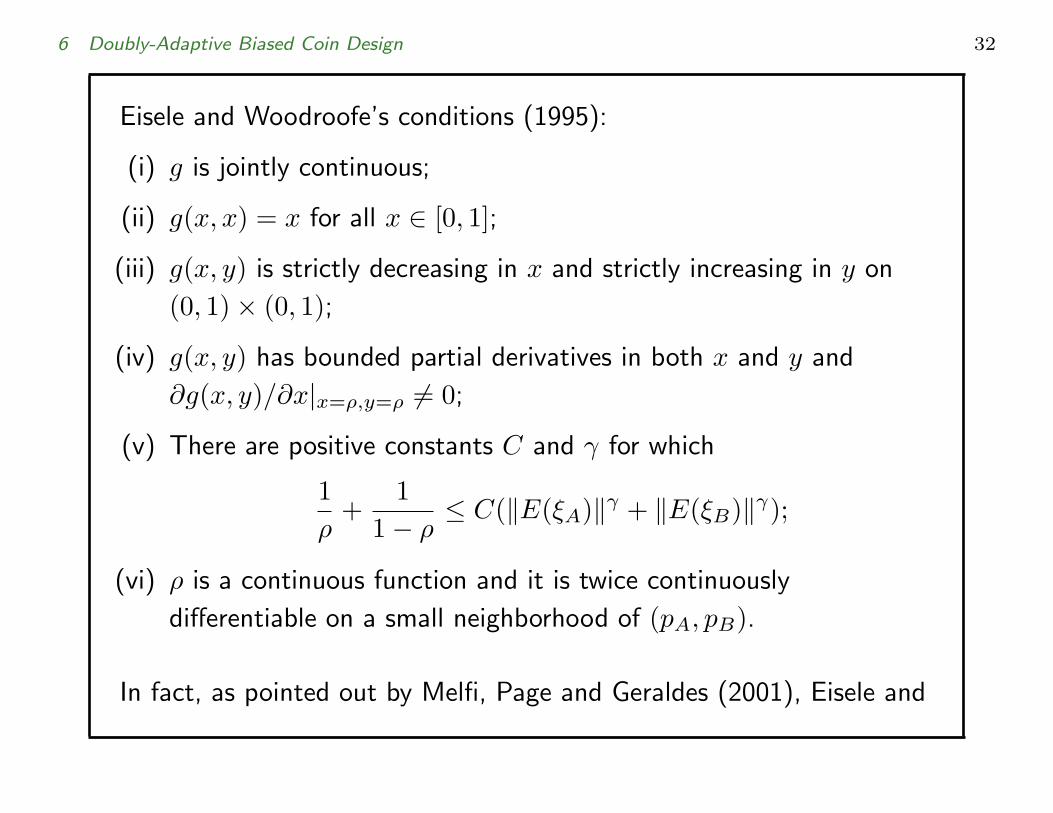
Eisele and Woodroofe’s conditions (1995):
(i) g is jointly continuous;
(ii) g(x, x) = x for all x ∈ [0, 1];
(iii) g(x, y) is strictly decreasing in x and strictly increasing in y on
(0, 1)× (0, 1);
(iv) g(x, y) has bounded partial derivatives in both x and y and
∂g(x, y)/∂x|x=ρ,y=ρ 6= 0;
(v) There are positive constants C and γ for which
1ρ
+1
1− ρ≤ C(‖E(ξA)‖γ + ‖E(ξB)‖γ);
(vi) ρ is a continuous function and it is twice continuously
differentiable on a small neighborhood of (pA, pB).
In fact, as pointed out by Melfi, Page and Geraldes (2001), Eisele and

6 Doubly-Adaptive Biased Coin Design 33
Woodroofe’s g(x, ρ) violated their regularity conditions (iv) and (v).
Recently, Hu and Zhang (2004) proposed (γ ≥ 0)
g(x, ρ) =ρ(ρ/x)γ
ρ(ρ/x)γ + (1− ρ)((1− ρ)/(1− x))γ
• γ = 0, the g(x, ρ) = ρ (the SMLE);
• γ = ∞, determined design.
(vii) There exists δ > 0, such that g(x, y) satisfies
g(x, y) = g(ρ, ρ) + (x− ρ)∂g
∂x|(ρ,ρ)
+(y − ρ)∂g
∂y|(ρ,ρ) + o(|x− ρ|1+δ) + o(|y − ρ|1+δ)
as (x, y) → (ρ, ρ).
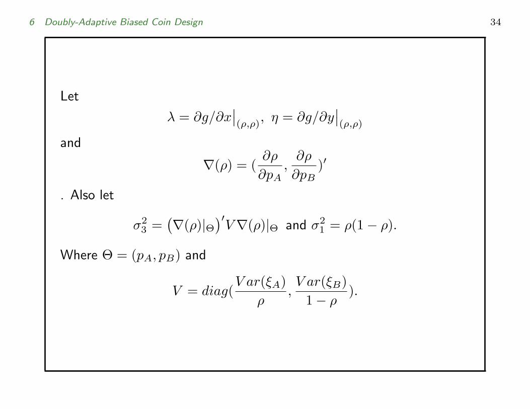
6 Doubly-Adaptive Biased Coin Design 34
Let
λ = ∂g/∂x∣∣(ρ,ρ)
, η = ∂g/∂y∣∣(ρ,ρ)
and
∇(ρ) = (∂ρ
∂pA,
∂ρ
∂pB)′
. Also let
σ23 =
(∇(ρ)|Θ
)′V∇(ρ)|Θ and σ2
1 = ρ(1− ρ).
Where Θ = (pA, pB) and
V = diag(V ar(ξA)
ρ,V ar(ξB)
1− ρ).
6 Doubly-Adaptive Biased Coin Design 35
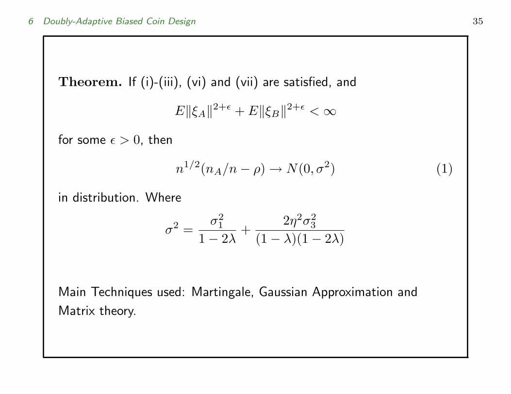
Theorem. If (i)-(iii), (vi) and (vii) are satisfied, and
E‖ξA‖2+ε + E‖ξB‖2+ε < ∞
for some ε > 0, then
n1/2(nA/n− ρ) → N(0, σ2) (1)
in distribution. Where
σ2 =σ2
1
1− 2λ+
2η2σ23
(1− λ)(1− 2λ)
Main Techniques used: Martingale, Gaussian Approximation and
Matrix theory.

6 Doubly-Adaptive Biased Coin Design 36
For binary responses with (ρ = qB/(qA + qB)),
n1/2(nA/n− ρ) → N(0, σ2DBCD)
in distribution, whenever λ < 1/2, where
σ2DBCD =
q1q2
(1− 2λ)(q1 + q2)2+
2η2
(1− λ)(1− 2λ)q1q2(p1 + p2)
(q1 + q2)3

6 Doubly-Adaptive Biased Coin Design 37
If
g(x, ρ) =ρ(ρ/x)γ
ρ(ρ/x)γ + (1− ρ)((1− ρ)/(1− x))γ,
then
σ2DBCD =
q1q2(p1 + p2)(q1 + q2)3
+2q1q2
(1 + 2γ)(q1 + q2)3.
• γ = 0, σ2DBCD = q1q2(p1+p2+2)
(q1+q2)3.
• γ = ∞, σ2DBCD = q1q2(p1+p2)
(q1+q2)3(Lower bound).
• γ = 2, σ2DBCD = q1q2(p1+p2+.4)
(q1+q2)3.

7 Some recent developments 38
7 Some recent developments
To compare different designs, it is important to obtain the asymptotic
distribution and asymptotic variance of nA/n.
• Generalized Friedman’s urn models (K treatments):
– Athreya and Karlin (1968, Annals of Mathematical Statistics)
obtained the consistent of nA/n; They conjectured the
asymptotic of nA/n.
– Bai and Hu (2005, Annals of Applied Probability) obtained the
asymptotic normality and asymptotic variance of nA/n.
– Zhang, Hu and Cheung (2006, Annals of Applied Probability)
proposed estimation-adjusted urn models that can target any
given allocation and also apply to different responses.
• Optimal allocation and implementing DBCD
– Two treatments: Binary responses (Rosenberger et al, 2001,
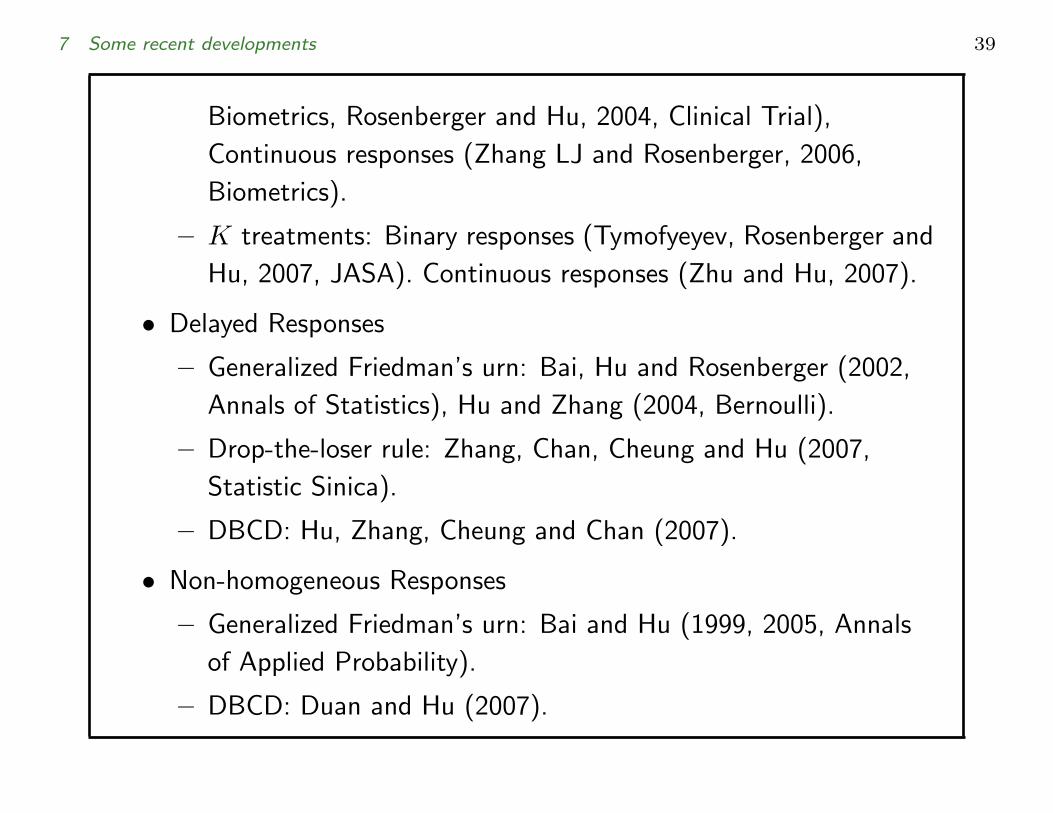
7 Some recent developments 39
Biometrics, Rosenberger and Hu, 2004, Clinical Trial),
Continuous responses (Zhang LJ and Rosenberger, 2006,
Biometrics).
– K treatments: Binary responses (Tymofyeyev, Rosenberger and
Hu, 2007, JASA). Continuous responses (Zhu and Hu, 2007).
• Delayed Responses
– Generalized Friedman’s urn: Bai, Hu and Rosenberger (2002,
Annals of Statistics), Hu and Zhang (2004, Bernoulli).
– Drop-the-loser rule: Zhang, Chan, Cheung and Hu (2007,
Statistic Sinica).
– DBCD: Hu, Zhang, Cheung and Chan (2007).
• Non-homogeneous Responses
– Generalized Friedman’s urn: Bai and Hu (1999, 2005, Annals
of Applied Probability).
– DBCD: Duan and Hu (2007).

8 Further Topics 40
8 Further Topics
• Sample size of randomized design.
– Power is a random variable (Hu (2004) for K = 2, two-arm
trials);
– For K > 2, unknown.
• Using covariate information in adaptive designs.
– Some preliminary results: Zhang, Hu, Cheung and Chan (2007,
Annals of Statistics) and Gwise’s Thesis;
– D-optimal designs (Gwise, Hu and Hu, 2006);
– A lot of research problems.
• Best adaptive randomizations.
– Fully randomized procedure (best) that targets any allocation?
Hu, Zhang and He (2007, Submitted)

8 Further Topics 41
– Best adaptive randomization for multi-arm trials.
• Fixing power and minimizing expected failures.
– Simulation studies of K = 2 (Rosenberger and Hu (2004,
Clinical Trial));
– General cases; unknown.
• Survival responses.
• Balance covariates in clinical trials.

9 Future of RAR 42
9 Future of RAR
• White Papers on Response-Adaptive Randomization for FDA
(2007).
• Adaptive Trials in the future (The Wall Street Journal, July 10,
2006).
• Hu and Rosenberger’s book: The Theory of Response Adaptive
Randomization in Clinical Trials, John Wiley, 2006.
• 63rd Deming Conference on Applied Statistics
(Bio-pharmaceutical Section of ASA). Over 100 Bio-statisticians
will attend the three hour session about RAR (Dec 4, 2007).

9 Future of RAR 43
Thank You!