resolution analysis in full waveform inversionfichtner/papers/2011_resolution.pdf · resolution in...

Geophys. J. Int. (2011) 187, 1604–1624 doi: 10.1111/j.1365-246X.2011.05218.x

Sei

smol

ogy

Resolution analysis in full waveform inversion

Andreas Fichtner and Jeannot TrampertDepartment of Earth Sciences, Utrecht University, Utrecht, the Netherlands. E-mail: [email protected]

Accepted 2011 September 5. Received 2011 July 12; in original form 2011 May 12

S U M M A R YWe propose a new method for the quantitative resolution analysis in full seismic waveforminversion that overcomes the limitations of classical synthetic inversions while being computa-tionally more efficient and applicable to any misfit measure. The method rests on (1) the localquadratic approximation of the misfit functional in the vicinity of an optimal earth model, (2)the parametrization of the Hessian in terms of a parent function and its successive derivativesand (3) the computation of the space-dependent parameters via Fourier transforms of theHessian, calculated with the help of adjoint techniques. In the simplest case of a Gaussianapproximation, we can infer rigorously defined 3-D distributions of direction-dependent res-olution lengths and the image distortion introduced by the tomographic method. We illustratethese concepts with a realistic full waveform inversion for upper-mantle structure beneath Eu-rope. As a corollary to the method for resolution analysis, we propose several improvements tofull waveform inversion techniques. These include a pre-conditioner for optimization schemesof the conjugate-gradient type, a new family of Newton-like methods, an approach to adaptiveparametrization independent from ray theory and a strategy for objective functional designthat aims at maximizing resolution. The computational requirements of our approach are lessthan for a typical synthetic inversion, but yield a much more complete picture of resolution andtrade-offs. While the examples presented in this paper are rather specific, the underlying ideais very general. It allows for problem-dependent variations of the theme and for adaptationsto exploration scenarios and other wave-equation-based tomography techniques that employ,for instance, georadar or microwave data.

Key words: Fourier analysis; Inverse theory; Seismic tomography; Computational seismol-ogy; Theoretical seismology; Wave propagation.

1 I N T RO D U C T I O N

Full waveform inversion is a tomographic technique that is based on numerical wave propagation through complex media combined withadjoint or scattering integral methods for the computation of Frechet kernels. The accurate and complete solution of the seismic wave equationensures that information from the full seismogram can be used for the purpose of improved tomographic models. Originally conceived inthe late 1970s and early 1980s (Bamberger et al. 1977, 1982; Tarantola 1984), realistic applications have become feasible only recently.Full waveform inversion can now be used to solve local-scale engineering and exploration problems (e.g. Smithyman et al. 2009; TakamTakougang & Calvert 2011), to study crustal-scale deformation processes (e.g. Bleibinhaus et al. 2007; Chen et al. 2007; Tape et al. 2009),to reveal the detailed structure of the lower mantle (e.g. Konishi et al. 2009; Kawai & Geller 2010) or to refine continental-scale models fortectonic interpretations and improved tsunami warnings (e.g. Fichtner et al. 2010; Hingee et al. 2011). While the tomographic method itselfhas advanced substantially, an essential aspect of the inverse problem has been ignored almost completely, despite its obvious socio-economicrelevance: the quantification of resolution and uncertainties.

1.1 Resolution analysis in full waveform inversion

Early attempts to analyse—and in fact define—resolution were founded on the equivalence of diffraction tomography and the first iterationof a full waveform inversion (e.g. Devaney 1984; Wu & Toksoz 1987; Mora 1989). This equivalence, however, holds only in the impracticalcase where the misfit χ is equal to the L2 waveform difference. Furthermore, the rigorous analysis of diffraction tomography is restrictedto homogeneous or layered acoustic media. The resulting resolution estimates are too optimistic for realistic applications that suffer frommodelling errors and the sparsity of noisy data (Bleibinhaus et al. 2009).

Re-use of this article is permitted in accordance with the Terms and Conditions set out at http://wileyonlinelibrary.com/onlineopen#OnlineOpen_Terms

1604 C© 2011 The Authors

Geophysical Journal International C© 2011 RAS

Geophysical Journal International

Resolution in full waveform inversion 1605

Resolution analysis in full waveform inversion is complicated by many factors: (1) The data depend non-linearly on the model,meaning that the well-established machinery of linear inverse theory is not applicable (Backus & Gilbert 1967; Tarantola 2005). (2) A directconsequence of non-linearity is the appearance of multiple local minima (e.g. Gauthier et al. 1986). These may be avoided with the helpof various multiscale approaches (e.g. Bunks et al. 1995; Sirgue & Pratt 2004; Ravaut et al. 2004; Fichtner et al. 2009), also known asfrequency-hopping in the microwave imaging literature (e.g. Chew & Lin 1995). The convergence of all currently used multiscale approachesis, however, purely empirical. (3) Contrary to most linearized tomographies, the sensitivity matrix is not computed explicitly in full waveforminversion for reasons of numerical efficiency. This prevents a local analysis based, for instance, on the computation of the resolution andcovariance operators for large linear systems (Nolet et al. 1999; Boschi 2003). (4) The size of the model space and the costs of the forwardproblem solution prohibit the application of probabilistic approaches that account for non-linearity using Monte Carlo sampling (Sambridge& Mosegaard 2002; Tarantola 2005) or neural networks (Devilee et al. 1999; Meier et al. 2007a,b).

In the absence of a quantitative means to assess resolution, arguments concerning the reliability of full waveform inversion images aremostly restricted to synthetic inversions for specific input structures, on the visual inspection of the tomographic images or on the analysisof the data fit. Synthetic inversions are known to be potentially misleading even in linearized tomographies (Leveque et al. 1993). Visualinspection is equally inadequate because the appearance of small-scale heterogeneities is too easily mistaken as an indicator of high resolution.Finally, a good fit between observed and synthetic waveforms merely proves that the tomographic system has been solved, but not necessarilyresolved.

Despite being crucial for the interpretation of the tomographic images, methods for the quantification of resolution in realistic applicationsof full waveform inversion do not exist so far. This deficiency is the source of much scepticism as to whether it is really worth the effort.

Despite the difficulties introduced by the non-linearity of full waveform inversion combined with the computational costs of the forwardproblem solution, ample information about local resolution can be inferred from the quadratic approximation of the misfit functional χ .

χ (m) = χ (m) + 1

2

∫G

∫G

[m(x) − m(x)]T H(x, y) [m(y) − m(y)] d3x d3y , (1)

where

m(x) = [m1(x), m2(x), . . . , m N (x)]T (2)

represents an earth model composed of N physical quantities. The components of m may, for instance, be the P velocity α, the S velocity β

and density ρ, that is, (m1, m2, m3)T = (α, β, ρ)T . The optimal earth model m is characterized by a zero Frechet derivative, meaning that

∇mχ (m) δm = limε→0

1

ε[χ (m + ε δm) − χ (m)] = 0 (3)

for all model perturbations δm. The Hessian H is a symmetric and bilinear operator that acts on the perturbation δm = m − m via a doubleintegral over the model volume G.

1.2 The role of the Hessian in resolution analysis

The importance of the Hessian in local resolution analysis arises directly from the second-order approximation (1) but also from its relationsto the posterior covariance, extremal bounds analysis and point-spread functions (PSFs).

1.2.1 Inferences on resolution and trade-offs from the local approximation

Locally, that is, in the vicinity of the optimum m, the Hessian describes the geometry of χ in terms of its curvature or convexity. In thissense, H provides the most direct measure of resolution and trade-offs as it describes the change of the misfit when m is slightly perturbedto m + δm. The diagonal element Hii (x, x) defines the local resolution of the model parameter mi at position x. The off-diagonal elementsHi j (x, x)|i �= j measure the trade-offs between mi and model parameters mj|j �=i at position x, that is the extent to which the model parametersare dependent. Similarly, the off-diagonal elements Hi j (x, y)|x�=y encapsulate spatial dependencies between model parameters mi and mj atdifferent positions x and y. Large off-diagonal elements imply that simultaneous perturbations of different parameters or in different regionscan compensate each other, to leave the misfit χ nearly unchanged.

1.2.2 Relation of the Hessian to the posterior covariance

A further interpretation of the Hessian is related to Bayesian inference (e.g. Jaynes 2003; Tarantola 2005) where the available information ona model m is expressed in terms of a probability density σ (m). In the specific case of a linear forward problem and Gaussian distributionsdescribing prior knowledge and measurement errors, σ (m) takes the form

σ (m) = const. e−χg (m) (4)

with the misfit functional

χg(m) = 1

2

∫G

∫G

[m(x) − m(x)]T S−1(x, y) [m(y) − m(y)] d3x d3y (5)

C© 2011 The Authors, GJI, 187, 1604–1624


1606 A. Fichtner and J. Trampert

and the posterior covariance S. The comparison between (5) and the quadratic approximation (1) suggests the interpretation of H in terms ofthe inverse posterior covariance in a local probabilistic sense.

1.2.3 Extremal bounds analysis

In addition to being the carrier of covariance information, the Hessian H provides the extremal bounds within which the optimal model mcan be perturbed without increasing the misfit χ (m) beyond a pre-defined limit χ (m) + δχ , where δχ is usually related to the noise in thedata (Meju & Sakkas 2007; Meju 2009). The model mextr that extremizes the integral of the model parameter mi over a specific region Gδ⊂G,that is,

∫Gδ

mi (x) d3x, while increasing the misfit to χ (m) + δχ , is given by (Fichtner 2010)

mextrj (x) = m j (x) − λ

∫Gδ

H−1i j (x, y) d3y with λ = ±(2δχ )1/2

[∫Gδ

∫Gδ

H−1i i (x, y) d3x d3y

]−1/2

(6)

and no summation over the repeated indices ii. Eq. (6) involves the inverse Hessian H−1, interpreted already in terms of the local posteriorcovariance. Extremal bounds analysis therefore attaches a deterministic and quantitative meaning to an originally probabilistic concept. Largevariances H−1

ii imply that large perturbations of parameter mi within the region Gδ do not increase the misfit beyond the admissible bound δχ ,meaning that mi is poorly constrained inside Gδ . The presence of non-zero covariances H−1

ij |j �=i indicates that joint perturbations of all modelparameters compensate each other, to allow for even larger perturbations of the parameter mi that we wish to extremize in the above-mentionedsense.

1.2.4 Point-spread functions

Finally, we can relate the Hessian to PSFs or spike tests that are commonly used as a diagnostic tool for resolution and trade-offs in linearizedtomographic problems (e.g. Spakman 1991; Zielhuis & Nolet 1994; Yu et al. 2002; Fang et al. 2010). For this, we consider a special type ofsynthetic inversion where the initial model m(0)(y) is nearly equal to the optimal model m(y). The only deficiency of m(0)(y) is the absenceof a point perturbation of parameter mi that is point-localized at position x, that is,

m(0)(y) = m(y) − δm(y) = m(y) −

⎡⎢⎣ 0︸︷︷︸δm1

, . . . , 0︸︷︷︸δmi−1

, δ(y − x)︸︷︷︸δmi

, 0︸︷︷︸δmi+1

, . . . , 0︸︷︷︸δm N

⎤⎥⎦T

. (7)

Using the quadratic approximation (1) and the definition of the Frechet derivative (3), we find that the j-component of the Frechet derivative∇mχ evaluated at the initial model m(0), that is, ∇mχ

(0)j (x), is given by

∇mχ(0)j (x) =

∫G

[m(0)

k (x′) − mk(x′)]

Hkj (x′, y) d3x′ = −

∫G

δmk(x′) Hkj (x′, y) d3x′ = −Hi j (x, y) , (8)

where the summation over repeated indices is implicitly assumed from hereon. The first iteration of a gradient-based optimization schemewould then update m(0)(x) to an improved model m(1) ≈ m, the components of which are given by

m(1)j (x) = m(0)

j (x) − γ ∇mχ(0)j (x) = m(0)

j (x) + γ Hi j (x, y) . (9)

The scalar γ is the step length that minimizes χ along the local direction of steepest descent, −∇mχ (0)(x). Eq. (9) reveals that the HessianH(x, y) represents our blurred perception of a point-localized perturbation at position y in a linearized tomographic inversion. The effect ofthe off-diagonal elements Hij|i �=j is to introduce unwanted updates of model parameters mj|i �=j that have initially not been perturbed.

In the restricted sense of eq. (9), the Hessian Hi j (x, y) is the PSF, that is, the response of model parameter mj to a linearized spiketest with a point perturbation of mi at position x. A fully non-linear spike test based on gradient optimization with multiple iterations willgenerally lead to a sharper reconstruction of the input spike, so that H(x, y) can be considered a conservative estimate of the non-linearPSF. Throughout the following developments, we use the term PSF in the linearized sense as a synonym for the Hessian because it offers anintuitive interpretation of H(x, y). Although the significance of the Hessian in local resolution analysis is evident, the efficient computationof H in time-domain modelling of seismic wave propagation remains challenging. The most efficient approach involves a modification of thewell-known adjoint method (e.g. Tarantola 1988; Tromp et al. 2005; Fichtner et al. 2006; Liu & Tromp 2006; Plessix 2006; Chen 2011) thatallows us to compute H applied to a model perturbation δm, that is,∫

GH(x, y) δm(y) d3y (10)

using two forward and two adjoint simulations, as described in Santosa & Symes (1988), Fichtner & Trampert (2011) and Appendix A.A model perturbation δm samples the Hessian via the integral (10); and by sampling H with a suitable set of model perturbations, we

can gather as much second-derivative information as needed for our purposes, though at the expense of potentially prohibitive computationalrequirements. It is therefore the purpose of this paper to develop a sampling strategy of the Hessian that operates with as few modelperturbations as possible while leading to an approximation of H that is physically meaningful and interpretable.

C© 2011 The Authors, GJI, 187, 1604–1624



1.3 Outlook

This paper is organized as follows: We start in Section 2 with a brief description of a full waveform inversion for upper-mantle structurebeneath Europe that will serve as both motivation and testing ground for the subsequent developments. In Section 3, we approximate theHessian by a position-dependent Gaussian, the parameters of which can be computed efficiently via the Fourier transform of H(x, y) for asmall set of wavenumber vectors. The Gaussian approximation can be generalized with the help of Gram–Charlier expansions that expressH(x, y) in terms of a parent function and its successive derivatives. Following the theoretical developments, we demonstrate in Section 4how the Gaussian approximation of the Hessian can be used to infer the image distortion introduced by the tomographic method, as wellas the distribution of direction-dependent resolution lengths. Section 5 provides an intuitive interpretation of the physics behind the Fouriertransformed Hessian. This interpretation partly motivates several improvements to full waveform inversion techniques proposed in Section 6.These include a new family of Newton-like methods, a pre-conditioner for gradient methods, an approach to adaptive parametrizationindependent from ray theory and a criterion for the design of misfit functionals aiming at maximum resolution. Finally, in Appendices A andB, we review the computation of Hessian kernels and multidimensional Gram–Charlier expansions.

2 T H E T E S T I N G G RO U N D : A R E A L I S T I C F U L L WAV E F O R M I N V E R S I O N

To illustrate the theoretical developments of the following sections with practical applications, we consider a long-wavelength full waveforminversion for European upper-mantle structure (Fig. 1). While this example is very specific, all subsequent developments are valid also forsmaller scale applications, for instance, in the context of active source exploration and engineering problems.

As data we used 2200 mostly vertical-component seismograms from 40 events that occurred in Europe and western Asia between 2002and 2010. To quantify the discrepancies between observed and synthetic waveforms, we measured time- and frequency-dependent phasemisfits within a period band from 100 to 300 s (Fichtner et al. 2009). In addition to surface waves, we also included long-period body wavesand unidentified phases. The numerical modelling was based on a spectral-element discretization of the seismic wave equation, as describedin Fichtner & Igel (2008).

To ensure the rapid convergence of the iterative misfit minimization, we implemented a 3-D initial model. The initial crustal structureis a long-wavelength equivalent (Fichtner & Igel 2008) of the maximum likelihood model of Meier et al. (2007a,b)) who inverted surfacewave dispersion for crustal thickness and the isotropic S velocity β. Within the continental crust, the isotropic P wave speed α, and densityρ, are scaled to β as α = 1.5399β + 840 m s−1, and ρ = 0.2277β + 2016 kg m−3(Meier et al. 2007a). Velocities and density within theoceanic crust are fixed to the values of crust 2.0 (Bassin et al. 2000). As 3-D initial mantle structure we use the isotropic S velocity variationsof model S20RTS (Ritsema et al. 1999) added to an isotropic version of the 1-D model PREM (Dziewonski & Anderson 1981) where the220 km discontinuity has been replaced by a linear gradient. The scaling to α is depth-dependent, as inferred from P, PP, PPP and PKPtraveltimes (Ritsema & van Heijst 2002). The initial density structure in the mantle is radially symmetric.

During the inversion, we successively update both β and α, as well as ρ. After seven conjugate-gradient iterations, the total misfitreduction reached nearly 50 per cent, whereas it was below 2 per cent for the seventh iteration alone. This indicates that the final model, shownin Fig. 1(b), is indeed close to the optimum. Despite being computed from long-period data, the model clearly reveals prominent featurespreviously imaged in both body and surface wave tomographic studies (e.g. Spakman 1991; Zielhuis & Nolet 1994; Boschi et al. 2004; Peteret al. 2008; Schivardi & Morelli 2011; Schafer et al. 2011). These include the low velocities beneath the Iceland hotspot and the westernMediterranean Basin, the slow-to-fast transition from Phanerozoic central Europe to the Precambrian east European platform, and the highvelocities beneath the Hellenic arc.

Having reached a nearly optimal model, we can compute the PSF, H(x, y), in the sense of Section 1.2.4. The result for a point-localizedS velocity perturbation at 180 km below northern Germany is shown in Fig. 2.

Figure 1. (a) Distribution of earthquakes (blue dots) and stations (red dots). Black lines represent the central segments of surface wave ray paths. (b) Horizontalslices through the S velocity model at 100 and 200 km depth.

C© 2011 The Authors, GJI, 187, 1604–1624



Figure 2. Horizontal (top) and vertical (below) slices through different components of the PSF H(x, y), for a fixed x at 180 km depth below northern Germany.The free space variable is y. (a) The ββ-component of the Hessian, Hββ (x, y), that corresponds to a point-localized S velocity perturbation at x. Solid anddashed red lines indicate the position of x. Note that the colour scale is chosen such that negative values are emphasized. (b) The same as to the left, but for theβα-component of the PSF, Hβα(x, y). The amplitude of the horizontal slice at 180 km depth is multiplied by 20 to enhance visibility. The colour scale is againadapted to emphasise negative values. (c) Slices through the βρ-component of the Hessian, Hβρ (x, y). Note the condensed colour scale and the appearance ofstrong negative values near the surface.

The spatial extent of the ββ-component Hββ (x, y), displayed in Fig. 2(a), describes the trade-offs between an S velocity perturbationlocated at position x, and the S velocity in the surrounding model volume. With few exceptions, Hββ (x, y) is positive, meaning that negativeperturbations in β compensate positive ones, and vice versa. The black and grey-shaded volume where trade-offs between S velocityperturbations are most significant, is roughly N-S oriented with a weak tail extending beneath Scandinavia and the North Atlantic. Interpretedin terms of a PSF, the Hessian component Hββ (x, y) is the S velocity structure recovered in a single-iteration synthetic inversion wherethe input was a perturbation in β localized at position x. The width of the PSF loosely defines a resolution length within which S velocityperturbations cannot be constrained independently. We will return to the resolution length concept in Section 4.

Fig. 2(b) shows the βα-component of the Hessian, Hβα(x, y), which represents the trade-offs between P and S velocity perturbations.While the horizontal slice qualitatively resembles Hββ (x, y), the vertical slices reveal that trade-offs between α and β are restricted to shallowdepths of less than 50 km. This was to be expected because our data set is dominated by Rayleigh waves that are affected by P velocitystructure only near the surface.

The βρ-component Hβρ(x, y), visualized in Fig. 2(c), reveals a surprising complexity that is reminiscent of the strongly oscillatorydensity kernels for Rayleigh waves (e.g. Takeuchi & Saito 1972; Cara et al. 1984). The absolute values of Hβρ(x, y) are generally smallcompared to those of the other components, meaning that the trade-offs between S velocity and density are hardly significant.

In general, the details of the PSFs depend on both the data and the position of the point perturbation relative to sources and receivers.However, from a series of numerical experiments, we conclude that several characteristics of the PSFs are position-independent. These includethe comparatively small amplitude of Hβρ , the restriction of Hβα to shallow depths and the roughly bell-shaped geometry of Hββ .

3 F O U R I E R - D O M A I N A P P ROX I M AT I O N O F T H E H E S S I A N - I : T H E O RY

To fully quantify resolution and trade-offs, PSFs should ideally be computed for every model parameter and for every point x within thevolume of interest. Since the resulting computational costs would clearly be prohibitive, we propose an efficient scheme for the approximationof PSFs. This is based on a parametrization of the Hessian, followed by the estimation of the space-dependent parameters with the help ofFourier transforms.

C© 2011 The Authors, GJI, 187, 1604–1624



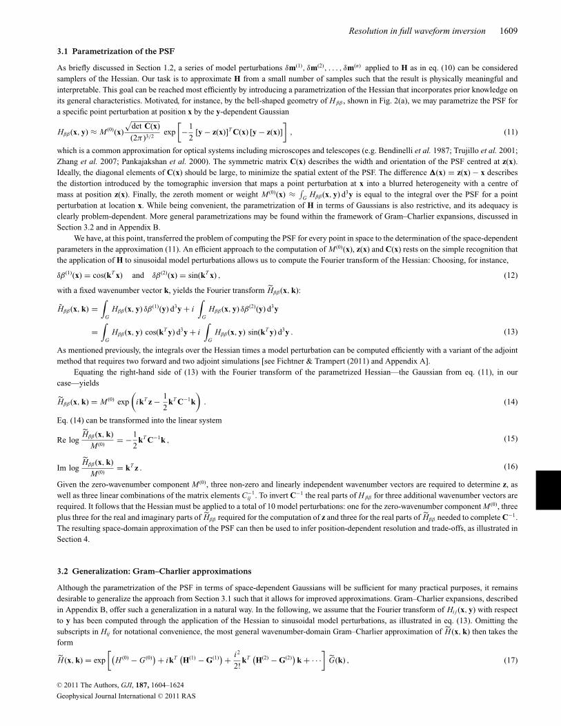
3.1 Parametrization of the PSF

As briefly discussed in Section 1.2, a series of model perturbations δm(1), δm(2), . . . , δm(n) applied to H as in eq. (10) can be consideredsamplers of the Hessian. Our task is to approximate H from a small number of samples such that the result is physically meaningful andinterpretable. This goal can be reached most efficiently by introducing a parametrization of the Hessian that incorporates prior knowledge onits general characteristics. Motivated, for instance, by the bell-shaped geometry of Hββ , shown in Fig. 2(a), we may parametrize the PSF fora specific point perturbation at position x by the y-dependent Gaussian

Hββ (x, y) ≈ M (0)(x)

√det C(x)

(2π )3/2exp

[−1

2[y − z(x)]T C(x) [y − z(x)]

], (11)

which is a common approximation for optical systems including microscopes and telescopes (e.g. Bendinelli et al. 1987; Trujillo et al. 2001;Zhang et al. 2007; Pankajakshan et al. 2000). The symmetric matrix C(x) describes the width and orientation of the PSF centred at z(x).Ideally, the diagonal elements of C(x) should be large, to minimize the spatial extent of the PSF. The difference �(x) = z(x) − x describesthe distortion introduced by the tomographic inversion that maps a point perturbation at x into a blurred heterogeneity with a centre ofmass at position z(x). Finally, the zeroth moment or weight M (0)(x) ≈ ∫

G Hββ (x, y) d3y is equal to the integral over the PSF for a pointperturbation at location x. While being convenient, the parametrization of H in terms of Gaussians is also restrictive, and its adequacy isclearly problem-dependent. More general parametrizations may be found within the framework of Gram–Charlier expansions, discussed inSection 3.2 and in Appendix B.

We have, at this point, transferred the problem of computing the PSF for every point in space to the determination of the space-dependentparameters in the approximation (11). An efficient approach to the computation of M (0)(x), z(x) and C(x) rests on the simple recognition thatthe application of H to sinusoidal model perturbations allows us to compute the Fourier transform of the Hessian: Choosing, for instance,

δβ (1)(x) = cos(kT x) and δβ (2)(x) = sin(kT x) , (12)

with a fixed wavenumber vector k, yields the Fourier transform Hββ (x, k):

Hββ (x, k) =∫

GHββ (x, y) δβ (1)(y) d3y + i

∫G

Hββ (x, y) δβ (2)(y) d3y

=∫

GHββ (x, y) cos(kT y) d3y + i

∫G

Hββ (x, y) sin(kT y) d3y . (13)

As mentioned previously, the integrals over the Hessian times a model perturbation can be computed efficiently with a variant of the adjointmethod that requires two forward and two adjoint simulations [see Fichtner & Trampert (2011) and Appendix A].

Equating the right-hand side of (13) with the Fourier transform of the parametrized Hessian—the Gaussian from eq. (11), in ourcase—yields

Hββ (x, k) = M (0) exp

(ikT z − 1

2kT C−1k

). (14)

Eq. (14) can be transformed into the linear system

Re logHββ (x, k)

M (0)= −1

2kT C−1k , (15)

Im logHββ (x, k)

M (0)= kT z . (16)

Given the zero-wavenumber component M (0), three non-zero and linearly independent wavenumber vectors are required to determine z, aswell as three linear combinations of the matrix elements C−1

ij . To invert C−1 the real parts of Hββ for three additional wavenumber vectors arerequired. It follows that the Hessian must be applied to a total of 10 model perturbations: one for the zero-wavenumber component M (0), threeplus three for the real and imaginary parts of Hββ required for the computation of z and three for the real parts of Hββ needed to complete C−1.The resulting space-domain approximation of the PSF can then be used to infer position-dependent resolution and trade-offs, as illustrated inSection 4.

3.2 Generalization: Gram–Charlier approximations

Although the parametrization of the PSF in terms of space-dependent Gaussians will be sufficient for many practical purposes, it remainsdesirable to generalize the approach from Section 3.1 such that it allows for improved approximations. Gram–Charlier expansions, describedin Appendix B, offer such a generalization in a natural way. In the following, we assume that the Fourier transform of Hi j (x, y) with respectto y has been computed through the application of the Hessian to sinusoidal model perturbations, as illustrated in eq. (13). Omitting thesubscripts in Hij for notational convenience, the most general wavenumber-domain Gram–Charlier approximation of H (x, k) then takes theform

H (x, k) = exp

[(H (0) − G(0)

) + ikT(H(1) − G(1)

) + i2

2!kT

(H(2) − G(2)

)k + · · ·

]G(k) , (17)

C© 2011 The Authors, GJI, 187, 1604–1624



where G is the Fourier transform of a parent function G, and H(i)(x) and G(i)(x) are the position-dependent cumulants of H and G, alsointroduced in Appendix B. The first three cumulants of H (x, y) for a fixed value of x are related to the moments

M (n)i jk... =

∫R3

(yi y j yk . . .) H (x, y) d3y (18)

via

H (0) = log M (0) , H (1)i = M (1)

i

M (0), H (2)

i j = 1

M (0)

(M (2)

i j − M (1)i M (1)

j

M (0)

). (19)

Similar relations hold for the cumulants and moments of the parent function G. The first and second cumulants, H(1) and H(2), are the centreof mass and the inverse covariance of H (x, y)|x=const., respectively.

To allow for a good approximation with few coefficients, the parent function is usually chosen to have the same general characteristicsas the function that we wish to expand. Assuming, for instance, that H (x, y)|x=const. is roughly bell-shaped, as the PSF in Fig. 2(a), we canchoose the space-domain parent function to be the normalized Gaussian

G(y) =√

det C

(2π )3/2exp

[−1

2(y − z)T C (y − z)

](20)

with the x-dependent cumulants

G(0) = 0 , G(1) = z , G(2) = C−1 , G(n>2) = 0 . (21)

Since the values of the first and second cumulants are still undetermined at this point of the development, we are free to impose G(1) = H(1)

and G(2) = H(2), so that (17) reduces to the classical Gram–Charlier A series (e.g. Samuelson 1943; Cramer 1957)

H (x, k) = M (0) exp

[i3

3!H (3)

i jk ki k j kk + i4

4!H (4)

i jkl ki k j kkkl + . . .

]exp

(ikT z − 1

2kT C−1k

). (22)

Eq. (17) and its specialized form (22) are general expansions of the PSF in terms of its cumulants. The Gaussian parametrization fromSection 3.1 is, in this sense, a first-order or low-wavenumber approximation. Higher order terms in the Gram–Charlier series involve highercumulants and account for the shorter wavelength variations of the PSF.

Similar to the first-order approximation of eq. (14), the coefficients of a general Gram–Charlier expansions can be computed from theFourier transforms for sufficiently many independent wavenumber vectors k. The space-domain approximation corresponding to (22) is givenby (see Appendix B)

H (x, y) = M (0)

√det C

(2π )N/2

[1 + (−1)3

3!H (3)

i jk

∂

∂yi

∂

∂y j

∂

∂yk+ (−1)4

4!H (4)

i jkl

∂

∂yi

∂

∂y j

∂

∂yk

∂

∂yl+ · · ·

]exp

[−1

2(y − z)T C (y − z)

]. (23)

While the expansions (17) and (23) are very general, their physical interpretation is complicated by their complexity. We will therefore adhereto the low-wavenumber Gaussian approximation from Section 3.1 throughout the following examples.

4 F O U R I E R - D O M A I N A P P ROX I M AT I O N O F T H E H E S S I A N - I I : A P P L I C AT I O N

To make the previous developments explicit, we return to the full waveform inversion example introduced in Section 2. As a preparatory stepwe subdivide the study region into nearly equal volume blocks, shown in Fig. 3. These introduce a coordinate system that is approximatelycartesian over the expected width of the PSFs. The blocks, also used to parametrize the tomographic model from Fig. 1, are 1◦ × 1◦ wide and10 km deep. We then adopt the Gaussian parametrization of Hββ , proposed in eq. 11.

Figure 3. (Left) Subdivision of the model volume into blocks that are 1◦ × 1◦ wide and 10 km deep. The blocks introduce a coordinate system that is nearlycartesian over the width of the PSFs. (Right) The blocks are used also to parametrize the tomographic model. This figure shows a small part of the S velocitymodel from Fig. 1 at 100 km depth. Superimposed are the local coordinate lines that define the boundaries of the blocks. Arrows indicate the local x- andy-directions.

C© 2011 The Authors, GJI, 187, 1604–1624



Figure 4. (a) The zero-wavenumber perturbation δβ(k = 0) is equal to 1 m s−1 throughout the model volume. (b) Horizontal slices at 100 km, 200 km and300 km depth through the Fourier transform of the Hessian at zero wavenumber, Hββ (x, k = 0).

4.1 The zero-wavenumber component: relative weight of PSFs

We obtain the Fourier transform at zero wavenumber, Hββ (x, k = 0), from the application of Hββ (x, y) to an S velocity perturbation δβ(x)that is constant throughout the model volume, as shown in Fig. 4(a). The result is—irrespective of any parametrization or approximation—thespace-dependent zeroth moment

M (0)(x) = Hββ (x, k = 0) =∫

GHββ (x, y) d3y . (24)

Horizontal slices though M (0)(x) at 100, 200 and 300 km depth are displayed in Fig. 4(b). As expected, the zeroth moment is mostly positive,with few exceptions at shallow depth confined to the immediate vicinity of sources or receivers. Clearly visible are diffuse versions of raybundles that connect the epicentres along the periphery of the European plate to those regions with the highest station density. Furthermore,the zeroth moment decreases with depth below 200 km, as expected for a surface wave dominated data set.

According to eq. (24), the zeroth moment is equal to the integral over the PSF for a point perturbation at position x. It follows thatM (0)(x) is small when the misfit χ is nearly unaffected by a point perturbation at x. In contrast, M (0)(x) is large when the PSF has a highamplitude, a large spatial extent, or both. In this sense, the spatial variability of M (0)(x) reflects the relative weight of neighbouring PSFs.Information on the resolution length is not contained in the zeroth moment.

From the perspective of gradient-based optimization, M (0)(x) is proportional to the direction of steepest descent evaluated at a modelm + δm that differs from the optimal model m by a constant S velocity perturbation. In the case of perfect data coverage, we would thereforeexpect M (0)(x) to be constant throughout the model volume. The obvious departures from this ideal scenario, seen in Fig. 4(b), result fromthe limited sensitivity to deep structure in a surface wave dominated tomography, and from the clustering of sources and receivers. Theseclusters dominate the misfit, which then leads to a heterogeneous direction of steepest descent.

4.2 Real and imaginary parts of the Fourier transform: image distortion

Tomographic inversions map point perturbations into blurred versions of themselves. The centre of mass of the blurred image—that is theposition where the heterogeneity is visually perceived—does not generally coincide with the location of the original point perturbation. Thisdistortion can be quantified, at least in a linearized sense, using the approach described in Section 3.

Based on eq. (12), we compute the spectrum Hββ (x, k) for a non-zero wavenumber k by applying the Hessian Hββ (x, y) to the sinusoidalmodel perturbations δβ(x) = cos(kT x) and δβ(x) = sin(kT x). For our example, we choose the wavelength of the oscillations to be 2000 km.The model perturbations together with the real and imaginary parts of Hββ (x, k) are shown in Fig. 5 for a wavenumber vector pointing in thex-direction of the coordinate system introduced in Fig. 3 (nearly N–S in geographic coordinates).

Both the real and imaginary parts reveal a similar oscillatory pattern as the sinusoidal model perturbations from which they originate.This behaviour is to be expected provided that any PSF is roughly a space-shifted version of the PSF for a perturbation at the coordinateorigin x = 0, that is, Hββ (x, y) ≈ Hββ (0, y − x). Deviations from exact sinusoidal oscillations therefore reflect the spatially variable shapeand amplitude of the PSFs.

When interpreted within the framework of the Gaussian approximation (eqs 11 and 14), we can use the spectrum from Fig. 5 to computethe distortion

�(x) = z(x) − x (25)

which is the distance between a point-localized perturbation at position x, and the centre of mass of the corresponding PSF, z(x). The distortionmeasures the displacement of a point perturbation caused by the tomographic inversion. Upon inserting the definition (25) into eq. (14), we

C© 2011 The Authors, GJI, 187, 1604–1624



Figure 5. Horizontal slices through the sinusoidal model perturbations and the corresponding real and imaginary parts of Hββ (x, k). The black curves in thespectral maps delineate the zero lines in the model perturbations and are intended to guide the eye.

Figure 6. (a) The lateral component of the distortion �(x) at 100 and 200 km depth, respectively. The length of the red line in the figure headings is the scalefor the length of the arrows. (b) Surface projections of the central segments of the ray paths connecting sources (blue dots) to receivers (red dots).

obtain

Hββ (x, k) exp(−ikT x

) = M (0) exp(i kT �

)exp

(−1

2kT C−1k

). (26)

The three components of the distortion � can then be obtained from the evaluation of eq. (26) for three linearly independent wavenumbervectors. We note that the calculation of the complex argument kT � needs regularized because phase jumps appear where |Hββ (x, k)| is small.This regularization can be achieved by adding a constant ε > 0 to the real part of (26), so that kT � is forced to zero as |Hββ (x, k)| dropsbelow ε.

The lateral distortion, that is, the horizontal component of �, computed from the spectra for two linearly independent wavenumbervectors, is shown in Fig. 6. The interpretation must account for the regularization, which in this particular case means that � is stronglyattenuated in regions where the absolute value of the spectrum shown in Fig. 5 drops below 0.5 × 10−15 rad s m−4. Loosely speaking, thedistortion is meaningful only in regions where the PSFs are significantly non-zero.

Throughout central Europe, the lateral distortion is below 300 km, which is due to the high station density. Large distortions appear tobe rather localized, for instance, east of the Caspian Sea where ray paths are almost exclusively N–S oriented. As intuitively expected, �

slightly increases with increasing depth.

4.3 Resolution lengths

One of the most relevant quantities to be considered in resolution analysis is the resolution length, that is, the distance within which two pointperturbations cannot be constrained independently.

The resolution length is the direction-dependent extent of the PSF that defines a region where the original point perturbation trades offsignificantly with neighbouring heterogeneities. Within the Gaussian approximation (11), the width of a PSF is controlled by the positivedefinite matrix C(x), the inverse of which can be estimated from the spectrum (14).

We use the standard deviation of the Gaussian in a direction specified by the unit vector e,

e = 1√eT C e

, (27)

C© 2011 The Authors, GJI, 187, 1604–1624



Figure 7. Horizontal slices at 100 and 200 km depth through the resolution length distributions in the directions indicated by the arrows. (a) x-direction of thelocal coordinate system from Fig. 3 (roughly N–S in central and western Europe). (b) y-direction of the local coordinate system from Fig. 3 (roughly E–W incentral and western Europe).

as our definition of the direction-dependent resolution length. This means in the context of our specific example that S velocity perturbationsseparated by less than the resolution length effectively appear as one heterogeneity, instead of having clearly separate identities.

Distributions of horizontal resolution lengths in two perpendicular directions are shown in Fig. 7. The resolution length in x-direction(nearly N–S in central and western Europe) reaches its minimum of 300 km beneath the Balkan peninsula, in agreement with the denseclustering of E–W-oriented ray paths in that region. Additional minima can be observed, for instance, in the vicinity of events along theMid-Atlantic ridge from where waves travel westwards to stations in central and southern Europe. The resolution length in the local y-direction(nearly E–W in central and western Europe) is longer than in x-direction beneath the Balkans but significantly shorter beneath the NorthAtlantic. This, again, is in accord with the predominance of N–S-oriented ray paths that connect sources along the northern Mid-Atlanticridge to stations on the continent. Throughout most of Europe, the resolution length in any direction varies between 400 and 600 km, whichis close to the wavelength of the 120 s surface waves in our data set.

5 T H E P H Y S I C S B E H I N D : T H E R E T U R N O F S Y N T H E T I C I N V E R S I O N S ?

In the following paragraphs, we complement the formal treatment of the Fourier transform by an intuitive interpretation. This is intended toshed light onto the physics behind the oscillatory behaviour of the Fourier transformed Hessian, and to reveal a link between the width ofFresnel zones and the resolution length. To facilitate our arguments, we restrict ourselves to the scalar case with one model parameter only.

Our interpretation rests on the second-order approximation of the misfit χ (eq. 1), based upon which the Frechet derivative ∇mχ ,evaluated at an initial model m(0) = m + δm, can be expressed in terms of the Hessian.

∇mχ (x) =∫

GH (x, y) δm(y) d3y . (28)

For a sinusoidal perturbation δm(x) = sin(kT x), the Frechet derivative (28) equals the Fourier transformed Hessian, that is, ∇mχ (x) = H (x, k).Since ∇mχ (x) is the local direction of steepest ascent, the first iteration of a conjugate-gradient-type synthetic inversion updates m(0) to

m(1)(x) = m(0)(x) − γ H (x, k) , (29)

where γ is the optimal step length. Thus, in the ideal but unrealistic case of perfect convergence within one iteration, the spectrum H (x, k)should exactly reproduce the oscillations of δm(x). The practically observed differences between m(1)(x) and the optimum m(x) result fromthe smearing of δm(x) by the PSF H (x, y) via the integral in eq. (28). The nature of the smearing operation depends on the characteristics ofthe PSFs, that are governed by the source–receiver geometry and the waveforms included in the misfit χ .

For further illustrations of the smearing procedure, we consider the simplistic configuration shown in Fig. 8(a). The sources and receiversare oriented horizontally, parallel to the zero lines of δm. Each receiver records one isolated S wave that propagates from one source with theS velocity β.

We can infer the geometry of the PSFs for this configuration from plausibility arguments: The PSF H (x, y) is the response of thetomographic system to a point perturbation at position x. While this has to be understood in the linearized sense (see Section 1.2.4), theHessian nevertheless accounts for both first- and second-order scattering. When x is located inside the first Fresnel zone, the correspondingPSF is non-zero, because first- and second-order scattering affect the measurement. The shape of the PSF roughly follows the first Fresnelzone, which is the region where different perturbations cannot be independently identified. In particular, the maximum width d of the PSF isclose to the maximum width of the first Fresnel zone, that is, d ≈ √

βT L , where T and L are the dominant period and the epicentral distance,respectively. When the position of the point perturbation, x, is outside the first Fresnel zone, both first- and second-order scattering becomehighly inefficient (e.g Fichtner & Trampert 2011). The resulting PSF is then effectively zero. In conclusion, the PSFs for our simplistic setupoccupy nearly cigar-shaped regions connecting sources and receivers.

C© 2011 The Authors, GJI, 187, 1604–1624



Figure 8. Schematic illustrations of the Hessian applied to a sinusoidal model perturbation δm(x), for different source–receiver geometries. (a) The PSFsfor horizontally oriented sources (•) and receivers (+) roughly occupy the blue-shaded cigar-shaped regions aligned parallel to the oscillations of δm(x). Themaximum width d of the PSF in this configuration is approximately equal to the width of the first Fresnel zone, that is, d ≈ √

βT L , with the source–receiverdistance L. The resulting integral

∫G H (x, y) δm(y) d3y, shown below, is a blurred but still recognizable version of δm(x). (b) The same as to the left, but for a

vertically oriented source–receiver configuration. The PSFs are perpendicular to the sinusoidal variations of δm(x). Positive and negative contributions tend tocancel, leading to a nearly zero integral

∫G H (x, y) δm(y) d3y. (c) The same as in the left column, but for a larger period T . As the dominant period increases,

the PSFs broaden, thus leading to more heavily blurred and attenuated integral∫

G H (x, y) δm(y) d3y.

In our first conceptual example from Fig. 8(a), the dominant period T is sufficiently small to generate PSFs that fit within less thanhalf an oscillation period of δm. The integral in eq. (28) therefore reproduces a slightly blurred but still clearly recognizable version of thesinusoidal δm. Seen from the data perspective, waves propagating perpendicular to the oscillations are continuously distorted, thus increasingthe misfit from the minimum χ (m) to χ (m + δm).

For a vertically oriented source–receiver configuration, schematically illustrated in Fig. 8(b), the PSFs are parallel to the wavenumbervector. Positive and negative contributions to the integral (28) nearly cancel, which then leads to a Frechet derivative (28) that is close to zero.Also the misfit is hardly affected, because the wavefield distortions accumulated within the positive and negative parts of δm compensate eachother.

The previous line of arguments allows us to interpret the spectrum H (x, k) loosely as a measure for the information transmitted acrossthe model in the directions perpendicular to the wavenumber vector k. Large absolute values of H (x, k) correspond, in this sense, to a largeamount of information transported by waves propagating nearly perpendicular to k.

From the amplitudes of the oscillations in H (x, k), we can infer the resolution length. In fact, based on the spectrum of the Gaussian(14) and the definition of the resolution length e (27), we find that |H (x, k)| is approximately proportional to exp (−|k|2 2

e/2). Thus, as thePSF or the first Fresnel zone extends with increasing period T , the smoothing integral (28) reduces the amplitude of the spectrum H (x, k),as shown in Fig. 8(c). The amplitude reduction then corresponds to an increasing resolution length e.

An immediate consequence of this relation is the variation of the resolution length along the ray path. It attains a maximum near thecentre of the ray path, and minima in the vicinity of sources and receivers where the lateral extent of the Fresnel zone or PSF is minimal.

It is a curious aspect of the previous interpretation that we can obtain information on the Hessian, and thus on resolution and trade-offs,from a series of linearized synthetic inversions in the sense of eqs (28) and (29). This information can be made as complete as needed byreplacing the Gaussian approximation (11) by Gram–Charlier expansions (Section 3.2) or any other suitable parametrization of the Hessian.The required synthetic inversions differ from the common resolution tests of the chequer board type in that they start from an initial modelm(0) that is equal to an already computed optimal model m plus a sinusoidal perturbation δm.

While synthetic inversions with one single input model are known to be incomplete and potentially misleading (Leveque et al. 1993),the Fourier-domain approximation of the Hessian builds on a small set of linearly independent oscillatory input models that sample the PSFsin different directions. Synthetic inversions are, from this perspective, indeed a useful tool, but they need to be combined for a meaningfulresolution analysis.

6 P O T E N T I A L S A N D P E R S P E C T I V E S

The approximation of the Hessian with the help of parametrizations such as those suggested in Section 3 does not rely on the proximity ofan optimal model. It may, in fact, be used at any stage of an iterative inversion. Thus, as a corollary to the previous developments, we canpropose several improvements to full waveform inversion techniques. These include a new class of Newton-like methods, a pre-conditioner

C© 2011 The Authors, GJI, 187, 1604–1624



for optimization schemes of the conjugate-gradient type, an approach to adaptive parametrization and a strategy for objective functionaldesign. This section is primarily intended to be thought-provoking. All of the proposed improvements require further research that is beyondthe scope of this work.

6.1 Non-linear optimization

The feasibility of full waveform inversion relies on the efficiency of the non-linear optimization schemes used to minimize the misfit χ .Simplistic steepest descent methods employed in the early-development stage of full waveform inversion (e.g. Bamberger et al. 1982; Gauthieret al. 1986) have been replaced by pre-conditioned conjugate-gradient algorithms (e.g. Mora 1987, 1988; Tape et al. 2007; Fichtner et al.2009), variable-metric methods (e.g. Liu & Nocedal 1989; Brossier et al. 2009) and Newton-like schemes including the Gauss–Newton andLevenberg–Marquardt methods. (e.g. Pratt et al. 1998; Epanomeritakis et al. 2008).

6.1.1 Pre-conditioning of descent directions

While the efficiency of Newton’s method and its variants in large-scale full waveform inversion is still debated, conjugate-gradient schemesenjoy widespread popularity. In their pure form, however, conjugate-gradient algorithms may converge slowly because Frechet kernels aresmall in weakly covered areas and extremely large near sources and receivers. The iterative inversion therefore tends to generate excessiveheterogeneities around hypocentres and station arrays, unless the descent directions are pre-conditioned. The pre-conditioner—ideally closeto the inverse Hessian—acts to balance the extreme and the weak contributions, thus leading to faster convergence and to physically morereasonable updates.

Owing to the difficulties involved in the computation of the inverse Hessian, several intuitive pre-conditioning strategies are commonlyapplied. These include smoothing and the correction for the geometric spreading of the forward and adjoint fields (Igel et al. 1996; Fichtneret al. 2009, 2010).

The Fourier transform of the Hessian H (x, k), interpreted in terms of an ascent direction in Section 5, provides a pre-conditioner thatcan be computed efficiently. In the hypothetical case of perfect coverage, H (x, k) is expected to be a scaled version of the oscillatory modelperturbations used for its computation. The synthetic inversion from eq. (29) would then converge in one iteration. In a realistic case withirregular coverage, however, the first update m(1) and the target model m + δm are not identical, as illustrated in Fig. 5.

Seen from the perspective of the Gaussian approximation (14), the deviations of H (x, k) from a harmonic function result from thespatially variable zeroth moment M (0)(x), the non-zero distortion �(x) = z(x) − x, and the variable width of the PSFs encapsulated in thesymmetric matrix C(x). While corrections of the ascent direction H (x, k) for the distortion and the width of the PSF are wavenumber-specific,a correction for the zeroth moment is generally possible for any initial model.

The proposed pre-conditioning consists in the division of the pure ascent direction by M (0)(x), computed for the current model. Thisoperation, illustrated in Fig. 9, generally requires regularization to avoid division by zero. Fig. 9(a) shows the oscillatory model perturbationused to compute the real part of Hββ (x, k) in Fig. 9(b). The amplitudes of Hββ (x, k) are weak in less covered regions, and large where sourcesand receivers cluster. The division of Hββ (x, k) by M (0)(x) (Fig. 9d) balances the amplitudes, which leads to a pre-conditioned ascent directionthat reproduces the oscillations of the input model much more closely than Hββ (x, k). The computationally inexpensive division by the zerothmoment can thus be expected to result in a faster convergence of gradient-based inversions.

Figure 9. (a) Horizontal slice through the sinusoidal model perturbation δβ(x) = cos(kT x), used to generate the real part of Hββ (x, k), shown in (b). Theblack curves correspond to the zero lines of δβ. (c) The zero-wavenumber component of the Hessian spectrum, Hββ (x, k = 0). (d) The pre-conditioned descentdirection Hββ (x, k)/Hββ (x, k = 0), which reproduces the oscillatory behaviour of δβ more closely than the pure descent direction Hββ (x, k).

C© 2011 The Authors, GJI, 187, 1604–1624



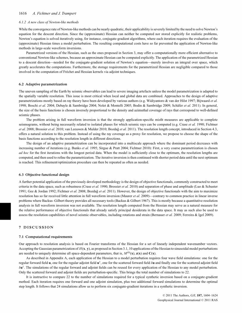
6.1.2 A new class of Newton-like methods

While the convergence rate of Newton-like methods can be nearly quadratic, their applicability is severely limited by the need to solve Newton’sequation for the descent direction. Since the (approximate) Hessian can neither be computed nor stored explicitly for realistic problems,Newton’s equation is solved iteratively using, for instance, conjugate-gradient algorithms, where each iteration requires the evaluation of the(approximate) Hessian times a model perturbation. The resulting computational costs have so far prevented the application of Newton-likemethods in large-scale waveform inversions.

Parametrized versions of the Hessian, such as the ones proposed in Section 3, may offer a computationally more efficient alternative toconventional Newton-like schemes, because an approximate Hessian can be computed explicitly. The application of the parametrized Hessianto a descent direction—needed for the conjugate-gradient solution of Newton’s equation—merely involves an integral over space, whichgreatly accelerates the computations. Furthermore, the storage requirements for the parametrized Hessian are negligible compared to thoseinvolved in the computation of Frechet and Hessian kernels via adjoint techniques.

6.2 Adaptive parametrization

The uneven sampling of the Earth by seismic observables can lead to severe imaging artefacts unless the model parametrization is adapted tothe spatially variable resolution. This issue is most critical when local and global data are combined. Approaches to the design of adaptiveparametrizations mostly based on ray theory have been developed by various authors (e.g. Widiyantoro & van der Hilst 1997; Bijwaard et al.1998; Boschi et al. 2004; Debayle & Sambridge 2004; Nolet & Montelli 2005; Bodin & Sambridge 2009; Schafer et al. 2011). In general,the size of the basis functions is chosen inversely proportional to the density and azimuthal coverage of rays that correspond to well-definedseismic phases.

The problem arising in full waveform inversion is that the strongly application-specific misfit measures are applicable to completeseismograms, without being necessarily related to isolated phases for which seismic rays can be computed (e.g. Crase et al. 1990; Fichtneret al. 2008; Brossier et al. 2010; van Leeuwen & Mulder 2010; Bozdag et al. 2011). The resolution length concept, introduced in Section 4.3,offers a natural solution to this problem. Instead of using the ray coverage as a proxy for resolution, we propose to choose the shape of thebasis functions according to the resolution length in different directions.

The design of an adaptive parametrization can be incorporated into a multiscale approach where the dominant period decreases withincreasing number of iterations (e.g. Bunks et al. 1995; Sirgue & Pratt 2004; Fichtner 2010): First, a very coarse parametrization is chosenad hoc for the first iterations with the longest period data. When the model is sufficiently close to the optimum, the resolution lengths arecomputed, and then used to refine the parametrization. The iterative inversion is then continued with shorter period data until the next optimumis reached. This refinement/optimization procedure can then be repeated as often as needed.

6.3 Objective functional design

A further potential application of the previously developed methodology is the design of objective functionals, commonly constructed to meetcriteria in the data space, such as robustness (Crase et al. 1990; Brossier et al. 2010) and separation of phase and amplitude (Luo & Schuster1991; Gee & Jordan 1992; Fichtner et al. 2008; Bozdag et al. 2011). However, the design of objective functionals with the aim to maximizeresolution has so far received little attention in full waveform inversion (Maurer et al. 2009)—contrary to common practice in linear inverseproblems where Backus–Gilbert theory provides all necessary tools (Backus & Gilbert 1967). This is mostly because a quantitative resolutionanalysis in full waveform inversion was not available. The resolution length computed from the Hessian may serve as a natural measure forthe relative performance of objective functionals that already satisfy principal desiderata in the data space. It may as such also be used toassess the resolution capabilities of novel seismic observables, including rotations and strain (Bernauer et al. 2009; Ferreira & Igel 2009).

7 D I S C U S S I O N

7.1 Computational requirements

Our approach to resolution analysis is based on Fourier transforms of the Hessian for a set of linearly independent wavenumber vectors.Accepting the Gaussian parametrization of H (x, y), as proposed in Section 3.1, 10 applications of the Hessian to sinusoidal model perturbationsare needed to uniquely determine all space-dependent parameters, that is, M (0)(x), z(x) and C(x).

As described in Appendix A, each application of the Hessian to a model perturbation requires four wave field simulations: one for theregular forward field u, one for the regular adjoint field u†, one for the scattered forward field δu and finally one for the scattered adjoint fieldδu†. The simulations of the regular forward and adjoint fields can be reused for every application of the Hessian to any model perturbation.Only the scattered forward and adjoint fields are perturbation-specific. This brings the total number of simulations to 22.

It is instructive to compare 22 to the number of simulations required for a typical synthetic inversion based on a conjugate-gradientmethod. Each iteration requires one forward and one adjoint simulation, plus two additional forward simulations to determine the optimalstep length. It follows that 24 simulations allow us to perform six conjugate-gradient iterations in a synthetic inversion.

C© 2011 The Authors, GJI, 187, 1604–1624



In realistic applications, however, the number of iterations is on the order of 20 (e.g. Tape et al. 2010; Fichtner et al. 2010), meaning thata synthetic inversion with only six iterations would be of little use. We therefore conclude that our approach is computationally more efficientthan synthetic inversions, while providing a much more complete characterization of resolution.

7.2 Gram–Charlier expansions

A weak point in our development lies in the parametrization of the Hessian by a Gram–Charlier series—truncated, in the simplest case, afterthe first-order term. As shown in Appendix B, Gram–Charlier series can be considered a variant of Taylor series. It follows that these twoexpansions potentially share some of their disadvantageous properties: slow convergence or even divergence, depending on the function thatwe wish to expand.

The efficiency of Gram–Charlier series generally depends on the choice of the parent function. This choice was straightforward in thecase of the ββ-component of the Hessian, Hββ , which is always roughly bell-shaped, that is, well-approximated by a Gaussian (see Fig. 2a).However, the off-diagonal elements Hβα and Hρα , shown in Figs 2(b) and 2(c), are less predictable. This makes the choice of a suitable andgeneric parent function difficult or even impossible. As a result of this complication, we did not attempt to parametrize Hβα and Hρα , meaningthat we are currently not able to study interparameter trade-offs in a comprehensive way. Clearly, a more powerful parametrization of theHessian would be a substantial improvement to our method.

7.3 Relation to migration deconvolution

Full waveform inversion can be regarded similar to various forms of migration (e.g. Tarantola 1984; Chavent & Plessix 1999; Nemeth et al.1999). Reverse-time migration, in particular, can be interpreted as the first iteration of a full waveform inversion, provided that measurementsare made only on body waves with an Ln norm misfit. A close link therefore exists between our approach and migration deconvolution used inexploration. Schuster & Hu (2000) computed migration PSFs for homogeneous media analytically. In the case of heterogeneous media, bothray theory (Hu et al. 2001) and spatially variable matched filters (Aoki & Schuster 2009) have been proposed to approximate PSFs. Thesewere then used for migration deconvolution or ‘deblurring’ (Hu et al. 2001; Aoki & Schuster 2009), much similar to the pre-conditioning ofa descent direction with the inverse approximate Hessian.

While the use of ray theory is restricted to well-defined and isolated high-frequency phases, the fitting of PSFs or their inverse with thehelp of matched filters could easily be generalized to full waveform inversion. In fact, our method proposed in Section 3 corresponds to amatched filter approach where one single input model is replaced by a set of input models that help to constrain the direction dependence ofPSFs.

Our method for resolution analysis is, however, more general than resolution analysis is migration, mostly because it is applicable on allscales, to all types of waves and to any misfit functional that one finds suitable for a particular application.

7.4 The problem of multiple minima

The weak point of our analysis is the assumption that the global minimum of χ has been found. In large-scale applications this assumptioncan hardly be verified, and there is no sufficiently efficient optimization algorithm that does not risk being trapped in a local minimum. Thisrestriction must be kept in mind when using the local Hessian in resolution analysis.

8 C O N C LU S I O N S

We have developed a new method for the quantitative resolution analysis in full seismic waveform inversion that overcomes the limitations ofchequer board type synthetic inversions while being computationally more efficient. Our approach is based on the quadratic approximationof the misfit functional and the parametrization of the Hessian operator in terms of parent functions and their successive derivatives. Thespace-dependent parameters can be computed efficiently using Fourier transforms of the Hessian for a small set of linearly independentwavenumber vectors.

In the simplest case where the Hessian is parametrized in terms of Gaussians, we can infer 3-D distributions of direction-dependentresolution length and the distortion introduced by the tomographic method. Our approach can be considered a generalization of the raydensity tensor (Kissling 1988) that quantifies the space-dependent azimuthal coverage, and therefore serves as a proxy for resolution in raytomography. The advantages of the parametrized Hessian compared to the ray density tensor include the applicability to any type of seismicwave, and the rigorous quantification of resolution, for instance, in terms of the resolution length. Furthermore, the parametrized Hessianmay be used for covariance and extremal bounds analysis, as proposed by Meju & Sakkas (2007) and Meju (2009).

A curious aspect of our approach is that information on the Hessian, and thus on resolution and trade-offs, can be obtained fromlinearized synthetic inversions where the initial model differs from the optimal model by a sinusoidal perturbation. This suggests thatsynthetics inversions are, at least in this sense, a useful tool, despite their well-known deficiencies (Leveque et al. 1993). Yet, they shouldnever be limited to single chequer board tests that bear little useful information.

C© 2011 The Authors, GJI, 187, 1604–1624



As a corollary to our developments, we propose several improvements to full waveform inversion techniques—all of which requirefurther investigations that are beyond the scope of this work. These include a new family of Newton-like methods, a pre-conditioner foroptimization schemes of the conjugate-gradient type, an approach to adaptive parametrization independent from ray theory and a strategy forobjective functional design that aims at maximizing resolution.

The most desirable improvement to our method would be more flexible but still rapidly converging parametrization of the Hessian. Thiswould allow us, for instance, to study trade-offs between model parameters of different physical nature.

While the examples given in Section 4 are very specific, the method itself is very general. It may, in particular, be adapted to smallerscale exploration scenarios and to wave-equation-based tomography techniques that employ, for instance, georadar (e.g Ernst et al. 2007;Meles et al. 2010) or microwave data (e.g. Chew & Lin 1995; Kosmas & Rappaport 2006).

A C K N OW L E D G M E N T S

We would like to thank our colleagues Moritz Bernauer, Christian Bohm, Cedric Legendre, Helle Pedersen and Florian Rickers for inspiringcomments and discussions. We are particularly grateful to Theo van Zessen for maintaining The STIG and GRIT, its little brother. Numerouscomputations were done on the Huygens IBM p6 supercomputer at SARA Amsterdam. Use of Huygens was sponsored by the NationalComputing Facilities Foundation (NCF) under the project SH-161-09 with financial support from the Netherlands Organisation for ScientificResearch (NWO). Furthermore, we would like to thank Gerard Schuster for making us aware of the relation between the Hessian and PSFs.The comments and thought-provoking questions of Yann Capdeville and an anonymous reviewer helped us to improve the text. Finally,Andreas Fichtner gratefully acknowledges Deutsche Bahn for all the endless delays that provided ample time to finish this manuscript.

R E F E R E N C E S

Aoki, N. & Schuster, G.T., 2009. Fast least-squares migration with a deblur-ring filter, Geophysics, 74, WCA83–WCA93.

Backus, G.E. & Gilbert, F., 1967. Numerical application of a formalism forgeophysical inverse problems, Geophys. J. R. astr. Soc., 13, 247–276.

Bamberger, A., Chavent, G. & Lailly, P., 1977. Une application de la theoriedu controle a un probleme inverse sismique, Ann. Geophys., 33, 183–200.

Bamberger, A., Chavent, G., Hemons, C. & Lailly, P., 1982. Inversion ofnormal incidence seismograms, Geophysics, 47, 757–770.

Bassin, C., Laske, G. & Masters, G., 2000. The current limits of resolu-tion for surface wave tomography in North America, EOS, Trans. Am.geophys. Un., 81, F897.

Bendinelli, O., Parmeggiani, G. & Zavatti, F., 1987. An analytical approxi-mation of the Hubble space telescope monochromatic point spread func-tion, J. Astrophys. Astron., 8, 343–350.

Bernauer, M., Fichtner, A. & Igel, H., 2009. Inferring earth structure fromcombined measurements of rotational and translational ground motions,Geophysics, 74, WCD41–WCD47.

Bijwaard, H., Spakman, W. & Engdahl, E.R., 1998. Closing the gap be-tween regional and global traveltime tomography, J. geophys. Res., 103,30 055–30 078.

Bleibinhaus, F., Hole, J.A. & Ryberg, T., 2007. Structure of the Cal-ifornia Coast Ranges and San Andreas Fault at SAFOD from seis-mic waveform inversion and reflection imaging, J. geophys. Res., 112,doi:10.1029/2006JB004611.

Bleibinhaus, F., Lester, R.W. & Hole, J.A., 2009. Applying waveform inver-sion to wide angle seismic surveys, Tectonophysics, 472, 238–248.

Bodin, T. & Sambridge, M., 2009. Seismic tomography with the reversiblejump algorithm, Geophys. J. Int., 178, 1411–1436.

Boschi, L., 2003. Measures of resolution in global body wave tomography,Geophys. Res. Lett., 30, doi:10.1029/2003GL018222.

Boschi, L., Ekstrom, G. & Kustowski, B., 2004. Multiple resolution sur-face wave tomography: the Mediterranean basin, Geophys. J. Int., 157,293–304.

Bozdag, E., Trampert, J. & Tromp, J., 2011. Misfit functions for full wave-form inversion based on instantaneous phase and envelope measurements,Geophys. J. Int., 185, 845–870.

Brossier, R., Operto, S. & Virieux, J., 2009. Seismic imaging of complex on-shore structures by 2D elastic frequency-domain full-waveform inversion,Geophysics, 74, WCC105–WCC118.

Brossier, R., Operto, S. & Virieux, J., 2010. Which data residual norm forrobust elastic frequency-domain full waveform inversion? Geophysics,75, R37–R46.

Bunks, C., Saleck, F.M., Zaleski, S. & Chavent, G., 1995. Multiscale seismicwaveform inversion, Geophysics, 60, 1457–1473.

Cara, M., Leveque, J.J. & Maupin, V., 1984. Density-versus-depth modelsfrom multimode surface waves, Geophys. Res. Lett., 11, 633–636.

Charlier, C.V.L., 1905. Uber die Darstellung willkurlicher Funktionen, Arkivfor Matematik, Astronomi och Fysik, 20(2), 1–35.

Chavent, G. & Plessix, R.-E., 1999. An optimal true-amplitude least-squaresprestack depth-migration operator, Geophysics, 64, 508–515.

Chen, P., 2011. Full-wave seismic data assimilation: theoretical back-ground and recent advances, Pure Appl. Geophys. 168, 1527–1552,doi:10.1007/s00024-010-0240-8.

Chen, P., Zhao, L. & Jordan, T.H., 2007. Full 3D tomography for thecrustal structure of the los angeles region, Bull. seism. Soc. Am., 97,1094–1120.

Chew, W.C. & Lin, J.H., 1995. A frequency-hopping approach for microwaveimaging of large inhomogeneous bodies, IEEE Microw. Guid. Wave Lett.,5, 439–441.

Cramer, H., 1957. Mathematical Methods of Statistics, Princeton UniversityPress, Princeton, NJ.

Crase, E., Pica, A., Noble, M., McDonald, J. & Tarantola, A., 1990. Robustelastic nonlinear waveform inversion: application to real data, Geophysics,55, 527–538.

Debayle, E. & Sambridge, M., 2004. Inversion of massive surface wave datasets: model construction and resolution assessment, J. geophys. Res., 109,B02316, doi:10.1029/2003JB002652.

Del Brio, E.B., Niguez, T.M. & Perote, J., 2009. Gram-Charlier densities: amultivariate approach, Quant. Finance, 9, 855–868.

Devaney, A.J., 1984. Geophysical diffraction tomography, IEEE Trans.Geos. Remote Sens., 22, 3–13.

Devilee, R.J.R., Curtis, A. & Roy-Chowdhury, K., 1999. An efficient, prob-abilistic neural network approach to solving inverse problems: invertingsurface wave velocities for Eurasian crustal thickness, J. geophys. Res.,104, 28 841–28 857.

Dondi, F., Betti, A., Blo, G. & Bighi, C., 1981. Statistical analysis of gas-chromatographic peaks by the Gram-Charlier series of type A and theEdgeworth-Cramer series, Anal. Chem., 53, 496–504.

Dziewonski, A.M. & Anderson, D.L., 1981. Preliminary reference Earthmodel, Phys. Earth planet. Inter., 25, 297–356.

Epanomeritakis, I., Akcelik, V., Ghattas, O. & Bielak, J., 2008. A Newton-CGmethod for large-scale three-dimensional elastic full waveform seismicinversion, Inverse Probl., 24, doi:10.1088/0266-5611/24/3/034015.

Ernst, J.R., Green, A.G., Maurer, H. & Holliger, K., 2007. Application of anew 2D time-domain full-waveform inversion scheme to crosshole radardata, Geophysics, 72, J53–J64.

C© 2011 The Authors, GJI, 187, 1604–1624



Fang, Y., Cheney, M. & Roecker, S., 2010. Imaging from sparse measure-ments, Geophys. J. Int., 180, 1289–1302.

Ferreira, A.M.G. & Igel, H., 2009. Rotational motions of seismic sur-face waves in a laterally heterogeneous Earth, Bull. seism. Soc. Am.,99, 1429–1436.

Fichtner, A., 2010. Full Seismic Waveform Modelling and Inversion,Springer, Heidelberg.

Fichtner, A. & Igel, H., 2008. Efficient numerical surface wave propagationthrough the optimization of discrete crustal models: a technique basedon non-linear dispersion curve matching (DCM), Geophys. J. Int., 173,519–533.

Fichtner, A. & Trampert, J., 2011. Hessian kernels of seismic data func-tionals based upon adjoint techniques, Geophys. J. Int., 185, 775–798.

Fichtner, A., Bunge, H.-P. & Igel, H., 2006. The adjoint method in seismol-ogy: I. Theory, Phys. Earth planet. Inter., 157, 86–104.

Fichtner, A., Kennett, B.L.N., Igel, H. & Bunge, H.-P., 2008. Theoreticalbackground for continental- and global-scale full-waveform inversion inthe time-frequency domain, Geophys. J. Int., 175, 665–685.

Fichtner, A., Kennett, B.L.N., Igel, H. & Bunge, H.-P., 2009. Full seis-mic waveform tomography for upper-mantle structure in the Australasianregion using adjoint methods, Geophys. J. Int., 179, 1703–1725.

Fichtner, A., Kennett, B.L.N., Igel, H. & Bunge, H.-P., 2010. Full waveformtomography for radially anisotropic structure: new insights into presentand past states of the Australasian upper mantle, Earth planet. Sci. Lett.,290, 270–280.

Gauthier, O., Virieux, J. & Tarantola, A., 1986. Two-dimensional nonlin-ear inversion of seismic waveforms: numerical results, Geophysics, 51,1387–1403.

Gee, L.S. & Jordan, T.H., 1992. Generalized seismological data functionals,Geophys. J. Int., 111, 363–390.

Gram, J.P., 1883. Ueber die Entwickelung reeller Functionen in Reihenmittelst der Methode der kleinsten Quadrate, Journal fur die reine undangewandte Mathematik, 94, 6–73.

Hingee, M., Tkalcic, H., Fichtner, A. & Sambridge, M., 2011. Seismic mo-ment tensor inversion using a 3-D structural model: applications for theAustralian region, Geophys. J. Int., 184, 949–964.

Hu, J., Schuster, G.T. & Valasek, P.A., 2001. Poststack migration deconvo-lution, Geophys. J. Int., 66, 939–952.

Igel, H., Djikpesse, H. & Tarantola, A., 1996. Waveform inversion of marinereflection seismograms for P impedance and Poisson’s ratio, Geophys. J.Int., 124, 363–371.

Jaynes, E.T., 2003. Probability Theory: The Logic of Science, CambridgeUniversity Press, Cambridge.

Kawai, K. & Geller, R.J., 2010. Waveform inversion for localised seismicstructure and an application to D′ ′ structure beneath the Pacific, J. geo-phys. Res., 115, doi:10.1029/2009JB006503.

Kissling, E., 1988. Geotomography with local earthquake data, Rev. Geo-phys., 26, 659–698.

Konishi, K., Kawai, K., Geller, R.J. & Fuji, N., 2009. MORB in the lower-most mantle beneath the western Pacific: evidence from waveform inver-sion, Earth planet. Sci. Lett., 278, 219–225.

Kosmas, P. & Rappaport, C.M., 2006. FDTD-based time reversal for mi-crowave breast cancer detection: localization in three dimensions, IEEETrans. Microw. Theo. Tech., 54, 1921–1927.

van Leeuwen, T. & Mulder, W.A., 2010. A correlation-based misfit cri-terion for wave-equation traveltime tomography, Geophys. J. Int., 182,1383–1394.

Leveque, J.J., Rivera, L. & Wittlinger, G., 1993. On the use of the checker-board test to assess the resolution of tomographic inversions, Geophys. J.Int., 115, 313–318.

Liu, D.C. & Nocedal, J., 1989. On the limited-memory BFGS method forlarge-scale optimisation, Math. Program., 45, 503–528.

Liu, Q. & Tromp, J., 2006. Finite-frequency kernels based on adjoint meth-ods, Bull. seismol. Soc. Am., 96, 2383–2397.

Luo, Y. & Schuster, G.T., 1991. Wave-equation traveltime inversion, Geo-physics, 56, 645–653.

Maurer, H., Greenhalgh, S. & Latzel, S., 2009. Frequency and spatial sam-

pling strategies for crosshole seismic waveform spectral inversion exper-iments, Geophysics, 74, WCC11–WCC21.

Meier, U., Curtis, A. & Trampert, J., 2007a. Fully nonlinear inversion offundamental mode surface waves for a global crustal model, Geophys.Res. Lett., 34, doi:10.1029/2007GL030989.

Meier, U., Curtis, A. & Trampert, J., 2007b. Global crustal thickness fromneural network inversion of surface wave data, Geophys. J. Int., 169,706–722.

Meju, M.A., 2009. Regularised extremal bounds analysis (REBA): an ap-proach to quantifying uncertainty in nonlinear geophysical inverse prob-lems, Geophys. Res. Lett., 36, doi:10:1029/2008GL036407.

Meju, M.A. & Sakkas, V., 2007. Heterogeneous crust and upper man-tle across southern Kenya and the relationship to surface deforma-tion as inferred from magnetotelluric imaging, J. geophys. Res., 112,doi:10:1029/2005JB004028.

Meles, G.A., van der Kruk, J., Greenhalgh, S.A., Ernst, J.R., Maurer, H. &Green, A.G., 2010. A new vector waveform inversion algorithm for simul-taneous updating of conductivity and permittivity parameters from com-bination of crosshole/borehole-to-surface GPR data, IEEE Trans. Geosc.Rem. Sens., 48, 3391–3407.

Mora, P., 1987. Nonlinear two-dimensional elastic inversion of multioffsetseismic data, Geophysics, 52, 1211–1228.

Mora, P., 1988. Elastic wave-field inversion of reflection and transmissiondata, Geophysics, 53, 750–759.

Mora, P., 1989. Inversion=migration+tomography, Geophysics, 54,1575–1586.

Nemeth, T., Wu, C. & Schuster, G.T., 1999. Least-squares migration ofincomplete reflection data, Geophysics, 64, 208–221.

Nolet, G. & Montelli, R., 2005. Optimal parametrization of tomographicmodels, Geophys. J. Int., 161, 365–372.

Nolet, G., Montelli, R. & Virieux, J., 1999. Explicit, approximate expres-sions for the resolution and a posteriori covariance of massive tomographicsystems, Geophys. J. Int., 138, 36–44.

Pankajakshan, P., Zhang, B., Blanc-Feraud, L., Kam, Z., Olivo-Marin, J.C. &Zerubia, J., 2000. Blind deconvolution for thin-layered confocal imaging,Appl. Opt., 48, 4437–4448.

Pavese, A., Artioli, G. & Prencipe, M., 1995. X-ray single-crystal diffrac-tion study of pyrope in the temperature range 30–973 k, Am. Mineral.,80, 457–464.

Peter, D., Boschi, L., Deschamps, F., Fry, B., Ekstrom, G. & Gi-ardini, D., 2008. A new finite-frequency shear-velocity model ofthe European-Mediterranean region, Geophys. Res. Lett., 35, doi:10.1029/2008GL034769.

Plessix, R.-E., 2006. A review of the adjoint-state method for computing thegradient of a functional with geophysical applications, Geophys. J. Int.,167, 495–503.

Pratt, R., Shin, C. & Hicks, G., 1998. Gauss-Newton and full Newton meth-ods in frequency domain seismic waveform inversion, Geophys. J. Int.,133, 341–362.

Ravaut, C., Operto, S., Importa, L., Virieux, J., Herrero, A. & dell’Aversana,P., 2004. Multi-scale imaging of complex structures from multi-fold wideaperture seismic data by frequency-domain full-wavefield inversions: ap-plication to a thrust belt, Geophys. J. Int., 159, 1032–1056.

Ritsema, J. & van Heijst, H., 2002. Constraints on the correlation of P- andS-wave velocity heterogeneity in the mantle from P, PP, PPP and PKPabtraveltimes, Geophys. J. Int., 149, 482–489.

Ritsema, J., vanHeijst, H. & Woodhouse, J.H., 1999. Complex shear wavevelocity structure imaged beneath Africa and Iceland, Science, 286,1925–1928.

Sambridge, M. & Mosegaard, K., 2002. Monte Carlo methods in geophysicalinverse problems, Rev. Geophys., 40, doi:10.1029/2000RG000089.

Samuelson, P.A., 1943. Fitting general Gram-Charlier series, Ann. Math.Stat., 14(2), 179–187.

Santosa, F. & Symes, W.W., 1988. Computation of the Hessian for least-squares solutions of inverse problems of reflection seismology, InverseProbl., 4, 211–233.

Sargan, J.D., 1975. Gram-Charlier approximations applied to t ratios ofk-class estimators, Econometrica, 43, 327–347.

C© 2011 The Authors, GJI, 187, 1604–1624



Sauer, P.W. & Heydt, G.T., 1979. Convenient multivariate Gram-Charliertype-A series, IEEE Trans. Comm., 27, 247–248.

Schafer, J., Boschi, L. & Kissling, E., 2011. Adaptively parametrized surfacewave tomography: methodology and a new model of the European uppermantle, Geophys. J. Int., 186, 1431–1453.

Schivardi, R. & Morelli, A., 2011. EPmantle: a 3-D transversely isotropicmodel of the upper mantle under the European Plate, Geophys. J. Int.,185, 469–484.

Schuster, G.T. & Hu, J., 2000. Green’s function for migration: continuousrecording geometry, Geophysics, 65, 167–175.

Sirgue, L. & Pratt, R.G., 2004. Efficient waveform inversion and imag-ing: a strategy for selecting temporal frequencies, Geophysics, 69, 231–248.

Smithyman, B., Pratt, R.G., Hayles, J. & Wittebolle, R., 2009. Detectingnear-surface objects with seismic waveform tomography, Geophysics, 74,WCC119–WCC127.

Spakman, W., 1991. Delay-time tomography of the upper mantle belowEurope, the Mediterranean and Asia Minor, Geophys. J. Int., 107, 309–332.

Takam Takougang, E.M. & Calvert, A., 2011. Application of waveformtomography to marine seismic reflection data from the Queen CharlotteBasin of western Canada, Geophysics, 76, B55–B70.

Takeuchi, H. & Saito, M., 1972. Seismic surface waves, in Methods in Com-putational Physics, Vol. 11, pp. 217–295, ed. Bolt B.A., Academic Press,New York, NY.

Tape, C., Liu, Q. & Tromp, J., 2007. Finite-frequency tomography usingadjoint methods: methodology and examples using membrane surfacewaves, Geophys. J. Int., 168, 1105–1129.

Tape, C., Liu, Q., Maggi, A. & Tromp, J., 2009. Adjoint tomography of thesouthern California crust, Science, 325, 988–992.

Tape, C., Liu, Q., Maggi, A. & Tromp, J., 2010. Seismic tomography ofthe southern California crust based upon spectral-element and adjointmethods, Geophys. J. Int., 180, 433–462.

Tarantola, A., 1984. Inversion of seismic reflection data in the acousticapproximation, Geophysics, 49, 1259–1266.

Tarantola, A., 1988. Theoretical background for the inversion of seismicwaveforms, including elasticity and attenuation, Pure appl. Geophys.,128, 365–399.

Tarantola, A., 2005. Inverse Problem Theory and Methods for Model Pa-rameter Estimation, 2nd edn., Society for Industrial and Applied Mathe-matics, Philadephia, PA.

Tromp, J., Tape, C. & Liu, Q., 2005. Seismic tomography, adjoint meth-ods, time reversal and banana-doughnut kernels, Geophys. J. Int., 160,195–216.

Trujillo, I., Aguerri, J.A.L. & Gutierrez, C.M., 2001. The effects of seeingon Sersic profiles, Mon. Not. R. astr. Soc., 321, 269–276.

Widiyantoro, S. & van der Hilst, R., 1997. Mantle structure beneath Indone-sia inferred from high-resolution tomographic imaging, Geophys. J. Int.,130, 167–182.

Wu, R.-S. & Toksoz, M.N., 1987. Diffraction tomography and multisourceholography applied to seismic imaging, Geophysics, 52, 11–25.

Yu, J.H., Wang, Y. & Schuster, G.T., 2002. Deconvolution of the psf of aseismic lens, in Image Reconstruction from Incomplete Data II, Proc.SPIE Vol. 4792, pp. 135–145, eds Bones, P.J., Fiddy, M.A. & Millane,R.P., SPIE, Bellingham, WA.

Zhang, B., Zerubia, J. & Olivo-Marin, J.C., 2007. Gaussian approximationof fluorescence microscope point-spread function models, Appl. Opt., 46,1819–1829.

Zielhuis, A. & Nolet, G., 1994. Shear-wave velocity variations in the uppermantle beneath central Europe, Geophys. J. Int., 117, 695–715.

A P P E N D I X A : H E S S I A N K E R N E L S

In this appendix, we provide a condensed recipe for the efficient computation of the Hessian applied to arbitrary model perturbations. In theinterest of notational compactness, we introduce the notion of Hessian kernels h(δm; x), defined as the Hessian H(x, y) applied to a modelperturbation δm(x).

h(δm; x) =∫

GH(x, y) δm(y) d3y . (A1)

More details including numerous examples may be found in Fichtner & Trampert (2011).

A1 The computation of Hessian kernels using adjoint techniques

As a preparatory step, we express the Frechet derivative of the misfit functional, ∇mχ δm, in terms of the Frechet kernel K(x)

∇mχ δm =∫

Gδm(x)T K(x) d3x . (A2)

In the exemplary case of an isotropic medium parametrized in terms of the S velocity β, the P velocity α and density ρ, the Frechet kernelhas three components, K = (Kβ, Kα, Kρ)T , and eq. (A2) can be expanded to

∇mχ δm =∫

GKβ (x) δβ(x) d3x +

∫G

Kα(x) δα(x) d3x +∫

GKρ(x) δρ(x) d3x . (A3)

The Frechet kernel can be computed efficiently with the help of adjoint techniques (e.g. Tarantola 1988; Tromp et al. 2005; Fichtner et al.2006; Liu & Tromp 2006; Plessix 2006; Chen 2011) that express K in terms of the current earth model m(x), the forward wave field u(x, t)and the adjoint wave field u†(x, t), that is,

K(x) = K(m, u, u†; x) . (A4)

The semicolon in eq. (A4) indicates that the variables to its left are fixed for a given realization of the space-dependent kernel K. We willadhere to this semicolon convention throughout the following developments. The adjoint wave field u†(x, t) is the solution of the adjoint waveequation, symbolically written in terms of the adjoint L† of the wave equation operator L

L†(m, u†) = f†(m) . (A5)

The adjoint source f† acts at the receiver positions, and its time evolution is completely determined by the misfit χ . This explains thedependence of f† on the earth model m. Note that both the forward and the adjoint wave fields, u and u†, are also dependent on m, that is,u = u(m; x) and u† = u†(m; x)

C© 2011 The Authors, GJI, 187, 1604–1624



To obtain a relation between the Frechet kernel K, the Hessian kernel h and the Hessian operator H, we differentiate eq. (A2) once morewith respect to m:

∇m∇mχ δm δm =∫

Gδm(x)T [∇mK(x) δm] d3x =

∫G

∫G

δm(x)T H(x, y) δm(y) d3x d3y . (A6)

It follows from (A6) that the Hessian kernel h from eq. (A2) is equal to the total Frechet derivative of the Frechet kernel K in thedirection of δm

h(δm; x) = ∇mK(x) δm . (A7)

To compute h explicitly, we exploit the dependence of the Frechet kernel on m, u and u†. The application of the chain rule to eq. (A7) thenyields

h(δm; x) = ∇mK(x) δm = ∂mK(m, u, u†; x) δm + K(m, δmu, u†; x) + K(m, u, δmu†; x) , (A8)

where ∂mK δm denotes the partial Frechet derivative of K in the direction δm; as opposed to the total Frechet derivative ∇mK δm. The symbolsδmu = ∇mu δm and δmu† = ∇mu†δm are the Frechet derivatives of the forward and adjoint fields, respectively.

Eq. (A8) reveals that the Hessian kernel h(δm; x) has three contributions. The first one of these, ∂mK(m, u, u†; x) δm, is localized at theperturbation δm, and has no obvious physical interpretation. The second contribution, K(m, δmu, u†; x), closely resembles the Frechet kernelfrom eq. (A4). However, instead of u it involves the derivative δmu, that can be interpreted as the scattered forward field that is excited whenu impinges upon the perturbation δm. In practice, δmu can be computed most conveniently using finite-differences such as

δmu ≈ 1

ν[u(m + ν δm) − u(m)] , (A9)

where ν must be sufficiently small to ensure the validity of the first-order approximation. From a physical point of view, this second contributionto the Hessian kernel describes the effect of second-order scattering from an arbitrary perturbation δm′ to δm and from there to the receiver.

The third contribution to the Hessian kernel, K(m, u, δmu†; x), also resembles the Frechet kernel (A4), but instead of the adjoint fieldu†, it involves the derivative δmu†. While δmu† may again be approximated with finite differences, for example,

δmu† ≈ 1

ν[u†(m + ν δm) − u†(m)] , (A10)

its computation and interpretation are more complex than it may seem. In fact, a model perturbation from m to m + δm has two effects: (1)the adjoint field u† is scattered when it impinges upon δm and (2) the adjoint source f† changes as well because a model perturbation affectsthe misfit χ that determines f†. It follows that the computation of u†(m + ν δm) requires the solution of the adjoint wave equation for theperturbed earth model and the perturbed adjoint source, that is,

L†(m + ν δm, u†) = f†(m + ν δm) . (A11)

In contrast to the second contribution K(m, δmu, u†; x), the third contribution K(m, u, δmu†; x) accounts for both the first-order scatteringthat leads to the perturbation of the adjoint source and the second-order scattering between δm and the receiver.

A2 A realistic example

To attach physical intuition to the above equations, we consider an isotropic medium parametrized in terms of the P velocity α, the S velocityβ and density ρ, that is, m = (α, β, ρ)T . The Frechet kernel Kβ is given by (e.g. Tromp et al. 2005; Liu & Tromp 2006; Fichtner 2010)

Kβ = 4ρβ

∫εi j ε

†i j dt − 4ρα

∫εi i ε

†j j dt , (A12)

where ε† = 12 [∇u† + (∇u†)T ] is the strain tensor computed from the adjoint field. For the specific case of a 25 s Love wave recorded at 25.2◦

epicentral distance, the Frechet kernel for a cross-correlation time shift measurement (Luo & Schuster 1991) occupies a cigar-shaped volumethat extends from the source to the receiver (Fig. A1).

Making use of eq. (A8) we find that the β-component of the Hessian kernel corresponding to an S velocity perturbation δm = (0, δβ, 0)T ,that is, hβ (δβ) = ∫

Hββ δβ d3y, is given by

hβ (δβ) = 4ρ δβ

∫εi j ε

†i j dt︸︷︷︸

∂m K(m,u,u†) δm

+ 4ρβ

∫δβεi j εi j dt − 4ρα

∫δβεi i ε

†j j dt︸︷︷︸

K(m,δm u,u†)

+ 4ρβ

∫εi j δβε

†i j dt − 4ρα

∫εi i δβε

†j j dt︸︷︷︸

K(m,u,δm u†)

. (A13)

The contribution ∂mK(m, u, u†) δm can be computed directly from the Frechet kernels. Additional simulations are needed for K(m, δmu, u†)and K(m, u, δmu†) because these involve the differentiated forward and adjoint fields, δu and δu†, that can be computed most convenientlywith the help of the finite-difference approximations (A9) and (A10).

The three contributions to the Hessian kernel hβ (δβ) for a point perturbation δβ located beneath southern Sardinia are shown separatelyin the top row of Fig. A2. The contribution K(m, u, δmu†) is a superposition of two components, labelled F and S. These correspond to theprimary influence zone represented by the approximate Hessian (F) and to the secondary influence zone where second-order scattering affectsthe measurement. The contribution K(m, δmu, u†) only extends from the receiver to δβ. Second-order scattering from δβ to an S velocity

C© 2011 The Authors, GJI, 187, 1604–1624



Figure A1. (Left) N–S-component synthetic seismogram computed using a spectral-element method (Fichtner & Igel 2008). The time window around theLove wave used to compute Frechet and Hessian kernels is shaded in grey. The dominant period is 25 s. (Right) Frechet kernel KvS for a cross-correlationtime shift measurement on the N–S-component Love wave shown to the left. The source and receiver positions are marked by + and •, respectively. Figuremodified from Fichtner & Trampert (2011).

Figure A2. Hessian kernels plotted at the surface of the Earth. The position of the S velocity perturbation δβ is indicated by ◦. Top row: The individualcontributions K(m, u, δmu†), ∂mK(m, u, u†) δm and K(m, δmu, u†) (from left to right). The contribution K(m, u, δmu†) has two components, labelled F andS. These represent a primary influence zone corresponding to the approximate Hessian (F), and to a secondary influence zone where second-order scatteringaffects the measurement (S). Bottom row: The complete Hessian kernel hβ (δβ). The contribution from second-order scattering is again encircled by a dottedcurve and labelled S. Figure modified from Fichtner & Trampert (2011).

perturbation within the non-zero parts of K(m, δmu, u†) has an effect on the measurement. Finally, ∂mK(m, u, u†) δm is restricted to thevolume occupied by δβ. The complete Hessian kernel hβ (δβ) is shown in the bottom row of Fig. A2. It can be interpreted as the continuousrepresentation of the row of the Hessian matrix that corresponds to the basis function coincident with δβ. The fully discrete row is obtainedby projecting hβ (δβ) onto the basis functions. For a more detailed discussion of Hessian kernels, the reader is referred to Fichtner & Trampert(2011).

A P P E N D I X B : M U LT I VA R I AT E G R A M – C H A R L I E R S E R I E S

The resolution analysis proposed in Section 3 rests on the approximation of the Hessian H(x, y) by a linear sum of terms that consist ofa parent function and its successive derivatives. Approximation problems of this type have been studied at least since the end of the 19thcentury (e.g. Gram 1883; Charlier 1905; Samuelson 1943), and the special case where the parent function is a Gaussian became known theGram–Charlier series. While originally introduced in a purely mathematical context, Gram–Charlier series became a popular tool for theapproximation of 1-D densities in a variety of fields including econometrics (e.g. Sargan 1975), analytical chemistry (e.g. Dondi et al. 1981)and mineral physics (e.g. Pavese et al. 1995). Generalizations to higher dimensions and applications in a geophysical context have, however,remained an exception (e.g. Sauer & Heydt 1979; Gee & Jordan 1992; Del Brio et al. 2009). In the following paragraphs, we describeGram–Charlier approximations in N ≥ 1 dimensions that are based on the representation of a function in terms of its cumulants.

B1 Moments and cumulants

We consider the spatial Fourier transform of a function f (x), defined as

f (k) =∫

RNf (x) eikT x dN x . (B1)

C© 2011 The Authors, GJI, 187, 1604–1624



Expanding f (x) into a Taylor series, yields

f (k) = M (0) + ikT M(1) + i2

2!kT M(2)k + · · · , (B2)

where the components of the tensorial Taylor coefficients M(n) are given by

M (n)i jk... = 1

i n

(∂

∂xi

∂

∂x j

∂

∂xk. . .

)f |k=0 . (B3)

Introducing (B1) into (B3), reveals that the coefficients M (n)ijk... are equal to the moments of f .

M (n)i jk... =

∫RN

(xi x j xk . . .) f (x) dN x . (B4)

Similar to (B2), the cumulants F(n) of f are defined through the Taylor coefficients of log f .

log f (k) = F (0) + ikT F(1) + i2

2!kT F(2)k + · · · . (B5)

Upon using

F (n)i jk... = 1

i n

(∂

∂xi

∂

∂x j

∂

∂xk. . .

)log f |k=0 , (B6)

we find that the first three cumulants and moments are related as follows:

F (0) = log M (0) , F (1)i = M (1)

i

M (0), F (2)

i j = 1

M (0)

(M (2)

i j − M (1)i M (1)

j

M (0)

). (B7)

By definition (eq. B5), the cumulants are additive under convolution.

B2 Wavenumber-domain Gram–Charlier series

Our goal is to approximate f in terms of a suitably chosen parent function g. With the help of eq. (B5), we can express the spectrum f as

f (k) = f (k)

g(k)g(k) = exp

[(F (0) − G(0)

) + ikT(F(1) − G(1)

) + i2

2!kT

(F(2) − G(2)

)k + · · ·

]g(k) , (B8)

where F(n) and G(n) are the cumulants of f and g, respectively. Eq. (B8) provides a very general expression of f , that can be greatly simplifiedthrough the judicious choice of g. Thus, in the context of resolution analysis, the parent function should already capture the principalcharacteristics of the PSF. We obtain the wavenumber-domain representation of the classical Gram–Charlier A series when the parent functiong is equal to the normalized Gaussian

g(x) =√

det C

(2π )N/2exp

[−1

2(x − z)T C (x − z)

](B9)

with the cumulants

G(0) = 0 , G(1) = z , G(2) = C−1 , G(n>2) = 0 . (B10)

This eliminates the cumulants of g with orders greater than 2 from eq. (B8). Since we are still free to choose the specific values of G(1) andG(2), we let G(1) = F(1) and G(2) = F(2), so that eq. (B8) reduces to

f (k) = M (0) exp

[i3

3!F (3)

i jk ki k j kk + i4

4!F (4)

i jkl ki k j kkkl + · · ·]

exp

(ikT z − 1

2kT C−1k

), (B11)

where M (0) is the zeroth moment of f . Eq. (B11) expresses the spectrum of f in terms of its cumulants with orders n ≥ 3, and its first threemoments: the norm M (0), the expected value z and the covariance C. By expanding the first exponential on the left-hand side of (B11) into aTaylor series, we obtain the following approximation:

f (k) = M (0)

[1 + i3

3!F (3)

i jk ki k j kk + i4

4!F (4)

i jkl ki k j kkkl + · · ·]

exp

(−ikT z − 1

2kT C−1k

). (B12)

While the coefficients of orders 3, 4 and 5 are equal to F(3), F(4) and F(5), respectively, the higher order coefficients involve products ofcumulants.

B3 Space-domain Gram–Charlier series

To translate the wavenumber-domain Gram-Charlier series (B11) into the space domain, we exploit the Fourier correspondence

exp(ik j

)f (k) ↔ exp

(− ∂

∂x j

)f (x) . (B13)

C© 2011 The Authors, GJI, 187, 1604–1624



Figure B1. (Left) Real part of the step function spectrum f (k) from eq. (B17), plotted in black. The Gram–Charlier approximations of orders 0, 3 and 7 areshown in different red tones. (Centre) The same as to the left, but for the imaginary part of f (k). (Right) The space-domain step function from (B17) and itsGram–Charlier approximations of orders 0, 3 and 7.

With the help of (B13), eq. (B11) transforms to

f (x) = M (0)

√det C

(2π )N/2exp

[(−1)3

3!F (3)

i jk

∂

∂xi

∂

∂x j

∂

∂xk+ (−1)4

4!F (4)

i jkl

∂

∂xi

∂

∂x j

∂

∂xk

∂

∂xl+ · · ·

]exp

[−1

2(x − z)T C (x − z)

]. (B14)

Again expanding the first exponential on the left-hand side of (B14), yields a more useful equation

f (x) = M (0)

√det C

(2π )N/2

[1 + (−1)3

3!F (3)

i jk

∂

∂xi

∂

∂x j

∂

∂xk+ (−1)4

4!F (4)

i jkl

∂

∂xi

∂

∂x j

∂

∂xk

∂

∂xl+ · · ·

]exp

[−1

2(x − z)T C (x − z)

]. (B15)

The Gram–Charlier series from (B15) can be interpreted as the summation of contributions with increasing wavelength. The truncatedexpansion

f (x) ≈ M (0)

√det C

(2π )N/2exp

[−1

2(x − z)T C (x − z)

](B16)

is, in this sense, a long-wavelength approximation.

B4 Properties of the Gram–Charlier expansion

To illustrate the nature of Gram-Charlier expansion, we consider the step function

f (x) =

⎧⎪⎪⎨⎪⎪⎩1 , −2 ≤ x < 0 ,

12 , 0 ≤ x ≤ 2 ,

0 , otherwise ,

f (k) = [2 exp(−ik) + exp(ik)] sinc(k) (B17)

as a simple 1-D example. The wavenumber- and space-domain Gram–Charlier expansions of orders 0, 3 and 7 are shown in Fig. B1. The0th-order approximation in the wavenumber domain is a Gaussian that closely matches the exact spectrum f (k) within the wavenumberrange ±1 m−1. The corresponding space-domain approximation is a Gaussian where the first three moments are equal to those of the stepfunction (B17). Higher order contributions account for the skewness of f (x), but the improvements are limited to the wavenumber interval[−π , π ], outside of which the Taylor series from eq. (B11) does not converge. It follows that the Gram–Charlier expansion of (B17) isalways a low-wavenumber approximation, even when infinitely many coefficients are included. This behaviour is typical in the sense that aGram–Charlier series does not necessarily converge, and if it does, the convergence may be slow (e.g. Samuelson 1943; Cramer 1957).

The essence of this example is that the Gram–Charlier series should be considered a tool to capture the gross features of a function witha few coefficients, where the meaning of gross feature is determined by the choice of the parent function.

C© 2011 The Authors, GJI, 187, 1604–1624


resolution analysis in full waveform inversionfichtner/papers/2011_resolution.pdf · resolution in...

Documents