full waveform inversion for high resolution seismic ... · pdf filefull waveform inversion for...
TRANSCRIPT
Full waveform inversion for high resolution seismic imaging: HPC issueson recent applications and ongoing research.
L. Metivier1,2, R. Brossier2, Q. Merigot3, A. Minuissi4,S. Operto4, E. Oudet1, J. Virieux2
1LJK, CNRS & Universite Grenoble Alpes2ISTerre, Universite Grenoble Alpes
3CEREMADE, CNRS & Universite Paris-Dauphine4Geoazur, CNRS & Universite Nice Sophia Antipolis
http://seiscope2.osug.fr
4iemes Journees Scientifiques Equip@Meso : Sciences de l’Univers, Toulouse,CALMIP, 26 et 27 Novembre 2015
SEISCOPE
L. Metivier et al. (Univ. Grenoble, CNRS) Full waveform inversion 27/11/2015 1 / 27
Outline
1 Introduction: principle of full waveform inversion
2 Example of application: 3D acoustic frequency-domain FWI
3 Reducing the sensitivity to the initial model accuracy using an optimal transport distance
L. Metivier et al. (Univ. Grenoble, CNRS) Full waveform inversion 27/11/2015 2 / 27
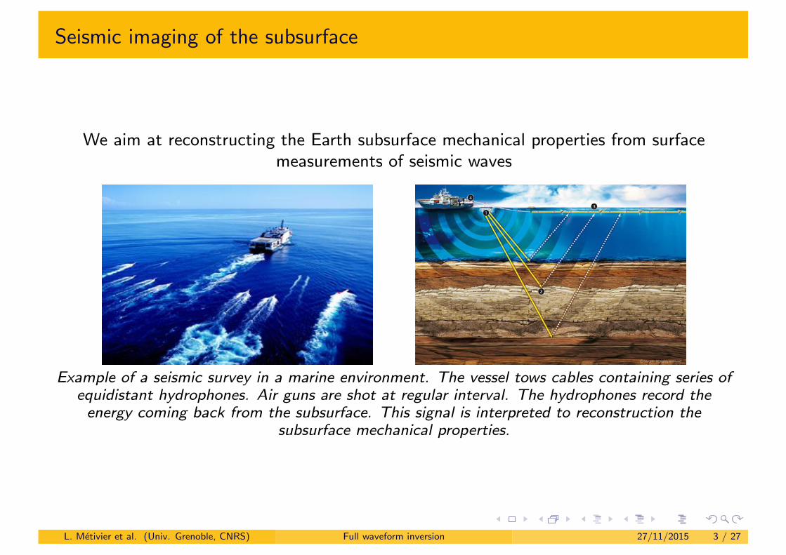
Seismic imaging of the subsurface
We aim at reconstructing the Earth subsurface mechanical properties from surfacemeasurements of seismic waves
Example of a seismic survey in a marine environment. The vessel tows cables containing series ofequidistant hydrophones. Air guns are shot at regular interval. The hydrophones record theenergy coming back from the subsurface. This signal is interpreted to reconstruction the
subsurface mechanical properties.
L. Metivier et al. (Univ. Grenoble, CNRS) Full waveform inversion 27/11/2015 3 / 27
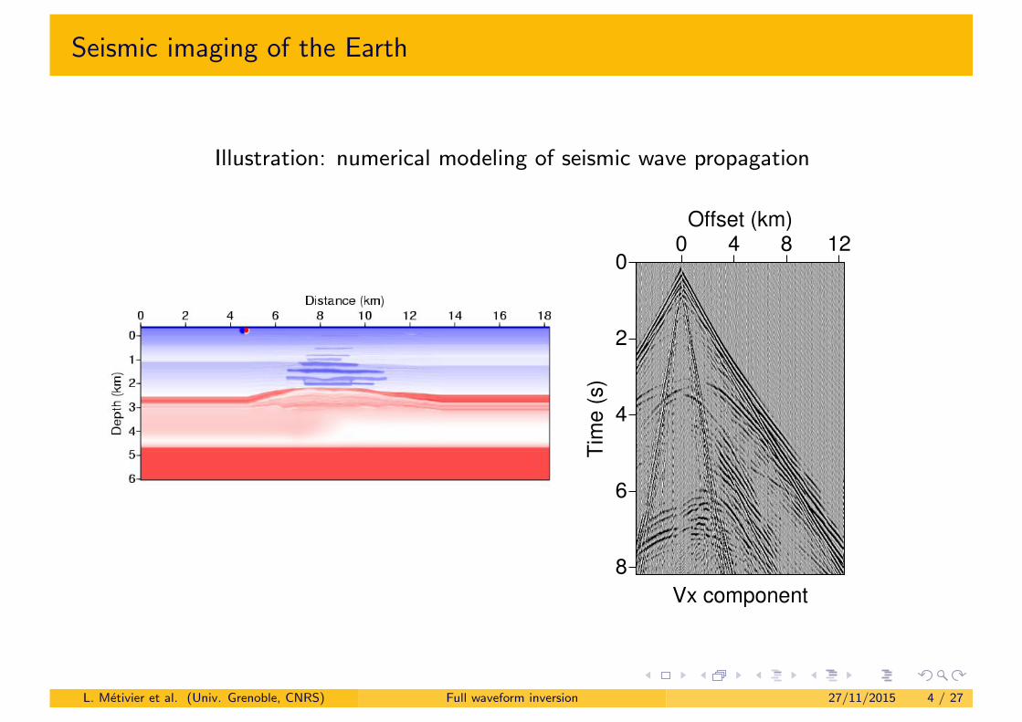
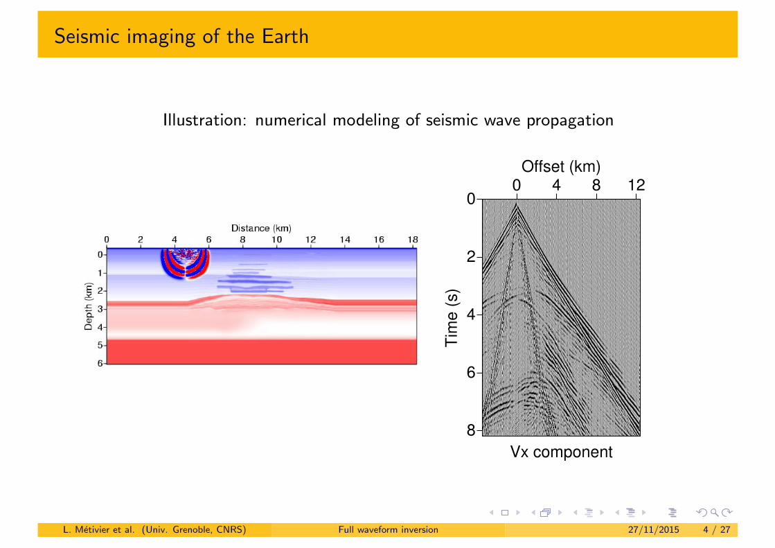
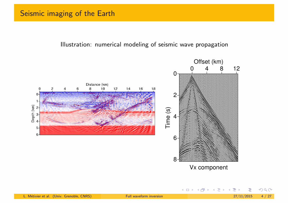
Seismic imaging of the Earth
Illustration: numerical modeling of seismic wave propagation
L. Metivier et al. (Univ. Grenoble, CNRS) Full waveform inversion 27/11/2015 4 / 27
Seismic imaging of the Earth
Illustration: numerical modeling of seismic wave propagation
L. Metivier et al. (Univ. Grenoble, CNRS) Full waveform inversion 27/11/2015 4 / 27
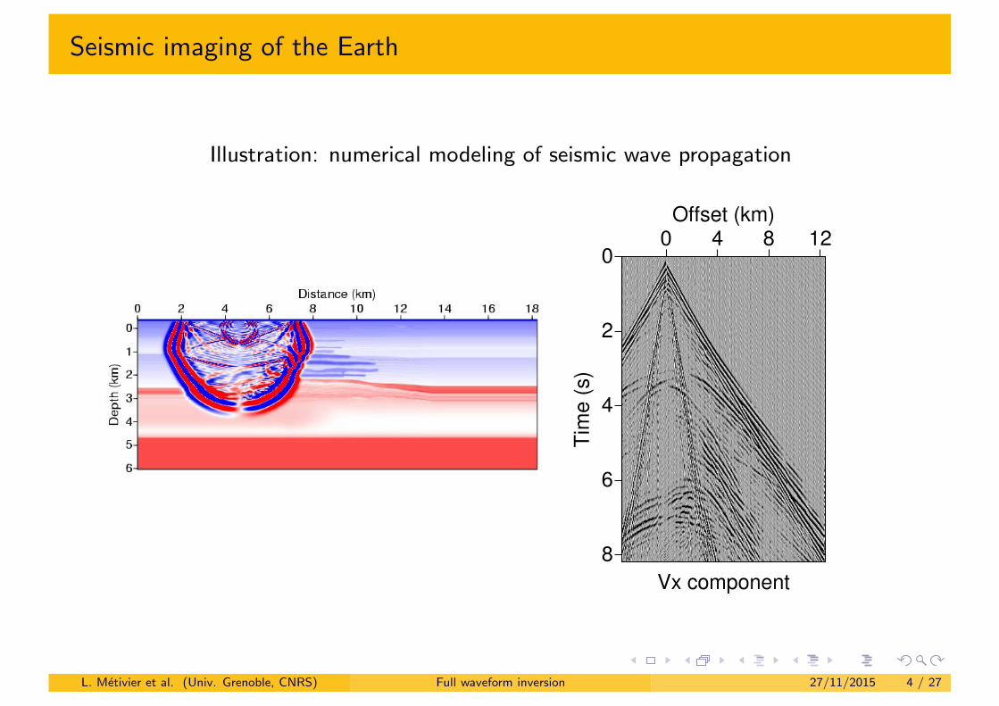
Seismic imaging of the Earth
Illustration: numerical modeling of seismic wave propagation
L. Metivier et al. (Univ. Grenoble, CNRS) Full waveform inversion 27/11/2015 4 / 27

Seismic imaging of the Earth
Illustration: numerical modeling of seismic wave propagation
L. Metivier et al. (Univ. Grenoble, CNRS) Full waveform inversion 27/11/2015 4 / 27
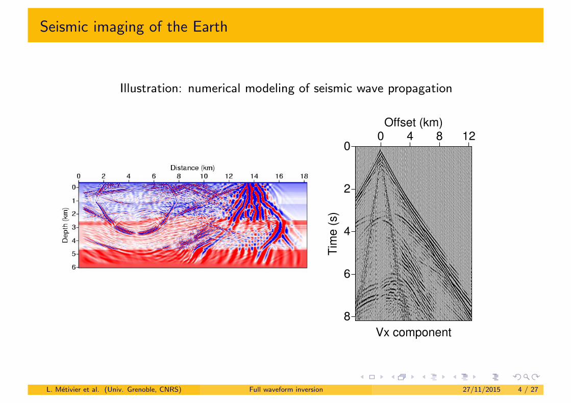
Seismic imaging of the Earth
Illustration: numerical modeling of seismic wave propagation
L. Metivier et al. (Univ. Grenoble, CNRS) Full waveform inversion 27/11/2015 4 / 27
Seismic imaging of the Earth
Illustration: numerical modeling of seismic wave propagation
L. Metivier et al. (Univ. Grenoble, CNRS) Full waveform inversion 27/11/2015 4 / 27
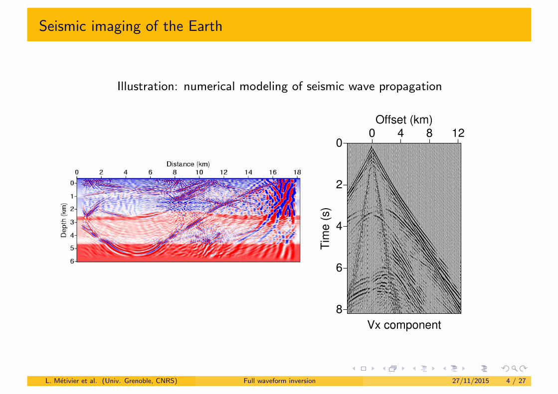
Seismic imaging of the Earth
Illustration: numerical modeling of seismic wave propagation
L. Metivier et al. (Univ. Grenoble, CNRS) Full waveform inversion 27/11/2015 4 / 27
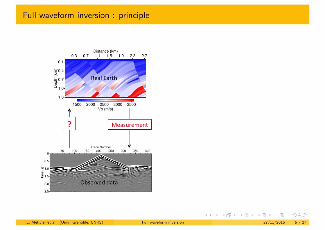
Full waveform inversion : principle
28th'September'2012'
Full(waveform(inversion((FWI)(F(Principle(
Progress'MeeMng'';''Isabella'MASONI' 7'
0.1
0.4
0.7
1.0
1.3
Depth
(km
)0.3 0.7 1.1 1.5 1.9 2.3 2.7
Distance (km)
1500 2000 2500 3000 3500Vp (m/s)
0
0.5
1.0
1.5
2.0
2.5
Tim
e (
s)
50 100 150 200 250 300 350 400Trace Number
Measurement'?(
Real'Earth'
Observed'data'
L. Metivier et al. (Univ. Grenoble, CNRS) Full waveform inversion 27/11/2015 5 / 27
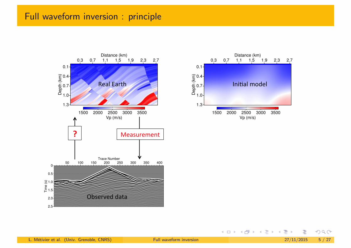
Full waveform inversion : principle
28th'September'2012'
Full(waveform(inversion((FWI)(F(Principle(
Progress'MeeMng'';''Isabella'MASONI' 8'
0.1
0.4
0.7
1.0
1.3
Depth
(km
)0.3 0.7 1.1 1.5 1.9 2.3 2.7
Distance (km)
1500 2000 2500 3000 3500Vp (m/s)
0.1
0.4
0.7
1.0
1.3
Depth
(km
)
0.3 0.7 1.1 1.5 1.9 2.3 2.7Distance (km)
1500 2000 2500 3000 3500Vp (m/s)
0
0.5
1.0
1.5
2.0
2.5
Tim
e (
s)
50 100 150 200 250 300 350 400Trace Number
Measurement'?(
IniMal'model'Real'Earth'
Observed'data'
L. Metivier et al. (Univ. Grenoble, CNRS) Full waveform inversion 27/11/2015 5 / 27
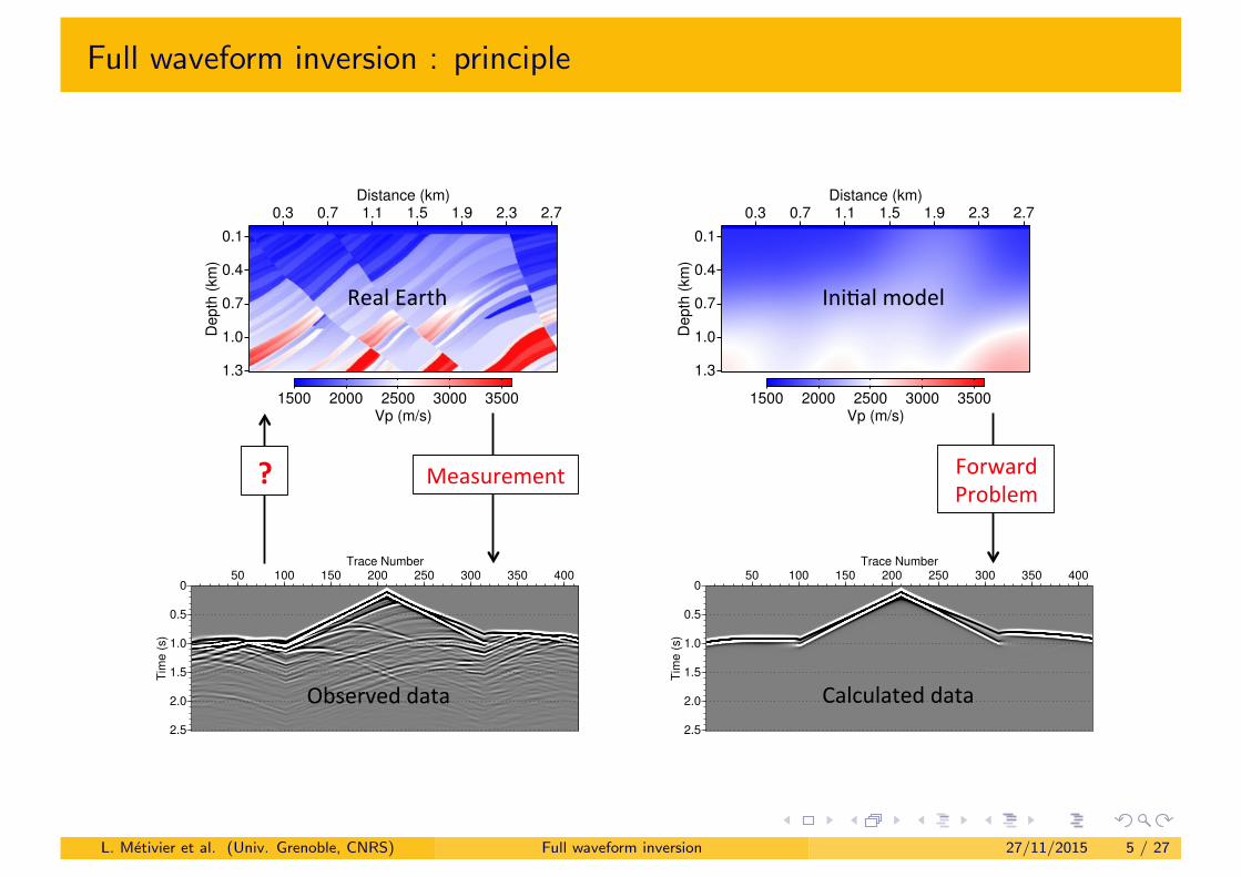
Full waveform inversion : principle
28th'September'2012'
Full(waveform(inversion((FWI)(F(Principle(
Progress'MeeMng'';''Isabella'MASONI' 9'
0.1
0.4
0.7
1.0
1.3
Depth
(km
)0.3 0.7 1.1 1.5 1.9 2.3 2.7
Distance (km)
1500 2000 2500 3000 3500Vp (m/s)
0.1
0.4
0.7
1.0
1.3
Depth
(km
)
0.3 0.7 1.1 1.5 1.9 2.3 2.7Distance (km)
1500 2000 2500 3000 3500Vp (m/s)
0
0.5
1.0
1.5
2.0
2.5
Tim
e (
s)
50 100 150 200 250 300 350 400Trace Number
0
0.5
1.0
1.5
2.0
2.5
Tim
e (
s)
50 100 150 200 250 300 350 400Trace Number
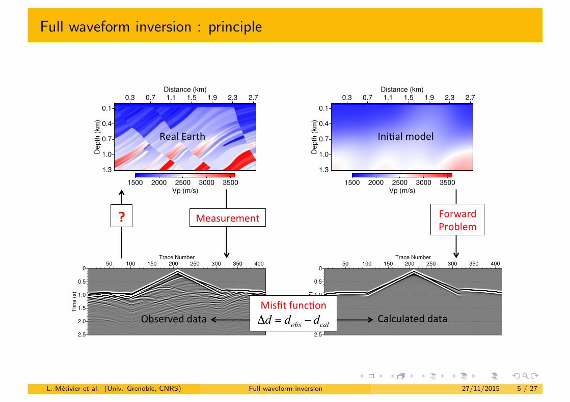
Measurement'?( Forward'Problem'
IniMal'model'Real'Earth'
Calculated'data'Observed'data'
L. Metivier et al. (Univ. Grenoble, CNRS) Full waveform inversion 27/11/2015 5 / 27
Full waveform inversion : principle
28th'September'2012'
Full(waveform(inversion((FWI)(F(Principle(
Progress'MeeMng'';''Isabella'MASONI' 10'
0.1
0.4
0.7
1.0
1.3
Depth
(km
)0.3 0.7 1.1 1.5 1.9 2.3 2.7
Distance (km)
1500 2000 2500 3000 3500Vp (m/s)
0.1
0.4
0.7
1.0
1.3
Depth
(km
)
0.3 0.7 1.1 1.5 1.9 2.3 2.7Distance (km)
1500 2000 2500 3000 3500Vp (m/s)
0
0.5
1.0
1.5
2.0
2.5
Tim
e (
s)
50 100 150 200 250 300 350 400Trace Number
0
0.5
1.0
1.5
2.0
2.5
Tim
e (
s)
50 100 150 200 250 300 350 400Trace Number
Measurement'?( Forward'Problem'
IniMal'model'Real'Earth'
Calculated'data'Observed'data'Misfit'funcMon'
'Δd = dobs − dcal
L. Metivier et al. (Univ. Grenoble, CNRS) Full waveform inversion 27/11/2015 5 / 27
Full waveform inversion : principle
28th'September'2012'
Full(waveform(inversion((FWI)(F(Principle(
Progress'MeeMng'';''Isabella'MASONI' 11'
0.1
0.4
0.7
1.0
1.3
Depth
(km
)0.3 0.7 1.1 1.5 1.9 2.3 2.7
Distance (km)
1500 2000 2500 3000 3500Vp (m/s)
0.1
0.4
0.7
1.0
1.3
Depth
(km
)
0.3 0.7 1.1 1.5 1.9 2.3 2.7Distance (km)
1500 2000 2500 3000 3500Vp (m/s)
0
0.5
1.0
1.5
2.0
2.5
Tim
e (
s)
50 100 150 200 250 300 350 400Trace Number
0
0.5
1.0
1.5
2.0
2.5
Tim
e (
s)
50 100 150 200 250 300 350 400Trace Number
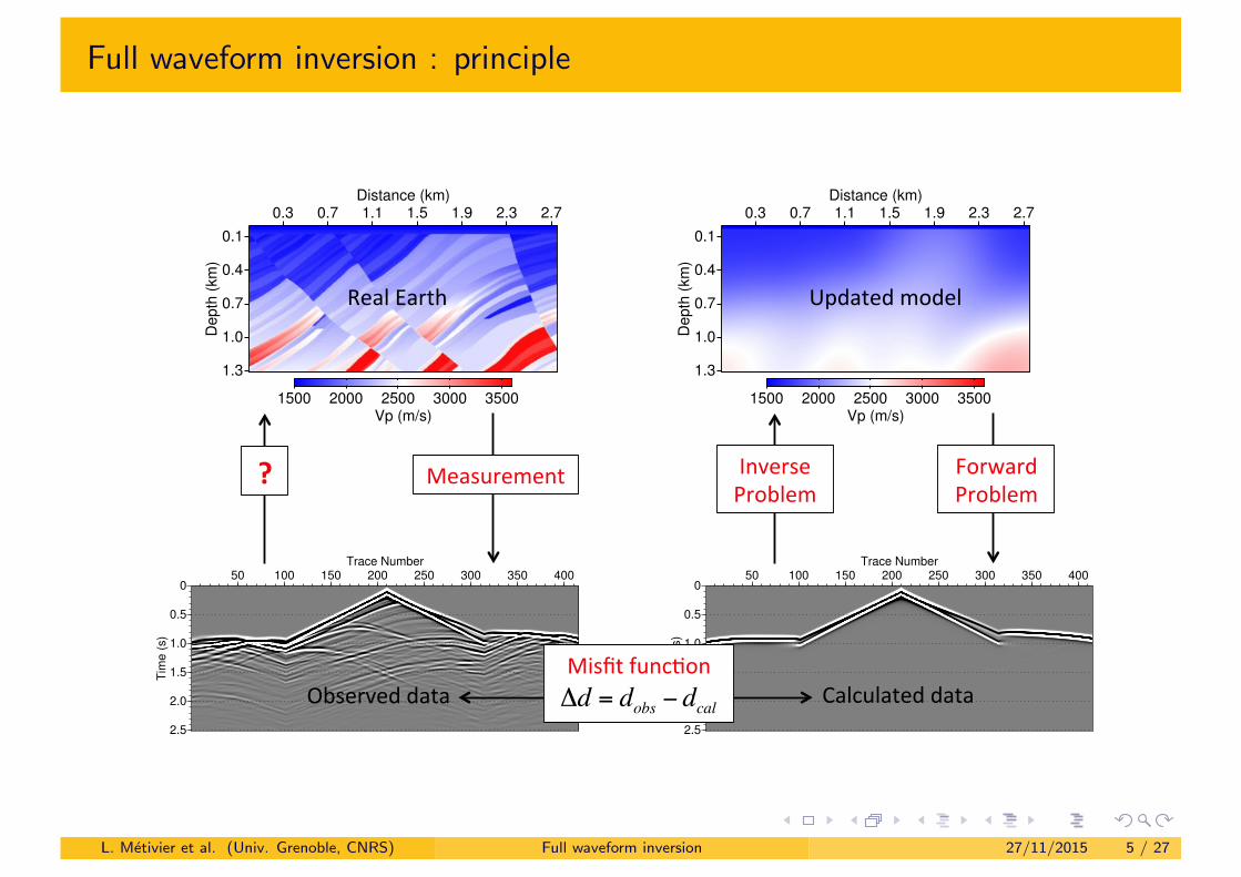
Measurement'?( Forward'Problem'
Inverse'Problem'
Updated'model'Real'Earth'
Calculated'data'Observed'data'Misfit'funcMon'
'Δd = dobs − dcal
L. Metivier et al. (Univ. Grenoble, CNRS) Full waveform inversion 27/11/2015 5 / 27
Full waveform inversion : principle
0
0.5
1.0
1.5
2.0
2.5
Tim
e (
s)
50 100 150 200 250 300 350 400Trace Number
0.1
0.4
0.7
1.0
1.3
Depth
(km
)
0.3 0.7 1.1 1.5 1.9 2.3 2.7Distance (km)
1500 2000 2500 3000 3500Vp (m/s)
28th'September'2012'
Full(waveform(inversion((FWI)(F(Principle(
Progress'MeeMng'';''Isabella'MASONI' 12'
0.1
0.4
0.7
1.0
1.3
Depth
(km
)0.3 0.7 1.1 1.5 1.9 2.3 2.7
Distance (km)
1500 2000 2500 3000 3500Vp (m/s)
0
0.5
1.0
1.5
2.0
2.5
Tim
e (
s)
50 100 150 200 250 300 350 400Trace Number
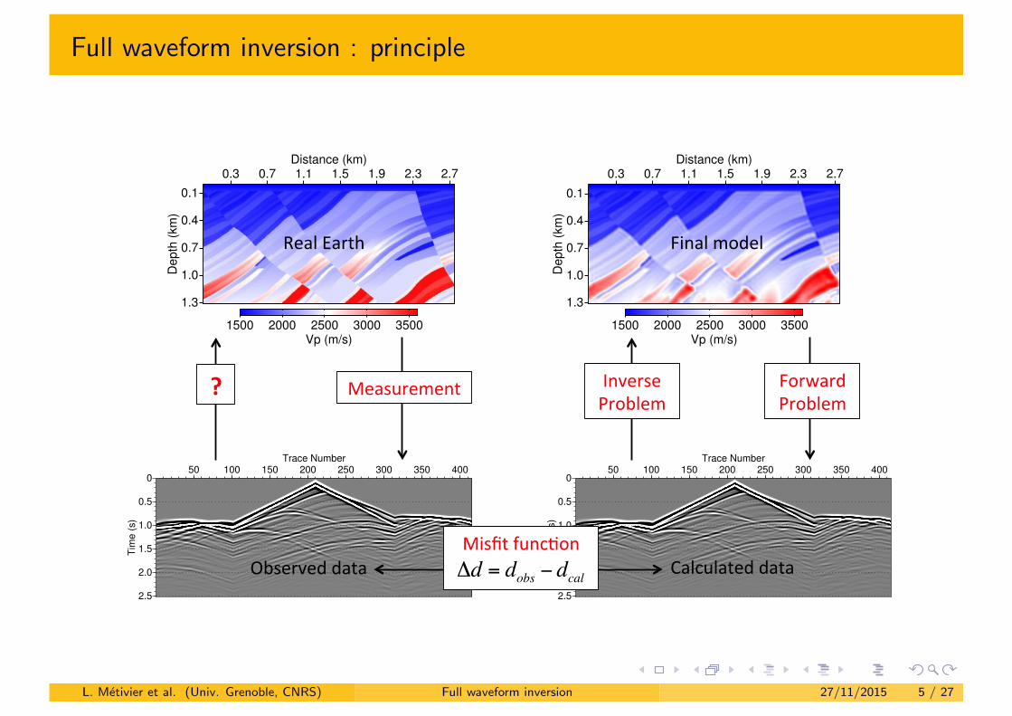
Measurement'?( Forward'Problem'
Inverse'Problem'
Final'model'Real'Earth'
Calculated'data'Observed'data'Misfit'funcMon'
'Δd = dobs − dcal
L. Metivier et al. (Univ. Grenoble, CNRS) Full waveform inversion 27/11/2015 5 / 27
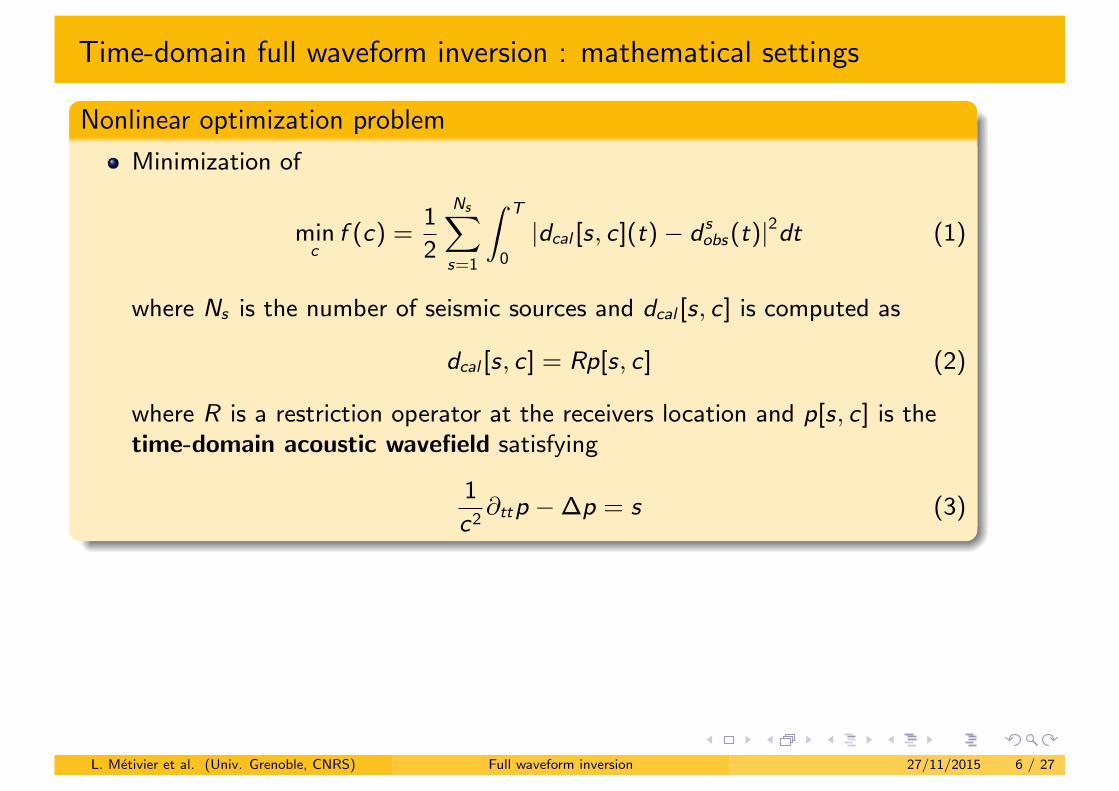
Time-domain full waveform inversion : mathematical settings
Nonlinear optimization problem
Minimization of
minc
f (c) =12
NsX
s=1
Z T
0
|dcal [s, c](t)� d sobs(t)|2dt (1)
where Ns is the number of seismic sources and dcal [s, c] is computed as
dcal [s, c] = Rp[s, c] (2)
where R is a restriction operator at the receivers location and p[s, c] is thetime-domain acoustic wavefield satisfying
1c2
@ttp ��p = s (3)
L. Metivier et al. (Univ. Grenoble, CNRS) Full waveform inversion 27/11/2015 6 / 27
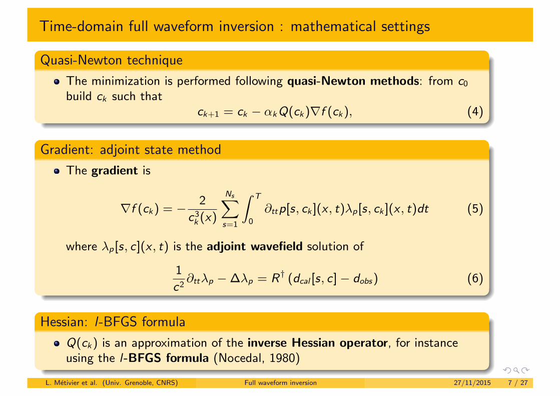
Time-domain full waveform inversion : mathematical settings
Quasi-Newton technique
The minimization is performed following quasi-Newton methods: from c0
build ck such thatck+1 = ck � ↵kQ(ck)rf (ck), (4)
Gradient: adjoint state method
The gradient is
rf (ck) = � 2c3k (x)
NsX
s=1
Z T
0
@ttp[s, ck ](x , t)�p[s, ck ](x , t)dt (5)
where �p[s, c](x , t) is the adjoint wavefield solution of
1c2
@tt�p ���p = R† (dcal [s, c]� dobs) (6)
Hessian: l-BFGS formula
Q(ck) is an approximation of the inverse Hessian operator, for instanceusing the l-BFGS formula (Nocedal, 1980)
L. Metivier et al. (Univ. Grenoble, CNRS) Full waveform inversion 27/11/2015 7 / 27
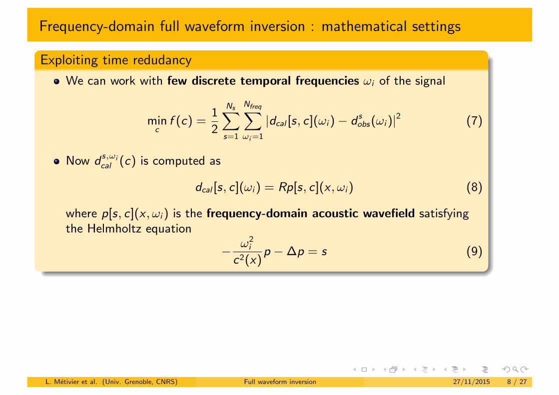
Frequency-domain full waveform inversion : mathematical settings
Exploiting time redudancy
We can work with few discrete temporal frequencies !i of the signal
minc
f (c) =12
NsX
s=1
NfreqX
!i =1
|dcal [s, c](!i )� d sobs(!i )|2 (7)
Now d s,!ical (c) is computed as
dcal [s, c](!i ) = Rp[s, c](x , !i ) (8)
where p[s, c](x , !i ) is the frequency-domain acoustic wavefield satisfyingthe Helmholtz equation
� !2i
c2(x)p ��p = s (9)
L. Metivier et al. (Univ. Grenoble, CNRS) Full waveform inversion 27/11/2015 8 / 27
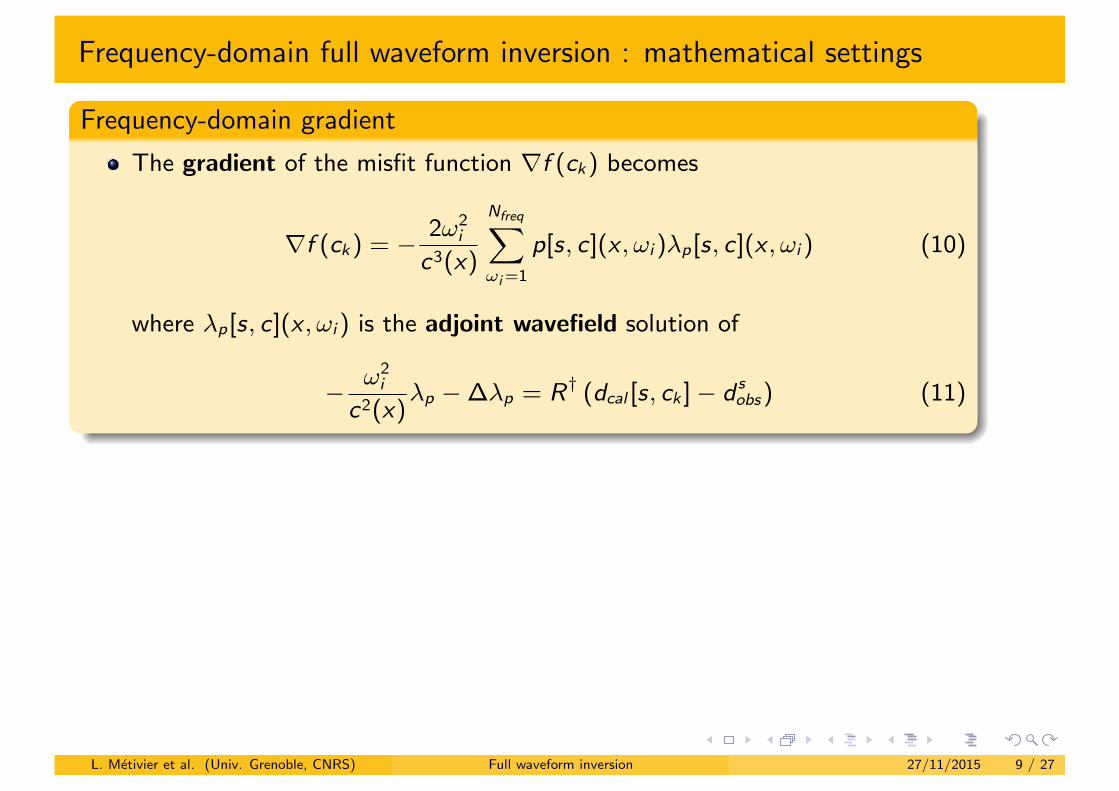
Frequency-domain full waveform inversion : mathematical settings
Frequency-domain gradient
The gradient of the misfit function rf (ck) becomes
rf (ck) = � 2!2i
c3(x)
NfreqX
!i =1
p[s, c](x , !i )�p[s, c](x , !i ) (10)
where �p[s, c](x , !i ) is the adjoint wavefield solution of
� !2i
c2(x)�p ���p = R† (dcal [s, ck ]� d s
obs) (11)
L. Metivier et al. (Univ. Grenoble, CNRS) Full waveform inversion 27/11/2015 9 / 27
Outline
1 Introduction: principle of full waveform inversion
2 Example of application: 3D acoustic frequency-domain FWI
3 Reducing the sensitivity to the initial model accuracy using an optimal transport distance
L. Metivier et al. (Univ. Grenoble, CNRS) Full waveform inversion 27/11/2015 10 / 27
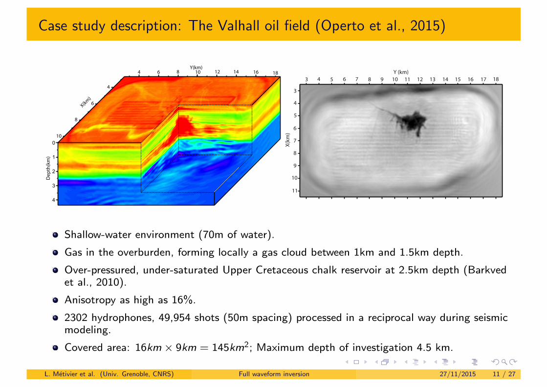
Case study description: The Valhall oil field (Operto et al., 2015)
0
1
2
3
4
4 6 8 10 12 14 16 18
4
6
8
10
Y(km)
X(km)
Dep
th(k
m)
Y (km)
3
4
5
6
7
8
9
10
11
3 4 5 6 7 8 9 10 11 12 13 14 15 16 17 18
X(km
)
Shallow-water environment (70m of water).
Gas in the overburden, forming locally a gas cloud between 1km and 1.5km depth.
Over-pressured, under-saturated Upper Cretaceous chalk reservoir at 2.5km depth (Barkvedet al., 2010).
Anisotropy as high as 16%.
2302 hydrophones, 49,954 shots (50m spacing) processed in a reciprocal way during seismicmodeling.
Covered area: 16km ⇥ 9km = 145km2; Maximum depth of investigation 4.5 km.
L. Metivier et al. (Univ. Grenoble, CNRS) Full waveform inversion 27/11/2015 11 / 27
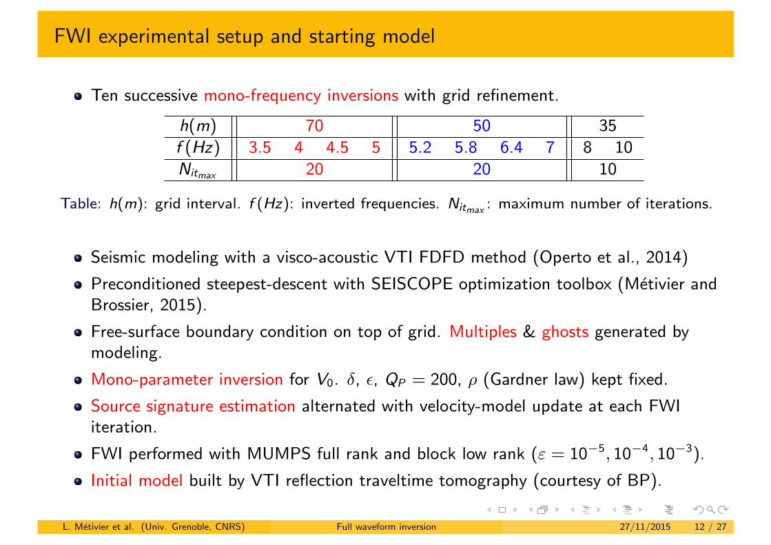
FWI experimental setup and starting model
Ten successive mono-frequency inversions with grid refinement.
h(m) 70 50 35f (Hz) 3.5 4 4.5 5 5.2 5.8 6.4 7 8 10Nitmax 20 20 10
Table: h(m): grid interval. f (Hz): inverted frequencies. Nitmax : maximum number of iterations.
Seismic modeling with a visco-acoustic VTI FDFD method (Operto et al., 2014)
Preconditioned steepest-descent with SEISCOPE optimization toolbox (Metivier andBrossier, 2015).
Free-surface boundary condition on top of grid. Multiples & ghosts generated bymodeling.
Mono-parameter inversion for V0. �, ✏, QP = 200, ⇢ (Gardner law) kept fixed.
Source signature estimation alternated with velocity-model update at each FWIiteration.
FWI performed with MUMPS full rank and block low rank (" = 10�5, 10�4, 10�3).
Initial model built by VTI reflection traveltime tomography (courtesy of BP).
L. Metivier et al. (Univ. Grenoble, CNRS) Full waveform inversion 27/11/2015 12 / 27
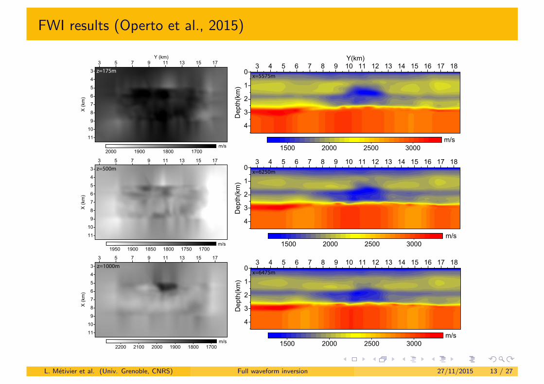
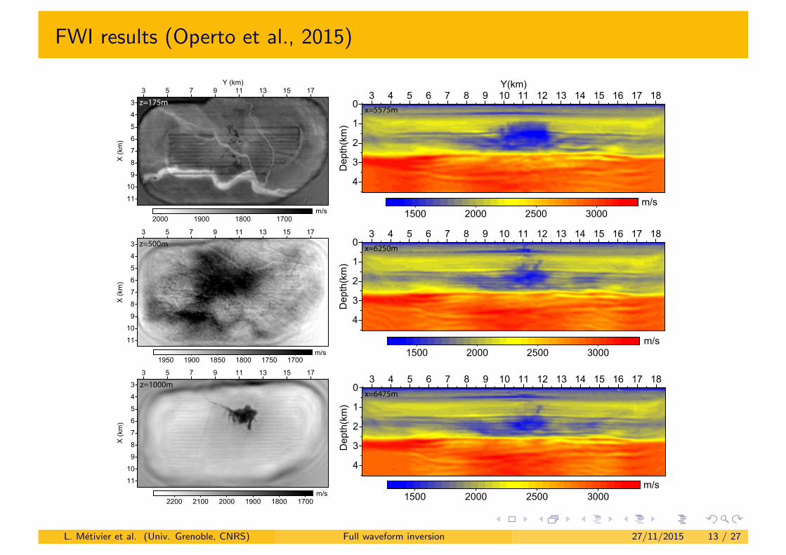
FWI results (Operto et al., 2015)
3
4
5
6
7
8
9
10
11
X (k
m)
3 5 7 9 11 13 15 17Y (km)
1700180019002000m/s
3
4
5
6
7
8
9
10
11
X (k
m)
3 5 7 9 11 13 15 17
170017501800185019001950m/s
3
4
5
6
7
8
9
10
11
X (k
m)
3 5 7 9 11 13 15 17
170018001900200021002200m/s
0
1
2
3
4
Dep
th(k
m)
3 4 5 6 7 8 9 10 11 12 13 14 15 16 17 18Y(km)
1500 2000 2500 3000m/s
0
1
2
3
4
Dep
th(k
m)
3 4 5 6 7 8 9 10 11 12 13 14 15 16 17 18
1500 2000 2500 3000m/s
0
1
2
3
4
Dep
th(k
m)
3 4 5 6 7 8 9 10 11 12 13 14 15 16 17 18
1500 2000 2500 3000m/s
z=175m
z=500m
z=1000m
x=5575m
x=6250m
x=6475m
L. Metivier et al. (Univ. Grenoble, CNRS) Full waveform inversion 27/11/2015 13 / 27

HPC strategy
Each inversion iteration requires to solve more than 2⇥ 2000 wave equationproblems with the same operator and di↵erent right hand sides (sources)
The total number of inversion iterations reaches 200 which makes 8⇥ 105
wave propagation problems solution for one inversion
We would like to rely on e�cient strategies for multiple right hand sidesproblems
We should use a direct solver
L. Metivier et al. (Univ. Grenoble, CNRS) Full waveform inversion 27/11/2015 14 / 27
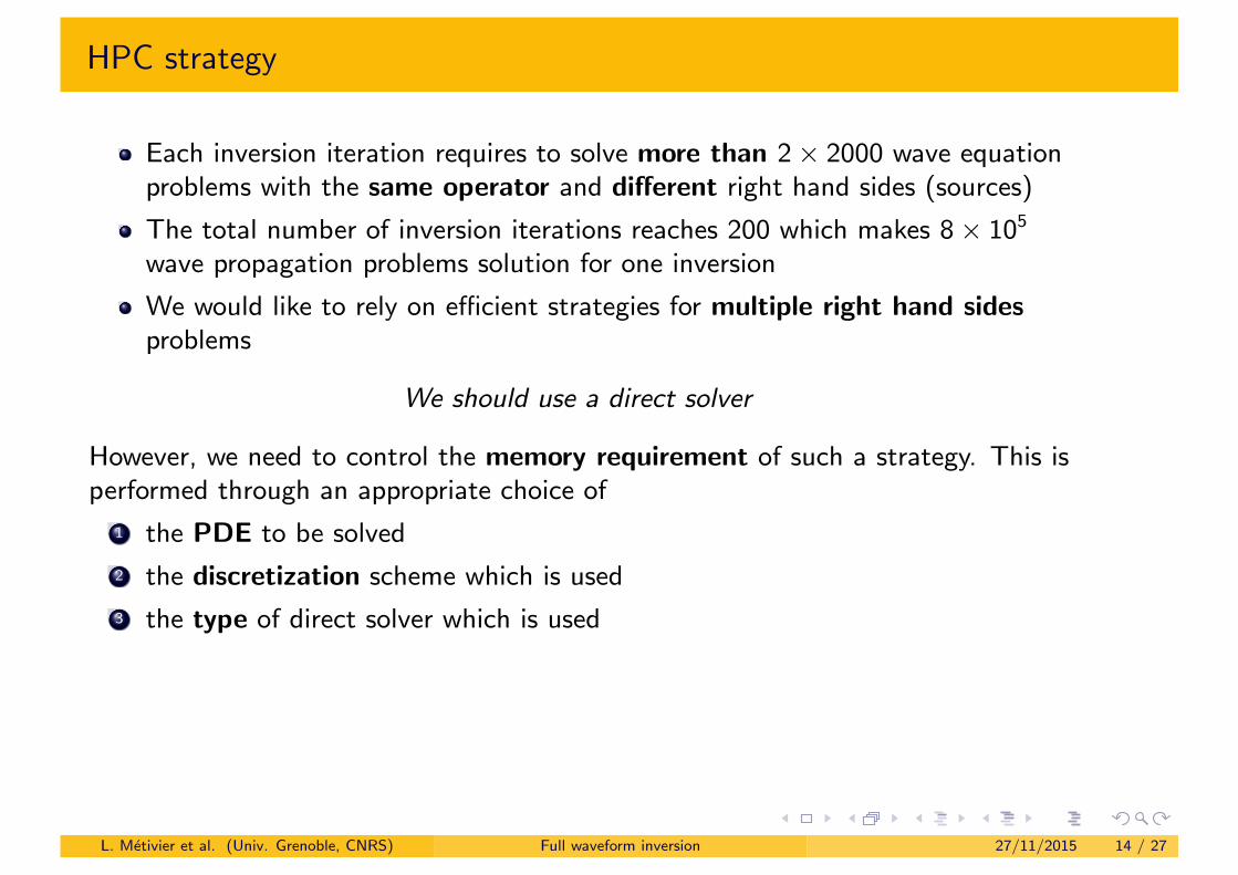
HPC strategy
Each inversion iteration requires to solve more than 2⇥ 2000 wave equationproblems with the same operator and di↵erent right hand sides (sources)
The total number of inversion iterations reaches 200 which makes 8⇥ 105
wave propagation problems solution for one inversion
We would like to rely on e�cient strategies for multiple right hand sidesproblems
We should use a direct solver
However, we need to control the memory requirement of such a strategy. This isperformed through an appropriate choice of
1 the PDE to be solved
2 the discretization scheme which is used
3 the type of direct solver which is used
L. Metivier et al. (Univ. Grenoble, CNRS) Full waveform inversion 27/11/2015 14 / 27
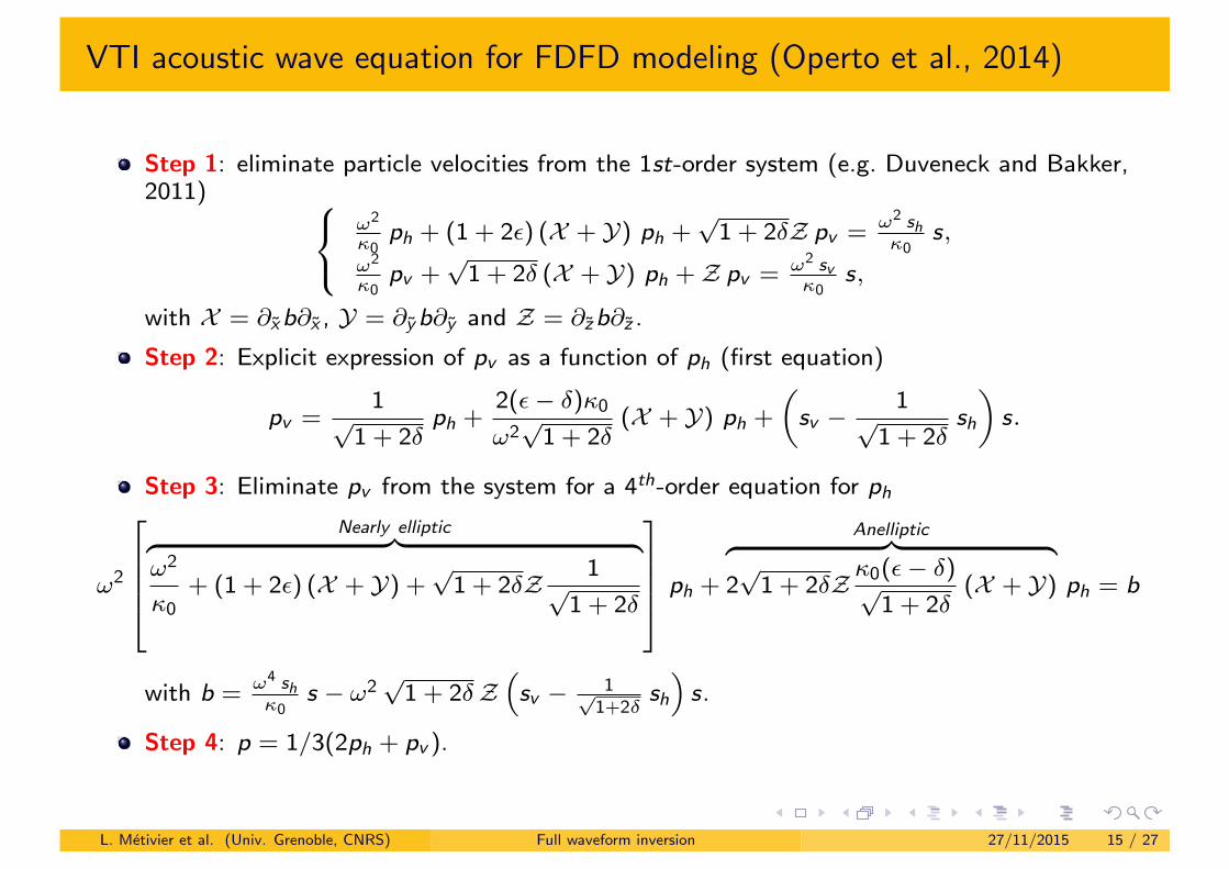
VTI acoustic wave equation for FDFD modeling (Operto et al., 2014)
Step 1: eliminate particle velocities from the 1st-order system (e.g. Duveneck and Bakker,2011) 8
<
:
!2
0ph + (1 + 2✏) (X + Y) ph +
p1 + 2�Z pv = !2 sh
0s,
!2
0pv +
p1 + 2� (X + Y) ph + Z pv = !2 sv
0s,
with X = @x b@x , Y = @y b@y and Z = @z b@z .
Step 2: Explicit expression of pv as a function of ph (first equation)
pv =1
p1 + 2�
ph +2(✏� �)0
!2p
1 + 2�(X + Y) ph +
„sv �
1p
1 + 2�sh
«s.
Step 3: Eliminate pv from the system for a 4th-order equation for ph
!2
2
6664
Nearly ellipticz }| {!2
0+ (1 + 2✏) (X + Y) +
p1 + 2�Z
1p
1 + 2�
3
7775ph +
Anellipticz }| {
2p
1 + 2�Z0(✏� �)p
1 + 2�(X + Y) ph = b
with b = !4 sh0
s � !2p
1 + 2�Z“sv � 1p
1+2�sh
”s.
Step 4: p = 1/3(2ph + pv ).
L. Metivier et al. (Univ. Grenoble, CNRS) Full waveform inversion 27/11/2015 15 / 27
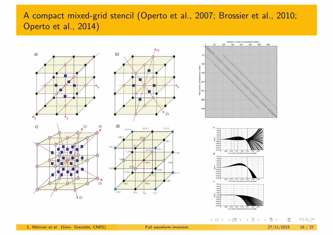
A compact mixed-grid stencil (Operto et al., 2007; Brossier et al., 2010;Operto et al., 2014)
L. Metivier et al. (Univ. Grenoble, CNRS) Full waveform inversion 27/11/2015 16 / 27
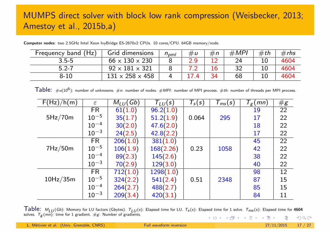
MUMPS direct solver with block low rank compression (Weisbecker, 2013;Amestoy et al., 2015b,a)
Computer nodes: two 2.5GHz Intel Xeon IvyBridge E5-2670v2 CPUs. 10 cores/CPU. 64GB memory/node.
Frequency band (Hz) Grid dimensions npml #u #n #MPI #th #rhs3.5-5 66 x 130 x 230 8 2.9 12 24 10 46045.2-7 92 x 181 x 321 8 7.2 16 32 10 46048-10 131 x 258 x 458 4 17.4 34 68 10 4604
Table: #u(106): number of unknowns. #n: number of nodes. #MPI : number of MPI process. #th: number of threads per MPI process.
F(Hz)/h(m) " MLU(Gb) TLU(s) Ts(s) Tms(s) Tg (mn) #g
5Hz/70mFR 61(1.0) 96.2(1.0) 19 22
10�5 35(1.7) 51.2(1.9) 0.064 295 17 2210�4 30(2.0) 47.6(2.0) 18 2210�3 24(2.5) 42.8(2.2) 17 22
7Hz/50mFR 206(1.0) 381(1.0) 45 22
10�5 106(1.9) 168(2.26) 0.23 1058 42 2210�4 89(2.3) 145(2.6) 38 2210�3 70(2.9) 129(3.0) 40 22
10Hz/35mFR 712(1.0) 1298(1.0) 98 12
10�5 324(2.2) 541(2.4) 0.51 2348 87 1510�4 264(2.7) 488(2.7) 85 1510�3 209(3.4) 420(3.1) 84 11
Table: MLU (Gb): Memory for LU factors (Gbytes). TLU (s): Elapsed time for LU. Ts (s): Elapsed time for 1 solve. Tms (s): Elapsed time for 4604solves. Tg (mn): time for 1 gradient. #g : Number of gradients.
L. Metivier et al. (Univ. Grenoble, CNRS) Full waveform inversion 27/11/2015 17 / 27
Outline
1 Introduction: principle of full waveform inversion
2 Example of application: 3D acoustic frequency-domain FWI
3 Reducing the sensitivity to the initial model accuracy using an optimal transport distance
L. Metivier et al. (Univ. Grenoble, CNRS) Full waveform inversion 27/11/2015 18 / 27
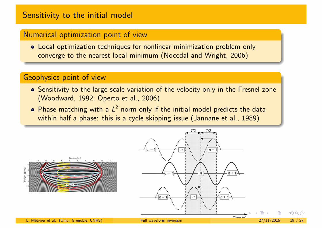
Sensitivity to the initial model
Numerical optimization point of view
Local optimization techniques for nonlinear minimization problem onlyconverge to the nearest local minimum (Nocedal and Wright, 2006)
Geophysics point of view
Sensitivity to the large scale variation of the velocity only in the Fresnel zone(Woodward, 1992; Operto et al., 2006)
Phase matching with a L2 norm only if the initial model predicts the datawithin half a phase: this is a cycle skipping issue (Jannane et al., 1989)
L. Metivier et al. (Univ. Grenoble, CNRS) Full waveform inversion 27/11/2015 19 / 27
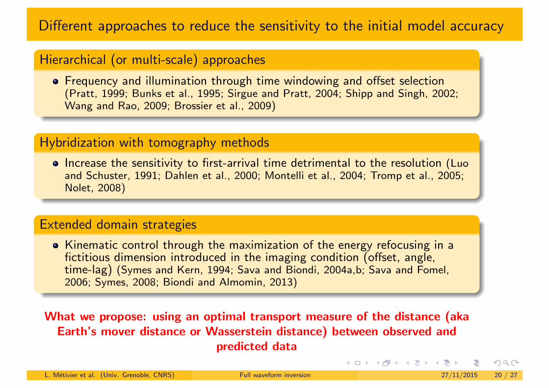
Di↵erent approaches to reduce the sensitivity to the initial model accuracy
Hierarchical (or multi-scale) approaches
Frequency and illumination through time windowing and o↵set selection(Pratt, 1999; Bunks et al., 1995; Sirgue and Pratt, 2004; Shipp and Singh, 2002;Wang and Rao, 2009; Brossier et al., 2009)
Hybridization with tomography methods
Increase the sensitivity to first-arrival time detrimental to the resolution (Luoand Schuster, 1991; Dahlen et al., 2000; Montelli et al., 2004; Tromp et al., 2005;Nolet, 2008)
Extended domain strategies
Kinematic control through the maximization of the energy refocusing in afictitious dimension introduced in the imaging condition (o↵set, angle,time-lag) (Symes and Kern, 1994; Sava and Biondi, 2004a,b; Sava and Fomel,2006; Symes, 2008; Biondi and Almomin, 2013)
L. Metivier et al. (Univ. Grenoble, CNRS) Full waveform inversion 27/11/2015 20 / 27
Di↵erent approaches to reduce the sensitivity to the initial model accuracy
Hierarchical (or multi-scale) approaches
Frequency and illumination through time windowing and o↵set selection(Pratt, 1999; Bunks et al., 1995; Sirgue and Pratt, 2004; Shipp and Singh, 2002;Wang and Rao, 2009; Brossier et al., 2009)
Hybridization with tomography methods
Increase the sensitivity to first-arrival time detrimental to the resolution (Luoand Schuster, 1991; Dahlen et al., 2000; Montelli et al., 2004; Tromp et al., 2005;Nolet, 2008)
Extended domain strategies
Kinematic control through the maximization of the energy refocusing in afictitious dimension introduced in the imaging condition (o↵set, angle,time-lag) (Symes and Kern, 1994; Sava and Biondi, 2004a,b; Sava and Fomel,2006; Symes, 2008; Biondi and Almomin, 2013)
What we propose: using an optimal transport measure of the distance (akaEarth’s mover distance or Wasserstein distance) between observed and
predicted data
L. Metivier et al. (Univ. Grenoble, CNRS) Full waveform inversion 27/11/2015 20 / 27
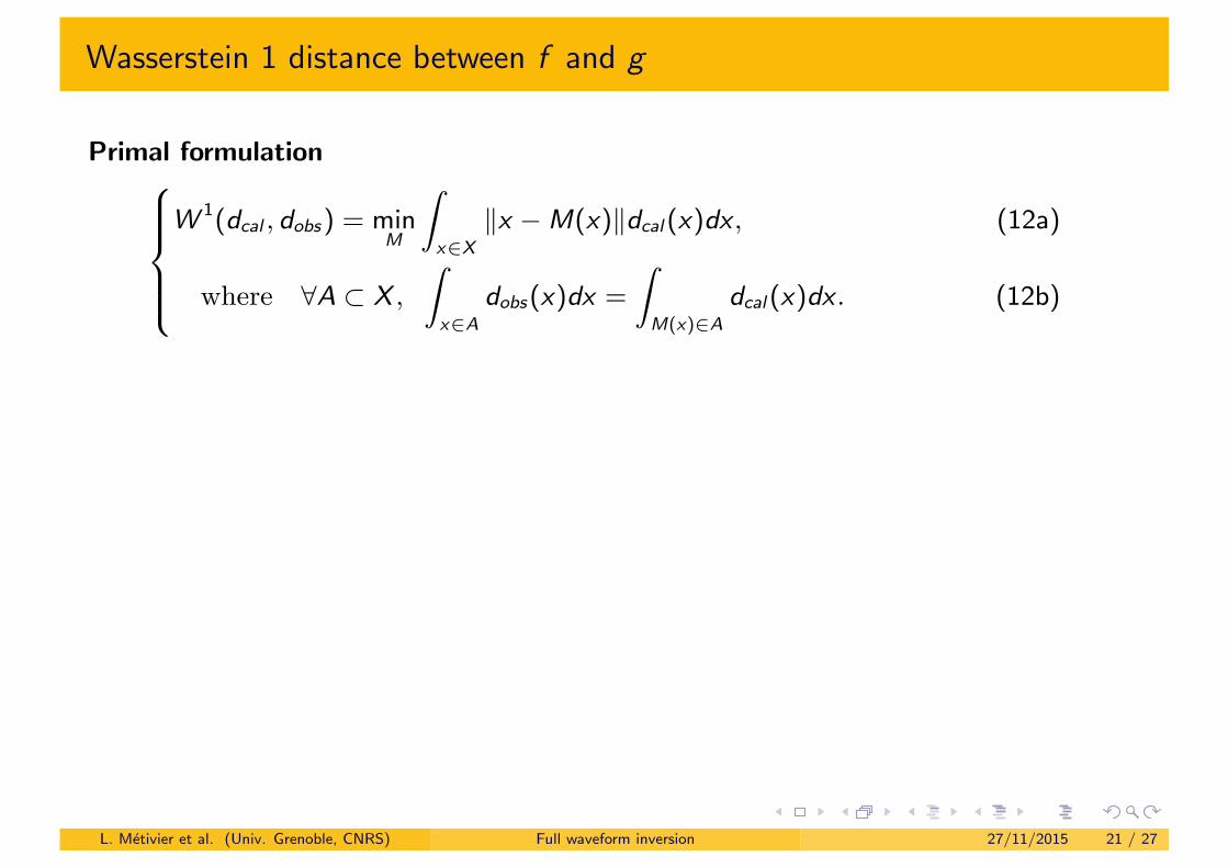
Wasserstein 1 distance between f and g
Primal formulation8
>
>
>
<
>
>
>
:
W 1(dcal , dobs) = minM
Z
x2X
kx �M(x)kdcal(x)dx ,
where 8A ⇢ X ,
Z
x2A
dobs(x)dx =
Z
M(x)2A
dcal(x)dx .
(12a)
(12b)
L. Metivier et al. (Univ. Grenoble, CNRS) Full waveform inversion 27/11/2015 21 / 27

Wasserstein 1 distance between f and g
Primal formulation8
>
>
>
<
>
>
>
:
W 1(dcal , dobs) = minM
Z
x2X
kx �M(x)kdcal(x)dx ,
where 8A ⇢ X ,
Z
x2A
dobs(x)dx =
Z
M(x)2A
dcal(x)dx .
(12a)
(12b)
Dual equivalent formulation
W 1 (dcal , dobs) = max' 2Lip1
Z
x2X
'(x) (dcal(x)� dobs(x)) dx , (13)
where Lip1 is the space of 1-Lipschitz functions, such that
8(x , y) 2 X , |'(x)� '(y)| kx � yk1. (14)
L. Metivier et al. (Univ. Grenoble, CNRS) Full waveform inversion 27/11/2015 21 / 27
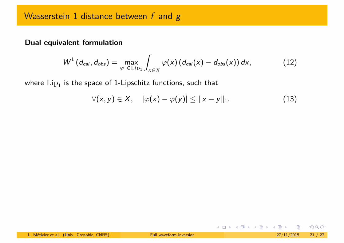
Wasserstein 1 distance between f and g
Dual equivalent formulation
W 1 (dcal , dobs) = max' 2Lip1
Z
x2X
'(x) (dcal(x)� dobs(x)) dx , (12)
where Lip1 is the space of 1-Lipschitz functions, such that
8(x , y) 2 X , |'(x)� '(y)| kx � yk1. (13)
L. Metivier et al. (Univ. Grenoble, CNRS) Full waveform inversion 27/11/2015 21 / 27
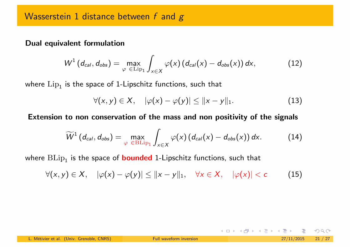
Wasserstein 1 distance between f and g
Dual equivalent formulation
W 1 (dcal , dobs) = max' 2Lip1
Z
x2X
'(x) (dcal(x)� dobs(x)) dx , (12)
where Lip1 is the space of 1-Lipschitz functions, such that
8(x , y) 2 X , |'(x)� '(y)| kx � yk1. (13)
Extension to non conservation of the mass and non positivity of the signals
fW 1 (dcal , dobs) = max' 2BLip1
Z
x2X
'(x) (dcal(x)� dobs(x)) dx . (14)
where BLip1 is the space of bounded 1-Lipschitz functions, such that
8(x , y) 2 X , |'(x)� '(y)| kx � yk1, 8x 2 X , |'(x)| < c (15)
L. Metivier et al. (Univ. Grenoble, CNRS) Full waveform inversion 27/11/2015 21 / 27
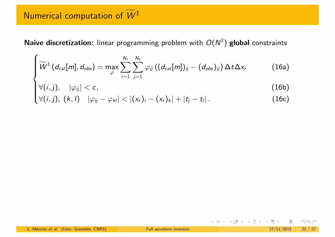
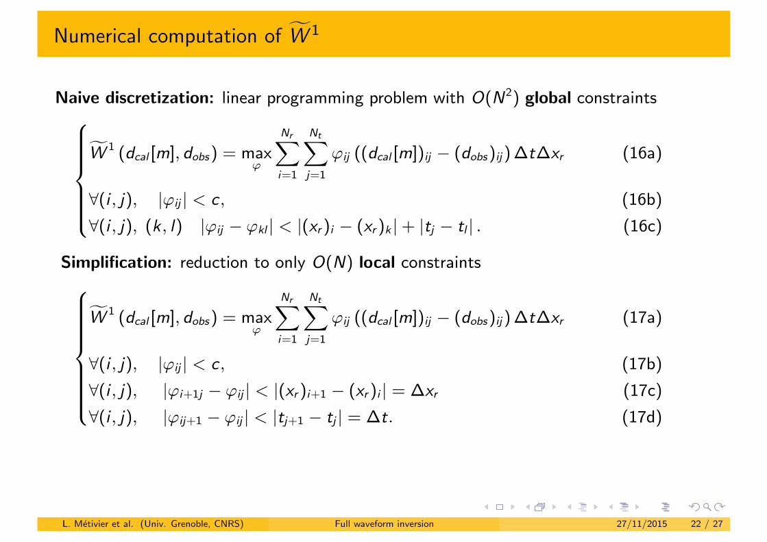
Numerical computation of fW 1
Naive discretization: linear programming problem with O(N2) global constraints8
>
>
>
>
>
<
>
>
>
>
>
:
fW 1 (dcal [m], dobs) = max'
NrX
i=1
NtX
j=1
'ij ((dcal [m])ij � (dobs)ij)�t�xr
8(i , j), |'ij | < c,
8(i , j), (k, l) |'ij � 'kl | < |(xr )i � (xr )k | + |tj � tl | .
(16a)
(16b)
(16c)
L. Metivier et al. (Univ. Grenoble, CNRS) Full waveform inversion 27/11/2015 22 / 27
Numerical computation of fW 1
Naive discretization: linear programming problem with O(N2) global constraints8
>
>
>
>
>
<
>
>
>
>
>
:
fW 1 (dcal [m], dobs) = max'
NrX
i=1
NtX
j=1
'ij ((dcal [m])ij � (dobs)ij)�t�xr
8(i , j), |'ij | < c,
8(i , j), (k, l) |'ij � 'kl | < |(xr )i � (xr )k | + |tj � tl | .
(16a)
(16b)
(16c)
Simplification: reduction to only O(N) local constraints
8
>
>
>
>
>
>
>
<
>
>
>
>
>
>
>
:
fW 1 (dcal [m], dobs) = max'
NrX
i=1
NtX
j=1
'ij ((dcal [m])ij � (dobs)ij)�t�xr
8(i , j), |'ij | < c,
8(i , j), |'i+1j � 'ij | < |(xr )i+1 � (xr )i | = �xr
8(i , j), |'ij+1 � 'ij | < |tj+1 � tj | = �t.
(17a)
(17b)
(17c)
(17d)
L. Metivier et al. (Univ. Grenoble, CNRS) Full waveform inversion 27/11/2015 22 / 27
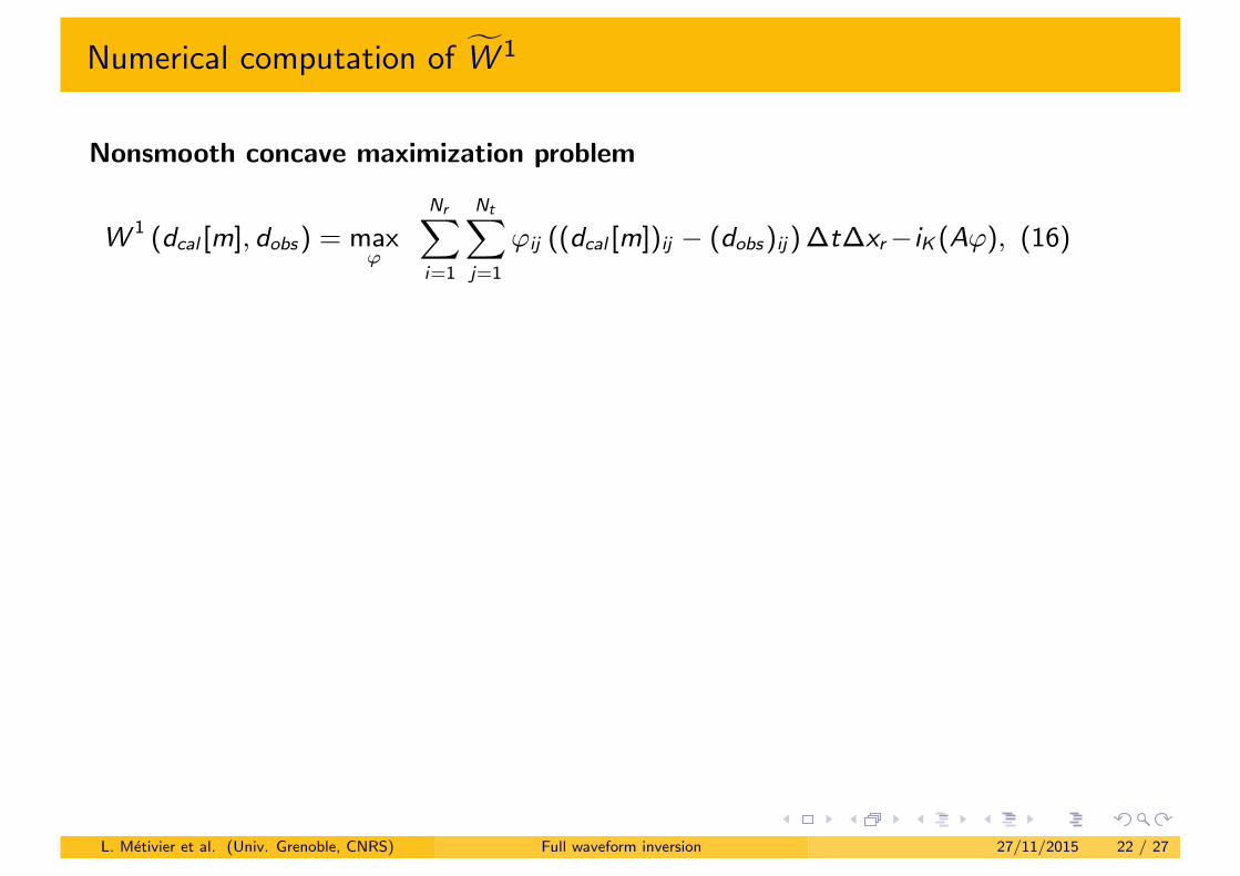
Numerical computation of fW 1
Nonsmooth concave maximization problem
W 1 (dcal [m], dobs) = max'
NrX
i=1
NtX
j=1
'ij ((dcal [m])ij � (dobs)ij)�t�xr�iK (A'), (16)
L. Metivier et al. (Univ. Grenoble, CNRS) Full waveform inversion 27/11/2015 22 / 27
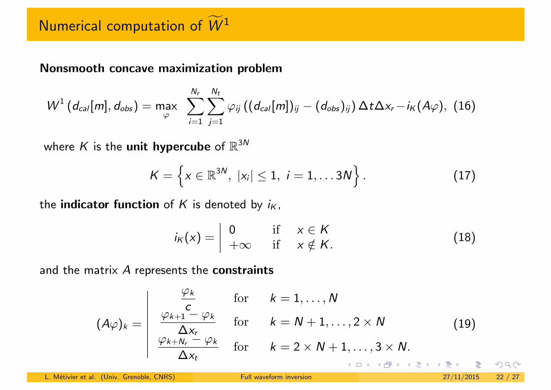
Numerical computation of fW 1
Nonsmooth concave maximization problem
W 1 (dcal [m], dobs) = max'
NrX
i=1
NtX
j=1
'ij ((dcal [m])ij � (dobs)ij)�t�xr�iK (A'), (16)
where K is the unit hypercube of R3N
K =n
x 2 R3N , |xi | 1, i = 1, . . . 3No
. (17)
the indicator function of K is denoted by iK ,
iK (x) =
˛
˛
˛
˛
0 if x 2 K+1 if x /2 K .
(18)
and the matrix A represents the constraints
(A')k =
˛
˛
˛
˛
˛
˛
˛
˛
˛
'k
cfor k = 1, . . . , N
'k+1 � 'k
�xrfor k = N + 1, . . . , 2⇥ N
'k+Nr � 'k
�xtfor k = 2⇥ N + 1, . . . , 3⇥ N.
(19)
L. Metivier et al. (Univ. Grenoble, CNRS) Full waveform inversion 27/11/2015 22 / 27
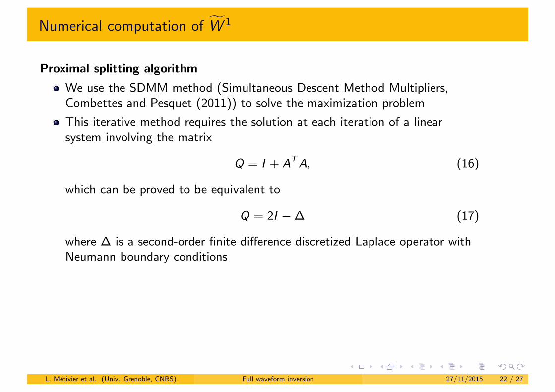
Numerical computation of fW 1
Proximal splitting algorithm
We use the SDMM method (Simultaneous Descent Method Multipliers,Combettes and Pesquet (2011)) to solve the maximization problem
This iterative method requires the solution at each iteration of a linearsystem involving the matrix
Q = I + ATA, (16)
which can be proved to be equivalent to
Q = 2I �� (17)
where � is a second-order finite di↵erence discretized Laplace operator withNeumann boundary conditions
L. Metivier et al. (Univ. Grenoble, CNRS) Full waveform inversion 27/11/2015 22 / 27
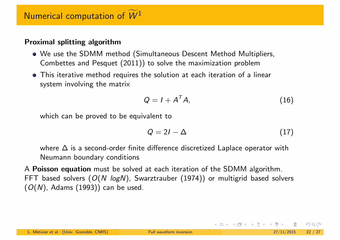
Numerical computation of fW 1
Proximal splitting algorithm
We use the SDMM method (Simultaneous Descent Method Multipliers,Combettes and Pesquet (2011)) to solve the maximization problem
This iterative method requires the solution at each iteration of a linearsystem involving the matrix
Q = I + ATA, (16)
which can be proved to be equivalent to
Q = 2I �� (17)
where � is a second-order finite di↵erence discretized Laplace operator withNeumann boundary conditions
A Poisson equation must be solved at each iteration of the SDMM algorithm.FFT based solvers (O(N logN), Swarztrauber (1974)) or multigrid based solvers(O(N), Adams (1993)) can be used.
L. Metivier et al. (Univ. Grenoble, CNRS) Full waveform inversion 27/11/2015 22 / 27
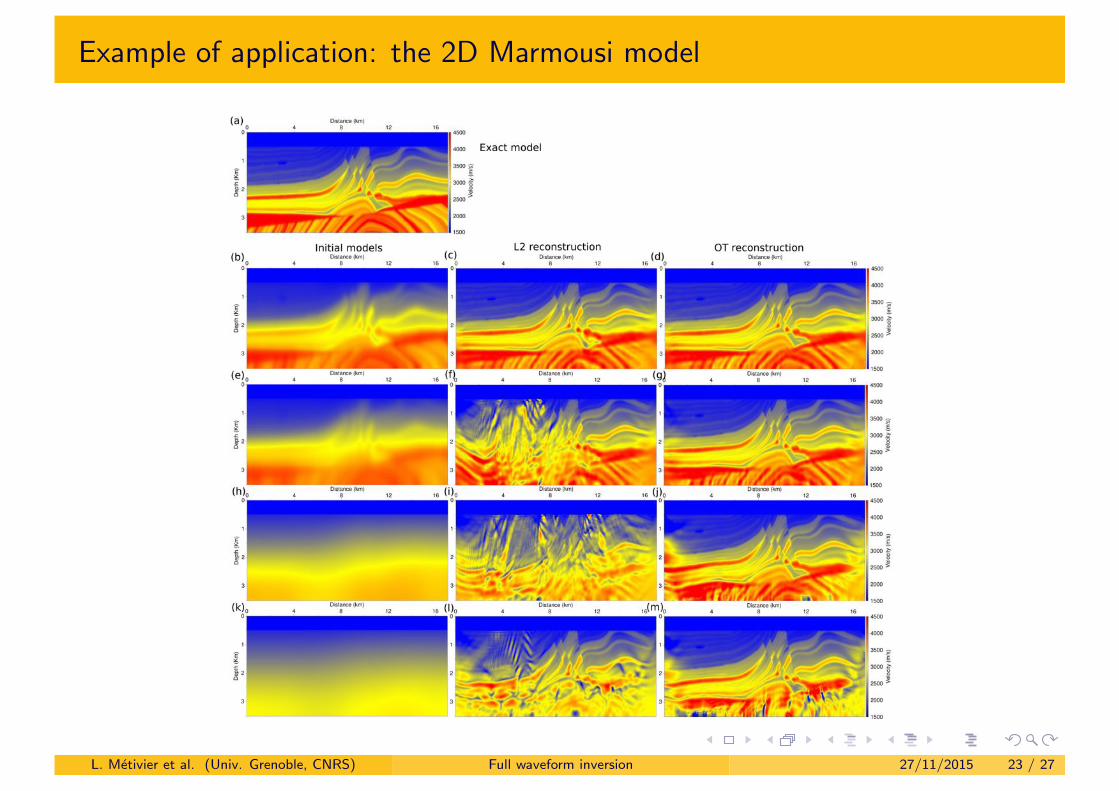
Example of application: the 2D Marmousi model
L. Metivier et al. (Univ. Grenoble, CNRS) Full waveform inversion 27/11/2015 23 / 27

Marmousi 2 iterative reconstruction using a L2 distance
L. Metivier et al. (Univ. Grenoble, CNRS) Full waveform inversion 27/11/2015 24 / 27
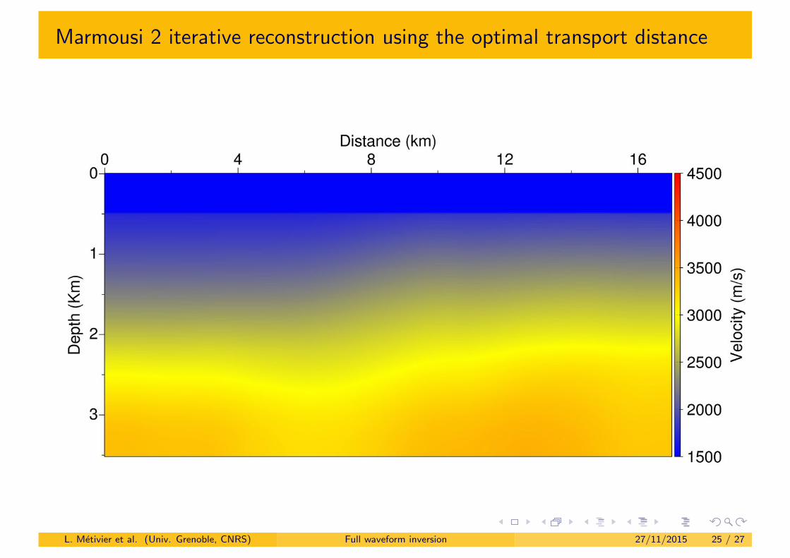
Marmousi 2 iterative reconstruction using the optimal transport distance
L. Metivier et al. (Univ. Grenoble, CNRS) Full waveform inversion 27/11/2015 25 / 27

Conclusion and perspectives
A direct solver strategy amenable for moderate size 3D acoustic problems
Frequency-domain strategies with sparse direct solvers are amenable for moderatesize 3D acoustic problems using appropriate choice of PDE, discretized scheme,and solver
Low rank compression will help us push up the limit of this strategy (Amestoyet al., 2015a), however 3D elastodynamics still seems out of reach: time-domainmethods are still preferred for this problem
Beyond the L2 distance: mitigating the sensitivity to the initial model accuracy
Standard FWI still relies on the assumption that the initial model is accurateenough: the sensitivity to the accuracy of the initial model could be mitigated bythe choice of an optimal transport distance instead of the standard L2 norm(Metivier et al., 2016)
L. Metivier et al. (Univ. Grenoble, CNRS) Full waveform inversion 27/11/2015 26 / 27
Acknowledgments
Thank you for your attention
National HPC facilities of GENCI-IDRIS under grant Grant 046091
Local HPC facilities of CIMENT-SCCI (Univ. Grenoble)
SEICOPE sponsors : http://seiscope2.osug.fr
L. Metivier et al. (Univ. Grenoble, CNRS) Full waveform inversion 27/11/2015 27 / 27
Adams, J. C. (1993). Mudpack-2: multigrid software for approximating elliptic partial di↵erential equations onuniform grids with any resolution. Applied Mathematics and Computation.
Amestoy, P., , Brossier, R., Buttari, A., L’Excellent, J.-Y., Mary, T., Metivier, L., Miniussi, A., Operto, S.,Virieux, J., and Weisbecker, C. (2015a). 3d frequency-domain seismic modeling with a parallel blrmultifrontal direct solver. In Expanded Abstracts, 85th Annual SEG Meeting (New Orleans).
Amestoy, P. R., Ashcraft, C., Boiteau, O., Buttari, A., L’Excellent, J.-Y., and Weisbecker, C. (2015b).Improving multifrontal methods by means of block low-rank representations. SIAM Journal on ScientificComputing, 37(3):1451–1474.
Barkved, O., Albertin, U., Heavey, P., Kommedal, J., van Gestel, J., Synnove, R., Pettersen, H., and Kent, C.(2010). Business impact of full waveform inversion at Valhall. In Expanded Abstracts, 91 Annual SEGMeeting and Exposition (October 17-22, Denver), pages 925–929. Society of Exploration Geophysics.
Biondi, B. and Almomin, A. (2013). Tomographic full waveform inversion (TFWI) by combining FWI andwave-equation migration velocity analysis. The Leading Edge, September, special section: full waveforminversion:1074–1080.
Brossier, R., Etienne, V., Operto, S., and Virieux, J. (2010). Frequency-domain numerical modelling ofvisco-acoustic waves based on finite-di↵erence and finite-element discontinuous galerkin methods. InDissanayake, D. W., editor, Acoustic Waves, pages 125–158. SCIYO.
Brossier, R., Operto, S., and Virieux, J. (2009). Seismic imaging of complex onshore structures by 2D elasticfrequency-domain full-waveform inversion. Geophysics, 74(6):WCC105–WCC118.
Bunks, C., Salek, F. M., Zaleski, S., and Chavent, G. (1995). Multiscale seismic waveform inversion.Geophysics, 60(5):1457–1473.
Combettes, P. L. and Pesquet, J.-C. (2011). Proximal splitting methods in signal processing. In Bauschke,H. H., Burachik, R. S., Combettes, P. L., Elser, V., Luke, D. R., and Wolkowicz, H., editors, Fixed-PointAlgorithms for Inverse Problems in Science and Engineering, volume 49 of Springer Optimization and ItsApplications, pages 185–212. Springer New York.
Dahlen, F. A., Hung, S. H., and Nolet, G. (2000). Frechet kernels for finite-di↵erence traveltimes - I. theory.Geophysical Journal International, 141:157–174.
Duveneck, E. and Bakker, P. M. (2011). Stable P-wave modeling for reverse-time migration in tilted TI media.Geophysics, 76(2):S65–S75.
L. Metivier et al. (Univ. Grenoble, CNRS) Full waveform inversion 27/11/2015 27 / 27
Jannane, M., Beydoun, W., Crase, E., Cao, D., Koren, Z., Landa, E., Mendes, M., Pica, A., Noble, M., Roeth,G., Singh, S., Snieder, R., Tarantola, A., and Trezeguet, D. (1989). Wavelengths of Earth structures thatcan be resolved from seismic reflection data. Geophysics, 54(7):906–910.
Luo, Y. and Schuster, G. T. (1991). Wave-equation traveltime inversion. Geophysics, 56(5):645–653.
Metivier, L. and Brossier, R. (2015). The seiscope optimization toolbox: A large-scale nonlinear optimizationlibrary based on reverse communication. Geophysics, pages in–press.
Metivier, L., Brossier, R., Merigot, Q., Oudet, E., and Virieux, J. (2016). Measuring the misfit betweenseismograms using an optimal transport distance: Application to full waveform inversion. GeophysicalJournal International, page submitted.
Montelli, R., Nolet, G., Dahlen, F. A., Masters, G., Engdahl, E. R., and Hung, S. H. (2004). Finite-frequencytomography reveals a variety of plumes in the mantle. Science, 303:338–343.
Nocedal, J. (1980). Updating Quasi-Newton Matrices With Limited Storage. Mathematics of Computation,35(151):773–782.
Nocedal, J. and Wright, S. J. (2006). Numerical Optimization. Springer, 2nd edition.
Nolet, G. (2008). A Breviary of Seismic Tomography. Cambridge University Press, Cambridge, UK.
Operto, S., Brossier, R., Combe, L., Metivier, L., Ribodetti, A., and Virieux, J. (2014).Computationally-e�cient three-dimensional visco-acoustic finite-di↵erence frequency-domain seismicmodeling in vertical transversely isotropic media with sparse direct solver. Geophysics, 79(5):T257–T275.
Operto, S., Miniussi, A., Brossier, R., Combe, L., Metivier, L., Monteiller, V., Ribodetti, A., and Virieux, J.(2015). E�cient 3-D frequency-domain mono-parameter full-waveform inversion of ocean-bottom cabledata: application to Valhall in the visco-acoustic vertical transverse isotropic approximation. GeophysicalJournal International, 202(2):1362–1391.
Operto, S., Virieux, J., Amestoy, P., L’Excellent, J.-Y., Giraud, L., and Ben Hadj Ali, H. (2007). 3Dfinite-di↵erence frequency-domain modeling of visco-acoustic wave propagation using a massively paralleldirect solver: A feasibility study. Geophysics, 72(5):SM195–SM211.
Operto, S., Virieux, J., Dessa, J. X., and Pascal, G. (2006). Crustal imaging from multifold ocean bottomseismometers data by frequency-domain full-waveform tomography: application to the eastern Nankaitrough. Journal of Geophysical Research, 111(B09306):doi:10.1029/2005JB003835.
L. Metivier et al. (Univ. Grenoble, CNRS) Full waveform inversion 27/11/2015 27 / 27
Pratt, R. G. (1999). Seismic waveform inversion in the frequency domain, part I : theory and verification in aphysic scale model. Geophysics, 64:888–901.
Sava, P. and Biondi, B. (2004a). Wave-equation migration velocity analysis. i. theory. GeophysicalProspecting, 52(6):593–606.
Sava, P. and Biondi, B. (2004b). Wave-equation migration velocity analysis. ii. subsalt imaging examples.Geophysical Prospecting, 52(6):607–623.
Sava, P. and Fomel, S. (2006). Time-shift imaging condition in seismic migration. Geophysics,71(6):S209–S217.
Shipp, R. M. and Singh, S. C. (2002). Two-dimensional full wavefield inversion of wide-aperture marine seismicstreamer data. Geophysical Journal International, 151:325–344.
Sirgue, L. and Pratt, R. G. (2004). E�cient waveform inversion and imaging : a strategy for selecting temporalfrequencies. Geophysics, 69(1):231–248.
Swarztrauber, P. N. (1974). A Direct Method for the Discrete Solution of Separable Elliptic Equations. SIAMJournal on Numerical Analysis, 11(6):1136–1150.
Symes, W. and Kern, M. (1994). Inversion of reflection seismograms by di↵erential semblance analysis:algorithm structure and synthetic examples. Geophysical Prospecting, 42:565–614.
Symes, W. W. (2008). Migration velocity analysis and waveform inversion. Geophysical Prospecting,56:765–790.
Tromp, J., Tape, C., and Liu, Q. (2005). Seismic tomography, adjoint methods, time reversal andbanana-doughnut kernels. Geophysical Journal International, 160:195–216.
Wang, Y. and Rao, Y. (2009). Reflection seismic waveform tomography. Journal of Geophysical Research,114(B03304):doi:10.1029/2008JB005916.
Weisbecker, C. (2013). Improving multifrontal solvers by means of algebraic Block Low-Rank representations.PhD thesis, Toulouse University, INP Toulouse.
Woodward, M. J. (1992). Wave-equation tomography. Geophysics, 57:15–26.
L. Metivier et al. (Univ. Grenoble, CNRS) Full waveform inversion 27/11/2015 27 / 27