Research Topic

Updated on Oct. 9, 2014

Wave Attenuation by Vegetation

Sponsored by SERRI, DHS

Lab/Field Experiments &

Computational Modeling

Ole Miss, LSU, NSL

2

Research Team

• PI: Dr. Weiming Wu

Computational modeling team:

• Dr. Weiming Wu, Dr. Yan Ding, Dr. S. N. Kuiry, Dr. Mingliang Zhang,

Mr. Reza Marsooli (NCCHE)

Laboratory experiment team:

• Dr. Daniel Wren (NSL), Dr. Yavuz Ozeren (NCCHE)

Field investigation team:

• Dr. Qin Chen, Dr. Guoping Zhang, Mr. Ranjit Jadhav, Mr. James

Chatagnier, Kyle Parker, James Bouanchaud, Hem Pant (LSU)

• Dr. Marjorie Holland, Miss Ying Chen (UM-Biology)

3

Laboratory and Field Experiments of

Wave Attenuation by Vegetation

(Project period: 2009-2012)

4

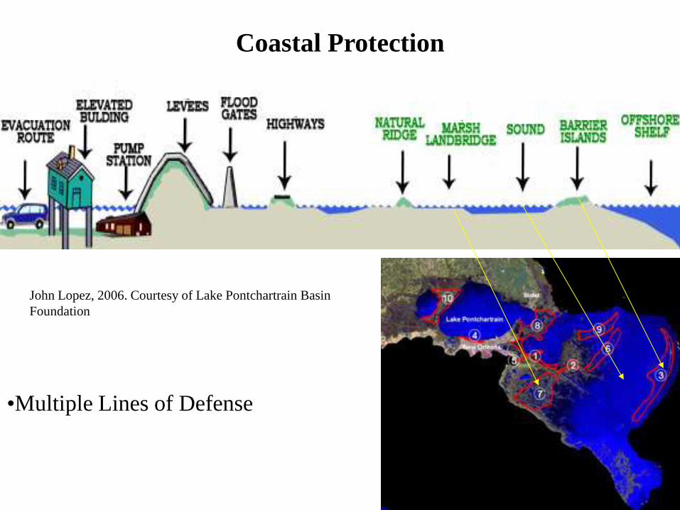
Coastal Protection

John Lopez, 2006. Courtesy of Lake Pontchartrain Basin

Foundation

•Multiple Lines of Defense

Surge/Wave vs. Vegetation

Vegetation attenuates waves and surge, while it is stressed by waves and surge.

6

Louisiana has lost 1,829 square miles of land since the 1930's (Barras et al. 2008, Britsch and

Dunbar 1993)

Marsh Edge Erosion by Waves and Surges

Between 1990 and 2001, wetland loss was approximately 13 square miles per year- that is the

equivalent of approximately one football field lost every hour (Barras et al. 2008). According to

land loss estimates, Hurricanes Katrina and Rita transformed 198 square miles of marsh to open

water in coastal Louisiana (Barras et al. 2008).

7

Spartina alterniflora Loisel.

http://plants.usda.gov/maps/large/SP/SPAL.png

Studied Vegetation Species I:

8

Spartina alterniflora at Terrebonne Bay, LA (4/4/2011)

Juncus roemerianus Scheele

Studied Vegetation Species II:

9

http://plants.usda.gov/core/profile?symbol=JURO

Smooth Cord Grass Bending Stiffness

• Measurement Procedure:

– Total plant height and stem height are measured

– A clip is attached at half the stem height

– Plants are pulled to a 45° angle

– Force needed is measured with a force gauge

– Plant is cut at base and maximum stem diameter is

measured

Diameter (D)

Height of Stem (H₁)

Height of Plant (H₂)

45°

Force (F)

10

Vegetation Properties

Plant Stiffness Modulus

Breton Sound

12

Zonation of eight experimental transects

at Grand Bay and Graveline Bayou, MS

(four coastal transects)

Zonation of eight experimental transects

at Grand Bay and Graveline Bayou, MS

(four inland transects)

Vegetation characteristics of low and high marsh

zones combined in eight transects

15

Short- term Rapid Deployment during Tropical Storm/

Hurricane

(Tropical Storm Ida Measurements)

• Landfall on Nov. 10, 2009 on the Mississippi coast

• Five wave gages were deployed by LSU on Nov. 9, 2009 in Breton Sound, LA

• All gages were retrieved after 11 days

• Measured waves and surge analyzed

16

Tropical Storm Ida Deployment –Gage Locations

F

Breton Sound

New Orleans

Five Wave and Surge Gages: J, F, I, E, G

17

J

F

I

E

Tropical Storm Ida:

Measured Wave Height Attenuation

Gage J – Gage F: Large Wave attenuation due to wave breaking and vegetation Gage F – Gage I: Wave attenuation by vegetation Gage I – Gage E: Milder wave attenuation rate by vegetation as wave height decreases.

18

TS Lee track

Gage locations Deployed on 3-Sep-2011; retrieved on 10-Sep-2011

Wave gages

Surge gages

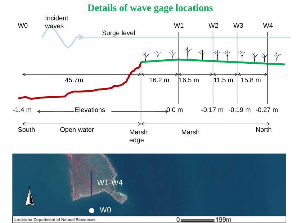
16.2 m 45.7m 16.5 m 11.5 m 15.8 m

W0 W1 W2 W3 W4

Marsh

edge

-1.4 m 0.0 m -0.17 m -0.19 m -0.27 m

Surge level

Marsh Open water North South

Elevations

Incident

waves

W0

W1-W4

Details of wave gage locations

Sample of simultaneous wave spectra recorded at 4 marsh gages 22

Spatial variation of measured wave heights at four marsh gages for various ranges of submergence

ratio, α, at gage W1. Number of records in each range is given by n. Symbols indicate mean values

and vertical bars are ±1 standard deviation. Using α from one gage only for classification ensures

that the same waves are followed across the transect to compute the mean.

23

Drag Force of Vegetation

1

2D D v v v vF C N A U U

0.5

vv v

hU U

h

For submerged vegetation, Stone and Shen’s (2002) method:

24

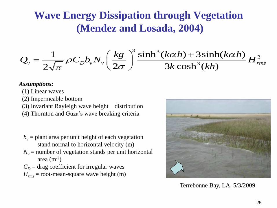
Wave Energy Dissipation through Vegetation

(Mendez and Losada, 2004)

3 33

3

1 sinh ( ) 3sinh( )

2 3 cosh ( )2v D v v rms

kg k h k hQ C b N H

k kh

bv = plant area per unit height of each vegetation

stand normal to horizontal velocity (m)

Nv = number of vegetation stands per unit horizontal

area (m-2)

CD = drag coefficient for irregular waves

Hrms = root-mean-square wave height (m)

Assumptions:

(1) Linear waves

(2) Impermeable bottom

(3) Invariant Rayleigh wave height distribution

(4) Thornton and Guza’s wave breaking criteria

Terrebonne Bay, LA, 5/3/2009

25

Estimated Vegetation Drag Coefficient Cd

using Dalrymple (1984)

26

Laboratory Experiments

27

Rigid Vegetation

Live Vegetation

Video

30

Video (Live Vegetation)

31

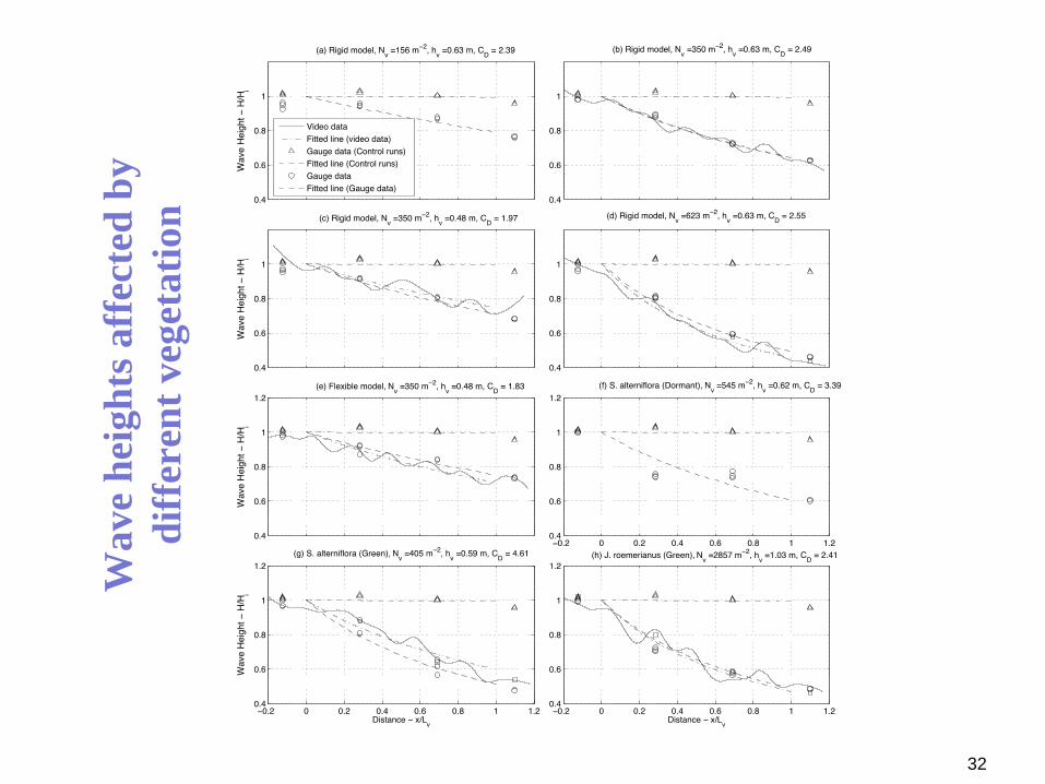
Wa

ve

hei

gh

ts a

ffec

ted

by

dif

fere

nt

veg

eta

tio

n

32

Average trends of the drag coefficient for rigid, flexible and live vegetation models under regular

waves. 33

Average trends of the drag coefficient for rigid, flexible and live vegetation models under

random waves. 34

Sloping Beach Experiments

0.69m

35

Wave Runup Experiment using Rigid Model

Vegetation

36

Flexible vegetation on sloping beach profile

Swash gauge

Wave Runup Experiment using Flexible Model

Vegetation

37

Flexible Model Vegetation

• Polyurethane tubing is the closest match to S. Alterniflora in terms of elastic properties when the model to prototype ratio is 1:3.

EPDM rubber Polyurethane Model Prototype

E (GPa) 3.86E-03 3.59E-02 9.46E-02 2.83E-01 (LSU team)

EI (Nt*m2) 1.60E-05 1.41E-04 1.17E-04 2.84E-02 (Feagin, 2010) 38

Computational Modeling of Wave

Attenuation by Vegetation

39

Models Used for Wave Attenuation

• 1-D/2-D shallow water flow models with HLL

approximate Riemann solver (Wu and Marsooli,

2012)

• 1-D Boussinesq wave model

• 2-D vertical Navier-Stokes model with VOF

• 3-D Navier-Stokes models with VOF (Marsooli and

Wu, 2014)

• 2-D spectral wave transformation model

• 3-D shallow water model coupled with spectral wave

transformation model (Wu, 2014)

40

Depth-Averaged 2-D Model for Long Waves

(Wu and Marsooli, 2012)

,

Governing equations:

0

Uh Vhh

t x y

2

2

1/3

1 bx t t

U U n m UUUh U h UVh F gh h h g

t x y x x x y y h

2

2

1/3

1 by t t

V V n m VUVh UVh V h F gh h h g

t x y y x x y y h

1

2

vii D v v vi vj vj M v v

UF C N A U U U C N V

t

Drag and inertia forces::

41

Drag Force of Submerged Vegetation

1

2D D v v v vF C N A U U

0.5

vv v

hU U

h

For submerged vegetation, Stone and Shen’s (2002) method:

42

Solitary Wave Run-up (SWE Model)

Experimental study: Synolakis (1986)

H0

1:19

.85

x

(a) Non-breaking wave for H/H0 = 0.0185

(b) Non-breaking wave for H/H0 = 0.04

(c) Breaking wave for H/H0 = 0.3

43

Non-Breaking and Breaking Wave Run-up over a Breach

Run-up of H/H0

= 0.04 solitary

wave on

1:19.85 sloping

beach x*

*

-20 -15 -10 -5 0 5-0.1

0.0

0.0

0.1

0.1

0.2

(d) t*=50

x*

*

-20 -15 -10 -5 0 5-0.1

0.0

0.0

0.1

0.1

0.2

(c) t*=44

x*

*

-20 -15 -10 -5 0 5-0.1

0.0

0.0

0.1

0.1

0.2

(e) t*=62

x*

*

-20 -15 -10 -5 0 5-0.1

0.0

0.0

0.1

0.1

0.2

BeachMeasuredCalculated

(a) t*=20

x*

*

-20 -15 -10 -5 0 5-0.1

0.0

0.0

0.1

0.1

0.2

(b) t*=32

x*

*

-20 -15 -10 -5 0 5 10-0.1

0.0

0.1

0.2

0.3

0.4

0.5

(b) t*=25

x*

*

-20 -15 -10 -5 0 5 10-0.1

0.0

0.1

0.2

0.3

0.4

0.5

(d) t*=45

x*

*

-20 -15 -10 -5 0 5 10-0.1

0.0

0.1

0.2

0.3

0.4

0.5

(a) t*=15

x*

*

-20 -15 -10 -5 0 5 10-0.1

0.0

0.1

0.2

0.3

0.4

0.5

(c) t*=35

x*

*

-20 -15 -10 -5 0 5 10-0.1

0.0

0.1

0.2

0.3

0.4

0.5

BeachMeasuredCalculated

(e) t*=55

Run-up of H/H0

= 0.3 solitary

wave on

1:19.85 sloping

beach

44

Breaking Wave Run-up on Vegetated Beach

Run-up of H/H0 = 0.3 solitary wave on 1:19.85 vegetated beach

x*

*

-20 -15 -10 -5 0 5 10-0.1

0

0.1

0.2

0.3

0.4

0.5

(d) t*=30

x*

*

-20 -15 -10 -5 0 5 10-0.1

0

0.1

0.2

0.3

0.4

0.5

(g) t*=45

x*

*

-20 -15 -10 -5 0 5 10-0.1

0

0.1

0.2

0.3

0.4

0.5

(b) t*=20

x*

*

-20 -15 -10 -5 0 5 10-0.1

0

0.1

0.2

0.3

0.4

0.5

(c) t*=25

x*

*

-20 -15 -10 -5 0 5 10-0.1

0

0.1

0.2

0.3

0.4

0.5

(e) t*=35

x*

*

-20 -15 -10 -5 0 5 10-0.1

0

0.1

0.2

0.3

0.4

0.5

(f) t*=40

x*

*

-20 -15 -10 -5 0 5 10-0.1

0

0.1

0.2

0.3

0.4

0.5

(a) t*=15

x*

*

-20 -15 -10 -5 0 5 10-0.1

0

0.1

0.2

0.3

0.4

0.5Beach

Calculated (without vegetation)

Calculated (with vegetation)

(h) t*=50

Solitary Wave through Vegetated Channel

Simulations by Wu and Marsooli (2012), and experiments by Huang et al. (2011)

Wave

heights at

gages G1

and G5

3-D RANS Model with VOF (Marsooli and Wu, 2014)

0 u

1 1 1

pt

uuu f u

( ) 0F

Ft

u

• Empty cell: F=0

• Fluid cell: F=1

• Surface cell: 0<F<1

• Momentum equation

• VOF advection equation

47

Drag and Inertia Forces of Vegetation

( )

1

2

ii D i v v i j j M v v

uf C N b u u u C N s

t

where CD =drag coefficient CM =inertia coefficient Nv =density of vegetation (units/m2) bv =front width of vegetation stem sv =horizontal coverage area of vegetation ρ =fluid density

48

Test of 3-D RANS Model

• Momentum equation

Case

Still water

depth

hs (m)

Incident wave

height

Hi (m)

Wave

period

T (s)

Vegetation

density

Nv (stems/m2)

Calibrated

CD

1 1.8 0.44 4.0 360 0.8

2 1.8 0.44 3.0 360 0.9

3 2.0 0.43 3.5 360 1.6

4 2.0 0.33 3.0 360 1.0

5 2.2 0.44 3.0 360 1.0

6 2.4 0.36 3.0 180 1.9

Experimental runs of Stratigaki et al. (2011) tested by the present model

49

Test of 3-D RANS Model

• Momentum equation

x (m)

H(m

)

-4 -2 0 2 4 6 8 10 12 140.2

0.3

0.4

0.5

0.6

(a) case 1

x (m)

H(m

)

-4 -2 0 2 4 6 8 10 12 140.2

0.3

0.4

0.5

0.6

(c) case 3

x (m)

H(m

)

-4 -2 0 2 4 6 8 10 12 140.2

0.3

0.4

0.5

0.6

(b) case 2

x (m)

H(m

)

-4 -2 0 2 4 6 8 10 12 140.2

0.3

0.4

0.5

0.6

(e) case 5

x (m)

H(m

)

-4 -2 0 2 4 6 8 10 12 140.2

0.3

0.4

0.5

(f) case 6

x (m)

H(m

)

-4 -2 0 2 4 6 8 10 12 140.2

0.3

0.4

(d) case 4

Calculated (solid

line) and Stratigaki et

al. (2011)

experimental (circles)

wave height profiles

inside the vegetation

patch. x denotes the

longitudinal distance

from the upstream

edge of the vegetation

patch; vertical dashed

lines denote the

boundaries of the

vegetation patch.

50

Test of 3-D RANS Model

• Momentum equation

u (m/s)

z(m

)

-1 -0.5 0 0.5 1 1.5

1

1.5

2

(a) GA

u (m/s)

z(m

)

-1 -0.5 0 0.5 1 1.5

1

1.5

2

(c) GB

u (m/s)

z(m

)

-1 -0.5 0 0.5 1 1.5

1

1.5

2

(e) GC

w (m/s)

z(m

)

-1 -0.5 0 0.5 1 1.5

1

1.5

2

(b) GA

w (m/s)

z(m

)

-1 -0.5 0 0.5 1 1.5

1

1.5

2

(d) GB

w (m/s)

z(m

)

-1 -0.5 0 0.5 1 1.5

1

1.5

2

(f) GC

Points GA, GB, and GC are located 0.7

m upstream of the upper meadow edge,

2 m downstream of the upper meadow

edge, and 2.7 m upstream of the lower

meadow edge, respectively.

Calculated (solid line) and Stratigaki et

al. (2011) experimental (circles)

vertical profiles of maximum and

minimum stream-wise, u, and vertical,

w, velocities for case 1; Horizontal

dashed line denotes the vegetation

height.

51

Test of 3-D RANS Model

• Momentum equation

Case Vegetation

type

Still water

depth

hs (m)

Incident wave

height

Hi (m)

Wave period

T (s)

Calibrate

d

CD

1 rigid 0.4 0.0757 1.6 1.7

2 rigid 0.4 0.0931 1.4 1.7

3 rigid 0.4 0.0873 1.2 1.7

4 rigid 0.4 0.0551 1.2 1.7

5 rigid 0.4 0.1200 2.4 1.7

6 rigid 0.4 0.0533 1.8 1.7

7 flexible 0.4 0.0757 1.6 1.0

8 flexible 0.4 0.0931 1.4 1.0

9 flexible 0.4 0.0873 1.2 1.3

10 flexible 0.4 0.0551 1.2 1.4

11 flexible 0.4 0.1200 2.4 1.1

12 flexible 0.4 0.0533 1.8 1.2

Experimental

runs of NSL

experiments

over sloping

bed tested by

the present

model

52

Test of 3-D RANS Model

• Momentum equation

x (m)

H(m

)

-4 -2 0 2 4 6 80

0.05

0.1

0.15

(a) case 1

x (m)

H(m

)

-4 -2 0 2 4 6 80

0.05

0.1

0.15

(b) case 2

x (m)

H(m

)

-4 -2 0 2 4 6 80

0.05

0.1

0.15

(c) case 3

x (m)

H(m

)

-4 -2 0 2 4 6 80

0.05

0.1

(d) case 4

x (m)

H(m

)

-4 -2 0 2 4 6 80

0.05

0.1

0.15

0.2

(e) case 5

x (m)

H(m

)

-4 -2 0 2 4 6 80

0.05

0.1

(f) case 6

Calculated (solid line) and NSL experimental (circles) wave height profiles inside the vegetation

patch for rigid vegetation and sloping bed. x denotes the longitudinal distance from the toe of sloping

bed; vertical dashed lines denote the boundaries of the vegetation patch.

53

Test of 3-D RANS Model

• Momentum equation

x (m)

H(m

)

-4 -2 0 2 4 6 80

0.05

0.1

0.15

(a) case 7

x (m)

H(m

)

-4 -2 0 2 4 6 80

0.05

0.1

0.15

(b) case 8

x (m)

H(m

)

-4 -2 0 2 4 6 80

0.05

0.1

0.15

(c) case 9

x (m)

H(m

)

-4 -2 0 2 4 6 80

0.05

0.1

(d) case 10

x (m)

H(m

)

-4 -2 0 2 4 6 80

0.05

0.1

0.15

0.2

(e) case 11

x (m)

H(m

)

-4 -2 0 2 4 6 80

0.05

0.1

(f) case 12

Calculated (solid line) and NSL experimental (circles) wave height profiles inside the vegetation patch

for flexible vegetation and sloping bed. x denotes the longitudinal distance from the toe of sloping bed;

vertical dashed lines denote the boundaries of the vegetation patch.

54

Random Waves through Vegetated Flume

Calculated by RANS model (Wu et al. 2013)

CD in vertical 2-D modelC

Din

1-DBoussinesqmodel

0 2 4 6 8 10 120

2

4

6

8

10

12

Regular wavesPerfect agreement

55

3-D Phase-Averaged Shallow Water Flow Model

(Wu, 2014)

Governing equations:

0u v w

x y z

0

( ) ( ) ( ) 1 1

1 1 1

a

z

xyxxtH tH tV x c

pu uu vu wug g dz

t x y z x x x

SSu u uf f v

x x y y z z x y

0

( ) ( ) ( ) 1 1

1 1 1

a

z

yx yy

tH tH tV y c

pv uv vv wvg g dz

t x y z y y y

S Sv v vf f u

x x y y z z x y

56

,

Eddy viscosity:

2 2

2 2

t mV V mH Hl S l S

2 2 2 2 2 20.5 , 0.5bx f b b b wm by f b b b wmc u u v U c v u v U

Bed shear stress

where ub and vb are the x- and y-velocities near the bed; cf is the bed friction coefficient; and Uwm is the maximum orbital bottom velocity of wave.

where |SV| and |SH| are shear strains in the vertical and horizontal directions; lmV is the vertical mixing length: =κz(1-z/h)1/2 when z<2h/3 and =2κh/33/2 when z≥2h/3; and lmH is the horizontal mixing length = κ min(l, cmh). Here, z is the vertical coordinate above the bed, l is the horizontal distance to the nearest solid wall, h is the flow depth, к is the von Karman constant, and cm is a coefficient which is set as about 0.3 in this study.

57

Coupled with 2-D Spectral Wave Model (CMS-Wave)

,

Spectral wave-action balance equation (Mase et al. 2005):

22 2

2

( )( ) ( ) 1cos cos

2 2

yx wg g

b v

c Nc N c NN N NCC CC

t x y y y y

N Q Q

cos sinx g y gc C U c C V

where N = E(x,y,σ,θ,t)/σ; E is the spectral wave density representing the wave energy per unit water

surface area per frequency interval; σ is the wave angular frequency (or intrinsic frequency); θ is the

wave angle relative to the positive x-direction; C and Cg are wave celerity and group velocity,

respectively; cx, cy, and cθ are the characteristic velocities with respect to x, y and θ, respectively; w is

an empirical coefficient; εb is a parameter for wave breaking energy dissipation; Qv represents the

wave energy loss due to vegetation resistance; and Q includes source/sink terms of wave energy due to

wind forcing, bottom friction loss, nonlinear wave-wave interaction, etc.

2 2sin cos cos sin cos sin sin cossinh 2

h h U U V Vc

kh x y x y x y

58

,

3 33

3

1 sinh ( ) 3sinh( )

2 3 cosh ( )2v D v v rms

kg k h k hQ C b N H

k kh

Hrms = root-mean-square wave height (m)

Assumptions:

(1) Linear waves

(2) Impermeable bottom

(3) Invariant Rayleigh wave height distribution

(4) Thornton and Guza’s wave breaking criteria

(5) Without current

Wave Energy Dissipation by Vegetation

(Mendez and Losada, 2004)

59

Total Energy Loss by Vegetation in Case of

Currents and Waves Coexisted

,

3

0 0 0 0 0 0

1 1 1 1

2

v v vT h T h T h

tv i cwi x cw D v v cwQ Fu dzdt F u dzdt C N b u dzdtT T T

Consider ucw=uc+uw

3 2 3

0 0 0 0 0 0

1 1 1 3 1 1

2 2 2

v v vT h T h T h

tv D v v c D v v c w D v v wQ C N b u dzdt C N b u u dzdt C N b u dzdtT T T

Due to current Due to waves Related to both current and waves

Considered thru drag force in the momentum equations

Considered thru wave energy dissipation in wave-action balance equation

60

Wave Dissipation by Vegetation in Case of

Currents and Waves Coexisted

3 33

3

sinh ( ) 3sinh( )1

2 3 cosh ( )2

v vv D v v rms

kh khkgQ C b N H

k kh

by introducing a correction

factor:

1

m

c

wm

Ua

U

The method of Mendez and Losada is modified as

where Uc is the current velocity and Uwm is the

maximum orbital bottom velocity of wave. m=1.25

and a=0.63, which are approximated using Li and

Yan’s (2007) data.

61

Wave Radiation Stress

,

2 2

20

( ) ( ) cosh ( ) sinh ( )( ) ( , ) ( , )

( ) sinh cosh sinh cosh

i j

ij ij ij D

k f k f k h z k h zS k f E f E f d df

k f kD kD kD kD

where E is the wave energy, k is the wave number, θ is the angle of

wave propagation to the onshore direction, f is the wave

frequency, h is the still water depth, D is the total water depth, z’ is

the vertical coordinate referred to the still water level, and ED is a

modified Dirac delta function which is 0 if z≠η and has the

following quantity:

/ 2Dh

E dz E

Formula of Mellor (2008)

62

Flow in Channel with Submerged Vegetation

Exp. No.

Discharge (m3/s)

Flow depth (m)

Bed slope Vegetation

type

NvDv (1/m)

Vegetation height (m)

Drag coefficient

1 9

13 17

0.179 0.058 0.179 0.078

0.335 0.214 0.368 0.279

0.0036 0.0036 0.0036 0.0036

Rigid Rigid

Flexible Flexible

1.09 2.46 1.09 2.46

0.1175 0.1175 0.152 0.16

1.1 1.1 1.2 1.3

Experiment by Lopaz and Garcia (1997)

Rigid: Wooden cylinders

Flexible: Plastic drinking straws

63

No. 1 No. 9

No. 13 No. 17

64

Flow in Compound Channel with Vegetated Floodplain

Experiment by Pasche and Rouve (1985)

Diatance from Left Wall (m)

Vel

ocit

y(m

/s)

0 0.2 0.4 0.6 0.8 10

0.1

0.2

0.3

0.4Measured

Calculated

(a) Nv=112

Distance from Left wall (m)

Vel

ocit

y(m

/s)

0 0.2 0.4 0.6 0.8 10

0.1

0.2

0.3

0.4

(b) Nv=224

Vegetation: Rigid wooden rods

Exp. No.

Discharge (m3/s)

Bed slope

Vegetation type

Nv (1/m2)

Vegetation diameter

(m)

CD

1 2

0.0365 0.0345

0.001 0.0005

Rigid Rigid

112 224

0.012 0.012

0.45 0.55

65

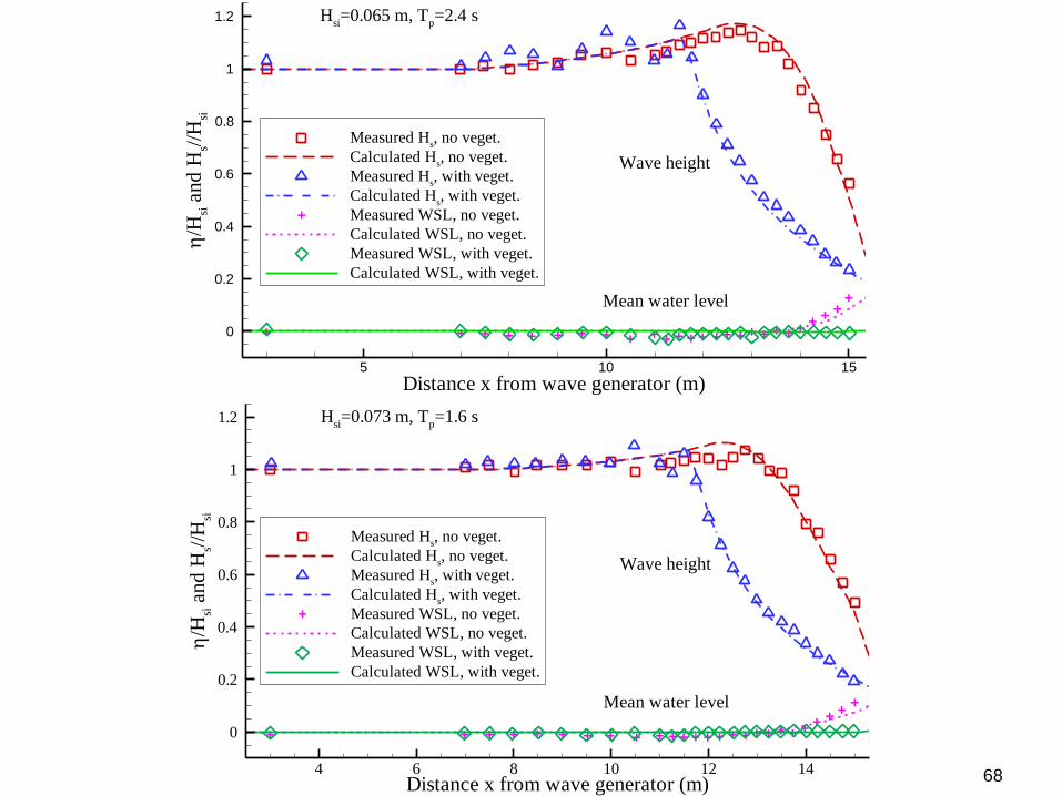
Random Waves through Vegetated Flume

Experiment by Dubi and Torum (1997)

Distance from seaside (m)

Hrm

s(m

)

0 1 2 3 4 5 6 7 8 9 100.06

0.08

0.1

0.12 Measured

Calculated

(a)

Hrms

= 0.114 mT

p= 1.58 s

h = 0.6 mC

D= 0.3

Distance from seaside (m)

Hrm

s(m

)

0 1 2 3 4 5 6 7 8 9 100.06

0.08

0.1

0.12

0.14

Measured

Calculated

(b)

Hrms

= 0.131 mT

p= 2.21 s

h = 0.6 mC

D= 0.18

66

Side View of Wave Runup

67

+ + + + + + + + + + + + + + ++ + + + + + + + + ++

Distance x from wave generator (m)

/H

siand

Hs//H

si

5 10 15

0

0.2

0.4

0.6

0.8

1

1.2

Measured Hs, no veget.

Calculated Hs, no veget.

Measured Hs, with veget.

Calculated Hs, with veget.

Measured WSL, no veget.

Calculated WSL, no veget.

Measured WSL, with veget.

Calculated WSL, with veget.

+

Hsi=0.065 m, T

p=2.4 s

Wave height

Mean water level

+ + + + + + + + + + + + + + + + + + + + + + + + ++

Distance x from wave generator (m)

/H

sian

dH

s//H

si

4 6 8 10 12 14

0

0.2

0.4

0.6

0.8

1

1.2

Measured Hs, no veget.

Calculated Hs, no veget.

Measured Hs, with veget.

Calculated Hs, with veget.

Measured WSL, no veget.

Calculated WSL, no veget.

Measured WSL, with veget.

Calculated WSL, with veget.

+

Hsi=0.073 m, T

p=1.6 s

Wave height

Mean water level

68

Summary

• Effects of vegetation have been extensively investigated by

field and lab experiments and numerical modeling.

• A large set of data have been collected and used to analyze the

vegetation drag coefficient and wave energy dissipation.

• A series of numerical models have been developed to quantify

the wave and surge reduction.

• The models have been tested using a number of laboratory

experiments.

• The drag and inertia forces of vegetation are included in the

2D/3D momentum equations and the wave energy loss due to

vegetation resistance is in the wave-action balance equation.

• The interaction between currents and waves is considered

through a correction factor in the wave dissipation rate.

69

W. Wu, Y. Ozeren, D. Wren, Q. Chen, G. Zhang, M. Holland, Y. Ding, S.N. Kuiry, M. Zhang, R.

Jadhav, J. Chatagnier, Y. Chen, and L. Gordji (2011). Investigation of surge and wave reduction by

vegetation, Phase I Report for SERRI Project No. 80037, The University of Mississippi, MS, p. 315,

with p. 465 Appendices.

W. Wu, Y. Ozeren, D. Wren, Q. Chen, G. Zhang, M. Holland, R. Marsooli, Q. Lin, R. Jadhav, K.R.

Parker, H. Pant, J. Bouanchaud, and Y. Chen (2012). Investigation of surge and wave reduction by

vegetation (Phase II) —Interaction of Hydrodynamics, Vegetation and Soil, Phase II Report for SERRI

Project No. 80037, The University of Mississippi, MS, p. 395.

W. Wu and R. Marsooli (2012). “A depth-averaged 2-D shallow water model for breaking and non-

breaking long waves affected by rigid vegetation.” Journal of Hydraulic Research, IAHR, 50(6), 558–

575.

W. Wu, M. Zhang, Y. Ozeren, and D. Wren (2013). “Analysis of vegetation effect on waves using a

vertical 2-D RANS model.” Journal of Coastal Research, 29(2), 383–397.

W. Wu (2014). “A 3-D phase-averaged model for shallow water flow with waves in vegetated water.”

Ocean Dynamics, 64(7), 1061-1071.

R. Marsooli and W. Wu (2014). “Numerical investigation of wave attenuation by vegetation using a

3D RANS model.” Advances in Water Resources, Accepted for publication.

Y. Ozeren, D. Wren, and W. Wu (2014). “Experimental investigation of wave attenuation through

model and live vegetation.” Journal of Waterway, Port, Coastal, and Ocean Engineering (ASCE),

published online, DOI: 10.1061/(ASCE)WW.1943-5460.0000251.

70

Publications Related