research papers

IUCrJ (2018). 5, 673–680 https://doi.org/10.1107/S2052252518010837 673

IUCrJISSN 2052-2525

PHYSICSjFELS

Received 29 March 2018

Accepted 26 July 2018

Edited by E. E. Lattman, University at Buffalo,

USA

‡ These authors contributed equally to this

work.

Keywords: Rayleigh scattering; XFELs; aerosol

injection; Uppsala injectors; nanoparticles.

Supporting information: this article has

supporting information at www.iucrj.org

Rayleigh-scattering microscopy for tracking andsizing nanoparticles in focused aerosol beams

Max F. Hantke,a,b‡ Johan Bielecki,b,c‡ Olena Kulyk,d Daniel Westphal,b

Daniel S. D. Larsson,b Martin Svenda,b Hemanth K. N. Reddy,b Richard A. Kirian,e

Jakob Andreasson,b,d,f Janos Hajdub,d and Filipe R. N. C. Maiab,g*

aChemistry Research Laboratory, Department of Chemistry, Oxford University, 12 Mansfield Rd, Oxford OX1 3TA, UK,bLaboratory of Molecular Biophysics, Department of Cell and Molecular Biology, Uppsala University, Husargatan 3 (Box

596), Uppsala SE-75124, Sweden, cEuropean XFEL GmbH, Holzkoppel 4, Schenefeld 22869, Germany, dInstitute of

Physics, ELI Beamlines, Academy of Sciences of the Czech Republic, Na Slovance 2, Prague CZ-18221, Czech Republic,eDepartment of Physics, Arizona State University, 550 E. Tyler Drive, Tempe, AZ 85287, USA, fCondensed Matter

Physics, Department of Physics, Chalmers University of Technology, Gothenburg, Sweden, and gNERSC, Lawrence

Berkeley National Laboratory, Berkeley, California, USA. *Correspondence e-mail: filipe@xray.bmc.uu.se

Ultra-bright femtosecond X-ray pulses generated by X-ray free-electron lasers

(XFELs) can be used to image high-resolution structures without the need for

crystallization. For this approach, aerosol injection has been a successful method

to deliver 70–2000 nm particles into the XFEL beam efficiently and at low noise.

Improving the technique of aerosol sample delivery and extending it to single

proteins necessitates quantitative aerosol diagnostics. Here a lab-based

technique is introduced for Rayleigh-scattering microscopy allowing us to track

and size aerosolized particles down to 40 nm in diameter as they exit the

injector. This technique was used to characterize the ‘Uppsala injector’, which is

a pioneering and frequently used aerosol sample injector for XFEL single-

particle imaging. The particle-beam focus, particle velocities, particle density

and injection yield were measured at different operating conditions. It is also

shown how high particle densities and good injection yields can be reached for

large particles (100–500 nm). It is found that with decreasing particle size,

particle densities and injection yields deteriorate, indicating the need for

different injection strategies to extend XFEL imaging to smaller targets, such as

single proteins. This work demonstrates the power of Rayleigh-scattering

microscopy for studying focused aerosol beams quantitatively. It lays the

foundation for lab-based injector development and online injection diagnostics

for XFEL research. In the future, the technique may also find application in

other fields that employ focused aerosol beams, such as mass spectrometry,

particle deposition, fuel injection and three-dimensional printing techniques.

1. Introduction

Extremely intense and short X-ray free-electron laser (XFEL)

pulses can outrun processes of radiation damage (Neutze et al.,

2000) and the short pulse duration permits, in principle,

solving structures at room temperature without the require-

ment for crystallization (Seibert et al., 2011). XFEL single-

particle imaging has been demonstrated on relatively large

samples (70–2000 nm) to moderate resolutions (Seibert et al.,

2011; Hantke et al., 2014; Ekeberg et al., 2015). With continued

improvements to sample delivery techniques, XFEL beam

intensity, beamlines, detectors and reconstruction algorithms,

the XFEL single-particle imaging technique has the potential

to generate structures at high acquisition rates (Hantke et al.,

2014) with particle sizes ranging from several microns (for

example, entire cells) (Bergh et al., 2008) to a few nanometres

(for example, single proteins) (Neutze et al., 2000). In addition,

new strategies have been proposed that make use of inelastic

photoemission and would allow chemically selective imaging

at atomic resolution (Classen et al., 2017).

Despite the extremely bright illumination attainable with

today’s most powerful XFELs, a small particle, such as a

single protein, only gives rise to a faint and noisy diffraction

pattern (Neutze et al., 2000). Signal averaging over many

identical particles is needed to reconstruct the high-resolution

structure.

Efficient sample delivery with low background noise is

central to the success of the approach. Substrate-based sample

delivery for XFEL single-particle imaging of biological

samples has been demonstrated (Seibert et al., 2010; Kimura et

al., 2014) but the presence of a sample container or substrate is

a source of background noise that must be avoided when

aiming for atomic resolution. Atomically thin substrates such

as graphene could potentially solve this problem. Never-

theless, contact to any substrate typically affects structure and

orientation of the deposited sample (Zeng et al., 2017).

Moreover, sample exchanges within less than a microsecond

are required to take full advantage of the rapid repetition

rates of modern XFELs, and this seems unfeasible with

substrate-based techniques and could be challenging with

liquid jets (Stan et al., 2016). Aerosol sample delivery lifts the

requirement for any sample support, which significantly

reduces background scattering and allows for data collection

at high rates (Bogan et al., 2008; Seibert et al., 2011; Hantke et

al., 2014). While aerosol sample delivery is in principle an

elegant approach with attractive advantages, it requires an

aerosol injector that reaches high particle densities for

achieving high hit ratios (i.e. fractions of XFEL pulses that hit

at least one particle) and sufficient particle speed to prevent

multiple exposures.

A pioneering aerosol injector for XFEL single-particle

imaging, the ‘Uppsala injector’ (Seibert et al., 2011; Hantke et

al., 2014) (Fig. 1a), has demonstrated success in numerous

experiments (Seibert et al., 2011; Rath et al., 2014; Hantke et

al., 2014; van der Schot et al., 2015; Ekeberg et al., 2015; Reddy

et al., 2017) for particles between 70 and 2000 nm in diameter.

The injector is available for users at the Linac Coherent Light

Source (LCLS), the European XFEL, the Free Electron laser

Radiation for Multidisciplinary Investigations (FERMI) and

the Extreme Light Infrastructure (ELI) Beamlines facility.

Despite its successful and frequent use, the particle-beam

properties as a function of operating conditions that are

relevant for XFEL single-particle imaging have not yet been

extensively characterized and described in the literature.

Traditionally, focused-aerosol-particle beams have been

examined on the basis of dusting spots (Murphy & Sears, 1964;

Williams et al., 2013) or, in the case of charged aerosols, using

ion detectors (Schreiner et al., 1999; Williams et al., 2013).

Recently, visualization of relatively large (down to 200 nm)

aerosol-injected particles has been demonstrated (Kirian et al.,

2015; Awel et al., 2016, 2018). Here we describe a Rayleigh-

scattering-microscopy setup (Fig. 1b) that extends the size

range of this approach down to 40 nm in diameter and that can

be used to directly measure positions, velocity and, as an

additional quantity, the diameter of single aerosol particles.

We used our Rayleigh-microscopy setup to characterize the

particle-beam properties of the Uppsala injector. We present

results on particle focusing, velocity, particle density and

overall injection yield as functions of operating conditions. We

discuss implications of our results for XFEL single-particle

imaging and strategies for future injector development.

2. Results

2.1. Experimental setup

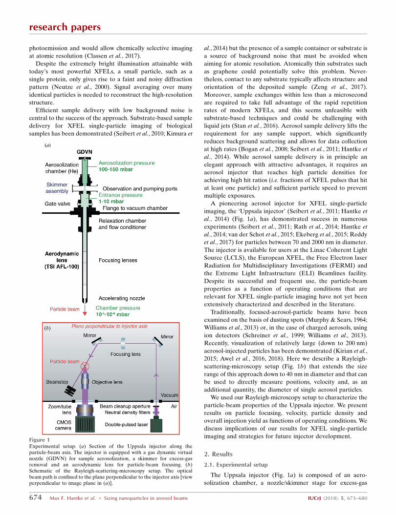
The Uppsala injector (Fig. 1a) is composed of an aero-

solization chamber, a nozzle/skimmer stage for excess-gas

research papers

674 Max F. Hantke et al. � Sizing nanoparticles in areosol beams IUCrJ (2018). 5, 673–680

Figure 1Experimental setup. (a) Section of the Uppsala injector along theparticle-beam axis. The injector is equipped with a gas dynamic virtualnozzle (GDVN) for sample aerosolization, a skimmer for excess-gasremoval and an aerodynamic lens for particle-beam focusing. (b)Schematic of the Rayleigh-scattering-microscopy setup. The opticalbeam path is confined to the plane perpendicular to the injector axis [viewperpendicular to image plane in (a)].

removal (Campargue, 1984; Beijerinck et al., 1985) and an

aerodynamic lens (Murphy & Sears, 1964; Bogan et al., 2008;

Liu et al., 1995a,b) for aerosol focusing at the XFEL beam

focus [usually 0.1 to several tens of microns in diameter

(Boutet & Williams, 2010; Bostedt et al., 2013; Feldhaus,

2010)]. The pressure decreases gradually as the particle-laden

gas flows through the injector compartments. In the first

compartment the sample solution is aerosolized with a gas

dynamic virtual nozzle (GDVN) (Ganan-Calvo, 1998;

DePonte et al., 2008) in a 100–250 mbar He atmosphere. After

aerosolization, excess gas is skimmed away by differential

pumping in the nozzle-skimmer stage. Downstream of the

skimmer the aerosol particles enter the aerodynamic lens at a

pressure between 0.5 and 3.5 mbar (aerodynamic lens

entrance pressure). Particles exit the aerodynamic lens

through an acceleration tube and a 1.5 mm aperture, and enter

the experimental chamber, which is kept at 10�6–10�4 mbar

(vacuum-chamber pressure).

A double-pulsed green laser illuminates particles as they

exit the injector. Images are taken with a microscope equipped

with a CMOS camera (Fig. 1b). The double-flash illumination

results in two particle images per exposure. Velocities are

determined from the relative distances and the inter-pulse

delay (Fig. 2a). The data are analyzed with our open-source

software package (https://github.com/mhantke/spts), which

determines particle positions, velocities and particle diameters

from the images (Figs. 2a and 2b).

With two laser pulses delayed by 0.5 ms the lateral extent of

the laser-beam spot [i.e. 0.5 mm full width at half-maximum

(FWHM)] permits, in principle, the measurement of velocities

up to 1000 ms�1. The injector points downwards into the

experimental chamber while the path of the laser beam and

the optical axis of the microscope are confined to the hori-

zontal plane. The optical axis of the microscope intersects the

laser-beam axis at an angle of 25�. Generally, the Mie-

scattering law can be used to estimate the particle brightness

as a function of particle diameter (Bohren & Huffman, 1983).

In this small-angle scattering configuration the particles with

diameters up to 200 nm can be considered as Rayleigh scat-

terers and the scattering intensity is proportional to the sixth

power of the particle diameter. We confirmed this scaling law

for our setup by measuring the particle brightness in images of

polystyrene-sphere size standards (Fig. 2c). The Rayleigh-

scattering intensity increases monotonically with particle

diameter. This means that, if suitable calibration data (as

shown in Fig. 2c) are available, diameters of particles of

unknown size may be determined from the measured particle

brightness in the image. For a 40 nm polystyrene sphere we

measured an average scattering intensity of 157 photons per

50 mJ pulse with an optical system of 0.055 numerical aper-

ture. Attempts at imaging even smaller 20 nm sized injected

polystyrene spheres failed at this pulse energy. This was

expected as their scattering signal is 64 times lower than for

the 40 nm spheres (three photons per particle), not exceeding

average background fluctuations (four photons per pixel).

Particles larger than 125 nm could not be quantitatively sized

because of the limited linear dynamic range of the detector.

These are technical limitations, which could be overcome by a

tighter laser focus, higher pulse energies, a larger numerical

aperture for the objective lens and a higher dynamic range for

the detector.

2.2. Particle-beam focusing

To study the particle-beam evolution as a function of

particle diameter and entrance pressure of the aerodynamic

lens we recorded separate data sets for polystyrene spheres

with mean diameters between 40 and 495 nm. Data were

collected for about 1.5 min at a frame rate of 15 Hz resulting in

about 1000 images per data set. We observed one to 30

particles per frame depending on particle size, particle

concentration, injector pressure and distance from the exit

orifice of the aerodynamic lens. The field of view was confined

to the illumination spot. To examine the particle-beam

research papers

IUCrJ (2018). 5, 673–680 Max F. Hantke et al. � Sizing nanoparticles in areosol beams 675

Figure 2Quantitative analysis of Rayleigh-scattering-microscopy data. (a)Double-exposure image of two polystyrene spheres of differentdiameters. The pulse delay was 50.8 ms and the pulse energy 56.1 mJ.(b) Extracted particle positions, velocities and diameters from the imageshown in (a). (c) The sixth root of the mean integrated scattering intensityper particle (rescaled to 1 mJ laser-pulse energy) is plotted against thediameter of the respective polystyrene-sphere size standard. The valuesfollow Rayleigh’s scattering law (solid line).

evolution, we translated the injector along the particle-beam

axis and measured recorded data for a range of entrance

pressures, particle diameters and distances from the injector

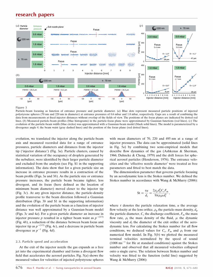
tip (‘injector distance’) (Fig. 3a). Particle clusters, caused by

statistical variation of the occupancy of droplets generated by

the nebulizer, were identified by their larger particle diameter

and excluded from the analysis (see Fig. S1 in the supporting

information). The data show that for a given particle size an

increase in entrance pressure results in a contraction of the

beam profile (Figs. 3a and 3b). As the particle size or entrance

pressure increases, the particle beam became tighter, less

divergent, and its focus (here defined as the location of

minimum beam diameter) moved closer to the injector tip

(Fig. 3c). At any given injector distance, the particle-density

profile transverse to the beam direction followed a Gaussian

distribution (Figs. 3b and S1 in the supporting information)

and the evolution of the particle beam as a function of injector

distance was well approximated by a Gaussian-beam model

(Figs. 3c and 4a). For a given particle diameter an increase in

injector pressure p resulted in a tighter beam waist as p�(2/3)

(Fig. 4b), a reduction of the distance between beam focus and

injector tip as p�(1/2) (Fig. 4c), and a decrease in particle beam

divergence as p�1 (Fig. 4d).

2.3. Particle speed and acceleration

At the exit of the injector nozzle the gas expands as a free

jet into the experimental chamber and forms a divergent flow

field that accelerates the aerosol particles. Fig. 5(a) shows the

measured values for velocities of injected polystyrene spheres

with mean diameters of 70, 220 and 495 nm at a range of

injector pressures. The data can be approximated (solid lines

in Fig. 5a) by combining two semi-empirical models that

describe flow dynamics of the gas (Ashkenas & Sherman,

1966; Dahneke & Cheng, 1979) and the drift forces for sphe-

rical aerosol particles (Henderson, 1976). The entrance velo-

cities and the ‘effective nozzle diameter’ were treated as free

parameters and fitted to best match the data.

The dimensionless parameter that governs particle focusing

by an aerodynamic lens is the Stokes number. We defined the

Stokes number in accordance with Wang & McMurry (2006):

St ¼�u

df

¼2�pd2

pCcFm

9��l�d3f

;

where � denotes the particle relaxation time, u the average

flow velocity at the lens orifice, �p the particle-mass density, dp

the particle diameter, Cc the discharge coefficient, Fm the mass

flow rate, �l the mass density of the fluid, � the dynamic

viscosity and df the diameter of the exit orifice of the aero-

dynamic lens. For calculating the Stokes number for all flow

conditions, we deduced values for Cc, Fm and �l from our

numerical flow model. In Fig. 5(b) we plotted the measured

terminal velocities normalized by the speed of sound

(1008 ms�1 for He at standard conditions) against the Stokes

number and observed that all measured velocities collapsed

onto a single curve. The relation between Stokes number and

velocity was fitted to the function (solid line) suggested by

Wang & McMurry (2006):

research papers

676 Max F. Hantke et al. � Sizing nanoparticles in areosol beams IUCrJ (2018). 5, 673–680

Figure 3Particle-beam focusing as function of entrance pressure and particle diameter. (a) Blue dots represent measured particle positions of injectedpolystyrene spheres (70 nm and 220 nm in diameter) at entrance pressures of 0.6 mbar and 1.8 mbar, respectively. Gaps are a result of combining thedata from measurements at fixed injector distances without overlap of the fields of view. The positions of the focus planes are indicated by dotted redlines. (b) Measured particle-beam profiles (blue histograms) in the particle-focus plane were approximated by Gaussian functions (red lines). (c) Theevolution of the particle-beam width (blue circles) was approximated with a Gaussian-beam model (black solid lines). The model is parameterized by adivergence angle �, the beam waist (gray dashed lines) and the position of the focus plane (red dotted lines).

v1c¼ðAþ B StÞ

ð1þ C StÞ:

We obtain the best fit to our data for A = 0.486, B = 0.002 and

C = 0.088, which roughly match data that Wang & McMurry

(2006) reported for Stokes numbers below 100 (Fig. 5b). Our

data extends to higher Stokes numbers for which, to our

knowledge, no data has been published that we could use for

comparative purposes.

2.4. Particle densities

We determined the particle density as a function of particle

diameter and entrance pressure (Fig. 6a) at a flow rate of

1 ml min�1 and a concentration of 1012 particles per ml. We

found that for a given particle size between 40 and 495 nm the

maximum areal particle-number density was in the range of

4 � 10�4 to 1.9 � 10�2 particles per mm2 (Fig. 6a). By

comparing the inflow of particles (particle concentration �

sample flow rate) to the outflow from the injector (particle-

number density � cross-sectional beam area � particle velo-

city) we determined the maximum particle-injection yield,

from solution into vacuum, as 22 and 45% depending on

particle diameter (Fig. 6b).

Particles accelerate after they pass the last orifice and

therefore the location of maximum particle density does not

necessarily coincide with the focus position (i.e. the location of

minimum beam diameter). We determined the areal particle-

number density as a function of injector distance (see Fig. S2

in the supporting information) and found that the location of

its maximum matches the position of the focus to the precision

of our measurements.

3. Discussion

In this work we introduced a lab-based technique that allows

tracking and sizing of unlabeled aerosol particles as they are

injected into a vacuum chamber. We applied this technique to

characterize the Uppsala injector, which has been the

pioneering sample injector for XFEL imaging. Our data

enabled us to determine particle-beam characteristics as a

function of particle diameter and aerodynamic lens entrance

pressure.

research papers

IUCrJ (2018). 5, 673–680 Max F. Hantke et al. � Sizing nanoparticles in areosol beams 677

Figure 4Scaling laws for the particle-beam focus with respect to entrance pressure.(a) Particle-beam widths (FWHM) for a range of pressures (see legend)are plotted against the distance from the injector tip. Particles werepolystyrene spheres of 100 nm in diameter. The experimental data can beapproximated with a Gaussian-beam model (solid lines). Scaling laws[solid lines in (b), (c) and (d)] were identified for the model parameters asfunctions of the entrance pressure p. (b) The particle-beam waist scales asp�(3/2). (c) The distance between particle focus and injector tip scales asp�(1/2). (d) The particle-beam divergence scales as p�1.

Figure 5Particle speed and acceleration. (a) Particle velocity as a function of theirdistance from the exit orifice of the injector for polystyrene spheres of 70,220 and 495 nm in diameter at pressures between 0.6 and 1.8 mbar. Thesolid lines show the approximated velocity evolution according to ourmodel. (b) Terminal-velocity values normalized to the speed of soundplotted against the Stokes number. We compare our data (filled circles) tosimulated and experimental data reported by Wang & McMurry (2006)for the same lens system with air as a carrier gas and at higher injectorpressures than studied here.

3.1. Characterization of the aerodynamic lens

We found that the particle-beam profile of the Uppsala

injector is represented accurately by a Gaussian-beam model

for the range of tested conditions (40–500 nm particle

diameter, 0.5–2.0 mbar entrance pressure). An increase in

entrance pressure and particle diameter results in a contrac-

tion of the beam profile. For a fixed particle diameter, the

contraction is characterized by a tighter beam waist, shorter

focus distance and lower particle-beam divergence, each

governed by a simple scaling law of the entrance pressure.

We developed a numerical model to describe the accel-

eration of particles as they exit the aerodynamic lens. The

model allowed us to assign a Stokes number to each

measurement. Data points of final particle velocity plotted

against the Stokes number collapse onto a single curve. The

curve is in agreement with previous results (Wang & McMurry,

2006) and extends beyond. Our velocity measurements show

that even the largest particles (500 nm) are fast enough

(>20 m s�1) to pass through a 1 mm focus within the time gap

between two X-ray pulses given the 4.4 MHz repetition rate of

the European XFEL. This means that the particles are fast

enough to clear the interaction volume between subsequent

pulses. This permits, in principle, data collection at the theo-

retical maximum rate (Hantke et al., 2014).

3.2. Particle size

We showed that the brightness of single particles in our

images follows the Rayleigh-scattering law. We demonstrated

that, with a calibration curve, injected particles between 40

and 125 nm in diameter can not only be detected but also

sized. This is particularly useful for XFEL single-particle

imaging because the undesired presence of non-volatile

contaminants or insufficient particle desolvation can be

discovered by a mismatch in the size distributions of sample

particles before and after aerosolization (Kassemeyer et al.,

2012; Daurer et al., 2017). The ability to test in the lab injection

of any given sample helps to identify suitable sample buffers

and sample concentrations prior to data collection at XFELs.

This information is essential for optimizing sample injection

for XFEL single-particle imaging and difficult to obtain by

other means.

3.3. Particle densities

We showed that the particle densities that can be reached

with the Uppsala injector depend significantly on particle

diameter and entrance pressure. For the studied range of

conditions, we found that particle densities increase with

particle diameter and entrance pressure. We measured areal

particle densities of up to 4 � 10�4 to 1.9 � 10�2 particles per

mm2 depending on particle diameter. The effective area of the

focus is the region of the focus that is intense enough to

produce measurable diffraction from a single particle. If we

assumed that the nominal focus area [i.e. �(FWHM/2)2]

matched the area of the focus region that is intense enough for

producing measurable diffraction from a single particle, we

would predict lower hit ratios (0.0003–37% for FWHM of

0.1–5 mm) than those that were in fact reached (between

0.8–79%) during past XFEL single-particle imaging experi-

ments (Hantke et al., 2014; Schot et al., 2015; Reddy et al., 2017;

Daurer et al., 2017). In fact, the effective focus area depends

on many, mostly poorly known, variables, such as the intensity

distribution in the interaction region, the beamline

background, the detector response and the particle’s structure

and orientation. For two XFEL single-particle imaging data

sets (Hantke et al., 2014; Daurer et al., 2017) distributions of

X-ray beam intensities of hits were determined from the

diffraction data. In both cases the data showed that most

diffraction patterns originated from weak hits at X-ray

intensities far below half-maximum beam intensity (Hantke et

al., 2014; Daurer et al., 2017). This means that for those

experiments the effective focus area was considerably larger

than the nominal focus area. We would expect the opposite for

data acquired on much smaller particles under the same

conditions.

For very high hit ratios the superposition of strong and

spurious hits in a single diffraction pattern may present a

problem (Hantke et al., 2014). Therefore, moderate hit ratios

(10–20%), as have been reached with the Uppsala injector for

relatively large particles (100–500 nm), seem presently

acceptable. Yet, the drastically lower particle densities for

smaller particles, such as proteins, call for dedicated injector

development.

Our results suggest that one possible strategy for reaching

higher particle densities would be to increase the aerodynamic

lens entrance pressure. But high aerodynamic lens entrance

pressures are typically associated with high gas load on the

sample chamber and interfere with vacuum requirements for

research papers

678 Max F. Hantke et al. � Sizing nanoparticles in areosol beams IUCrJ (2018). 5, 673–680

Figure 6Particle density (a) and overall particle-injection yield (b) as a function ofaerodynamic lens entrance pressure for polystyrene spheres with a rangeof distinct diameters (see legends). For (a) we normalized the values tothe conditions of a particle solution with a concentration of 1012 particlesper ml and a flow rate of 1 ml min�1.

X-ray detectors and other beamline equipment. In addition,

high gas pressures in the focus can also cause undesired X-ray

background noise. These problems could be mitigated to some

extent by incorporating a differentially pumped shroud

around the injector.

4. Conclusion

Our results demonstrate the power of Rayleigh-scattering

microscopy for tracking and sizing of focused aerosol particles.

We anticipate that our characterization of the Uppsala injector

will be useful to optimize data rates and data quality in future

XFEL single-particle imaging experiments and will guide the

development of new injectors in particular for small particles.

New injection strategies are needed for reaching high particle

densities, also for small particles, and unlocking the potential

of femtosecond imaging on single molecules and chemical

complexes. Furthermore, we envision that our Rayleigh-scat-

tering-microscopy method will find application in other fields

that employ focused aerosol beams, such as mass spectro-

metry, particle deposition and three-dimensional printing

techniques.

5. Methods

5.1. Experimental setup

The stream of injected particles exiting from the tip of the

aerodynamic lens was intersected with the single/dual-pulsed

frequency-doubled Nd:YAG laser (Quantel Evergreen 25100,

532 nm wavelength). The laser provided pulse energies of up

to 117 mJ resulting in peak intensities of 149 mJ mm2 at 7 ns

pulse duration. The laser beam was focused by a plano-convex

lens with 20 cm focal length to 0.6 mm FWHM at the inter-

section point with the particle beam. The laser beam was

coupled into the experimental chamber through a glass

window and was redirected three times by three consecutive

mirrors, two before and one after the interaction point. Stray

light was reduced by coupling the laser after the final mirror

into a conical beam dump. For every measurement, the

selection of pulse energy and neutral density absorption filter

were optimized in order to obtain maximal signal while

avoiding overexposure of the camera.

Particles were imaged with a microscope that is comprised

of a stationary 2� objective lens (NA = 0.055, 91 mm depth of

focus), placed inside the experimental chamber, and a

motorized zoom lens (Navitar 12� UltraZoom) and CMOS

camera (Hamamatsu Orca-Flash4.0 V2) on the outside. The

optical axis of the microscope was aligned vertically with

respect to the particle beam such that the angle between its

optical axis and the laser-beam axis measured 25�.

The camera had 2048 � 2048 pixels, each with a sensitive

area of 6.5 � 6.5 mm. The quantum efficiency was 0.8 and

pixels were saturated at a signal of about 30 700 photons. The

camera was operated at room temperature. Frames were

acquired at a rate of 15 Hz in synchronization with the laser

pulses. From 500 exposures we measured a mean photon

background of 0.12 photons per pixel and per mJ of pulse

energy at dark-noise fluctuations of, on average, 1.3 photons

per pixel. The positional resolution in the image plane of

1.14 mm was calculated on the basis of the camera’s pixel

spacing and the microscope lens’ configuration.

5.2. Image processing

From the camera frames, peaks were detected and analyzed

in a data analysis pipeline (https://github.com/mhantke/spts).

For peak picking, two differently blurred versions of the image

were generated using Gaussian kernels. The blur parameter �was 0.03 and 0.06 pixels for the two versions. The difference

image of the two blurred images was thresholded and a peak

was assigned to each isolated cluster of pixels with values

above a manually set threshold. For every measurement the

threshold was adjusted manually to a value well above back-

ground fluctuations to minimize the selection of spurious

peaks. From each peak, the particle position was determined

by calculating the center of mass of the selected pixels. Back

reflection resulted in the appearance of an additional faint

peak at a constant displacement with respect to the main peak.

We identified these spurious peaks and excluded them from

further analysis. The brightness of each peak was determined

by integrating the measured pixel values up to a radial

distance of 10 pixels from the peak position. Peaks that were

closer than 21 pixels apart were excluded from any further

analysis.

5.3. Intensity calibration

We injected suspensions of monodisperse polystyrene

sphere size standards (Fischer Scientific, NIST-traceable size

standard) to establish the relationship of peak brightness to

particle diameter. The diameters of the size standards were

41 � 4, 60 � 4, 70 � 3, 81 � 3, 100 � 3 and 120 � 3 nm, and

their variation coefficients were n.a., 17, 10.4, 11.7, 7.8 and

3.6%, respectively. The brightness of each particle was

rescaled to its illumination using the beam profile, which we

measured with a screen in a separate measurement. Calibra-

tion results are shown in Fig. 2(c) and are in agreement with

the power law for Rayleigh scattering.

5.4. Model for particle acceleration

Particle acceleration was modeled by calculating the drag of

spherical particles in a freely expanding jet. The flow through

the exit orifice (1.5 mm in diameter) forms a laminar

(Re ’ 1–100) continuous (Kn ’ 10�2–10�1) flow field.

Aerosol particles (40–500 nm in diameter) are about four

orders of magnitude smaller than the orifice. Therefore, the

Knudsen number for particle drag is about four orders of

magnitude larger (Kn ’ 102–103) and the flow field that is

responsible for particle drag is governed by the laws of free

molecular flow. We used the formula that estimates the spatial

evolution of the Mach number at the centerline of a free jet

(Ashkenas & Sherman, 1966; Dahneke & Cheng, 1979) to

estimate the gas-flow field. The drag force was computed using

a semi-empirical formula (Henderson, 1976), which is accurate

research papers

IUCrJ (2018). 5, 673–680 Max F. Hantke et al. � Sizing nanoparticles in areosol beams 679

for spherical particles at free-molecular-flow conditions. Gas

velocity and the local state parameters of gas pressure, density

and temperature were derived from the Mach number.

Particles were inserted in the model system at a given initial

velocity and propagated in the one-dimensional gas flow in an

iterative scheme with dynamic adjustment of the step size to

ensure accurate results while keeping computation time low.

For the ratio of effective and physical orifice diameter the

best fit suggested a value of 0.880. Ashkenas & Sherman

(1966) measured a value of 0.943 for a thin-plate orifice of

similar dimensions to ours at nozzle Reynolds numbers above

500. The Reynolds numbers relevant for the study here are

lower (Re ’ 1–100). As the boundary layer at the orifice

increases with decreasing Reynolds number the relatively

smaller effective orifice diameter that we obtain is expected.

5.5. Sample preparation and aerosolization

NIST-traceable polystyrene calibration spheres with

diameters between 40 and 500 nm in an aqueous solution of

1011 particles ml�1 were used for the measurements. The

nanospheres were aerosolized from the jet breakup of a

1.5 mm liquid jet from a GDVN running with 1–2 ml min�1 flow

rate. With these conditions, between two to five particles were

observed per frame on the camera, depending on particle

diameter and injector pressure.

Acknowledgements

J. Bielecki and M. F. Hantke designed the Rayleigh-scattering-

microscopy setup with input from F. R. N. C. Maia, and R.

Kirian, D. S. D. Larsson and O. Kulyk manufactured nozzles

for sample aerosolization. H. K. N. Reddy, J. Bielecki and

O. Kulyk prepared the samples. D. Westphal, J. Hajdu,

J. Andreasson and M. Svenda developed the injector.

J. Bielecki, M. F. Hantke and O. Kulyk carried out the

measurements. M. F. Hantke and J. Bielecki analysed the data.

M. F. Hantke wrote the analysis software and carried out the

numerical simulation. M. F. Hantke and J. Bielecki wrote the

manuscript with input from F. R. N. C. Maia, J. Hajdu,

D. S. D. Larsson and R. Kirian. All authors approved of the

final manuscript.

Funding information

This work was supported by the Wellcome Trust (204732/Z/16/

Z), the Swedish Research Council, the Swedish Foundation

for Strategic Research, the Rontgen-Angstrom Cluster, the

projects Advanced research using high intensity laser

produced photons and particles (ADONIS) (CZ.02.1.01/0.0/

0.0/16_019/0000789) and Structural dynamics of biomolecular

systems (ELIBIO) (CZ.02.1.01/0.0/0.0/15_003/ 0000447) from

the European Regional Development Fund and the NSF STC

Award ‘BioXFEL’ (1231306). J. Andreasson acknowledges

support of the Ministry of Education, Youth and Sports as part

of targeted support from the National Programme of

Sustainability II and the Chalmers Area of Advance; Mate-

rials Science. The contribution of O. Kulyk is part of a project

that has received funding from the European Union’s Horizon

2020 research and innovation programme under grant agree-

ment No. 654220. The authors declare no competing financial

interests.

References

Ashkenas, H. & Sherman, F. S. (1966). Rarefied Gas Dynamics, Vol. 2,edited by J. H. De Leeuw, pp. 84–105. New York: Academic Press.

Awel, S., Kirian, R. A., Eckerskorn, N., Wiedorn, M., Horke, D. A.,Rode, A. V., Kupper, J. & Chapman, H. N. (2016). Opt. Express, 24,6507–6521.

Awel, S. et al. (2018). J. Appl. Cryst. 51, 133–139.Beijerinck, H. C. W., Van Gerwen, R. J. F., Kerstel, E. R. T., Martens,

J. F. M., Van Vliembergen, E. J. W., Smits, M. r. Th. & Kaashoek, G.H. (1985). Chem. Phys. 96, 153–173.

Bergh, M., Huldt, G., Tımneanu, N., Maia, F. R. N. C. & Hajdu, J.(2008). Q. Rev. Biophys. 41, 181–204.

Bogan, M. J. et al. (2008). Nano Lett. 8, 310–316.Bohren, C. F. & Huffman, D. R. (1983). Absorption and Scattering of

Light by Small Particles. New York: WileyBostedt, C. et al. (2013). J. Phys. B At. Mol. Opt. Phys. 46, 164003.Boutet, S. & Williams, G. J. (2010). New J. Phys. 12, 035024.Campargue, R. (1984). J. Phys. Chem. 88, 4466–4474.Classen, A., Ayyer, K., Chapman, H. N., Rohlsberger, R. & von

Zanthier, J. (2017). Phys. Rev. Lett. 119, 053401.Dahneke, B. E. & Cheng, Y. S. (1979). J. Aerosol Sci. 10, 257–274.Daurer, B. J. et al. (2017). IUCrJ, 4, 251–262.DePonte, D. P., Weierstall, U., Schmidt, K., Warner, J., Starodub, D.,

Spence, J. C. H. & Doak, R. B. (2008). J. Phys. D Appl. Phys. 41,195505.

Ekeberg, T. et al. (2015). Phys. Rev. Lett. 114, 1–6.Feldhaus, J. (2010). J. Phys. B At. Mol. Opt. Phys. 43, 194002.Ganan-Calvo, A. (1998). Phys. Rev. Lett. 80, 285–288.Hantke, M. F. et al. (2014). Nat. Photon. 8, 943–949.Henderson, C. B. (1976). AIAA J. 14, 707–708.Kassemeyer, S. et al. (2012). Opt. Express, 20, 4149–4158.Kimura, T., Joti, Y., Shibuya, A., Song, C., Kim, S., Tono, K., Yabashi,

M., Tamakoshi, M., Moriya, T., Oshima, T., Ishikawa, T., Bessho, Y.& Nishino, Y. (2014). Nat. Commun. 5, 3052.

Kirian, R. A. et al. (2015). Struct. Dyn. 2, 041717.Liu, P., Ziemann, P. J., Kittelson, D. B. & McMurry, P. H. (1995a).

Aerosol Sci. Technol. 22, 293–313.Liu, P., Ziemann, P. J., Kittelson, D. B. & McMurry, P. H. (1995b).

Aerosol Sci. Technol. 22, 314–324.Murphy, W. K. & Sears, G. W. (1964). J. Appl. Phys. 35, 1986–1987.Neutze, R., Wouts, R., van der Spoel, D., Weckert, E. & Hajdu, J.

(2000). Nature, 406, 752–757.Rath, A. D. et al. (2014). Opt. Express, 22, 28914–28925.Reddy, H. K. N. et al. (2017). Sci. Data, 4, 170079.Schot, G. van der et al. (2015). Nat. Commun. 6, 5704.Schreiner, J., Schild, U., Voigt, C. & Mauersberger, K. (1999). Aerosol

Sci. Technol. 31, 373–382.Seibert, M. M. et al. (2010). J. Phys. B At. Mol. Opt. Phys. 43, 194015.Seibert, M. M. et al. (2011). Nature, 470, 78–81.Stan, C. A. et al. (2016). Nat. Phys. 12, 966–971.Wang, X. & McMurry, P. H. (2006). Aerosol Sci. Technol. 40, 320–334.Williams, L. R. et al. (2013). Atmos. Meas. Tech. 6, 3271–3280.Zeng, C., Hernando-Perez, M., Dragnea, B., Ma, X., van der Schoot,

P. & Zandi, R. (2017). Phys. Rev. Lett. 119, 038102.

research papers

680 Max F. Hantke et al. � Sizing nanoparticles in areosol beams IUCrJ (2018). 5, 673–680