research on the mechanics of cfrp composite lap … · research on the mechanics of cfrp composite...
TRANSCRIPT

Research on the Mechanics of CFRP Composite Lap Joints
by
Austin Curnutt
B.S., Kansas State University, 2017
A THESIS
submitted in partial fulfillment of the requirements for the degree
MASTER OF SCIENCE
Department of Architectural Engineering
College of Engineering
KANSAS STATE UNIVERSITY
Manhattan, Kansas
2017
Approved by:
Major Professor
Donald Phillippi, Ph.D., S.E., Architect

Copyright
© AUSTIN CURNUTT
2017
Abstract
For this thesis, research was performed on CFRP bonded composite lap-joints with one
and two continuous laminas through the lap. Composite wraps used to retrofit existing structures
use lap joints to maintain their integrity. The use of composites for retrofitting structures has
many advantages over traditional methods, such as steel jacketing, and is becoming more widely
accepted in the structural engineering industry. While much literature exists documenting the
performance of composite wraps as a whole when applied to concrete columns, less information
is available on the behavior of the lap-joint of the wrap. Developing a better understanding of
how the lap-joint behaves will help researchers further understand composite column wraps. This
research sought to determine what affect continuous middle laminas may have on the stiffness of
lap joints and whether or not stress concentrations exist in the lap-joint due to a change in
stiffness.

iv
Table of Contents
List of Figures ................................................................................................................................ vi
List of Tables ................................................................................................................................. ix
Acknowledgements ......................................................................................................................... x
Symbols List .................................................................................................................................. xi
Chapter 1 - Introduction .................................................................................................................. 1
Chapter 2 - Literature Review ......................................................................................................... 2
2.1. Single-lap Joints ............................................................................................................... 4
2.2. Double-lap Joints ........................................................................................................... 10
Chapter 3 - Experiment ................................................................................................................. 14
3.1 Problem description ........................................................................................................ 14
3.2 Specimen construction .................................................................................................... 15
3.3 Specimen properties ........................................................................................................ 19
3.4 Test set-up ....................................................................................................................... 19
Chapter 4 - Theoretical Models .................................................................................................... 22
4.1 Stiffness equation model ................................................................................................. 22
4.2 Modified Volkersen model ............................................................................................. 24
4.3 Specimen strength ........................................................................................................... 25
Chapter 5 - Results and Conclusion .............................................................................................. 28
5.1 Results ............................................................................................................................. 28
5.1.1 Experimental results................................................................................................. 28
5.1.2 Modified Volkersen model results ........................................................................... 35
5.2 Reasons for error and recommendations for future research .......................................... 37
5.3 Conclusion ...................................................................................................................... 38
References ..................................................................................................................................... 40
Appendix A - Experiment Results ................................................................................................ 42
Specimen 0.2A .................................................................................................................. 42
Specimen 0.3A .................................................................................................................. 44
Specimen 0.4A .................................................................................................................. 45
Specimen 1.3 test results ................................................................................................... 47

v
Specimen 1.4 test results ................................................................................................... 48
Specimen 1.5 test results ................................................................................................... 50
Specimen 1.6 test results ................................................................................................... 51
Specimen 2.1 test results ................................................................................................... 53
Specimen 2.2 test results ................................................................................................... 54
Specimen 2.3 test results ................................................................................................... 56
Appendix B - Modified Volkersen Model Results ....................................................................... 58
Specimen 0.2A .................................................................................................................. 59
Specimen 0.3 A ................................................................................................................. 60
Specimen 0.4A .................................................................................................................. 62
Specimen 1.3 ..................................................................................................................... 63
Specimen 1.4 ..................................................................................................................... 65
Specimen 1.5 ..................................................................................................................... 66
Specimen 1.6 ..................................................................................................................... 68
Specimen 2.1 ..................................................................................................................... 69
Specimen 2.2 ..................................................................................................................... 71
Specimen 2.3 ..................................................................................................................... 72

vi
List of Figures
Figure 1. Single-lap joint geometry ................................................................................................ 4
Figure 2. Single-lap joint with spew fillet ...................................................................................... 5
Figure 3. Failure modes of laminate ............................................................................................... 8
Figure 4. Failure modes of unidirectional lamina in longitudinal tension ...................................... 9
Figure 5. Double-lap joint geometry ............................................................................................. 10
Figure 6. Lap-joint with end mismatch ......................................................................................... 13
Figure 7. Lap-joint with one continuous middle layer .................................................................. 14
Figure 8. Lap-joint with two continuous middle layers ................................................................ 14
Figure 9. Wood block used to form the CFRP wraps ................................................................... 15
Figure 10. Saturating the carbon fibers with neat resin ................................................................ 16
Figure 11. Flipping the block along the table to apply the fabric ................................................. 17
Figure 12. Flipping the block along the table to apply the fabric ................................................. 17
Figure 13. Saw used to cut specimens .......................................................................................... 18
Figure 14. Saw used to cut specimens .......................................................................................... 18
Figure 15. Steel pin used for tensile test ....................................................................................... 20
Figure 16. Set-up showing tube in center ..................................................................................... 21
Figure 17. Test set-up ................................................................................................................... 21
Figure 18. Experimental set-up ..................................................................................................... 22
Figure 19. Free body diagram of CFRP around pin...................................................................... 22
Figure 20. Example of force vs. displacement chart using test data ............................................. 28
Figure 21. Example of strain vs. displacement chart using test data ............................................ 29
Figure 22. Example stress vs. strain curves .................................................................................. 31
Figure 23. Example plot of adhesive shear stress vs. distance from the lap center point ............. 36
Figure 24. Example plot of lap stiffness calculated from modified Volkersen model ................. 36
Figure 25. 0.2A lap test result ....................................................................................................... 42
Figure 26. 0.2A off lap test result ................................................................................................. 43
Figure 27. 0.2A Back side test results........................................................................................... 43
Figure 28. 0.3A Lap test results .................................................................................................... 44
Figure 29. 0.3A off lap test results ................................................................................................ 44

vii
Figure 30. 0.3A Back side test results........................................................................................... 45
Figure 31. 0.4A Lap results ........................................................................................................... 45
Figure 32. 0.4A Off lap test results ............................................................................................... 46
Figure 33. 0.4A Back side test results........................................................................................... 46
Figure 34. 1.3 Lap test results ....................................................................................................... 47
Figure 35. 1.3 Off lap test results .................................................................................................. 47
Figure 36. 1.3 Back side test results ............................................................................................. 48
Figure 37. 1.4 Lap test results ....................................................................................................... 48
Figure 38. 1.4 Off lap test results .................................................................................................. 49
Figure 39. 1.4 Back side test results ............................................................................................. 49
Figure 40. 1.5 Lap test results ....................................................................................................... 50
Figure 41. 1.5 Off lap test results .................................................................................................. 50
Figure 42. 1.5 Back side test results ............................................................................................. 51
Figure 43. 1.6 Lap test results ....................................................................................................... 51
Figure 44. 1.6 Off lap test results .................................................................................................. 52
Figure 45. 1.6 Back side test results ............................................................................................. 52
Figure 46. 2.1 Lap test results ....................................................................................................... 53
Figure 47. 2.1 Off lap test results .................................................................................................. 53
Figure 48. 2.1 Back side test results ............................................................................................. 54
Figure 49. 2.2 Lap test results ....................................................................................................... 54
Figure 50. 2.2 Off lap test results .................................................................................................. 55
Figure 51. 2.2 Back side test results ............................................................................................. 55
Figure 52. 2.3 Lap test results ....................................................................................................... 56
Figure 53. 2.3 Off lap test results .................................................................................................. 56
Figure 54. 2.3 Back side test results ............................................................................................. 57
Figure 55. Equations used in modified Volkersen model ............................................................. 58
Figure 56. Properties to calculate specimen 0.2A stress distribution ........................................... 59
Figure 57. 0.2A adhesive shear stress distribution ....................................................................... 59
Figure 58. 0.2A joint stiffness ...................................................................................................... 60
Figure 59. Properties to calculate specimen 0.3A stress distribution ........................................... 60
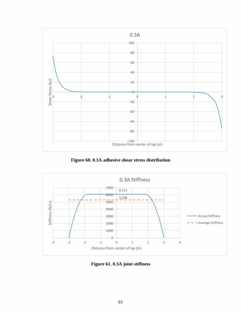
Figure 60. 0.3A adhesive shear stress distribution ....................................................................... 61

viii
Figure 61. 0.3A joint stiffness ...................................................................................................... 61
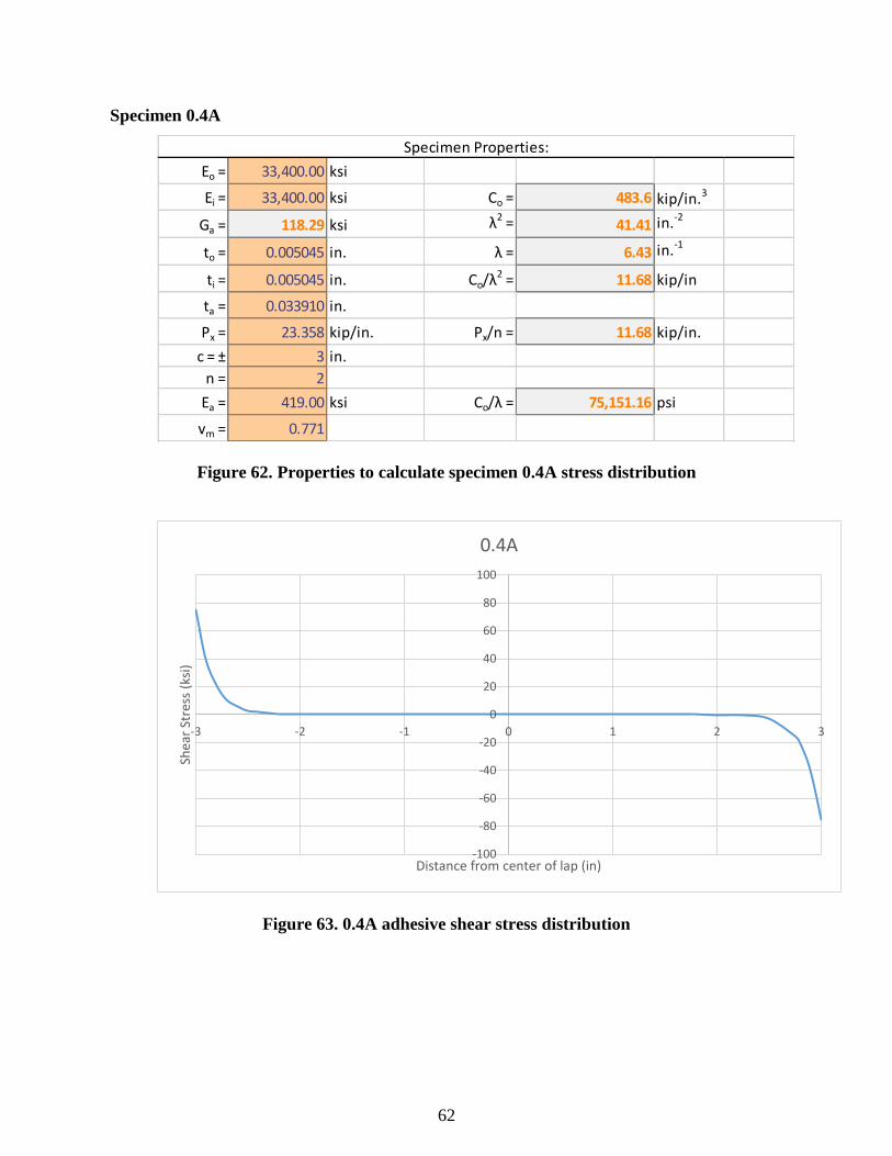
Figure 62. Properties to calculate specimen 0.4A stress distribution ........................................... 62
Figure 63. 0.4A adhesive shear stress distribution ....................................................................... 62
Figure 64. 0.4A joint stiffness ...................................................................................................... 63
Figure 65. Properties to calculate specimen 1.3 stress distribution .............................................. 63
Figure 66. 1.3 adhesive shear stress distribution .......................................................................... 64
Figure 67. 1.3 joint stiffness ......................................................................................................... 64
Figure 68. Properties to calculate specimen 1.4 stress distribution .............................................. 65
Figure 69. 1.4 adhesive shear stress distribution .......................................................................... 65
Figure 70. 1.4 joint stiffness ......................................................................................................... 66
Figure 71. Properties to calculate specimen 1.5 stress distribution .............................................. 66
Figure 72. 1.5 adhesive shear stress distribution .......................................................................... 67
Figure 73. 1.5 joint stiffness ......................................................................................................... 67
Figure 74. Properties to calculate specimen 1.6 stress distribution .............................................. 68
Figure 75. 1.6 adhesive shear stress distribution .......................................................................... 68
Figure 76. 1.6 joint stiffness ......................................................................................................... 69
Figure 77. Properties to calculate specimen 2.1 stress distribution .............................................. 69
Figure 78. 2.1 adhesive shear stress distribution .......................................................................... 70
Figure 79. 2.1 joint stiffness ......................................................................................................... 70
Figure 80. Properties to calculate specimen 2.2 stress distribution .............................................. 71
Figure 81. 2.2 adhesive shear stress distribution .......................................................................... 71
Figure 82. 2.2 joint stiffness ......................................................................................................... 72
Figure 83. Properties to calculate specimen 2.3 stress distribution .............................................. 72
Figure 84. 2.3 adhesive shear stress distribution .......................................................................... 73
Figure 85. 2.3 joint stiffness ......................................................................................................... 73
ix
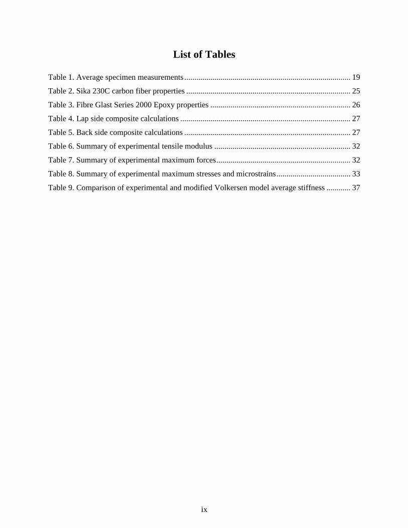
List of Tables
Table 1. Average specimen measurements ................................................................................... 19
Table 2. Sika 230C carbon fiber properties .................................................................................. 25
Table 3. Fibre Glast Series 2000 Epoxy properties ...................................................................... 26
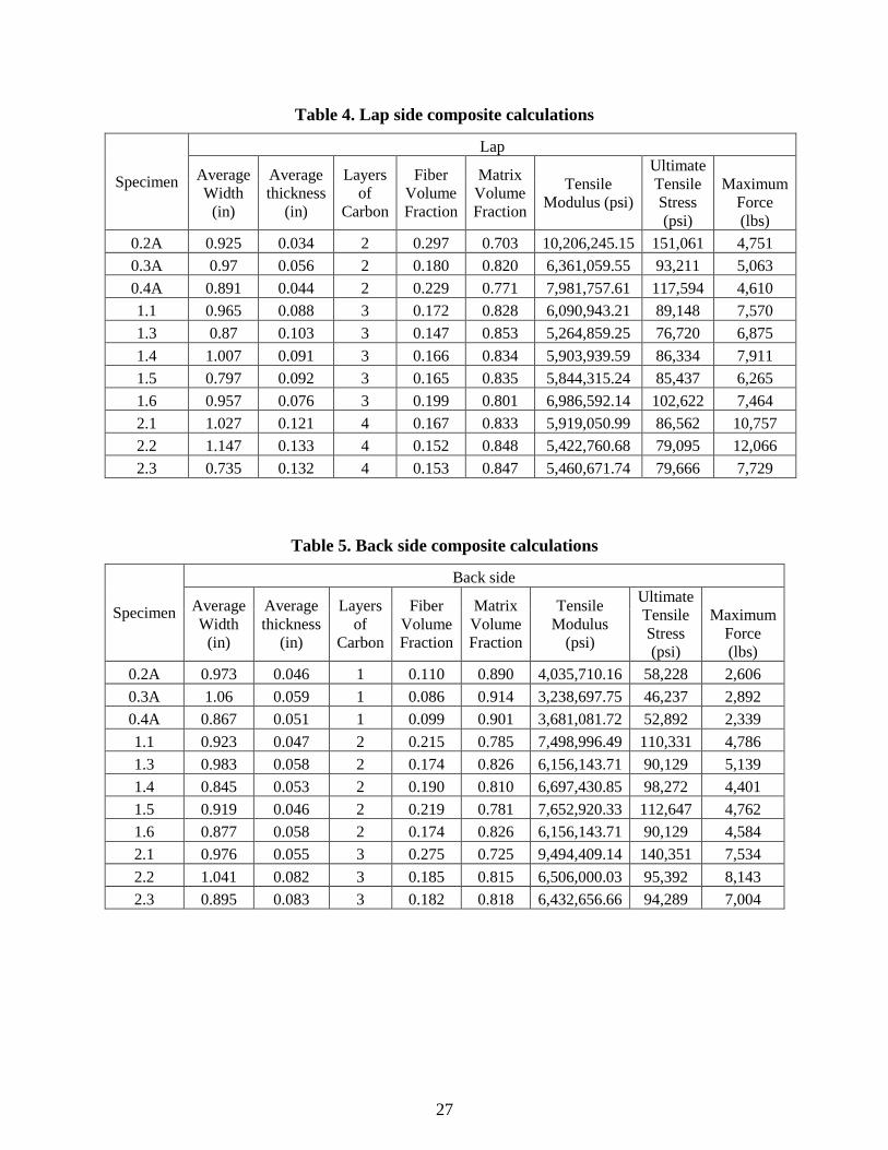
Table 4. Lap side composite calculations ..................................................................................... 27
Table 5. Back side composite calculations ................................................................................... 27
Table 6. Summary of experimental tensile modulus .................................................................... 32
Table 7. Summary of experimental maximum forces ................................................................... 32
Table 8. Summary of experimental maximum stresses and microstrains ..................................... 33
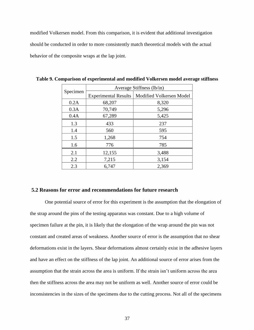
Table 9. Comparison of experimental and modified Volkersen model average stiffness ............ 37

x
Acknowledgements
Thank you to Dr. Phillippi for his guidance through my entire graduate curriculum.
Thank you to Dr. Hayder Rasheed and Fred Hasler for their guidance as my committee members.
Thank you my family for always supporting me and helping me through school. Lastly, thank
you to Suzy for your support, love, and understanding as I went through this process.

xi
Symbols List
P
Δ
L
A
E σ
ε
n
τ
λ
C0
x
c
Ga
ta
ti
to
Ei
Eo
wavg
tavg
Ef
Em
Vf
Vm
σTl,ult
Applied load
Change in length
Length
Area
Young’s modulus
Stress
Strain
Number of layers in lap
Shear stress
Elongation parameter
Adhesive stiffness parameter
Location along lap
Half of the lap length
Adhesive shear modulus
Adhesive thickness
Inner adherend thickness
Outer adherend thickness
Inner adherend Young’s modulus
Outer adherend Young’s modulus
Average width
Average thickness
Fiber tensile Young’s modulus
Matrix tensile Young’s modulus
Fiber volume fraction
Matrix volume fraction
Ultimate tensile stress

1
Chapter 1 - Introduction
Bonded composites have been used extensively in the aerospace and defense industries
since the 1940s and 50s. In the last three decades, civil and structural engineers have begun using
them on structures as a means of retrofit. Many structures require retrofitting because of
advances in the understanding of structural behavior during seismic events. Bonded composites
are used in structures to strengthen slabs, beams, and columns. Other methods of retrofitting
structures, such as steel jacketing of columns, have been around much longer in the field, but the
use of composites has many advantages over other methods. Primarily, composites have a high
strength-to-weight ratio, making them ideal for seismic retrofitting applications.
Composite wraps are often applied to columns to strengthen them against a seismic event.
The wraps provide column confinement and increase column ductility. However, while much is
known about the overall behavior of these column wraps, less information is available on the
behavior of the lap-joints of the wraps. The lap-joint is the location where the composite wrap
begins and ends. Composite wraps are often applied in many layers to a column without knowing
the effect of multiple layers on lap-joint behavior. Single-lap joints have been the focus of many
studies, dating back to the 1930s with Volkersen, but multi-lap joints have not been subject to
investigation in the same frequency that single-lap joints have. Multi-lap joints are lap joints with
one or more continuous layers through the joint. The purpose of this study is to better understand
the effect of having one and two continuous layers through the lap on the stiffness of CFRP
composite lap joints.
2
Chapter 2 - Literature Review
Bonded composites have been in use for decades. During the second World War, the
United States military began using glass fiber reinforced polymer composite vehicles in order to
make the vehicles lighter and save steel (Palucka & Bensaude-Vincent, 2002). After World War
II, the use of composites expanded into markets outside of the military. Beginning in the 1950’s,
composite materials experienced widespread use in the aerospace industry (Rasheed, 2015).
Fiber reinforced polymers (FRP) were utilized to produce airplane and rocket components and
motor casings. In addition to the aerospace industry, composites are used in the automotive,
marine, offshore drilling, sporting equipment, and civil engineering industries. Within the civil
engineering field, composite materials are often used to strengthen and retrofit reinforced
concrete slabs, beams, and columns.
A composite material is a combination of two separate materials to form a single unit.
The most commonly used composite material in civil engineering for retrofitting reinforced
concrete structures is the polymer matrix composite. Polymer matrix composites consist of two
primary ingredients: the matrix and the reinforcement (Kaw, 1997). Epoxy resin is the most
common matrix. Glass fibers, carbon fibers, and aramid fibers can all be used as reinforcement in
polymer matrix composites. The focus of this thesis will be on carbon fiber reinforced polymers
because they are less costly than aramid fibers, stronger than glass fibers, and are the most
frequently used type of fiber in the civil engineering industry.
Polymer matrix composites, henceforth known as composites, are an anisotropic
material—the material properties are different in each direction of the material. This is the
largest difference between composites and other materials, such as steel plates or bars. Steel
plates are isotropic and have the same material properties (modulus of elasticity, allowable
3
stresses, etc.) in each direction. Additionally, anisotropic materials have 21 independent elastic
constants in their stiffness matrix, while isotropic materials only have two, meaning it is much
easier to establish the stress-strain relationship for any particular point in an isotropic material
(Kaw, 1997). The matrix and reinforcement of a composite are combined to form a lamina. A
lamina is a single layer, or ply, and composites are typically constructed from multiple plies,
which form a laminate.
There are many advantages to using composite materials to retrofit reinforced concrete
columns over other options, such as steel jacketing. First, composite column wraps increase the
column’s ductility without making the column stiffer. Column ductility increases because of
confinement provided by the wrap. Increasing column ductility without increasing stiffness is
beneficial because during seismic events stiffer elements attract more load. Because composite
wraps do not increase column stiffness, the column does not attract additional load. Another
advantage associated with composite wraps is they don’t appreciably increase a structure’s
weight. Composites have a high strength-to-weight ratio, which means they help strengthen
structures without increasing their weight. This is important because if the weight of the structure
increases, the seismic forces acting on the structure increase and the columns may have to be
redesigned to make sure they can withstand the new lateral load.
There are two primary disadvantages when considering composite materials. The first
being the relatively high cost associated with the material. The second being the perceived lack
of durability. Composite materials need to be protected because they have effectively no
resistance to the high temperatures associated with a fire. If a column wrap is exposed to flames,
the matrix phase, or epoxy, will melt and the wrap will become ineffective. That being said, the

4
wrap may be replaced after a fire. Additionally, the composites should be protected from impact
to avoid fiber breakage.
2.1. Single-lap Joints
Single-lap joints are created using an adhesive layer to connect two adherends. Figure 1
shows a typical single-lap joint. Adhesive bonding is an alternative to mechanical bonding that
avoids the use of drilled holes and reduces stress concentrations (Tsai & Morton, 2010).
However, stress concentrations do still exist at the end of each adherend. The two types of
stresses occurring in an adhesively bonded joint are transverse normal tensile (peel) stress and
shear stress.
Figure 1. Single-lap joint geometry
Due to a sudden change in stiffness, stress concentrations occur at the lap location with
the maximum stresses occurring at the overlap ends (Panigrahi & Pradhan, 2009). If a spew fillet
is present at the ends of the adherends, the maximum adhesive stresses have been shown to be
much lower than if the ends are squared off as they are in Figure 1 (Lempke, 2013). Figure 2
shows an example of a single-lap joint with a spew fillet on the adherend ends.

5
Figure 2. Single-lap joint with spew fillet
Several other parameters also have an impact on the stress distributions and strength of a
single-lap joint. These parameters include the Young’s Modulus, the shear modulus, and the
Poisson’s Ratios for the adherend and adhesive. The most efficient design of a single-lap joint is
one such that the stiffness of each adherend is the same, meaning the joint is balanced. A
balanced joint exhibits the lowest possible value of peak adhesive peel stress for any lap
configuration (Kim & Kedward, 2002). Another factor affecting the stress distribution of the
joint is the thickness of the adhesive. As the thickness of the adhesive increases, the stresses at
the overlap ends increase (Lempke, 2013). This increase is because as the adhesive is made
thicker, the eccentricity of the load is higher which increases the force on the bonding region of
the single-lap joint. Additionally, increasing the Young’s Modulus of the adhesive increases the
stress at the overlap ends because the adhesive becomes stiffer and deforms less, which forces
more stress and deformation into the adherends.
Adhesively bonded joints have two areas of concern. The bond shear strength, which is
the load when shear failure occurs, and bond peel strength, which is the load when peel or
tension failure occurs (Tong, 1996). Panigrahi and Pradhan (2009) found that in a single-lap
joint, the adherends are likely to fail due to peel stresses before the adhesive layer fails. This is
due to the low transverse tensile strength of a single-lap composite joint.

6
The two most widely used solutions for single-lap joints are the Volkersen solution and
the Goland and Reissner solution. The first method for analyzing single-lap joints was proposed
by Volkersen in 1938. He proposed a simple shear lag model based on the assumption of one-
dimensional bar-like adherends with only shear deformation in the adhesive layer (Tsai,
Oplinger, & Morton, 1998). The Volkersen model is based on five assumptions:
1) a constant bond and adherend thickness
2) uniform distribution of shear strain through the adhesive thickness
3) the adhesive carries only out-of-plane stresses while the adherends carry only
in-plane stresses
4) linear elastic material behavior
5) deformation of the adherends in the out-of-plane direction is negligible
Goland and Reissner proposed their beam-on-elastic-foundation model in 1944. This
model simulated the joint as being comprised of two beams bonded with a shear- and transverse
normal-deformable layer (Tsai, Oplinger, & Morton, 1998). Tsai, Oplinger, and Morton (1998)
were able to provide a better prediction of adhesive shear stress distribution than Goland and
Reissner by including the adherend shear deformation in their analysis. The adherend shear
deformation was accounted for in Tsai, Oplinger, and Morton’s solution by assuming a linear
shear stress through the adherend thickness.
During the 1970’s, Hart-Smith developed an elastic-plastic model to predict the stresses
in single-lap joints. In the research, Hart-Smith identified the strain energy density per unit bond
area as the necessary parameter to establish the maximum bond strength achievable by the
adhesive (Hart-Smith, 1973). Lempke (2013) discusses how, in the early 1990’s, Tsai-Morton
discovered that Hart-Smith’s model was most accurate in predicting the stresses in short single-
7
lap joints. Short single-lap joints are defined as joints with a free adherend length to bonding
length ratio of less than 0.75.
In 1996, Tong conducted a study into the bond strength for adhesively-bonded single-lap
joints and found two main points. First, he showed that “the product of the strain energy density
and the adhesive thickness is equal to the mixed-mode energy release rate for an adhesive
bonded specimen.” Second, he showed that “the strain energy density ratio is the same as the
mode ratio of the mixed mode I and mode II fracture.”
Strain energy density is a measure of the strain energy per unit of volume and is related to
the stress and modulus of elasticity of the material. The energy release rate describes the rate at
which a crack propagates through a solid material and is the sum of the energy needed to break
the atomic bonds and the stored mechanical strain energy. For short crack lengths, the total
energy of the object increases with an increasing crack length, meaning an increasing force must
be acting on the object to grow the crack. Additional energy is required to be put into the object
to lengthen the crack until the atoms become separated enough that they are no longer attracted
to one another. For long cracks, an increase in crack length decreases the total amount of energy
in the system, which means the crack grows without the application of additional force.
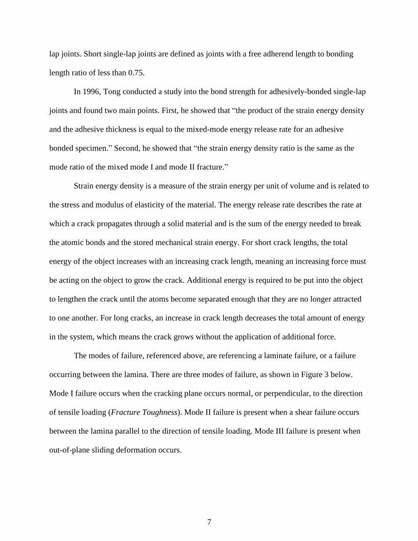
The modes of failure, referenced above, are referencing a laminate failure, or a failure
occurring between the lamina. There are three modes of failure, as shown in Figure 3 below.
Mode I failure occurs when the cracking plane occurs normal, or perpendicular, to the direction
of tensile loading (Fracture Toughness). Mode II failure is present when a shear failure occurs
between the lamina parallel to the direction of tensile loading. Mode III failure is present when
out-of-plane sliding deformation occurs.

8
Figure 3. Failure modes of laminate
In addition to the three types of laminate failure, there are three types of lamina failure
(Kaw, 1997). The three types of individual ply failure for a unidirectional lamina under
longitudinal tensile loading, shown in Figure 4, are (1) brittle fracture of fibers, (2) brittle
fracture of fibers with pullout, and (3) fiber pullout with fiber-matrix debonding. The type of
failure depends on the bond strength between the fiber and the matrix and the fiber volume
fraction. Brittle fracture of fibers occurs for low fiber volume fractions (less than 0.4); Brittle
fracture with fiber pullout occurs for fiber volume fractions ranging from 0.4 to 0.65; and fiber
pullout with debonding occurs when the fiber volume fraction is greater than 0.65. The fiber
volume fraction is a ratio of the volume of the fibers to the total volume of the composite.

9
Figure 4. Failure modes of unidirectional lamina in longitudinal tension
Tong again performed a study in 1998 in which a solution predicting the strengths of
adhesively bonded unbalanced single-lap joints with nonlinear adhesive properties was found.
His procedure consisted of a global/local analysis similar to that developed by Goland and
Reissner. Tong found that when subjected to a given load, the bond strain energy rate at the ends
of the overlap can be computed in terms of the membrane forces and the bending moments.
Overall, Tong showed that “neglecting the terms related to the transverse shear forces had a
slight effect on predictions of both [shear and peel] strain energy rates when the adhesive is
relatively flexible, and tended to yield a noticeable effect on both strain energy rates when the
adhesive is relatively stiff.”
10
2.2. Double-lap Joints
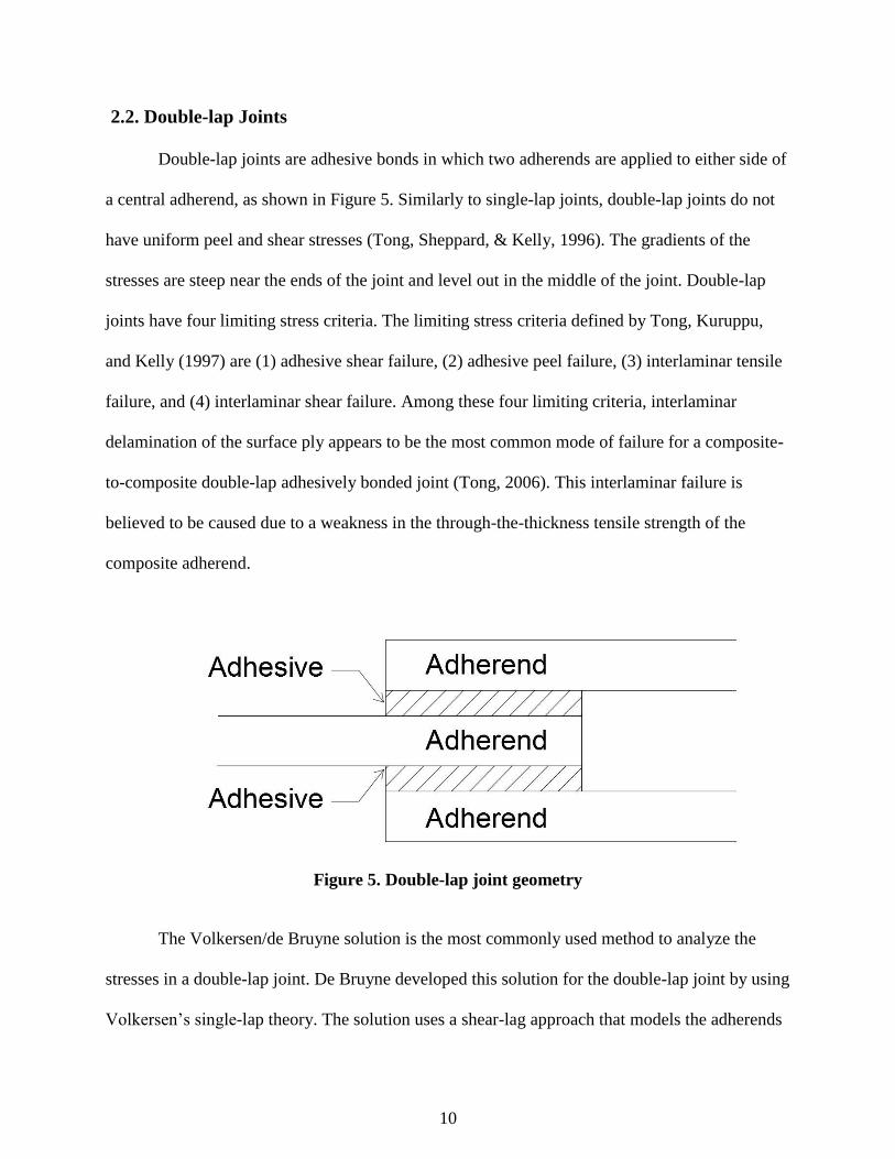
Double-lap joints are adhesive bonds in which two adherends are applied to either side of
a central adherend, as shown in Figure 5. Similarly to single-lap joints, double-lap joints do not
have uniform peel and shear stresses (Tong, Sheppard, & Kelly, 1996). The gradients of the
stresses are steep near the ends of the joint and level out in the middle of the joint. Double-lap
joints have four limiting stress criteria. The limiting stress criteria defined by Tong, Kuruppu,
and Kelly (1997) are (1) adhesive shear failure, (2) adhesive peel failure, (3) interlaminar tensile
failure, and (4) interlaminar shear failure. Among these four limiting criteria, interlaminar
delamination of the surface ply appears to be the most common mode of failure for a composite-
to-composite double-lap adhesively bonded joint (Tong, 2006). This interlaminar failure is
believed to be caused due to a weakness in the through-the-thickness tensile strength of the
composite adherend.
Figure 5. Double-lap joint geometry
The Volkersen/de Bruyne solution is the most commonly used method to analyze the
stresses in a double-lap joint. De Bruyne developed this solution for the double-lap joint by using
Volkersen’s single-lap theory. The solution uses a shear-lag approach that models the adherends
11
as bars and the adhesive as a shear spring. In this solution, the assumption is made that the
adherends do not have any shear deformation and that the adhesive layer carries only the shear
stresses in order to transfer the longitudinal forces from the inner to the outer adherends (Tsai &
Morton, 2010). Hart-Smith later showed that adhesive plasticity is a key player in determining
the bond shear strength for double-lap joints (Tong, Kuruppu, & Kelly, 1997).
In the previously discussed double-lap joint analyses shear deformation of the adherends
was ignored. However, large shear stresses would be present at the surfaces of the adherends
next to the adhesive layer because the adhesive layer withstands large shear stresses during load
transfer. The large shear stresses at the interface between the adhesive and adherend layers cause
the adherend to undergo shear deformation (Tsai, Oplinger, & Morton, 1998). This is especially
true for adherends with a low transverse shear modulus. Tsai, Oplinger, and Morton (1998)
provided a solution that improves upon the Volkersen/de Bruyne theory by considering the
adherend shear deformation in the analysis of double-lap joints by assuming a linear stress/strain
through the thickness of the adherend. Additionally, Tsai, Oplinger, and Morton (1998) showed
that for relatively large values of the transverse shear modulus and relatively small values of
adherend thickness, the adherend shear deformations may be ignored and the Volkersen/de
Bruyne solution reasonably predicts the adhesive shear stress.
In 2010, Tsai and Morton showed that the assumption of zero adherend shear stress made
by the Volkersen/de Bruyne solution is not valid. Tsai and Morton showed that the Volkersen/de
Bruyne solution predicted maximum shear stress values 33% higher than those found during
their experiment (Tsai & Morton, 2010). Additionally, they showed that the Tsai, Oplinger, and
Morton solution, discussed previously, provides a good prediction of the normalized adhesive
shear strain distribution for both a unidirectional and a quasi-isotropic joint. Also documented
12
were the typical failure modes for the unidirectional and quasi-isotropic joints. Both joints were
found to fail at the end of the strap with cohesive failure occurring in the unidirectional joint and
delamination at the first ply occurring in the quasi-isotropic joint.
In 1994, Tong performed a study on double-lap joints and developed equations relating
the maximum load that can be applied to the maximum strain energy density obtainable in shear
in the adhesive (Tong, 1994). That study also showed that for stiffness balanced joints, shear
failure occurs at both ends of the overlap. However, an imbalance in stiffness will cause the
shear failure to occur at one end of the overlap, and, thus, decrease the overall bond strength of
the joint. Another important parameter to consider is nonlinear adhesive behavior. This behavior
becomes important when an applied load is large enough to create plastic zones at each end of
the adhesive layer (Tong, Kuruppu, & Kelly, 1997). For composite double-lap joints, linear
analyses predicted failure loads far less than those measured by Tong, Kuruppu, and Kelly
(1997), while their nonlinear analysis seemed to give a good prediction of the failure load.
For the analysis of a more practical real world scenario, Tong, Sheppard, and Kelly
(1996) investigated the effect of adherend alignment on the behavior of adhesively bonded
double-lap joints. In the manufacturing of double-lap joints it is difficult to perfectly align the
ends of the outer adherends. The analysis of end mismatch, as shown in Figure 6, showed that
local bending is caused which, as described by Tong, “has an effect on the surface normal
displacement of the outer adherend and stresses in the adhesive layer.” An increase in peel stress
due to the end mismatch is undesirable because it may cause premature failure of the joint. In
order to account for end mismatch, Tong, Sheppard, and Kelly developed a modified formula
that characterizes the peel stress in terms of surface normal displacement.

13
Figure 6. Lap-joint with end mismatch

14
Chapter 3 - Experiment
3.1 Problem description
The situation explored for this thesis is a lap-joint with one and two continuous middle
layers. Figure 7 shows a lap-joint with one continuous middle lamina and Figure 8 shows a lap-
joint with two continuous laminas. These geometries require investigation because no previous
experimentation has been done on a lap-joint with a similar geometry. The purpose of this
investigation is to determine what effect the continuous middle lamina(s) may have on the
stiffness of the lap-joint and if stress concentrations occur due to a change in stiffness at the lap
joint.
Figure 7. Lap-joint with one continuous middle layer
Figure 8. Lap-joint with two continuous middle layers
15
Carbon fiber reinforced polymer wraps are often used in civil engineering around
reinforced concrete columns. In the field, a wrap will likely be applied continuously around the
column multiple times. Understanding the actual stiffness of the lap-joint will play a crucial role
in understanding the behavior of the interaction between the column and the wrap.
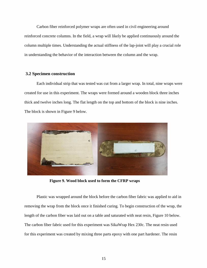
3.2 Specimen construction
Each individual strip that was tested was cut from a larger wrap. In total, nine wraps were
created for use in this experiment. The wraps were formed around a wooden block three inches
thick and twelve inches long. The flat length on the top and bottom of the block is nine inches.
The block is shown in Figure 9 below.
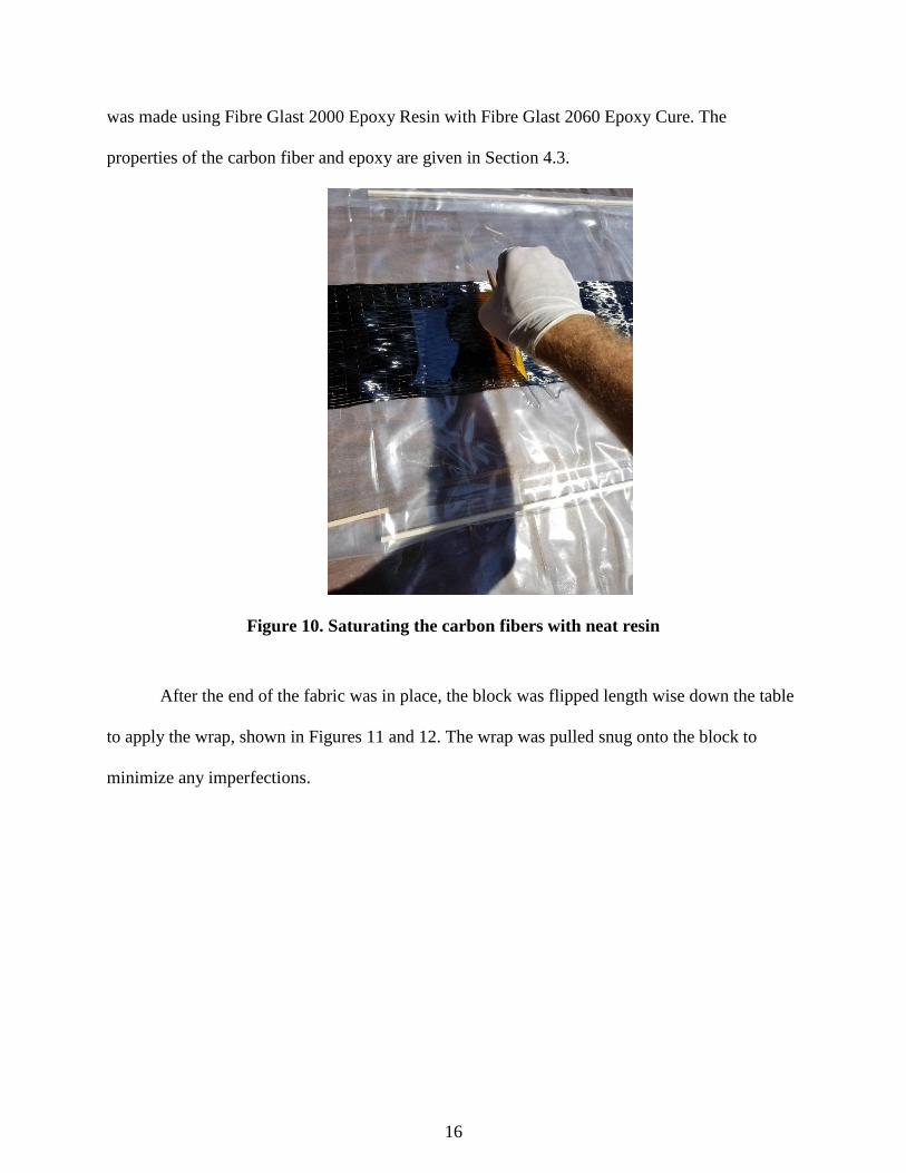
Plastic was wrapped around the block before the carbon fiber fabric was applied to aid in
removing the wrap from the block once it finished curing. To begin construction of the wrap, the
length of the carbon fiber was laid out on a table and saturated with neat resin, Figure 10 below.
The carbon fiber fabric used for this experiment was SikaWrap Hex 230c. The neat resin used
for this experiment was created by mixing three parts epoxy with one part hardener. The resin
Figure 9. Wood block used to form the CFRP wraps
16
was made using Fibre Glast 2000 Epoxy Resin with Fibre Glast 2060 Epoxy Cure. The
properties of the carbon fiber and epoxy are given in Section 4.3.
Figure 10. Saturating the carbon fibers with neat resin
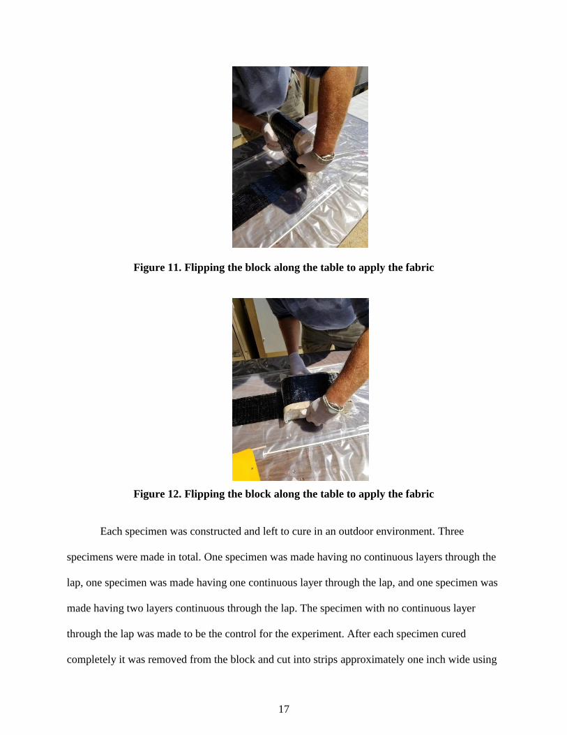
After the end of the fabric was in place, the block was flipped length wise down the table
to apply the wrap, shown in Figures 11 and 12. The wrap was pulled snug onto the block to
minimize any imperfections.
17
Figure 11. Flipping the block along the table to apply the fabric
Figure 12. Flipping the block along the table to apply the fabric
Each specimen was constructed and left to cure in an outdoor environment. Three
specimens were made in total. One specimen was made having no continuous layers through the
lap, one specimen was made having one continuous layer through the lap, and one specimen was
made having two layers continuous through the lap. The specimen with no continuous layer
through the lap was made to be the control for the experiment. After each specimen cured
completely it was removed from the block and cut into strips approximately one inch wide using

18
a tile saw, which can be seen in Figures 13 and 14 below. Specimens were cut into one inch
strips to follow the requirements of ASTM D3039, described in section 3.4. Three single-lap
strips, five strips with one continuous layer, and five strips with two continuous layers were cut
and tested.
Figure 13. Saw used to cut specimens
Figure 14. Saw used to cut specimens

19
3.3 Specimen properties
After cutting each specimen into strips, measurements were taken to determine an
average width and thickness of the lap side and the back side of the specimen. The side with the
lap joint is being called the lap side and the side opposite the lap-joint is considered as the back
side. Averages were determined by taking measurements in three places along the lap and three
places along the back side. The average measurements for each specimen are given in Table 1.
Table 1. Average specimen measurements
Specimen L.S. wavg
(in)
B.S. wavg
(in)
Lap tavg
(in)
B.S. tavg
(in)
0.1A 0.903 0.881 0.052 0.025
0.2A 0.925 0.973 0.034 0.046
0.3A 0.97 1.06 0.056 0.059
0.4A 0.891 0.867 0.044 0.051
1.1 0.965 0.923 0.088 0.047
1.3 0.87 0.983 0.103 0.058
1.4 1.007 0.845 0.091 0.053
1.5 0.797 0.919 0.092 0.046
1.6 0.957 0.877 0.076 0.058
2.1 1.027 0.976 0.121 0.055
2.2 1.147 1.041 0.133 0.082
2.3 0.735 0.895 0.132 0.083
2.4 0.852 1.009 0.127 0.063
2.6 0.926 0.977 0.122 0.075
L.S. = Lap side
B.S.= Back side
w = Width
t = Thickness
3.4 Test set-up
Each specimen was attached to two three inch diameter steel pins and tested in tension.
One of the steel pins is shown in Figure 15. The strips were pulled at a displacement rate of 0.05
inches per minute in accordance with ASTM D3039. ASTM D3039 is the standard most

20
applicable to the testing performed for this experiment. The tests for this experiment were
performed on continuous strips of a polymer matrix composite whereas ASTM D3039 is
designed for tensile tests on polymer matrix composite coupons.
Each test was done on the MTS 810 Material Test System machine. During the test,
strain gauges were placed in three locations. Strain gauge one was placed on the lap near the end;
strain gauge two was placed on the lap side of the specimen outside of the lap; and, strain gauge
three was placed on the back side of the specimen. Strain gauge locations are shown in Figure
18. The strain was used to determine the stiffness of the composite wrap as will be described in
section 4.1.
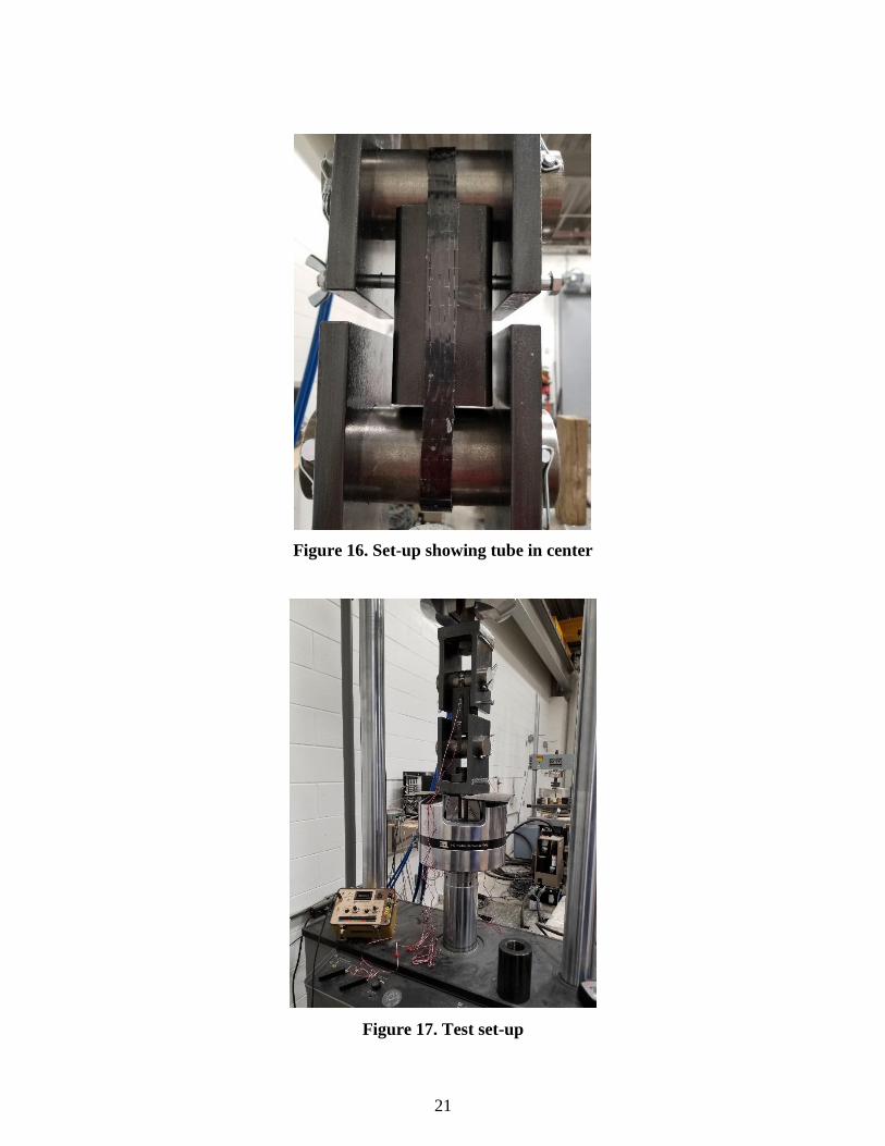
A hollow metal tube was placed between each of the steel pins to limit inward rotation of
the test specimen. In a real world application against a concrete column, the wrap will not be
able to rotate inward towards its center because the concrete will be pushing it outward. The tube
can be seen between the pins in Figure 16. An overall set-up of the experiment is shown in
Figure 17.
Figure 15. Steel pin used for tensile test
21
Figure 16. Set-up showing tube in center
Figure 17. Test set-up

22
Chapter 4 - Theoretical Models
4.1 Stiffness equation model
The purpose of this research is to relate strain to an average stiffness, Kavg, in order to
determine the stiffness of a CFRP wrap with a certain number of layers and a six inch lap length.
Figure 18. Experimental set-up
Figure 19. Free body diagram of CFRP around pin
From the free body diagram,
𝑃 = 𝑃1 + 𝑃2 (1)

23
For these calculations, it is assumed that compared to the rest of the strap, the elongation around
the pins is relatively constant and therefore negligible. From this assumption, the change in
length of the wrap is given by
∆1=
𝑃1𝐿1𝐸1𝐴1
(2)
∆2=
𝑃2𝐿2𝐸2𝐴2
(3)
where,
L1=total length minus the lap length, 3”
L2= total length, 9”
And, A1≈A2 and E1≈E2. From this relationship equation 3 can be rewritten as
∆2=
𝑃2𝐿2𝐸1𝐴1
(3.1)
The average stress over the section is given by
𝜎1 =
𝑃1𝐴1
(4)
𝜎2 =
𝑃2𝐴2=𝑃2𝐴1
(5)
The stress over the section is also given by
𝜎1 = 𝐸1𝜀1 (6)
𝜎2 = 𝐸1𝜀2 (7)
By solving equations 4 and 5 for the force and substituting into equation 1:
𝑃 = 𝜎1𝐴1 + 𝜎2𝐴1 (8)

24
From substituting equations 6 and 7 into equation 8 and simplifying, the following expression
can be found for the total tensile force in the wrap.
𝑃 = 𝐸1𝐴1(𝜀1 + 𝜀2) (9)
If area three is over the length of the lap, it follows that
𝑃1 = 𝑃3 (10)
∆3=
𝑃3𝐿3𝐸𝑎𝑣𝑔𝐴3
(11)
where,
L3= length of the lap, 6”
Eavg= average stiffness of the lap
From equation 10, it follows that
𝑃3 = 𝐸1𝜀1𝐴1 (12)
By plugging equation 12 into equation 11 and rearranging, an expression for the average
stiffness of the lap joint is given by equation 13.
𝐸𝑎𝑣𝑔𝐴3
𝐿3= 𝑘𝑎𝑣𝑔 =
𝐸1𝜀1𝐴1∆3
(13)
4.2 Modified Volkersen model
For the theoretical analysis the shear-lag based solution proposed by Volkersen was used
with modifications to account for the middle continuous laminas. The equations used to
determine the shear stress through the lap are given in equations 14 through 16. The number of
layers through the lap is given by n. n should include both outer adherends and all of the inner
adherends continuing through the lap. The (n-1) term was added to the elongation parameter, λ2,
and the C0 equation. If the number of layers is input as two, i.e. no continuous lamina through the

25
lap, Volkersen’s original equations are recovered. The terms related to the stiffness of the lap
joint are C0 and λ2. The purpose of the modified Volkersen model is to find a way to determine
the stiffness of the joint and match it with the stiffness given by equation 13.
𝜏(𝑥) = 𝜆 [(
𝑃𝑥𝑛−𝐶0𝜆2)𝑠𝑖𝑛ℎ( 𝜆𝑥)
𝑐𝑜𝑠ℎ( 𝜆𝑐)+𝑃𝑥𝑛(𝑐𝑜𝑠ℎ(𝜆𝑥)
𝑠𝑖𝑛ℎ(𝜆𝑐))]
(14)
𝜆2 =
𝐺𝑎𝑡𝑎(1
𝐸𝑜𝑡𝑜+
1
𝐸𝑖𝑡𝑖(𝑛 − 1))
(15)
𝐶0 =
𝐺𝑎𝑃𝑥𝐸𝑖𝑡𝑖(𝑛 − 1)𝑡𝑎𝑡𝑜
(16)
4.3 Specimen strength
Using the measurements listed in Table 1, the fiber volume fraction, matrix volume
fraction, tensile modulus, ultimate tensile stress, and maximum force were calculated for the lap
side and back side of each specimen. Each of the parameters listed was calculated using the
properties of the Sika 230C carbon fiber and Fibre Glast Series 2000 Epoxy, given in Tables 2
and 3.
Table 2. Sika 230C carbon fiber properties
Primary fiber direction 0° Unidirectional
Density 0.065 #/in3
Area weight 0.0003279 #/in2
Thickness per layer, Af 0.005045 in
Tensile strength, σult,t 5 x 10⁵ psi
Tensile elastic modulus, Ef 33.4 x 10⁶ psi
Elongation, εf 0.015 in/in

26
Table 3. Fibre Glast Series 2000 Epoxy properties
Property Neat Resin With Carbon
Density 0.0401 lb/in3
Tensile Strength,
σf,ultT 9828 psi --
Elongation at Break,
ε 0.019 in/in 0.0091 in/in
Tensile Modulus, Em 418,525 psi --
The amount of fiber is determined by the thickness per layer of carbon fiber
multiplied by the number of layers in the lap or back side. The fiber volume fraction is the
thickness of the fiber present divided by the average thickness of the location. The matrix
volume fraction is one minus the fiber volume fraction. The composite tensile modulus was
calculated using equation 17, the composite ultimate tensile stress was calculated using equation
18, and the maximum force was calculated using equation 19. The results of the calculations are
given in Table 4 for the lap side of the specimen and Table 5 for the back side of the specimen.
𝐸𝐿 = 𝐸𝑓𝑉𝑓 + 𝐸𝑚𝑉𝑚 (17)
𝜎𝑙,𝑢𝑙𝑡𝑇 = 𝜎𝑢𝑙𝑡,𝑡𝑉𝑓 + 𝜀𝑚𝑖𝑛𝐸𝑚𝑉𝑚 (18)
𝐹 = 𝜎𝑙,𝑢𝑙𝑡𝑇 𝑤𝑎𝑣𝑔𝑡𝑎𝑣𝑔 (19)
27
Table 4. Lap side composite calculations
Specimen
Lap
Average
Width
(in)
Average
thickness
(in)
Layers
of
Carbon
Fiber
Volume
Fraction
Matrix
Volume
Fraction
Tensile
Modulus (psi)
Ultimate
Tensile
Stress
(psi)
Maximum
Force
(lbs)
0.2A 0.925 0.034 2 0.297 0.703 10,206,245.15 151,061 4,751
0.3A 0.97 0.056 2 0.180 0.820 6,361,059.55 93,211 5,063
0.4A 0.891 0.044 2 0.229 0.771 7,981,757.61 117,594 4,610
1.1 0.965 0.088 3 0.172 0.828 6,090,943.21 89,148 7,570
1.3 0.87 0.103 3 0.147 0.853 5,264,859.25 76,720 6,875
1.4 1.007 0.091 3 0.166 0.834 5,903,939.59 86,334 7,911
1.5 0.797 0.092 3 0.165 0.835 5,844,315.24 85,437 6,265
1.6 0.957 0.076 3 0.199 0.801 6,986,592.14 102,622 7,464
2.1 1.027 0.121 4 0.167 0.833 5,919,050.99 86,562 10,757
2.2 1.147 0.133 4 0.152 0.848 5,422,760.68 79,095 12,066
2.3 0.735 0.132 4 0.153 0.847 5,460,671.74 79,666 7,729
Table 5. Back side composite calculations
Specimen
Back side
Average
Width
(in)
Average
thickness
(in)
Layers
of
Carbon
Fiber
Volume
Fraction
Matrix
Volume
Fraction
Tensile
Modulus
(psi)
Ultimate
Tensile
Stress
(psi)
Maximum
Force
(lbs)
0.2A 0.973 0.046 1 0.110 0.890 4,035,710.16 58,228 2,606
0.3A 1.06 0.059 1 0.086 0.914 3,238,697.75 46,237 2,892
0.4A 0.867 0.051 1 0.099 0.901 3,681,081.72 52,892 2,339
1.1 0.923 0.047 2 0.215 0.785 7,498,996.49 110,331 4,786
1.3 0.983 0.058 2 0.174 0.826 6,156,143.71 90,129 5,139
1.4 0.845 0.053 2 0.190 0.810 6,697,430.85 98,272 4,401
1.5 0.919 0.046 2 0.219 0.781 7,652,920.33 112,647 4,762
1.6 0.877 0.058 2 0.174 0.826 6,156,143.71 90,129 4,584
2.1 0.976 0.055 3 0.275 0.725 9,494,409.14 140,351 7,534
2.2 1.041 0.082 3 0.185 0.815 6,506,000.03 95,392 8,143
2.3 0.895 0.083 3 0.182 0.818 6,432,656.66 94,289 7,004

28
Chapter 5 - Results and Conclusion
5.1 Results
5.1.1 Experimental results
The data received from the testing machine used in the experiment was the total force the
machine was pulling with, the total displacement of the pulling apparatus, and the strain for all
three strain gauges. With the data provided from the machine, charts plotting force vs.
displacement, lap strain vs. displacement, off lap strain vs. displacement, and back side strain vs.
displacement were created. An example of these charts is shown below, in Figures 20 and 21.
Figure 20. Example of force vs. displacement chart using test data

29
Figure 21. Example of strain vs. displacement chart using test data
From the charts above, two points of displacement were chosen from the linear portion of
the graph. The two strains were chosen from the elastic portion of the graph to set the difference
in the chosen strains as the true strain for the specimen at that location. Then, calculations were
done to determine the forces P1 and P2 distributed to the off lap and back side, respectively, using
the following equations.
𝜀1 = 𝜀1𝑗 − 𝜀1𝑖 (20)
𝜀2 = 𝜀2𝑗 − 𝜀2𝑖 (21)
𝑃1 =
𝜀1𝐴1𝜀1𝐴1 + 𝜀2𝐴2
𝑃 (22)
𝑃2 =
𝜀2𝐴2𝜀1𝐴1 + 𝜀2𝐴2
𝑃 (23)
The lap stress was calculated using P1 divided by the average area of the lap, and then
plotted on a stress vs. strain chart. The off lap stress was calculated using P1 divided by the off
lap average area, and the back side stress was calculated using P2 and the average area of the
back side. Examples of the stress vs. strain charts are shown below, in Figure 22. From these

30
charts, the modulus of each area was determined using the slope of the chart from the linear
portion. Some of the charts have a portion of their strain data points in the negative region, as
seen in the example of off lap stress vs. strain chart. This is believed to be caused by curvature at
the lap joint. The lap joint is likely rotating outward, putting the surface in compression until the
overall tension force through the lap became high enough to overcome the compression. A
summary of the experimental tensile modulus results is given in Table 6, a summary of the
maximum forces is presented in Table 7, a summary of the stress and microstrain at the breaking
point is shown in Table 8, and all of the stress vs. strain charts for the specimens can be found in
Appendix A.

31
Figure 22. Example stress vs. strain curves

32
Table 6. Summary of experimental tensile modulus
Specimen Modulus (psi)
Lap Off Lap Back Side
0.2A 1,136,347 640,055 612,765
0.3A 758,396 469,153 275,207
0.4A 820,154 469,411 460,129
1.1 387,497 954,825 998,123
1.3 101,767 569,292 564,804
1.4 131,885 813,547 857,701
1.5 249,803 1,213,997 1,166,175
1.6 178,618 811,830 795,428
2.1 352,563 471,492 474,449
2.2 567,461 349,704 342,394
2.3 269,655 491,899 512,094
Table 7. Summary of experimental maximum forces
Specimen
At breaking point
Lap Side Back Side
P1max (lbf) P2max (lbf)
0.2A 1104.65 115.89
0.3A 1511.25 97.57
0.4A 1029.70 90.65
1.3 219.56 1891.48
1.4 435.76 3361.38
1.5 579.61 2868.37
1.6 442.55 2798.88
2.1 4711.13 2493.01
2.2 4858.80 3238.07
2.3 3698.61 4010.69

33
Table 8. Summary of experimental maximum stresses and microstrains
Specimen
At breaking point
Total Force
(lbf)
Displacement
(in)
Lap Peak Stress
(psi)
Off Lap Peak Stress
(psi)
Back Side Peak
Stress (psi)
Microstrain Microstrain Microstrain
0.2A 1220.54 0.0771 35,124 33,173 2,589
31,191 48,960 3,945
0.3A 1608.81 0.0936 27,821 33,149 1,560
33,918 71,569 5,316
0.4A 1120.35 0.0762 26,265 28,892 2,050
32,641 67,204 4,384
1.1 3430.09 0.1027 36,602 48,802 7,419
99,238 38,791 8,199
1.3 2111.04 0.0720 2,450 3,321 33,176
14,177 6,274 69,980
1.4 3797.14 0.1123 4,755 6,459 75,056
35,226 7,813 90,779
1.5 3447.98 0.1309 7,905 9,962 67,852
7,040 8,571 58,603
1.6 3241.43 0.0914 6,085 5,854 55,025
24,977 7,660 73,912
2.1 7204.14 0.1455 37,911 40,595 46,442
107,622 58,074 105,499
2.2 8096.87 0.1341 31,850 35,301 37,933
38,404 103,137 112,704
2.3 7709.30 0.1560 38,122 38,413 53,991
129,313 26,086 108,026
In order to determine the stiffness of each lap joint, an adjusted stress had to be calculated
by using an adjusted strain for the off lap strain gauge. An adjustment was made because
bending in the joint was causing forces which were either increasing or decreasing the value of
the strain from the normal stress. For specimens 0.2A, 0.3A, and 0.4A the off lap strain gauge
was placed in the tension region caused by the outward rotation of the joint. For these specimens,
the strain at the maximum load had to be reduced because the tension force from bending was
increasing the normal tensile force on the cross section. For specimens 1.3, 1.4, 1.5, 1.6, 2.1, 2.2,
and 2.3 the off lap strain gauge was placed in the compression region caused by outward rotation

34
at the joint. For these specimens, the strain at the maximum load had to be increased because the
compression force from bending decreased the normal tensile force. The strain of specimen 1.1
made it an outlier and it was ignored for all calculations. The adjusted strain at the specimen
breaking point was calculated using the following equations.
𝑒 = 0.145𝑡𝑜𝑓𝑓 𝑙𝑎𝑝 (24)
𝑀 = 𝑒𝑃1,𝑚𝑎𝑥 (25)
𝜎𝑎𝑑𝑗𝑢𝑠𝑡𝑒𝑑 =
𝑃1,𝑚𝑎𝑥𝐴𝑜𝑓𝑓 𝑙𝑎𝑝
+𝑀
𝑆
(26.1)
𝜎𝑎𝑑𝑗𝑢𝑠𝑡𝑒𝑑 =
𝑃1,𝑚𝑎𝑥𝐴𝑜𝑓𝑓 𝑙𝑎𝑝
−𝑀
𝑆
(26.2)
𝜀1,𝑎𝑑𝑗𝑢𝑠𝑡𝑒𝑑 = 𝜀1 (𝜎𝑎𝑑𝑗𝑢𝑠𝑡𝑒𝑑
𝜎) (27)
The value for the eccentricity of the load, e, was determined based on a ratio of an
assumed distance between the centerlines of the outer adherends and the thickness of the
specimen at the off lap joint. Equation 26.1 was used to determine the adjusted stress for
specimens 1.3, 1.4, 1.5, 1.6, 2.1, 2.2, and 2.3; and equation 26.2 was used to calculate the
adjusted stress for specimens 0.2A, 0.3A, and 0.4A.
From the adjusted strain on the lap side, the average stiffness of the lap was calculated
using equations 28 and 13.1, where L1 is assumed to equal three inches and L2 is assumed to
equal nine inches.
∆3= ∆2 − ∆1= 𝜀2𝐿2 − 𝜀1,𝑎𝑑𝑗𝑢𝑠𝑡𝑒𝑑𝐿1 (28)
(𝐸𝐴3𝐿3)𝑎𝑣𝑔
=𝐸1𝜀1,𝑎𝑑𝑗𝑢𝑠𝑡𝑒𝑑𝐴1
∆3
(13.1)
The value of E1 used for the above calculation is the value listed for the off lap modulus
in Table 6. When comparing the value of the modulus determined from experimental data, in
Table 6, with the value of the modulus when calculating it from the manufacturer’s data, in Table

35
4, it is clear to see that the experimental modulus is much lower. The difference in these values is
likely due to imperfect construction in less than ideal conditions. A summary of the lap average
stiffness is given after the discussion of the results from the modified Volkersen model.
5.1.2 Modified Volkersen model results
Using the equations given in Section 4.2, the value of the shear stress in the adhesive was
calculated at discrete points along the lap and plotted as a function of distance from the
centerline, as shown in Figure 23. The force used in the stress calculations was P1,max ,from the
experimental results. P1,max was divided by the total thickness of the lap. From Figure 23, the
area under the curve was calculated from the peak to the point at which the stress is zero. The
area under the curve is the total force transferred through the adhesive into the lap region. It can
be seen from the figure that the adhesive almost fully transfers the load to the outer adherend of
the lap after only about one half inch. For all of the specimens the area under the graph became
zero at a distance of just over one inch. Using the area under the curve and dividing it by the
distance along the curve until the stress is zero gives the maximum stiffness of the lap. Figure 24
shows an example of the stiffness of the lap determined using Figure 23. The average stiffness,
shown in Figure 24, was determined by dividing the area under the curve of the actual stiffness
by the total lap length of six inches. Charts of each specimen’s adhesive shear stress distribution
and average stiffness are given in Appendix B.

36
Figure 23. Example plot of adhesive shear stress vs. distance from the lap center point
Figure 24. Example plot of lap stiffness calculated from modified Volkersen model
Table 9 gives a summary of the average stiffness of the lap joint determined by the
experiment compared to that determined using the modified Volkersen model. It is obvious from
the table that discrepancies exist between the results of the experiment and the results from the
37
modified Volkersen model. From this comparison, it is evident that additional investigation
should be conducted in order to more consistently match theoretical models with the actual
behavior of the composite wraps at the lap joint.
Table 9. Comparison of experimental and modified Volkersen model average stiffness
Specimen Average Stiffness (lb/in)
Experimental Results Modified Volkersen Model
0.2A 68,207 8,320
0.3A 70,749 5,296
0.4A 67,289 5,425
1.3 433 237
1.4 560 595
1.5 1,268 754
1.6 776 785
2.1 12,155 3,488
2.2 7,215 3,154
2.3 6,747 2,369
5.2 Reasons for error and recommendations for future research
One potential source of error for this experiment is the assumption that the elongation of
the strap around the pins of the testing apparatus was constant. Due to a high volume of
specimen failure at the pin, it is likely that the elongation of the wrap around the pin was not
constant and created areas of weakness. Another source of error is the assumption that no shear
deformations exist in the layers. Shear deformations almost certainly exist in the adhesive layers
and have an effect on the stiffness of the lap joint. An additional source of error arises from the
assumption that the strain across the area is uniform. If the strain isn’t uniform across the area
then the stiffness across the area may not be uniform as well. Another source of error could be
inconsistencies in the sizes of the specimens due to the cutting process. Not all of the specimens

38
are the same width and not all of the specimens with the same number of lamina are the same
thickness due to the buildup of excess epoxy on the wraps.
Possible future research into multi-lap joints could include investigating different lap
lengths and their effect on joint stiffness and stress distribution. Additional research could also
be conducted on multi-layer laps using different models, such as the Hart-Smith Elastic-Plastic
model. Further research could also be conducted into the effect shear deformation within the
adhesive has on the joint stiffness. Another topic of future research could be additional
modifications to the Volkersen model with the modifications being included in the derivation of
the equations, rather than substituting a modification into the final equations. Lastly, once
experimental results have been successfully matched with theoretical model results the next step
would be to apply the composite to concrete cylinders to see if the behavior of the composite is
changed because of its application to concrete.
5.3 Conclusion
Composite lap joints are important for the civil engineering industry. They are present
when concrete columns in existing structures have been retrofitted for better seismic
performance by applying a composite wrap. While using CFRP composite wraps is a popular
method for retrofitting reinforced concrete columns and much is known about their overall
behavior, less information is available on how multi-layer lap joints effect the behavior of the
wrap. Wrapping layers of fabric around the column multiple times creates a multi-lap joint
between the beginning and termination of the wrap.
The subject of this research was lap joints with multiple continuous laminas through the
lap. The aspect of interest for this investigation was determining the stiffness of the lap joint in

39
order to examine how stress concentrations may affect the joint. To determine the stiffness of lap
joints with zero, one, and two continuous laminas through the lap, tests were performed on
specimens constructed of carbon fiber and epoxy. From these tests, experimental values of the
average stiffness of the lap joint for each configuration were calculated and compared to a
theoretical model that was intuitively modified to account for the continuous layers through the
lap. While no definitive conclusion could be drawn from the study performed, results of this
study may be used by future researchers to refine the equations presented so that a computational
model can be formulated that accurately predicts actual lap behavior.

40
References
Hart-Smith, L.J. (1973). Adhesive-bonded double-lap joints. NASA CR-112235
Fracture Toughness. Retrieved from https://www.nde- ed.org/EducationResources/
CommunityCollege/Materials/Mechanical/FractureToughness.php
Kaw, A. (1997). Mechanics of Composite Materials. Boca Raton, FL: CRC Press.
Kim, H., & Lee, J. (2004). Adhesive nonlinearity and the prediction of failure in bonded
composite lap joints. Joining and Repair of Composite Structures, ASTM STP 1455, K.T.
Kedward and H. Kim, Eds., ASTM International, West Conshohocken, PA.
Lempke, M (2013). A study of single-lap joints (Master’s thesis, Michigan State University). Retrieved from https://d.lib.msu.edu/etd/2280/datastream/OBJ/download/A_study_of_single-
lap_joints.pdf
Palucka, T., & Bensaude-Vincent, B. (2002, October 19). Composites Overview. Retrieved from
http://authors.library.caltech.edu/5456/1/hrst.mit.edu/hrs/materials/public/composites/Comp
osites_Overview.htm
Rasheed, H. A. (2015). Strengthening design of reinforced concrete with FRP. Boca Raton, FL:
CRC Press.
Tong, L. (2006). An analysis of failure criteria to predict the strength of adhesively bonded
composite double lap joints.
Tong, L., Kuruppu, M., & Kelly, D. (1997). Analysis of adhesively bonded composite double lap
joints. Journal of Thermoplastic Composite Materials, 10, 61-75.
Tong, L (1994). Bond shear strength for adhesive bonded double-lap joints. International
Journal of Solids Structures, 31, 2919-2931.
Tong, L (1996). Bond strength for adhesive-bonded single-lap joints. Acta Mechanica, 117, 101-
113.
Tong. L., Sheppard, A., & Kelly, D. (1996). Effect of adherend alignment on the behavior of
adhesively bonded double lap joints. International Journal of Adhesion & Adhesives, 16,
241-247.
Tong, L., Sheppard, A., & Kelly, D. (1995). Relationship between surface displacement and
adhesive peel stress in bonded double lap joints. International Journal of Adhesion and
Adhesives, 15, 43-48.
Tong, L. (1998). Strength of adhesively bonded single-lap and lap-shear joints. International
Journal of Solids Structures,45, 2601-2616.

41
Tsai, M.Y., & Morton, J. (2010). An investigation into the stresses in double-lap adhesive joints
with laminated composite adherends. International Journal of Solids and Structures, 47,
3317-3325.
Tsai, M.Y., Oplinger, D.W., & Morton, J. (1998). Improved theoretical solutions for adhesive lap
joints. International Journal of Solids Structures, 35, 1163-1185.

42
Appendix A - Experiment Results
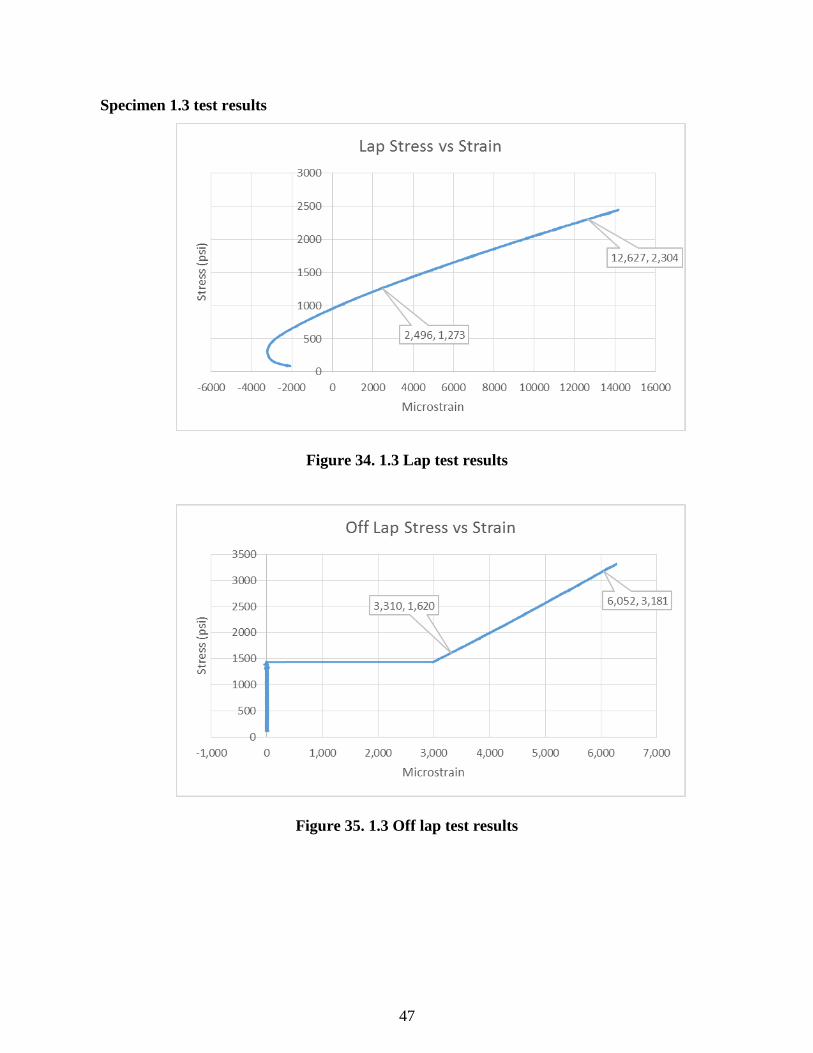
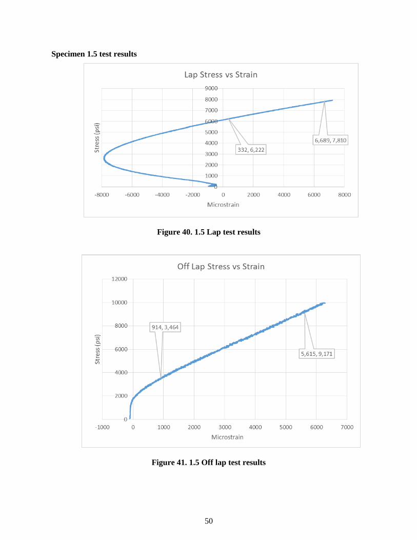
The tensile moduli listed in Table 6 were calculated for each specimen using the graphs
below. The tensile modulus is the slope between the two points shown on the graph.
Specimen 0.2A
Figure 25. 0.2A lap test result

43
Figure 26. 0.2A off lap test result
Figure 27. 0.2A Back side test results

44
Specimen 0.3A
Figure 28. 0.3A Lap test results
Figure 29. 0.3A off lap test results

45
Figure 30. 0.3A Back side test results
Specimen 0.4A
Figure 31. 0.4A Lap results

46
Figure 32. 0.4A Off lap test results
Figure 33. 0.4A Back side test results
47
Specimen 1.3 test results
Figure 34. 1.3 Lap test results
Figure 35. 1.3 Off lap test results

48
Figure 36. 1.3 Back side test results
Specimen 1.4 test results
Figure 37. 1.4 Lap test results

49
Figure 38. 1.4 Off lap test results
Figure 39. 1.4 Back side test results
50
Specimen 1.5 test results
Figure 40. 1.5 Lap test results
Figure 41. 1.5 Off lap test results

51
Figure 42. 1.5 Back side test results
Specimen 1.6 test results
Figure 43. 1.6 Lap test results

52
Figure 44. 1.6 Off lap test results
Figure 45. 1.6 Back side test results

53
Specimen 2.1 test results
Figure 46. 2.1 Lap test results
Figure 47. 2.1 Off lap test results

54
Figure 48. 2.1 Back side test results
Specimen 2.2 test results
Figure 49. 2.2 Lap test results
55
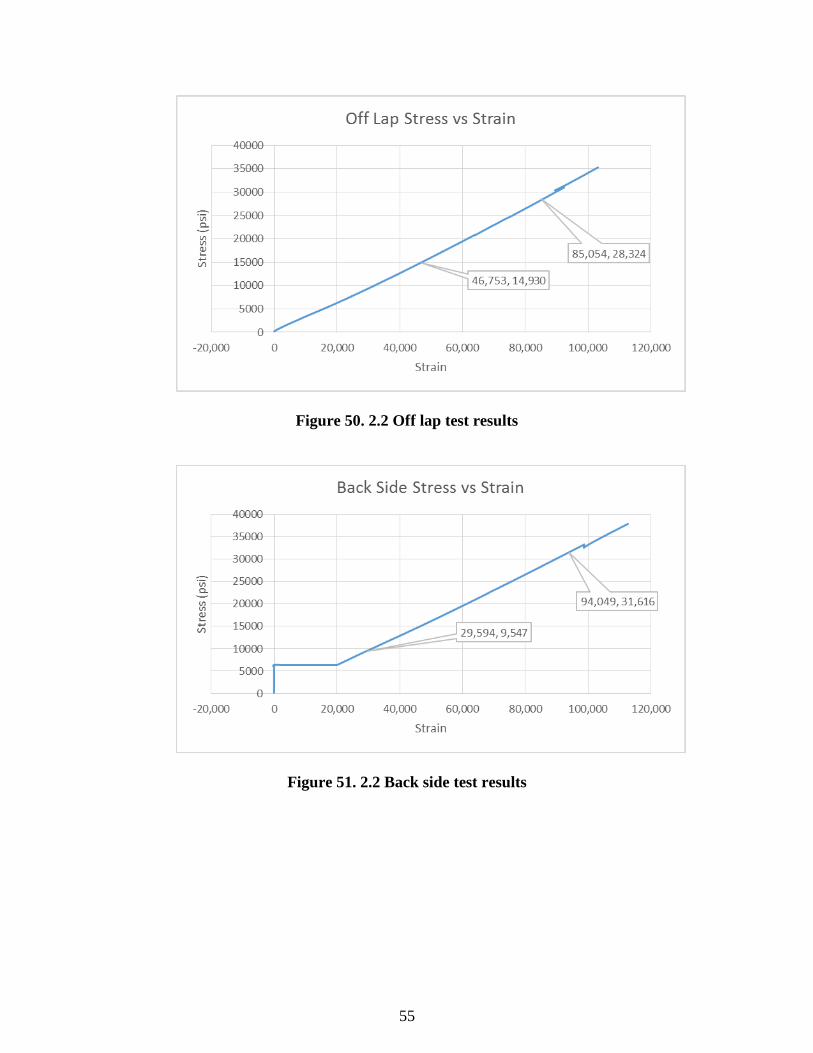
Figure 50. 2.2 Off lap test results
Figure 51. 2.2 Back side test results
56
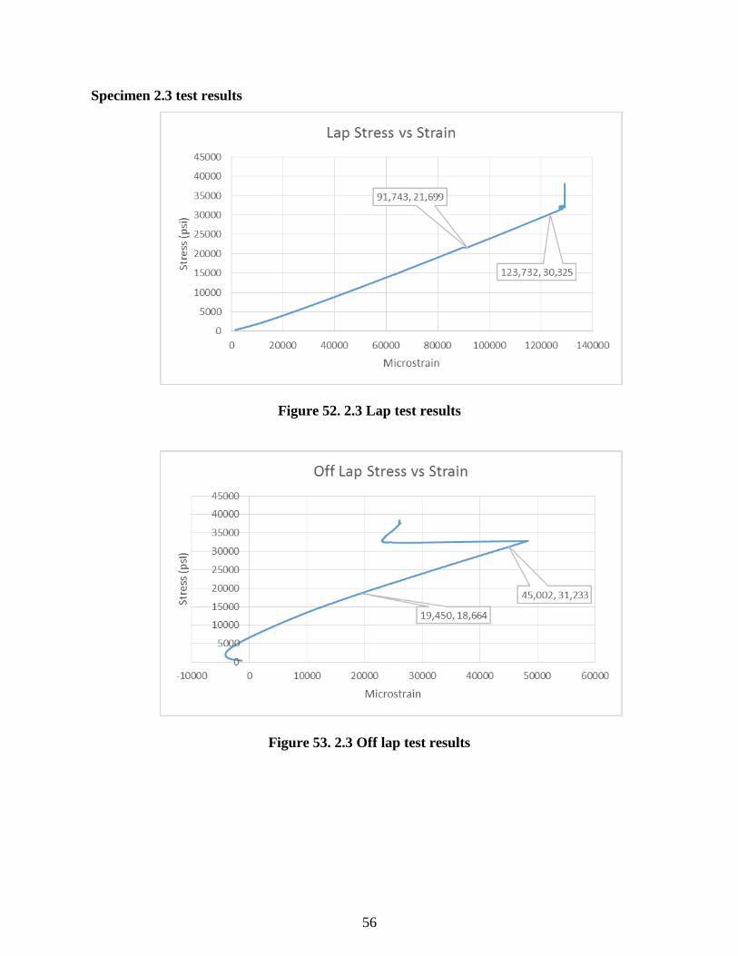
Specimen 2.3 test results
Figure 52. 2.3 Lap test results
Figure 53. 2.3 Off lap test results
57
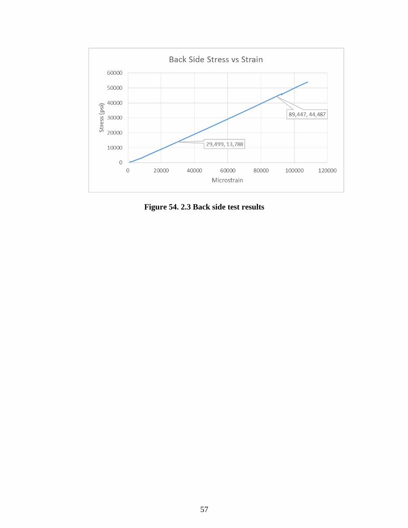
Figure 54. 2.3 Back side test results

58
Appendix B - Modified Volkersen Model Results
The equations shown below were used to determine the shear stress distribution
according to the modified Volkersen model for each specimen. The shear stress distribution was
then used to determine the actual stiffness and average stiffness of the lap joint.
Figure 55. Equations used in modified Volkersen model
Volkersen 1-Dimensional Shear Lag model
𝜏 𝑥 = 𝜆𝑃𝑥
𝑛−𝐶0
𝜆2
( 𝜆𝑥)
(𝜆𝑐)+𝑃𝑥
𝑛
(𝜆𝑥)
(𝜆𝑐)
𝜆2 =𝐺𝑎𝑡𝑎
1
𝐸𝑜𝑡𝑜+
1
𝐸𝑖(𝑛 − 1)𝑡𝑖
𝐶0 =𝐺𝑎𝑃𝑥
𝐸𝑖 (𝑛 − 1)𝑡𝑖 𝑡𝑎
Assumptions:1. Constant bond and adherend thickness.2. Uniform distribution of shear strain through the adhesive thickness.3. Adhesive carries only out-of-plane stresses while adherends carry only in-plane stresses.4.Linear elastic material behavior.5. Deformation of the adherends in the out-of-plane direction is negligible.
Overlap length = 2cPx = Applied forceEo = Modulus of elasticity of outer adherend, ksiEi = Modulus of elasticity of inner adherend, ksito = thickness of outer adherend, in.ti = thickness of inner adherend, in.ta = thcikness of adhesive, in.Ga = Shear modulus of adhesive, ksin = Total number of layers at lap
𝐺𝑎 =𝐸𝑎
1+ 𝑚
59
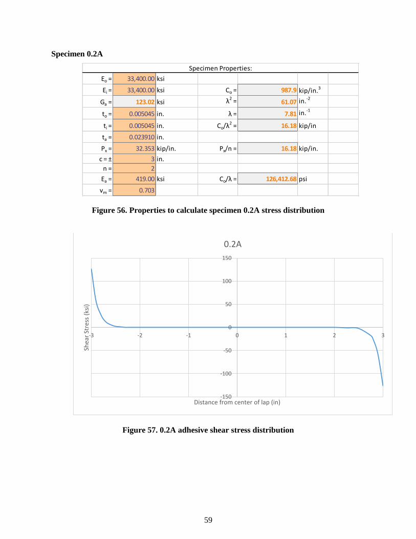
Specimen 0.2A
Figure 56. Properties to calculate specimen 0.2A stress distribution
Figure 57. 0.2A adhesive shear stress distribution
Eo = 33,400.00 ksi
Ei = 33,400.00 ksi Co = 987.9 kip/in.3
Ga = 123.02 ksi λ2 = 61.07 in.-2
to = 0.005045 in. λ = 7.81 in.-1
ti = 0.005045 in. Co/λ2 = 16.18 kip/in
ta = 0.023910 in.
Px = 32.353 kip/in. Px/n = 16.18 kip/in.
c = ± 3 in.
n = 2
Ea = 419.00 ksi Co/λ = 126,412.68 psi
vm = 0.703
Specimen Properties:
-150
-100
-50
0
50
100
150
-3 -2 -1 0 1 2 3
Shea
r St
ress
(ks
i)
Distance from center of lap (in)
0.2A

60
Figure 58. 0.2A joint stiffness
Specimen 0.3 A
Figure 59. Properties to calculate specimen 0.3A stress distribution
9,724
8,320
0
2000
4000
6000
8000
10000
12000
-4 -3 -2 -1 0 1 2 3 4
Stif
fnes
s (l
b/i
n)
Distance from center of lap (in)
0.2A Average Stiffness
Actual Stiffness
Average Stiffness
Eo = 33,400.00 ksi
Ei = 33,400.00 ksi Co = 400.6 kip/in.3
Ga = 115.11 ksi λ2 = 29.76 in.-2
to = 0.005045 in. λ = 5.46 in.-1
ti = 0.005045 in. Co/λ2 = 13.46 kip/in
ta = 0.045910 in.
Px = 26.923 kip/in. Px/n = 13.46 kip/in.
c = ± 3 in.
n = 2
Ea = 419.00 ksi Co/λ = 73,435.71 psi
vm = 0.82
Specimen Properties:
61
Figure 60. 0.3A adhesive shear stress distribution
Figure 61. 0.3A joint stiffness
-100
-80
-60
-40
-20
0
20
40
60
80
100
-3 -2 -1 0 1 2 3
Shea
r St
ress
(ks
i)
Distance from center of lap (in)
0.3A
6,111
5,296
0
1000
2000
3000
4000
5000
6000
7000
-4 -3 -2 -1 0 1 2 3 4
Stif
fnes
s (l
b/i
n)
Distance from center of lap (in)
0.3A Stiffness
Actual Stiffness
Average Stiffness
62
Specimen 0.4A
Figure 62. Properties to calculate specimen 0.4A stress distribution
Figure 63. 0.4A adhesive shear stress distribution
Eo = 33,400.00 ksi
Ei = 33,400.00 ksi Co = 483.6 kip/in.3
Ga = 118.29 ksi λ2 = 41.41 in.-2
to = 0.005045 in. λ = 6.43 in.-1
ti = 0.005045 in. Co/λ2 = 11.68 kip/in
ta = 0.033910 in.
Px = 23.358 kip/in. Px/n = 11.68 kip/in.
c = ± 3 in.
n = 2
Ea = 419.00 ksi Co/λ = 75,151.16 psi
vm = 0.771
Specimen Properties:
-100
-80
-60
-40
-20
0
20
40
60
80
100
-3 -2 -1 0 1 2 3
Shea
r St
ress
(ks
i)
Distance from center of lap (in)
0.4A

63
Figure 64. 0.4A joint stiffness
Specimen 1.3
Figure 65. Properties to calculate specimen 1.3 stress distribution
6,260
5,425
0
1000
2000
3000
4000
5000
6000
7000
-4 -3 -2 -1 0 1 2 3 4
Stif
fnes
s (l
b/i
n)
Distance from center of lap (in)
0.4A Stiffness
Actual Stiffness
Average Stiffness
Eo = 33,400.00 ksi
Ei = 33,400.00 ksi Co = 15.3 kip/in.3
Ga = 113.06 ksi λ2 = 21.67 in.-2
to = 0.005045 in. λ = 4.65 in.-1
ti = 0.005045 in. Co/λ2 = 0.71 kip/in
ta = 0.046455 in.
Px = 2.121 kip/in. Px/n = 0.71 kip/in.
c = ± 3 in.
n = 3
Ea = 419.00 ksi Co/λ = 3,290.78 psi
vm = 0.853
Specimen Properties:

64
Figure 66. 1.3 adhesive shear stress distribution
Figure 67. 1.3 joint stiffness
-4
-3
-2
-1
0
1
2
3
4
-3 -2 -1 0 1 2 3
Shea
r St
ress
(ks
i)
Distance from center of lap (in)
1.3
273
237
0
50
100
150
200
250
300
-4 -3 -2 -1 0 1 2 3 4
Stif
fnes
s (l
b/i
n)
Distance from center of lap (in)
1.3 Stiffness
Actual Stiffness
Average Stiffness
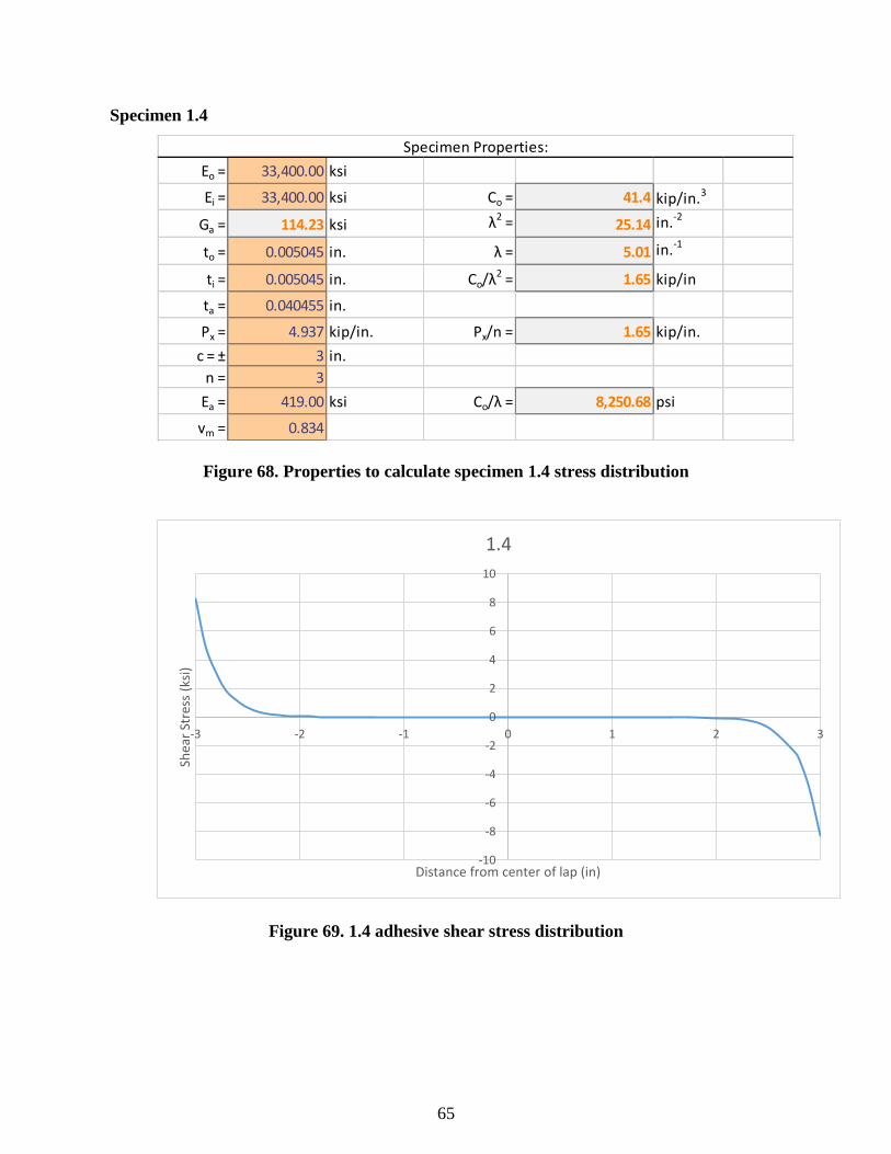
65
Specimen 1.4
Figure 68. Properties to calculate specimen 1.4 stress distribution
Figure 69. 1.4 adhesive shear stress distribution
Eo = 33,400.00 ksi
Ei = 33,400.00 ksi Co = 41.4 kip/in.3
Ga = 114.23 ksi λ2 = 25.14 in.-2
to = 0.005045 in. λ = 5.01 in.-1
ti = 0.005045 in. Co/λ2 = 1.65 kip/in
ta = 0.040455 in.
Px = 4.937 kip/in. Px/n = 1.65 kip/in.
c = ± 3 in.
n = 3
Ea = 419.00 ksi Co/λ = 8,250.68 psi
vm = 0.834
Specimen Properties:
-10
-8
-6
-4
-2
0
2
4
6
8
10
-3 -2 -1 0 1 2 3
Shea
r St
ress
(ks
i)
Distance from center of lap (in)
1.4

66
Figure 70. 1.4 joint stiffness
Specimen 1.5
Figure 71. Properties to calculate specimen 1.5 stress distribution
686
595
0
100
200
300
400
500
600
700
800
-4 -3 -2 -1 0 1 2 3 4
Stif
fnes
s (l
b/i
n)
Distance from center of lap (in)
1.4 Stiffness
Actual Stiffness
Average Stiffness
Eo = 33,400.00 ksi
Ei = 33,400.00 ksi Co = 52.1 kip/in.3
Ga = 114.17 ksi λ2 = 24.82 in.-2
to = 0.005045 in. λ = 4.98 in.-1
ti = 0.005045 in. Co/λ2 = 2.10 kip/in
ta = 0.040955 in.
Px = 6.3 kip/in. Px/n = 2.10 kip/in.
c = ± 3 in.
n = 3
Ea = 419.00 ksi Co/λ = 10,461.20 psi
vm = 0.835
Specimen Properties:

67
Figure 72. 1.5 adhesive shear stress distribution
Figure 73. 1.5 joint stiffness
-15
-10
-5
0
5
10
15
-3 -2 -1 0 1 2 3
Shea
r St
ress
(ks
i)
Distance from center of lap (in)
1.5
870
754
0
100
200
300
400
500
600
700
800
900
1000
-4 -3 -2 -1 0 1 2 3 4
Stif
fnes
s (l
b/i
n)
Distance from center of lap (in)
1.5 Stiffness
Actual Stiffness
Average Stiffness

68
Specimen 1.6
Figure 74. Properties to calculate specimen 1.6 stress distribution
Figure 75. 1.6 adhesive shear stress distribution
Eo = 33,400.00 ksi
Ei = 33,400.00 ksi Co = 61.0 kip/in.3
Ga = 116.32 ksi λ2 = 31.42 in.-2
to = 0.005045 in. λ = 5.61 in.-1
ti = 0.005045 in. Co/λ2 = 1.94 kip/in
ta = 0.032955 in.
Px = 5.823 kip/in. Px/n = 1.94 kip/in.
c = ± 3 in.
n = 3
Ea = 419.00 ksi Co/λ = 10,880.32 psi
vm = 0.801
Specimen Properties:
-15
-10
-5
0
5
10
15
-3 -2 -1 0 1 2 3
Shea
r St
ress
(ks
i)
Distance from center of lap (in)
1.6

69
Figure 76. 1.6 joint stiffness
Specimen 2.1
Figure 77. Properties to calculate specimen 2.1 stress distribution
906
785
0
100
200
300
400
500
600
700
800
900
1000
-4 -3 -2 -1 0 1 2 3 4
Stif
fnes
s (l
b/i
n)
Distance from center of lap (in)
1.6 Stiffness
Actual Stiffness
Average Stiffness
Eo = 33,400.00 ksi
Ei = 33,400.00 ksi Co = 239.5 kip/in.3
Ga = 114.29 ksi λ2 = 24.46 in.-2
to = 0.005045 in. λ = 4.95 in.-1
ti = 0.005045 in. Co/λ2 = 9.79 kip/in
ta = 0.036970 in.
Px = 39.169 kip/in. Px/n = 9.79 kip/in.
c = ± 3 in.
n = 4
Ea = 419.00 ksi Co/λ = 48,432.19 psi
vm = 0.833
Specimen Properties:
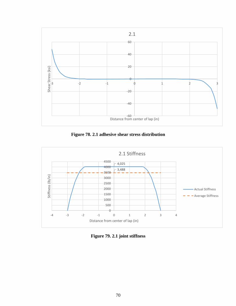
70
Figure 78. 2.1 adhesive shear stress distribution
Figure 79. 2.1 joint stiffness
-60
-40
-20
0
20
40
60
-3 -2 -1 0 1 2 3
Shea
r St
ress
(ks
i)
Distance from center of lap (in)
2.1
4,025
3,488
0
500
1000
1500
2000
2500
3000
3500
4000
4500
-4 -3 -2 -1 0 1 2 3 4
Stif
fnes
s (l
b/i
n)
Distance from center of lap (in)
2.1 Stiffness
Actual Stiffness
Average Stiffness
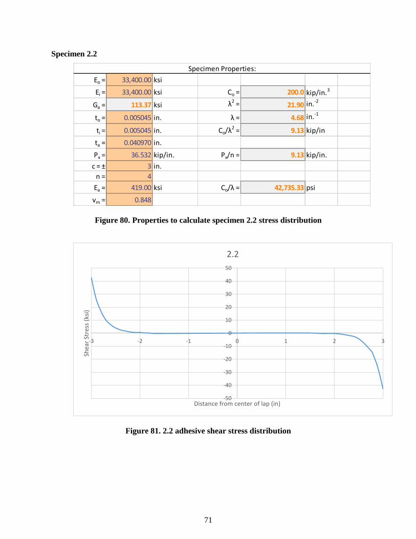
71
Specimen 2.2
Figure 80. Properties to calculate specimen 2.2 stress distribution
Figure 81. 2.2 adhesive shear stress distribution
Eo = 33,400.00 ksi
Ei = 33,400.00 ksi Co = 200.0 kip/in.3
Ga = 113.37 ksi λ2 = 21.90 in.-2
to = 0.005045 in. λ = 4.68 in.-1
ti = 0.005045 in. Co/λ2 = 9.13 kip/in
ta = 0.040970 in.
Px = 36.532 kip/in. Px/n = 9.13 kip/in.
c = ± 3 in.
n = 4
Ea = 419.00 ksi Co/λ = 42,735.33 psi
vm = 0.848
Specimen Properties:
-50
-40
-30
-20
-10
0
10
20
30
40
50
-3 -2 -1 0 1 2 3
Shea
r St
ress
(ks
i)
Distance from center of lap (in)
2.2

72
Figure 82. 2.2 joint stiffness
Specimen 2.3
Figure 83. Properties to calculate specimen 2.3 stress distribution
3,548
3,154
0
500
1000
1500
2000
2500
3000
3500
4000
-4 -3 -2 -1 0 1 2 3 4
Stif
fnes
s (l
b/i
n)
Distance from center of lap (in)
2.2 Stiffness
Actual Stiffness
Average Stiffness
Eo = 33,400.00 ksi
Ei = 33,400.00 ksi Co = 154.7 kip/in.3
Ga = 113.43 ksi λ2 = 22.09 in.-2
to = 0.005045 in. λ = 4.70 in.-1
ti = 0.005045 in. Co/λ2 = 7.01 kip/in
ta = 0.040637 in.
Px = 28.02 kip/in. Px/n = 7.01 kip/in.
c = ± 3 in.
n = 4
Ea = 419.00 ksi Co/λ = 32,920.88 psi
vm = 0.847
Specimen Properties:

73
Figure 84. 2.3 adhesive shear stress distribution
Figure 85. 2.3 joint stiffness
-40
-30
-20
-10
0
10
20
30
40
-3 -2 -1 0 1 2 3
Shea
r St
ress
(ks
i)
Distance from center of lap (in)
2.3
2,734
2,369
0
500
1000
1500
2000
2500
3000
-4 -3 -2 -1 0 1 2 3 4
Stif
fnes
s (l
b/i
n)
Distance from center of lap (in)
2.3 Stiffness
Actual Stiffness
Average Stiffness