011-0370

Research on Optimization of Hub-And-Spoke Logistics Network Design with

Impedance Effect

Sun Li, Zhao Lindu*

Institute of Systems Engineering, Southeast University

Nanjing, Jiangsu, 210096, China

*Corresponding author. ldzhao@seu.edu.cn, +86-25-52090759

sunsuper@126.com

POMS 20th Annual Conference

Orlando, Florida, U.S.A

May 1 to May 4, 2009

RESEARCH ON OPTIMIZATION OF HUB-AND-SPOKE LOGISTICS

NETWORK DESIGN WITH IMPEDANCE EFFECT

LI SUN, LINDU ZHAO

Institute of Systems Engineering

Southeast University

Nanjing, Jiangsu, P.R. China, 210096

Email: sunsuper@126.com, ldzhao@seu.edu.cn

Abstract: Hub-and-spoke pattern is one of the most important forms of modern

logistics network. In order to treat with the capacitated single allocation p-hub

problem, this paper presents a new non-linear programming model to design the

network. Due to the fact that the current researches have some limitations, the

capacity of materials disposal at hubs and the capacity limit of courses between hubs

are treated as constraints in the model based on the analysis of characteristics of

hub-and-spoke logistics network. In the process of optimization, an impedance

function is introduced to balance some local logistics quantity properly in order to

avoid congestions. Additionally, we provide a genetic algorithm that finds

high-quality solutions within reasonable time. Then an example and simulation is

given to verify the validity of the model. The results of the model provide new and

realistic insights into the hub-and-spoke network design problem.

Keywords: Hub-and-spoke network design; Impedance function; Non-linear

programming; Genetic algorithm

1. Introduction. With the rapid development of the global economy, the huge

economic value of logistics, which is treated as “the third spring of profit”, is

appearing gradually. Because of this, logistics draws more and more attention of

governments and enterprises. For many years, logistics has been one of the hottest

issues which are concerned by academe. The research results of various problems in

the field of logistics emerge in endlessly. Among the issues, the hub-and-spoke

network is a special construction of logistics networks. It plays an important effect in

practical production and life. It is also one of the current research objects of academe.

With the development of logistics industry, the scale of logistics networks is

extending all the time. The traditional logistics pattern, such as “one-to-one” and

“many-to-many”, can not cover a wide area effectively because of the factors of costs,

time limit and so on. So they can not construct a wide spoke network of logistics.

Therefore, the multi-level logistics pattern, which is represented by LD-LED model,

has become the trend of the development of logistics system. The hub-and-spoke

logistics network is one of the manifestations of LD-LED model [1]. Its appearance is

due to the enterprises’ pursuits for scale economic benefits [2]. The hub-and-spoke

logistics network collects a great deal of dispersed point-to-point logistics operations

to few hub nodes and main stems by some spoke nodes in order to utilize the

advantages of the hub nodes’ ability of materials disposal and main stems’

transportation. By this way, a certain degree of scale economic benefits can be

obtained. The redundancy costs and wastages of the system can be reduced. So the

operation efficiency of the whole logistics network can be improved. This pattern of

logistics network is widely used in the airline industry, telecommunications [3] and

postal delivery systems.

A typical hub-and-spoke network is composed by plentiful demand nodes and a

certain number of hub nodes which have transfer function. There are a certain number

of materials flows between each pair of demand nodes. The materials flows must

route all their traffic from origin nodes to destination nodes indirectly via one or more

hubs. There are no direct connects between any demand nodes. The operation costs of

whole of the hub-and-spoke logistics network are made up of the distances between

nodes and the expenses of transportations of materials.

Because of its wide usage, the hub-and-spoke network is worthy studying. Many

home and broad scholars have many researches in the field. O’Kelly [4] developed a

quadratic programming model and proposed two enumeration heuristics. Campbell [5]

presented integer programming formulations for four types of discrete hub location

problems. He also introduced discrete hub center and hub covering problems, basic

formulations and formulations with flow thresholds for spokes. Ernst and

Krishnamoorthy [6] considered that each non-hub node may be allocated to multiple

hubs rather than sending and receiving all of its flow to and from a single hub. They

presented a new MILP formulation for the multiple allocation p-hub median problems.

Matsubayashi [7] studied a cost allocation problem arising from hub–spoke network

systems and formulated this problem as a cooperative game and analyze the core

allocation, which was a widely used solution concept. Elhedhli and Hu [8] considered

a hub-and-spoke network design problem with congestion. They proposed a model

extending current models by taking congestion effects into account, which was

achieved through a non-linear cost term in the objective function. Lin and Chen [9]

proposed a generalized hub-and-spoke network in a capacitated and directed network

configuration that integrated the operations of three common hub-and-spoke networks:

pure, stopover and center directs. Klincewica[10] described an algorithm, based on

dual ascent and dual adjustment techniques within a branch-and-bound scheme, for

the uncapacitated hub location problem (UHLP). Jeong [11] addressed a

hub-and-spoke network problem for railroad freight, where a central planner was to

find transport routes, frequency of service, length of trains to be used, and

transportation quantity.

The most current researches on optimization of hub-and-spoke network

concentrate at the uncapacitated hubs allocation problem. However, in the actual

process of logistics, each hub node has a certain capacity of materials transfer. This

makes each hub node can only dispose finite materials in a certain time segment. If

the limitation of capacity of hub nodes is neglected in the optimization model, the

applicability of the model will be influenced in a certain degree. From the perspective

of the transportation system, the carrying capacity of a road is one of the most

important elements. It influences the result of optimization in a certain degree. In the

field of logistics planning, it can be interpreted as the materials capacity of a section.

When the materials quantity on a section is bigger than its capacity, congestion will be

caused and even paralysis of the logistics network will happen. In addition, most of

current researches focus on the goal of reducing the building and the operation costs

of a logistics network. The caused result is that they paid much attention on

improving economic benefits of the logistics network itself while neglecting the

possible reduction of the performance of the network caused in the process of pursuits

for economic benefits. It should be known that a hub-and-spoke logistics network

built on the goal of lowest costs may in a certain degree has some hidden troubles of

paralysis caused by too much local materials. Therefore, this paper adds the

constraints of hub nodes’ capacity of materials disposal and sections’ capacity of

materials in the new optimization model. Besides, we also try to balance some local

materials quantity in order to improve the whole performance of a logistics network.

So we can increase the whole stability of the network while optimizing the operation

costs of the network. We treat the operation costs as two parts: building costs and

congestion costs. Elhedhli [8] managed to balance the materials quantity by adding

congestion costs in the objective function. But we try to use the section impedance

function in the theory of transportation as the congestion costs function. Because the

building costs and the congestion costs have different dimensions, we build a

multi-objective model to solve the problem.

The paper is structured as follows. In the next section we provide the description

of the hub-and-spoke logistics network optimization problem. In Section 3 we present

our new nonlinear multi-objective programming model. In Section 4 we design a

genetic algorithm to solve this model. We also give an example and simulation of the

model in Section 5. Finally we make some concluding remarks in Section 6.

2. Description of hub-and-spoke network optimization problem. For a common

hub-and-spoke network G(V, A), the set of demand nodes is N and the set of hub

nodes is M. M∪ N=V, M∩ N=∅ . There is a certain materials quantity between each

demand node pair. Any demand node can be the original node of a material flow and

it can also be the destination node. When a material flow will be delivered between a

pair of demand nodes, after leaving from the original node, it must arrive at the

corresponding destination node via one or more hub nodes. There are no logistics

flows between demand nodes directly. In a common sense, the functions of a hub

node are collection, sorting and transfer. The materials coming from multiple origins

are collected and sorted in term of their different destinations at a hub node. Then the

materials which have the same destination orientation are combined and transported

by transportation tools which have better transportation ability through main stems.

After arriving at the target hub node, the combined materials will be sorted again in

term of their final targets and then be sent to the destination nodes respectively. Take

the postal logistics network for example. The postal logistics network is a typical

hub-and-spoke network. The demand nodes are equal to the small areas’ post offices

and the hub nodes are equal to large areas’ sorting offices. After collecting a certain

number of mails which come from dispersed customers and fixed mail boxes, a post

office delivers the mails to the large area’s sorting office which it belongs to. The

sorting office classifies the mails in term of their destination addresses and the

congener mails are collected and sent to the corresponding large area’s sorting office

through fixed route. Based on the detail of destination addresses, the mails are sorted

at sorting office again and are delivered to the destinations eventually. The structure

of a typical hub-and-spoke network is shown in Figure 1.

FIGURE 1. Structure of a hub-and-spoke network

There are a lot of research orientations about the optimization of the

hub-and-spoke network. This paper mainly focuses on the optimization problem of

the logistics routes between demand nodes where the demand nodes and hub nodes

are already provided. Given the set of demand nodes N and the set of hub nodes M,

we try to allocate p proper hub nodes k1, k2, …, kp∈M for each pair of demand node

(i, j), i, j∈N in order to implement the transfer of the materials and optimize the

performance of the whole logistics network. For increasing the practicality of the

model, we consider the influences on the optimization result caused by the capacity of

materials disposal at hub nodes and the time limit of logistics. It should be pointed out

that optimizing the performance of logistics network dose not mean to only pursue the

lowest operation costs. It is necessary to ensure a certain degree of stability of

network for improving the service level of a logistics system. A logistics network

which often be congested and can not transport swimmingly will not satisfy

customers’ basic demands even its operation costs are lowest. Most of the former

researches’ goals are obtaining the lowest costs. The optimization results always make

some individual routes which have “better” transportation conditions take on huge

amount materials quantity. Obviously, the more materials taken on, the more likely

congestion and paralysis will happen in the section. This goes against ensuring the

stability of the logistic network. Therefore, it is needed to balance some materials

quantity properly. But it will increase logistics costs. It is clearly that the stability of a

logistics network and the logistics costs are contradicted. This paper tries to present a

method to balance the pair of the two contradicted factors.

3. Parameters configuration and model building. This paper proposes a nonlinear

multi-objective 0-1 programming model in order to realize the optimization of the

hub-and-spoke network’s performance.

As the above paragraph expatiates, we assume that N is the set of n demand nodes,

i, j∈N. M is the set of m candidate hub nodes and H is the set of hub nodes, H ⊂ M, k,

l∈H. p is the number of hub nodes. Let dik is the distance between demand node i and

hub node k as well as dkl is the distance between hub node k and l. Wij is the materials

quantity to be transported from demand node i to demand node j. Considering the

actual situation, Wij is not required to equal to Wji. Fk is the disposal and transfer

capacity of materials at hub node k. Xijkl is the decision variable representing whether

the route of i-k-l-j is selected. If a materials flow Wij starts from demand node i and

ends at demand node j, via hub node k and j by order, the route of i-k-l-j is selected

and Xijkl is 1. If else, Xijkl is 0.

The model is built under the following assumptions:

(1) Each materials flow must be transported via one or two hub nodes from its

origin node to destination node. For the decision variability Xijkl, k=l is allowed. It

represents that materials flow Wij starting from origin node i can be transported to

destination node j directly via hub node k;

(2) There must be one route between each pair of demand nodes (i, j) and the

route is unique;

(3) A demand node is allowed to be connected with multiple hub nodes. The

former constraint that a demand node must be connected with one hub node is

removed;

(4) Due to that the materials on the sections between demand nodes and hub

nodes are rather small, we consider that these sections will not be congested. The

section paralysis could only happen on the main stems between hub nodes because of

their huge materials quantity.

It is obvious that the more times for which a main stem is chosen, the more

frequent the cargo movements on it will be. Due to this it will be easier that

congestion and even paralysis happen on the main stem. So it is necessary to describe

the relationship between materials quantity and congestion degree on a section

quantitatively. In this paper, we use typical impedance function, Davidson function.

The function is as follows:

0( ) {1 [ / ( )]}a a a a a ac x c J x R x= + − (1)

In the above formulation, ca0 is the impedance on section a when there is no traffic

flow (min); xa is the traffic flow on section a (unit per day); Ka is the capacity of

section a (unit per day); J is a parameter of the model which is related to characterizes

of the section. The curve of the function is shown in Figure 2.

Ka flow

time

t0

FIGURE 2. Curve of Davidson function

As Figure 2 shows, the delay time increases with the traffic flow. When traffic

flow tends to the capacity of the section, delay time increases rapidly. In order to

avoid rapid increase of delay time, we should keep the traffic flow at a low level. In

this paper, we set the research object to be materials flow but not vehicle flow. So we

can get:

kl ijkl iji N j N

x X W∈ ∈

= ∑∑ (2)

Then we can change formulation (1) as follows:

0 0 0( ) {1 [ / ( )]} [ / ( ) 1]kl kl kl kl kl kl kl kl kl kl ijkl iji N j N

c x c J x R x c c J R R X W∈ ∈

= + − = + − −∑∑ (3)

Based on the above research, we build a nonlinear multi-objective 0-1

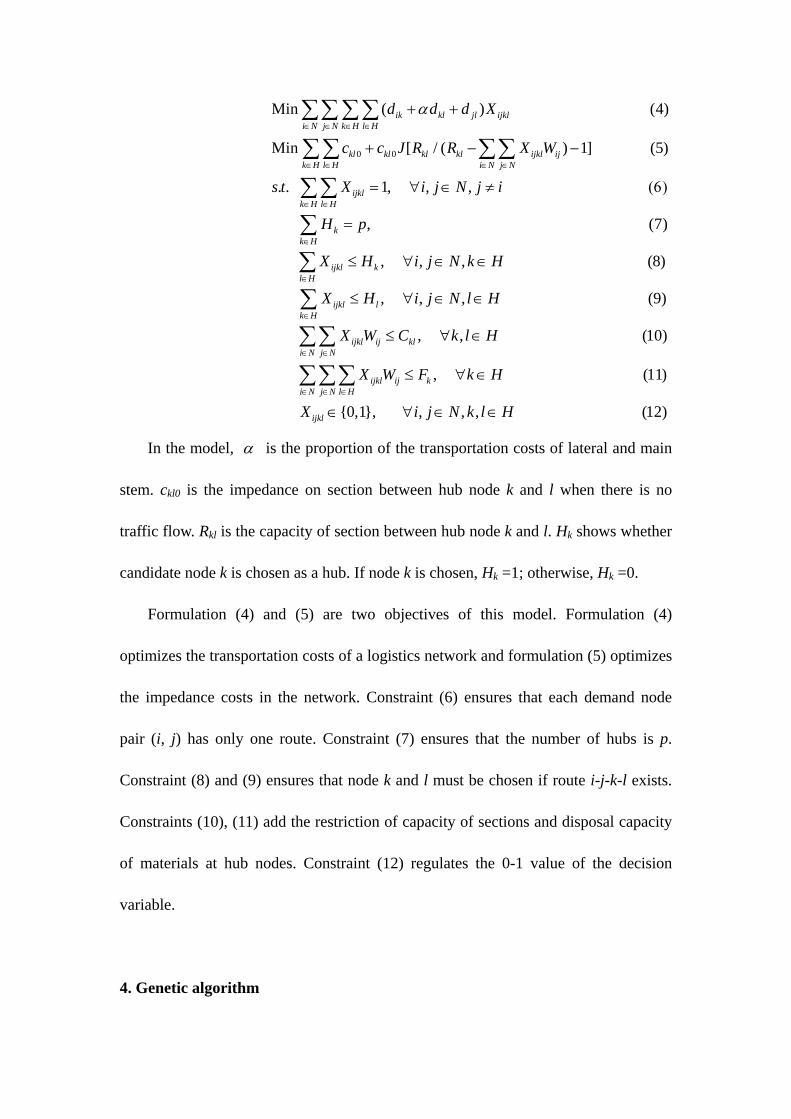
programming model which is shown as follows:

0 0

Min ( ) (4)

Min [ / ( ) 1] (5)

. . 1, , ,

ik kl jl ijkli N j N k H l H

kl kl kl kl ijkl ijk H l H i N j N

ijklk H l H

d d d X

c c J R R X W

s t X i j N j i

α∈ ∈ ∈ ∈

∈ ∈ ∈ ∈

∈ ∈

+ +

+ − −

= ∀ ∈ ≠

∑∑ ∑ ∑

∑ ∑ ∑∑

∑∑, (7)

, , , (8)

kk H

ijkl kl H

ijkl

H p

X H i j N k H

X

∈

∈

(6)

=

≤ ∀ ∈ ∈

∑

∑, , , (9)

, , (10)

,

lk H

ijkl ij kli N j N

ijkl ij ki N j N l H

H i j N l H

X W C k l H

X W F k H

∈

∈ ∈

∈ ∈ ∈

≤ ∀ ∈ ∈

≤ ∀ ∈

≤ ∀ ∈

∑

∑∑

∑∑∑ (11)

{0,1}, , , , (12)ijklX i j N k l H

∈ ∀ ∈ ∈

In the model, α is the proportion of the transportation costs of lateral and main

stem. ckl0 is the impedance on section between hub node k and l when there is no

traffic flow. Rkl is the capacity of section between hub node k and l. Hk shows whether

candidate node k is chosen as a hub. If node k is chosen, Hk =1; otherwise, Hk =0.

Formulation (4) and (5) are two objectives of this model. Formulation (4)

optimizes the transportation costs of a logistics network and formulation (5) optimizes

the impedance costs in the network. Constraint (6) ensures that each demand node

pair (i, j) has only one route. Constraint (7) ensures that the number of hubs is p.

Constraint (8) and (9) ensures that node k and l must be chosen if route i-j-k-l exists.

Constraints (10), (11) add the restriction of capacity of sections and disposal capacity

of materials at hub nodes. Constraint (12) regulates the 0-1 value of the decision

variable.

4. Genetic algorithm

For the model we built is non-linear, we develop a genetic algorithm to solve it.

The algorithm is described as follows.

Step 1: Select p nodes in M to form a new hub set H randomly;

Step 2: Generate the original population based on the coding rule;

Step 3: Estimate that whether every chromosome in the population satisfies the

constraints (10) and (11) in the model. If yes, turn to step 4. Otherwise, delete the

chromosome and generate a new one and repeat step 3;

Step 4: Using the fitness function to evaluate fitness value for every chromosome

in population;

Step 5: Calculate selection probability for each chromosome based on its fitness

value;

Step 6: Choose chromosomes prepared to be crossed using selection function;

Step 7: Cross the population using the custom crossover function;

Step 8: Mutate the population using the custom mutation function;

Step 9: If the number of iteration is enough, turn to step 10; otherwise, turn to step

4;

Step 10: Save the solution represented by the population. If there is possible H

which is different from formers, turn to step 1; Otherwise, over.

Some rules and functions referred in the above algorithm are expressed infra.

(1) Coding rule: Using a 2n2 dimension vector to as a chromosome. We select a

hub node in H randomly as the value for each element in the vector. In the vector, two

adjacent elements represent a route. Figure 3 gives a 2n2 vector. From left to right,

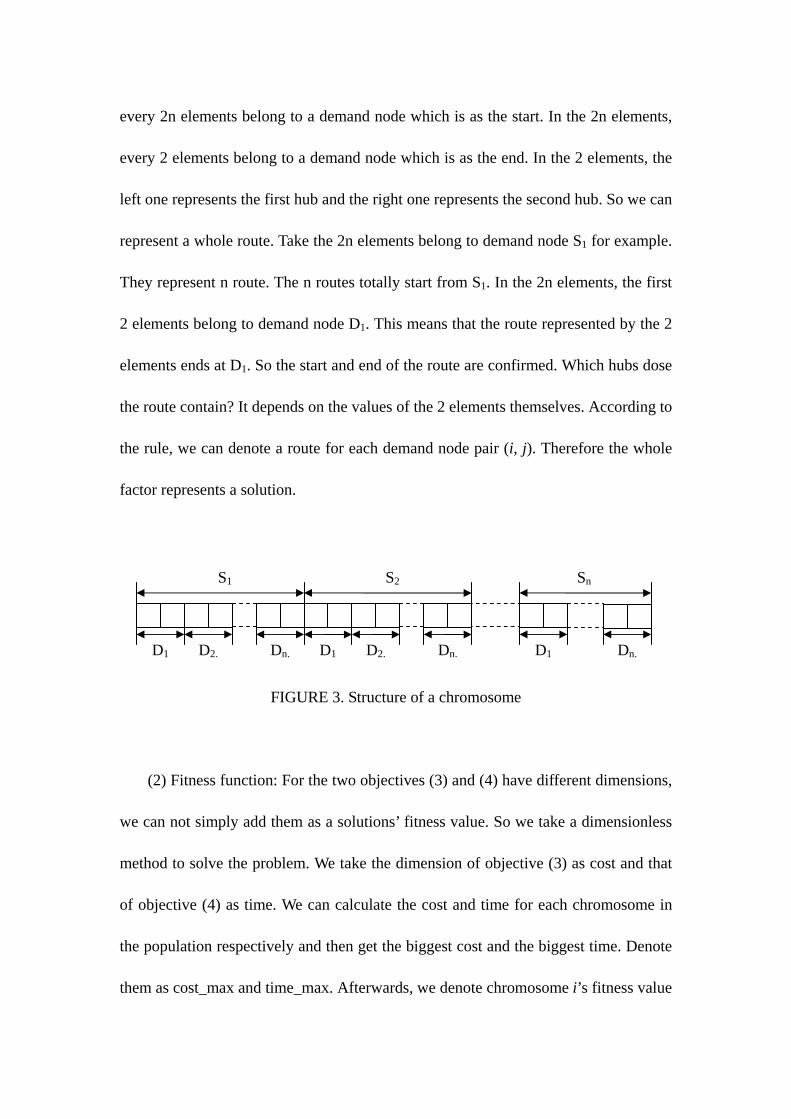
every 2n elements belong to a demand node which is as the start. In the 2n elements,

every 2 elements belong to a demand node which is as the end. In the 2 elements, the

left one represents the first hub and the right one represents the second hub. So we can

represent a whole route. Take the 2n elements belong to demand node S1 for example.

They represent n route. The n routes totally start from S1. In the 2n elements, the first

2 elements belong to demand node D1. This means that the route represented by the 2

elements ends at D1. So the start and end of the route are confirmed. Which hubs dose

the route contain? It depends on the values of the 2 elements themselves. According to

the rule, we can denote a route for each demand node pair (i, j). Therefore the whole

factor represents a solution.

FIGURE 3. Structure of a chromosome

(2) Fitness function: For the two objectives (3) and (4) have different dimensions,

we can not simply add them as a solutions’ fitness value. So we take a dimensionless

method to solve the problem. We take the dimension of objective (3) as cost and that

of objective (4) as time. We can calculate the cost and time for each chromosome in

the population respectively and then get the biggest cost and the biggest time. Denote

them as cost_max and time_max. Afterwards, we denote chromosome i’s fitness value

S1

D1 D2. Dn.

S2 Sn

D1 D2. Dn. Dn. D1

like this:

( ) cos ( ) / cos _ max ( ) / _ maxFitvalue i t i t time i time= + (13)

(3) Crossover function: In the population we select two chromosomes randomly.

Then choose a certain number of demand node pairs to exchange their routes. First,

find the elements representing the route between a node pairs in two chromosomes.

Second, exchange the values. Then we can obtain two new chromosomes. If the two

new chromosomes both satisfy constrains in the model, we select two chromosomes

with smallest fitness value in the 2 new chromosomes and 2 old chromosomes; If not,

repeat this operation. Figure 4 shows the process of crossover.

FIGURE 4. The process of crossover

(4) Mutation function: After a certain number of iterations, we choose a demand

node pair randomly and change the route of it by selecting hub nodes in H randomly.

Of course this operation must ensure the new chromosome satisfy constraints in the

model.

5. Example and simulations. In order to verify the validity of the model and the

i i+1 j j+1 k k+1

i i+1 j j+1 k k+1

algorithm we designed in the above paragraph, we give an example in this section. We

use Matlab 7.1 to do numerical simulation.

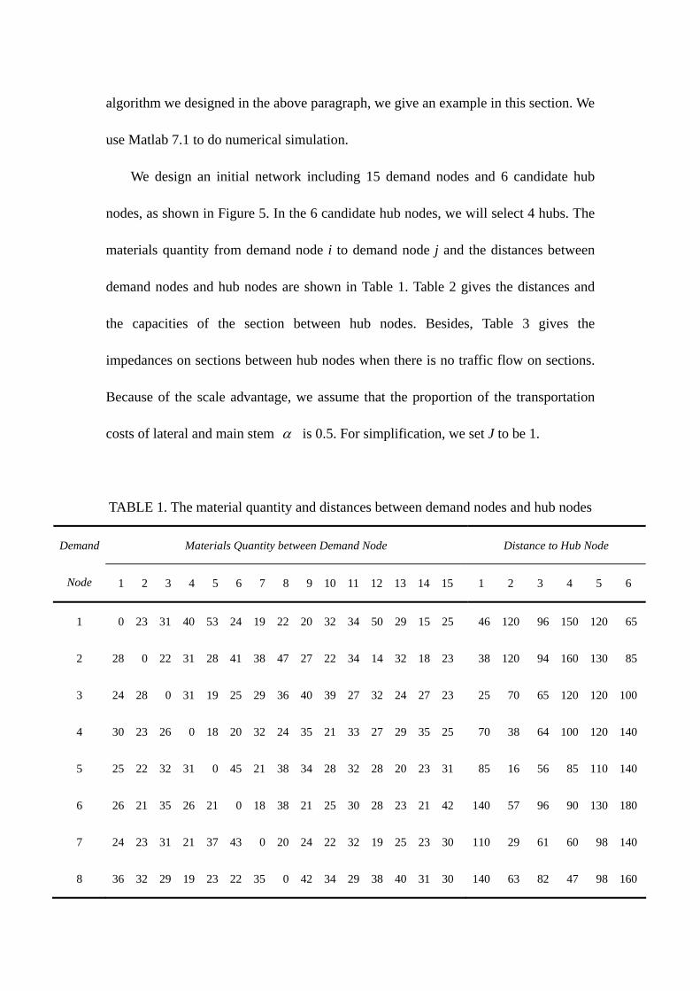
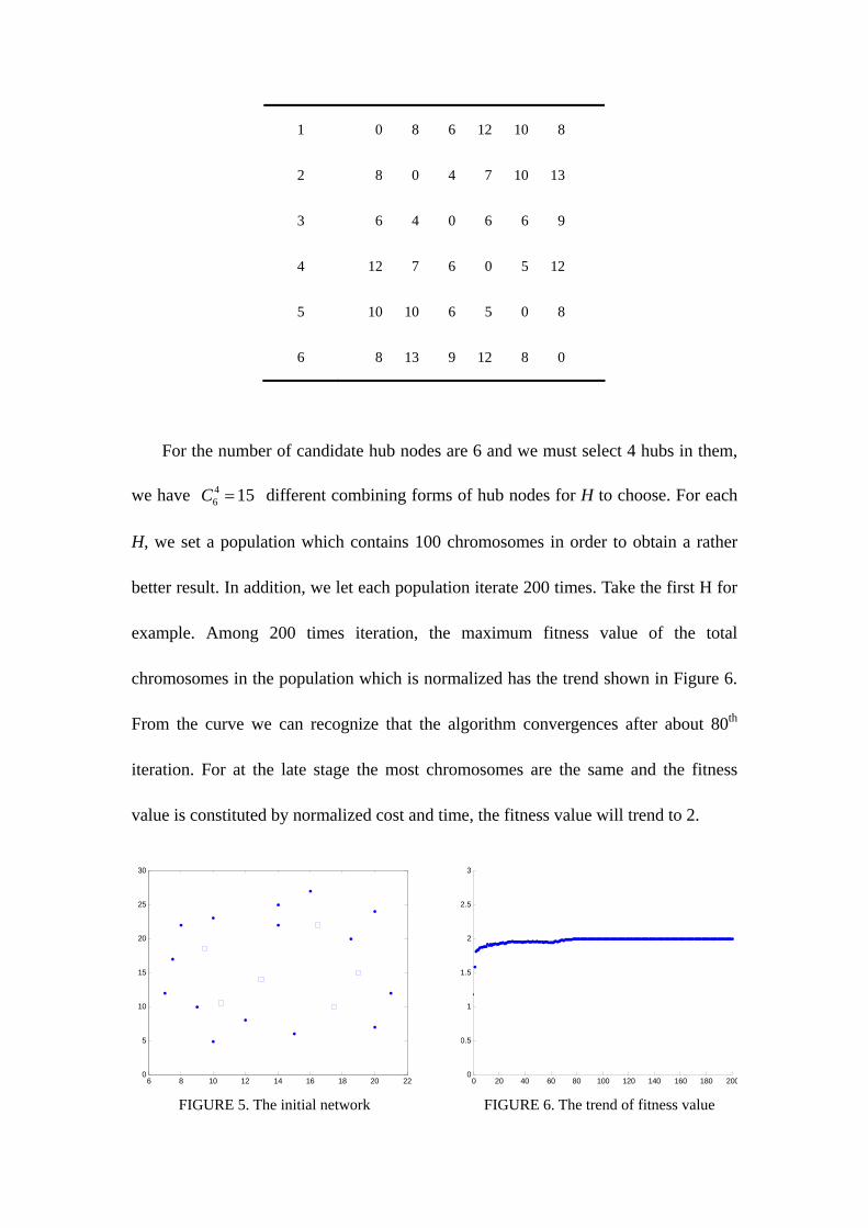
We design an initial network including 15 demand nodes and 6 candidate hub

nodes, as shown in Figure 5. In the 6 candidate hub nodes, we will select 4 hubs. The

materials quantity from demand node i to demand node j and the distances between

demand nodes and hub nodes are shown in Table 1. Table 2 gives the distances and

the capacities of the section between hub nodes. Besides, Table 3 gives the

impedances on sections between hub nodes when there is no traffic flow on sections.

Because of the scale advantage, we assume that the proportion of the transportation

costs of lateral and main stem α is 0.5. For simplification, we set J to be 1.

TABLE 1. The material quantity and distances between demand nodes and hub nodes

Materials Quantity between Demand Node Distance to Hub Node Demand

Node 1 2 3 4 5 6 7 8 9 10 11 12 13 14 15 1 2 3 4 5 6

1

2

3

4

5

6

7

8

0 23 31 40 53 24 19 22 20 32 34 50 29 15 25

28 0 22 31 28 41 38 47 27 22 34 14 32 18 23

24 28 0 31 19 25 29 36 40 39 27 32 24 27 23

30 23 26 0 18 20 32 24 35 21 33 27 29 35 25

25 22 32 31 0 45 21 38 34 28 32 28 20 23 31

26 21 35 26 21 0 18 38 21 25 30 28 23 21 42

24 23 31 21 37 43 0 20 24 22 32 19 25 23 30

36 32 29 19 23 22 35 0 42 34 29 38 40 31 30

46 120 96 150 120 65

38 120 94 160 130 85

25 70 65 120 120 100

70 38 64 100 120 140

85 16 56 85 110 140

140 57 96 90 130 180

110 29 61 60 98 140

140 63 82 47 98 160

9

10

11

12

13

14

15

34 22 18 32 22 32 36 27 0 38 37 41 29 28 25

24 28 28 34 27 31 28 21 32 0 34 35 21 22 29

27 32 33 37 28 23 25 32 31 20 0 32 25 34 43

31 21 32 36 32 29 23 21 19 23 22 0 22 26 39

23 42 21 36 23 32 31 23 21 35 37 25 0 32 24

33 24 23 25 31 40 23 24 20 32 22 42 38 0 21

24 22 25 21 28 32 45 32 38 31 21 27 24 28 0

160 100 98 39 81 160

130 100 82 40 36 110

92 120 80 100 50 28

120 160 120 140 91 40

100 180 130 180 120 50

80 150 110 160 110 39

55 120 81 120 86 25

TABLE 2. Distances and transportation capacity between hub nodes

Distance between Hub Node Capacity between Hub Node Hub

Node 1 2 3 4 5 6 1 2 3 4 5 6

Fk

1

2

3

4

5

6

0 81 55 120 100 77

81 0 43 70 95 130

55 43 0 60 61 85

120 70 60 0 50 120

100 95 61 50 0 75

77 130 85 120 75 0

0 600 650 650 600 580

650 0 600 600 650 620

610 670 0 600 590 630

600 620 600 0 650 600

600 630 590 600 0 610

620 600 600 610 630 0

1200

1200

1200

1200

1200

1200

TABLE 3. Impedances without flow between hub nodes

Impedance between Hub Node Hub

Node 1 2 3 4 5 6

1

2

3

4

5

6

0 8 6 12 10 8

8 0 4 7 10 13

6 4 0 6 6 9

12 7 6 0 5 12

10 10 6 5 0 8

8 13 9 12 8 0

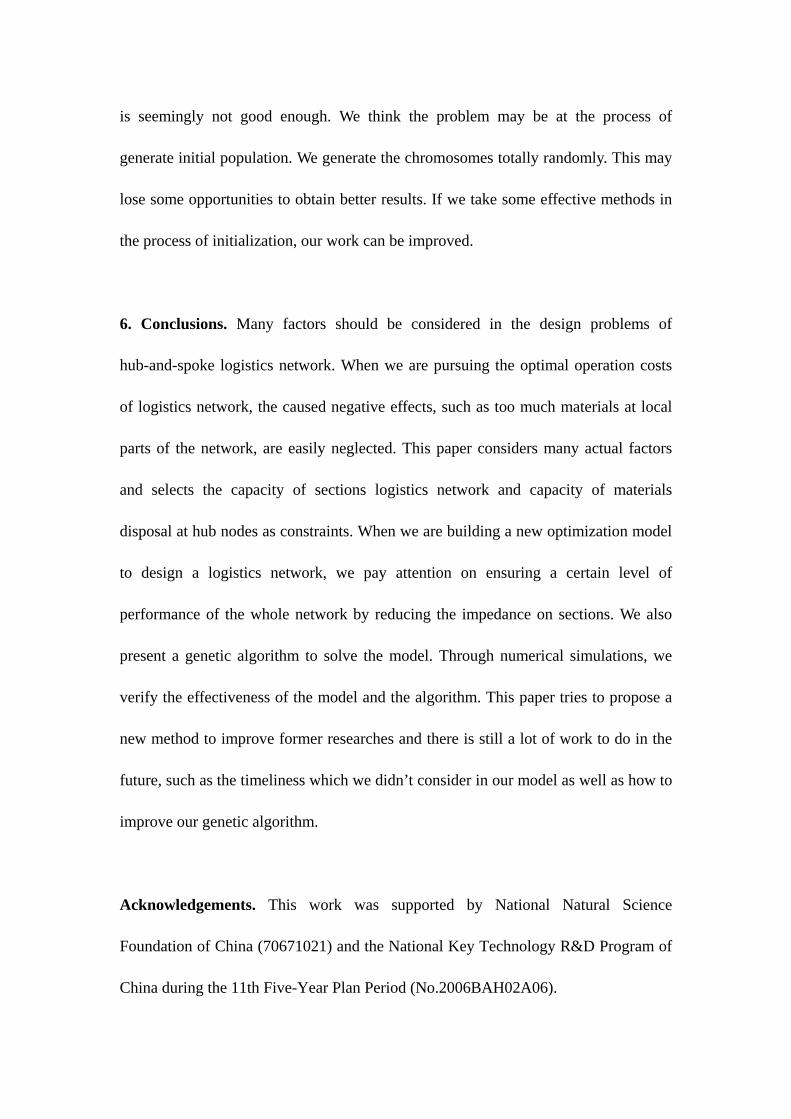
For the number of candidate hub nodes are 6 and we must select 4 hubs in them,

we have 46 15C = different combining forms of hub nodes for H to choose. For each

H, we set a population which contains 100 chromosomes in order to obtain a rather

better result. In addition, we let each population iterate 200 times. Take the first H for

example. Among 200 times iteration, the maximum fitness value of the total

chromosomes in the population which is normalized has the trend shown in Figure 6.

From the curve we can recognize that the algorithm convergences after about 80th

iteration. For at the late stage the most chromosomes are the same and the fitness

value is constituted by normalized cost and time, the fitness value will trend to 2.

6 8 10 12 14 16 18 20 220

5

10

15

20

25

30

FIGURE 5. The initial network

0 20 40 60 80 100 120 140 160 180 2000

0.5

1

1.5

2

2.5

3

FIGURE 6. The trend of fitness value

From Figure 7 and Figure 8, it is obviously that the cost and time both

convergence after about 100th iteration. The result is in accordance with the trend of

fitness value shown in Figure 6. It can illustrate that our genetic algorithm is effective.

By simulation, we obtain some important data for each H. The simulation result is

shown in Table 4. After calculating for each H, we get the best solution with lowest

fitness value respectively. Here we think the cost and time to have equal weight. So

we put them together as the fitness value just after normalization. In practice, if the

any part takes a more important role in improving the performance of network, it may

have bigger weight. In our example, as shown in Table 4, the solution of the second H

has the lowest fitness value. Fortunately, this solution both has the lowest cost and

time, so it is obviously the best choice. Figure 8 shows the best solution.

TABLE 4. Simulation results for 15 Hs

H cost time nor_cost nor_Time fitness value

0 20 40 60 80 100 120 140 160 180 200250

300

350

400

450

500

550

600

FIGURE 8. The trend of time

0 20 40 60 80 100 120 140 160 180 2001.1

.12

.14

.16

.18

1.2

.22

.24

.26x 10

6

FIGURE 7. The trend of cost

1 2 3 4 1115118.8 294.5 0.919 0.849 1.768

1 2 3 5 1077787.4 283.1 0.888 0.816 1.705

1 2 3 6 1106512.2 311.1 0.912 0.897 1.809

1 2 4 5 1213188.2 334.2 1 0.963 1.964

1 2 4 6 1104896.8 317.1 0.911 0.914 1.825

1 2 5 6 1155242.8 317.4 0.952 0.915 1.868

1 3 4 5 1146051.2 299.7 0.945 0.864 1.809

1 3 4 6 1169804.6 335.0 0.964 0.966 1.930

1 3 5 6 1120715.8 303.1 0.924 0.874 1.798

1 4 5 6 1196302.6 346.8 0.986 1 1.986

2 3 4 5 1168306.6 297.3 0.963 0.857 1.820

2 3 4 6 1124887.8 310.3 0.927 0.895 1.822

2 3 5 6 1181590.8 339.9 0.974 0.980 1.954

2 4 5 6 1197646.0 326.9 0.987 0.943 1.930

3 4 5 6 1176842.0 312.0 0.970 0.900 1.870

Though the solution shown in Figure 8 is the best among the solutions we get, it

6 8 10 12 14 16 18 20 220

5

10

15

20

25

30

FIGURE 8. The optimized network

is seemingly not good enough. We think the problem may be at the process of

generate initial population. We generate the chromosomes totally randomly. This may

lose some opportunities to obtain better results. If we take some effective methods in

the process of initialization, our work can be improved.

6. Conclusions. Many factors should be considered in the design problems of

hub-and-spoke logistics network. When we are pursuing the optimal operation costs

of logistics network, the caused negative effects, such as too much materials at local

parts of the network, are easily neglected. This paper considers many actual factors

and selects the capacity of sections logistics network and capacity of materials

disposal at hub nodes as constraints. When we are building a new optimization model

to design a logistics network, we pay attention on ensuring a certain level of

performance of the whole network by reducing the impedance on sections. We also

present a genetic algorithm to solve the model. Through numerical simulations, we

verify the effectiveness of the model and the algorithm. This paper tries to propose a

new method to improve former researches and there is still a lot of work to do in the

future, such as the timeliness which we didn’t consider in our model as well as how to

improve our genetic algorithm.

Acknowledgements. This work was supported by National Natural Science

Foundation of China (70671021) and the National Key Technology R&D Program of

China during the 11th Five-Year Plan Period (No.2006BAH02A06).

REFERENCES

[1] M. K. He, Logistics System Study, Beijing: Higher Education Press, 2004 (in

Chinese).

[2] B. Zou, Exchange Costing Theory—A new angle of study rural industry spatial

pattern, Urban Planning Forum, Vol.31, No.8, pp.8-11, 2001 (in Chinese).

[3] J. G. Klincewica, Hub location in backbone/tributary network design: a review,

Location Science, Vol.6, No.1-4, pp.307-335, 1998.

[4] M. E. O’Kelly, A quadratic integer program for the location of interacting hub

facilities, European Journal of Operational Research, Vol.32, No.3, pp.393-404,

1987.

[5] J. F. Campbell, Integer programming formulationtions of discrete hub location

problems, European Journal of Operational Research, Vol.72, No.2, pp.387-405,

1994.

[6] A. T. Ernst, M. Krishnamoorthy, Exact and heuristic algorithms for the

uncapacitated multiple allocation p-hub median problem, European Journal of

Operational Research, Vol.104, No.1, pp.100-112, 1994.

[7] N. Matsubayashi, M. Umezawa, Y. Masuda, H. Nishino, A cost allocation

problem arising in hub–spoke network systems, European Journal of Operational

Research, Vol.160, No.3, pp.821-838, 2005.

[8] S. Elhedhli, F. X. Hu, Hub-and-spoke network design with congestion, Computer

& Management Sciences, Vol.32, No.6, pp.1615-1632, 2005.

[9] C. C. Lin, S. H. Chen, An integral constrained generalized hub-and-spoke

network design problem, Transportation Research Part E, article in press.

[10] J. G. Klincewica, A dual algorithm for the uncapacitated hub location problem,

Location Science, Vol.4, No.3, pp.173-184, 1996.

[11] S. J. Jeong, C. G. Lee, J. H. Bookbinder, The European freight railway system as

a hub-and-spoke network, Transportation Research Part A: Policy and

Practice, Vol.41, No.6, pp.523-536, 2007.