141

Research Methodology and Sources of Data

In this chapter, we outline the methodology that was used in this research and theoretical

basis behind the approaches. This chapter will describe the methods used to test

hypotheses and research questions. First, in this chapter data collection will be discussed.

Second, Analytical tools will be clarified. Third, questionnaire which is used will be

explained. Fourth, research approach will be investigated. Finally, validity and reliability

will be considered.

4.1 Data Collection

This study attempts to investigate the impact of electronic banking in the Idea. It

explores efficiency, profitability and barriers to the development of electronic banking in

India. A quantitative methodology and econometrics models will be employed to address

the research questions and the hypotheses. This study is based on secondary and primary

data. The required data have been collected from various sources i.e. the primary data

were obtained through questionnaires and were complemented with oral interviews of

experts of IT section and managers of banks involved in the study.

Information and data relating to different banking ratios, banking performance,

volume and number of e-banking transactions and facilities, trend and progress and

different reports and guidelines have been collected from the various annual reports of

RBI, Indian bank’s association, annual reports of selected banks, reports of bank for

international settlement, reports of institute for development and research in banking

technology and IRB bulletins.

4.2 Analytical Tools

For the purpose of analysis of data, a number of financial and statistical

techniques have been used in this study. The tools used for analysis of tables were: Ratio

Analysis, Compound Growth Rate, Annual Average Growth Rate and Growth Rate.

142

In the case of impact of electronic banking on profitability of banking

econometrics models were used. Discovering and understanding the link between

electronic banking and bank performance is an empirical issue. A commonly used

measure of bank performance is the level of bank profits. Bank profitability can be

measured by the return on a bank’s assets (ROA), the ratio of pre-tax profits to equity

(ROE). In this study we use past data for our models.

4.2.1 First Model

In the first model we follow a previous model used by Godarzi and Zabidi (2008)

which ROA is dependent variable. In this model, the number of ATMs is used as an

independent variable to estimate the effect of e-banking on performance of the banking

system in India:

4.2.1.1 Data

This study is based on secondary quantitative data and on panel dataset which

covering 8 top commercial banks of India over the period of 2003-04 to 2010-11. The

banks are State bank of India (SBI), Bank of India (BOI), Central bank of India (CBI),

Punjab national bank (PNB), and Union bank of India (UBI), ICICI Bank, HDFC bank,

and Axis Bank. The data are from banks tables published by RBI and selected banks.

4.2.1.2 Model Specification

The model which we used in this section is based on SCP theory is:

𝑅𝑂𝐴𝑖𝑡 = ∝𝑖+ 𝛽1𝐼𝑀𝐶𝑖𝑡 + 𝛽2𝑆𝐼𝑍𝐸𝑖𝑡 + 𝛽3𝐴𝑇𝑀𝑖𝑡 + 𝛽4 𝑀𝐸𝑀𝐵𝐸𝑅𝑖𝑡 ∗

𝐴𝑇𝑀𝑖𝑡 + 𝜀𝑖𝑡

Where (t) is period of time from 2003 to 2010 and (i) is the number of banks and

other variables of study are:

Dependent variable:

1. ROA: The return on assets (ROA) percentage shows how profitable a

company's assets are in generating revenue.

143

Independent variables:

1. Bank Index of Market Concentration: Proponents of banking sector

concentration argue that economies of scale drive bank mergers and acquisitions

(increasing concentration). Thus, increased concentration goes hand-in-hand with

efficiency improvements. Market concentration is one of the dimensions of the

banking market. This arguably is the most important structural variable in the

equation of profitability. For measurement of concentration in this study we

employed Herfindahl–Hirschman Index. The Herfindahl index (also known

as Herfindahl–Hirschman Index or HHI) is a measure of the size of firms in

relation to the industry and indicator of the amount of competition among them.

𝐼𝑀𝐶𝑖𝑡 = 𝑇𝑜𝑡𝑎𝑙 𝑑𝑒𝑝𝑜𝑠𝑖𝑡 𝑜𝑓 𝑏𝑎𝑛𝑘𝑖 𝑖𝑛 𝑦𝑒𝑎𝑟𝑡𝑇𝑜𝑡𝑎𝑙 𝑑𝑒𝑝𝑜𝑠𝑖𝑡 𝑜𝑓 𝑎𝑙𝑙 𝑏𝑎𝑛𝑘𝑠 𝑖𝑛 𝑦𝑒𝑎𝑟𝑡

2

2. Size (BSIZE): Size of bank is another important structural variable which affects

profitability of banks. It is believed that big banks due to having more

opportunities as compared to small banks are in a better position and their

profitability is higher. This variable in this study is defined as:

𝐵𝑠𝑖𝑧𝑒𝑖𝑡 = 𝑇𝑜𝑡𝑎𝑙 𝑑𝑒𝑝𝑜𝑠𝑖𝑡 𝑜𝑓 𝑏𝑎𝑛𝑘𝑖 𝑖𝑛 𝑦𝑒𝑎𝑟𝑡

3. Number of ATMs: Number of ATMs is another independent variable in this

study. Due to lack of data for other e-banking services we use only numbers of

ATMs as representative of e-banking and period of study will be from 2003-04 to

2010-11.

4. Member to National Financial Switch: Membership to the country’s national

financial switching is a dummy variable in this model and is used to identify

whether membership to financial switching has any impact on profitability of

banks. The Institute of Development and Research in Banking Technology

(IDRBT) in Hyderabad has been providing the ATM switching service to banks in

India through National Financial Switch since 2005.

144

𝑀𝐸𝑀𝐵𝐸𝑅𝑖𝑡 = 0 𝑖𝑓 𝑏𝑎𝑛𝑘 𝑖 𝑛𝑜𝑡 𝑏𝑒 𝑚𝑒𝑚𝑏𝑒𝑟 𝑜𝑓 𝑛𝑒𝑡𝑤𝑜𝑟𝑘 𝑖𝑛 𝑦𝑒𝑎𝑟 𝑡

1 𝑖𝑓 𝑏𝑎𝑛𝑘 𝑖 𝑏𝑒 𝑚𝑒𝑚𝑏𝑒𝑟 𝑜𝑓 𝑛𝑒𝑡𝑤𝑜𝑟𝑘 𝑖𝑛 𝑦𝑒𝑎𝑟 𝑡

4.2.2 Second Model

In order to analyze second model the following empirical models based on previous

works by Berger (1995); Demirguc-Kunt and Huizinga (1999); by Quispe-Agnoli and

Whisler (2006); and Oney et al (2007), is used where we define bank performance, Yit

(measured by the ratio of bank’s pre-tax profits to total assets (ROA) or to its equity

(ROE) for a bank I in year t.

4.2.2.1 Data

In case of second model we will estimate the impact of Internet banking on

performance of the banking industry in India. This model is for eight banks (State bank of

India (SBI), Bank of India (BOI), Central bank of India (CBI), Punjab national bank

(PNB), and Union bank of India (UBI), ICICI Bank, HDFC bank, and Axis Bank ) but

for longer periods of 1997-98 to 2010-11.

4.2.2.2 Model Specification

The model which we used in this section is based on previous work and is:

α0 is a bank fixed effect term that captures time-invariant influences specific to

bank i, MACROt is a matrix of macroeconomic variables in India in year t that include

percentage change in real GDP per capita and the average lending rate charged by banks

in year t. Xit is a matrix of bank-specific control variables: Total deposits in bank i as a

ratio of total assets in year t, total loans of bank i as a ratio of total assets in year t.

20 it

j

ititttitittit INTERNETBANKCRIXMACROY

145

We employ a matrix of dummy variables, INTERNET, that are defined based on

the time of adoption of a transactional website by the bank. Thus, INTERNET is a

dummy variable that equals 1 if the bank introduced a transactional web site in year t.

4.2.3 Estimation Method

In order to estimate equations 1 and 2, there are many econometrics methods. In

this study to estimate the model we used a panel data with eight cross-sections (number

of banks). Panel data analysis is a method of studying a particular subject within multiple

sites, periodically observed over a defined time frame. With repeated observations of

enough cross-sections, panel analysis permits the researcher to study the dynamics of

change with short time series.

To achieve the final model we estimated various linear regression, logarithmic

and semi-logarithmic models via Generalized Least Square (GLS) method on the base of

three models of pooled OLS model, fixed effects and random effects models. All the

independent variables in these models are logarithmic. Generalized least squares (GLS) is

a technique for estimating the unknown parameters in a linear regression model. The

GLS is applied when the variances of the observations are unequal or when there is a

certain degree of correlation between the observations. In these cases Ordinary Least

Squares can be statistically inefficient or even give misleading inferences.

4.2.3 DEA Method

In the case of impact of e-banking on efficiency of banks we use DEA method

(Data Envelopment Analysis). The literature distinguishes two main approaches in

measuring banking efficiency; a parametric and a non-parametric approach in which the

specification of a production cost function is required in both approaches. The parametric

approach engages in the specification and econometric estimation of a statistical or

parametric function, while the non-parametric method offers a linear boundary by

enveloping the experimental data points, known as ”Data Envelopment Analysis” (DEA).

Data Envelopment Analysis (DEA), time to time also called frontier analysis, is a

performance measurement technique which is used to analyze the relative efficiency of

146

productive units. The multiple inputs and multiple outputs are kept the same. It is a non-

parametric analytic technique. This allows us to compare the relative efficiency of the

units as a benchmark by measuring the inefficiencies in input combinations in other units

relative to the benchmark. One of the earliest studies on DEA is the study of Farrell

(1957) who attempted to measure the technical efficiency of production in single input-

output case.

The DEA was originally developed by Charnes, Cooper and Rhodes in 1978.

With their underlying assumption of constant return to scale (CRS) – they attempted to

propose a model that generalizes the single-input to a multiple inputs-outputs setting.

Thus, DMU is an entity that uses input to produce output. DEA was elaborated further by

Banker, Charnes and Cooper (1984). They include the variable of return to scale (VRS)

into the model. The DEA measure, up to that time, was used to evaluate and compare

educational departments, health care, agricultural production, banking, armed forces,

sports, market research, transportation and some other applications.

DEA is a deterministic methodology. For examining the relative efficiency it

relies on the data of selected inputs and outputs of a number of entities called decision–

making units (DMUs). From the set of available data, DEA identifies relative efficiency

of DMUs. These in turn are used as reference points, which define the efficient frontier

and evaluate the inefficiency of other DMUs that lie below that frontier.

DEA is an alternative analytic technique to regression analysis. The regression

analysis approach is characterized as a central tendency approach. That is, it evaluates

DMUs relative to an average. In contrast, DEA is an extreme point method and compares

each DMU with the only best DMU. The main advantage of DEA is that unlike the

regression analysis it does not require an assumption of a functional form relating inputs

to outputs. Instead, it constructs the best production function solely on the basis of

observed data. Hence, statistical tests for significance of the parameters are not necessary

(Chansarn, 2008).

147

4.2.3.1 Return to Scale

Return to scale refers to increasing or decreasing efficiency based on size of the

process of production. For example, a manufacturer can achieve certain economies of

scale by producing thousand Integrated Circuits at the same time rather than one at a

time. It might be only 100 times as hard as producing one at a time. This is an example of

increasing returns to scale (IRS). On the other hand, the manufacturer might find it more

than a trillion times difficult to produce a trillion Integrated Circuits at a time because of

storage problems and limitations on the worldwide Silicon supply. This range of

production illustrates Decreasing Returns to Scale (DRS).

Combining the extreme two ranges would necessitate Variable Returns to Scale

(VRS). Constant Return to Scale (CRS) means that the producers are able to linearly

scale the inputs and outputs without increasing or decreasing efficiency. This is a

significant assumption. The assumption of CRS may be valid over limited ranges but its

use must be justified. But, CRS efficiency scores will never be higher than that of VRS

efficiency scores. In a CRS model, the input-oriented efficiency score is exactly equal to

the inverse of the output-oriented efficiency score. This is not necessarily true for

inefficient DMUs in the case of other return to scale assumptions. The CRS version is

more restrictive than the VRS and yields usually a fewer number of efficient units and

also lower efficient score among all DMUs. In DEA literature the CRS model is typically

referred to as the CCR model after the originators of the seminal publication, by Charnes,

Cooper and Rhodes (1978).

CCR’s model: The model has developed the Farrell’s efficiency measurement

concept from several inputs and one output to several inputs and several outputs. In this

model (Charnes et al., 1978) using a linear combination, different inputs and outputs are

changed into one virtual input and output. The ratio of these virtual combinations of

outputs to inputs is the estimation of efficiency boundary for the measurement of relative

efficiency given that the yield is constant.

BCC’s model: In contrast to the constant yield in the above mentioned model, the

BCC’s model (Banker et al, 1984) assumes a variable output with respect to the scale. In

148

the model, the technical efficiency is decomposed to pure technical efficiency and scaled

efficiency in order to measure the output to scale as well as efficiency itself.

Mathematically, the relative efficiency of a DMU is defined as the ratio of

weighted sum of outputs to the weighted sum of inputs. This can be written as:

𝒉𝒐 = 𝑼𝒓 𝒀𝒓𝒐𝒔

𝒓=𝟏

𝑽𝒊 𝑿𝒊𝒐𝒎

𝒊=𝟏

(1)

Where:

S= number of outputs:

Ur= weight of output r:

Yro= amount of r produced by the DMU:

M=number of inputs:

Vi= weight of input I :and,

Xio= amount of input I used by the DMU:

Equation 1 assumes CRS and controllable inputs. While outputs and inputs can be

measured and entered in this equation without standardization, determining a common set

of weights can be difficult (Avkiran, 1999). DMUs might assess their outputs and inputs

in a different way. This issue is answered in the Charnes, Cooper and Rhodes (known as

CCR) model. Charnes et al. (1978) developed the CCR model that had an input

orientation and assumed CRS. The result of the CCR model indicates a score for overall

technical efficiency (OTE) of each DMU. In other words, this model calculates the

technical efficiency and scale efficiency combined for each DMU. The CCR model

addresses the above problem by allowing a DMU to take up a set of weights that

maximize its relative efficiency ratio without the same ratio for other DMUs exceeding

one. Thus, equation 1 is rewritten in the form of a fractional programming problem:

max ℎ𝑜 = 𝑈𝑟 𝑌𝑟𝑜𝑠

𝑟=1

𝑉𝑖 𝑋𝑖𝑜𝑚

𝑖=1

(2)

Subject to:

149

𝑼𝒓 𝒀𝒓𝒐𝒔

𝒓=𝟏

𝑽𝒊 𝑿𝒊𝒐𝒎

𝒊=𝟏

≤ For each DMU in the sample

Where j=1,……, n (number of DMUs)

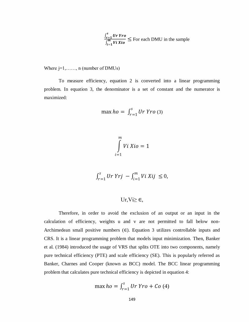
To measure efficiency, equation 2 is converted into a linear programming

problem. In equation 3, the denominator is a set of constant and the numerator is

maximized:

max ℎ𝑜 = 𝑈𝑟 𝑌𝑟𝑜𝑠

𝑟=1 (3)

𝑉𝑖 𝑋𝑖𝑜 = 1

𝑚

𝑖=1

𝑈𝑟 𝑌𝑟𝑗 − 𝑉𝑖 𝑋𝑖𝑗 ≤ 𝑚

𝑖=1

𝑠

𝑟=10,

Ur,Vi≥ ∈,

Therefore, in order to avoid the exclusion of an output or an input in the

calculation of efficiency, weights u and v are not permitted to fall below non-

Archimedean small positive numbers (∈). Equation 3 utilizes controllable inputs and

CRS. It is a linear programming problem that models input minimization. Then, Banker

et al. (1984) introduced the usage of VRS that splits OTE into two components, namely

pure technical efficiency (PTE) and scale efficiency (SE). This is popularly referred as

Banker, Charnes and Cooper (known as BCC) model. The BCC linear programming

problem that calculates pure technical efficiency is depicted in equation 4:

max ℎ𝑜 = 𝑈𝑟 𝑌𝑟𝑜 + 𝐶𝑜𝑠

𝑟=1 (4)

150

𝑉𝑖 𝑋𝑖𝑜 = 1

𝑚

𝑖=1

𝑈𝑟 𝑌𝑟𝑗 − 𝑉𝑖 𝑋𝑟𝑗 − 𝐶𝑜 < 0𝑚

𝑖=1

𝑠

𝑟=1,

Ur,Vi ≥ ∈,

On the whole, the former concerns about the capability of managers to use the

firms’ given resources, while the latter refers to utilizing scale economies by working at a

point where the production frontier approaches the CRS.

To discuss DEA in more detail it is necessary to look at the different concepts of

efficiency. The most common efficiency concept is technical efficiency: the conversion

of physical inputs (such as the services of employees and machines) into outputs relative

to best practice. In other words, given current technology, there is no wastage of inputs

whatsoever in producing the given quantity of output. An organization operating at best

practice is said to be 100% technically efficient. If operating below best practice levels,

then the organization’s technical efficiency is expressed as a percentage of best practice.

Managerial practices and the scale or size of operations affect tech Allocative efficiency

refers to whether inputs, for a given level of output and set of input prices, are chosen to

minimize the cost of production, assuming that the organization being examined is

already fully technically efficient. Allocative efficiency is also expressed as a percentage

score, with a score of 100% indicating that the organization is using its inputs in the

proportions that would minimize costs. An organization that operates at best practice in

engineering terms could still be allocatively inefficient because it is not using inputs in

the proportions which minimize its costs, given relative input prices. Finally, cost

efficiency (total economic efficiency) refers to the combination of technical and

allocative efficiency. An organization will only be cost efficient if it is both technically

and allocatively efficient. Cost efficiency is calculated as the product of the technical and

allocative efficiency scores (expressed as a percentage), so an organization can only

151

achieve a 100% score in cost efficiency if it has achieved 100% in both technical and

allocative efficiency.

4.2.3.2 The Data and Model Specification

This study includes 8 major commercial banks of India, State Bank of India

(SBI), Bank of India (BOI), Central Bank of India (CBI), Punjab National Bank (PNB),

and Union Bank of India (UBI), ICICI Bank, HDFC Bank and Axis Bank. The annual

balance sheet and income statement used were taken from different reports of Reserve

Bank of India. Because of non-availability of data for number of ATMs we analyzed data

from 2003 to 2011.

In the literature in the field, there is no consensus regarding the inputs and outputs

that have to be used in the analysis of the efficiency of the activity of commercial banks

(Berger and Humphrey, 1997). In the studies in the field, five approaches for defining

inputs and outputs in the analysis of the efficiency of a bank were developed, namely: the

intermediation approach; the production approach; the asset approach; the user cost; the

value added approach. The first three approaches are developed according to the

functions that banks do fulfill (Favero and Papi, 1995). The production and the

intermediation approaches are the best known ones and the most used in the

quantification of bank efficiency (Sealy and Lindley, 1997).

In the production-type approach, banks are considered as deposit and loan

producers and it is assumed that banks use inputs such as capital and labor to produce a

number of deposits and loans. According to the intermediation approach, banks are

considered the intermediaries that transfer the financial resources from surplus agents to

the agents with deficit. In this approach it is considered that the bank uses as inputs:

deposits, other funds, equity and work, which they transform into outputs such as: loans

and financial investments. The opportunity for using each method varies depending on

circumstances (Tortosa- Ausina, 2002). The intermediation approach is considered

relevant for the banking sector, where the largest share of activity consists of

transforming the attracted funds into loans or financial investments (Andrie and Cocris,

2010).

152

In our analysis we will use the following set of inputs and outputs to quantify the

efficiency of banks in India:

Outputs: Loans and investments

Inputs: Fixed assets, deposits, number of employees, number of branches and

number of ATMs

This study uses the intermediation approach to define bank inputs and outputs.

Under the intermediation approach, banks are treated as financial intermediaries that

combine deposits, labour and capital to produce loans and investments. Under the

intermediation approach, banks are treated as financial intermediaries that combine

deposits, labour and capital to produce loans and investments. In order to measure

efficiency of banks we employed DEAP Version 2.1 software.

For identification of obstacles and challenges of development of electronic

banking we employed a descriptive and survey research method and also a multistage

sampling method is used as sampling method. In this case we found out and accurately

described the factors that influence implementation and development of electronic

banking.

In the first step of analyzing we used bivariate correlation analysis which

describes the strength, direction and assessing the significance level of the linear

correlation between two variables. These features will help us to test our hypotheses.

There are numbers of different statistics available from SPSS in order to test the

hypotheses, but depending on the level of our measurements all of which are in interval

level we used Pearson Product-Moment Correlation coefficient to test our hypotheses. In

order to evaluate research questions independent sample t-test, one way ANOVA test and

post-hoc are used to evaluate research questions. In the table provided by Pearson

product-moment correlation coefficient there are a number of different aspects of the

output that should be considered. Herein, the first thing to consider is assessing the

significance level to test the hypotheses. If the Sig. value is less than 0.05, then with 95%

confidence there is a correlation between two variables and consequently Null hypotheses

is rejected and the alternative hypothesis is accepted. If the Sig. The value is less than

153

0.01, then with 99% confidence there is a correlation between variables and again Null

hypothesis is rejected. Finally, if the Sig. Value is greater than 0.05, then we conclude

that there is no relationship between variables and accordingly the Null hypothesis is

accepted. In order to determine the direction of the relationships the negative or positive

sign in front of r value will be considered. A negative sign means there is a negative

correlation between two variables (i.e. High scores on one variable is associated with low

scores on the other) and a positive sign means there is a positive correlation between the

two variables (i.e. High scores on one variable is associated with high scores on the

other). For ranking of the challenges we used Friedman test, Friedman test is a

nonparametric test that compares three or more paired groups. The Friedman test ranks

the values in each matched set (each row) from low to high.

4.3 Questionnaire

The questionnaire consists of two sections. The first section gather demographic

information and the second part consists of 36 questions in seven specific sections related

to different challenges in order to explore the respondent’s perceptions about the

challenges and obstacles for the development of e-banking. The 5 point Likert scale is

used for statement of the second section, ranging from extremely agree to extremely

disagree. SPPS 19 software has been used for analysis of questionnaire in this section.

4.4 Research Approach

The methodology of carrying out this research is based on the objectives of this

study. There are two main research approaches to choose from when conducting research

in social science: qualitative or quantitative method. There is one significant difference

between these two approaches. In the quantitative approach, results are based on numbers

and statistics that are presented in figures. But in qualitative approach, the focus lies in

describing an event with the use of words.

In this thesis, different factors that have been emerging from literature review and

theoretical framework are tested in an empirical way in order to see that which factor is a

challenge for development of e-banking and to estimate the impact of e-banking on the

154

performance of banks through different models. Since all the results are presented in

numbers and statistical analyses have been done, quantitative approach is seen as being

appropriate for this study.

4.5 Validity and Reliability

Validity is defined as the instrument’s ability to measure exactly what concepts it

is supposed to measure. If a question can be misunderstood, the information is said to be

of low validity. In order to avoid low validity, we piloted the questionnaire. In addition, a

meeting was arranged in a semi-interview environment and the questions were given to

respondents face to face, so that if they faced any difficulties while filling out the

questionnaire, the ambiguity could be explained and also questions could be modified.

Reliability is about the results of the investigation, which has to be reliable. If

nothing changes in a population between two investigations in the same purpose, it is

reliable. Reliability also refers to the degree to which a measure is free of variable error

also it refers to the accuracy, consistency and stability over time of a measurement

instrument. The collected data have been verified for its reliability using reliability

analysis. Cronbach’s coefficient Alpha has been calculated. The alpha value for 200

questionnaires was found to be 0.809, which indicates the reliability of constructs.

155

References

1. Andrie, A. M. and Cocris, V. (2010): “Comparative Analysis of the Efficiency of

Romanian Banks”, Romanian Journal of Economic Forecasting, Vol.4, pp: 54-75.

2. Bauer Paul, Allen Berger, and David Humphrey. (1992): “Efficiency and

Productivity Growth in US Banking”, in Fried, H. O., Lovell, C.A.K., and

Schmidt, S.S. (Eds.) The Measurement of Productive Efficiency: Technique and

Application, Oxford University Press, New York, pp: 386-413.

3. Berger, A. and Humphrey, D. (1997): “Efficiency of Financial Institutions:

International Survey and Directions for Future Research”, European Journal of

Operational Research, Vol.98, pp: 175-212.

4. Chansarn, S. (2008): “The Relative Efficiency of Commercial Banks in Thailand:

DEA Approach”, International Research Journal of Finance and Economics.

Vol.18, pp: 1450-2887.

5. Sealey, C. and Lindley, J. (1977): “Inputs, Outputs and a Theory of Production

and Cost at Depository Financial Institutions”, Journal of Finance, Vol.32, pp:

1251-1266.

6. Tortosa-Ausina, E. (2002): “Banks Cost Efficiency and Output Specification”,

Journal of Productivity Analysis, Vol.18, pp: 199-222.

7. Yin, R. K. (1994): Case Study Research, Design and Methods, Thousand Oaks:

Sage publications. Inc. California, p: 32.