research for rijksinstituut voor volksgezondheid en …biodiversity indicators for the oecd...
TRANSCRIPT

research forman and environment
RIJKSINSTITUUT VOOR VOLKSGEZONDHEID EN MILIEUNATIONAL INSTITUTE OF PUBLIC HEALTH AND THE ENVIRONMENT
RIVM Report 402001014
Biodiversity indicators for the OECDEnvironmental Outlook and Strategy
A feasibility study
B. ten BrinkFebruary 2000
with a contribution
from the World Conservation Monitoring Centre (WCMC), United Kingdom
Global Dynamics and Sustainable Development Programme
GLOBO REPORT SERIES NO. 25
Commissioned by the Organisation for Economic Co-operation and Development
This investigation has been performed by order and for the account of the OECD, within theframework of project 402001,GEO.
RIVM, P.O. Box 1, 3720 BA Bilthoven, telephone: 31 - 30 - 274 91 11; telefax: 31 - 30 - 274 29 71

page 2 of 52 RIVM report 402001014
National Institute of Public Health and the EnvironmentP.O. Box 13720 BA Bilthoven, The NetherlandsTelephone: 31 30 274 2210(direct)Telefax: 31 30 274 4419 (direct)E-mail: [email protected]
Cover design: Martin Middelburg, Studio RIVM

RIVM report 402001014 Page 3 of 52
Summary
This study addresses the question of feasibility for measuring the trends in nature and its diversityat the OECD level. The answer is ‘yes’, provided certain recommendations are followed.
The study analyzes, in particular, the possibilities of the Natural Capital Index, a frameworkdeveloped and discussed within the Convention on Biodiversity. Here, the key element is to assesschanges in biodiversity as changes in the mathematical product of natural areas (ecosystemquantity) and some measure of the ecosystem quality within the areas. Because data on qualityparameters are not always and everywhere available, the method provides simple protocols to useinformation on various pressure factors in and around the natural area as a fall-back option.
The study provides a review of existing biodiversity indicators and a comparison of majorindicator frameworks. Building on a contribution by the World Conservation Monitoring Strategy,it also provides real-data applications of the Natural Capital approach to the biodiversity in someof the larger ecosystems of the OECD as a preliminary estimation. These include forest, grassland,tundra, inland waters and (semi-) desert.
From this study the Natural Capital Index is concluded to constitute a feasible method forassessing biodiversity in a crude but comprehensive manner. The fall-back option (usinginformation on pressure when information on quality is not available) will make it possible to startusing the framework in the short term. Pressure information will also allow us to make projectionsfor scenario analyses into the future.

page 4 of 52 RIVM report 402001014
Contents
1 INTRODUCTION ...................................................................................................................................5
2 NATURAL CAPITAL INDEX FRAMEWORK ..................................................................................6
2.1 AIMS AND USERS OF THE NCI FRAMEWORK...........................................................................................62.2 THE NCI FRAMEWORK...........................................................................................................................72.3 PRESSURE INDICATORS AS SUBSTITUTE FOR STATE INDICATORS...........................................................142.4 LINKAGE WITH SOCIO-ECONOMIC SCENARIOS ......................................................................................15
3 RESULTS...............................................................................................................................................16
3.1 INTRODUCTION ....................................................................................................................................163.2 ECOSYSTEM QUANTITY ........................................................................................................................16
3.2.1 Example 1: ecosystem quantity assessment................................................................................163.2.2 Example 2: ecosystem quantity assessment in the Global Environment Outlook ......................20
3.3 ECOSYSTEM QUALITY ..........................................................................................................................233.3.1 Example 1: species-abundance of some species groups in the OECD regions..........................233.3.2 Example 2: ecosystem quality assessment in The Netherlands ..................................................263.3.3 Example 3: pressure-based ecosystem quality assessment for Europe ......................................29
4 CONCLUSIONS AND RECOMMENDATIONS...............................................................................33
Literature
Appendix 1: Glossary.......................................................................................................................................37Appendix 2: Ten considerations for choosing quality variables ......................................................................40Appendix 3: List of biodiversity indicators for policy makers..........................................................................41Appendix 4: Review of existing indicators .......................................................................................................42Appendix 5: A comparison of major indicator frameworks ............................................................................48Appendix 6: Defining a baseline for natural and man-made habitats .............................................................50Appendix 7: Specification of natural and man-made ecosystems ....................................................................52
RIVM report 402001014 Page 5 of 52
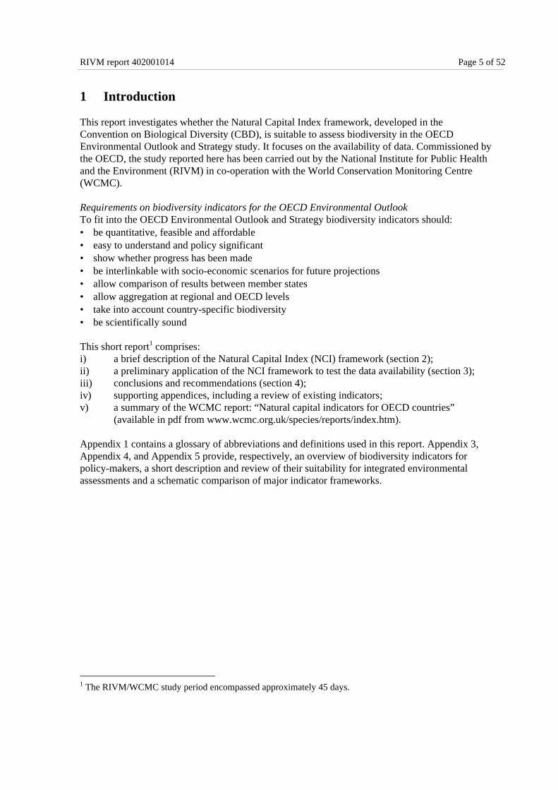
1 Introduction
This report investigates whether the Natural Capital Index framework, developed in theConvention on Biological Diversity (CBD), is suitable to assess biodiversity in the OECDEnvironmental Outlook and Strategy study. It focuses on the availability of data. Commissioned bythe OECD, the study reported here has been carried out by the National Institute for Public Healthand the Environment (RIVM) in co-operation with the World Conservation Monitoring Centre(WCMC).
Requirements on biodiversity indicators for the OECD Environmental OutlookTo fit into the OECD Environmental Outlook and Strategy biodiversity indicators should:• be quantitative, feasible and affordable• easy to understand and policy significant• show whether progress has been made• be interlinkable with socio-economic scenarios for future projections• allow comparison of results between member states• allow aggregation at regional and OECD levels• take into account country-specific biodiversity• be scientifically sound
This short report1 comprises:i) a brief description of the Natural Capital Index (NCI) framework (section 2);ii) a preliminary application of the NCI framework to test the data availability (section 3);iii) conclusions and recommendations (section 4);iv) supporting appendices, including a review of existing indicators;v) a summary of the WCMC report: “Natural capital indicators for OECD countries”
(available in pdf from www.wcmc.org.uk/species/reports/index.htm).
Appendix 1 contains a glossary of abbreviations and definitions used in this report. Appendix 3,Appendix 4, and Appendix 5 provide, respectively, an overview of biodiversity indicators forpolicy-makers, a short description and review of their suitability for integrated environmentalassessments and a schematic comparison of major indicator frameworks.
1 The RIVM/WCMC study period encompassed approximately 45 days.

page 6 of 52 RIVM report 402001014
2 Natural Capital Index framework
2.1 Aims and users of the NCI frameworkOne of the goals of the OECD Environmental outlook and Strategy is to evaluate whether or notprogress has been made on the conservation of biodiversity. This is one of the three major goals ofthe Convention on Biological Diversity (CBD), as shown in Figure 1.
CBD
domesticatedspecies
wildspecies
biodiversityconservation
sustainable use
benefit sharing
biodiversityconservation
sustainable use
benefit sharing
response
state
pressure
• quantity• quality• threatened
Figure 1: Flow chart illustrating in bold the type of indicators examined in this report.They are related to the first of the three objectives of the UN Convention on BiologicalDiversity: i) biodiversity conservation; ii) sustainable use and iii) benefit sharing.. Thisreport deals with both indicators of wild-living biodiversity at the species and ecosystemlevel, and pressure indicators.
The Natural Capital Index (NCI) framework has been developed to assess this -first- Conventionobjective (UNEP, 1997b, 1999). The NCI framework aims at providing a quantitative andmeaningful picture of the state of and trends in biodiversity to support policy makers in a similarway as socio-economic figures support policy makers such as GNP, employment and Price Index.The NCI framework is designed in such a way that it can be applied on all scales -national,regional and global- and for all ecosystems, from forest and marine to agriculture. It deals withwild-living species, not with domesticated species (crops and livestock). The NCI indicators areintended for linkage to socio-economic developments. This enables analysis of socio-economicscenarios on their effect on biodiversity, and makes the NCI framework suitable for integratedenvironmental outlook reports. The state of biodiversity can be given in many detailed figures, butalso in a few or if necessary in one single highly aggregated Natural Capital Index. The OECD

RIVM report 402001014 Page 7 of 52
Environmental Outlook and Strategy will demand for highly aggregated figures. Depending on thebudgets, NCI may be implemented in a fairly simple and affordable way, but a more sophisticatedand expensive way is also possible.
Although the general framework is universal and the results of different OECD countries orregions mutually comparable, the elaboration and implementation is country-specific. Derivativesof the NCI framework have been applied on a global scale to UNEP's Global Environment Outlook(UNEP,1997a) and tested on Europe (Heunks et al., in preparation) and a few countries andecosystems. The development of the framework is an ongoing and open-ended process fed bydiscussions and experiments.
2.2 The NCI framework
Quantity and quality indicatorThe NCI framework provides information on the state and changes in biodiversity due to humaninterventions. It focuses on the changes during industrial times, the period in which loss ofbiodiversity in natural and agricultural ecosystems was accelerating rapidly (UNEP, 1995).
In general the process of biodiversity loss results in a decline in the abundance and distribution ofmany species and the increase in the abundance of a few other species (Figure 2). Speciesextinction is only the last step of a long process of ecosystem degradation.
time
t0 t1 t2Species 1
Species 2
Species 3
Species 4
Figure 2: The essence of biodiversity loss is the decrease in abundance of many speciesand the increase of some other species, due to human interventions. In this illustration theabundance of species 1, 2 and 3 decreases over time while the abundance of species 4rapidly increases.
Note: the decrease in species abundance (numbers of one species) is a far more sensitive indicatorof biodiversity change than the traditional indicator “species richness” (the number of species).Initially the species richness increases from 3 to 4 (in t1) while the average species-abundance of theoriginal species dramatically decreases.

page 8 of 52 RIVM report 402001014
The NCI framework considers biodiversity as a natural resource containing all species with theirspecific abundance, distribution and natural fluctuations. The decrease in abundance of speciesdue to human interference on the one hand and the consequent increase in abundance of otherspecies on the other are considered as a depletion of the “biodiversity resources”, or in other wordsas the depletion of the “natural capital” 2. Globally, habitat loss as a result of converting naturalarea into agricultural and built-up areas is a major causal factor of this loss of natural capital. Thechange in abundance of species in the remaining natural areas due to various pressures such aspollution, exploitation and fragmentation is another major factor (Figure 3).
biodiversity
time
protecteda rea s
ha bita tdestruction
exoticspecies
over exploita tion
pollutiondisturbance
fra gmenta tionclimate cha nge
a ba tementsmeasures
restora tion
susta ina ble use
origina l
Figure 3: The main causes of biodiversity loss and gains. Habitat loss due to landconversion is the major factor. This affects the ecosystem size or “ecosystem quantity”.Other pressures such as over-exploitation and fragmentation change result in loss ofquality in the remaining natural areas. This affects the “ecosystem quality”. Both the lossof ecosystem quantity and ecosystem quality result in the loss of the biodiversity resourceor natural capital.
The loss of biodiversity due both to loss of habitat and to pressures on the remaining habitat arecalled the loss of ecosystem quality and ecosystem quality, respectively. Given these two factorsthe NCI framework has defined the natural capital as the product of the size of the remaining area(ecosystem quantity) and its quality (Figure 5):
NCI =ecosystem quantity × ecosystem quality.
Ecosystem quantity is defined as the size of the ecosystem (% area of country or region).Ecosystem quality is defined as the ratio between the current and a baseline state (% of baseline).(Figure 4).
2 So not only is the extinction of a species a part of the biodiversity loss but also its decline in abundance(numbers of one species). This approach incorporates the spatial aspect of biodiversity which is generallyconsidered very important.

RIVM report 402001014 Page 9 of 52
measures
Present Objective
baseline0% 100%
Figure 4: Ecosystem quality is calculated as a percentage of the baseline state.
The Natural Capital Index (NCI) ranges from 0 to 100%. For example, if 50% of a country stillconsists of natural area and the quality of this area has been decreased to 50%, than the NCI natural
area is 25% (Figure 5). An NCI natural area of 0% means that the entire ecosystem has deterioratedeither because there is no area left, or because the quality is 0% or both. An NCI natural area of 100 %means that the entire country consists of natural area of 100% quality.
quantity
quality
100%
100%0%
50%
50%
25%
NCI100%
Figure 5: Natural capital is defined as the product of the remaining ecosystem size(quantity) and its quality. For example, if the remaining ecosystem size is 50% and itsquality is 50%, then 25% of the natural capital remains. The NCI can be worked out onany spatial scale and for both natural and man-made ecosystems.
The need for a baseline to assess ecosystem qualityA baseline is indispensable in assessing ecosystem quality. Baselines are “starting points” formeasuring change from a certain date or state (Figure 4). For instance, a baseline might be “thenatural state” or “the year the CBD was ratified (1993)”. Although some indicators are used simplyfor comparison over time (for example, the Dow Jones Index and the Price Index), biologicalindicators are far more significant if they are measured against a specific baseline. Setting such a

page 10 of 52 RIVM report 402001014
baseline is a complex and rather arbitrary process. As shown in Box 1 there are many alternativebaselines possible. Each alternative generates a different result and different policy information.For the Natural Capital Index framework various options have been considered by the 1st CBDLiaison Group on Indicators of Biological Diversity including the following (UNEP, 1997b):• at the time that the CBD was ratified• before any human interference• before major interference by industrial society. According to the Liaison Group, measurement against the conditions at the time of the ratificationof the CBD is likely to be an attractive choice. However, using only this baseline raises someimportant questions. How can a change since 1993 be assessed as positive or negative without atheoretical, optimal baseline? (points 2 and 7 in Box 1). Furthermore, only assessing biodiversitywith reference to a baseline set in 1993 (1993 = 100%) would be perceived as a bias towards thedeveloped countries, because these have already achieved a high level of socio-economicdevelopment, partly at the expense of their original biodiversity. Using the state that existed beforeany human intervention would be more appropriate in this respect, but does not appear to befeasible. Since there is no unambiguous natural baseline point in history, and all ecosystems arealso transitory by nature, a baseline must be established at an arbitrary but practical point in time.Because it makes most sense to show the biodiversity change when human influence wasaccelerating rapidly, "a postulated baseline, set in pre-industrial times", further referred to as“natural baseline” or “low-impact baseline”, appears to be most appropriate (Appendix 6). According to the 1st CBD Liaison group, a particular problem relates to the distinction betweenintensively managed, man-made areas on the one hand and self-regenerating or natural3 areas onthe other hand. Comparing, for example, an area of farmland with the original forest, savannah orwetlands system is of little value, because it will simply show that most of the original biodiversityhas disappeared. However, agricultural or other man-made ecosystems might be highly valuedbecause of their cultural-historical values, landscape, and species-richness, even though the lattermay be partly due to introduced (exotic) species.
3 Definitions of natural and man-made ecosystems are given in Appendix 7. The Liaison Group used the word“self-regenerating”areas for “natural” areas. To promote readability this report uses “natural” areas.

RIVM report 402001014 Page 11 of 52
Box 1: Baselines and their role in policy making (Ten Brink, in prep.)
Biodiversity data as such have no meaning. For example: “the currently 1,000 dolphins in the Y-sea” only have significance in relation to baseline values. Baselines make such statisticsmeaningful indicators. The type of baseline determines the policy message. Some examples:
Baseline type
1. Natural state
2. Specific year1993: CBD wasratified
3. Genetically Min.pop. size
4. Red list
5. Speciesrichness
6. None
Baselinevalue4
> 10,000
500
250
750
200species
---
Meaning of current value Vis a vis baseline
Currently 10% of originalpopulation is left. 90% wasdestroyed by anthropogenicfactors, such as pollution,depletion of major fish stocksand drowning in fish nets.
The current population hasbeen doubled
The current population is 4times above the critical level
The current population is 33%above red list criterion
Much of the population canstill be lost without losing aspecies. Even if extirpated itwould not affect the species-richness. An alien seal speciescompensates the loss.
1000 dolphins seems a lot, andthe population appears to begrowing.
Policy signal
The population is still heavilydeteriorated. Let’s work outfurther measures for decisionmaking.
Policy makers did a very goodjob. Fishermen speak about aplague. They propose to limitthe population to 500.Limitation measures?
No need to worry aboutdolphins
Great job done in last years.Dolphins can be removed fromthe red list. “Let’s go back tobusiness”
1000 dolphins is fine but notinteresting. The speciesrichness is only affected whenthe population is zero. Nomeasures are needed, even ifthe dolphins were to disappear.
Fishermen say dolphins arebecoming a plague and mustbe limited. Conservationistsstate that 1000 is not much atall. To restore a healthy marineecosystem it should increase toseveral 1000s. A politicaldiscussion is unavoidable
4 In number of dolphins

page 12 of 52 RIVM report 402001014
The CBD Liaison Group had some important considerations in relation to integratedenvironmental assessment reporting. These are:• the need for aggregation of the state of biodiversity between countries up to regional and global
levels, therefore to have agreed on a scientifically coherent baseline;• the need for comparability of the figures between countries and regions;• the importance of equality between countries, i.e. not setting baselines that favour some regions
over others;• the need for baselines which take into account the specific value of biodiversity in agricultural
landscapes and other man-made habitats.
According to the 1st CBD Liaison Group the pre-industrial baseline is also appropriate to meet theabove needs. The baseline: i) allows for aggregation to a high level, ii) makes figures on countriescomparable, iii) is a fair and common denominator, and iv) is relevant for all habitat types. As forthe latter, natural ecosystems are compared with the low-impact, natural, baseline. Agriculturalecosystems are compared with the traditional agricultural state as baseline, actually beforeindustrialisation of agricultural practices started. This is usually a species-richer state (UNEP,1997b). More information on baselines is given in Appendix 6
considered area
man-made ecosystems
naturalecosystems
distance to cultural baseline distance to natural baseline
qualityassessment
qualityassessment
Figure 6: Man-made ecosystems, mainly agricultural, are assessed by comparing with thetraditional agricultural state as baseline: a “cultural” baseline. Natural ecosystems areassessed by comparing them with a natural or low-impact state as baseline.
Baselines are not targetsIt has to be stressed that baselines serve as a calibration point or benchmark to quantify the extentof change due to human activities in modern times. The baseline is not necessarily the targetedstate. Policy makers choose their targets on ecosystem quantity and ecosystem quality somewhereon the axis between 0 and 100% (Figure 4) depending on their balance of social, economic andecological interests.
Aggregation of data to one single Natural Capital IndexThe natural capital is calculated by the product of the ecosystem quantity and the ecosystemquality. Ecosystem quantity is defined as the percentage of the country’s total area. Ecosystemquality is calculated as a function of many different ecosystem quality variables. To determineecosystem quality it is impossible to measure all species, genes and ecosystem features.

RIVM report 402001014 Page 13 of 52
Operational choices similar to that for socio-economic indicators such as Price Index5 has to bemade. Ecosystem quality is derived from a representative core set of quality variables. These couldbe the abundance of various species, variables on ecosystem structures and species-richness(Figure 7). They are all expressed in terms of percentage of the baseline. These quality variablesare region-specific because each region has his specific species and ecosystems. They could bechosen by each country, but it is also possible to make concerted choices on the level of the OECDregions.
species-abundance variables ecosystem-structure variables
species richnessaverage species abundance average ecosystem structure
b c da s t u v
ecosystem quality indicator unit: % of baseline
selected taxonomic groups
nmlk
ecosystem
aggregation procedure
Figure 7: Ecosystem quality could be determined for example as the average of arepresentative core set of quality variables. These could be variables on speciesabundance, species-richness and ecosystem structure. These are region-specific.
Figure 8 gives an over-all scheme of the NCI framework. Figures can be given in great detail onspecific ecosystems or species as well as highly aggregated or even as one-single index on entirecountries, OECD regions or the OECD as a whole, depending on the purpose.
5 To determine the Price Index or inflation of a country it is not the prices of millions of products that aremonitored in all shops. Instead, a so-called theoretical "shopping bag” is filled with a representative core setof products and subsequently monitored in a subset of shops. The changes in prices are averaged withdifferent weightings because the price increase of bread cannot simply be averaged with the price increase fora car.

page 14 of 52 RIVM report 402001014
(semi)desert
tundragrassland
Natural Capital Index
NCI-man-made
NCI-agriculture
possible aggregation from details
to overall index
NCI-natural
forestmarineNCI
freshwater
quantity(remaining area)
averagequality
quality variables
main habitat types
abcetc.
0 100%
present
20%
baseline
quality per variable
quantity(remaining area)
averagequality
Figure 8: The Natural Capital Index consists of two components: NCI-natural and NCI-man-
made. Each covers various habitat types (third layer). Each habitat type has a quantity (areasize) and a quality (fourth layer) aspect. Ecosystem quality is determined by a core set ofquality variables, which are measured in specific sample areas (fifth layer). The ecosystemquality is calculated by averaging the current/baseline ratios of the core set of qualityvariables.
2.3 Pressure indicators as substitute for state indicatorsIf there are no data on ecosystem quality available a pressure index may be used as substitute toprovide an indication on ecosystem quality. The underlying assumption is that the higher thepressure on biodiversity the lower the probability of high biodiversity (Figure 9). Pressures couldbe climate change, eutrophication, acidification, fragmentation, etc. Often information is availableon current and future pressures based on monitoring and modelling of socio-economic scenarios.When that is the case, each pressure can be graded on a linear scale from pressure 0 (no pressure)to pressure 1000 (very high pressure). Pressure 1000 means high probability of extremely poorbiodiversity compared with the baseline state. For each area the considered pressure values areadded to one single Pressure Index, providing a rough estimation of the probability of highbiodiversity (for more elaboration see UNEP, 1997a; Heunks et al., in prep; RIVM, in prep.).

RIVM report 402001014 Page 15 of 52
10000pressure
Probability ofhigh quality
high
low
Figure 9: A pressure index might be used as substitute for ecosystem quality. This isparticularly interesting if data on the quality of ecosystems are lacking but calculationsare possible on current and future pressures. The assumption is made that the higher thepressure, the lower the probability of high ecosystem quality. The figures 0 and 1000 arederived from values known from literature.
2.4 Linkage with socio-economic scenariosThe NCI framework is designed in such a way that it can be linked to socio-economic scenarios.Ecosystem quantity and quality are both state/impact indicators within the Driving force - Pressure- State - Impact - Response framework (D-P-S-I-R). Ecosystem quantity is directly related to landuse, land cover and physical planning, and can be easily linked to socio-economic scenarios.The use of “abundance of species” as a quality variable for ecosystems is also suitable in thisrespect because species have specific dose−effect relationships to conditions and changes in theenvironment, in contrast to variables at the ecosystem level such as “deciduous forest” or “primaryproduction”. Once the core set of species has been chosen, dose−effect relationships witheutrophication, climate change, fragmentation and exploitation can be investigated and modelled.Subsequently projections can be made on different socio-economic scenarios for each speciesaccording to the cause−effect chain of the D-P-S-I-R model. The change in species abundance ofthe core set of species determines the change in overall ecosystem quality (Figure 24).Other advantages of “species abundance” as quality variable are that species abundance: i) isunambiguously measurable; ii) corresponds to most of the past and current data and monitoringprogrammes; iii) is appealing to policy makers and the public if the species are well chosen; andiv) is sensitive to environmental changes. Although “species-richness” is also a possible qualityvariable, it lacks the above features (Appendix 4). “Ecosystem structure” variables such as the“ratio between dead and living wood” have similar advantages to species abundance.

page 16 of 52 RIVM report 402001014
3 Results
3.1 IntroductionThe WCMC and RIVM have applied the NCI framework on OECD countries. It was investigatedwhether data on ecosystem quality and ecosystem quantity were available or achievable. TheWCMC results are reported separately (WCMC, 1999). The main results of both WCMC andRIVM are given in this section.
3.2 Ecosystem quantity
3.2.1 Example 1: ecosystem quantity assessmentThe aim was to calculate the original and current area of the major natural habitat types: forest,grassland, (semi) desert, tundra and wetland6 for the entire OECD, the OECD regions andindividual countries. Also sought was area information on an intermediate points in time, such as1970, to provide information on recent changes.
The five basic habitat types specified and four OECD continental regions (North America/Mexico,Europe, Japan/Korea, Australia/New Zealand), produce a matrix with 20 cells. However, not allthe habitats of interest occur to a significant extent in all OECD regions, leaving 16 habitat/regioncombinations for which data are required. Void combinations are shaded in Table 1.
Table 1: Habitat and species data coverage (WCMC, 1999).
Forest Grassland desert andsemi-desert
Tundra Wetland
Hab Spp Hab Spp Hab Spp Hab Spp Hab Spp.
N America • • • • • • •
Europe • • • • • •
Japan/Korea •
Australia/NZ • • • •
Note:• indicates data availableempty cells indicate no data locatedshaded cells are void (although some natural grassland exists in Japan/Korea, none is taken into
account in this analysis).Spp: information on the abundance of speciesHab: information on ecosystem size
6 Habitat types according to major habitat types distinguished by the CBD (UNEP, 1997b).

RIVM report 402001014 Page 17 of 52
WCMC used various data sources to calculate the habitat type areas over time. The greatestdifficulty appeared to remain consistent given the different sources and different applieddefinitions of the habitat types, both in time and space. Data on freshwater/wetlands area were notfound, nor were data on the original area of (semi-)desert and tundra, and on an intermediate pointin time (approximately 1970) for all habitat types (see Figure 10, Figure 11, Figure 12 and Table2; WCMC, 1999).
change in forest area
0
1,000,000
2,000,000
3,000,000
4,000,000
5,000,000
6,000,000
7,000,000
8,000,000
9,000,000
1400 1985
period
sqkm
Australia/New ZealandJapan/South KoreaNorth AmericaEurope
Figure 10: Approximate size and change in forest area in OECD regions between 1400and 1985.
Note: 1400 AD represents approximate original area.
change in grassland area and condition
0
500,000
1,000,000
1,500,000
2,000,000
2,500,000
1400 1900 1985
period
sq k
m
Australia/New Zealand
Japan/South Korea
North America
Europe
Figure 11: Approximate size and change in grassland area in OECD regions in 1400,1900 and 1985.
Note: 1400 AD represents original area, 1900 approximate modern area of grassland, and 1985 approximate current extent ofnatural grassland.

page 18 of 52 RIVM report 402001014
change in ecosystem area
0
2000000
4000000
6000000
8000000
10000000
12000000
14000000
16000000
18000000
1400 1985
period
sq k
m forest
grass
Figure 12: Approximate size and change in forest and grassland area in OECD (overall)in 1400 and 1985.
Note: 1400 AD represents approximate original area, and 1985 approximate current extent. Original grassland extent may beunderestimated
The changes in the major habitat types at the regional level according Table 2 are summarised inFigure 13 (WCMC, 1999).

RIVM report 402001014 page 19 of 52
Table 2: Map-based estimates of ecosystem area in the OECD region
Note: nd = no data; past and present areas from different sources.
FORESTAREA
FOREST AREAFOREST
AREAGRASSAREA
GRASSAREA
GRASSQUALITY
GRASSQUALITY
SEMI-DESERT
AREA
DESERTAREA
TUNDRAAREA
past area present areapresent as %
pastpast area present area
present areazero to medium
degradation
present areazero to mediumdegradation as
% total
[defined byhumidity]
[defined byhumidity]
OECD COUNTRIESAustralia 2,314,700 1,433,623 62 531,275 486,228 473,588 97 5,037,185 0 0New Zealand 212,938 42,641 20 15,000 30,000 0
0Japan 375,183 133,285 36 0 0 0 0 0 0South Korea 94,929 15,087 16 0 0 0 0 0 0
0Canada 6,391,481 5,792,705 91 239,985 9,835 7,289 74 225,728 0 1,281,162Mexico 1,115,493 712,262 64 1,103 37,355 10,578 28 863,560 9,896 0United States 587,647 384,376 65 1,765,259 481,192 254,670 53 2,387,169 15,314 610,998
0Austria 79,282 36,633 46 nd 5,575 5,526 99 0 0 0Belgium 29,045 6,874 24 nd 9 3 33 0 0 0Czech Republic 78,602 24,802 32 nd 253 0 0 0 0 0Denmark 43,419 3,704 9 nd 236 236 100 0 0 0Finland 305,464 256,356 84 nd 0 0 0 5,894France 537,846 108,851 20 nd 13,771 10,535 77 274 0 0Germany 349,606 104,070 30 nd 1,882 1,284 68 0 0 0Greece 132,532 45,709 34 nd 11,992 7,055 59 22,703 0 0Hungary 69,849 7,745 11 19,605 1,353 792 59 0 0 0Iceland 36,864 1,229 3 nd 0 0 0 31,413Ireland 60,968 4,567 7 nd 2,005 2,005 100 0 0 0Italy 292,385 68,708 23 nd 11,727 6,454 55 17,874 0 0Luxembourg 2,611 788 30 nd 5 5 100 0 0 0Norway 239,001 113,302 47 nd 0 0 0 89,309Poland 310,751 89,350 29 nd 129 11 9 0 0 0Portugal 88,440 27,054 31 nd 2,799 2,709 97 4,117 0 0Spain 493,915 143,454 29 nd 29,924 20,517 69 148,107 0 0Sweden 410,329 305,873 75 558 13 13 100 0 0 28,807Switzerland 34,796 12,883 37 nd 22 22 100 0 0 0The Netherlands 24,635 2,349 10 nd 244 243 100 0 0 0Turkey 482,361 123,508 26 128,743 0 324,840 0 0United Kingdom 208,142 23,228 11 nd 519 519 100 0 0 0OECD REGIONSAustralia/New Zealand 2,527,638 1,476,264 58 546,275 516,228 473,588 92 5,037,185 0 0Japan/South Korea 470,111 148,372 32 0 0 0 0 0 0North America 8,094,620 6,889,343 85 2,006,347 528,382 272,537 52 3,476,457 25,210 1,892,160Europe 4,310,841 1,511,035 35 148,906 82,458 57,929 70 517,915 0 155,422
OECD (entire) 15,403,210 10,025,014 65 2,701,528 1,127,068 804,054 71 9,031,557 25,210 2,047,582

page 20 of 52 RIVM report 402001014
Figure 13: The changes in the major habitat types at the regional level (WCMC,1999)
Due to the different sources the figures on the different habitat types are inconsistent andmake them difficult to use (WCMC, 1999). Further, the used data sources are not up-datedregularly so they are not suitable to track changes over time. Some data seems to beinaccurate such as the forest-cover figures of the US, which are far too low in comparisonwith FAO data on forest.
3.2.2 Example 2: ecosystem quantity assessment in the Global Environment OutlookRIVM made calculations on the change of natural and man-made areas from 1990 to 2020and 2050 by the IMAGE model (Alcamo et al., 1994a, b and 1998; Klein Goldewijk andBattjes, 1997) for, as an example, UNEP’s Global Environment Outlook (RIVM/UNEP,1997a). Also the original natural land cover and the state in 1890 can be produced (Alcamo etal., 1994a, b, 1998; Klein Goldewijk and Battjes, 1997, derived form Richards, 1990 andFAO, 1990). The area of 5 natural and 2 man-made habitat types is given in Figure 14 forpotential vegetation and the state in the years 1890, 1990, 2010 and 2050. Freshwater area isderived by comparing country area with total land area.
Australia/New Zealand
0
1000000
2000000
3000000
4000000
5000000
6000000
forest past forestpresent
grasslandpast
grasslandpresent
(semi-)desertpast
(semi-)desert
present
tundrapast
tundrapresent
major habitat types
area
(km
2)
Japan/South Korea
0
50000
100000
150000
200000
250000
300000
350000
400000
450000
500000
forest past forestpresent
grasslandpast
grasslandpresent
(semi-)desert past
(semi-)desertpresent
tundra past tundrapresent
major habitat types
area
(km
2)
North America
0
1000000
2000000
3000000
4000000
5000000
6000000
7000000
8000000
9000000
forest past forestpresent
grasslandpast
grasslandpresent
(semi-)desertpast
(semi-)desert
present
tundrapast
tundrapresent
major habitat types
area
(km
2)
Europe
0
500000
1000000
1500000
2000000
2500000
3000000
3500000
4000000
4500000
5000000
forest past forestpresent
grasslandpast
grasslandpresent
(semi-)desertpast
(semi-)desertpresent
tundrapast
tundrapresent
major habitat types
area
(km
2)

RIVM report 402001014 page 21 of 52
0%
10%
20%
30%
40%
50%
60%
70%
80%
90%
100%
1 2 3 4 5
Land cover/use changes in OECD North America1= potential vegetation, 2 = 1890, 3 = 1990 and 4 = 2020, 5 = 2050
ameri
0%
10%
20%
30%
40%
50%
60%
70%
80%
90%
100%
1 2 3 4 5
Land cover/use changes in OECD Asia1= potential vegetation, 2 = 1890, 3 = 1990 and 4 = 2020, 5 = 2050
0%
10%
20%
30%
40%
50%
60%
70%
80%
90%
100%
1 2 3 4 5
Land cover/use changes in OECD Oceania1= potential vegetation, 2 = 1890, 3 = 1990 and 4 = 2020, 5 = 2050
0%
10%
20%
30%
40%
50%
60%
70%
80%
90%
100%
1 2 3 4 5
Land cover/use changes in OECD Europe1= potential vegetation, 2 = 1890, 3 = 1990 and 4 = 2020, 5 = 2050
0%
10%
20%
30%
40%
50%
60%
70%
80%
90%
100%
1 2 3 4 5
Land cover/use changes in OECD countries1 = potential vegetation, 2 = 1890, 3 = 1990, 4 = 2020, 5 = 2050
Desert
Grasslands, steppe
Forest
Tundra
Ice
Domesticated(marginal)
Domesticated(intensive)
Figure 14: Land cover of two man-made and five natural habitat types as potentialvegetation and in the years 1890, 1990, 2020 and 2050 (Alcamo, 1994) in the OECD regionsand total OECD.
Note: North America: Canada, USA, Mexico; Asia: Japan, South Korea. Oceania: Australia, NewZealand; Europe: Western Europe, incl. Hongary, Polen, Czech republic, Turkey

page 22 of 52 RIVM report 402001014
The spatial scale of the IMAGE model is approximately 50 by 50 km around the equator.Although the figures are course, they have the advantage of being consistent in time andspace. Calculations are possible for socio-economic scenarios. The information is geo-referenced so maps can be drawn. For small countries it is inaccurate. At the level of regionsit provides a first estimate of the changes over time.
Another data source is the Pan European Land Cover Monitoring project which determinesthe current European land cover on a 1 km2 basis (Figure 15). Although this information is gathered on a regular basis from satellites (NOAA)the results appears to be still too in-accurate to track changes in time within a period less than20 years (Heunks et al., in prep.). It does not provide information on the past. Nevertheless,new remote sensing techniques with various satellite images and the use of lidar and radar(multi scale and multi spectral approach) provide most promising possibilities on a moreaccurate global monitoring of habitat types within 5 to 10 years (Pelcom workshop, 1999).
Figure 15: Map of the natural areas in pan-Europe in 1990 on the basis of adaptedNOAA satellite data (Heunks et al., in prep.). The colours provide additionalinformation on the pressure to Europe’s natural areas (green low, violet high) basedon ozone, acidification, eutrofication, temperature change, isolation, population andGDP (see further section 3.3.3).

5,90�UHSRUW���������� SDJH����RI���
���� (FRV\VWHP�TXDOLW\:KLFK�LQIRUPDWLRQ�LV�GLUHFWO\�DYDLODEOH�RQ�WKH�TXDOLW\�RI�WKH�PDMRU�QDWXUDO�KDELWDW�W\SHV"�)RU
HDFK�RI�WKH�2(&'�UHJLRQV��:&0&�VHOHFWHG�VSHFLHV�RQ�ZKLFK�GDWD�RQ�WKH�FKDQJH�LQ�WKHLU
SRSXODWLRQV�RU�GLVWULEXWLRQ�LQ�WKH�ODVW����\HDUV�ZHUH�DYDLODEOH��%DVHOLQH�LQIRUPDWLRQ�ZDV�DOVR
VRXJKW��7KH�EDVHOLQH�VWDWH�LV�WKH�H[SHFWHG�RU�RULJLQDO�VWDWXV�RI�WKH�SRSXODWLRQV�LQ�WKHVH�DUHDV�LI
QRW�RU�KDUGO\�DIIHFWHG�E\�KXPDQV��5,90�KDV�DGGHG��DV�H[DPSOH���VSHFLHV�DEXQGDQFH
LQIRUPDWLRQ�DYDLODEOH�RQ�D�QDWLRQDO�EDVLV��7KH�1HWKHUODQGV��DQG�IRU�(XURSH�LQIRUPDWLRQ
DYDLODEOH�RQ�SUHVVXUHV��VXEVWLWXWLQJ�IRU�VWDWH�LQGLFDWRUV�
������ ([DPSOH����VSHFLHV�DEXQGDQFH�RI�VRPH�VSHFLHV�JURXSV�LQ�WKH�2(&'�UHJLRQV
7KH�UHVXOWV�DUH�SUHVHQWHG�LQ�)LJXUH������)LJXUH�����)LJXUH�����)LJXUH�����)LJXUH����DQG�)LJXUH
����:&0&��������
�
���
���
���
���
�
���
���
���
���� ���� ���� ���� ���� ����
)LJXUH�����(XURSH��IRUHVW�VSHFLHV
1RWH��$YHUDJH�FKDQJH�LQ�SRSXODWLRQ�VL]H�FRPSDUHG�ZLWK�������EDVHG�RQ�GDWD�IRU����ELUG�VSHFLHV�
�
���
���
���
���
�
���
���
���� ���� ���� ���� ���� ���� ����
)LJXUH������1RUWK�$PHULFD��IRUHVW�VSHFLHV
1RWH��$YHUDJH�FKDQJH�LQ�SRSXODWLRQ�VL]H�FRPSDUHG�ZLWK�������EDVHG�RQ�GDWD�IRU�����ELUG�VSHFLHV�

SDJH����RI��� 5,90�UHSRUW����������
�
���
���
���
���
�
���
���� ���� ���� ���� ����
)LJXUH�����(XURSH��JUDVVODQG�VSHFLHV
1RWH��$YHUDJH�FKDQJH�LQ�SRSXODWLRQ�VL]H�FRPSDUHG�ZLWK��������EDVHG�RQ�GDWD�IRU���ELUG�VSHFLHV�
�
� � �
� � �
� � �
� � �
�
� � �
� � � � � � � � � � � � � � � � � � � � � � � � � � � �
)LJXUH�����1RUWK�$PHULFD��JUDVVODQG�VSHFLHV
1RWH��$YHUDJH�FKDQJH�LQ�SRSXODWLRQ�VL]H�FRPSDUHG�ZLWK�������EDVHG�RQ�GDWD�IRU����ELUG�VSHFLHV�
�
���
���
���
���
�
���
���
���
���
�
���� ���� ���� ���� ����
)LJXUH�����$XVWUDOLD�1HZ�=HDODQG��VHPL�GHVHUW�VSHFLHV
1RWH��$YHUDJH�FKDQJH�LQ�SRSXODWLRQ�VL]H�FRPSDUHG�ZLWK�������EDVHG�RQ�GDWD�IRU���PDPPDO�VSHFLHV�

5,90�UHSRUW���������� SDJH����RI���
�
���
���
���
���
�
���
���
���
���
�
���
���
���
���
�
���
���
���
���
�
���
���� ���� ���� ���� ���� ���� ����
)LJXUH�����1RUWK�$PHULFD��WXQGUD�VSHFLHV
1RWH��$YHUDJH�FKDQJH�LQ�SRSXODWLRQ�VL]H�FRPSDUHG�ZLWK�������EDVHG�RQ�GDWD�IRU���ELUGV�DQG�WZR
PDPPDOV�
:LWKLQ�WKH�OLPLWV�RI�WKH�:&0&�VWXG\�LW�GRHV�QRW�DSSHDU�WR�EH�IHDVLEOH�WR�FROOHFW�EDVHOLQH�GDWD�
%DVHOLQH�GDWD�DUH�YHU\�LPSRUWDQW�LQ�WKLV�UHVSHFW�LI�DQ�DSSURSULDWH�DVVHVVPHQW�RI�WKH�TXDOLW\�RI
WKH�UHPDLQLQJ�QDWXUDO�DUHDV�LV�WR�EH�PDGH��%R[�����$OWKRXJK�WKH�$PHULFDQ�IRUHVW�VSHFLHV��IRU
H[DPSOH��DSSHDUV�WR�EH�VWDEOH�LQ�WKHLU�DEXQGDQFH�LQ�UHFHQW�WLPHV��LW�PLJKW�EH�ZHOO�SRVVLEOH�WKDW
WKH�TXDOLW\�DV�VXFK�LV�VWLOO�ORZ�WR�GDWH��)LJXUH�����
EDVHOLQH ���� ����
3RSXODWLRQ�VL]H
WLPH
$
%
)LJXUH�����%DVHOLQH�LQIRUPDWLRQ�LV�LQGLVSHQVDEOH�IRU�DVVHVVLQJ�WKH�FXUUHQW�TXDOLW\�RI
DQ�HFRV\VWHP��$�EDVHOLQH�DFFRUGLQJ�WR�RSWLRQ�$�PHDQV�WKDW�WKH�TXDOLW\�RI�WKH�ODVW���
\HDUV�LV�VWDEOH�EXW�ORZ��ZKLOH�D�EDVHOLQH�DFFRUGLQJ�WR�RSWLRQ�%�PHDQV�WKDW�WKH�TXDOLW\
LV�VWDEOH�DQG�KLJK�
)XUWKHU��LQIRUPDWLRQ�RQ�PRUH�VSHFLHV�JURXSV�WKDQ�ZKLFK�DUH�JLYHQ�KHUH�LV�QHFHVVDU\�WR�SURYLGH
D�UHDVRQDEOH�UHSUHVHQWDWLYH�SLFWXUH�RI�WKH�TXDOLW\�RI�WKH�PDMRU�KDELWDW�W\SHV��:&0&�DVVHVVHV�LW
DV�EHLQJ�TXLWH�SRVVLEOH�WR�JHW�EDVHOLQH�LQIRUPDWLRQ�DQG�LQIRUPDWLRQ�RQ�PRUH�JURXSV�ZLWKLQ�WKH
FRXQWULHV�WKHP�VHOYHV��VHH�H[DPSOH�QH[W�VHFWLRQ��

page 26 of 52 RIVM report 402001014
3.3.2 Example 2: ecosystem quality assessment in The NetherlandsRIVM has worked out a case study on the ecosystem quantity and quality of the Dutchnatural and agricultural ecosystems (Ten Brink et al.; 1998; RIVM, 1999). The populationnumbers of about 350 plant species, 30 butterfly species, 90 bird species and 60 marine andriver species were determined for the baseline state (1900 to 1950) and the current state(1990). Appendix 2 lists ten considerations for choosing these species. Figure 23 providesinformation -as an example- on the marine ecosystem. It shows the significant shifts in theabundance of species in 60-90 years as a result of various human pressures such aseutrophication (algae, benthic species, birds), fisheries (fish stock depletion, cockle beds,mussel beds), contamination (seal, dolphin), disturbance (seal, dolphin, tern), turbidity (seagrass) and damming/habitat loss (sturgeon, sea grass, salt marshes). Overall, a shift can beseen from long-lived to short-lived species.
Situation 1988
Present
Reference (1930)
(sea-amoeba)
Phaeocystis
Sea Lettuce
Channel Wrack
Kelp
Sea Grasses
Salt Marshes
Cockle beds
Wild Mussel beds
Baltic Tellin
Sand Gaper
Shrimp
Common Dog WhelkSea Potato
Plumose AnemoneLobster
HerringCod
Rays
Sturgeon
Plaice
Guillemot
Brent Goose
Eider
Oystercatcher
Avocet
Dunlin
Common SealHarbour Porpoise
Bottlenose
Sandwich TernTotal Algae
Dolphin
Fulmar Petrel
Figure 23: A core set of 32 species has been selected to describe and assess the stateof the North Sea. The abundance of each species is calculated for the baseline state(period 1900-1930) and the current state (1988) and presented in a radar-diagram.The radius from the centre to the circle represents the baseline numbers (100%), thecurrent numbers are superimposed on this circle and connected with a line, forminga star-like figure (Ten Brink et al. 1991). The average ecosystem quality is in thiscase 50%.
RIVM report 402001014 page 27 of 52
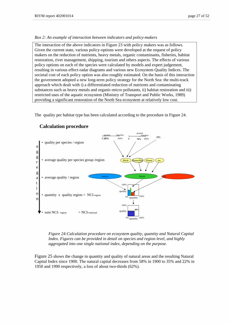
Box 2: An example of interaction between indicators and policy-makers
The interaction of the above indicators in Figure 23 with policy makers was as follows.Given the current state, various policy-options were developed at the request of policymakers on the reduction of nutrients, heavy metals, organic contaminants, fisheries, habitatrestoration, river management, shipping, tourism and others aspects. The effects of variouspolicy options on each of the species were calculated by models and expert judgement,resulting in various effect-radar diagrams and various new Ecosystem Quality Indices. Thesocietal cost of each policy option was also roughly estimated. On the basis of this interactionthe government adopted a new long-term policy strategy for the North Sea: the multi-trackapproach which dealt with i) a differentiated reduction of nutrients and contaminatingsubstances such as heavy metals and organic-micro pollutants, ii) habitat restoration and iii)restricted uses of the aquatic ecosystem (Ministry of Transport and Public Works, 1989)providing a significant restoration of the North Sea ecosystem at relatively low cost.
The quality per habitat type has been calculated according to the procedure in Figure 24.
Calculation procedure
• quality per species / region
• average quality per species group /region
• average quality / region
• quantity x quality region = NCI-region
• sum NCI- region = NCI-national
aggregation
0 100%
present
20%baseline
forest
0 100%
presentbaseline
70%
Birds Butterflies Plants etc.
etc.
etc marine
0%
100%
100%
quality
quantity
100%
100%
0%
40%quality
quantity
Figure 24:Calculation procedure on ecosystem quality, quantity and Natural CapitalIndex. Figures can be provided in detail on species and region level, and highlyaggregated into one single national index, depending on the purpose.
Figure 25 shows the change in quantity and quality of natural areas and the resulting NaturalCapital Index since 1900. The natural capital decreases from 58% in 1900 to 35% and 22% in1950 and 1990 respectively, a loss of about two-thirds (62%).

page 28 of 52 RIVM report 402001014
100%
50%
0% 50% 100%
Quantity
Quality
1900
1997
100%
NCI-natural
1950
1990
58%
35%
22%
2020?
Figure 25: Quantity and quality of natural area (aquatic and terrestrial) in 1900,1950 and 1990. The quantity (horizontal) and quality (vertical) of the Dutch naturalecosystems dramatically declined since 1900.
Figure 26 shows the change in quantity and quality of the Dutch agro-ecosystems and aresulting agro-Natural Capital Index since 1900.
50% 100%0%
Quantity
100%
NCI-man-made
1900
1950
1990
38%
48%
20%
Quality
50%
100%
Figure 26: Quantity and quality of man-made area (mainly agricultural area, a fewurban areas) in 1900, 1950 and 1990. The man-made area expended from 41% to52% and 55% in respectively 1900, 1950 and 1990 (horizontal). The qualitydramatically declined from 90% in 1900/1950 to 37% in 1990 (vertical). A slightquality loss is due to –low quality- urban area.
The agricultural area expanded, mostly until 1950, but its quality declined significantly since1950. Quantity and quality combined, there was an increase on the agro-Natural CapitalIndex from 38% to 48% in the first half of the century, and, subsequently, a decrease to 20%in the second half. This first estimation shows that about 60% of the agro-biodiversity waslost since 1950.

RIVM report 402001014 page 29 of 52
3.3.3 Example 3: pressure-based ecosystem quality assessment for EuropeIf data on the state of ecosystems are lacking, pressures might be used as substitute. At theGlobal and European levels a pressure based approach was worked out for UNEP’s GlobalEnvironment Outlook (UNEP, 1997a) and has been further elaborated and applied for thePriority Study on European Environmental Problems (RIVM, in prep). For the formerapplication is referred to the UNEP document. The latter example is summarised here:
For the study on Europe the remaining natural area and the sum of 7 pressures have beencalculated on a grid cell basis of 1 km2 for 1990 and 2020 according to the Baseline scenario.These seven pressures are: climate change; human population density; consumption andproduction intensity per km2; fragmentation; eutrophication; acidification and ozoneconcentrations. This selection was pragmatic because: i) these pressures could be calculatedfor 1990 and projected for 2010 on a regional basis, ii) these pressures represent differentsupplementary types of pressures, and iii) from the literature knowledge was available ondose-effect relationships and critical levels. Each pressure is preliminarily graded on a linearscale from pressure 0 (no pressure) to pressure 1000 (very high pressure (Figure 9, Table 3).Pressure 1000 means high chances of extremely poor biodiversity compared with the baselinestate. For each grid cell the seven pressure values were added (maximum 7000) to one singlePressure Index. A Pressure Index of >2500 is considered as extremely high and,consequently, has low chances on attaining high ecosystem quality.
Table 3: Pressures to biodiversity and scaling values.
Pressures High chance on high ecosystemqualityPressure = 0
Low chance on high ecosystemqualityPressure = 1000
1. Rate of climate (temperature) change < 0.2°C change in 20 years > 2.0°C change in 20 years2. Human population density < 10 persons/km2 > 150 persons/km2
3. Consumption and production (GDP) US$ 0 per km2 > US$ 6,000,000 per km2
4. Isolation/fragmentation % natural area within 10 km > 64% % natural area within 10 km < 1%5. Acidification Deposition < critical load Deposition > 5 x critical load Cl5%
6. Eutrofication Deposition < critical load Deposition > 5 x critical load Cl5%
7. Exposure to high ozone conc. AOT40 < critical level AOT40 > 5 x critical level
Table 4 and Table 5 present the individual and total pressures per country, as well as apressure-based NCI for 1990 and 2010 according to the Baseline Scenario.
The extent and distribution of Europe’s natural areas and the pressure on them in 1990 and2010 are presented inFigure 15 and Figure 27, respectively.
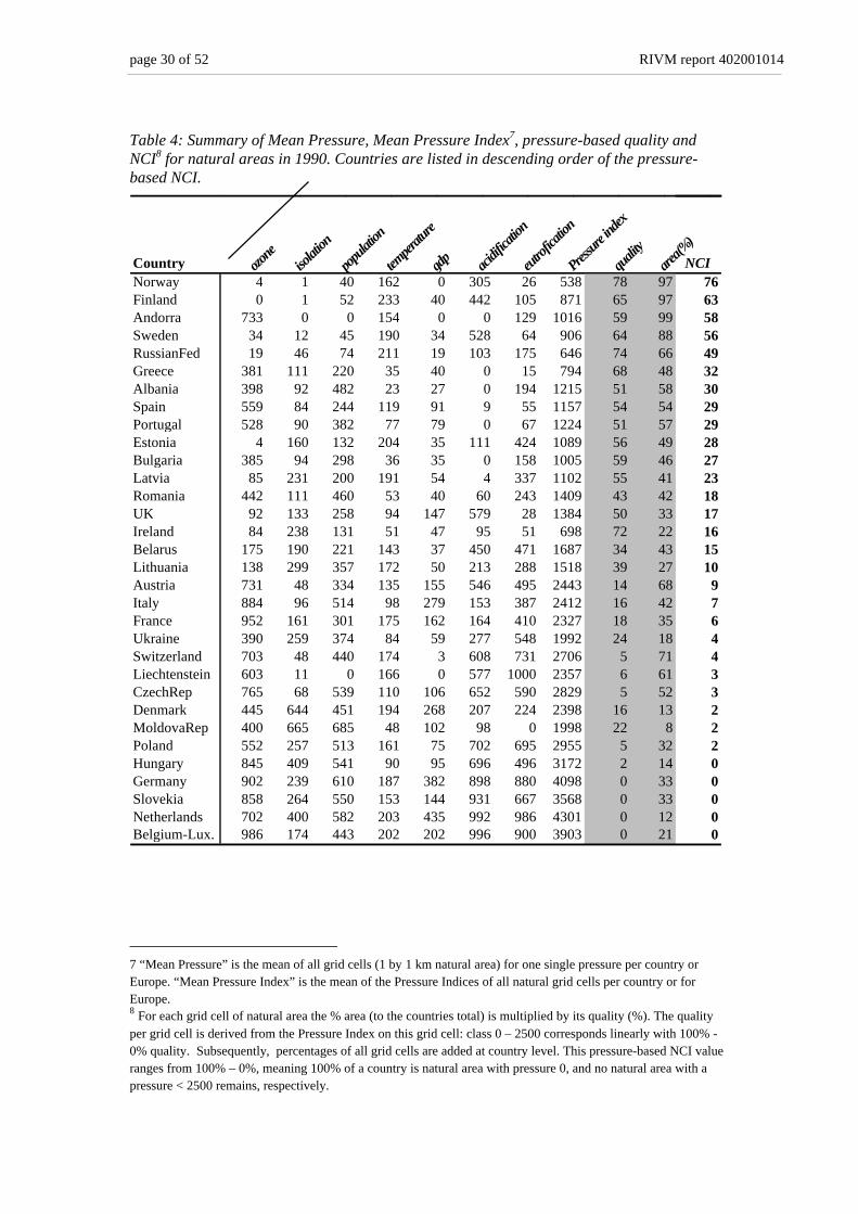
page 30 of 52 RIVM report 402001014
Table 4: Summary of Mean Pressure, Mean Pressure Index7, pressure-based quality andNCI8 for natural areas in 1990. Countries are listed in descending order of the pressure-based NCI.
Country ozone
isolat
ion
popu
lation
temper
ature
gdp acidif
icatio
n
eutro
ficati
on
Pressur
e index
quali
tyare
a(%)
NCINorway 4 1 40 162 0 305 26 538 78 97 76Finland 0 1 52 233 40 442 105 871 65 97 63Andorra 733 0 0 154 0 0 129 1016 59 99 58Sweden 34 12 45 190 34 528 64 906 64 88 56RussianFed 19 46 74 211 19 103 175 646 74 66 49Greece 381 111 220 35 40 0 15 794 68 48 32Albania 398 92 482 23 27 0 194 1215 51 58 30Spain 559 84 244 119 91 9 55 1157 54 54 29Portugal 528 90 382 77 79 0 67 1224 51 57 29Estonia 4 160 132 204 35 111 424 1089 56 49 28Bulgaria 385 94 298 36 35 0 158 1005 59 46 27Latvia 85 231 200 191 54 4 337 1102 55 41 23Romania 442 111 460 53 40 60 243 1409 43 42 18UK 92 133 258 94 147 579 28 1384 50 33 17Ireland 84 238 131 51 47 95 51 698 72 22 16Belarus 175 190 221 143 37 450 471 1687 34 43 15Lithuania 138 299 357 172 50 213 288 1518 39 27 10Austria 731 48 334 135 155 546 495 2443 14 68 9Italy 884 96 514 98 279 153 387 2412 16 42 7France 952 161 301 175 162 164 410 2327 18 35 6Ukraine 390 259 374 84 59 277 548 1992 24 18 4Switzerland 703 48 440 174 3 608 731 2706 5 71 4Liechtenstein 603 11 0 166 0 577 1000 2357 6 61 3CzechRep 765 68 539 110 106 652 590 2829 5 52 3Denmark 445 644 451 194 268 207 224 2398 16 13 2MoldovaRep 400 665 685 48 102 98 0 1998 22 8 2Poland 552 257 513 161 75 702 695 2955 5 32 2Hungary 845 409 541 90 95 696 496 3172 2 14 0Germany 902 239 610 187 382 898 880 4098 0 33 0Slovekia 858 264 550 153 144 931 667 3568 0 33 0Netherlands 702 400 582 203 435 992 986 4301 0 12 0Belgium-Lux. 986 174 443 202 202 996 900 3903 0 21 0
7 “Mean Pressure” is the mean of all grid cells (1 by 1 km natural area) for one single pressure per country orEurope. “Mean Pressure Index” is the mean of the Pressure Indices of all natural grid cells per country or forEurope.8 For each grid cell of natural area the % area (to the countries total) is multiplied by its quality (%). The qualityper grid cell is derived from the Pressure Index on this grid cell: class 0 – 2500 corresponds linearly with 100% -0% quality. Subsequently, percentages of all grid cells are added at country level. This pressure-based NCI valueranges from 100% – 0%, meaning 100% of a country is natural area with pressure 0, and no natural area with apressure < 2500 remains, respectively.

RIVM report 402001014 page 31 of 52
Table 5: Summary of Mean Pressure, Mean Pressure Index7, pressure-based quality andNCI8 for natural areas for 2010 in the Baseline Scenario. Countries are listed in descendingorder of the pressure-based NCI.
Country ozone
isolat
ion
popu
lation
temper
ature
gdp acidif
icatio
n
eutro
ficati
on
Pressur
e index
quali
ty(%)
area(%
)
NCIFinland 0 1 57 378 56 11 29 531 78 98 77Norway 1 1 43 278 58 279 3 664 73 97 71Andorra 414 0 0 270 0 0 63 748 70 99 69Sweden 8 12 49 317 50 141 18 593 76 91 69RussianFed 3 46 73 347 18 8 60 517 79 87 69Greece 271 111 226 104 58 0 9 714 71 65 46Estonia 0 160 124 339 40 2 217 868 65 55 35Albania 275 92 545 85 36 0 151 1166 53 61 33Bulgaria 306 94 277 102 44 0 95 909 63 49 31Spain 366 84 247 225 137 0 29 1069 57 52 30Latvia 9 231 202 320 50 0 165 932 62 47 29Portugal 386 90 383 165 135 0 49 1195 52 54 28Belarus 35 190 219 250 42 82 311 1089 56 49 28Austria 421 48 408 240 273 58 307 1749 34 71 24Romania 312 111 447 124 51 24 182 1240 50 46 23UK 53 133 263 181 198 273 3 1131 60 36 21Liechtenstein 336 11 0 288 0 48 1000 1683 33 61 20Lithuania 20 299 362 295 45 20 162 1147 54 36 19Ireland 30 238 143 121 111 0 28 639 74 21 16Ukraine 211 259 368 167 48 54 413 1421 43 31 13France 622 161 319 299 220 36 245 1879 30 40 12CzechRep 479 68 574 203 141 341 354 2145 19 56 11Italy 647 96 514 192 374 55 290 2131 23 39 9Switzerland 416 48 472 295 474 282 588 2577 12 71 9Poland 309 257 532 275 135 71 447 2006 24 34 8MoldovaRep 211 665 686 115 60 33 0 1650 34 21 7Denmark 201 644 447 324 362 101 90 2079 24 20 5Slovekia 498 264 560 265 199 187 361 2310 13 35 5Netherlands 485 400 586 339 527 405 617 3327 20 16 3Germany 542 239 617 313 429 412 444 2974 7 36 2Belgium-Lux. 849 174 459 334 282 428 641 3141 6 23 1Hungary 541 409 518 177 133 534 361 2646 7 17 1

page 32 of 52 RIVM report 402001014
Figure 27: Pressure map of the natural areas in pan-Europe for 2010 in the BaselineScenario on the basis of adapted NOAA satellite data (Heunks et al., in prep.). Thecoloured areas show the extent and distribution of Europe’s remaining naturalareas. The colour provide information on the pressures ranging from low (green) toextremely high (violet) based on ozone, acidification, eutrophication, temperaturechange, isolation, population and GDP.
The above case studies illustrate what could be possible when pressures are used as substituteinformation for ecosystem quality. It should be clearly emphasised that there are limitationsto the implementation presented here. There are other, particularly local, factors whichshould be taken into account, such as forestry, water use, hunting, fire, infrastructure andextensive cattle grazing. Dose-effect relationships could be improved and better underpinnedand differentiated for regions and habitat types. There is uncertainty in the modelling andprojections for the future. In the longer term, the use of state indicators in preference topressure indicators will provide a more direct picture of biodiversity it self. Nevertheless thispressure-based biodiversity assessment tool could provide useful policy information in theshort term to assess efficacy of policy options.

RIVM report 402001014 page 33 of 52
4 Conclusions and recommendations
The goal of this study is to investigate whether the NCI framework could be a feasible,significant and universal assessment methodology for OECD’s Environmental Outlook forthe near future. Although preliminary estimations of baseline figures for species abundance,intermediate time points and wetlands were not feasible within the limitations of this study, itcan be concluded that the NCI framework appears a realistic opportunity because (or if):
1. The Natural Capital Index framework meets OECD’s requirementsThe Natural Capital Index framework appears to be a suitable indicator framework forthe state of the natural capital at the country, OECD-region and entire OECD levels,meeting the requirements for the OECD Environmental Outlook in section 1.
2. Countries are able to determine the change in major-habitat size (bottom up)The size of the major habitat types can be best determined by the member states withnational land-cover statistics. Generally they are periodically up-dated. Within 5-10 yearsremote sensing data could be a possible alternative –global- data source to track changes,provided that the accuracy of these data is highly improved.
3. The distinction of just a few major habitat types advances the feasibilityBecause ecosystems tend to grade into one another, there are fundamental logicaldifficulties in demarcating ecosystem boundaries and in classifying habitat types. Tominimise these problems it is recommended to distinguish as little as possible habitattypes. The 5 major habitat types as proposed by the CBD appear to be suitable for theyare universally applicable. Definitions should be harmonised with the definitions used byorganisations such as FAO and the Ramsar convention on wetlands. If less than 5 habitattypes are distinguished (e.g. just “natural and man-made area”) the significance andsensitivity of the indicators will be practically lost.
4. If is focussed on consistency per country to track changes in habitat sizeConsistency of data over time within a country is more important than comparability ofdata between countries. Consistency allows for tracking genuine changes in the majorhabitat types in time per country on the short term. Harmonised data between countriesallow for better regional overviews on the longer term.
5. Determination of the original size of major habitat types is not necessaryHistorical figures on the extent of the major habitat types are useful to show the changein the last century, e.g. 1900, 1950 and 1970. The original size of the major habitat sizesis useful but not necessary to calculate the change in natural capital.
6. Habitat quality indicators can be established in the mid-term by targeted researchHabitat quality can be determined on the basis of the abundance of a representative coreset of species or on other quality variables. Although various data on current and baselinestate are already available, it will take at least some years of targeted research to establisha representative picture of the state of the major habitat types for each country. Speciesabundance is most promising to determine habitat quality because it is: i) relatively easilymeasurable; ii) relatively easily linkable with pressures and socio-economic scenarios;iii) sensitive to human activities; iv) appealing to policy makers and the public; and v)most feasible, considering most data and knowledge are on the species level.
7. Each country makes maximum use of its precious data on species and habitatsCurrent data and knowledge on species and habitats are precious and specific for eachcountry. Therefore it makes no sense to introduce new –“uniform”- quality indicators.OECD member states chose their own representative core set of quality variables for eachhabitat type, given their data availability and capacity. The NCI framework allows forthis country-specific approach keeping the results still consistent between the countries.

page 34 of 52 RIVM report 402001014
8. Baselines are indispensable for assessing habitat qualityBaselines are necessary: i) to give meaning to data and statistics; ii) to have a commonand fair denominator for all countries to assess their habitat quality, irrespective the stageof their economic development, and iii) as a means to aggregate many detailed figures toa few or one-single habitat-quality indicator (0-100%) and, subsequently, one NaturalCapital Index.
9. A pressure-based approach is a most promising application on the short termA pressure-based approach could be useful to apply in the short term as a substitute forecosystem quality indicators. It is more suitable for a centralised application.

RIVM report 402001014 page 35 of 52
Literature
Alcamo, J., G.J.J. Kreileman, M. Krol, and G. Zuidema (1994a), Modelling the global society-biosphere-climate system, Part 1: model description and testing, Wat. Air Soil Pollut., 76.
Alcamo, J. (ed.) (1994b), IMAGE 2.0: Integrated Modelling of Global Climate Change, Kluwer,Dordrecht.
Alcamo, J., Leemans, R. and Kreileman, E. (eds.), 1998. Global Change Scenarios of the 21th Century.Pergamon, Elsevier Science Ltd., Oxford, pp. 296.
Brink, B.J.E, ten, H. Hosper, F, Colijn (1991), A Quantitative Method for Description and Assessmentof Ecosystems: the AMOEBA-approach, Marine Pollution Bulletin. Vol 3. pp 65-70.
Brink, B.J.E. ten (1997). Biodiversity indicators for integrated environmental assessments.RIVM/UNEP Technical Report series (draft only), RIVM, Bilthoven.
Brink, B.J.E. ten, Y.R. Hoogeveen, A. van Strien, J. Thissen (1998). Het ecologisch perspectief. In:Leefomgevingsbalans, voorzet voor vorm en inhoud . Slooff et al. RIVM, Bilthoven.
Brink, B.J.E. ten, A. van Strien, A. van Hinsberg, R. Reijnen, J. Wiertz and others (1999). Graadmetersvoor natuurwaarde vanuit de behoudoptiek, RIVM, Alterra, Statistics Netherlands, Bilthoven (inpublic.).
Brink, B.J.E. ten (in prep.). The Natural Capital Index framework, A Universal BiodiversityAssessement Framework for Policy Making, a discussion paper. RIVM/UNEP Technical Reportseries, RIVM, Bilthoven.
Bryant, D., E. Rodenburg, T. Cox, D. Nielsen (1995), Coastlines at risk: An index of PotentialDevelopment-Related Threats to Coastal Ecosystems, World Resources Institute, Washington.
Bryant, D., D. Nielsen, Laura Tangley (1997), The Last Frontier Forests: Ecosystems & Economies onthe Edge, World Resources Institute, Washington DC.
FAO (1990). AGROSTAT-PC. Food and Agricultural Organisation of the United nations, RomeGlobal Biodiversity Forum (1997), Exploring Biodiversity Indicators and Targets under the Convention
on Biological Diversity, A synthesis report of a meeting of the GBF, BIONET, Washington DC;also as CBD document: UNEP/CBD/SBSTTA/3inf.14, Montreal.
Hannah, L., J.L. Carr, A. Lankerani (1994a), Human Disturbance and Natural Habitat: a Biome LevelAnalysis of a Global Data Set, Conservation International, Washington DC.
Hannah, L., D. Lohse, C. Hutchinson, J.L. Carr, and A. Lankerani (1994b), A Preliminary Inventory ofHuman Disturbance of World Ecosystems. Ambio 3 (4-5): 46-50.
Heunks, C., A. van Vliet, B.J.E. ten Brink (in prep.). In: Land Cover mapping and monitoring ofEurope using NOAA-AVHRR satellite data. Contribution WP 11: Applications of NOAA-AVHRRderived data in European environmental policy making, Staring Centrum, Wageningen.
Klein Goldewijk, C.G.M. and Battjes, J.J., 1997. A hundred year (1890 - 1990) database for integratedenvironmental assessments (HYDE, version 1.1). Report no. 422514002, National Institute ofPublic Health and the Environment (RIVM), Bilthoven.
Ministry of Public Works and Water Management, (1989). Third National Policy Document on WaterManagement, A time for action, The Hague
OECD (1993), OECD core set of indicators for environmental performance reviews, Synthesis reportby the group on the state of the environment, ENV/EPOC/GEP(93)5/ADD, Paris.
OECD (1997), OECD core set of environmental indicators, Biodiversity and Landscape- draft workingpaper. Group on the State of the Environment, ENV/EPOC/SE(96)13/REV1, Paris.
OECD (1998) Agriculture and Biodiversity. OECD workshop on agri-environmental indicators,COM/AGR/CA/ENV/EPOC(98)79, Paris.
OECD (1999) Environmental indicators for agriculture: methods and results –The stocktaking reportgreenhouse gases, biodiversity, wildlife habitats. COM/AGR/CA/ENV/EPOC(99)82, OECD, Paris.
Paine, R.T. (1969), A Note on Trophic Complexity and Community Infrastructure. J. Anim. Ecol. 49:667-685.
PELCOM (1999). Workshop of the Pan European Land Cover Monitoring project, held at the JointResearch Centre, 25-27 October, Ispra.
Reid, W.V., J.A. McNeely, D.B. Tunstall, D.A. Bryant, M. Winograd, (1993a), Biodiversity Indicatorsfor Policy-makers. WRI and IUCN, Washington DC.

page 36 of 52 RIVM report 402001014
Richards, J.F. (1990). Land transformations. In: The Earth as Transformed by Human Action, Globaland Regional Changes in the Biosphere over the past 300 Years. Turner II et al. (eds.). CambridgeUniversity Press, New York.
RIVM/UNEP (1997), Bakkes, J.A. and J.W. van Woerden (eds.). The Future of the GlobalEnvironment: A model-based Analysis Supporting UNEP’s First Global Environment Outlook.RIVM 402001007 and UNEP/DEIA/TR.97-1, Bilthoven.
RIVM (1999). Natuurbalans 99. Samson H.D. Tjeenk Willink b.v., Alphen aan de RijnRIVM, (in prep.). Natural areas and the change of some pressures. In: Economic assessment of
Priorities for a European Environmental Policy Plan (working title). Report prepared by RIVM,EFTEC, NTUA, IIASA for Directorate General XI (Environment Nuclear Safety and CivilProtection, Brussels.
Rodenburg, E., D. Tunstall, F. van Bolhuis (1995), Environmental Indicators for Global Cooperation.Global Environmental Facility, Working Paper 11, pp 36, World Bank, Washington DC.
Scott Mills, L., M.E. Soulé and D.F. Doak (1993), The Keystone-Species Concept in Ecology andConservation. Bioscience Vol. 23 no.4. pp 219-224.
Untited Nations (1996), Indicators of Sustainable Development; Framework and Methodologies, UNpublication Sales No. E.96.IIA.16, New York.
UNEP (1993), Biodiversity Country Study Guidelines. Nairobi.UNEP (1995), Global Biodiversity Assessment. Cambridge University Press, Cambridge.UNEP (1997a). Global Environment Outlook. Oxford University Press, Oxford.UNEP (1997b). Recommendations for a core set of indicators of biological diversity, Convention on
Biological Diversity, UNEP/CBD/SBSTTA/3/9, and inf.13, Montreal.UNEP (1999). Development of indicators of biological diversity, Convention on Biological Diversity,
UNEP/CBD/SBSTTA/5/12, Montreal.WCMC (1996), Feasibility Study on the Data Availability for Biodiversity Indicators at the Regional
and Global Level. Cambridge.WCMC (1999), Natural capital indicators for OECD countries. Cambridge.Worldbank (1996), Monitoring Environmental Progress; Expanding the Measure of Wealth,
Washington D.C.

RIVM report 402001014 page 37 of 52
Appendix 1: Glossary
Acronyms
AVHRR Advanced Very High Resolution RadiometerCBD Convention on Biological DiversityDPSIR Driving force-Pressure-State-Impact-Response frameworkEEA European Environmental AgencyEU European UnionFAO Food and Agriculture Organisation of the United NationsGBA Global Biodiversity Assessment (UNEP, 1995)GBF Global Biodiversity ForumGEO Global Environment OutlookGIS Geographical Information SystemIUCN The world conservation unionNCI Nature Capital IndexNCI framework A universal and quantitative framework including assessment principles,
baselines, indicators and calculation procedures to describe and assessecosystems
NOAA National Oceanic and Atmospheric AdministrationOECD Organisation for Economic Co-operation and DevelopmentPELCOM Pan European Land Cover MonitoringRIVM National Institute for Public Health and the Environment (Bilthoven,
the Netherlands)RS Remote SensingUNEP United Nations Environment Program

page 38 of 52 RIVM report 402001014
Definitions
Assessment frameworks provide a systematic structure for organising indicators so that,collectively, they paint a broad picture of the status of biodiversity. These consist ofassessment principles (baselines), indicators (and underlying variables), and methods ofaggregation.
Baselines are 'starting points," and can be used, for example, to measure change from acertain date or state. For instance, the extent to which an ecosystem deviates from the naturalstate or the year the CBD was ratified. The baseline used strongly determines the meaning ofthe indicator value.
Biodiversity is defined similar to the CBD as the variability among living organisms from allsources including, inter alia, terrestrial, marine, and other aquatic ecosystems and theecological complexes of which they are part; this includes diversity within species, betweenspecies and of ecosystems .
Biodiversity loss is the anthropogenically caused reduction in biodiversity relative to aparticular baseline. In general the process of biodiversity loss results in a decline in theabundance and distribution of many species and the increase of some other species.
Cultural area: see man-made area.
Driving Force- Pressure-State-Impact-Response assessment framework is an analyticalframework which considers various different stages in the causal chain:
Driving force: socio-economic factors which cause pressuresPressures: changes in the environment caused by humans which affect biodiversityState: condition or status of biological diversity and the abiotic environment as suchImpact: impact on biodiversity, public health and socio-economic aspectsResponses: measures taken in order to change the state.
Ecosystem quality is an ecosystem assessment expressed as the distance to a well-definedbaseline state, in terms of a percentage (current/baseline x 100%). Ecosystem quality iscalculated as a function (for example the average) of the quality of many underlying qualityvariables.
Ecosystem quality variable is a variable, indicator or measure which shows one aspect of thequality of an ecosystem, e.g. the ratio of dead and living wood in a forest; the algae biomassin an aquatic ecosystem; the herring stock in a sea etc. The quality is always expressed as apercentage of a baseline. The lager the core set of quality variables of an ecosystem and themore representative the better it describes and assesses the quality of the ecosystem as awhole.
Ecosystem quantity is the size of an habitat type (ecosystem type) as percentage of the areaof a country or other well-defined region such as the OECD, a continent or global.
Ecosystem type: synonymous with habitat type
Domesticated area: see man-made area
Habitat type is a specific type of vegetation. Major habitat types as distinguished under theCBD are forest, tundra, grassland, (semi) desert, inland waters, marine and agriculture.

RIVM report 402001014 page 39 of 52
Index is usually a ratio between two values of the same variable, resulting in a factor. Two ormore indicators with different units are usually aggregated by converting them first intosimilar ratios, e.g. the “average distance from a baseline”, “distance to target”, or “annualchange”.
Inventorying concerns the determination of the present biodiversity at genetic, species and/orecosystem level in a specific area
Man-made area is defined as a human-dominated, cultivated land such as arable land;permanent cropland; wood plantations with exotic species; pasture for permanent livestock;urban areas; infrastructure; and industrial areas. Most of the man-made area is in factagricultural land. Synonyms: cultivated area or domesticated area.
Mean Pressure is the mean of all grid cells (1 by 1 km natural area) for one single pressureper country or Europe
Mean Pressure Index is the mean of the Pressure Indices of all natural grid cells per countryor for Europe
Monitoring is a periodic, standardised measurement of a limited and particular set ofbiodiversity variables in specific sample areas.
Natural area is defined as non-human-dominated land, irrespective of whether it is pristineor degraded, such as virgin land, nature reserves; all forests except wood plantations withexotic species; areas with shifting cultivation; all fresh water areas; and extensive grasslands(marginal land used for grazing by nomadic livestock). Synonyms: self-regenerating area andnon-domesticated area.
Non-domesticated area: see natural area
Pressure Index is the pressure on biodiversity in one grid cell due to one or more differentpressures. In this report it ranges from 0-7000.
Quality variable see ecosystem quality variables.
Self-regenerating area: see natural area.
Species abundance is the total number of individuals of one-single species in a particulararea or per spatial unit. It can be measured in various ways such as numbers of individuals,total biomass, distribution area, density, ..
Species richness is the number of the various species present in a particular area or perspatial unit. For it is practically impossible to count all species, species richness is generallydetermined for some selected taxonomic groups such as birds, mammals and vascular plants.
Targets often reflect tangible performance objectives, developed through policy-planningprocesses. For example, a country has established a target of protecting at least 5% of eachhabitat type. One indicator for measuring performance would be the percentage of totalhabitat type protected, relative to the 5% target. Another example is the restoration ofspecific species populations to a particular level. Targets may include both those that measurepressure, state, and response (whether mechanisms and actions have been put into place) andcapacity (whether resources are available to do the job).
page 40 of 52 RIVM report 402001014
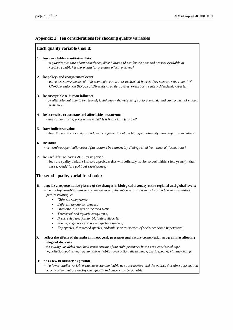
Appendix 2: Ten considerations for choosing quality variables
Each quality variable should:
1. have available quantitative data- is quantitative data about abundance, distribution and use for the past and present available or
reconstructable? Is there data for pressure-effect relations?
2. be policy- and ecosystem-relevant - e.g. ecosystems/species of high economic, cultural or ecological interest (key species, see Annex 1 of
UN-Convention on Biological Diversity), red list species, extinct or threatened (endemic) species.
3. be susceptible to human influence- predictable and able to be steered; is linkage to the outputs of socio-economic and environmental models
possible?
4. be accessible to accurate and affordable measurement- does a monitoring programme exist? Is it financially feasible?
5. have indicative value- does the quality variable provide more information about biological diversity than only its own value?
6. be stable- can anthropogenically-caused fluctuations be reasonably distinguished from natural fluctuations?
7. be useful for at least a 20-30 year period.- does the quality variable indicate a problem that will definitely not be solved within a few years (in that
case it would lose political significance)?
The set of quality variables should:
8. provide a representative picture of the changes in biological diversity at the regional and global levels; - the quality variables must be a cross-section of the entire ecosystem so as to provide a representative
picture relating to:• Different subsystems;• Different taxonomic classes;• High and low parts of the food web;• Terrestrial and aquatic ecosystems;• Present day and former biological diversity;• Sessile, migratory and non-migratory species;• Key species, threatened species, endemic species, species of socio-economic importance.
9. reflect the effects of the main anthropogenic pressures and nature conservation programmes affecting
biological diversity:- the quality variables must be a cross-section of the main pressures in the area considered e.g.:
exploitation, pollution, fragmentation, habitat destruction, disturbance, exotic species, climate change. 10. be as few in number as possible;
- the fewer quality variables the more communicable to policy makers and the public; therefore aggregationto only a few, but preferably one, quality indicator must be possible.

RIVM report 402001014 page 41 of 52
Appendix 3: List of biodiversity indicators for policy makers
(derived from Reid et al., 1993)
Table 6. Indicators of Biodiversity Conservation
Biodiversity conservation Concerns
IndicatorGeneticdiversity
Speciesdiversity
CommunityDiversity
Wild Species and Genetic Diversity
1. Species richness (number, number per unit area, number perhabitat type)
2. Species threatened with extinction (number or percentage)3. Species threatened with extirpation (number or percentage)4. Endemic species (number or percentage)5. Endemic species threatened with extinction (number or
percentage)6. Species risk index7. Species with stable or increasing populations (number or
percentage)8. Species with decreasing populations (number or percentage)9. Threatened species in protected areas (number or percentage)10. Endemic species in protected areas (number or percentage)11. Threatened species in ex-situ collections (number or
percentage)12. Threatened species with viable ex-situ populations (number or
percentage)13. Species used by local residents (number or percentage)
Community Diversity
14. Percentage of area dominated by non-domesticated species15. Rate of change from dominance of non-domesticated species to
domesticated species16. Percentage of area dominated by non-domesticated species
occurring in patches greater than 1,000 sq km17. Percentage of area in strictly protected status
X
XXXX
XX
XXXX
X
X
X
XXXX
XX
XXXX
X
X
XX
X
X
XX
X
X
page 42 of 52 RIVM report 402001014
Appendix 4: Review of existing indicators
The indicators 1-17 from Appendix 3 and nine additional, more recent, indicator proposalsare reviewed on their suitability for integrated environmental assessments, especiallyOECD’s Environmental outlook and Strategy. The suitability is determined according to tenconsiderations as shown in Appendix 2. Only the main advantages and disadvantages arementioned. The numbers 1-17 refer to the number in Table 6 in Appendix 3.
1. Species richness (number, number per unit area, number per habitat type) (Reid et al.,1993)The availability of data is often limited to a few distinct groups such as (some) vertebratesand vascular plants (Reid et al., 1993). Monitoring 'species richness' periodically, coveringthe whole world, would cost a considerable amount of money, even when it is limited to asmall number of groups. The result is a function of the monitoring effort, which makes thetrends less comparable and almost impossible to assess. Furthermore, it is difficult to relatethis indicator with pressures in order to make predictions, because extinction is difficult tomeasure or to predict. Moreover, this has to be done for a large number of species, even whenit is limited to some groups (vertebrates alone consist of ten thousands of species). Speciesrichness depends on the spatial scale considered. The larger the scale, the greater thediversity. When areas differ in size, as is the case when countries or biogeographic areas areused, a coherent comparison between areas is problematic. Species diversity appears to be aslow indicator for biodiversity loss, especially when the area considered become larger.Before a species becomes extirpated or extinct, a long -fatal- process of population declinehas already taken place. Generally this is the case in all regions: the abundance of manyspecies decline while the abundance of some opportunistic species increase. However, thepresence of species at the country or regional level changes at a much lower rate. Species-richness is an expensive, insensitive and barely predictable indicator. Trends may be afunction of monitoring effort. Current data are only available for a few taxonomic groups. Itis a useful indicator to compare areas and identify “hot spots” (spatial component). Species-richness is less useful for showing trends within an area (temporal component).
2/3.Species threatened with extinction or extirpation (number or percentage) (Reid et al.,1993)To date, Red Lists and Red Data Books in general not only reflect those species consideredmost threatened, but also very strongly reflect the process and methodology of assessment(WCMC, 1996). Therefore, it is difficult to track changes over time. Another problem is howto assess a “specific number of threatened species”. Is a high or increasing number a positiveor a negative signal? Species might be re-introduced (increased number of threatened species)or might be extinct (a decreased number). Data are only available of a small number ofspecies. Periodic monitoring will be expensive, even when the group considered is relativelyconfined, such as vertebrates or vascular plants. It is difficult to make predictions, as in“species-richness”. “Threatened species” appear to be politically important often urgingpolicy-makers to take direct action. Threatened species have one biogeographical feature incommon: the existence of low numbers in a given area. As a group they do not provide arepresentative picture of the state and changes in biodiversity as a whole. Threatened speciescan produce direct, clear action to prevent irreversible biodiversity loss by extinction.
4/5. Endemic species, threatened with extinction (number or percentage) (Reid et al., 1993)Endemic species are spatial-scale dependent since all species are endemic to some region.This feature makes this indicator a function of the chosen scale and of extirpation elsewhere.Furthermore, endemic species are a function of monitoring effort, as in “species-richness”.This makes this indicator unstable and trends are hard to assess. As in “species-richness” and

RIVM report 402001014 page 43 of 52
“threatened species”, it is difficult to make predictions based on socio-economic scenarios.“Endemic species” appear to be politically relevant, especially when they are threatened anddistributed in one country. Because of this, the endemic state adds an extra dimension toindicators 2/3. As in threatened species, the number of threatened endemic species does notgive a representative picture of the state of biodiversity. Threatened endemic species do notreasonably reflect main causes of biodiversity change and conservation programmes, and arenot sensitive to trends within areas, as in the above-listed indicators. The number ofthreatened endemic species might be useful to compare areas to set priorities. The selectionof endemic species puts extra political weight on “threatened species” and can thus preventirreversible extinction.
6. Species risk index (Reid et al., 1993)This index combines the number of endemic species per area and the proportion of thenatural area that have been lost. It does not provide an indication of the real risk for specificspecies in the present and future, but ranks/prioritises areas based on the potential number ofendemic species at risk. Only “area loss” is included as pressure: there is no other sort ofpressure. Thus, predictions based on different socio-economic scenarios are of limited value.
7/8. Species (populations) with stable or increasing populations, and with decreasingpopulations (number or percentage) (Reid et al., 1993) Numerical estimations of population sizes are rare, but in many more cases it is possible toestimate whether species are increasing or decreasing (WCMC, 1996). Generally, monitoringpopulations is expensive. It is only affordable when a small number of relatively well-knownand easily measurable species are chosen. When these species are also chosen on the basis oftheir representing changes of biodiversity as a whole, they become ecosystem- and policy-relevant indicators. “Representativeness” is a feature that has yet to be properly underpinnedscientifically. Expert judgement could be used to approximate the choice of a representativeset of indicators. In contrast to ”species-richness”, population changes are space-independent(density), sensitive to change, unambiguously measurable and providing early warning. Forthe selected species, specific measure-effect relations can be set up to base predictions ondifferent socio-economic scenarios. This indicator has been implemented in various cases.Population changes in a representative core set of species are suitable for providing a timelypicture of trends. They are not suitable for comparing biodiversity between areas (“hotspots”).
9/10. Threatened and endemic species in protected areas (number or percentage) (Reid et al.,1993)The “number of threatened or endemic species in protected areas” indicates the potentialconservation role of these areas. They do not provide information about the state ofbiodiversity itself. These indicators are merely response indicators, providing information onconservation measures taken, and are therefore important for making predictions on futurebiodiversity.
11/12. Threatened species maintained in ex-situ collections or viable populations (number orpercentage) (Reid et al., 1993)These indicators are similar to the response indicators mentioned above. They provideinformation needed for making prognoses for the future.
13. Species used by local residents (number or percentage) (Reid et al., 1993)This is an indirect indicator of the state of biodiversity. If changes in species used aredetected, this could indicate not only changes in the biodiversity as such, but also changes inlocal interests, market value etc. Therefore, this indicator is in essence an indicator for directuses, and less suitable as state indicator of biodiversity.

page 44 of 52 RIVM report 402001014
14/15/16. Percentage (and extent) of area dominated structurally by non-domesticatedspecies (in patches greater than 1,000 sq. km), and rate of change (Reid et al., 1993)In general, data are available for this indicator. If the indicator “dominated structurally bynon-domesticated species'” is well-defined it can be easily measured and linked to socio-economic factors and related land use and land cover. It is policy and ecosystem relevantbecause land conversion and ecosystem restoration are main factors of biodiversity loss(gain). This indicator has a high indicative value for biodiversity at the ecosystem level, andis stable because changes are not masked by natural fluctuations. This indicator has nosignificance for freshwater and marine areas.
17. Percentage (extent) of area with strictly protected status (Reid et al., 1993)This indicator does not provide information on the state of the world's biodiversity as such, orthe state within these protected areas. Actually it is a response indicator, providinginformation about the conservation measures taken, and essential for making predictions onthe remaining area and biodiversity in the future. Apart from this, other information onresponses is needed, such as measures for pollution abatement, poaching, water use, grazing,exploitation, fragmentation, etc. to make a prediction on the state of an ecosystem. Thisindicator has been implemented in various cases.
18. Habitat index (Hannah, 1994a, b)The "Habitat index" aims to indicate the extent of area that is either not or only partiallydisturbed by human activities in a specified region using the following equation:
Habitat index = undisturbed area+0.25 (partially disturbed area) x 100 Total area
The level of disturbance is divided into three coarse classes, and is defined as follows.Undisturbed: e.g. primary vegetation and low human population density (maximum personsper km2). Partially disturbed: e.g. secondary vegetation, fixed density ranges of persons andcattle. Human dominated: e.g. permanent agricultural or urban settlement. A high “habitatindex value” indicates domination of natural area, and vice versa.Data appear to be reasonably available at the global level, but changes found after re-assessment might easily be a product of different means of division into the three“disturbance” categories. The coarse classes result in a relatively insensitive indicator. It isrelatively easy to make predictions, e.g. for land conversion by agriculture, urbanisation, andexpected human density and livestock. Other pressures are not clearly incorporated. Theindex is highly aggregated, and easy to understand.The habitat index does provide a coarse picture of the state of biodiversity itself (area and acoarse quality measure), and it is not possible to determine societal consequences as a resultof an increasing or declining habitat index because it is not specific on economic relevantspecies or other relevant ecosystem quality variables. Furthermore, the habitat index assumesfixed disturbance by human activities, so it excludes the possibility of lowering humanimpact of activities by improving techniques and management regimes. These improvementsare important options to be assessed in integrated environmental assessments. This indicatoris not applicable to freshwater and marine areas. The indicator has been implemented on theglobal scale.
19. Keystone species (Paine, 1969)"Keystone species" are frequently mentioned as useful indicators for the ecologicalfunctioning of a community. Their presence is assumed to be crucial in maintaining theorganisation and diversity of their ecological communities. However, the term is poorlydefined and non-specific. It is difficult to say what is and what is not a keystone species

RIVM report 402001014 page 45 of 52
(Scott Mills et al., 1993). Nevertheless, some species have more impact on an ecosystem thanothers because of their biomass, energy transfer or ecosystem shaping and ecosystemstructuring performance (e.g. phytoplankton, large herbivores, trees, coral reefs). Whenchoosing species as indicators it would be favourable to have “key-stone-like” propertiesfrom a representativeness point of view.
20. World Bank/GEF's Natural Capital Indicator (Rodenburg et al., 1995)The Natural Capital Indicator (NCI) is calculated as each country's part of the world's total ofremaining natural areas, adjusted for (multiplied) by its biodiversity richness. Thebiodiversity richness has been defined as the actual number of species (vertebrates andvascular plants) plus the number of endemic species per country. This number is comparedwith the expected "average biodiversity" for a country with a given territory (ratio ofactual/average biodiversity).Data on natural and man-made areas appear to be available, as are data on species richnessand endemics. The NCI ranks the country's current share of the world's biodiversity; it doesnot provide information on the state of biodiversity as such and consequently on possiblesocietal consequences. The remaining natural area factor is easy to link to socio-economicscenarios, so predictions can be made. As indicated above (indicator 1) the species- richnessfactor is hard to predict and insensitive, so is the Natural Capital Indicator as a whole. Theindicator is highly aggregated and concise. The ranking of countries is simple and appealingto policy makers. It is a useful indicator to compare areas and identify "hot spots" (spatialcomponent). It is less useful for showing trends within an area based on socio-economicscenarios within regions (temporal component) . The indicator has been implemented.
21. World Bank’s Natural Capital Indicator (World Bank, 1996)The Natural Capital includes the entire environmental patrimony of a country, expressed inmonetary terms. The elements included are the monetary value of agricultural land, pasturelands, forests, (timber and non-timber products), protected areas, metals and minerals andcoal, oil and natural gas (World Bank, 1996).Data appears to be easily available at the global level. It is relatively easy to makepredictions, given different socio-economic scenarios. However, the indicator omitsbiodiversity of no commercial value. The Natural Capital is changing due to changes in theeconomic market, and not of changes in the actual state of biodiversity. It also contains, to agreat extent, elements which are not relevant for the state of biodiversity, such as subsoilassets. The indicator has been rudimentarily implemented.
22. World Resources Institute’s Ecosystems at Risk indicator (Bryant, 1995; 1997)This method estimates the state of ecosystems as a function of a limited set of main pressures.It is assumed that the higher the (combined) pressures, the higher the risk for the ecosystem.Global assessments have been made of coastal zones and frontier forests, categorising themas being at low, medium or high risk (Bryant, 1995; 1997). It can be seen as a pressure-derived state indicator.Data appear to be easily available at the global level. It is relatively easy to make predictionsgiven different socio-economic scenarios. Furthermore, this indicator reflects importantcauses of biodiversity change. It is highly aggregated and easy to understand.The Risk index does not provide information on the state of biodiversity itself, and it is notpossible to determine societal consequences as a result of an increasing or declining Riskindex. The Risk index also assumes fixed disturbance by human activities, so abatementmeasures, improved techniques or sustainable practices cannot be incorporated. However,integrated environmental assessments aim to show the interactions between human uses andthe state of the environment, and whether a "state of sustainable development" or "sustainableuse" has been reached. It is a very valuable early-warning indicator and could be used as a

page 46 of 52 RIVM report 402001014
substitute as long as no actual state indicators are available. The indicator has beenimplemented at the global level.
23. Biodiversity indicators in OECD development (OECD, 1993-1999)The OECD is still developing biodiversity indicators on pressure, state and response (OECD,1993, 1997, 1998, 1999). The OECD, 1997 draft report proposes the following pressures:“land use change index,” “road density” and ”loss of small-scale elements in farm land.” Asstate indicators the report proposes the "numbers of threatened and extinct species as a shareof assessed species" and “area of key ecosystems.” In recent years indicators on agro-biodiversity were elaborated (OECD, 1998, 1999). The biodiversity of agro-ecosystems isconsidered a function of the size of the system and its quality: “ecosystem quantity” and“ecosystem quality”, respectively. Ecosystem quantity is the extent of the agricultural areaexpressed as percentage of a country’s area. Ecosystem quality can be expressed in variousquality variables such as the abundance of a core set of species, species richness, proportionof semi-natural and uncultivated natural habitats on agricultural land and the extent peragricultural type.The “land use change index” lacks a clear and unambiguous definition and assessmentprinciple (what change is considered good or bad?) as do ”loss of small-scale elements”(what is an “element”?) and “area of key-ecosystems”. For "numbers of threatened andextinct species as a share of assessed species", see above. The agro-ecosystem indicators arevery similar to the Natural Capital Index framework of the Convention on BiologicalDiversity, evaluated in this report. These indicators have been implemented in a several pilotstudies within the OECD (1999).
24. Biodiversity indicators by UN/CSD (UN, 1996)The Indicators of Sustainable Development programme (ISD) provide pressure, state andresponse indicators, as well as indicators for use. Biodiversity-relevant state indicators are:land use change, changes in land condition, satellite-derived vegetation index, land affectedby desertification, forest area change, algae index, and the percentage of threatened andextinct species. Biodiversity-relevant pressure and use indicators are: sustainable use ofnatural resource in mountain areas, wood harvesting intensity, maximum sustained yields forfisheries & current yields, BOD in water bodies, faecal coliform in fresh water, populationstate and growth in coastal zones, domestic consumption of water per capita, discharge of oilinto coastal areas, N and P discharge in coastal zones, total GDP per capita and GDP per km2,use of agricultural pesticides and fertilisers, irrigated percentage of arable land, energy useper km2 of agriculture, emissions of SO2 and NOx, area affected by salination and waterlogging, and area of land contaminated by hazardous wastes.For evaluation of the state indicators see number 2/3. The pressure indicators can be seen as alist of possible, promising indicators. Their usefulness depends on the specific area. Theycould be useful in the way proposed by WRI (see number 22) as a substitute for stateindicators. In that case they must have a known relationship with the chosen state indicatorsand they must be linkable to socio-economic scenarios. These indicators are to beimplemented in the pilot studies of several countries.
25. Biodiversity indicators in Biodiversity Country Study Guidelines (UNEP, 1993)These guidelines provide a comprehensive list of possible indicators providing a detailed pictureof pressures and the state of biodiversity on the local and national scale. In addition, theseguidelines help define the different issues to be dealt with and the structure of reporting. Theydo not aim at standardised, highly aggregated indicators at the regional or global level, and donot fit into a general framework of environmental assessment and modelling. The indicatorshave been implemented in several national pilot studies.

RIVM report 402001014 page 47 of 52
26. Convention on Biological Diversity (UNEP, 1997b, 1999) & Global Biodiversity Forum(GBF, 1997)These reports propose pressure, state, response and use indicators. The pressure and stateindicators are those dealt with in this paper.

page 48 of 52 RIVM report 402001014
Appendix 5: A comparison of major indicator frameworks
Table 7 summarises the main features of the major indicator frameworks (see No. 20-26 inAppendix 4).
Table 7: Major indicator frameworks: main features compared
Frame-works
BiodiversityIndicatorsP - S - R
Use-Indic.
Scale Past/pres/Future
Integr.Framw
IntegratedModelling
Focus onstate/change
Assessmentprinciple
GEO/NCI + + - - All + + + + + + + +WRI-risk + - - - All - + - - - + - +GEF/NCI - + - - Nat - + - - - + - +WB/NCI - monetary - - Nat - + - + - + + +OECD + + + - Nat - + - + - + + -CBD + + - + All + + + + + + + +GBF + + + + All + + + + + + + +Country Gl. + + + - loc/nat - + - - - + - -ISD[?] + + + + Nat - + - + - + - -Legend:P-S-R: pressure, state and response indicatorsscale: local, national, regional, globalintegrated framework: part of integrated environment assessment frameworkintegrated modelling: prognoses possible, linkable to models and socio-economic scenariosstate/change: focus on actual state in absolute terms or the change in relative termsassessment principle: clear choice whether a change is considered positive or negative + : yes, suitable for, designed for, explicit- : no, not designed for, not explicit+ : in some way; low elaboration
In UNEP’s Global Environment Outlook (GEO) the NCI framework does not aim to offer acomprehensive, detailed and entirely representative description of the state of biodiversity on anational or subnational scale. It aims to provide a rough picture of the main changes inbiodiversity from the past and present to the future at the regional and global level, as they areimpacted by socio-economic developments and associated environmental changes.
The ecosystems-at-risk indicator of the World Resource Institute (WRI) is a pressureindicator at the regional and global level. It has been incorporated as a suitable indicator in theGEO/NCI framework.
The Global Environment Facility (GEF)/Natural Capital Indicator is a stateindicator defined at the country level. It is not suitable to link with socio-economic scenarios.
The WorldBank (WB)/Natural Capital Indicator is a state indicator that includes theentire environmental patrimony of a country such as: agricultural land, pasture lands, forestsproducts, protected areas, metals and minerals and coal, and oil and natural gas, expressed inmonetary terms.
The Global Biodiversity Assessment (GBA)(UNEP, 1995) provides a broad overview ofthe current state of scientific knowledge, identifies gaps in knowledge and draws attention toscientific issues where scientists have reached a consensus, as well as to those whereuncertainty has led to conflicting viewpoints. It is not intended to assess the state of thebiodiversity as such for the various ecosystems in the past, present and future.
The OECD is developing biodiversity indicators on pressure, state and response atthe national level. They are still in the making.
RIVM report 402001014 page 49 of 52
The Convention on Biological Diversity (CBD) and Global Biodiversity Forum (GBF)have proposed indicators which are identical to the proposal for GEO/Natural Capital Indexframework (NCI). They are developed in a concerted action.
The Biodiversity Country Study Guidelines provide a kind of comprehensive list ofpossible indicators that can provide a detailed picture of the state of biodiversity on the localand national scale. In addition, these guidelines help define the different issues to be dealt withand the structure of reporting. They do not aim at standardised high aggregated indicators at theregional or global level, and do not fit into a general framework of environmental assessmentand modelling. Several similar indicators are incorporated in the GEO/NCI framework..
The Indicators of the Sustainable Development programme (ISD) provide pressure,state and response indicators, as well as indicators for use. Several indicators areincorporated in the GEO/NCI framework.

page 50 of 52 RIVM report 402001014
Appendix 6: Defining a baseline for natural and man-made habitats
The definition and determination of a baseline corresponding to a more natural, pre-industrialstate, or close to it, is the most challenging part of the framework. Nevertheless, if it were leftout of the framework it would create new problems. The use of a less modified, “pre-industrial baseline" has three major advantages. First, it provides a fair and commoncalibration point to compare the current biodiversity, so policy-makers and the public can getan idea of the major (predominantly anthropogenic) changes which have already taken placein modern, industrial times. This point in time will be different from place to place, and fromstate to state, but it is a comparable point for all nations in their socio-economic developmentand the resulting high modification of “natural” ecosystems and traditional, highly diverse,agricultural landscapes. Second, it provides the possibility to assess whether any change inbiological diversity since the start of the CBD agreement is good or bad from biodiversityconservation perspective. This is possible despite the possible absence of verifiableecological objectives. The third reason is that a baseline point enables us to remove the unitsof the many different biodiversity variables and make indices: distance to reference (dtr).This allows us to aggregate many different biodiversity parameters to a few or perhaps asingle, more or less representative biodiversity (quality) index for entire ecosystems. This isanalogous to the GNP and Price Index as highly aggregated indicators for the state of theentire economy, consisting of figures from many different economic activities and pricechanges. The health of a person is also assessed using several health variables related tobaseline values.
Assuming that a more natural baseline state has a crucial function in the assessmentof biodiversity, the question arises on how to deal with the theoretical and practicaldifficulties . Pristine or non-human affected ecosystems no longer exist, because humanshave been part of most ecosystems for the last 100,000 years. We know today that even inprehistoric times humans had a considerable effect. Many, large animals and forest systemshave been exploited to extinction. The human’s impact (per time unit) was low in early times,and has gradually increased with growing technology, population, production andconsumption rates in modern times. Biodiversity is currently decreasing at an unprecedentedhigh rate (see the Global Biodiversity Assessment, 1995). It is this unprecedented rapidchange in modern times that we want (and are obliged) to show quantitatively in national,regional and global assessment reports. Since there is no unambiguous natural reference pointin history, and all ecosystems are also transitory by nature, a baseline point must beestablished at an arbitrary but practical point in time. There is nothing wrong in this, providedthe arbitrariness of the baseline is acknowledged and commonly applied.
Because it makes most sense to show the biodiversity change when human influencewas accelerating rapidly, the baseline should preferably be just before modern times: a pre-industrial state. This choice means that pre-industrial human influences are part of thebaseline. For every region, nation or location this point in time may be different. Also, theavailability or reconstructability of data will play a role in this choice. Data availability willgenerally increase as time progresses, so in some cases the baseline must be set in (early)industrial times. It is up to countries to choose this point. Once the baseline has been chosen,it has to be used consistently over time, so that trends can be quantified unambiguously.
Given the above, it is proposed to use the concept "postulated baseline, set in pre-industrial times", or in short, the "postulated baseline." For heavily modified, man-madeagricultural ecosystems, the often biodiversity-rich, traditional-agricultural ecosystem isapplied as the baseline.
Parties will most probably identify baseline ranges for the differentvariables/indicators utilised. These ranges are subject to revision pending availability of newdata and insights. This also requires adjustment of the assessment figures in the past to enablecomparison over time. To enable aggregation of data up to regions and globally, thesebaselines should be internationally discussed. Major differences, which are initiallyinevitable
RIVM report 402001014 page 51 of 52
between countries, could be harmonised in the longer term, as has also been the case (andstill is) with economic indicators.

page 52 of 52 RIVM report 402001014
Appendix 7: Specification of natural and man-made ecosystems
Man-made ecosystems:Heavily modified areas intensively used by humans such as:• Built-up area• cropland• planted pasture for permanent livestock• infrastructure• industrial and mining area• planted forest with exotic species• channels, ditches, man-made reservoirs & mariculture ponds• self- regenerating patches < 100 ha. Natural ecosystems: All other primarily natural and semi-natural areas, possibly extensively used ecosystems,irrespective of their ecological quality, larger than 100 ha., such as:• nature area• extensively used areas, such as shifting cultivation areas, areas with nomadic
livestock and areas with indigenous people living in a traditional way• all forest (including production forest, except for forest planted with exotic species)• rangeland of native pastures• all fresh water, except for channels, ditches, man-made reservoirs & mariculture
ponds• marine area