research article soil water flow patterns due to distance

Horticultural Science and Technology 631

Received: April 20, 2020

Revised: June 26, 2020

Accepted: June 27, 2020

OPEN ACCESS

HORTICULTURAL SCIENCE and TECHNOLOGY

38(5):631-644, 2020

URL: http://www.hst-j.org

pISSN : 1226-8763

eISSN : 2465-8588

This is an Open Access article distributed

under the terms of the Creative Commons

Attribution Non-Commercial License which

permits unrestricted non-commercial use,

distribution, and reproduction in any medium,

provided the original work is properly cited.

Copyrightⓒ2020 Korean Society for

Horticultural Science.

This work was supported by the Rural Deve-lopment Administration (RDA) (Project No. PJ01228704).

RESEARCH ARTICLE https://doi.org/10.7235/HORT.20200058

Soil Water Flow Patterns due to Distance of Two Emitters of Surface Drip Irrigation for Horticultural Crops

Soon Hong Kwon1†

, Dong Hyun Kim1†

, Jong Soon Kim1*

, Ki Yeol Jung2,

Sang Hun Lee2, and Joon Kook Kwon

3

1Department of Bio-industrial Machinery Engineering, Pusan National University, Korea

2Crop Production Technology Division, National Institute of Crop Science, Korea

3National Institute of Horticultural and Herbal Science, Korea

*Corresponding author: [email protected]

†These authors contributed equally to this work.

Abstract

Surface drip irrigation is one of the most efficient systems for irrigating vegetables. The patterns of

soil water distribution formed under the emitter are important for designing an optimal drip irrigation

system. This study aims to evaluate the soil water patterns between two emitters using field

experiments and numerical simulations. Field experiments were conducted using two emitters with

different lateral spacings (20, 40, and 60 cm). Frequency domain reflectometry (FDR) sensors were

used to measure the soil water content. HYDRUS-2D software was used to simulate water

infiltration in the field experiments. At a short lateral spacing (20 cm), the water content started to

increase at 30 min and saturated at 200 min. These values became significantly larger as the lateral

spacing increased—300 min and saturated at 700 min at 40 cm and 900 min and longer than 22

hours at 60 cm, respectively. The simulated water contents were in satisfactory agreement with the

experimental values (R2 = 0.97, RMSE = 0.009 cm

3 cm

-3, E (coefficient of efficiency) = 0.959).

These results provide valuable information that can be used to design an efficient surface drip

irrigation system for vegetables, thereby improving crop productivity and quality.

Additional key words: emitter spacing, field experiment, numerical model, vegetables, water infiltration

Introduction

Surface drip irrigation is one of the most efficient methods for irrigating vegetables. Because it

releases small amounts of water at a high frequency, the water use efficiency is higher. Many

researchers have reported high yields and quality of vegetable crops using surface drip irrigation—

potato (Wang et al., 2006), eggplant (Colak et al., 2018), cucumber (Yuan et al., 2006), and bell

pepper (Sezen et al., 2006). Surface drip irrigation uses emitters and lateral lines laid on the soil

surface. An emitter discharges small amounts of water at a controlled rate, and water infiltration

occurs in the soil region directly around the emitter. Thus, the soil water content in the plant root zone

632 Horticultural Science and Technology


remains essentially constant. Emitters with close spacing (0.1 ‑ 0.6 m) are frequently used for irrigation of small fruits and

vegetables.

Because many farmers use surface drip irrigation, increasing water use efficiency in irrigation is crucial. Realizing the

full potential of drip irrigation technology requires optimization of operational parameters, which are the rate of discharge

from the emitter, emitter spacing, duration of water application, and placement of drip tubing (Skaggs et al., 2004). In

addition, the soil water distribution patterns formed under the emitter are important for designing an optimal drip

irrigation system. Numerical simulations of water transport in unsaturated soils have been used extensively owing to the

complexity of the coupling of water and heat transport in soils and the difficulties associated with field measurements,

especially near the soil surface. HYDRUS-2D can simulate three-dimensional water flow, solute transport, and root water

uptake based on finite-element methods of the flow equations (Šimůnek et al., 2012). This program is effective for

analyzing design features and managing drip irrigation (Cote et al., 2003; Schmitz et al., 2002). However, the simulation

must be compared with experimental results to establish its reliability and to evaluate the physical assumptions involved.

Many experiments and simulations have been conducted on water flow in soil to evaluate the efficiency irrigation

systems. Arraes et al. (2019) developed a numerical model that simulates the water distribution and the shape of the

wetted soil. However, this research only used a point source as the soil surface dripper. Zhang et al. (2012) measured

differences in wetting patterns between a point source and a line source. Some studies using software or experiments have

included soil wetting patterns formed during surface drip irrigation (Kandelous and Šimůnek, 2010; Kandelous et al.,

2011; Samadianfard et al., 2012; Dabach et al., 2013; Autovino et al., 2018). Although surface drip irrigation has been

studied extensively, to our knowledge, no analysis of wetting patterns when using different emitter spacings for

horticultural crops has been conducted. Therefore, this study simulates the wetting patterns in surface drip irrigation using

the numerical HYDRUS-2D model, compares the values with the experimental data, and assesses the use of simulation in

a design drip management system for horticultural crops. This study was carried out using three lateral line spacings (i.e.,

20, 40, and 60 cm).

Materials and Methods

Experimental Setup and Measurements

The experimental site (35°29’N, 128°44’E, 14-m altitude) is located at the Department of Southern Area Crop Science,

National Institute of Crop Science, Republic of Korea. Each experimental plot, 2 × 2 m square, was originally used as a

lysimeter. Table 1 shows the physicochemical properties of the soil studied. The soil texture in this experiment was sandy

loam (sand 61.5%, silt 30.5%) (Kim et al., 2018), which quickly drains excess water. Most vegetables grow well in sandy

loam soil.

Table 1. Physico-chemical properties of soil

Soil texturepH

(1:5)

EC

(dS·m-1)

T-N

(%)

O.M.

(g·kg-1)

Avail. P2O5

(mg kg-1)

Exch. Cation (cmolc·kg-1) Particle size (%)

K Ca Mg Sand Silt Clay

Sandy loam 6.44 0.43 0.27 26.5 264.8 1.75 14.97 4.5 61.5 30.5 8.0



Fig. 1. Location of the emitters and FDR probe at a dripline spacing of 20 cm in the experimental plot.

The wetting patterns of two neighboring emitters eventually overlap to some extent, depending on the emitter spacing.

These patterns are also affected by the initial water content and soil properties. However, because the emitter spacing was

fixed at 20 cm, the dripline spacing was varied to evaluate the movement of irrigated water between the emitters. As a

result, the spacings between two lateral driplines were 20, 40, and 60 cm, which are the common distances for drip

irrigation of fruits and vegetables. The emitter discharge rate and the soil texture were 2.1 L/h and sandy loam,

respectively.

Soil water content was measured using a frequency domain reflectometry (FDR) sensor (EnviroPro, Entelechy, Australia).

This sensor monitors the changes in the dielectric properties of the soil to provide soil moisture. The sensor was installed

in accordance with the manufacturer's installation manual to increase the accuracy of the measured values. Any

disturbance of soil adjacent to the probe will affect the measurement accuracy. Thus, we confirmed that there were no air

gaps or preferential water flow along the probe during the experiment. These 40-cm-long soil probes were installed in the

middle of the emitters at adjacent driplines (Fig. 1). The sensors in the soil probe were located at 10-cm increments

vertically from the soil surface, i.e., at depths of 10, 20, 30, and 40 cm. This probe was also connected to a data logger,

which was programmed to save the data every 10 min. The measured value was adjusted to the value that corresponded

to sandy loam soil according to the calibration equation provided by the manufacturer. The measurement accuracy of soil

moisture was ± 2%, according to the manufacturer’s manual. In addition, the probes were calibrated for the experimental

site by the manufacturer.

In this experiment, a single multi-sensor was used to measure the distribution of soil water. In general, in order to

measure water content profiles in the field, several TDR probes were installed vertically or horizontally (Ferre and Topp,

2002; Ramos et al., 2012). By contrast, our FDR probe provided the water content profile from a single installation. Since

our study was focused on water infiltration, one sensor for each condition was enough to compare the simulation data;

once the discrete measuring data were close to the simulation values, the real water distribution would be similar to the

simulation distribution.

This experiment was carried out from 11:00 a.m. on November 6, 2019 to 9:00 a.m. on November 7, 2019 (22 h).

Weather data were collected from an automated weather station in the experimental field, and the average temperature and

relative humidity were 11°C and 77.1%, respectively. All experiments in this study were performed in triplicate.



Simulation

HYDRUS-2D Model

HYDRUS-2D software (Šimůnek et al., 2012) was used to simulate the two-dimensional movement of water in the soil.

Water flow was described using the Richards equation (Richards, 1931).

, (1)

where θ is the volumetric water content (cm3 cm-3) in the soil; h is the pressure head (cm); K is the hydraulic conductivity

(cm min-1); x and z are the horizontal and vertical coordinates (cm), respectively; t is time (min); and S is the sink term

(min-1).

This partial-differential equation governs variably saturated flow in the unsaturated zone. The soil water retention curve

and the unsaturated hydraulic conductivity function K(h) were calculated using the van Genuchten ‑ Mualem

constitutive relationships (Van Genuchten, 1980).

, (2)

, (3)

where and are the saturated and residual water contents (cm3 cm-3), respectively; (cm-1), n ( ‑ ), and m (=1 ‑ 1/n) (‑)

are empirical parameters; Ks is the saturated hydraulic conductivity (cm min-1); and l is the pore connectivity parameter.

Se, the degree of saturation, is expressed by the following equation:

(4)

The Richards equation is a nonlinear partial-differential equation. The coefficient of K(h) is a function of the dependent

variable . Because of its strong nonlinearity, most practical applications of the Richards equation require a numerical

solution.

Simulation Conditions and Parameters

Because the drip tubing had the same emitter spacing (20 cm) and the water was only supplied from the emitters, the

emitter was considered a point source. In general, the emitter flux is much greater than the saturated hydraulic

conductivity, so the infiltration zone becomes saturated quickly. Therefore, the water flow is symmetrical about the

vertical centerline of the emitter. Hence, the soil water distribution patterns at different lateral (drip tubing) spacings

would be the same as those at different emitter spacings.

Fig. 2 shows the dimensions in the simulations: the domain was 100 cm wide and 100 cm deep. The Richards equation



Fig. 2. Boundary conditions and observing node locations used in HYDRUS-2D simulations.

can be solved numerically with specific initial and boundary conditions. The initial conditions characterize the initial state

of the system and are specified in terms of the water content in the vertical direction.

, (5)

where (cm3 cm-3) is the initial value of the water content. These initial conditions were uniform in the horizontal

direction. The initial conditions were based on the measured data.

At the soil surface, one must account for interactions between the applied water rate and evaporation.

at t > 0, z = 0, x > 0, (6)

where is the initial flux (cm min-1), Q is the emitter flow rate (cm min-1), and Ea is the actual evaporation rate (cm min-1).

At both lateral boundaries, there was a no-flow condition to account for flow and transport symmetry.

for t > 0, z > 0 (7)

Here, Jw is the water flux (cm min-1), Ks is the hydraulic conductivity (cm min-1), and H is the total head (cm).

At the bottom of the soil profile, there is a free drainage condition.



Table 2. Properties of soils considered in HYDRUS-2D simulations

Soil type

(cm-1) Ks (cm/min) l

Surface soil 0.13 0.5 0.38 2.2 0.15 0.5

Subsoil 0.23 0.5 0.37 2.16 0.136 0.5

, (8)

where go is the prescribed total gradient (cm cm-1). This boundary condition is commonly used when the water table is

situated far below the domain of interest.

The soil hydraulic parameters (Table 2) were estimated using the ROSETTA pedotransfer function of Schaap et al.

(2001), as implemented in the HYDRUS code. Soil hydraulic properties vary among soils with a textural class. This is

especially true near the soil surface, which is affected more by land use and weather (Radcliffe and Šimůnek, 2010). Thus,

the soil region was also divided into the surface soil (0 ‑ 15-cm depth) and the subsoil (15 ‑ 100-cm depth). The hydraulic

conductivity at the soil surface was higher than that at the subsoil because of the larger porosity in the soil surface region.

The emitters were located on the surface, and their discharge rate was 2.1 L/h. Observation nodes were set to a 40-cm

depth by increments of 10 cm from the surface (10, 20, 30, and 40 cm). Because the FDR probe was installed in the middle

of the emitters, the observing dimension of each node group was set to 6 cm (horizontal direction) by 5 cm (vertical

direction) to cover a dielectric-affected area from the FDR sensor. Simulations were performed with three dripline

spacings (20, 40, and 60 cm) to investigate the soil water distribution for different drip tube spacings. The soil type was

sandy loam in the simulations. The irrigation time in the simulation was 22 h, which is the same as the field experiment,

to compare the simulated values with the measured ones.

Statistical Analysis

Statistical tests were employed on the measured and simulated data generated from the field experiment and modeling.

The model’s performance was evaluated by comparing measured (M) and HYDRUS-2D simulated (S) values of soil

water content. The error between these values was estimated using the root mean square error (RMSE), given by

∑

(9)

The coefficient of determination (R2) was also applied to test the proportion of variance in the measured data explained

by the model. In addition, the coefficient of efficiency (E) was used to evaluate the performance of the simulation model.

The coefficient of efficiency was defined as one minus the ratio of the mean square error to the variance in the observed

data (Nash and Sutcliffe, 1970).

∑ ̅

∑

(10)



Fig. 3. Comparison of measured and simulated values of the soil water content at a drip tube spacing of 20 cm.

Results and Discussion

Fig. 3 shows the soil water contents at a 20-cm drip tube spacing and a comparison of these values with the

HYDRUS-2D simulation. Because the distance between the emitter and the soil water sensor was relatively close (only

10 cm), the water content at a 10-cm depth began to increase 30 min after the start of irrigation and saturated at almost 200

min. As the sensing points became deeper, the reaching times increased linearly: 50 min at 20 cm, 80 min at 30 cm, and

110 min at 40 cm (Fig. 3). Fig. 4 shows the soil water distributions with irrigation time. The wetting patterns of the two

adjacent emitters began to overlap at 150 min. As the irrigation time increased, they mutually interacted and moved

downward predominantly.

All the initial water contents, except at a 10-cm depth, were 29.0%, and the saturated water content was 43.9%, which

is in the range of saturation water content of sandy loam soil (Soil Water Characteristics, Version 6.02.74, USDA ARS).

However, at a 10-cm depth, the initial water content (21.8%) and the saturation water content (37.0%) were much lower

than at other depths. This experiment was carried out using lysimeters 1 month after harvesting soybeans. Thus, because

of the high organic matter content, the bulk density was low, so the saturation water content was significantly low. In

addition, the sensor placed at a 10-cm depth showed lower values than the simulation (Fig. 3). This could have resulted

from poor contact between the sensor and the soil from a lower bulk density. As a result, at this depth, RMSE, one of the

error measures, was the largest among the depths. Conversely, R2 and E, the regression and efficiency measures, were the

lowest (Table 3). However, the overall values (R2 = 0.948; RMSE = 0.011 cm3 cm-3; E = 0.946) showed satisfactory

agreement between the measured and simulated data. In summary, irrigation with a drip tube spacing of 20 cm is effective

for crops because it can provide water for the crop root zone for less than half an hour. However, in real cultivation, such

a redistribution would be limited because of the crop’s soil water extraction.

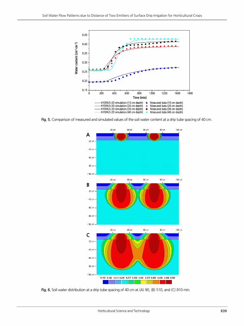
At a drip tube spacing of 40 cm, the emitter’s water took more time to reach the depths than the case with a drip tube

spacing of 20 cm. In addition, the increasing rates (∆∆) were much slower than at a drip tube spacing of 20 cm (Fig.

5). This is attributed to the higher elongation in the vertical direction compared with the horizontal direction (Fig. 6). Both

wetting patterns were not met until 510 min, which is far slower than the time at the drip tube spacing of 20 cm



(approximately 150 min). The wetting pattern continued to increase, and the wetting front reached the bottom at 960 min.

Similar to the drip tube spacing of 20 cm, the initial and saturation water contents at a depth of 10 cm were much lower

than at the deeper ones. However, the saturation water contents at 20, 30, and 40 cm were not the same; this inconsistency

may have been caused by inhomogeneity of soil characteristics along the vertical direction.

A

B

C

Fig. 4. Soil water distribution at the drip tube spacing of 20 cm at (A) 90, (B) 150, and (C) 210 min.

Table 3. Statistical comparison of measured and simulated data at dripline spacing of 20 ,40, and 60 cm

Dripline spacing ParameterSensor depth

10 cm 20 cm 30 cm 40 cm 10 ‑ 40 cm

20 cm

R2

0.753 0.992 0.969 0.973 0.948

RMSE 0.012 0.003 0.007 0.008 0.011

E 0.701 0.979 0.967 0.967 0.946

40 cm

R2

0.968 0.971 0.993 0.984 0.989

RMSE 0.005 0.008 0.005 0.009 0.008

E 0.948 0.970 0.988 0.977 0.988

60 cm

R2

0.968 0.971 0.993 0.984 0.989

RMSE 0.005 0.008 0.005 0.009 0.008

E 0.948 0.970 0.988 0.977 0.988




A

B

C

Fig. 6. Soil water distribution at a drip tube spacing of 40 cm at (A) 90, (B) 510, and (C) 810 min.




In addition, for all depths, the regression analysis (R2 = 0.989) and efficiency testing method (E = 0.988) indicated that

the model accurately predicted the soil water content at a dripline spacing of 40 cm (Table 3). The error parameter (RMSE

= 0.008) also remained within an acceptable limit.

At a drip tube spacing of 60 cm, the soil water content curves at all depths were somewhat different from those for the

preceding spacing (Fig. 7). At depths of 20, 30, and 40 cm, the increasing rates of soil water content (∆∆) were

slowest, and the soil water contents continued to increase until the end of irrigation. This may be because of the elongation

in the vertical direction and the relatively long distance (30 cm) between the emitter and the soil water sensor (Fig. 8). Both

wetting patterns were observed at 900 min.

Similar to other drip tube spacings, at 10-cm depth, the soil water contents were low, and they showed almost constant

values during the irrigation period. Water released from the emitter moved more vertically so that a small amount of water

reached the region. In the simulation, the water contents decreased slightly by 500 min and then increased steadily. In the

surface region, water tends to move downward because of gravity. The surface was also assumed in the model of a

constant atmospheric boundary flux during time steps, which deviates from actual conditions at the surface boundary—

that is, evaporation peaks in the daytime and decreases during the night (Ramos et al., 2012). R2 for the 10-cm depth was

0.837, which was lower than the other depths (Table 3). Conversely, E for a 10-cm depth was also −2.831, which

indicates unacceptable performance (Moriasi et al., 2007). It can be concluded that the poorer correspondence between

simulations and measurements at a 10-cm depth was most likely caused by the inadequacy of the soil hydraulic

parameters. The performance parameters of other depths showed satisfactory agreement between measurements and

simulations.

Drip tube spacing is one of the factors affecting vegetable growth. At a drip tube spacing of 20 cm, all soil depths were

saturated with water within 200 min, which makes it possible to irrigate at the right time during the crop growing season.

There was enough water in the root zone to be taken in by plant roots. However, at a drip tube spacing of 60 cm, irrigation

water was less likely to contribute to the increase in water content midway between the emitters. However, plant

development could not be particularly affected because the water content did not decrease. The effects of a dripline



Fig. 8. Soil water distribution at a drip tube spacing of 60 cm at (A) 90, (B) 720, and (C) 1,320 min.

spacing of 40 cm were between those of 20- and 60-cm spacings.

For all drip tube spacings, R2 of 0.971, RMSE of 0.009 cm3 cm-3, and E of 0.959 were found between the measured and

simulated water contents. Deviations between measured and simulated water contents can be attributed to field

measurements and model input errors.

The source of error in field measurements is related to FDR measurements. FDR probes measure spatially averaged

water contents over a certain soil volume, while simulation provides water content for a precise soil location (Ferre et al.,

2002). Although the observation points (6 × 5 cm) were set at each depth to cover the area, this was not sufficient to

represent highly nonuniform distribution areas, such as a depth of 10 cm. A wider area would give more representative

values.

Another source of error in simulation is the uncertainty of soil hydraulic properties, which were taken from

HYDRUS-2D. A nominal soil profile may not reflect the much larger simulated flow domain under experimental

conditions. Moreover, the spatial and temporal variability of soil hydraulic properties was not considered in the

simulation. Soil evaporation, which is an important factor in water flow simulation, also needs to be adjusted to



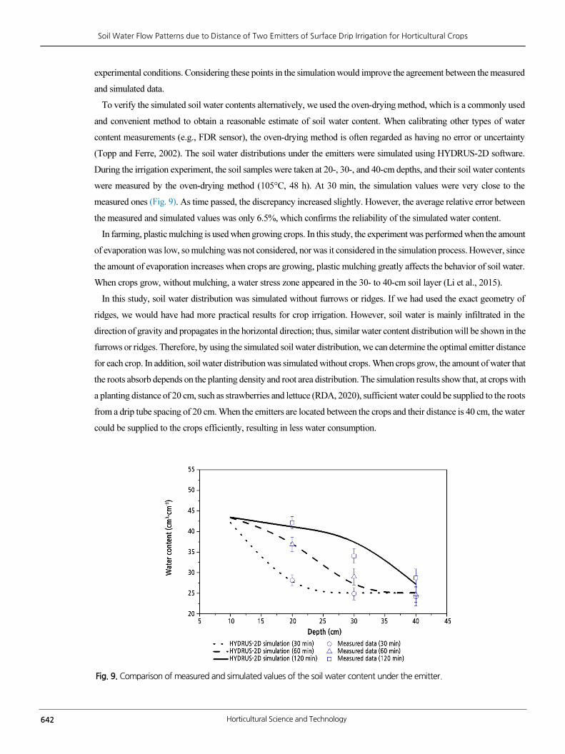
Fig. 9. Comparison of measured and simulated values of the soil water content under the emitter.

experimental conditions. Considering these points in the simulation would improve the agreement between the measured

and simulated data.

To verify the simulated soil water contents alternatively, we used the oven-drying method, which is a commonly used

and convenient method to obtain a reasonable estimate of soil water content. When calibrating other types of water

content measurements (e.g., FDR sensor), the oven-drying method is often regarded as having no error or uncertainty

(Topp and Ferre, 2002). The soil water distributions under the emitters were simulated using HYDRUS-2D software.

During the irrigation experiment, the soil samples were taken at 20-, 30-, and 40-cm depths, and their soil water contents

were measured by the oven-drying method (105°C, 48 h). At 30 min, the simulation values were very close to the

measured ones (Fig. 9). As time passed, the discrepancy increased slightly. However, the average relative error between

the measured and simulated values was only 6.5%, which confirms the reliability of the simulated water content.

In farming, plastic mulching is used when growing crops. In this study, the experiment was performed when the amount

of evaporation was low, so mulching was not considered, nor was it considered in the simulation process. However, since

the amount of evaporation increases when crops are growing, plastic mulching greatly affects the behavior of soil water.

When crops grow, without mulching, a water stress zone appeared in the 30- to 40-cm soil layer (Li et al., 2015).

In this study, soil water distribution was simulated without furrows or ridges. If we had used the exact geometry of

ridges, we would have had more practical results for crop irrigation. However, soil water is mainly infiltrated in the

direction of gravity and propagates in the horizontal direction; thus, similar water content distribution will be shown in the

furrows or ridges. Therefore, by using the simulated soil water distribution, we can determine the optimal emitter distance

for each crop. In addition, soil water distribution was simulated without crops. When crops grow, the amount of water that

the roots absorb depends on the planting density and root area distribution. The simulation results show that, at crops with

a planting distance of 20 cm, such as strawberries and lettuce (RDA, 2020), sufficient water could be supplied to the roots

from a drip tube spacing of 20 cm. When the emitters are located between the crops and their distance is 40 cm, the water

could be supplied to the crops efficiently, resulting in less water consumption.



Rockwool, a fibrous medium, and peat-based substrate mixtures have been widely used for plant cultivation as soilless

substrates. Recently, the water movement characteristics of rockwool were investigated through an irrigation experiment

(Choi and Shin, 2019) and the transpiration rate of paprika cultivated on rockwool was estimated by artificial neural

networks (ANNs) (Nam et al., 2019). In addition, the flowers, petunia and zinnia, were grown in peat-based substrates

with a high or low irrigation level, and their growth performances were analyzed by their irrigation levels (Choi et al.,

2019). However, there aren’t studies available in scientific literature about the water distribution in soilless substrates.

Therefore, the simulation model of water transport in soilless substrates along with the experiment, just like the approach

in this study, would be helpful for developing an appropriate irrigation strategy.

Conclusions

Field experiments were performed to evaluate the water contents with different drip tube spacings when the wetting

fronts were initially separated and later overlapped with time. The water contents were simulated continuously during the

field experiment and compared well with measured experimental data, having an R2 of 0.97, RMSE of 0.009 cm3 cm-3,

and E of 0.959. However, these values indicate much better performance than those from other simulation studies (Skagg

et al., 2004; Kandelous and Šimůnek, 2010). This can be ascribed to the relatively simple simulation conditions, such as

a short irrigation period, no root water uptake, and constant atmospheric boundary water flux. Under field conditions with

surface drip irrigation, patterns of soil water content depend not only on drip tube spacing but also on the soil texture and

emitter discharge rate. The latter, not examined in this study, could be evaluated by using model simulations, such as

HYDRUS-2D.

Drip irrigation is an efficient method of applying water to horticultural crops. Irrigation scheduling is the process of

determining how often to irrigate and how much water to apply. The main goal of irrigation is to provide the crops with

the appropriate amount of water at the exact location, and precise soil water distribution can be obtained by simulation,

which is difficult to perform using only field measurements. Once a simulation procedure is established using the field

data, the modeling approach helps farmers adopt better irrigation management practices. In summary, this simulation

approach using HYDRUS-2D was found to be a useful tool for simulating water infiltration in surface drip irrigation.

However, three-dimensional simulation provides more realistic results.

Literature Cited

Arraes FD, Miranda JHD, Duarte SN (2019) Modeling soil water redistribution under surface drip irrigation. Eng Agríc 39:55-64.

doi:10.1590/1809-4430-eng.agric.v39n1p55-64/2019

Autovino D, Rallo G, Provenzano G (2018) Predicting soil and plant water status dynamic in olive orchards under different irrigation

systems with Hydrus-2D: Model performance and scenario analysis. Agric Water Manag 203:225-235. doi:10.1016/j.agwat.2018.

03.015

Choi S, Xu L, Kim H (2019) Influence of physical properties of peat-based potting mixes substituted with parboiled rice hulls on plant

growth under two irrigation regimes. Hortic Environ Biotechnol 60:895-911. doi:10.1007/s13580-019-00179-9

Choi YB, Shin JH (2019) Analysis of the changes in medium moisture content according to a crop irrigation strategy and the medium

properties for precise moisture content control in rock wool. Hortic Environ Biotechnol 60:337-343. doi:10.1007/s13580-019-0013

4-8

Colak YB, Yazar A, Gonen E, Eroglu EC (2018) Yield and quality response of surface and subsurface drip-irrigated eggplant and



comparison of net returns. Agric Water Manage 206:165-175. doi:10.1016/j.agwat.2018.05.010

Cote CM, Bristow KL, Charlesworth PB, Cook FJ, Thorburn PJ (2003) Analysis of soil wetting and solute transport in sub-surface trickle

irrigation. Irrig Sci 22:143-156. doi:10.1007/s00271-003-0080-8

Dabach S, Lazarovitch N, Šimůnek J, Shani U (2013) Numerical investigation of irrigation scheduling based on soil water status. Irrig Sci

31:27-36. doi:10.1007/s00271-011-0289-x

Ferre PA, Topp CG (2002) Time domain reflectometry. In JH Dane, CG Topp, eds, Methods of Soil Analysis, Part 4. Physical Methods. Soil

Science Society of America, Madison, WI, USA, pp 434-446

Ferre TPA, Nissen HH, Šimůnek J (2002) The effect of the spatial sensitivity of TDR on inferring soil hydraulic properties from water

content measurements made during the advance of a wetting front. Vadose Zone J 1:281-288. doi:10.2136/vzj2002.2810

Kandelous MM, Šimůnek J (2010) Comparison of numerical, analytical, and empirical models to estimate wetting patterns for surface

and subsurface drip irrigation. Irrig Sci 28:435-444. doi:10.1007/s00271-009-0205-9

Kandelous MM, Šimůnek J, Van Genuchten MT, Malek K (2011) Soil water content distributions between two emitters of a subsurface

drip irrigation system. Soil Sci Soc Am J 75:488-497. doi:10.2136/sssaj2010.0181

Kim DH, Choi JY, Kwon SH, So JD, Kwon SG, Chung KY, Lee SH, Kim JS (2018) Water use efficiency of soybean, sorghum, sesame with

different groundwater levels using lysimeter. Korean J Soil Sci Fert 51:339-352. doi:10.7745/KJSSF.2018.51.4.339

Li X, Shi H, Šimůnek J, Gong X, Peng Z (2015) Modeling soil water dynamics in a drip-irrigated intercropping field under plastic mulch.

Irrig Sci 33:289-302. doi:10.1007/s00271-015-0466-4

Moriasi DN, Arnold JG, Van Liew MW, Bingner RL, Harmel RD, Veith TL (2007) Model evaluation guidelines for systematic quantities of

accuracy in watershed simulations. T ASABE 50:885-900. doi:10.13031/2013.23153

Nam DS, Moon T, Lee JW, Son JE (2019) Estimating transpiration rates of hydroponically-grown paprika via an artificial neural network

using aerial and root-zone environments and growth factors in greenhouses. Hortic Environ Biotechnol 60:913-923.

doi:10.1007/s13580-019-00183-z

Nash JE, Sutcliffe JV (1970) River flow forecasting through conceptual models Part I - A discussion of principles. J Hydrol 10:282-290.

doi:10.1016/0022-1694(70)90255-6

Radcliffe DE, Šimůnek J (2010) Soil Physics with HYDRUS - Modeling and Applications. CRC Press, Boca Raton, FL, USA, pp. 85-128

Ramos TB, Šimůnek J, Goncalves MC, Matins JC, Prazeres A, Pereira LS (2012) Two-dimensional modeling of water and nitrogen fate

from sweet sorghum irrigated with fresh and blended saline waters. Agric Water Manag 111:87-104. doi:10.1016/j.agwat.2012.

05.007

Richards LA (1931) Capillary conduction of liquids through porous mediums. Physics 1:318-333. doi:10.1063/1.1745010

Rural Development Administration (RDA) (2020) Crop Production Manual. Rural Development Administration. http://www.nongsaro.

go.kr/ Accessed 01 June 2020

Samadianfard S, Sadraddini AA, Nazemi AH, Provenzano G, Kisi O (2012) Estimating soil wetting patterns for drip irrigation using genetic

programming. SPAN J Agric Res 4:1155-1166. doi:10.5424/sjar/2012104-502-11

Schaap MG, Leij FJ, van Genuchten MT (2001) ROSETTA: A computer program for estimating soil hydraulic properties with hierarchical

pedotransfer functions. J Hydrol 251:163-176. doi:10.1016/S0022-1694(01)00466-8

Schmitz G, Schutze N, Petersohn U (2002) New strategy for water application under trickle irrigation. J Irrig Drain Eng 128:287-297.

doi:10.1061(ASCE)0733-9437(2002)128:5(287)

Sezen SM, Yazar A, Eker S (2006) Effect of drip irrigation regimes on yield and quality of field grown bell pepper. Agric Water Manag

81:115-131. doi:10.1016/j.agwat.2005.04.002

Šimůnek J, Van Genuchten MT, Šejna M (2012) The HYDRUS software package for simulating two- and three-dimensional movement

of water, heat, and multiple solutes in variably-saturated media. Technical Manual, Version 2. PC Progress, Prague, Czech Republic

Skaggs TH, Trout TJ, Šimůnek J, Shouse PJ (2004) Comparison of HYDRUS-2D simulations of drip irrigation with experimental observations.

J Irrig Drain E 130:304-310. doi:10.1061/(ASCE)0733-9437(2004)130:4(304)

Topp CG, Ferre PA (2002) Theromogravimetric Using Convective Oven-Drying. In JH Dane, CG Topp, eds, Methods of Soil Analysis. Part

4. Physical Methods. Soil Science Society of America, Madison, WI, USA, pp 422-424

Van Genuchten MT (1980) A closed-form equation for predicting the hydraulic conductivity of unsaturated soils. Soil Sci Soc Am J

44:892-898. doi:10.2136/sssaj1980.03615995004400050002x

Wang F, Kang Y, Liu S (2006) Effects of drip irrigation frequency on soil wetting pattern and potato growth in North China Plain. Agric

Water Manag 79:248-264. doi:10.1016/j.agwat.2005.02.016

Yuan B, Sun J, Kang Y, Nishiyama S (2006) Response of cucumber to drip irrigation water under a rainshelter. Agric Water Manag

81:145-158. doi:10.1016/j.agwat.2005.03.002

Zhang R, Cheng Z, Zhang J, Ji X (2012) Sandy loam soil wetting patterns of drip irrigation: a comparison of point and line sources.

Procedia Eng 28:506-511. doi:10.1016/j.proeng.2012.01.759

research article soil water flow patterns due to distance

Documents