research article mechanistic force modeling for...

Research ArticleMechanistic Force Modeling for Broaching Process

Raghavendra Kamath Cholpadi1 and Appu Kuttan2

1 Mechanical & Manufacturing Engineering Department, MIT, Manipal, Karnataka 576104, India2Mechanical Engineering Department, NITK, Surathkal, Karnataka 575025, India

Correspondence should be addressed to Raghavendra Kamath Cholpadi; [email protected]

Received 29 September 2013; Accepted 2 January 2014; Published 17 February 2014

Academic Editor: Tugrul Ozel

Copyright © 2014 R. Kamath Cholpadi and A. Kuttan. This is an open access article distributed under the Creative CommonsAttribution License, which permits unrestricted use, distribution, and reproduction in any medium, provided the original work isproperly cited.

There is a demand for mechanistic force model that can predict and simulate the broaching process. In this paper, an attempt hasbeen made for mechanistic force modeling of the broaching operation and experimental corroboration with the simulated result.The stiffness and damping coefficients for dynamic model are computed from the natural frequency of the broaching system andactual damped natural frequency has been obtained experimentally. Experimental work has been carried to compute the dynamicmodel parameters such as mass, stiffness, and damping coefficients. The simulated dynamic forces are illustrated graphically andare closely in agreement with the results obtained through manual broaching process.

1. Introduction

The broaching process may be used to generate irregularinternal and external part features, and therefore has manypotential industrial applications. Slotting, spline cutting, andproduction of internal helical gears are themajor applicationsin which the broaching process has been used [1, 2]. One ofthe advantages of broaching over other competitive processesis its higher productivity.However, since thematerial removalrates are relatively high for broaching, the cutting forces arealso high. As a result there will be large deflection which givesrise to high surface errors. Therefore, careful attention mustbe directed towards the design of the broach geometry andthe selection of process conditions [3–5].

Broach teeth usually are divided into three separatesections along the length of the tool. These include roughingteeth, semifinishing teeth, and finishing teeth. The firstroughing tooth is proportionately the smallest tooth on thetool. The subsequent teeth progressively increase in size upto and including the first finishing tooth. The difference inheight between each tooth, or tooth rise, usually is greateralong the roughing section, less along the semifinishingsection. All finishing teeth of a broach are almost the samesize with microns difference [3–5].

Historically, broaches have been designed based on expe-rience or through trial and error. As more emphasis is

placed on part accuracy and precision, it becomes less likelythat satisfactory broach geometry can be designed basedon experience [6–8]. Additionally, as manufacturers struggleto reduce costs and nonproductive time, it becomes clearthat trial and error approaches to tooling design will not besatisfactory. To design a broach early in the life cycle of aproduct, a model for how a broach will perform during theoperation would be extremely advantageous, for a given rawpart and broach geometries. The mechanistic modeling ofcutting forces in broaching process is important for the designof broach tool.

Maximum force on an internal pull broach is a functionof minimum cross section of the tool and yield point oftool material [9, 10]. The allowable pulling force used tobe determined empirically in earlier days [3, 4]. Russianscientists have given empirical relation to determine themaximum allowable broaching force in broach tool whichcan withstand without damage. They specified a broachingconstant whose value is a function of workpiece material.The cutting force is dependent on width of cut, depth, or riseper tooth, and so forth [5, 11]. Many mechanistic models forsystems in machining are described in the literature; thesemodels are however used in turning and boring operation [5,6]. Models have been developed for multipoint tool processsuch as end milling and face milling [12–14].

Hindawi Publishing CorporationInternational Journal of Manufacturing EngineeringVolume 2014, Article ID 485712, 10 pageshttp://dx.doi.org/10.1155/2014/485712

2 International Journal of Manufacturing Engineering

In this paper an attempt has been made to investigatemechanistic model for the cutting force in rectangularslotting operation; the static and dynamic forces are mod-eled during the broaching operation. For static model therelevant equations are formulated to compute the forcesconsidering chip thickness area and proportionality constant.The proportionality constant is determined using a specificenergy constant obtained experimentally. Dynamic forces aredue to the variations of chip thickness during broachingprocess. Dynamic equations are formulated and parametersof the dynamic equations are computed using theoreticallyobtained natural frequency and damped natural frequencyobtained through experiment. Static and dynamic forcesobtained through the model are verified experimentally. Tocompute the chip load area, the broach coordinates aremeasured using toolmakers microscope and broach profileconfiguration is obtained using AutoCAD. Axial, radial, andtangential forces acting on the broach are simulated andpresented graphically.

2. Mechanistic Modeling

2.1. Specific Cutting Energy Constant Computation. In themechanistic modeling, for any machining process the basicequations that relates the 𝐹

𝑥, 𝐹𝑦, and 𝐹

𝑧to the chip cross

sectional area are given by [15, 16]

𝐹𝑥= 𝐾𝑥𝐴𝑐,

𝐹𝑦= 𝐾𝑦𝐴𝑐,

𝐹𝑧= 𝐾𝑧𝐴𝑐,

(1)

where 𝐹𝑥, 𝐹𝑦, and 𝐹

𝑧are the three dimensional forces acting

on the tool tip.The specific cutting energy constant depends on 𝑡

𝑐, V𝑐, and

𝛾𝑎of the cutting tool. Mathematically [12],

log𝐾𝑥= 𝑎0+ 𝑎1log 𝑡𝑐+ 𝑎2log V𝑐

+ 𝑎3log 𝑡𝑐log V𝑐+ 𝑎4log 𝛾𝑎,

log𝐾𝑦= 𝑏0+ 𝑏1log 𝑡𝑐+ 𝑏2log V𝑐+ 𝑏3log 𝑡𝑐log V𝑐

+ 𝑏4log 𝛾𝑎

log𝐾𝑧= 𝑐0+ 𝑐1log 𝑡𝑐+ 𝑐2log V𝑐+ 𝑐3log 𝑡𝑐log V𝑐+ 𝑐4log 𝛾𝑎.

(2)

The coefficients 𝑎𝑖’s, 𝑏𝑖’s, and 𝑐

𝑖’s (𝑖 = 1, 2, 3, 4) depend

upon the tool and work piece material and range of cuttingspeed and chip thickness and they are independent of themachining process. Usually these constants are determinedfrom calibration test for a given tool and work piece combi-nation and given range of cutting conditions [12]. Keeping therake angle and the velocity of the tool movement as constantcorresponding to the broach, (2) reduces to

log𝐾𝑥= 𝑎0+ 𝑎1log 𝑡𝑐,

log𝐾𝑦= 𝑏0+ 𝑏1log 𝑡𝑐,

log𝐾𝑧= 𝑐0+ 𝑐1log 𝑡𝑐.

(3)

The values of specific cutting energy constants can bedetermined using a simple calibration experiment [17–19].The experiments were conducted for shaping operation andspecific cutting energy constants are determined.

2.2. Experimental Investigation. Experiments were conduc-ted on three work materials namely mild steel, aluminium,and cast iron and was repeated three times for a cutterwith varying different depth of work material. Initially, threeexperiments were conducted on each set of processes. Thefirst set of experiments was used to ascertain which tool andcut geometry’s variables affect the proportionality constants.The second set of experiments were used to develop adequatemodel for proportionality constant based on the importanttool and cut geometry variables, determined from first set ofexperiments. Third experiment was used to evaluate the spe-cific cutting energy constants and hence the proportionalityconstants for mechanistic modeling.

Chip thickness area for the calibration purpose is mea-sured from the chip curl. The volume of the chip is measuredusing water displacement method. After that, the chip curl isheated and elongated.Thewidth of the chip 𝑏 and length ℓ aremeasured using micrometer and vernier caliper, respectively.Then, the actual chip thickness 𝑡

𝑐is obtained by volume

divided by the product of length and width; that is, 𝑡𝑐

=

V/𝑏ℓ where “V” is the volume of chip curl. Knowing the chipthickness “𝑡

𝑐” and width “𝑏” of the cut, the chip load area can

be computed as the product of 𝑡𝑐and 𝑏.

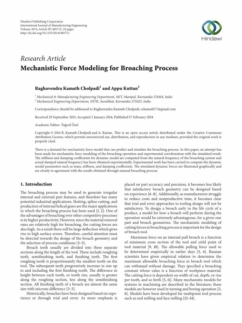
2.3. Results and Discussions. Figures 1(a), 1(b), and 1(c) illus-trate the cutting force versus chip thickness during shapingoperation for the mild steel material. In the plot, 𝑥-axisindicates the logarithm value of chip thickness 𝑡

𝑐and 𝑦-

axis is the logarithm of the cutting forces along 𝑥, 𝑦, and 𝑧

directions, marked as 𝐹𝑥, 𝐹𝑦, and 𝐹

𝑧, respectively in Newton.

The chip thickness is corresponding to depth of cut whichvaried from 0.04mm to 0.16mm. The calibration test isperformed for small depth of cut to avoid the error due toimpulsive cutting forces coming on the workpiece at higherdepth of cut. A linear curve fitting is made using Matlabsoftware to determine the specific energy constants. Toolgeometries were considered the same as the broaching tool.Hence, the variation in specific cutting energy constants is notconsidered for the rake angle variation in the tool.

Negative slope linear curves are obtained and the coef-ficients of the linear curve fitting give the specific cuttingenergy constants. The proportionality constants 𝐾

𝑥, 𝐾𝑦, and

𝐾𝑧are determined using (3). Tables 1 and 2 give the values

of specific cutting energy constants and proportionalityconstants for materials mild steel, aluminium, and cast iron,respectively.

3. Static Model

Accurate modeling of cutting force is required to predictthe vibration, surface quality, and stability of the machiningprocess [20]. In the static force model, axial cutting force,𝐹𝑥during broaching is acting on the tooth as the product

International Journal of Manufacturing Engineering 3

8

8.1

8.2

8.3

8.4

8.5

8.6

8.7

8.8

8.9

9

−3.2 −3 −2.8 −2.6 −2.4 −2.2 −2 −1.8

log(tc)

log(Fx

)

Work: mild steel

y = −0.46 ∗ x + 7.3

(a) Graph for determining a0and a1

7

7.1

7.2

7.3

7.4

7.5

7.6

7.7

7.8

−3.4 −3.2 −3 −2.8 −2.6 −2.4 −2.2 −2 −1.8

log(tc)

log(Fy

)

y =

Work: mild steel−0.037 ∗ x + 7.2

(b) Graph for determining b0and b1

4.8

5

5.2

5.4

5.6

5.8

6

6.2

6.4

−3.2 −3 −2.8 −2.6 −2.4 −2.2 −2 −1.8

log(tc)

log(Fz

)

Work: mild steel

y = −0.71 ∗ x + 3.6

(c) Graph for determining c0and c1

Figure 1: Specific cutting energy constants for mild steel obtainedduring shaping operation.

Table 1: Specific cutting energy constants during shaping process.

Material 𝑎0

𝑎1

𝑏0

𝑏1

𝑐0

𝑐1

Mild steel 7.3 −0.46 7.2 −0.037 3.6 −0.71Aluminium 7.4 −0.39 5.0 −0.68 2.1 −1.2Cast iron 7.3 −0.29 5.9 −0.31 2.3 −1.0

Table 2: Proportionality constants for broaching process.

Material 𝐾𝑥(N/mm2) 𝐾

𝑦(N/mm2) 𝐾

𝑧(N/mm2)

Mild steel 5732.3 1654.0 307.1Aluminium 5370.0 1088.0 279.4Cast iron 3562.0 924.4 199.5

of chip cross section area 𝐴𝑐and a proportionality constant,

𝐾𝑥. Similarly normal force 𝐹

𝑦acting along the cutting

edge is obtained by multiplying the chip cross section areawith proportionality constant 𝐾

𝑦and lateral force 𝐹

𝑧is

similarly obtained by multiplying chip cross section area byproportionality constant, 𝐾

𝑧. The values of 𝐾

𝑥, 𝐾𝑦, and 𝐾

𝑧

are determined by simple calibration test using the shapingoperation.

A static analysis calculates the effects of steady loadingconditions on a structure, while ignoring inertia and dampingeffects, such as those caused by time-varying loads. A staticanalysis can, however, include steady inertia loads (such asgravity and rotational velocity) and time-varying loads thatcan be approximated as static equivalent loads [21, 22].

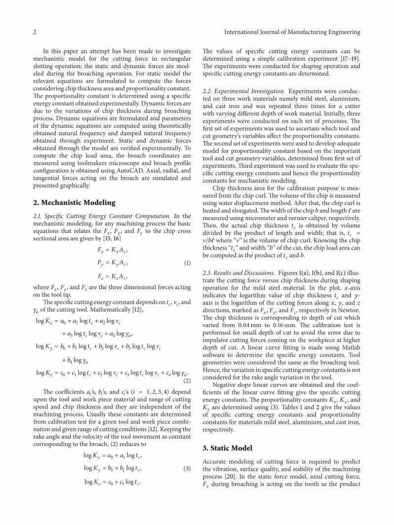
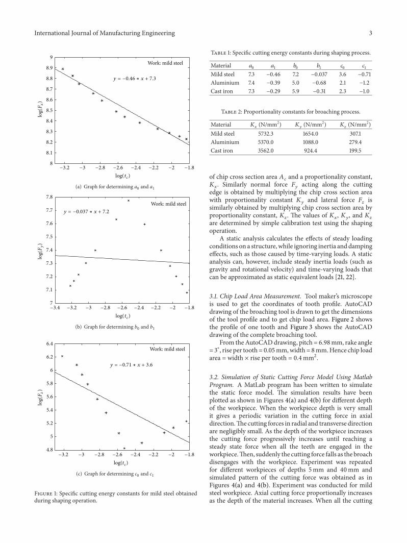
3.1. Chip Load Area Measurement. Tool maker’s microscopeis used to get the coordinates of tooth profile. AutoCADdrawing of the broaching tool is drawn to get the dimensionsof the tool profile and to get chip load area. Figure 2 showsthe profile of one tooth and Figure 3 shows the AutoCADdrawing of the complete broaching tool.

From theAutoCADdrawing, pitch = 6.98mm, rake angle= 3∘, rise per tooth = 0.05mm,width= 8mm.Hence chip loadarea = width × rise per tooth = 0.4mm2.

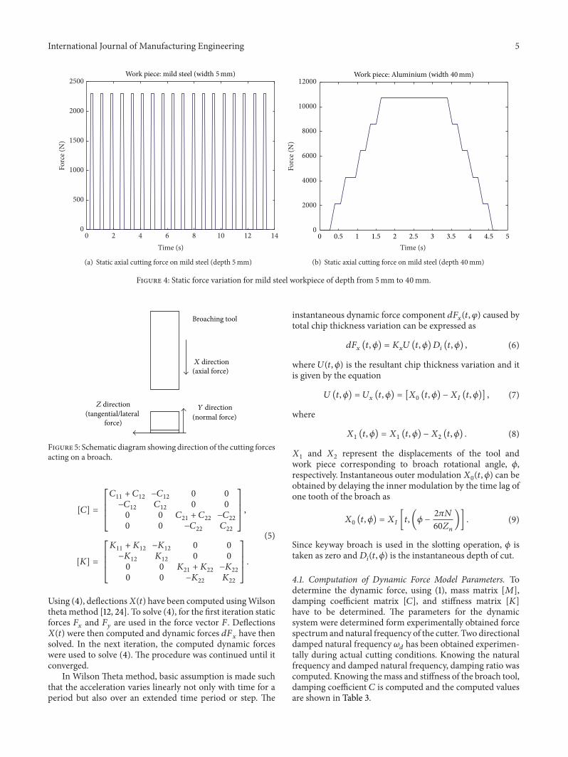
3.2. Simulation of Static Cutting Force Model Using MatlabProgram. A MatLab program has been written to simulatethe static force model. The simulation results have beenplotted as shown in Figures 4(a) and 4(b) for different depthof the workpiece. When the workpiece depth is very smallit gives a periodic variation in the cutting force in axialdirection.The cutting forces in radial and transverse directionare negligibly small. As the depth of the workpiece increasesthe cutting force progressively increases until reaching asteady state force when all the teeth are engaged in theworkpiece.Then, suddenly the cutting force falls as the broachdisengages with the workpiece. Experiment was repeatedfor different workpieces of depths 5mm and 40mm andsimulated pattern of the cutting force was obtained as inFigures 4(a) and 4(b). Experiment was conducted for mildsteel workpiece. Axial cutting force proportionally increasesas the depth of the material increases. When all the cutting


(3.26, 5.20)

(4.97, 6.52)

(6.78, 8.52)(8.02, 8.56)

(7.52, 6.00)

Figure 2: Broach tooth profile obtained from Toolmaker’s micro-scope and AutoCAD drawing.

1.27

1.23

1.18

1.13

1.09

1.04

0.99

0.94

0.9

0.85

0.8

0.76

0.71

0.66

0.61

0.57

0.52

0.47

0.43

0.38

0.33

0.28

0.24

0.19

0.14

0.1

0.05

6.98

Figure 3: AutoCAD drawing of broach tool.

tips are engaged in the workpiece the cutting force requiredis stable at a steady state cutting conditions.

For higher depth of the workpiece, initial increase inthe cutting forces, there is a step by step increase in thecutting forces. This clearly indicates the engagement of thecutting tooth as the broach goes inside the workpiece. Whenthe depth of the workpiece is less than 5mm, the nature ofthe cutting force is periodic and frequency of the spectrumobtained from the graph shows maximum cutting force at40Hz. This indicates that cutting force variation mainlydepends upon the chip thickness variation since there is nopeak values observed at higher frequency.The feed rate of thebroach is 10mm/second.

4. Development of Dynamic Force Model

The broaching operation uses only two dimensional modelsand cutting force in lateral direction is negligibly small andnot relevant. This is because axial force is more predominantand lateral force is very small in comparison. Figure 5 showsthe cutting force direction on a broaching tool.

Broaching is analyzed as orthogonal cutting because thechip velocity is orthogonal to the cutting edge in the slottingoperation. Even though all the cutting processes are obliquecutting, in the case of broaching, the cutting happens to bein depth-wise, hence, the assumption of orthogonal cuttingis valid [23–25].

For determining the dynamic cutting forces, the twodegrees of freedom vibratory system is considered and themodel parameters of the machine tool structural system havebeen determined. By assuming that worktable and spindlehead of the machine tool are rigid bodies, the vibratorysystem of the workpiece and tool in a one directionalreference system was modeled as two degrees of freedomsystem as shown in Figure 6. The parameters of this systemwere determined from the theoretical natural frequenciesand damped natural frequency corresponding to frequencyobtained from the actual cutting system.

Assuming tool and workpiece as a rigid body, the systemcan be modeled as

[𝑀] �� + [𝐶] �� + [𝐾]𝑋 = [𝐹] , (4)

where 𝑋 = {𝑥1

𝑥2

𝑦1

𝑦2}𝑇 is the relative displacement

vector between tool and workpiece and 𝐹 = {𝐹𝑥

0 𝐹𝑦

0}𝑇

is the force vector; [𝑀] is the mass matrix which dependson tool and workpiece and [𝐶] is the damping coefficientwhich depends on cutting feed and speed between the tooland workpiece and [𝐾] is the stiffness matrix connecting thetool and workpiece.

The values for [𝑀], [𝐶], and [𝐾] are:

[𝑀] =

[[[

[

𝑀1

0 0 0

0 𝑀2

0 0

0 0 𝑀1

0

0 0 0 𝑀2

]]]

]

,


0 2 4 6 8 10 12 140

500

1000

1500

2000

2500

Time (s)

Forc

e (N

)Work piece: mild steel (width 5mm)

(a) Static axial cutting force on mild steel (depth 5mm)

0

2000

4000

6000

8000

10000

12000

Time (s) 0 0.5 1 1.5 2 2.5 3 3.5 4 4.5 5

Forc

e (N

)

Work piece: Aluminium (width 40mm)

(b) Static axial cutting force on mild steel (depth 40mm)

Figure 4: Static force variation for mild steel workpiece of depth from 5mm to 40mm.

X direction(axial force)

Broaching tool

Y direction(normal force)

Z direction(tangential/lateral

force)

Figure 5: Schematic diagram showing direction of the cutting forcesacting on a broach.

[𝐶] =

[[[

[

𝐶11

+ 𝐶12

−𝐶12

0 0

−𝐶12

𝐶12

0 0

0 0 𝐶21

+ 𝐶22

−𝐶22

0 0 −𝐶22

𝐶22

]]]

]

,

[𝐾] =

[[[

[

𝐾11

+ 𝐾12

−𝐾12

0 0

−𝐾12

𝐾12

0 0

0 0 𝐾21

+ 𝐾22

−𝐾22

0 0 −𝐾22

𝐾22

]]]

]

.

(5)

Using (4), deflections𝑋(𝑡) have been computed usingWilsontheta method [12, 24]. To solve (4), for the first iteration staticforces 𝐹

𝑥and 𝐹

𝑦are used in the force vector 𝐹. Deflections

𝑋(𝑡) were then computed and dynamic forces 𝑑𝐹𝑥have then

solved. In the next iteration, the computed dynamic forceswere used to solve (4). The procedure was continued until itconverged.

In Wilson Theta method, basic assumption is made suchthat the acceleration varies linearly not only with time for aperiod but also over an extended time period or step. The

instantaneous dynamic force component 𝑑𝐹𝑥(𝑡, 𝜑) caused by

total chip thickness variation can be expressed as

𝑑𝐹𝑥(𝑡, 𝜙) = 𝐾

𝑥𝑈 (𝑡, 𝜙)𝐷

𝑖(𝑡, 𝜙) , (6)

where 𝑈(𝑡, 𝜙) is the resultant chip thickness variation and itis given by the equation

𝑈(𝑡, 𝜙) = 𝑈𝑥(𝑡, 𝜙) = [𝑋

0(𝑡, 𝜙) − 𝑋

𝐼(𝑡, 𝜙)] , (7)

where

𝑋1(𝑡, 𝜙) = 𝑋

1(𝑡, 𝜙) − 𝑋

2(𝑡, 𝜙) . (8)

𝑋1and 𝑋

2represent the displacements of the tool and

work piece corresponding to broach rotational angle, 𝜙,respectively. Instantaneous outer modulation 𝑋

0(𝑡, 𝜙) can be

obtained by delaying the inner modulation by the time lag ofone tooth of the broach as

𝑋0(𝑡, 𝜙) = 𝑋

𝐼[𝑡, (𝜙 −

2𝜋𝑁

60𝑍𝑛

)] . (9)

Since keyway broach is used in the slotting operation, 𝜙 istaken as zero and 𝐷

𝑖(𝑡, 𝜙) is the instantaneous depth of cut.

4.1. Computation of Dynamic Force Model Parameters. Todetermine the dynamic force, using (1), mass matrix [𝑀],damping coefficient matrix [𝐶], and stiffness matrix [𝐾]

have to be determined. The parameters for the dynamicsystem were determined form experimentally obtained forcespectrum and natural frequency of the cutter. Two directionaldamped natural frequency 𝜔

𝑑has been obtained experimen-

tally during actual cutting conditions. Knowing the naturalfrequency and damped natural frequency, damping ratio wascomputed. Knowing themass and stiffness of the broach tool,damping coefficient 𝐶 is computed and the computed valuesare shown in Table 3.


Work

Machine tool

Broach lob

Broach tool tip

X1

X2

C11C12

C22

C21

K22

K12K11

K21

M2

M2M1

Ff

Fn

h0 + dy

h0

Figure 6: Dynamic force model for broaching.

Table 3: Damping coefficients and stiffness parameters for dynamicmodel.

Damping coefficients Value(N/mm/sec) Stiffness parameters Value

(N/mm)𝑐11

𝑐21

140 𝑘11

𝑘12

7.0 × 106

𝑐12

𝑐22

60 𝑘21

𝑘22

6.0 × 106

Figure 7: Photograph of a Push type broaching machine.

The computed mass, stiffness, and damping coefficientmatrix are

[𝑀] =

[[[

[

0.35 0 0 0

0 0.116 0 0

0 0 0.35 0

0 0 0 0.116

]]]

]

,

[𝐾] = 106[[[

[

23 −9 0 0

−9 23 0 0

0 0 17 −6

0 0 −6 15

]]]

]

,

Accelerometer

Broaching tool

Main spindle

Figure 8: Photograph indicating the position of an accelerometer.

[𝐶] =

[[[

[

200 −60 0 0

−60 150 0 0

0 0 200 −50

0 0 −50 50

]]]

]

. (10)

5. Experimental Setup

The experimental setup includes a push type broachingmachine as shown in Figure 7 which was used for measuringthe cutting force in three directions, keyway broach, Kistleraccelerometer, and data acquisition system.The data acquisi-tion system consists of hardware unit and an application pro-gramming interface. The real-time analog signals obtainedfrom the accelerometer are sent to the hardware unit. Thehardware unit performs the conditioning like amplificationand filtering of the signals to increase the signal-to-noiseratio. This conditioned analog signal is sent through theproper cables to a data acquisition card which has electronicintegrated circuit to convert the analog signal into the digitalcounterpart and sends the signal to the computer for furtherprocessing where it can store 1000 characters per second datain the computer.The program in the personal computer (PC)written using the Application Programming Interface (API)software performs the relevant operations on the input signal


0 5 10 15 20 25 300

500

1000

1500

2000

2500

3000

3500

4000

NormalThrust

Tangential

Work: M.S.Width: 10mm

Length (mm)

Forc

e (N

)

(a) Cutting forces for 10mm depth

0 20 40 60 80 100 1200

2000

4000

6000

8000

10000

12000 Width: 40mm

NormalThrust

Tangential

Work: M.S.

Length (mm)

Forc

e (N

)(b) Cutting forces for 40mm depth

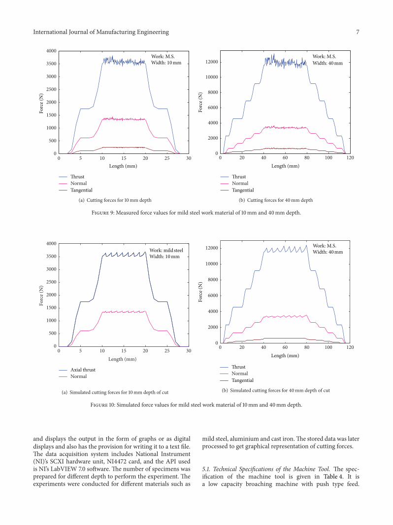
Figure 9: Measured force values for mild steel work material of 10mm and 40mm depth.

0 5 10 15 20 25 300

500

1000

1500

2000

2500

3000

3500

4000

Length (mm)

Forc

e (N

)

Work: mild steelWidth: 10mm

NormalAxial thrust

(a) Simulated cutting forces for 10mm depth of cut

0 20 40 60 80 100 1200

2000

4000

6000

8000

10000

12000Width: 40mm

NormalThrust

Tangential

Work: M.S.

Length (mm)

Forc

e (N

)

(b) Simulated cutting forces for 40mm depth of cut

Figure 10: Simulated force values for mild steel work material of 10mm and 40mm depth.

and displays the output in the form of graphs or as digitaldisplays and also has the provision for writing it to a text file.The data acquisition system includes National Instrument(NI)’s SCXI hardware unit, NI4472 card, and the API usedis NI’s LabVIEW 7.0 software. The number of specimens wasprepared for different depth to perform the experiment. Theexperiments were conducted for different materials such as

mild steel, aluminium and cast iron.The stored data was laterprocessed to get graphical representation of cutting forces.

5.1. Technical Specifications of the Machine Tool. The spec-ification of the machine tool is given in Table 4. It isa low capacity broaching machine with push type feed.


0 20 40 60 80 100 1200

2000

4000

6000

8000

10000

12000Width: 40mmWork: M.S.

Length (mm)

Thru

st fo

rce (

N)

(a) Cutting forces in axial direction

0 20 40 60 80 100 1200

500

1000

1500

2000

2500

3000

3500Width: 40mmWork: M.S.

Length (mm)

Nor

mal

forc

e (N

)

(b) Cutting forces in normal direction

0 20 40 60 80 100 1200

100

200

300

400

500

600

700

Tang

entia

l for

ce (N

)

Length (mm)

Work: M.S.Width: 40mm

SimulatedMeasured

(c) Cutting forces in lateral direction

Figure 11: Comparison of measured and simulated force valuesduring broaching operation on mild steel work.

Table 4: Technical specifications.

Maximum push load capacity 5000 kgMaximum stroke 500mmFace plate dimension 405 × 210mmSlot dimension in face plate 100mmBroaching speed 1.5m/minReturn speed 3m/minPower of electric motor 1.5 kW/2HP/1500 RPM

Thephotograph of the accelerometer position on themachinetool is shown in Figure 8.

6. Results and Discussions

Figures 9(a) and 9(b) show the measured values of cuttingforces acting on mild steel workpiece of 10mm and 40mmdepth, respectively. The pattern of experimental result isclosely in agreement with mechanistic model results inFigures 10(a) and 10(b). The percentage of error betweenexperimental results and mechanistic model results is within2%.

Figures 11(a), 11(b), and 11(c) show the comparison ofexperimental results with simulated results for cutting forcevariation for a mild steel workpiece of 40mm depth inaxial, normal, and lateral directions. As height of the workpiece increases, forces are also increasing and repeatedly insinusoidal manner and come to zero as broach disengageswith the work piece.

The experiment and simulated results shown in Figures11(a), 11(b), and 11(c) confirm that axial force is very muchhigher than normal force for both 40mmand 10mmdepth ofmild steel workmaterial.The force in the tangential directionis even smaller in comparison to the axial force.

7. Conclusions

This paper reports the dynamic force modeling of broachingprocess and validation of output with experimental results.A software has been developed to compute the dynamicforces using Matlab. Experiment has been carried out usinga vertical broaching machine for the mild steel materialof different depths. Experimental validations of the cuttingforces are required to establish the prediction from themodelso that themodel is acceptable to themanufacturing industry.Thework piece is themost complicated link of themachiningsystem. The second validation deals with a case where amachine tool spindle is the weakest part of the system. Thefixture of the work piece for the broaching was mountedsuch that feed direction becomes very compliant. Slots wereprovided on the fixture so that cutter can perform axissymmetry cutting. The position of the cutter also permits aproper pressing action on the fixture so that cutting processhas effect on the overall stability of the cutting process.

The parameters which affect the cutting process aredepth of cut, feed rate and cutter geometry. The feed rate,determines the axial chip load. Overall stability increases


as the feed rate is increased. This is due to the fact thatspecific cutting energy constant decreases as a function ofchip load. Stability in general is accountable for dynamicsin the axial direction for broaching because the work pieceand machine tool dynamics in axial direction are usually oforder of magnitude stiffer than in the normal direction. Theoccurrence of the chatter predominant during the experi-ment is largely dependent on the material specific cuttingenergy constants since they determine the magnitude of theforces which present during machining. During broaching,the work holding fixture has an important role to play incontrolling the force acting on the tool. Major force actingon the broaching tool is in axial direction.

All the factors discussed above that affect stability anddynamics of the structural system are influential. A goodunderstanding of how the dynamics affect the overall stabilitycan be helpful to assess the quality of the product.Thedynam-ics variables include stiffness, damping, natural frequency,and mode cycles. Special care has to be taken to ensure thatexperimentally collected data is clear and accountable. Thesimulated and experimental results are presented graphicallyand are in close agreement. It is concluded that mechanisticmodel is suitable for determining cutting forces for broachingprocess.

Nomenclature

𝐴𝑐: Chip cross-section area

𝑎𝑖, 𝑏𝑖, 𝑐𝑖: Specific cutting energy constants

𝐹𝑎: Axial cutting force

𝐹𝑡: Tangential cutting force

𝐹𝑛: Normal cutting force

𝐾𝑥, 𝐾𝑦, 𝐾𝑧: Proportionality constants

𝑡𝑐: Chip thickness

V𝑐: Cutting velocity

𝛾𝑎: Rake angle.

Conflict of Interests

The authors declare that there is no conflict of interestsregarding the publication of this paper.

Acknowledgments

The authors would like to express their gratitude and sincerethanks to Professor Dr. Appu Kuttan, Director, MANIT,Bhopal (MP), for guidance, valuable help, enthusiastic atti-tude, and suggestions throughout the period and NationalInstitute of Technology Karnataka (NITK) Surathkal, forproviding necessary facilities to conduct experiments.

References

[1] E. Linsley Horace, Broaching Tooling and Practice, IndustrialPress, 1961.

[2] C. Monday, Broaching, Machinery Publication, London, UK,1960.

[3] J. W. Sutherland, E. J. Salisbury, and F. W. Hoge, “A modelfor the cutting force system in the gear broaching process,”

International Journal of Machine Tools andManufacture, vol. 37,no. 10, pp. 1409–1421, 1997.

[4] V. S. Belov and S. M. Ivanov, “Factors affecting broachingcondition and broach life,” Journal of Stanki Instruments, vol.45, pp. 31–33, 1974.

[5] E. Kuljanic, “Cutting force and surface roughness in broaching,”Annual CIRP, vol. 24, no. 1, pp. 77–82, 1975.

[6] M. E. Merchant, “Mechanics of the metal cutting process. I.Orthogonal cutting and a type 2 chip,” Journal of Applied Physics,vol. 16, no. 5, pp. 267–275, 1945.

[7] M. E. . Merchant, “Basic mechanics of the metal cuttingprocess,” Journal of Applied Mechanics, vol. 168, pp. 175–178,1954.

[8] T. Tyan and W. H. Yang, “Analysis of orthogonal metal cuttingprocesses,” International Journal for Numerical Methods inEngineering, vol. 34, no. 1, pp. 365–389, 1992.

[9] V. Sajeev, L. Vijayraghavan, and U. R. K. Rao, “An analysis of theeffect of burnishing in internal broaching,” International Journalof Mechanical Engineering, vol. 28, pp. 163–173, 2000.

[10] D. A. Axinte and N. Gindy, “Tool condition monitoring inbroaching,” Journal ofWear, vol. 254, no. 3-4, pp. 370–382, 2003.

[11] B. Daniel Dallas, Tool and Manufacturing Engineers Handbook,3rd edition, 2002.

[12] H. S. Kim and K. F. Ehmann, “A cutting force model for facemilling operations,” International Journal of Machine Tools andManufacture, vol. 33, no. 5, pp. 651–673, 1993.

[13] H. J. Fu, R. E. DeVor, and S. G. Kapoor, “A mechanistic modelfor the prediction of the force system in facemilling operations,”Journal of Engineering for Industry, Transactions of the ASME,vol. 106, no. 1, pp. 81–88, 1984.

[14] E. Felder, P. Gillormini, L. Tronchet, and F. Leroy, “A compara-tive analysis of threemachining process: broaching, tapping andslotting,” etude DGRST Materiaux, vol. 80, pp. 512–513, 1982.

[15] S. G. Kapoor, R. E. DeVor, R. Zhu, R. Gajjela, G. Parakkal,and D. Smithey, “Development of mechanistic models forthe prediction of machining performance: model buildingmethodology,” Machining Science and Technology, vol. 2, no. 2,pp. 213–238, 1998.

[16] S. Jayaram, S. G. Kapoor, and R. E. Devor, “Estimation of thespecific cutting pressures for mechanistic cutting force models,”International Journal of Machine Tools andManufacture, vol. 41,no. 2, pp. 265–281, 2001.

[17] E. Usui, A. Hirota, and M. Masuko, “Analytical predictionsof three dimensional cutting process—part I: basic cuttingmodel an energy approach,” Journal of Engineering for Industry,Transactions of the ASME, vol. 100, no. 2, pp. 222–228, 1978.

[18] W. J. Endres, R. E. DeVor, and S. G. Kapoor, “A dual mechanismapproach to the prediction of machining forces,” ASME Journalof Engineering For Industry, vol. 117, no. 4, pp. 526–533, 1999.

[19] J. A. Kir, D. K. Anand, and C.Mahindra, “Matrix representationand prediction of three dimensional cutting forces,” ASMEJournal of Engineering For Industry, vol. 99, pp. 822–828, 1978.

[20] F. Koenigsberger and J. Tlusty, Machine Tool Structures-Vol. 1:Stability against Chatter, Pergamon Press, 1967.

[21] P. Albrecht, “Dynamics of the metal cutting process,” ASMEJournal of Engineering for Industry, vol. 87, pp. 429–441, 1965.

[22] J. D. Smith and S. A. Tobias, “The dynamic cutting of metals,”International Journal of Machine Tool Design and Research, vol.1, no. 4, pp. 283–292, 1961.


[23] D. A. Stephenson and S. M. Wu, “Computer models for themechanics of three dimensional cutting process part 1: theoryand numerical methods,” ASME Journal of Engineering forIndustry, vol. 110, no. 1, pp. 32–37, 1988.

[24] H. Q. Zheng, X. P. Li, Y. S. Wong, and A. Y. C. Nee, “Theoreticalmodelling and simulation of cutting forces in face millingwith cutter runout,” International Journal of Machine Tools andManufacture, vol. 39, no. 12, pp. 2003–2018, 1999.

[25] J. A. Yang, V. Jaganathan, and R. Du, “A new dynamic modelfor drilling and reaming processes,” International Journal ofMachine Tools andManufacture, vol. 42, no. 2, pp. 299–311, 2002.

International Journal of

AerospaceEngineeringHindawi Publishing Corporationhttp://www.hindawi.com Volume 2014

RoboticsJournal of

Hindawi Publishing Corporationhttp://www.hindawi.com Volume 2014


Active and Passive Electronic Components

Control Scienceand Engineering

Journal of



RotatingMachinery


Hindawi Publishing Corporation http://www.hindawi.com

Journal ofEngineeringVolume 2014

Submit your manuscripts athttp://www.hindawi.com

VLSI Design



Shock and Vibration


Civil EngineeringAdvances in

Acoustics and VibrationAdvances in



Electrical and Computer Engineering

Journal of

Advances inOptoElectronics

Hindawi Publishing Corporation http://www.hindawi.com

Volume 2014

The Scientific World JournalHindawi Publishing Corporation http://www.hindawi.com Volume 2014

SensorsJournal of


Modelling & Simulation in EngineeringHindawi Publishing Corporation http://www.hindawi.com Volume 2014


Chemical EngineeringInternational Journal of Antennas and

Propagation




Navigation and Observation



DistributedSensor Networks


research article mechanistic force modeling for...

Documents