simbiology for pharmacokinetic and mechanistic modeling · simbiology ® for pharmacokinetic and...

SimBiology®

for Pharmacokinetic and Mechanistic Modeling

CHAPTER 1 COURSE LAYOUT .......................................................................................................... 1

CHAPTER 2 NAVIGATING THE SIMBIOLOGY DESKTOP.................................................................... 2

Topics Covered .................................................................................................................................. 2

Starting SimBiology ........................................................................................................................... 2

SimBiology Desktop ........................................................................................................................... 2

SimBiology Project ............................................................................................................................ 3

Working with a SimBiology Project ................................................................................................... 5

Adding Model, Task or Dataset to the Project .................................................................................. 7

Exercise.............................................................................................................................................. 7

CHAPTER 3 DATA IMPORT .............................................................................................................. 8

Topics Covered .................................................................................................................................. 8

Importing Data from Files ................................................................................................................. 9

Working with Imported Data .......................................................................................................... 12

Plotting and Visualizing Imported Data........................................................................................... 13

Excluding Data Rows ....................................................................................................................... 16

Creating Additional Data Columns .................................................................................................. 18

Exercise............................................................................................................................................ 19

CHAPTER 4 PARAMETER ESTIMATION .......................................................................................... 21

Topics Covered ................................................................................................................................ 21

Parameter Estimation in SimBiology ............................................................................................... 21

Adding a Parameter Estimation Task .............................................................................................. 22

Configuring the Fit Parameters Task: Individual Fitting .................................................................. 23

Individual Fitting: Results and Diagnostic Plots .............................................................................. 27

Exercise............................................................................................................................................ 30

CHAPTER 5 MODELING: CREATING PK MODELS ........................................................................... 32

Topics Covered ................................................................................................................................ 32

The MODEL Tab ............................................................................................................................... 32

Creating Pharmacokinetic Models .................................................................................................. 34

CHAPTER 6 MODELING: CREATING CUSTOM MODELS ................................................................ 37

Topics Covered ................................................................................................................................ 37

Understanding the building blocks: ................................................................................................ 37

Working in the Diagram View ......................................................................................................... 38

Creating a Custom Model ................................................................................................................ 40

Adding Blocks .................................................................................................................................. 41

Connecting Blocks ........................................................................................................................... 43

Compartment Properties ................................................................................................................ 44

Species Properties ........................................................................................................................... 45

Defining Reaction Properties .......................................................................................................... 46

Defining Parameter Properties ....................................................................................................... 47

Reaction Rate Expressions .............................................................................................................. 47

Interpretation of Variables in Reaction Rate Expressions ............................................................... 50

Block Appearance and Description Properties................................................................................ 50

Working with the Table View .......................................................................................................... 52

Introduction to Rules ...................................................................................................................... 53

Adding Rules .................................................................................................................................... 54

Rule properties ................................................................................................................................ 54

Rule Expression ............................................................................................................................... 55

Exercise............................................................................................................................................ 57

CHAPTER 7 SIMULATING AND ANALYZING MODELS .................................................................... 60

Topics Covered ................................................................................................................................ 60

Adding a Task .................................................................................................................................. 61

Running a Task ................................................................................................................................ 61

The TASK Tab ................................................................................................................................... 62

Modifiers: Doses & Variants ............................................................................................................ 63

Adding Doses ................................................................................................................................... 63

Adding Variants ............................................................................................................................... 66

Using Modifiers in tasks .................................................................................................................. 66

Dimensional Analysis ....................................................................................................................... 68

Unit Conversion ............................................................................................................................... 69

Chapter 1 Course Layout

1

Chapter 1 Course Layout

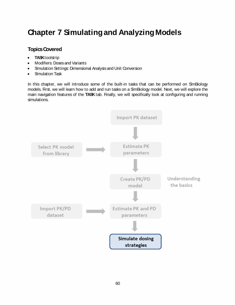
In this course, we will teach major concepts in SimBiology using simple examples of pharmacokinetic (PK) and simultaneous pharmacokinetic/pharmacodynamic (PK/PD) analyses. The example will begin with importing a PK dataset from a single subject, single oral dose study. After some basic preprocessing and visualization, we will fit the data to a one compartmental PK model with first-order dosing and linear elimination.

Next, we will combine the PK model with an indirect response PD model. We will fit a combined PK/PD dataset to this model and simultaneously estimate the PK and the PD parameters. Finally, we will use the PK/PD estimates to simulate the drug and efficacy profiles for single and repeated dose regimen.

The layout of the course is illustrated below.

Chapter 2 Navigating the SimBiology Desktop

2


Topics Covered

SimBiology desktop overview

SimBiology project

Toolstrip and the HOME tab

Starting SimBiology

Open the SimBiology desktop by typing simbiology in the MATLAB Command Window.

Try >>

Open SimBiology desktop

SimBiology Desktop

The SimBiology desktop is a graphical user interface, made up of a set of integrated tools, designed to build, simulate, and analyze dynamic models. The SimBiology desktop has three primary components:

Toolstrip – Displays the HOME tab and other contextual tabs depending on selected project component

Address Bar — Displays the path breadcrumbs to the selected project component and can be used to navigate between components

Work Area – Displays the contents of the selected project component

You can plug in additional tools (Block Library Browser, MATLAB Code Capture Tool, etc.) in the

SimBiology desktop by selecting from the Tools list on the HOME tab. Desktop tools can be

minimized, maximized, docked, restored and closed using the options under the Action button in the tool window.


3

Tip To reset the desktop to the default layout, select View > Desktop Layout > Default Layout in the HOME tab

SimBiology Project

Work done in the SimBiology desktop can be saved as a SimBiology project file. A SimBiology project is comprised of models, datasets and tasks. The file extension for a SimBiology project file is .sbproj.


4

To save your work, click on Save in the HOME tab or use Ctrl + S. If you are saving your work for the first time, the Save SimBiology Project dialog box opens. Specify the location and name of the project, and click Save.

Tip Remember to periodically save the project by selecting Save in the HOME tab or with Ctrl + S

To open an existing project, click on Open in the HOME tab or use Ctrl + Shift + O. The Open SimBiology Project dialog opens. Navigate to the file location, select the .sbproj file to be opened and click Open.

You can use the New or Close options in the HOME tab to create a new SimBiology project or close the current project in the desktop.

Tip You can quickly open recent project files from the Quick Start page. The quick start page can be accessed by Home > Quick Start in the Address Bar OR by clicking on the Quick Start icon in the toolstrip.

Try >> Open Sample_Project.sbproj in the SimBiology Training folder


5

Working with a SimBiology Project

The Project page displays a list of models, tasks and data in the current project. You have 2 options to get to the Project page:

Click on the View Contents button in the HOME tab, OR In the Address Bar, go to Home > Project

Similarly, the Models, Tasks and Data pages display a list of models, tasks and datasets, respectively. These pages exists one level below the Project page.


6

To open or modify a model, data or task:

Double-click on the component on the Project (or Models, Tasks and Data) page. [The Address Bar will update to show the path breadcrumbs of the opened component. Additional contextual tabs may appear in the toolstrip. In some cases, toolstrip tab might change to the contextual tab]

Tip You can use the path breadcrumbs on the Address Bar to directly navigate to a project component


7

Adding Model, Task or Dataset to the Project

To add a model, task or data to the current project:

Select the Add Model, Add Task, or Add Data options in the HOME tab.

You can also add components (model, tasks and datasets) to the project from the MODEL and TASK tabs. We will look at this in later chapters.

Tip The number next to the Add Model, Add Task and Add Data button on the HOME tab indicates the number of models, tasks and datasets, respectively, in the current project. Click on the number to directly navigate to the Models, Tasks or Data page

Exercise

Navigate to the Project page using View Contents. o Name the models present in the Sample_Project project

Open the PKPD_Data dataset o Name the contextual tabs that open in the toolstrip when a dataset is opened. Go to the Explore

Data tab Using the Address Bar, navigate to the Models page

o Open the Two Comp PK model o Open MODEL tab

8

Chapter 3 Data Import

Topics Covered

Data sources

Working with imported data

Visualization

Excluding data

Creating derived data

In this chapter, we will import a PK dataset from a Microsoft Excel® file, and perform some basic visualization and preprocessing on the imported data.

9

Importing Data from Files

Data can be imported into the SimBiology desktop from the following sources:

Tabular text file

Microsoft Excel

file

Variables (dataset object, time series objects, or a SimData object) from the MATLAB workspace or MAT files

Data from SimBiology projects (.sbproj file)

To import data from an Excel file:

Click Add Data in the HOME tab and select the Load Data from File option. [The import data from file dialog opens.] Select the Excel file to be imported, and click Open. [The Excel File Import dialog opens, and displays a preview of the data (first 20 rows).]

If the first row contains header information, check the First Row Contains Header Information box.

<Optional> Edit column names. Note that column names cannot be changed once the data is imported into SimBiology

Click OK

11

To import data from a tabular text file:

Select Add Data in the HOME tab. [The import data from file dialog opens.] Select the text file to be opened, and click Open. [The Text File Import dialog opens, and displays a preview of the data (first 20 rows).]

Specify the Column Separator. The Auto-detect option should detect common delimiters. Note that each row and column in the text file must have the same type and number of delimiters.

If the first row contains header information, check the First Row Contains Header Information box.

In the Treat __ as Missing Values box, specify the character used to indicate missing data points. Missing value character must be a non-numeric character. The default missing value character is a period (.). Missing data points will be imported and interpreted as NaN in SimBiology.

<Optional> Edit column names. Note that column names cannot be changed once the data is imported into SimBiology

Click OK

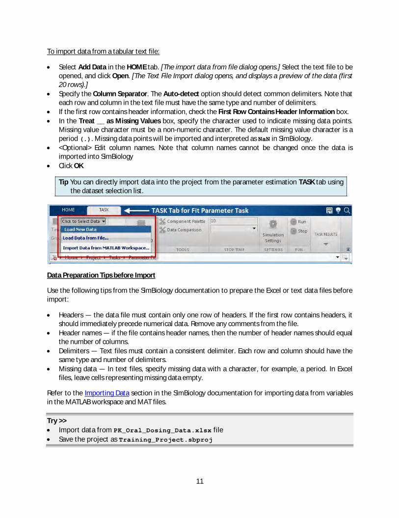
Tip You can directly import data into the project from the parameter estimation TASK tab using the dataset selection list.

Data Preparation Tips before Import

Use the following tips from the SimBiology documentation to prepare the Excel or text data files before import:

Headers — the data file must contain only one row of headers. If the first row contains headers, it should immediately precede numerical data. Remove any comments from the file.

Header names — if the file contains header names, then the number of header names should equal the number of columns.

Delimiters — Text files must contain a consistent delimiter. Each row and column should have the same type and number of delimiters.

Missing data — In text files, specify missing data with a character, for example, a period. In Excel files, leave cells representing missing data empty.

Refer to the Importing Data section in the SimBiology documentation for importing data from variables in the MATLAB workspace and MAT files.

Try >>

Import data from PK_Oral_Dosing_Data.xlsx file

Save the project as Training_Project.sbproj

12

Working with Imported Data

Once the data is imported into SimBiology, you can visualize and pre-process it

To view the imported dataset:

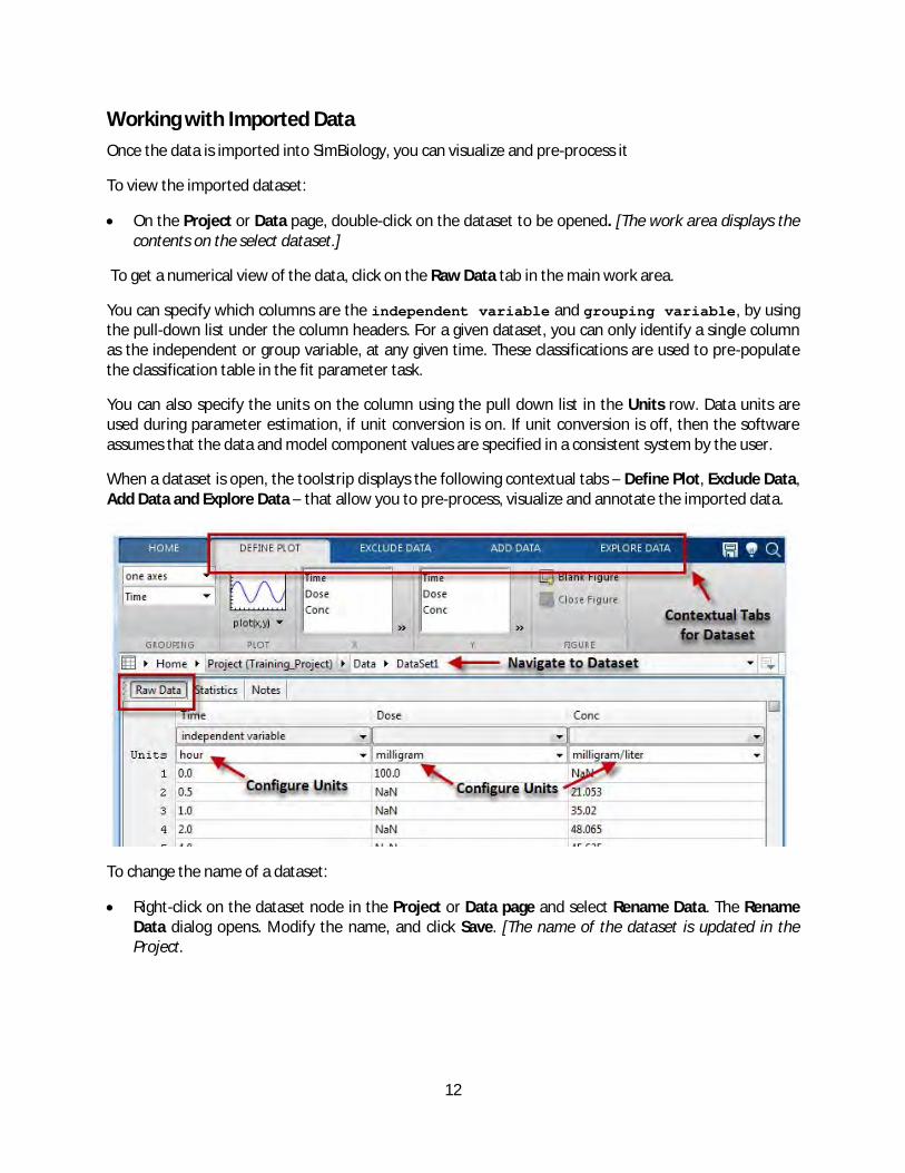
On the Project or Data page, double-click on the dataset to be opened. [The work area displays the contents on the select dataset.]

To get a numerical view of the data, click on the Raw Data tab in the main work area.

You can specify which columns are the independent variable and grouping variable, by using the pull-down list under the column headers. For a given dataset, you can only identify a single column as the independent or group variable, at any given time. These classifications are used to pre-populate the classification table in the fit parameter task.

You can also specify the units on the column using the pull down list in the Units row. Data units are used during parameter estimation, if unit conversion is on. If unit conversion is off, then the software assumes that the data and model component values are specified in a consistent system by the user.

When a dataset is open, the toolstrip displays the following contextual tabs – Define Plot, Exclude Data, Add Data and Explore Data – that allow you to pre-process, visualize and annotate the imported data.

To change the name of a dataset:

Right-click on the dataset node in the Project or Data page and select Rename Data. The Rename Data dialog opens. Modify the name, and click Save. [The name of the dataset is updated in the Project.

13

Alternatively, you can access the Rename Data option under the Action Button in the Address Bar when a dataset is opened.

Try >>

Rename the dataset node to PK_Single_PO_Dose

Set the units on the columns as follows: Time in hour, Dose in milligram and Conc in milligram/liter

Plotting and Visualizing Imported Data

To plot the data:

14

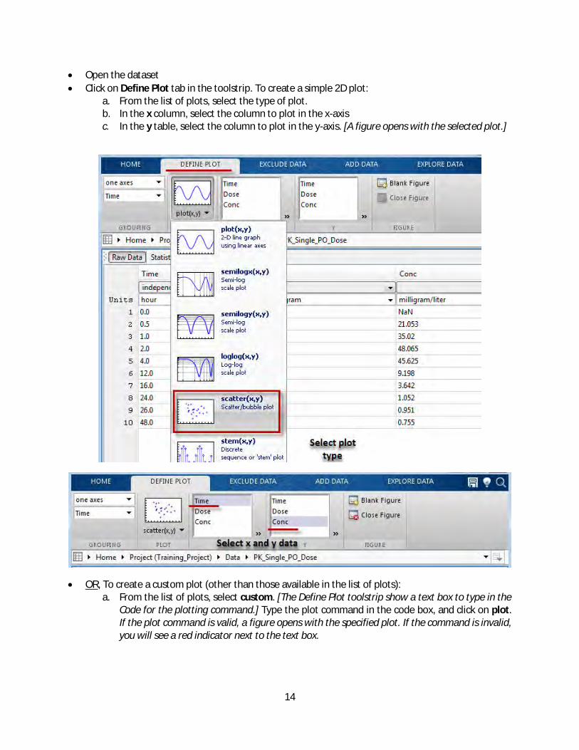
Open the dataset

Click on Define Plot tab in the toolstrip. To create a simple 2D plot: a. From the list of plots, select the type of plot. b. In the x column, select the column to plot in the x-axis c. In the y table, select the column to plot in the y-axis. [A figure opens with the selected plot.]

OR, To create a custom plot (other than those available in the list of plots): a. From the list of plots, select custom. [The Define Plot toolstrip show a text box to type in the

Code for the plotting command.] Type the plot command in the code box, and click on plot. If the plot command is valid, a figure opens with the specified plot. If the command is invalid, you will see a red indicator next to the text box.

15

By default, the new plot will overwrite the existing plot in the data panel. To add the plot in a new figure window, open a new Blank Figure before creating the plot.

Creating grouped lattice plots

To create a grouped lattice plot, change the plot style to separate axes and specify the grouping column in the Define Plot toolstrip

Try >>

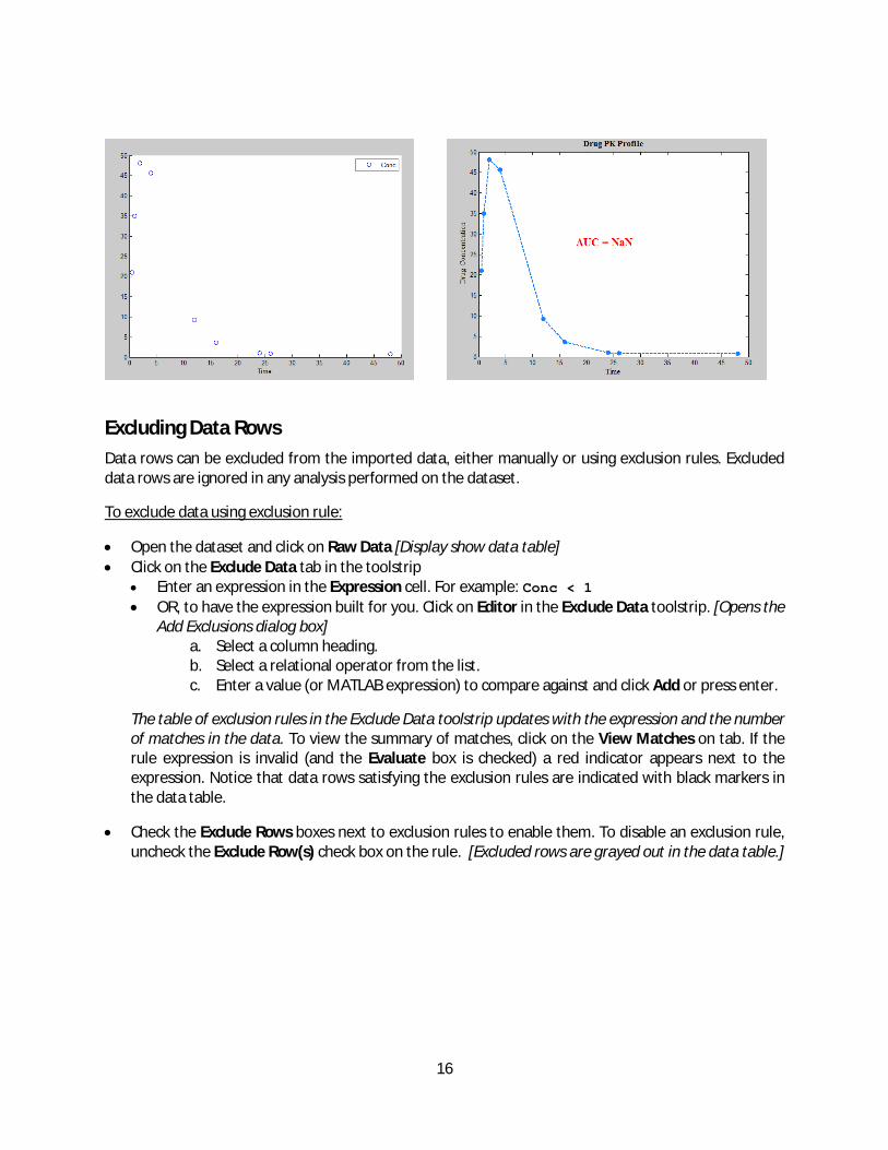
Create a scatter plot of Conc vs. Time

Open a new blank figure. Create the following custom plot: aucPlot(Time, Conc)

16

Excluding Data Rows

Data rows can be excluded from the imported data, either manually or using exclusion rules. Excluded data rows are ignored in any analysis performed on the dataset.

To exclude data using exclusion rule:

Open the dataset and click on Raw Data [Display show data table]

Click on the Exclude Data tab in the toolstrip Enter an expression in the Expression cell. For example: Conc < 1

OR, to have the expression built for you. Click on Editor in the Exclude Data toolstrip. [Opens the Add Exclusions dialog box]

a. Select a column heading. b. Select a relational operator from the list. c. Enter a value (or MATLAB expression) to compare against and click Add or press enter.

The table of exclusion rules in the Exclude Data toolstrip updates with the expression and the number of matches in the data. To view the summary of matches, click on the View Matches on tab. If the rule expression is invalid (and the Evaluate box is checked) a red indicator appears next to the expression. Notice that data rows satisfying the exclusion rules are indicated with black markers in the data table.

Check the Exclude Rows boxes next to exclusion rules to enable them. To disable an exclusion rule, uncheck the Exclude Row(s) check box on the rule. [Excluded rows are grayed out in the data table.]

17

To see an expanded view of the all the rules, click on the icon next to the table of exclusion rule

To exclude data manually:

Click on the Raw Data button [Display show data table]

Select the row(s) to be excluded in the data table. Right-click on a selected row, and select Exclude Selected Row(s) from Data, or press the Delete key. The excluded rows are grayed out in the table, and black markers appear next to the excluded rows. Note that an exclusion expression (based on row numbers) is automatically added to the table of exclusions.

18

Note Any MATLAB syntax that returns a logical vector can be used as the exclusion expression. For example, Conc < 1 && Time > 30 is a valid exclusion expression.

Creating Additional Data Columns

SimBiology allows you to create and add new columns of derived data from one or more columns using MATLAB expressions.

To create a new column of derived data:

Open the dataset. Click on the Add Data tab in the toolstrip

In the Column Label box, enter a name for the new column. For example: log10Conc

In the Expression box, enter a valid MATLAB expression and press Enter. For example, to calculate log-transformed concentration, enter: log10(Conc)

<Optional> To remove column from the dataset, uncheck the Add Column checkbox. Alternatively, right-click on the expression, and select Delete

19

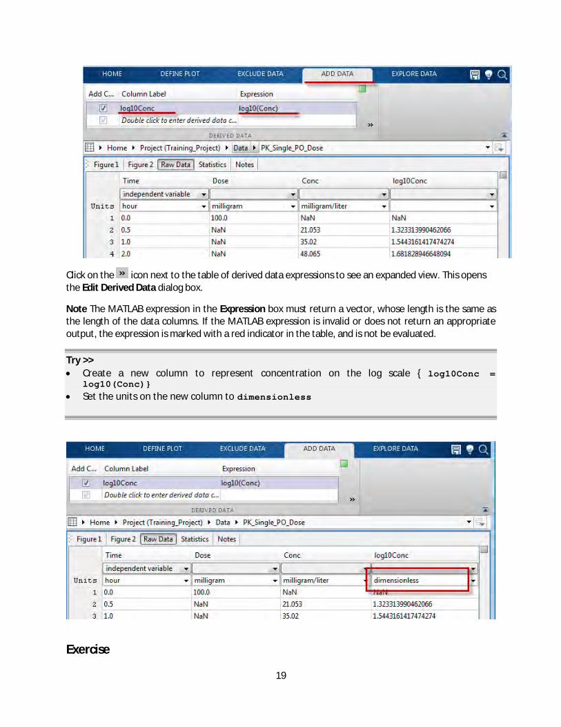
Click on the icon next to the table of derived data expressions to see an expanded view. This opens the Edit Derived Data dialog box.

Note The MATLAB expression in the Expression box must return a vector, whose length is the same as the length of the data columns. If the MATLAB expression is invalid or does not return an appropriate output, the expression is marked with a red indicator in the table, and is not be evaluated.

Try >>

Create a new column to represent concentration on the log scale { log10Conc =

log10(Conc)}

Set the units on the new column to dimensionless

Exercise

20

Import data from PKPD_Oral_Dosing_Data.xlsx file

Rename the imported dataset: PKPD_Single_PO_Dose Configure the units on columns as follows: Time in hour, Dose in milligram, PK in

milligram/liter and PD in milligram

Create the following plots: o Scatter plot of PK vs. Time o Scatter plot of PD vs. Time (create the second plot in a new figure window)

Chapter 4 Parameter Estimation

21


Topics Covered

Parameter estimation (nonlinear regression)

Configuring parameter estimation task

Results and diagnostic plots

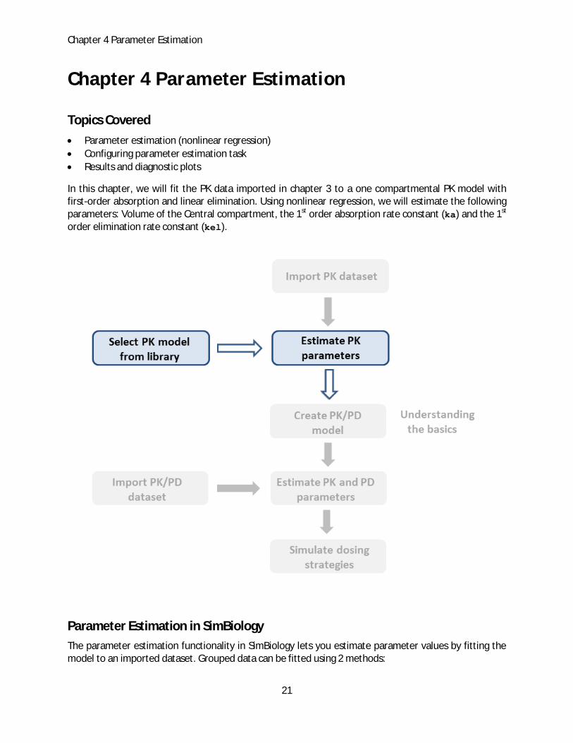
In this chapter, we will fit the PK data imported in chapter 3 to a one compartmental PK model with first-order absorption and linear elimination. Using nonlinear regression, we will estimate the following parameters: Volume of the Central compartment, the 1st order absorption rate constant (ka) and the 1st order elimination rate constant (kel).

Parameter Estimation in SimBiology

The parameter estimation functionality in SimBiology lets you estimate parameter values by fitting the model to an imported dataset. Grouped data can be fitted using 2 methods:


22

Nonlinear regression (individual fitting) – each group in the dataset is independently fit to the model using nonlinear regression (nlinfit)

Nonlinear mixed effects (Population fitting) – the entire dataset is simultaneously fit to the model using nonlinear mixed effects methods (nlmefit & nlmefitsa)

In this chapter, we will cover the nonlinear regression functionality (individual fitting) in SimBiology.

Note The parameter estimation functionality uses features in Statistics Toolbox (Version 7.0 or later).

Adding a Parameter Estimation Task

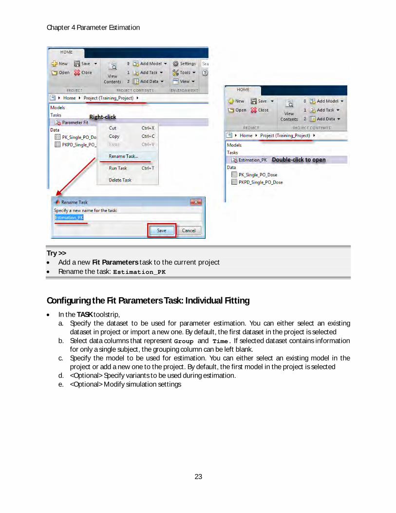
To add a parameter estimation task to the model,

On the HOME tab in the toolstrip, select Add Task > Fit parameters. This adds a new fit task to the project.

To open the task, double-click on the task on the Project or Tasks page. The TASK tab appears in the toolstrip. Click on the tab to configure the task


23

Try >>

Add a new Fit Parameters task to the current project

Rename the task: Estimation_PK

Configuring the Fit Parameters Task: Individual Fitting

In the TASK toolstrip, a. Specify the dataset to be used for parameter estimation. You can either select an existing

dataset in project or import a new one. By default, the first dataset in the project is selected b. Select data columns that represent Group and Time. If selected dataset contains information

for only a single subject, the grouping column can be left blank. c. Specify the model to be used for estimation. You can either select an existing model in the

project or add a new one to the project. By default, the first model in the project is selected d. <Optional> Specify variants to be used during estimation. e. <Optional> Modify simulation settings


24

Once the dataset and model is selected, you can configure the estimation task in the work area. By default, the task panel shows a collapsed, non – editable view of the task configuration. To modify settings, click on [Expand All] link in the upper right corner. [This expands all the tables in the pane.] Alternatively, you can expand or collapse individual information tables using the [Edit] and [Collapse] links next to the tables.

To configure an individual fitting task:

1. Specify the Estimation Method as individual fit (nlinfit) using the pull-down list.

2. Specify the parameters to be estimated. To configure the list of estimable parameters, click on the Edit link. [Opens the table of estimable parameters]. Specify the names of parameters to be estimated under Model Component Name column. The initial estimates of the estimable quantities will be set to the InitialAmount, Value or Capacity of the added Species, Parameter or Compartment, respectively. Modify the values in the Initial Estimate column, if needed. Note If the estimable model component is a species, the initial amount of the species will be estimated; if it is the name of a parameter, the value of the parameter will be estimated; and if it is the name of a compartment, the capacity (or volume) of the compartment will be estimated.

Tip You can drag and drop components from the Component Palette into the Estimated Parameters table. To open the Component Palette, right-click in the Estimated Parameters table and select Show Component Palette

3. If the data contains dosing information, add a dose by clicking on (Add Dose) button in the Dose Information table. For each added dose, specify the dataset column containing the dose information (Dose Column Name), select the dosing type (Type) and map the dosing related columns to the appropriate model components (Dose Component Name, Duration Parameter Name and Time Lag Parameter Name).

4. In the Response Information table, add a response by clicking on the (Add Response) button. For each added response, specify the data column (Column Name) and the model component (Component Name) that it (the selected data column) maps to.


25

5. <Optional> Change the algorithm settings of fitting algorithm under Algorithm Settings.

6. <Optional> Modify the list of plots to be generated at the end of the estimation

7. To run the estimation task, click Run in the TASK toolstrip. [A new results dataset, called Last Run, is added to the project]

Note The minimum data classification required to run the individual fitting task are: (a) independent variable column must be specified, and (b) at least one column must be classified as response, and mapped to an appropriate model component, in the Response Information table.

Try >>

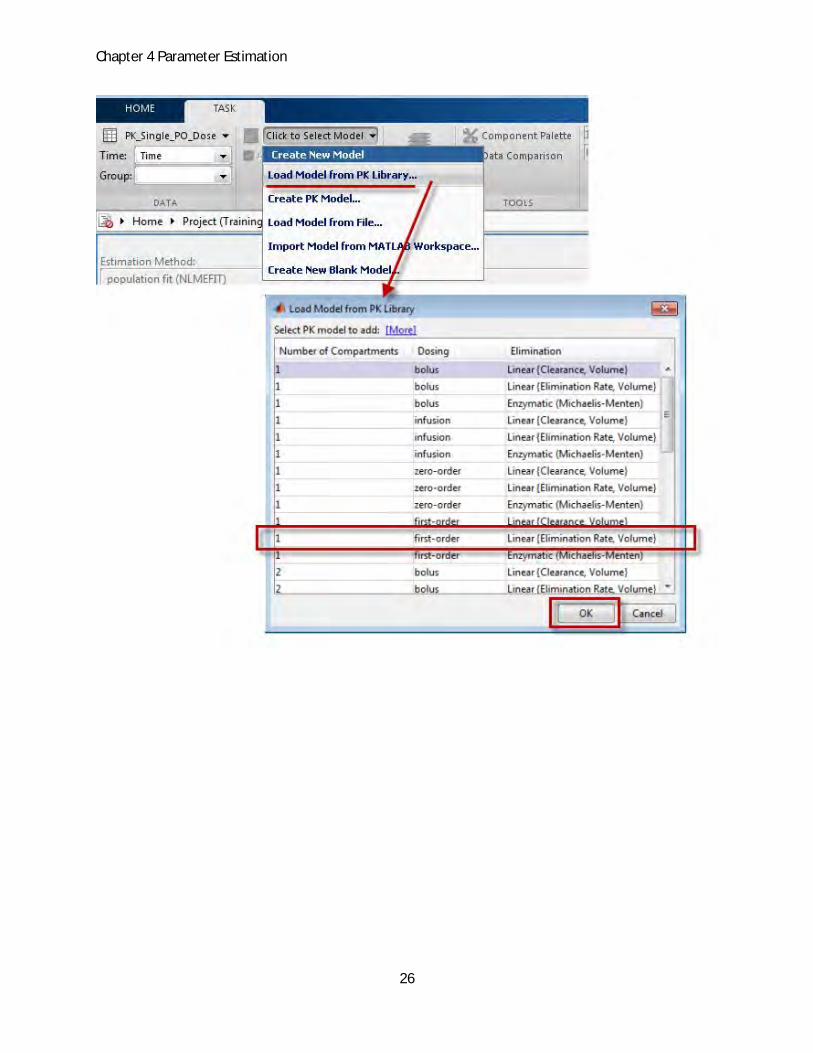
In the estimation TASK tab, choose the PK_Single_PO_Data dataset and a one compartmental model, with first-order dosing with linear elimination. Choose the model from the PK library.

Configure the task to estimate the following parameters: ke_Central and ka_Central, and the volume of the Central compartment. Use 1 as the initial estimates of all 3

parameters.


26


27

Individual Fitting: Results and Diagnostic Plots

The results of the parameter estimation task are stored in a new dataset called Last Run. To open the results of a run:

Double-click on the dataset in the TASK tab (in the TASK RESULTS table). Alternatively, double-click on the dataset on the Project or Data page. [Opens the dataset. The toolstrip displays 2 additional tabs – Define Plot and Explore Data. The work area populates figures generated by the task and a summary tab]


28

The Summary tab in the work area provides the numerical results of the estimation task. This includes the estimates and standard errors on the estimated parameters, and the covariance matrix. The summary task also provides a short summary of the settings and options used to run the task.

The estimation task returns the following plots by defaults.

The predicted time courses and observations for each group

Observed versus predicted values

Residuals versus time, group, or predictions

Distribution of the residuals

A box-plot for individual parameter estimates

In addition to the above default plots, you can add custom plots to the list of plots generated by the fit task.

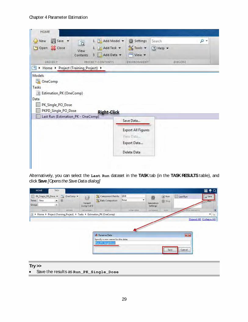
The results saved in the Last Run dataset are overwritten when the task (that generated it) is rerun. To save task results:

On the Project or Data page, right-click on the Last Run dataset and choose Save Data.

Specify the name and click Save. [Renames the dataset]


29

Alternatively, you can select the Last Run dataset in the TASK tab (in the TASK RESULTS table), and click Save [Opens the Save Data dialog]

Try >>

Save the results as Run_PK_Single_Dose


30

Exercise

Add a new Fit Parameters task to the project. Rename the task: Estimation_PKPD

In the estimation task, select the following dataset and model:

o Dataset: PKPD_Single_PO_Dose

o Model : Import PKPD_IDR model from PKPD_IDR_Model.sbproj (Tip Use the Load Model

from File option)

Configure the task as follows:

o Estimation method: individual fit

o Estimated Parameters: ka, ke, EC50, kin, kout and volume of the Central

compartment. Use 1 as the initial estimate on all parameters

o Dose Information: Map data column, Dose, to model component, Central.Dose

o Response Information: Map data columns, PK and PD, to model components, Central.Drug

and PD.Response, respectively.

Save run results as: Run_PKPD_Single_Dose


31

Chapter 5 Modeling: Creating PK Models

32


Topics Covered

MODEL Tab

Creating pharmacokinetic (PK) models

In this chapter, we will learn about creating pharmacokinetic models in SimBiology. First, we will look at the key features of the MODEL tab. Next, we will introduce two methods of adding compartmental PK models in SimBiology: PK Model library and PK Model Wizard.

The MODEL Tab

The MODEL tab is a contextual tab that is visible only when a model is selected in the project. The MODEL tab allows you to view and edit the properties of the model components (we will learn about the details of model components in the next chapter). Broadly speaking, the features on the MODEL tab allow you to:


33

Select a model view

Select and edit model components (in a view-dependent way)

Verify the model

Add and run tasks on the model

The format in which in the model is presented in the work area is dependent on the selected model View. To select a model view:

Open a model, and go on the MODEL tab in the toolstrip

Select a model view under the VIEW list

You can select from one of the following views:

Diagram Shows a graphical representation of the models

Full Shows a list of all components in the model in a single tabular view. The upper panel shows a table of expression (reaction, rules and events) and the lower panel shows a table of quantities (species, compartments and parameters)

Table Shows individual tables of model components

Custom Allows you to combine elements from the Full and Diagram views.


34

Notes

In this tutorial, we will mostly focus on working with the models via the Diagram view.

Some model components (rules, event, doses and variants), are not represented in the Diagram view. Use the Full, Table or Custom views to see or modify these components in the model.

The editing options presented in the MODEL tab are dependent on the selected view. For example, when the Diagram view is selected, the MODEL tabs displays Tools and Scale options to edit the model graphically.

The tasks present in the project, and associated with the model are listed in the Tasks to Run list in the MODEL tab. Double-click on a task to open it. You can also select a particular task and run or edit it.

Try >>

Open the PKPD_IDR model

Change the view to Diagram view

Change the view to Table view - Navigate to the Parameters table. How many parameters in the model? - Navigate to the Species table. How many species in the Central compartment?

Change view to Full view - What are the three types of components listed in the bottom Quantities table?

Creating Pharmacokinetic Models

SimBiology provides you two options to create a compartmental PK model:


35

Choose a model from the PK Library. The library provides compartmental models with up to 3 compartments. Dosing type can be first-order, bolus, infusion or zero-order and elimination route can be either linear or enzymatic.

Creating a model using the PK Wizard. If you want create a compartmental PK model with more than 3 compartments, use the PK Wizard. The wizard allows you to easily create compartmental pharmacokinetic models by specifying the number of compartments and the dosing and elimination routes for each compartment.

To add a PK model from the PK Library:

Select Add Model > Load Model from PK Library in the HOME tab of toolstrip. The Load Model from PK library Model dialog opens.

Select a model

Click OK. This adds a new model to the project

To add a PK model using the PK Wizard:

Select Add Model > Create PK Models in the HOME tab of toolstrip. The Create PK Model dialog opens.

<Optional> Change the Model Name. The default name is untitled.

Specify the Number of Compartments, the Dosing and Elimination type for each compartment. Notice as you change the options, the model schematic in the PK View is updated.

<Optional> Specify if compartment(s) has a measured Response or associated Time Lag.

Click OK. This adds a new model to the project


36

Tip You can also add a model to the project directly from the TASK tab. The model selection tool in the TASK toolstrip gives access to the same options as Add Model.

The PK Wizard and the PK Library provide an easy mechanism to create simple compartmental PK models. Once the model is created, it can be edited or modified like a regular SimBiology model. This will be discussed in detail in the next chapter. Other options for adding a model to the project are:

o Create new blank model to create a custom model o Load model from file to add models from a SimBiology project files or SBML files o Import model from MATLAB workspace to import models from the MATLAB workspace

Chapter 6 Modeling: Creating Custom Models

37


Topics Covered

Understanding the building blocks

Graphically building models

Adding tasks

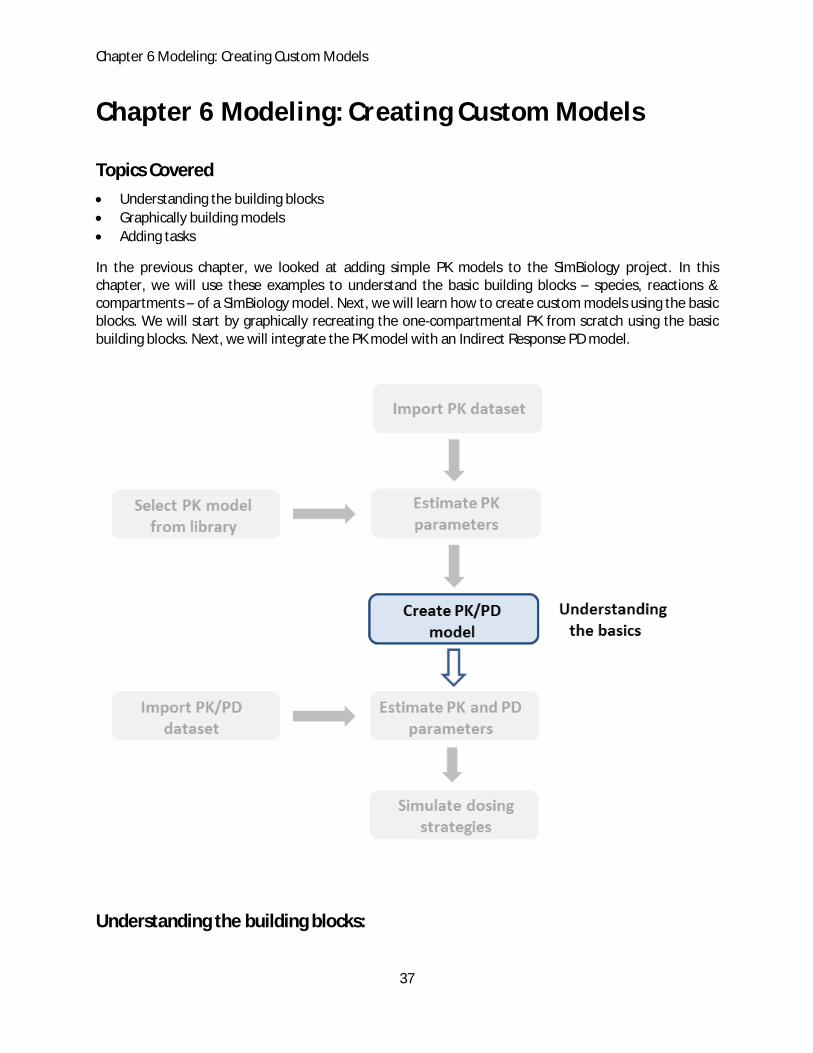
In the previous chapter, we looked at adding simple PK models to the SimBiology project. In this chapter, we will use these examples to understand the basic building blocks – species, reactions & compartments – of a SimBiology model. Next, we will learn how to create custom models using the basic blocks. We will start by graphically recreating the one-compartmental PK from scratch using the basic building blocks. Next, we will integrate the PK model with an Indirect Response PD model.

Understanding the building blocks:


38

SimBiology models are composed of 3 basic building blocks: species, reactions and compartments.

Species represent the state of the model, i.e. the governing equations generated for a SimBiology model describe the dynamics of the amount or concentration of the species (in this case the Drug concentration)

Reactions describe how the species interact with each other, and rate at which they interact (or interconvert). The reaction rate is typically a function of species concentration (or amount) and model parameters. Drug absorption and elimination are represented as reactions in this model.

Compartments represent a well-mixed (homogeneous) container for the species. The capacity of the compartment is used as a scaling factor to convert the species amount into concentration (concentration = amount/capacity), and vice versa.

Note In this document, the term “amount” is loosely used to describe either the amount or the mass of a species. SimBiology recognizes units of both, amount and mass, but it does not have built-in mechanism to interconvert (no way of specifying molecular weight of species).

SimBiology models are translated into a set of coupled ODEs based on mass-balance principles. Typically, there will be one differential equation per species in the model.

The following example illustrates how the above 1-compartmental PK model is translated into ODEs in SimBiology.

Working in the Diagram View

In this chapter, we will mostly focus on working with SimBiology models via the Diagram view. We will briefly switch to the Table view during the discussion on Rules. To see the Diagram view of the model:


Under the VIEW list, select Diagram [Main work area shows a diagrammatic representation of the model]


39

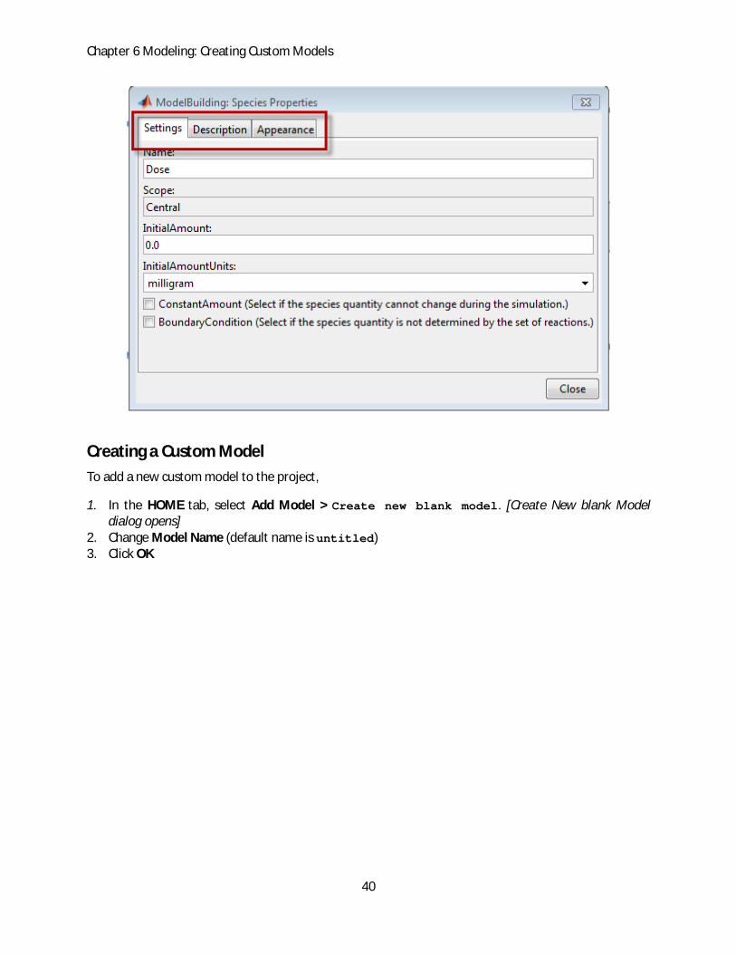
The blocks and lines in the Diagram view are interactive and editable. To access/edit the properties of a block:

Double-click on a block to open the Block Property Editor [Opens block property editor for the selected block.]

View/change any relevant properties

Click Close

The Block Property Editor has 3 tabs: settings, description and appearance. The properties under the settings tab are (mostly) unique to each block type. The appearance and description properties are common across all three block types, i.e., for reaction, species and compartments blocks.


40

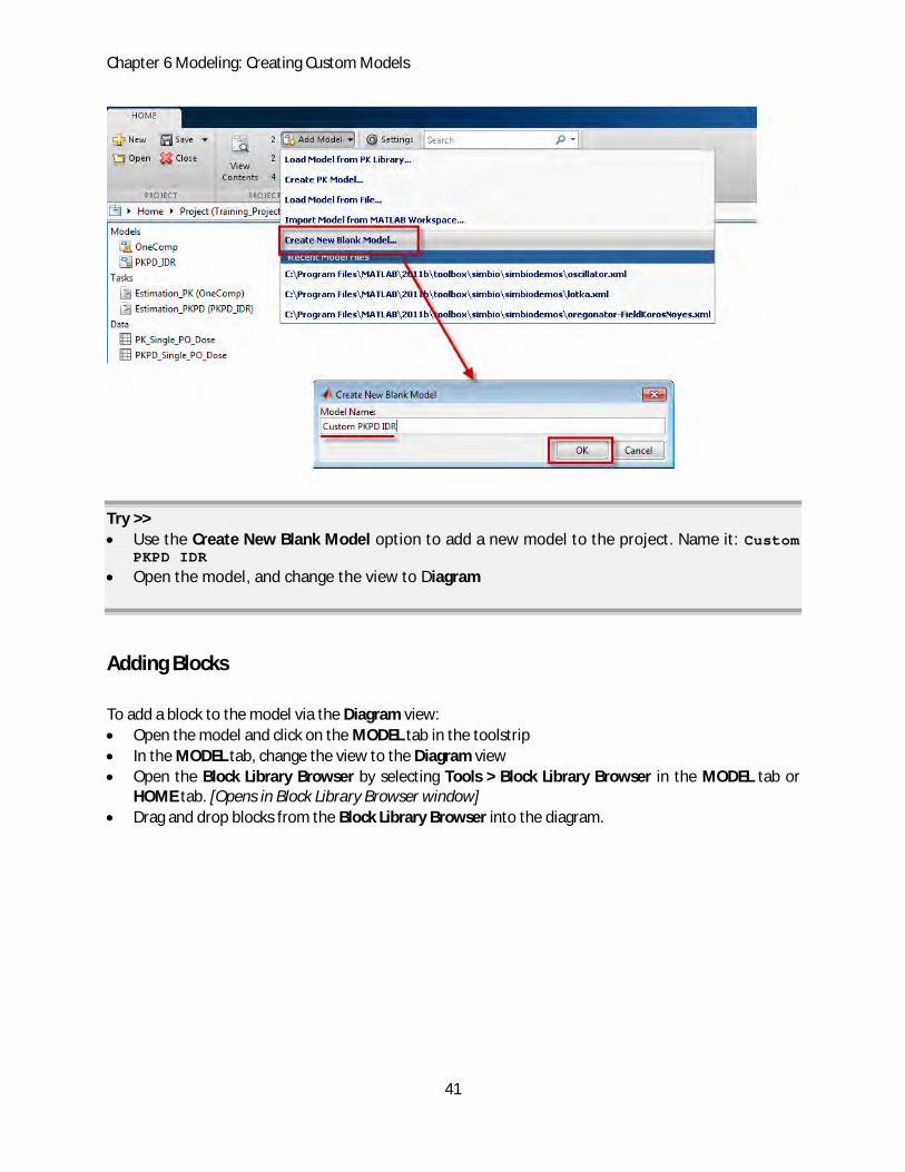
Creating a Custom Model

To add a new custom model to the project,

1. In the HOME tab, select Add Model > Create new blank model. [Create New blank Model dialog opens]

2. Change Model Name (default name is untitled) 3. Click OK


41

Try >>

Use the Create New Blank Model option to add a new model to the project. Name it: Custom PKPD IDR

Open the model, and change the view to Diagram

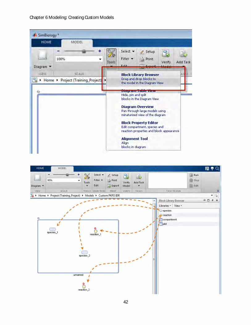
Adding Blocks

To add a block to the model via the Diagram view:

Open the model and click on the MODEL tab in the toolstrip

In the MODEL tab, change the view to the Diagram view

Open the Block Library Browser by selecting Tools > Block Library Browser in the MODEL tab or HOME tab. [Opens in Block Library Browser window]

Drag and drop blocks from the Block Library Browser into the diagram.


42


43

Note In a SimBiology model, species must be scoped to a compartment. When graphically adding species blocks to the diagram, it must be added within an existing compartment block.

Try >> Drag and drop 2 species blocks and 2 reaction blocks into the model diagram

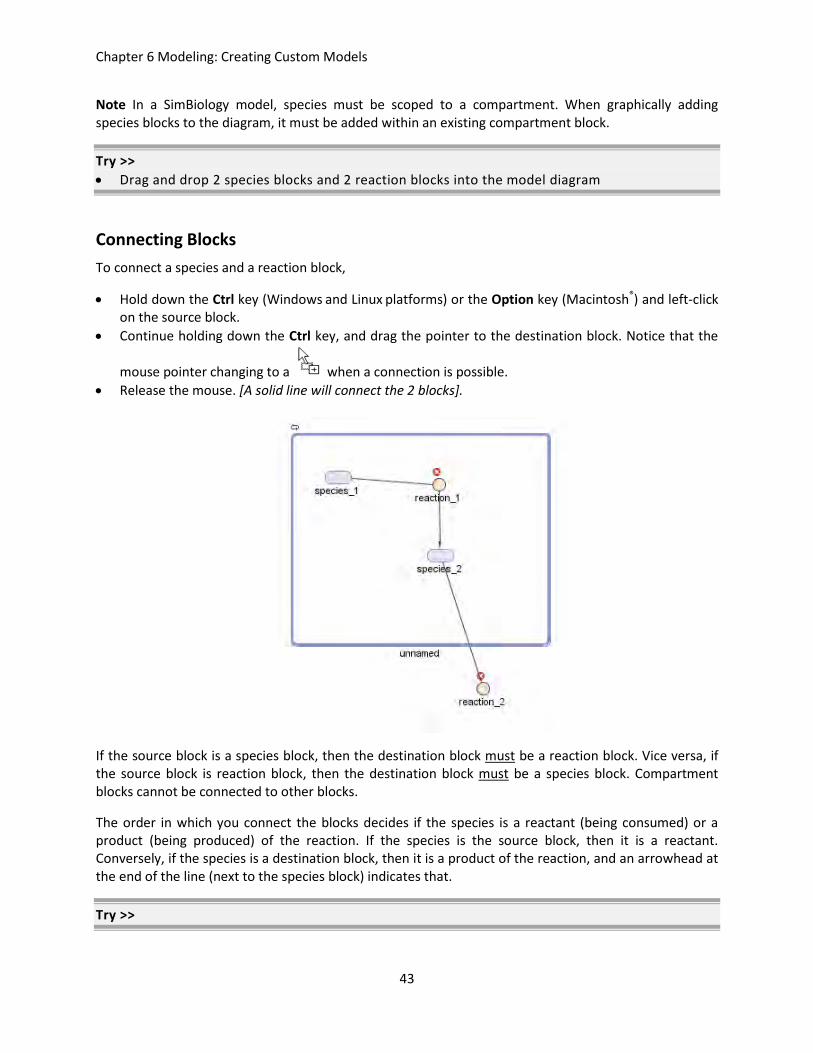
Connecting Blocks To connect a species and a reaction block,

Hold down the Ctrl key (Windows and Linux platforms) or the Option key (Macintosh®) and left-click on the source block.

Continue holding down the Ctrl key, and drag the pointer to the destination block. Notice that the

mouse pointer changing to a when a connection is possible. Release the mouse. [A solid line will connect the 2 blocks].

If the source block is a species block, then the destination block must be a reaction block. Vice versa, if the source block is reaction block, then the destination block must be a species block. Compartment blocks cannot be connected to other blocks.

The order in which you connect the blocks decides if the species is a reactant (being consumed) or a product (being produced) of the reaction. If the species is the source block, then it is a reactant. Conversely, if the species is a destination block, then it is a product of the reaction, and an arrowhead at the end of the line (next to the species block) indicates that.

Try >>


44

Connect the reaction and species blocks such that the species_1 -> species_2 via one reaction block; and species_2 is reactant in the second reaction

Notice the arrowhead next to the species block (species_2) when it is a product of the reaction.

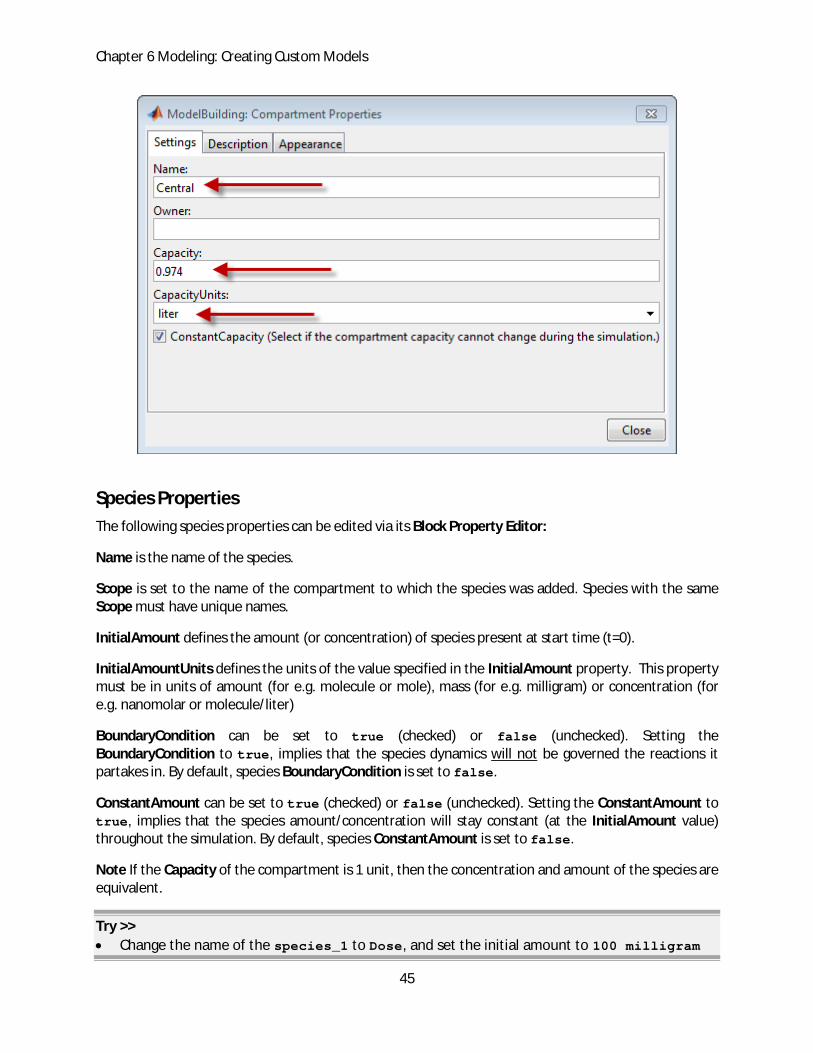
Compartment Properties

The following compartment properties can be edited via its Block Property Editor:

Name is the name of the compartment. Compartment names must be unique, i.e. two compartments in a model cannot have the same name.

Owner is the name of the parent compartment. Compartments blocks can be nested, i.e. a compartment can have a sub-compartment within it. The Owner property is blank for compartment blocks lacking a parent compartment.

Capacity is the scaling factor that translates species amount into concentration. For any species, C = A/V, where C and A are the species concentration and amount, respectively, and V is the Capacity of the compartment to which the species is scoped.

CapacityUnits specifies the units of the Capacity property. Valid units are in dimension of length, area or volume.

ConstantCapacity is set to true by default. Setting this property to false allows you to vary the compartment capacity during simulation (using rule/events).

Try >>

Change the name of the compartment to Central, and set the volume to 0.974 liter


45

Species Properties

The following species properties can be edited via its Block Property Editor:

Name is the name of the species.

Scope is set to the name of the compartment to which the species was added. Species with the same Scope must have unique names.

InitialAmount defines the amount (or concentration) of species present at start time (t=0).

InitialAmountUnits defines the units of the value specified in the InitialAmount property. This property must be in units of amount (for e.g. molecule or mole), mass (for e.g. milligram) or concentration (for e.g. nanomolar or molecule/liter)

BoundaryCondition can be set to true (checked) or false (unchecked). Setting the BoundaryCondition to true, implies that the species dynamics will not be governed the reactions it partakes in. By default, species BoundaryCondition is set to false.

ConstantAmount can be set to true (checked) or false (unchecked). Setting the ConstantAmount to true, implies that the species amount/concentration will stay constant (at the InitialAmount value) throughout the simulation. By default, species ConstantAmount is set to false.

Note If the Capacity of the compartment is 1 unit, then the concentration and amount of the species are equivalent.

Try >>

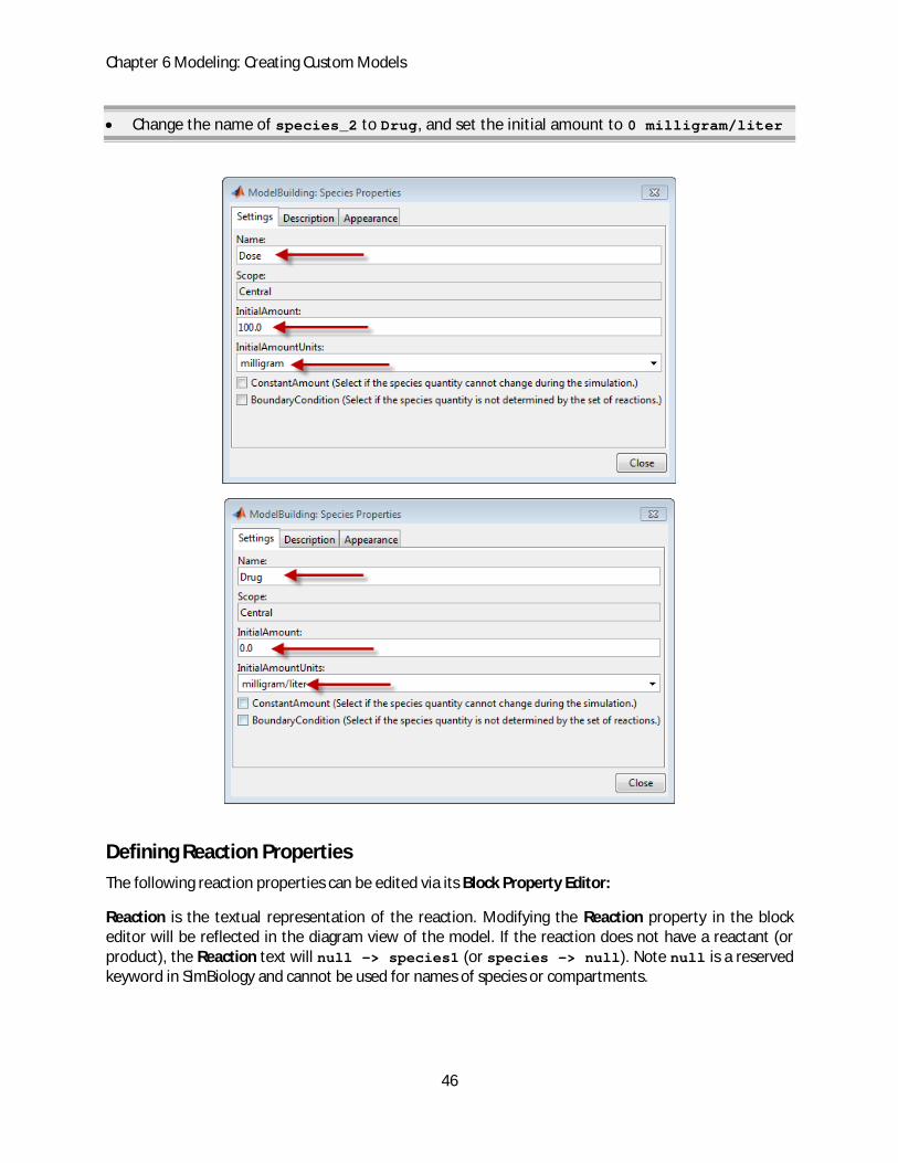
Change the name of the species_1 to Dose, and set the initial amount to 100 milligram


46

Change the name of species_2 to Drug, and set the initial amount to 0 milligram/liter

Defining Reaction Properties

The following reaction properties can be edited via its Block Property Editor:

Reaction is the textual representation of the reaction. Modifying the Reaction property in the block editor will be reflected in the diagram view of the model. If the reaction does not have a reactant (or product), the Reaction text will null -> species1 (or species -> null). Note null is a reserved keyword in SimBiology and cannot be used for names of species or compartments.


47

Reversible is set to false (unchecked) by default. Setting the Reversible property to true makes the reaction a reversible one. This is reflected in the Reaction text ( -> is changed to <-> ) and also in the

diagram view (a icon appears next to the reaction block)

ReactionRate defines how the reaction rate depends on parameter values, species concentrations and compartment volumes. ReactionRate expression can be either manually entered or configured by setting the KineticLaw property.

KineticLaw is the rate law for the reaction. The rate law is a template for constructing the reaction rate expression. The ReactionRate is the result of defining the names of parameters and species variables in a kinetic law.

Active is set to false (unchecked) by default. Setting the Active property to true (checked) excludes

the reaction from the model. Inactive reactions are marked with a ( ) in the diagram.

Name is the name of the reaction

In addition to the above reaction properties, the reaction Block Property Editor also allows you to modify some properties of the quantities (parameters, compartments and species) used in the ReactionRate expression.

Defining Parameter Properties

Parameters have the following properties:

Name is the name of the parameter

Scope is the name of the model or reaction to which the parameter is scoped. To toggle the parameter scope, right-click on the parameter (row) and select Change Parameter Scope. Note: Parameter with the same scope must have unique names.

Value is the value of the parameter

ValueUnits defines the units of the number specified in the parameter Value property

The reaction Block Property Editor lets you modify the property of parameters used in the ReactionRate expression.

Note A yellow indicator appears next to any unused parameters.

Reaction Rate Expressions

Variables used in reaction rate expression must resolve to the name of a species, compartment or a parameter. The rate expression can also use valid MATLAB functions (either built-in or user-defined) that exist on the MATLAB path.

If the rate expression is not correctly configured, a red indicator appears next to the ReactionRate property. To correctly configure unresolved variable names,

Click on the red indicator (opens the Reaction Variables dialog box)


48

Define any unresolved variable names, and click OK

When all variables in the expression are defined, indicator next to the ReactionRate will be green.

If the name of a species used in the expression is not unique, i.e., multiple compartments contain species with the same name, a red indicator will appear next to the ReactionRate expression. Click on the red indicator, and correctly configure the Scope of the species in the Reaction Variables dialog. Alternatively, modify the species name in the expression by adding <compartmentname.> prefix. For example, cell.Receptor or Central.Drug.

To use model components (species, compartments, parameters) whose names contain special characters or space, enclose the name in square brackets. For example, [Receptor*] or [Effect Site]

Try >>

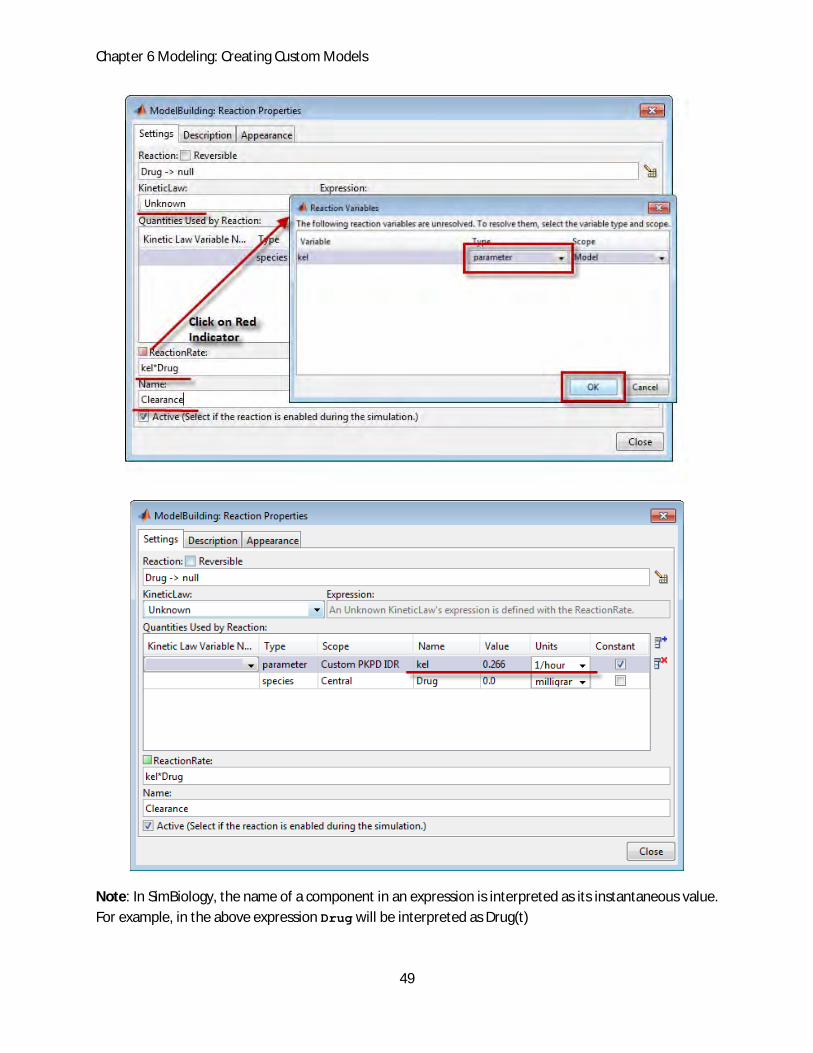
Change name of reaction_1 to Oral Absorption. Set reaction rate as: ka*Dose. Set value of ka = 0.498 1/hour

Change name of reaction_2 to Clearance. Set reaction rate as: kel*Drug. Set value of kel = 0.266 1/hour


49

Note: In SimBiology, the name of a component in an expression is interpreted as its instantaneous value.

For example, in the above expression Drug will be interpreted as Drug(t)


50

Interpretation of Variables in Reaction Rate Expressions

The names of species, parameters and compartments in rate expression are interpreted as follows:

Species Name: If the InitialAmountUnits property of the species is defined, then the species name is interpreted as amount or concentration of the species as decided by its InitialAmountUnits. For example, if the InitialAmountUnits is mole/liter, then the species name will be interpreted as concentration.

If the InitialAmountUnits of the species is not defined, then the species name in the rate expression is interpreted as concentration or amount according to the DefaultSpeciesDimension property (under Simulation Settings). If the DefaultSpeciesDimension is set to substance, the species name is interpreted as the amount of the species, i.e. not scaled by compartment Capacity. If the DefaultSpeciesDimension is set to concentration, the species name is interpreted as the concentration of the species.

DefaultSpeciesDimension property is under Simulation Settings on the TASK tab

Parameter name is interpreted as the Value of the parameter

Compartment name is interpreted as the Capacity of the compartment.

Block Appearance and Description Properties

In addition to species–, compartment– & reaction– specific properties of the blocks, SimBiology blocks also have Appearance and Description properties that can be modified. To view/modify the appearance of a block,

Double-click on the block to open the Block Property Editor.

Click on the Appearance tab, and edit any relevant appearance properties.

Click Close

To resize a block, you can either change the Width and Height under the Appearance properties, or you can click on the block and drag on its corner or edge to resize it.

To modify the description and annotation properties of a block,

Double-click on the block to open the Block Property Editor.

Click on the Description tab, and edit any relevant appearance properties.

Click Close


51

Try >>

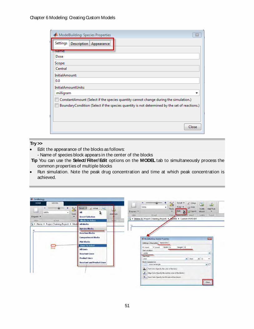
Edit the appearance of the blocks as follows: - Name of species block appears in the center of the blocks

Tip You can use the Select/Filter/Edit options on the MODEL tab to simultaneously process the common properties of multiple blocks

Run simulation. Note the peak drug concentration and time at which peak concentration is achieved.


52

Working with the Table View

In addition to the species, reaction, compartments and parameters described above, SimBiology models can also optionally contain rules and events. Rules and Events, along with the Doses and Variants, are not represented in the model’s Diagram view. To view, modify or modify these components, you need to first change the model view to either Full view or Tables view.

To open the model in the Tables view:


Select the Tables view under the VIEW list


53

Note In this tutorial, we will only discuss the rules construct. You can find more information about Events here

Introduction to Rules

A rule is a mathematical expression that modifies a species amount, compartment capacity, or a parameter value. There are four types of SimBiology rules

algebraic — An algebraic rule is specified as an Expression, and is interpreted as Expression = 0. Algebraic rules are evaluated continuously during simulation, i.e. at each time step of the solver. For example, a mass conservation equation such as Target_Total = Target_Free + Target_Bound where Target_Total is the independent variable, can be written as a rule:

Target_Total - Target_Free + Target_Bound

initialAssignment — An initial assignment rule is specified as Variable = Expression, and is evaluated once at the beginning of a simulation. For example, you could write an initialAssignment rule to set the initial amount of species1 to be proportional to initial amount of species2.

Clearance = kel/Central

repeatedAssignment — a repeated assignment rule is specified as Variable = Expression, and is evaluated continuously during a simulation, , i.e. at each time-step. For example, you could use the following rule to specify that the amount of Drug in the Tissue compartment (Tissue.Drug) is always proportional to the amount of Drug in the Plasma compartment (Plasma.Drug).

Tissue.Drug = P*Plasma.Drug


54

Rate — A rate rule is specified as Variable = Expression, and is interpreted as dVariable/dt = Expression. Rate rules are evaluated continuously during a simulation. For example, to specify dk/dt = 5 (the value of parameter k changes at the rate of 5), write the rate rule as:

k = 5

Notes

Rules overwrite the InitialAmount, Value and Capacity properties for species, parameters and compartments, respectively. For example, if you have an initialAssignment rule, k1 = 5*k2, the value of parameter k1 will be set to 5 times the value of k2 at the start of the simulation, overwriting any number specified in k1's Value property.

If you are using a rule to vary the value (or capacity) of a parameter (or compartment) during simulation, be sure to set its ConstantValue (or ConstantCapacity) property to false.

Adding Rules

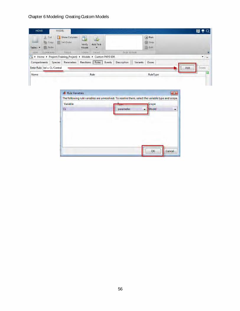
To add a rule,

Open a model, and go on the MODEL tab in the toolstrip. Select the Tables view under the VIEW list

Click on the Rules tab in the work area. The work area displays table of existing rules.

Type the rule expression in the Enter Rule box, and click Add (or press enter). If the expression contains unresolved variables, a Rule Variables dialog will open. Define Type and Scope of unresolved variables and click OK.

Note During simulation, rules are evaluated in the order in which they appear in the rules table. The default order of rules in the table is the sequence in which they were added to the model. To change the order in which the rules are displayed and evaluated:

Left-click on a rule, and drag the mouse pointer to its new position in the table. You can also select multiple rules using the left-click + Shift or left-click+ Ctrl keys.

To set the order of the rules to that displayed in the table, right-click on any rule and select Reorder Rules as Shown in Table. This step is necessary to prevent the order from being reset to the original order.

Rule properties

To edit the properties of a rule, select the rule in the rules table.

Name allows the user to specify (and easily identify) the purpose of the rule. This is an optional property, and can be left blank.

Active is set to true by default. Setting the Active property to false will exclude the rule from the model.

Rule is the mathematical expression that defines the rule.


55

RuleType defines the type of rule to be algebraic, initialAssignment, repeatedAssignment or rate. The rule type decides how the rule expression should be written, and how the expression will be interpreted during simulation. For more information on types of rule, refer to the previous section on Introduction to Rules.

Note From the rules table, you can also edit some properties of parameters, species or compartments used in the rule expression.

Rule Expression

The interpretation of variable names in a rule expression is identical to their interpretation in the reaction rate expressions.

Variables used in rule expression must resolve to the name of a species, compartment or a parameter. The expression can also call valid MATLAB functions (either built-in or user-defined) that exist on the MATLAB path.

If the rule expression is not correctly configured, a red indicator appears next to the Rule expression. To correctly configure unresolved variable names,

Click on the red indicator (opens the Rule Variables dialog box)

Define any unresolved variable names, and click OK

When all variables in the expression are defined, indicator next to the Rule will be green.

If the name of a species used in the expression is not unique, i.e., multiple compartments contain species with the same name, the indicator next to the Rule expression will be red. Click on the red indicator, and correctly configure the Scope of the species in the Rule Variables dialog. Alternatively, prefix the species name in the expression with <compartmentname.>. For example, Cortisol_Site.R1 or Plasma.Drug

To use model components (species, compartments, parameters) whose names contain special characters or space, enclose the name in square brackets, for example, [Receptor*] or [Cortisol Site].

Try >>

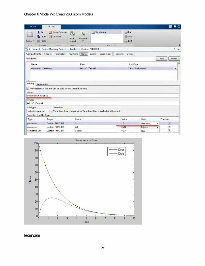
Create a new initial assignment rule that defines the relation between the microscopic elimination rate constant (kel) and the volumetric clearance (CL). - Name the rule: Volumetric Clearance, - Set the rule expression to kel = CL/Central. Set CL = 1 liter/hour.

Run simulation. Note the peak drug concentration and time at which peak concentration is achieved. How does this relate to the values obtained before the addition of the rule?


56


57

Exercise


58

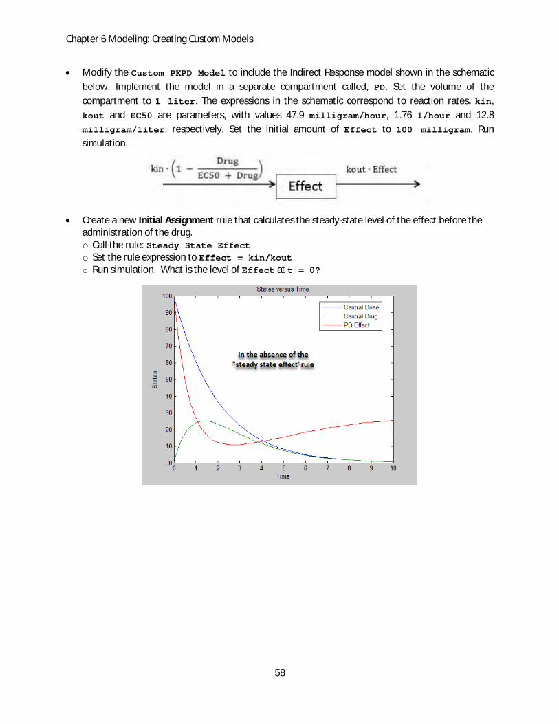
Modify the Custom PKPD Model to include the Indirect Response model shown in the schematic

below. Implement the model in a separate compartment called, PD. Set the volume of the

compartment to 1 liter. The expressions in the schematic correspond to reaction rates. kin,

kout and EC50 are parameters, with values 47.9 milligram/hour, 1.76 1/hour and 12.8

milligram/liter, respectively. Set the initial amount of Effect to 100 milligram. Run

simulation.

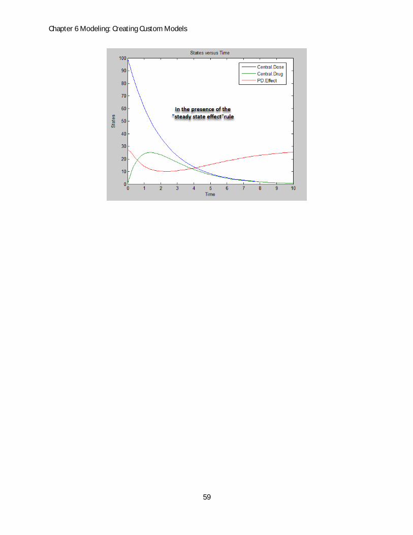
Create a new Initial Assignment rule that calculates the steady-state level of the effect before the administration of the drug. o Call the rule: Steady State Effect o Set the rule expression to Effect = kin/kout o Run simulation. What is the level of Effect at t = 0?


59

60

Chapter 7 Simulating and Analyzing Models

Topics Covered

TASK toolstrip

Modifiers: Doses and Variants

Simulation Settings: Dimensional Analysis and Unit Conversion

Simulation Task

In this chapter, we will introduce some of the built-in tasks that can be performed on SimBiology models. First, we will learn how to add and run tasks on a SimBiology model. Next, we will explore the main navigation features of the TASK tab. Finally, we will specifically look at configuring and running simulations.

61

Adding a Task

To directly add a task to a model:

Open the model and go to the MODEL tab

Click on Add Tasks, and select the task to be added. [Selected task is added to the project, and is listed the Tasks to Run table in the MODEL tab]

Note When you add a task to a model, the task gets added to the project. The model selected on the task is set to the model to which the task was added. Alternatively, you can add a task to the project (using the Add Task option from the HOME tab), and then specify the model to be used in the task.

Running a Task

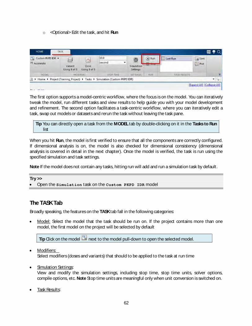
SimBiology provides two ways to run a task:

Option 1: Model-centric workflow o Open the model and go to the MODEL tab o Select a task in the Tasks to Run list in the MODEL tab and click Run

Option 2: Task-centric workflow o Open the task and go to the TASK tab.

62

o <Optional> Edit the task, and hit Run

The first option supports a model-centric workflow, where the focus is on the model. You can iteratively tweak the model, run different tasks and view results to help guide you with your model development and refinement. The second option facilitates a task-centric workflow, where you can iteratively edit a task, swap out models or datasets and rerun the task without leaving the task pane.

Tip You can directly open a task from the MODEL tab by double-clicking on it in the Tasks to Run list

When you hit Run, the model is first verified to ensure that all the components are correctly configured. If dimensional analysis is on, the model is also checked for dimensional consistency (dimensional analysis is covered in detail in the next chapter). Once the model is verified, the task is run using the specified simulation and task settings.

Note If the model does not contain any tasks, hitting run will add and run a simulation task by default.

Try >>

Open the Simulation task on the Custom PKPD IDR model

The TASK Tab

Broadly speaking, the features on the TASK tab fall in the following categories:

Model: Select the model that the task should be run on. If the project contains more than one model, the first model on the project will be selected by default

Tip Click on the model next to the model pull-down to open the selected model.

Modifiers: Select modifiers (doses and variants) that should to be applied to the task at run time

Simulation Settings: View and modify the simulation settings, including stop time, stop time units, solver options, compile options, etc. Note Stop time units are meaningful only when unit conversion is switched on.

Task Results:

63

View the list of saved runs of the task. Click on a dataset in the list to view, save or plot its contents.

Next, we will discuss some of the above features in details.

Modifiers: Doses & Variants

In addition to the model components discussed in the previous chapter, SimBiology provides the following constructs (or objects) that you use to modify or perturb a model from its base configuration.

Doses

The Doses feature in SimBiology allows users to easily create different dosing schedules, and test their effect on model behavior. Doses can be applied to the model at simulation time that enables one to test different dosing options without altering the properties of the base model.

When a dose is applied during a simulation, the value of the dosed component (as specified by TargetName) is appropriately varied during the simulation according to the specified dosing parameters.

Variants

Variants are sets of alternative values for model components that can be applied to the model during simulation. Variants can store values of:

Species InitialAmount

Parameter Value

Compartment Capacity

Applying one or more variants to the model during simulation allows you to evaluate model behavior under different conditions without altering the values in the original model. With the commit option you can easily replace the values of model components with those in the variant, if needed.

When a variant is used in a simulation, the values of model components are temporarily set to those specified in the variant. When multiple variants are used during a simulation, and there are duplicate specifications for a component's value, the last occurrence for the component value in the array of variants is used during simulation

Adding Doses

To add a new dose schedule to a model:

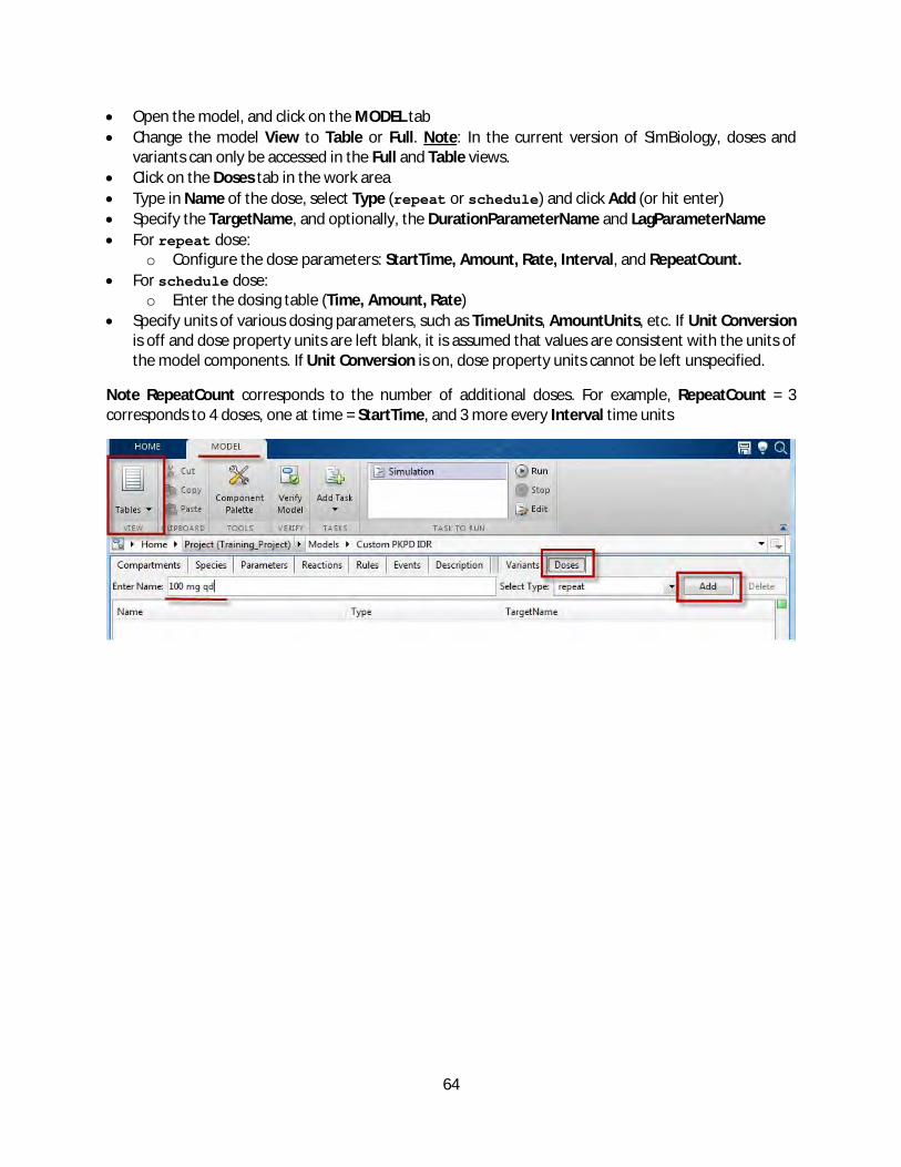
64

Open the model, and click on the MODEL tab

Change the model View to Table or Full. Note: In the current version of SimBiology, doses and variants can only be accessed in the Full and Table views.

Click on the Doses tab in the work area

Type in Name of the dose, select Type (repeat or schedule) and click Add (or hit enter)

Specify the TargetName, and optionally, the DurationParameterName and LagParameterName

For repeat dose: o Configure the dose parameters: StartTime, Amount, Rate, Interval, and RepeatCount.

For schedule dose: o Enter the dosing table (Time, Amount, Rate)

Specify units of various dosing parameters, such as TimeUnits, AmountUnits, etc. If Unit Conversion is off and dose property units are left blank, it is assumed that values are consistent with the units of the model components. If Unit Conversion is on, dose property units cannot be left unspecified.

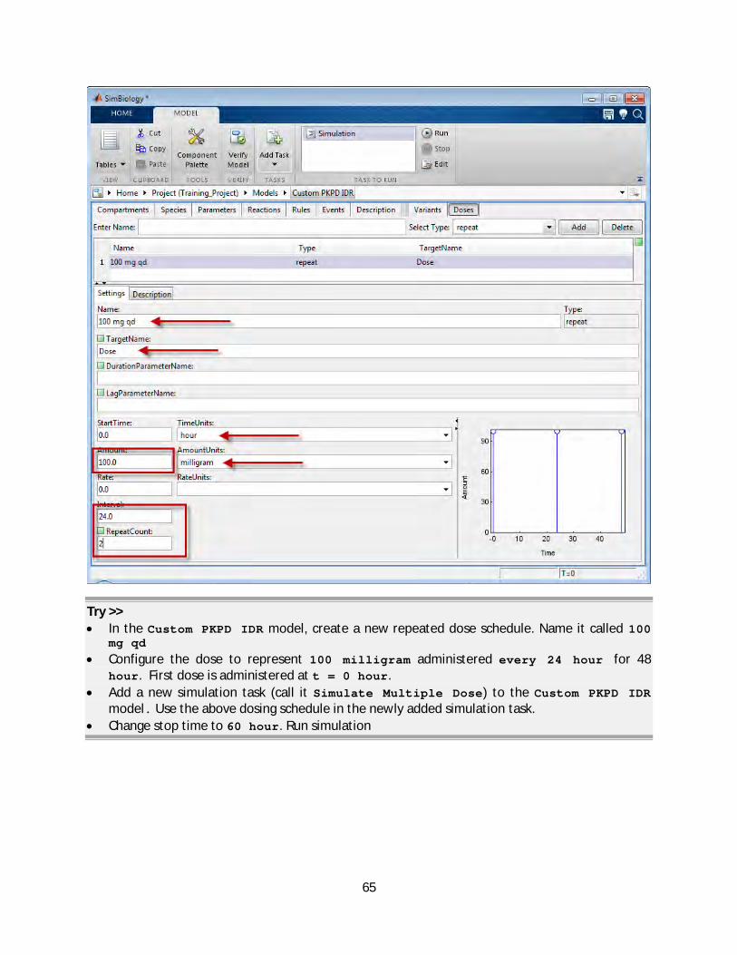
Note RepeatCount corresponds to the number of additional doses. For example, RepeatCount = 3 corresponds to 4 doses, one at time = StartTime, and 3 more every Interval time units

65

Try >>

In the Custom PKPD IDR model, create a new repeated dose schedule. Name it called 100 mg qd

Configure the dose to represent 100 milligram administered every 24 hour for 48 hour. First dose is administered at t = 0 hour.

Add a new simulation task (call it Simulate Multiple Dose) to the Custom PKPD IDR model. Use the above dosing schedule in the newly added simulation task.

Change stop time to 60 hour. Run simulation

66

Adding Variants

To add a new dose schedule to a model:

Open the model, and click on the MODEL tab

Change the model View to Tables or Full. Note: In the current version of SimBiology, doses and variants can only be accessed in the Full and Tables views.

Type in Name of the variant and click Add (or hit enter)

In the Settings pane, select the Type of the component as a Parameter, Species or Compartment.

Enter the Name of the component. Notice that as you start typing the name, a list of components starting with the typed letters appears at the cursor. Continue typing or use the down arrow to select the component.

In the Value cell, type a value of the component for the variant.

You can add more components to the variant, and configure them by repeating the above steps.

Tip You can also create a variant directly from the results dataset of a parameter estimation task. This allows you to create a new variant that stores the values of the estimated parameters.

Using Modifiers in tasks

To use a modifier (doses or variants) in a task:

67

Open the task, and click on the TASK tab Click on Dose (or Variant) button in the TASK tab [Opens the Dose Selection or Variant Selection

dialog] Specify the doses (or variants) to be used in the task by checking their selection boxes. To simulate the task, click Run in the TASK tab

Try >>

In the Custom PKPD IDR model, create a variant that holds the PD parameter values estimated from a different dataset. Name the variant Alternate Drug Efficacy. Set the values of the parameters as follows: EC50 = 0.128 milligram/liter

Use the above variant in the Simulate Multiple Dose task

Run simulation. How does the efficacy profile differ from the previous run?

68

Dimensional Analysis

The dimensional analysis feature in SimBiology checks the model for dimensional consistency prior to simulation. When this feature is on, the model is checked to ensure that the physical quantities of the units involved in expressions match, and are applicable.

To perform dimensional analysis on the model before simulation:

Click on Simulation Settings in the TASK tab. [Opens the Default Simulation Settings window]

Check the DimensionalAnalysis check box under CompileOptions

Dimensional analysis is on by default for new models. When dimensional analysis is on, all model objects that are used in active expressions (rate, rule or event) must have units defined. If one or more units are not defined, dimensional analysis will give a warning

When the dimensional analysis feature is switched on, the model is mainly tested for 2 things:

Reaction rate resolve to units of concentration/time or amount/time. If the physical quantities do not match, the simulation will fail and you see an error.

69

Terms being added, subtracted or equated in any expression (rate, rule or events) are dimensionally consistent. For example, consider a repeated assignment rule species_1 = k1*species2 + x0. If you specify the initial amount of species_1 in milligram, the value of x0 and k1*species2 must also have units of mass. If x0 or k1*species2 resolve to any other dimension, the dimensional analysis will fail and model will not be simulated. (Rules are covered in the next chapter: Advanced Modeling Features

Note If you have MATLAB function calls in your expression, dimensional analysis ignores any expressions containing function calls and generates a warning.

Unit Conversion

The unit conversion feature enables users to specify values of model components (InitialAmount, Value and Capacity) in different unit systems, and the software performs unit conversion to ensure that simulation is performed in a consistent unit system.

To perform unit conversion during simulation,

Click on Simulation Settings in the TASK tab. [Opens the Default Simulation Settings window]

Check the UnitConversion check box under CompileOptions

When UnitConversion is set to true, values are converted to one consistent unit system during simulation. All quantities are reconverted to the user-specified units after simulation. Simulation plots and results will be displayed in the units specified by the user. Simulation time is returned in units specified under StopTime Units

Notes:

Unit conversion cannot be performed if dimensional analysis is off.

70

If unit conversion is off, then the software will assume that the specified values are in consistent unit system and use them as such. In this case, it is the user's responsibility to ensure values are specified in a consistent unit system.

If Unit Conversion is on during parameter estimation, then units must be specified on data columns used in the estimation task. If Unit Conversion is off, then the user must ensure that the units on the data are consistent with each other, and with the units on the model components

Try >>

In the Simulate Multiple Dose task, change stop time to 3600 minute. Run task

Switch on unit conversion and simulate the model. Compare the results with the predicted profile from the previous run.

simbiology for pharmacokinetic and mechanistic modeling · simbiology ® for pharmacokinetic and...

Documents