research article damage localization of cable-supported

Research ArticleDamage Localization of Cable-Supported Bridges Using ModalFrequency Data and Probabilistic Neural Network

X. T. Zhou,1 Y. Q. Ni,2 and F. L. Zhang3

1 The Second Jiaojiang Bridge Construction Headquarters, Jiaojiang, Zhejiang 318000, China2Department of Civil and Environmental Engineering, The Hong Kong Polytechnic University, Hung Hom,Kowloon, Hong Kong

3 Research Institute of Structural Engineering and Disaster Reduction, College of Civil Engineering, Tongji University,Shanghai 200092, China

Correspondence should be addressed to Y. Q. Ni; [email protected]

Received 4 February 2014; Accepted 12 May 2014; Published 2 June 2014

Academic Editor: Hua-Peng Chen

Copyright © 2014 X. T. Zhou et al. This is an open access article distributed under the Creative Commons Attribution License,which permits unrestricted use, distribution, and reproduction in any medium, provided the original work is properly cited.

This paper presents an investigation on using the probabilistic neural network (PNN) for damage localization in the suspensionTsingMa Bridge (TMB) and the cable-stayed Ting Kau Bridge (TKB) from simulated noisy modal data. Because the PNN approachdescribes measurement data in a Bayesian probabilistic framework, it is promising for structural damage detection in noisyconditions. For locating damage on the TMB deck, the main span of the TMB is divided into a number of segments, and damage tothe deck members in a segment is classified as one pattern class. The characteristic ensembles (training samples) for each patternclass are obtained by computing the modal frequency change ratios from a 3D finite element model (FEM) when incurring damageat different members of the same segment and then corrupting the analytical results with random noise. The testing samples fordamage localization are obtained in a similar way except that damage is generated at locations different from the training samples.For damage region/type identification of the TKB, a series of pattern classes are defined to depict different scenarios with damageoccurring at different portions/components. Research efforts have been focused on evaluating the influence of measurement noiselevel on the identification accuracy.

1. Introduction

With the aim of assessing the performance and conditionof built structures, damage identification has gained morepopularity and has been extensively studied in the past twodecades. Visual inspection is a traditional way. However, dueto some limitations, for example, inefficient and expensive, itis difficult to be widely used in large-scale structures such ascable-supported bridges [1]. Damage may be hidden inside astructure or located in inaccessible zones whichmake it invis-ible. Furthermore, some anthropogenic and subjective factorsmay also result in a large variability in visual-based conditionassessment [2]. Consequently, a variety of methods basedon field monitoring data have been developed to performdamage detection. Mehrjoo et al. [3] presented a method toperform damage detection of joints in truss bridges using

a neural network based on backpropagation. Hua et al. [4]developed a method by using the measured changes in cableforces to detect the damage in cable-stayed bridges, whichis made by minimizing the cable force error between themeasurement results and analytical model predictions. Liuand de Roeck [5] proposed a damage detection methodin composite bridges using a damage indicator based onthe local modal curvature and wavelet transform modulusmaxima. A Bayesian probabilistic approach was proposed byYin et al. [6] to perform damage characterization in platestructureswith uncertainty considered.Hilbert-Huang trans-form (HHT) method has been applied in damage detectionby formulating a damage detection index [7]. Xia et al. [8]proposed a reliability-based condition assessmentmethod forin-service bridges with the use of long-term monitoring dataof strain. Recently, Chen and Nagarajaiah [9] formulated a

Hindawi Publishing CorporationMathematical Problems in EngineeringVolume 2014, Article ID 837963, 10 pageshttp://dx.doi.org/10.1155/2014/837963

2 Mathematical Problems in Engineering

detection-filter-based decentralized controller for structuraldamage identification, where the genetic algorithm was usedto determine the observer gain.

Among the existing methods, neural network (NN)method, which can simulate the human decisionmaking anddraw conclusions even when presented with complex infor-mation, has been attracting great attention since it is efficientto look for the similarities among large bodies of data [10–13]. As an important form of NN method, the probabilisticneural network (PNN) can perform the Bayesian decisionanalysis with the Parzen windows estimator cast into anartificial neural network framework. Specht [14] presented adetailed introduction of PNN. In the original PNN, a verylarge network needs to be formed which leads to a highrequirement for the computation and an extensive storage[15]. To make the method more practical and easy to realize,several modified PNNs were developed [16–18]. In the pastseveral years, PNN has been applied in many related fields,for example, eddying current flaw characterization in tubes[19], evaluating seismic liquefaction potential [20], freewayincident detection [21], reliability assessment of oil and gaspipelines [15], diagnosis of prestressed concrete pile defects[22], earthquake magnitude prediction [23], and so on. Sincethe PNN approach describes measurement data in a Bayesianprobabilistic framework, it shows great promise for structuraldamage detection in noisy conditions [24–27].

This paper presents an investigation on using the PNN fordamage localization in cable-supported bridges from noisymeasurement data. Because a cable-supported bridge com-prises at least thousands of structural members, the conven-tional damage detection methods based on optimization andparameter identification is very difficult, if not impossible, tobe implemented for cable-supported bridges [28]. When thePNN is applied to damage identification, it uses exemplarsfrom the undamaged and damaged structure to establishwhether a new measurement of unknown origin comesfrom the undamaged class or the damaged class. In thepresent study, the suspension Tsing Ma Bridge (TMB) andthe cable-stayed Ting Kau Bridge (TKB) in Hong Kong, bothbeing instrumented with online structural health monitoringsystems [29, 30], are considered as “testbeds” for simulationstudies of damage localization using the PNN technique.Precise 3D finite element models (FEMs) of the two cable-supported bridges are first established to perform modalanalysis and damage simulation. In recognizing relativelyhigh uncertainty in measured modal shapes, only modalfrequencies identified from noisy measurement data are usedto construct the input vector in the PNN. On the TMB, thePNN is configured to identify the damaged segment on themain span deck of the bridge through pattern classification.On the TKB, the PNN is configured to consist of patternclasses which are defined by assuming damage at the mainstay cables, longitudinal stabilizing cables, transverse stabi-lizing cables, main girders, cross-girders, and bearings of thebridge, respectively. Different numbers of modal frequenciesare considered to construct input vector to the PNN, andthe effect of different levels of measurement noise containedin the modal frequencies on the identification accuracy isstudied.

2. PNN for Structural Damage Identification

Cast into an artificial neural network, the PNN implementsthe Bayesian decision rule by representing the probabilitydensity functions (PDFs) of the known data sets with anonparametric estimator, then judges which set of knowndata is the most likely source of the unknown datum [14].Since it directly casts the PDFs of training samples in thenetwork, the network configuration of PNN is convenient fordealing with the noisy and series measurement data whenapplied for damage identification. A salient feature of PNNis that it can explicitly accommodate the noise characteristicas neuroweights in the trained network. The Bayes strategyis a widely accepted norm for decision rules used to classifypatterns. For a multicategory classification problem with anumber of categories 𝜃

1, 𝜃2, . . . , 𝜃

𝑞, . . . , 𝜃

𝑠, the Bayes decision

rule to decide the state of nature 𝜃 ∈ 𝜃𝑞based on a set of

measurements represented by a 𝑝-dimensional vector X =

{𝑥1, 𝑥2, . . . , 𝑥

𝑖, . . . , 𝑥

𝑝}𝑇 can be described as

𝑑 (X) ∈ 𝜃𝑞

if ℎ𝑞𝑙𝑞𝑓𝑞(X) > ℎ

𝑘𝑙𝑘𝑓𝑘(X) , ∀𝑘 ̸= 𝑞, (1)

where 𝑑(X) is the decision on test vector X; ℎ𝑞, ℎ𝑘are the a

priori probabilities of the categories 𝜃𝑞and 𝜃𝑘, respectively; 𝑙

𝑞

is the loss associated with misclassifying 𝑑(X) ∉ 𝜃𝑞when 𝜃 ∈

𝜃𝑞and 𝑙𝑘is the loss associated with misclassifying 𝑑(X) ∉ 𝜃

𝑘

when 𝜃 ∈ 𝜃𝑘; 𝑓𝑞(X) and 𝑓

𝑘(X) are the PDFs for categories 𝜃

𝑞

and 𝜃𝑘, respectively.

For the damage detection problem, ℎ and 𝑙 are usuallyassumed to be equal for all categories. Therefore, the key tousing (1) is the ability to estimate PDFs based on trainingpatterns. Here, the method of Parzen windows is used toestimate the PDFs in terms of kernel density estimators [31]:

𝑓𝑞(X) =

1

𝑛𝑞(2𝜋)𝑝/2

𝜎𝑝

𝑛𝑞

∑

𝑖=1

exp[

[

−(X − X

𝑞𝑖)𝑇

(X − X𝑞𝑖)

2𝜎2]

]

,

(2)

whereX is the test vector to be classified; 𝑓𝑞(X) is the value of

the PDF of category 𝑞 at point X; 𝑛𝑞is the number of training

vectors in category 𝑞; 𝑝 is the dimensionality of the trainingvectors; X

𝑞𝑖is the 𝑖th training vector for category 𝑞; 𝜎 is the

smoothing parameter. Equation (2) implies that any smoothdensity function can be expressed simply as the sum of smallmultivariate Gaussian distributions. It is known from (2) thatit is not necessary to calculate the full PDFwhen using Parzenwindows for classification; all that is needed is its value at thetest vector point.

The PNN is designed to cast the Bayesian decision analy-sis with the Parzenwindows estimator into an artificial neuralnetwork configuration. Figure 1 illustrates the architecture ofthe PNN configured for damage localization. It consists ofthree layers: input (distribution) layer, pattern layer, and sum-mation layer. An input vector X = {𝑥

1, 𝑥2, . . . , 𝑥

𝑖, . . . , 𝑥

𝑝}𝑇

to be classified is applied to the neurons of the input layerthat just supply the same input values to all the pattern units.In this study, the input vector is taken as the frequencychange ratios for 𝑝 vibration modes of the structure before

Mathematical Problems in Engineering 3

x1 x2 xi xp

z11 zs1zsn𝑠

Input layer

Pattern layer

Summation layer· · · · · ·

· · · · · ·· · ·

· · · · · ·

O1 Ok Os

z1n1

Figure 1: Architecture of a three-layer PNN.

and after damage. In the pattern layer, each neuron forms adot product of the pattern vector X with the weight vectorW𝑗of a given class, 𝑧

𝑗= X ⋅ W

𝑗, and then performs a

nonlinear operation on 𝑧𝑗before output to the summation

layer. Instead of the sigmoidal activation function commonlyused for backpropagation network, the activation functionused here is 𝑔(𝑧

𝑗) = exp[(𝑧

𝑗− 1)/𝜎

2]. Each neuron in the

summation layer receives all pattern layer outputs associatedwith a given class. For instance, the output of the summationlayer neuron corresponding to the class 𝑞 is

𝑓𝑞(X) =

𝑛𝑞

∑

𝑗=1

𝑧𝑞𝑗

=

𝑛𝑞

∑

𝑗=1

exp[X ⋅W

𝑞𝑗− 1

𝜎2] . (3)

It can be readily proven that if the weight vector W𝑞𝑗

is taken as the training vector X𝑞𝑗

corresponding to theclass 𝑞 and both X and X

𝑞𝑗are normalized with X ⋅ X =

X𝑞𝑗

⋅ X𝑞𝑗

= 1, then the resulting output in the summationlayer neuron, (3), is the same form as (2). That is, the kerneldensity estimators for PDFs have been cast into the PNNby setting the weight vectors as the corresponding trainingvectors. The smoothing parameter 𝜎 in (3) represents thestandard deviation of the Gaussian kernels [14]. It has beenshown that [31] with enough training data, the PNN networkis guaranteed to converge to a Bayesian classifier, despite of anarbitrarily complex relationship between the training vectorsand the classification.

3. Finite Element Modeling andModal Analysis

3.1. TsingMa Bridge (TMB). TheTMB as shown in Figure 2 isa double deck suspension bridge with a main span of 1,377mand a total length of 2,160m. It involves about twenty thou-sand structural members, including the framed elements,deck plates, tower beams and columns, main cables, hang-ers, saddles, bearings, and anchorages. In recognizing thatthe conventional modeling procedure for cable-supportedbridges by approximating the bridge deck as analogous con-tinuous beams or grids is not applicable for accurate damagesimulation studies, a precise 3D FEM of the TMB has beendeveloped for the present study.This model has the followingfeatures: (i) it is comprised of 17,677 elements and 7,375

Table 1: Comparison between computed and measured modalfrequencies of Tsing Ma Bridge (TMB).

Mode type andorder

Computed(Hz)

Measured(Hz)

Difference(%)

Predominantlylateral mode

1st 0.0686 0.070 −2.002nd 0.1611 0.170 −5.243rd 0.2546 0.254 0.244th 0.2820 0.301 −6.34

Predominantlyvertical mode

1st 0.1154 0.114 1.232nd 0.1420 0.133 6.753rd 0.1836 0.187 −1.824th 0.2350 0.249 −5.62

Predominantlytorsional mode

1st 0.2584 0.270 −4.302nd 0.3014 0.324 −6.973rd 0.4942 0.486 1.694th 0.5660 0.587 −3.58

nodes, and the spatial configuration of the original structureremains in the model; (ii) the geometric stiffness of cablesand hangers stemming from the large deflection has beenaccurately accounted for in the model through a nonlinearstatic iteration analysis; and (iii) the mass and stiffness con-tribution of individual structural members is independentlydescribed in the model, so the sensitivity of global and localmodal properties to any structural member can be evaluatedconveniently and accurately. Thus, damage to any structuralmember can be directly and precisely simulated.

Modal analysis is then carried out with the formulatedFEM. Figure 3 shows the distribution ofmodal frequencies ofthe TMB, which are found to be closely spaced.The predictedmodal frequencies of the first 67 modes are less than 1.0Hz.The vibration modes of the TMB include global and localmodes. Most of the global modes are three-dimensionaland have coupled components in three directions, especiallythe lateral bending and torsional modes. The fundamentalmodal frequency of the bridge is as low as 0.069Hz whichcorresponds to the first lateral bending mode with the modeshape as a symmetric half-wave in the main span. Thefirst vertical bending mode, with a frequency of 0.115Hz,is an antisymmetric integral wave in the main span. Table 1provides a comparison between the predicted and measuredmodal frequencies for the first four (predominantly) lateral,vertical, and torsional modes, where the measurement datawere obtained by the structural health monitoring systempermanently installed on the bridge [28]. The maximum rel-ative difference between the predicted and measured modalfrequencies for the 16 modes is 6.97%.


1377 m355.5 m76.5 m23 m 300 m72 m 72 m 72 m 72 m

Anchorage Tsing Yi island AnchorageMa Wan island

Ma Wan tower

78.58 m

Tsing Yi tower206.4 m 206.4 m

Figure 2: Elevation of Tsing Ma Bridge (TMB).

0.0

0.2

0.4

0.6

0.8

1.0

1.2

0 20 40 60 80

Frequency order

Freq

uenc

y (H

z)

Figure 3: Distribution of modal frequencies of Tsing Ma Bridge(TMB).

Table 2: Comparison between computed and measured modalfrequencies of Ting Kau Bridge (TKB).

Mode type andorder

Computed(Hz)

Measured(Hz)

Difference(%)

Predominantlyvertical mode

1st 0.1632 0.1618 0.862nd 0.3002 0.3145 −4.553rd 0.3439 0.3527 −2.504th 0.3701 0.3727 −0.70

Predominantlylateral mode

1st 0.1635 — —2nd 0.2236 0.2264 −1.243rd 0.2425 0.2518 −3.694th 0.2477 0.2591 −4.40

Predominantlytorsional mode

1st 0.4587 0.4427 3.612nd 0.5137 0.4809 6.823rd 0.5201 0.5155 0.894th 0.5655 0.5345 5.80

3.2. Ting Kau Bridge (TKB). The TKB as shown in Figure 4is a cable-stayed bridge with two main spans of 448m and475m, respectively, and two side spans of 127m each. TheTKB has three single-leg towers supporting the deck. The

critical problem of a multispan cable-stayed bridge is thestabilization of the central tower. Therefore, longitudinalstabilizing cables, with the length up to 464.6m, are installedto stabilize the central tower. To reduce the vibration of thelongitudinal stabilizing cables, damping devices are installedadjacent to the lower supporting ends of the longitudinalstabilizing cables. Transverse stabilizing cables are also usedto strengthen each tower in sway direction. The deck com-prises two carriageways, which are connected by I-shapecross-girders. Each carriageway grillage is composed of twolongitudinal girders and a series of transverse girders at 4.5mintervals. Girders have been topped by the precast concretedeck panel. There are four main cable planes in the TKB insupporting the carriageways.

A precise 3D FEM containing 5,581 elements and 2,901nodes has been formulated for the TKB, in which the eightlongitudinal stabilizing cables are modeled by multielementcable system, while the remaining 448 cables are modeledby single-element cable system. Modal analysis is then con-ducted with this model, from which it is found that the pre-dicted modal frequencies of the first 125 modes are less than1.05Hz. The modal frequencies are closely spaced as shownin Figure 5. The first mode with a frequency of 0.1632Hz ischaracterized by vertical motion of the deck, longitudinalbending of the central tower, and in-plane vibration of thelongitudinal stabilizing cables. The vibration modes of theTKB can be classified into five categories: (i) global verticalbending modes, (ii) global lateral bending modes, (iii) globaltorsional modes, (iv) cable local out-of-plane modes, and(v) cable local in-plane modes. The first three categoriesare global modes, and the latter two are local modes of thelongitudinal stabilizing cables. It is noted that all the globalmodes are accompanied with local vibration components ofthe cables to some extent. Table 2 provides a comparisonbetween the predicted and measured modal frequencies forthe first four (predominantly) vertical, lateral, and torsionalmodes of the TKB.Themaximum relative difference betweenthe predicted and measured modal frequencies for the 16modes is 6.82%.

4. Damage Localization ofTsing Ma Bridge (TMB)

4.1. Generation of Training and Testing Samples. Numericalsimulation study of damage localization using the PNN is firstmade on the TMB deck. The bridge main span is composed


Ting Kau tower173.530

Ting Kau region

±0.000 ±0.000

Central tower201.450

Tsing Yi region

Tsing Yi tower164.740

Central region

127.0 m 448.0 m 475.0 m 127.0m

Figure 4: Elevation of Ting Kau Bridge (TKB).

Table 3: Training and testing samples for Tsing Ma Bridge (TMB).

Pattern classnumber 1 2 3 4 5 6 7 8 9 10 11 12 13 14 15 16

Deck unitsinvolved 1–4 5–9 10–14 15–19 20–24 25–29 30–34 35–38 39–42 43–47 48–52 53–57 58–62 63–67 68–72 73–76

Training samplesLocation 2, 4 7, 8 10, 12 15, 17 20, 22 25, 27 30, 32 36, 38 39, 41 43, 45 48, 50 53, 55 58, 60 63, 65 68, 70 73, 75Data length 50 × 2 50 × 2 50 × 2 50 × 2 50 × 2 50 × 2 50 × 2 50 × 2 50 × 2 50 × 2 50 × 2 50 × 2 50 × 2 50 × 2 50 × 2 50 × 2

Testing samplesLocation 3 6 11 16 21 26 31 37 40 44 49 54 59 64 69 74Data length 200 200 200 200 200 200 200 200 200 200 200 200 200 200 200 200

0.4

0.8

1.2

1.6

0

0 60 120 180 240

Mode order

Freq

uenc

y (H

z)

Figure 5: Distribution of modal frequencies of Ting Kau Bridge(TKB).

of 76 deck units. To facilitate the damage localization, themain span deck is divided into 16 segments (each including4 or 5 deck units) as listed in Table 3. The damage to thedeck members within the same segment is classified as onepattern class. As a result, there are totally 16 pattern classes;that is, 𝑠 = 16. Because the modal frequencies can beeasily and accurately measured, in this study each patternclass is characterized by the modal frequency change ratiosbetween the undamaged and damaged states. That is, themodal frequency change ratios are used as the entries of theinput vector X = {𝑥

1, 𝑥2, . . . , 𝑥

𝑖, . . . , 𝑥

𝑝}𝑇. The input vector

is designed to comprise the modal frequency change ratiosfor the first 20 modes; that is, 𝑝 = 20. In order to obtain the

training vectors, for each pattern class two damage scenarioswith the damage at different units of the same segment (asshown in Table 3) are introduced in the FEM respectivelyand the modal properties are evaluated accordingly. For eachscenario, the damage is assumed to occur at deckmembers onthe same deck cross-section (for the damage incurred at deckmembers, the maximum modal frequency change is about0.71% among the 20 modes concerned). When the analyticalmodal frequency change ratios for each damage scenario areobtained, they are added with a random sequence to form thetraining vectors

𝑥𝑖= 𝑥𝑎

𝑖× (1 + 𝜀𝑅) , (4)

where 𝑥𝑖is a component of the noise polluted training vec-

tors; 𝑥𝑎𝑖is the analytically computed modal frequency change

ratio for a specific pattern class; 𝑅 is a normally distributedrandom variable with zero mean and unity variance; and 𝜀 isan index representing the noise level.

50 sets of modal frequency change ratios are randomlyproduced for each damage scenario. There are therefore 50 ×

2 = 100 sets of training vectors for each pattern class; thatis, 𝑛1

= 𝑛2

= ⋅ ⋅ ⋅ = 𝑛16

= 100. The number of neurons inthe pattern layer is∑𝑠

𝑘=1𝑛𝑘= 100 × 16 = 1600. After entering

the noise-polluted training vectors of all pattern classes to theinput layer, the PNN for damage localization is trained.Whenpresenting on themanew input vector (test vector) consistingof measured modal frequency change ratios of unknownsource, the configured PNN outputs in the summation layerthe PDF estimates for each pattern class at the test vector


Table 4: Summary of correct identification for Tsing Ma Bridge (TMB).

Pattern classnumber 1 2 3 4 5 6 7 8 9 10 11 12 13 14 15 16 IA ratio (%)Testing samplenumber 200 200 200 200 200 200 200 200 200 200 200 200 200 200 200 200

Number of correctidentification

𝜀 = 100% 23 193 27 49 68 0 6 106 42 65 86 7 31 69 38 31 26.28𝜀 = 90% 38 121 25 50 75 36 45 143 85 36 81 36 54 99 134 56 34.81𝜀 = 80% 55 161 70 62 91 100 68 156 81 55 55 0 55 84 130 21 38.88𝜀 = 70% 31 189 104 62 31 28 49 157 95 63 113 118 92 57 88 60 41.78𝜀 = 60% 50 200 89 97 98 75 105 174 126 60 103 110 89 135 79 80 52.19𝜀 = 50% 92 183 118 115 86 67 79 192 119 123 133 146 113 128 129 110 60.41𝜀 = 40% 123 188 146 133 107 95 147 200 148 123 160 134 123 166 137 111 70.03𝜀 = 30% 164 199 181 164 139 143 183 200 169 170 180 186 180 193 125 111 83.97𝜀 = 20% 186 200 199 198 192 179 197 200 196 189 198 198 192 198 142 173 94.91𝜀 = 10% 200 200 200 200 200 200 200 200 200 200 200 200 200 200 181 197 99.31

Table 5: Simulated damage cases for Ting Kau Bridge (TKB).

Damagetypenumber

Patternclass

numberDescription of damage

11 Damage of longitudinal stabilizing cables

(Ting Kau main span)

2 Damage of longitudinal stabilizing cables(Tsing Yi main span)

2

3 Damage of main stay cables (Ting KauRegion)

4 Damage of main stay cables (CentralRegion)

5 Damage of main stay cables (Tsing YiRegion)

3

6 Damage of transverse stabilizing cables(Ting Kau Region)

7 Damage of transverse stabilizing cables(Central Region)

8 Damage of transverse stabilizing cables(Tsing Yi Region)

49 Damage of bearings (Ting Kau Region)10 Damage of bearings (Central Region)11 Damage of bearings (Tsing Yi Region)

512 Damage of main girders (Ting Kau Region)13 Damage of main girders (Central Region)14 Damage of main girders (Tsing Yi Region)

6

15 Damage of connecting cross-girders (TingKau Region)

16 Damage of connecting cross-girders(Central Region)

17 Damage of connecting cross-girders (TsingYi Region)

point, and the damaged deck segment is identified by thepattern class with the largest PDF.

The test vectors for damage localization simulation studyare produced in a similar way to obtaining the trainingsamples. A total of 16 damage scenarios, with one for eachdeck segment (pattern class), are examined in the simulatedtesting. As shown in Table 3, the testing damage scenariofor each pattern class is incurred at a deck unit differentfrom the corresponding training damage scenarios. Theanalytical modal frequency change ratios when incurringdamage at each deck segment in turn are calculated and thenpolluted with random noise to obtain the “measured” testvectors. The random noise sequences used to contaminatethe training samples and the testing samples are independentbut with identical level in statistical sense. For each testingdamage scenario, 200 sets of noise-corrupted test vectors areproduced. Therefore, a total of 200 × 16 = 3200 test vectorsare used in the damage localization testing.

4.2. Identification Results Using PNN. The configured PNNis applied to the test vectors for damage localization of theTMB. Because the PNN describes the data in a probabilisticapproach, the identification accuracy should be evaluatedin a statistical manner. Table 4 lists the number of correctidentification and the identification accuracy (IA) results forthe total 3200 testing samples by using the PNN. Here thevalue of 𝜀, which represents the noise level, is taken from 0.1to 1.0. The IA is defined as the ratio of the total number ofcorrect identification for all testing damage scenarios to thetotal number of the testing samples (3200). It is seen fromTable 4 that when 𝜀 ≤ 0.2, the PNN can identify the damagesegment with relatively high confidence (IA > 90%).

5. Damage Localization ofTing Kau Bridge (TKB)

5.1. Generation of Training and Testing Samples. Numericalsimulation study is then carried out on using the PNN toidentify damage type and region in the TKB. As listed in


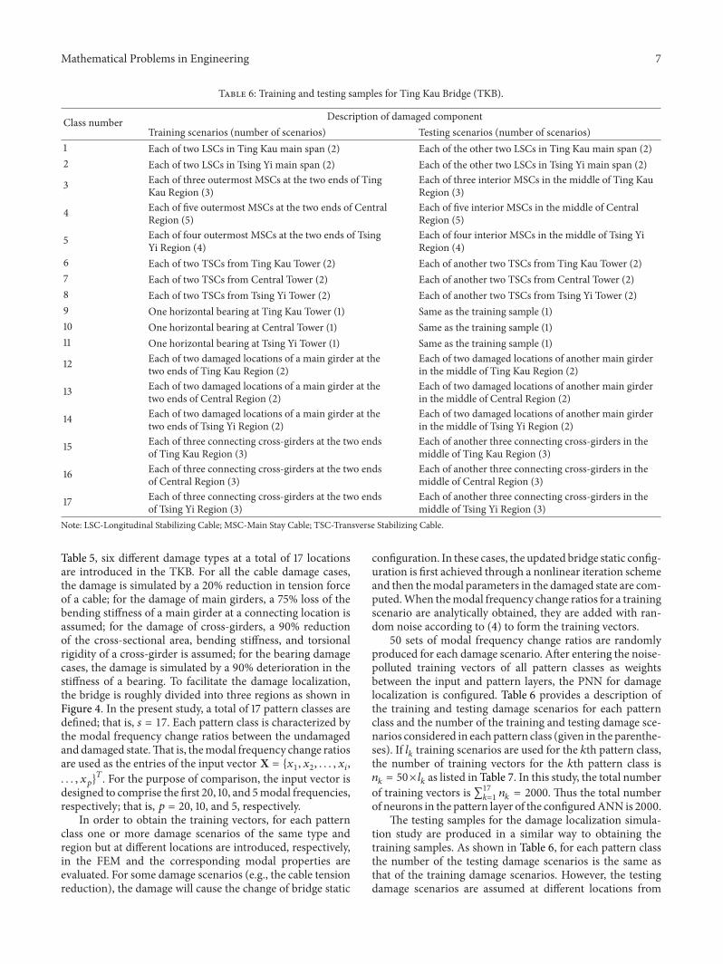
Table 6: Training and testing samples for Ting Kau Bridge (TKB).

Class number Description of damaged componentTraining scenarios (number of scenarios) Testing scenarios (number of scenarios)

1 Each of two LSCs in Ting Kau main span (2) Each of the other two LSCs in Ting Kau main span (2)2 Each of two LSCs in Tsing Yi main span (2) Each of the other two LSCs in Tsing Yi main span (2)

3 Each of three outermost MSCs at the two ends of TingKau Region (3)

Each of three interior MSCs in the middle of Ting KauRegion (3)

4 Each of five outermost MSCs at the two ends of CentralRegion (5)

Each of five interior MSCs in the middle of CentralRegion (5)

5 Each of four outermost MSCs at the two ends of TsingYi Region (4)

Each of four interior MSCs in the middle of Tsing YiRegion (4)

6 Each of two TSCs from Ting Kau Tower (2) Each of another two TSCs from Ting Kau Tower (2)7 Each of two TSCs from Central Tower (2) Each of another two TSCs from Central Tower (2)8 Each of two TSCs from Tsing Yi Tower (2) Each of another two TSCs from Tsing Yi Tower (2)9 One horizontal bearing at Ting Kau Tower (1) Same as the training sample (1)10 One horizontal bearing at Central Tower (1) Same as the training sample (1)11 One horizontal bearing at Tsing Yi Tower (1) Same as the training sample (1)

12 Each of two damaged locations of a main girder at thetwo ends of Ting Kau Region (2)

Each of two damaged locations of another main girderin the middle of Ting Kau Region (2)

13 Each of two damaged locations of a main girder at thetwo ends of Central Region (2)

Each of two damaged locations of another main girderin the middle of Central Region (2)

14 Each of two damaged locations of a main girder at thetwo ends of Tsing Yi Region (2)

Each of two damaged locations of another main girderin the middle of Tsing Yi Region (2)

15 Each of three connecting cross-girders at the two endsof Ting Kau Region (3)

Each of another three connecting cross-girders in themiddle of Ting Kau Region (3)

16 Each of three connecting cross-girders at the two endsof Central Region (3)

Each of another three connecting cross-girders in themiddle of Central Region (3)

17 Each of three connecting cross-girders at the two endsof Tsing Yi Region (3)

Each of another three connecting cross-girders in themiddle of Tsing Yi Region (3)

Note: LSC-Longitudinal Stabilizing Cable; MSC-Main Stay Cable; TSC-Transverse Stabilizing Cable.

Table 5, six different damage types at a total of 17 locationsare introduced in the TKB. For all the cable damage cases,the damage is simulated by a 20% reduction in tension forceof a cable; for the damage of main girders, a 75% loss of thebending stiffness of a main girder at a connecting location isassumed; for the damage of cross-girders, a 90% reductionof the cross-sectional area, bending stiffness, and torsionalrigidity of a cross-girder is assumed; for the bearing damagecases, the damage is simulated by a 90% deterioration in thestiffness of a bearing. To facilitate the damage localization,the bridge is roughly divided into three regions as shown inFigure 4. In the present study, a total of 17 pattern classes aredefined; that is, 𝑠 = 17. Each pattern class is characterized bythe modal frequency change ratios between the undamagedanddamaged state.That is, themodal frequency change ratiosare used as the entries of the input vector X = {𝑥

1, 𝑥2, . . . , 𝑥

𝑖,

. . . , 𝑥𝑝}𝑇. For the purpose of comparison, the input vector is

designed to comprise the first 20, 10, and 5modal frequencies,respectively; that is, 𝑝 = 20, 10, and 5, respectively.

In order to obtain the training vectors, for each patternclass one or more damage scenarios of the same type andregion but at different locations are introduced, respectively,in the FEM and the corresponding modal properties areevaluated. For some damage scenarios (e.g., the cable tensionreduction), the damage will cause the change of bridge static

configuration. In these cases, the updated bridge static config-uration is first achieved through a nonlinear iteration schemeand then themodal parameters in the damaged state are com-puted.When themodal frequency change ratios for a trainingscenario are analytically obtained, they are added with ran-dom noise according to (4) to form the training vectors.

50 sets of modal frequency change ratios are randomlyproduced for each damage scenario. After entering the noise-polluted training vectors of all pattern classes as weightsbetween the input and pattern layers, the PNN for damagelocalization is configured. Table 6 provides a description ofthe training and testing damage scenarios for each patternclass and the number of the training and testing damage sce-narios considered in each pattern class (given in the parenthe-ses). If 𝑙

𝑘training scenarios are used for the 𝑘th pattern class,

the number of training vectors for the 𝑘th pattern class is𝑛𝑘= 50×𝑙

𝑘as listed in Table 7. In this study, the total number

of training vectors is ∑17𝑘=1

𝑛𝑘= 2000. Thus the total number

of neurons in the pattern layer of the configuredANN is 2000.The testing samples for the damage localization simula-

tion study are produced in a similar way to obtaining thetraining samples. As shown in Table 6, for each pattern classthe number of the testing damage scenarios is the same asthat of the training damage scenarios. However, the testingdamage scenarios are assumed at different locations from


Table7:Num

bero

ftrainingandtestingsamples.

Patte

rncla

ssnu

mber

12

34

56

78

910

1112

1314

1516

17

Training

samples

𝑛1=

50×2

𝑛2=

50×2

𝑛3=

50×3

𝑛4=

50×5

𝑛5=

50×4

𝑛6=

50×2

𝑛7=

50×2

𝑛8=

50×2

𝑛9=

50×1

𝑛10=

50×1

𝑛11=

50×1

𝑛12=

50×2

𝑛13=

50×2

𝑛14=

50×2

𝑛15=

50×3

𝑛16=

50×3

𝑛17=

50×3

Total

2000

Testing

samples

𝑚1=

100×2

𝑚2=

100×2

𝑚3=

100×3

𝑚4=

100×5

𝑚5=

100×4

𝑚6=

100×2

𝑚7=

100×2

𝑚8=

100×2

𝑚9=

100×1

𝑚10=

100×1

𝑚11=

100×1

𝑚12=

100×2

𝑚13=

100×2

𝑚14=

100×2

𝑚15=

100×3

𝑚16=

100×3

𝑚17=

100×3

Total

4000


Table 8: Summary of correct identification for Ting Kau Bridge(TKB).

Noise levelIdentification accuracy (IA)

Using 20frequencies

Using 10frequencies

Using 5frequencies

𝜀 = 100% 46.23% 33.35% 27.90%𝜀 = 80% 57.08% 45.25% 33.05%𝜀 = 60% 62.55% 51.85% 43.40%𝜀 = 40% 78.15% 62.90% 51.33%𝜀 = 20% 84.33% 71.70% 58.75%𝜀 = 10% 86.42% 73.53% 60.83%𝜀 = 8% 87.63% 75.08% 63.15%𝜀 = 6% 88.90% 76.85% 65.80%𝜀 = 4% 89.32% 77.23% 67.58%𝜀 = 2% 89.97% 77.35% 67.33%𝜀 = 1% 90.00% 80.05% 67.70%Note: IA (identification accuracy) is defined as the ratio of total number ofcorrect identification to total number of testing samples (4000).

those of the training damage scenarioswithin the same regionof the same type. The analytical modal frequency changeratios for each testing damage scenario are calculated andthen polluted with random noise to obtain the “measured”testing vectors.The random noise sequences used to contam-inate the training samples and the testing samples are inde-pendent but with identical level in statistical sense. For eachtesting damage scenario, 100 sets of noise-corrupted testingvectors are produced.Thus a total of 4000 sets of “measured”testing vectors for 40 testing damage scenarios are obtained.When presenting each set of the testing vectors of “unknown”source to the configured PNN, the PNN outputs in thesummation layer the PDF estimates for each pattern class atthe testing vector point, and the damage type and region areidentified from the pattern class with the largest PDF.

5.2. Identification Results Using PNN. By entering the 4000sets of “measured” testing vectors into the configured PNNin turn, the damage type and region corresponding to eachset of the testing vectors are identified. Table 8 summarizesthe damage identification results under different noise levelsfrom 𝜀 = 0.01 to 𝜀 = 1.00. The identification accuracy (IA) isdefined as the ratio of the total number of correct identifica-tion for all testing damage scenarios to the total number of thetesting samples (4000). As expected, the identification accu-racy is reduced with the increase of the noise level corruptedin the training and test samples. The identification accuracyis significantly increased when more modal frequencies areincluded in the input vector. In the case of taking the first 20modal frequencies as input vector to the PNN, the IA value is86.42% when 𝜀 = 0.10, 87.63% when 𝜀 = 0.08, 88.90% when𝜀 = 0.06, 89.32% when 𝜀 = 0.04, 89.97% when 𝜀 = 0.02, and90.00% when 𝜀 = 0.01. Therefore, when the first 20 modalfrequencies are used and the noise level 𝜀 is less than 0.1, thedamage type and region can be identified with high confi-dence (the probability of identifiability is greater than 85%).

6. Conclusions

In this study, the probabilistic neural network (PNN) whichuses only the modal frequency information has been for-mulated for damage localization in the suspension Tsing MaBridge (TMB) and the cable-stayed Ting Kau Bridge (TKB).A discrete number of pattern classes to be classified wereformed to represent possible damage types/regions in thebridges, and the noise-corrupted modal frequency data foreach pattern class were used as training samples to establisha three-layer PNN for damage localization. The numericalsimulation results for the TMB show that the damage at deckmembers can be locatedwith high confidence (the probabilityof identifiability is greater than 90%) when the noise level 𝜀 isless than 0.2. It is interesting to note that themaximummodalfrequency change is about 0.71% among the first 20modes forthe damage at deck members which was assumed to generatethe training and testing samples in the simulation study. It isfound from the simulation study of the TKB that in the noiselevel 𝜀 ≤ 0.1, the damage type and region can be identifiedwith high confidence (the probability of identifiability isgreater than 85%) when 20 modal frequencies are used. Theresults obtained are promising in recognizing the fact that theproposed method uses only modal frequency information ofthe bridge rather than using the mode shape information aswell.

Conflict of Interests

The authors declare that there is no conflict of interestsregarding the publication of this paper.

Acknowledgments

The work described in this paper was supported in partby a Grant from the Research Grants Council of the HongKong Special Administrative Region, China (Project no.PolyU 5224/13E) and partially by a Grant from the ShenzhenScience andTechnology InnovationCommission (Project no.JC201105201141A).

References

[1] Q. Huang, P. Gardoni, and S. Hurlebaus, “A probabilistic dam-age detection approach using vibration-based nondestructivetesting,” Structural Safety, vol. 38, pp. 11–21, 2012.

[2] P. J. S. Cruz and R. Salgado, “Performance of vibration-baseddamage detection methods in bridges,” Computer-Aided Civiland Infrastructure Engineering, vol. 24, no. 1, pp. 62–79, 2008.

[3] M. Mehrjoo, N. Khaji, H. Moharrami, and A. Bahreininejad,“Damage detection of truss bridge joints using artificial neuralnetworks,” Expert Systems with Applications, vol. 35, no. 3, pp.1122–1131, 2008.

[4] X.G.Hua, Y.Q.Ni, Z.Q. Chen, and J.M.Ko, “Structural damagedetection of cable-stayed bridges using changes in cable forcesandmodel updating,” Journal of Structural Engineering, vol. 135,no. 9, pp. 1093–1106, 2009.

[5] K. Liu and G. de Roeck, “Damage detection of shear connectorsin composite bridges,” Structural Health Monitoring, vol. 8, no.5, pp. 345–356, 2009.


[6] T. Yin, H. F. Lam, and H. M. Chow, “A Bayesian probabilisticapproach for crack characterization in plate structures,” Com-puter-Aided Civil and Infrastructure Engineering, vol. 25, no. 5,pp. 375–386, 2010.

[7] D.-J. Chiou, W.-K. Hsu, C.-W. Chen, C.-M. Hsieh, J.-P. Tang,and W.-L. Chiang, “Applications of Hilbert-Huang transformto structural damage detection,” Structural Engineering andMechanics, vol. 39, no. 1, pp. 1–20, 2011.

[8] H.W. Xia, Y. Q. Ni, K. Y. Wong, and J. M. Ko, “Reliability-basedcondition assessment of in-service bridges using mixture dis-tribution models,” Computers & Structures, vol. 106-107, pp.204–213, 2012.

[9] B. Chen and S.Nagarajaiah, “Observer-based structural damagedetection using genetic algorithm,” Structural Control andHealth Monitoring, vol. 20, no. 4, pp. 520–531, 2013.

[10] X. Wu, J. Ghaboussi, and J. H. Garrett Jr., “Use of neural net-works in detection of structural damage,” Computers & Struc-tures, vol. 42, no. 4, pp. 649–659, 1992.

[11] S.Masri,M.Nakamura, A. Chassiakos, and T. Caughey, “Neuralnetwork approach to detection of changes in structural param-eters,” Journal of Engineering Mechanics, vol. 122, no. 4, pp. 350–360, 1996.

[12] Y. Q. Ni, B. S. Wang, and J. M. Ko, “Constructing input vectorsto neural networks for structural damage identification,” SmartMaterials and Structures, vol. 11, no. 6, pp. 825–833, 2002.

[13] J. J. Lee, J. W. Lee, J. H. Yi, C. B. Yun, and H. Y. Jung, “Neu-ral networks-based damage detection for bridges consideringerrors in baseline finite element models,” Journal of Sound andVibration, vol. 280, no. 3–5, pp. 555–578, 2005.

[14] D. F. Specht, “Probabilistic neural networks,” Neural Networks,vol. 3, no. 1, pp. 109–118, 1990.

[15] S. K. Sinha andM. D. Pandey, “Probabilistic neural network forreliability assessment of oil and gas pipelines,” Computer-AidedCivil and Infrastructure Engineering, vol. 17, no. 5, pp. 320–329,2002.

[16] R. L. Streit and T. E. Luginbuhl, “Maximum likelihood trainingof probabilistic neural networks,” IEEE Transactions on NeuralNetworks, vol. 5, no. 5, pp. 764–783, 1994.

[17] S. Lin, S.-Y. Kung, and L. Lin, “Face recognition/detection byprobabilistic decision-based neural network,” IEEE Transac-tions on Neural Networks, vol. 8, no. 1, pp. 114–132, 1997.

[18] A. Zaknich, “Introduction to the modified probabilistic neuralnetwork for general signal processing applications,” IEEETrans-actions on Signal Processing, vol. 46, no. 7, pp. 1980–1990, 1998.

[19] S.-J. Song and Y.-K. Shin, “Eddy current flaw characterizationin tubes by neural networks and finite element modeling,”NDT& E International, vol. 33, no. 4, pp. 233–243, 2000.

[20] A. T. C. Goh, “Probabilistic neural network for evaluating seis-mic liquefaction potential,” Canadian Geotechnical Journal, vol.39, no. 1, pp. 219–232, 2002.

[21] X. Jin, R. L. Cheu, and D. Srinivasan, “Development and adap-tation of constructive probabilistic neural network in freewayincident detection,” Transportation Research C: Emerging Tech-nologies, vol. 10, no. 2, pp. 121–147, 2002.

[22] C.M. Tam, T. K. L. Tong, T. C. T. Lau, and K. K. Chan, “Diagno-sis of prestressed concrete pile defects using probabilistic neuralnetworks,” Engineering Structures, vol. 26, no. 8, pp. 1155–1162,2004.

[23] H. Adeli and A. Panakkat, “A probabilistic neural network forearthquakemagnitude prediction,”Neural Networks, vol. 22, no.7, pp. 1018–1024, 2009.

[24] S. E. Klenke and T. L. Paez, “Damage identification with proba-bilistic neural networks,” in Proceedings of the 14th InternationalModal Analysis Conference, vol. 1, pp. 99–104, Dearborn, Mich,USA, 1996.

[25] A. de Stefano, D. Sabia, and L. Sabia, “Probabilistic neural net-works for seismic damage mechanisms prediction,” EarthquakeEngineering& Structural Dynamics, vol. 28, no. 7-8, pp. 807–821,1999.

[26] B. Yan and A. Miyamoto, “Application of probabilistic neuralnetwork and static test data to the classification of bridgedamage patterns,” in Smart Structures andMaterials 2003: SmartSystems and Nondestructive Evaluation for Civil Infrastructures,S.-C. Liu, Ed., vol. 5057 of Proceedings of SPIE, pp. 606–617, SanDiego, Calif, USA, March 2003.

[27] P. Li, “Structural damage localization using probabilistic neuralnetworks,” Mathematical and Computer Modelling, vol. 54, no.3-4, pp. 965–969, 2011.

[28] J. M. Ko and Y. Q. Ni, “Technology developments in structuralhealth monitoring of large-scale bridges,” Engineering Struc-tures, vol. 27, no. 12, pp. 1715–1725, 2005.

[29] K.-Y. Wong, “Instrumentation and health monitoring of cable-supported bridges,” Structural Control and Health Monitoring,vol. 11, no. 2, pp. 91–124, 2004.

[30] Y. Q. Ni, K. Y. Wong, and Y. Xia, “Health checks through land-mark bridges to sky-high structures,” Advances in StructuralEngineering, vol. 14, no. 1, pp. 103–119, 2011.

[31] P. D. Wasserman, Advanced Methods in Neural Computing, VanNostrand Reinhold, New York, NY, USA, 1993.

Submit your manuscripts athttp://www.hindawi.com

Hindawi Publishing Corporationhttp://www.hindawi.com Volume 2014

MathematicsJournal of


Mathematical Problems in Engineering

Hindawi Publishing Corporationhttp://www.hindawi.com

Differential EquationsInternational Journal of

Volume 2014

Applied MathematicsJournal of


Probability and StatisticsHindawi Publishing Corporationhttp://www.hindawi.com Volume 2014

Journal of


Mathematical PhysicsAdvances in

Complex AnalysisJournal of


OptimizationJournal of


CombinatoricsHindawi Publishing Corporationhttp://www.hindawi.com Volume 2014

International Journal of


Operations ResearchAdvances in

Journal of


Function Spaces

Abstract and Applied AnalysisHindawi Publishing Corporationhttp://www.hindawi.com Volume 2014

International Journal of Mathematics and Mathematical Sciences


The Scientific World JournalHindawi Publishing Corporation http://www.hindawi.com Volume 2014


Algebra

Discrete Dynamics in Nature and Society



Decision SciencesAdvances in

Discrete MathematicsJournal of

Hindawi Publishing Corporationhttp://www.hindawi.com

Volume 2014 Hindawi Publishing Corporationhttp://www.hindawi.com Volume 2014

Stochastic AnalysisInternational Journal of

research article damage localization of cable-supported

Documents