Damage detection and localization on a benchmark cable-stayed bridge

Marco Domaneschi1, Maria Pina Limongelli2a and Luca Martinelli1b

1Department of Civil and Environmental Engineering, Politecnico di Milano, Piazza Leonardo da Vinci 32,

20133, Milan, Italy 2

Department of Architecture, Built Environment and Construction Engineering, Politecnico di Milano, Piazza Leonardo da Vinci 32, 20133, Milan, Italy

(Received August 8, 2014, Revised October 24, 2014, Accepted November 11, 2014)

1. Introduction

Long span cable-stayed bridges are recognized, by all means, as strategic structures

given the important role they exert on social growth and economic transformations. Able

to span long distances, they are expected to remain open to traffic even after extreme

loading events. In this light, damage assessment techniques can give an important

contribution in detecting and localizing out-of-services, even if partial, of crucial structural

elements. Also connected is the innovative view of resilience for civil structures and

infrastructures which, in recent years, has attracted the attention of several specialists, also

in the bridge engineering field. The time required to recover the original performance of

the undamaged structure, following up human intervention after a damaging event, is

becoming a new interesting and important aspect to be investigated for existing and new

constructions to reduce the consequences from failures (Bocchini and Frangopol 2012,

Corresponding author, Ph.D., E-mail: marco.domaneschi@polimi.itaPh.D., E-mail: mariagiuseppina.limongelli@polimi.it

bPh.D., E-mail: luca.martinelli@polimi.it

Decò et al. 2013, Venkittaraman and Banerjee 2014). This new approach is obviously based, first

of all, on the capacity to assess if damage has occurred.

The components of the supporting system are the most critical load bearing elements for cable-

stayed bridges, thus monitoring of their damage state is a very important task (Ni et al. 2008, Hua

et al. 2009, Mordini et al. 2008). Stay cables are critical elements to ensure the load bearing

capacity of a cable stayed bridge and, at the same time, they are vulnerable structural elements

working under fatigue loads. Rupture of a cable causes a redistribution of loads that endanger the

remaining ones and speeds up propagation of damage to other elements. Monitoring of the health

state of stay cables is thus one of the major problems in management of cable stayed bridges, and

has been the subject of several studies by different researchers (Macdonald and Daniell 2005, Ren

et al. 2005, Miyashita and Nagai 2008, Mehrabi 2006, Liao et al. 2001, Wang et al. 1999, Watson

et al. 2007, Caicedo et al. 2003).

Traditional methods for cable monitoring rely on variations of natural frequencies induced by

damage. The drawback related to the use of modal parameters is that they can be strongly affected

by changes in environmental conditions, mainly variations of temperature, that can introduce

possible sources of error in the damage assessment procedures. Furthermore a large number of

sensors, one per cable, needs to be deployed on the monitored structure.

In this paper the feasibility of a non modal damage localization algorithm, known as

Interpolation Damage Detection Method (IDDM), is investigated with reference to the case of a

benchmark cable stayed bridge to identify damage in the stay cables.

The IDDM has been successfully applied to multistory buildings (Limongelli 2011, 2014), to

reinforced concrete and steel single span bridges (Limongelli 2010, 2014), to suspension bridges

(Domaneschi et al. 2013a, Domaneschi et al. 2013b) and has been recently extended to the case of

two-dimensional structures (Limongelli 2013). This method presents two main advantages with

respect to damage identification procedures based on analysis of modal frequencies. First of all the

damage signature is defined in terms of the Operational Deformed Shapes (ODS) of the structure,

which are less influenced by environmental parameters with respect to modal frequencies.

Furthermore, the method does not require a sensor to be installed on a cable in order to detect

existence of damage in that stay cable, but it suffices the sensor to be in the vicinity of the cable.

This enables to monitor both stay cables and deck beams near a given location along the girder

basing on one sensor at a nearby location.

The application of the IDDM to damage detection of stay cables has been carried out with

reference to an extended numerical model of an existent cable stayed bridge which was the subject

of an international control problem benchmark (Caicedo et al. 2003). The authors have recently

developed a new finite element model of the benchmark structure (Domaneschi and Martinelli

2014) addressing new issues in the simulation of the bridge dynamics.

One of the major problems in the assessment and calibration of analytical methods for damage

identification of large civil structures and infrastructures is, in fact, the scarce availability of data

on well instrumented full-scale structures whereby the state of deterioration can be monitored. To

overcome this shortcoming, a detailed finite element model, able to correctly and reliably

reproduce the real behavior of the structure under ambient excitation can be an invaluable tool

enabling the simulation of several different damage scenarios that can be used to test the

performance of any monitoring system and damage detection technique (Seo et al. 2013, Phares et

al. 2013a, 2013b, Bhagwat et al. 2011).

In particular, the bridge considered herein is a fan-type cable-stayed bridge with a mixed steel-

concrete deck. Damage detection is focused on the stay-cables and steel beams under the concrete

lz1

znz z1lz

1lz

zH lS 1, zH lS ,

zHR

zH

profile of “recorded” FRF‟s

spline interpolation zH S zE

at frequency fi

Fig. 1 The interpolation error

slab. Artificial damages are introduced in the finite element model of the bridge in single and

multi-damage configurations, in conjunction with after-shock level earthquakes used as the input

to assess damage occurrence.

Damage is simulated through a reduction of stiffness in a number of stay cables and steel

beams of the deck. The numerical model is used to simulate the structural response in the

undamaged state and in several different damaged states. The earthquake records adopted are the

natural accelerograms, as given in the original benchmark, applied in a multi-support configuration

on the structure.

2. The damage detection and localization method

The basic idea of the IDDM for beam-like structures can be described with reference to Fig. 1.

Positions z1,…zn, are subsequent instrumented locations on the structure where responses in terms

of acceleration are recorded. From the recorded accelerations Frequency Response Functions

(FRFs) can be computed, these will be denoted as HR(z, f) in the following. The set HR(z, f), of the

FRFs at the instrumented locations, define at each frequency value a discrete approximation of the

operational deformed shape (ODS) of the structure at that frequency (red dots in Fig. 1). At the l-th

location zl the FRF can be approximated through a spline interpolation using the following

relationship

3

0

1,,j

j

llljlS zzfcfzH (1)

where the coefficients (c0l, c1l c2l c3l) are calculated from the values of the FRF functions

“recorded” at the other locations

ikRilj

fzHgfc ,,

lk (2)

The explicit expressions of the coefficient of the spline function cj,l in terms of the FRFs are

determined imposing continuity of the spline function and of its first and second derivative in the

knots (that is at the ends of each subinterval or, which is the same here, at the black and red dots).

More details on the spline interpolation procedure to calculate acceleration responses can be found

in reference Limongelli (2003).

In terms of FRFs the interpolation error at location z (in the following the index l will be

dropped for clarity of notation) at the i-th frequency value fi, is defined as the difference between

the magnitudes of “recorded” and interpolated FRF

iSiRi fzHfzHfz,E ,, (3)

In order to characterize each location z with a single error parameter, the norm of the error on a

significant frequency range is calculated

N

1i

ifzEzE2

, (4)

The significant frequency range is selected by limiting the summation in Eq. (4) to the

frequency range of the fundamental modes of the structure. Assuming that they are not essentially

affected by damage occurrence, the frequency range can be tuned on the undamaged structure

configuration, e.g., on vibration tests carried out on the undamaged structure or by validated

numerical models of the bridge.

If damage occurs at a certain location, a stiffness reduction takes place in a region close to that

location, and the operational shapes change. Specifically, their smoothness decreases due to the

discontinuity of curvature induced by damage.

If estimation of the error function through Eq. (4) is repeated in the baseline (undamaged) and

in the inspection (possibly damaged) structural situation, the difference ΔE(z) between the two

values, denoted respectively by E0(z) and Ed(z), provides an indication about the existence of

degradation at location z. An increase (ΔE(z)>0) of the interpolation error, between the reference

configuration and the current configuration, at a station z highlights a localized reduction of

smoothness, and it is assumed as a symptom of a local decrease of stiffness at location z. Possibly

related to the occurrence of damage.

Basing on this assumption, the following conditions will be assumed to define the damage

index IDI(z) at each instrumented location z

0)(0

0)()(

zEifzIDI

zEifEzIDI(5)

In order to remove the effect of random variations of ΔE, and assuming a Normal distribution

of this function, the 98% percentile is taken as the minimum value beyond which no damage is

considered at a location. In other words, a given location is considered close to a damaged portion

of the structure if the variation of the interpolation error exceeds a threshold calculated in terms of

the mean μΔE and variance e σΔE of the damage parameter ΔE on the population of available

records. That is

EEzE 2 (6)

The damage index is then defined by the relation

EEzEzIDI 2)( (7)

Thanks to its formulation based on the detection of reduction of smoothness in the ODS, the

IDDM can be applied to any type of structure provided the ODS can be estimated accurately in the

original and in the damaged configurations and a proper continuous function is used to interpolate

the ODS in order to detect possible reductions of smoothness.

It is pointed out that the IDDM does not require a numerical model of the structure, neither in

the undamaged nor in the damaged configurations, since the damage feature is defined in terms of

the interpolation error estimated basing on responses recorded on the structure in the two different

configurations. This is one of the main advantages of the method that, not requiring a

computationally demanding numerical model, is feasible for implementation in real time damage

identification algorithms. In this paper the finite element model has been used to simulate the

responses of the structure in the undamaged and in the damaged configurations, but the application

of the method only required vibrations records recorded on the monitored structure.

3. The Bill Emerson Memorial Bridge

The bridge at the base of this study is a fan-type cable stayed bridge (Fig. 2) which crosses the

Mississippi River near Cape Girardeau (USA) connecting Cape Girardeau, Missouri and East

Cape Girardeau, Illinois. The bridge has a composite concrete-steel deck stiffened by two

longitudinal steel girders (Fig. 3(a)).

The bridge is 1206 m long with a main span length of 350.6 m. One hundred and twenty eight

stays, made of high-strength, low-relaxation steel, are arranged according to a fan-type

distribution. The smallest cable area is 28.5 cm2 and the largest cable area is 76.3 cm

2. The deck is

supported by two towers in the cable-stayed spans. Twelve additional piers support the Illinois

approach spans. Each tower has a solid section below the cap beam, and a hollow section in the

upper portion (Fig. 3(b)). For the out-of-plane behavior, the upper portion of the towers above the

cap beams remains nearly elastic with a significant margin of safety. The lower portion of the

towers, however, likely experiences moderate yielding out of plane during the design earthquake

though the safety of the bridge is not a concern. The in-plane behavior of the two towers is always

in the elastic range under the design earthquake, with a large margin of safety. For a more detailed

description of the structure, as well as of its members and their capacities, the reader is referred to

(Caicedo et al. 2003).

Fig. 2 The Bill Emerson Memorial Bridge (Framerotblues 2007, with permission)

(a)

(c)

(b)

Fig. 3 (a) Deck cross-section, (b) towers‟ elevation, (c) FE model

4. The numerical FE model of the bridge

The bridge was the subject of a well-known benchmark on bridge control (Caicedo et al. 2003).

The model of the cable-stayed bridge we use is set-up in the ANSYS (ANSYS 2014) multipurpose

finite element framework (Domaneschi and Martinelli 2012, 2014, Ismail et al. 2013), with some

enhancements with respect to the original model in the benchmark files (Caicedo et al. 2003,

Domaneschi 2010). The model in ANSYS comprises soil-structure interaction through the use of

impedance functions and lumped masses, springs and dampers acting in the vertical, transversal

and longitudinal direction at each foundation (bents and piers). The modeling of cables has been

enhanced, as well, moving from a single rod type representation (also called a one-element cable

system) to a description with six rope elements for each cable, enabling an improved modeling of

the stays-deck coupled response. The non-linearity between deformations and displacements is

also accounted for by evaluating, throughout the analyses, the dynamic equilibrium of the structure

in the deformed configuration. The resulting finite element mesh in ANSYS comprises (Fig. 3(c))

linear beam elements for towers and the deck frame, linear shells elements for the concrete deck

slab, tension only elements for the stay cables, totaling about 2600 nodes and 2800 elements. The

materials are characterized as linear elastic. High performance concrete is adopted for the piers

(E=50×106 kN/m

2); high-strength, low-relaxation steel for the stay cables (E=210×10

6 kN/m

2).

The mixed structure of the deck (steel frame with concrete slab) is modeled by concrete shell

elements connected to steel beams. The two materials retain the specified characteristics. A

structural damping equal to 3% of the critical one is assigned (Domaneschi and Martinelli 2012) to

the bridge model as a Rayleigh type damping computed between the first (0.28 Hz) and the sixth

(0.64 Hz) mode, ensuring reasonable values of the damping ratios for the modes which contribute

the most to the seismic response.

In order to verify the feasibility of the IDDM for this type of structure, the FRFs must be

calculated to obtain the ODS. To this aim, any type of known excitation can be applied. Herein a

seismic type excitation is applied at the support of the bridge (base of towers and bents) in a multi-

support configuration, accounting for a time delay due to wave propagation. To take into account

differences between different earthquakes, and challenge the IDDM, two radically different

records specified in the original benchmark (Caicedo et al. 2003) have been adopted. The signal

recorded during the Gebze earthquake at the Gebze Tubitak Marmara Arastirma Merkezi, Turkey,

on August, 17, 1999, with its peculiar distribution of power in frequency domain, is used as input

for all scenarios involving the damaged structure, scaled to a peak acceleration of 0.02 g. The well

known El Centro earthquake recorded at Imperial Valley Irrigation District substation in El Centro,

California, during the Imperial Valley earthquake of May, 18, 1940 is used as the input in the

undamaged structural configuration. The scaling of the input to a low value of the peak

acceleration is meant to simulate the acquisition of information from responses induced by after-

shocks, not likely to induce additional damage to the structure or to induce strong non-linear

behavior of the same and of the dissipative control devices. Thus, keeping the structural response

within the linear range.

5. Simulated damage scenarios for stays and deck steel beams

Both stay cables and steel beams supporting the concrete deck slab are key components in

cable-stayed bridges, bearing most of the weight. The prompt identification of damage in these

structural elements is of paramount importance since it allows for a proper post-event strategy of

intervention and maintenance that is required to promptly recover the original undamaged

configuration of the bridge. A monitoring technique able to give indication about the location of a

damaged cable employing the same sensor network used for detecting and localizing damages in

the deck supporting elements (the longitudinal steel beams under the deck slab) would be handy.

Due to the large number of stay cables in the typical cable stayed bridge, as the one herein

investigated, avoiding the need to place a sensor on each cable allows for the optimization of the

monitoring system reducing both the system and data interpretation costs. These aspects are now

investigated by using the IDDM algorithm in a vibration based damage detection framework.

(a)

I II III

(b)

Fig. 4 Damage scenarios: (a) in stay cables, (b) in steel beams under the concrete slab

Damage to stay cables is one of the most difficult to be identified due to its local character that

requires identification and analysis of higher modes, usually the most difficult to detect reliably. In

this paper in order to check the capacity of the IDDM the method is tested against this very

challenging task. Damage has been simulated by reducing the transversal section of 3 adjacent

stays of 10%, 25% and 50% of their original sections. Two different damage locations have been

considered (see Fig. 4(a)): position 1 refers to reduction in stays ending at half span between Bent

1 and Pier 2; position 2 to stays ending near mid-span, closer to Pier 2. The naming of each

damage scenario indicates the location (1 or 2) of the damaged stays and the amount of section

reduction. For example scenario C1_10 corresponds to a 10% reduction of the transversal section

of three stays near and at location 1. Both single (only one damaged location) and multiple (two

damaged locations) damage scenarios have been considered.

Besides, damages to the steel supporting beams of the mixed steel-concrete deck has been

simulated by reducing the elastic modulus of the steel beams to 50% of the original one in two

consecutive beam elements. Three different damage locations have been considered (see the red

circles in Fig. 4(b): position I and II are located respectively at ¼ and ½ of the central span,

position III is placed at half span of the right lateral span. Both single (only one damaged location)

and multiple (two or three damaged locations) damage scenarios have been considered. Scenario

B1 considers a single damage at position I, scenario B2 considers multiple (coexisting) damages at

position I and II, scenario B3 considers multiple damages at position I, II and III, scenario B4

considers a single damage at position II, scenario B5 considers a single damage at position III.

6. Results and discussion

6.1 Damages in the stay-cables

Acceleration responses, simulating a distributed sensors network only on the bridge deck, have

been collected from the finite element model and used to check the reliability of the IDDM in

locating the damaged portion of the bridge.

The Operational Deformed Shapes of the deck in the transversal and in the vertical directions

of the bridge are reported respectively in Fig. 5, limited to the frequency range of interest (0-2 Hz).

The ODSs have been obtained from the Frequency Response Functions calculated from the

responses at the nodes of the deck in the transversal (Fig. 5(a)) and vertical direction (Fig. 5(b)). In

order to give a measure of the severity of damage related to the considered scenarios, in Table 1

are reported the percentage variations of the frequencies with respect to their value fo in the

undamaged configuration, of the first 10 modes that mostly contribute to the response in the

vertical or transversal direction.

The highest variation is found for the most severe scenario (C1_2_50) corresponding to a

reduction of 50% of stiffness in 6 cables of the bridge. In this case a variation of 0.61% of the

modal frequency of the 10th mode is found. These variations of frequency are very small and

would hardly allow the detection of damage, not to consider that in real life noise in recorded data

would affect the estimation of modal parameters, thus completely hampering the identification of

damage through the estimated values of modal frequencies.

On the contrary, under the similar condition that noise effects are negligible, which has been

demonstrated in (Domaneschi et al. 2013) as being equivalent for the IDDM to adoption in real

life of existing low noise sensors, the proposed damage algorithm allows for both detection and

(a) Transversal (b) Vertical

Fig. 5 Operational deformed shapes of the bridge deck for frequencies in the range 0-2 Hz

Table 1 Percentage variation of modal frequencies

Mode fo[Hz] (f−fo)/f [%] Dir.

C1_10 C1_25 C1_50 C2_10 C2_25 C2_50 C1_2_10 C1_2_25 C1_2_50

1 0.27 0.00 -0.01 -0.03 0.00 -0.01 -0.04 -0.01 -0.02 -0.06 V

3 0.40 0.00 0.00 -0.01 -0.01 -0.03 -0.08 -0.01 -0.03 -0.08 T

4 0.47 0.00 0.00 0.00 0.00 -0.01 -0.03 0.00 -0.01 -0.03 T

6 0.60 -0.01 -0.04 -0.13 -0.01 -0.02 -0.05 -0.02 -0.06 -0.17 V

10 0.73 -0.01 -0.04 -0.08 -0.06 -0.18 -0.42 -0.08 -0.23 -0.61 V

16 0.97 0.00 -0.01 -0.02 -0.01 -0.02 -0.06 -0.01 -0.03 -0.09 V

18 1.03 -0.07 -0.18 -0.37 0.00 -0.01 -0.03 -0.07 -0.18 -0.39 V

19 1.10 0.00 -0.01 -0.04 -0.01 -0.02 -0.04 -0.01 -0.03 -0.08 T

20 1.13 0.00 -0.01 -0.04 0.00 -0.01 -0.02 -0.01 -0.02 -0.08 T

23 1.16 -0.04 -0.11 -0.23 0.00 0.00 0.00 -0.04 -0.11 -0.23 T

localization of damage for the all the considered damage scenarios. The IDDM has been applied

using responses in both the transversal and the vertical direction for all the considered damage

scenarios but in the following, due to space limitations, only a selection of the results is reported.

Fig. 6 reports the results relevant to the „worst‟ cases from a damage detection point of view, that

is the ones corresponding to the smaller severity of damage and specifically scenarios C1_10,

C2_10 and C1_2_10.

The values of the damage parameter ΔE, calculated on the base of the FRFs recovered from

transversal responses, are reported in Figs. 6(a), (b), (c). To check the method performance when

the input is not precisely known, the IDDM has been applied also using the transmissibility

functions of the vertical responses at the nodes with respect to the vertical response measured at a

reference node. As reference, the node located on the deck at Pier2 has been assumed. For this case

the results are reported in Figs. 6(d), (e), (f) for scenarios C1_10, C2_10 and C1_2_10. In these

figures a blue vertical bar indicates the location of damage in the numerical model (actually, the

node joining the deck with the central damaged stay of the set of three damaged) and the red

broken line represents the threshold corresponding to the 98% percentile of the damage parameter

distribution. This threshold defines the minimum value that the damage parameter ΔE(z) has to

reach in order to tag location z as “close to a damaged portion of the structure”.

0.0E+00

2.0E-03

4.0E-03

6.0E-03

8.0E-03

1.0E-02

1.2E-02

1 6 11 16 21 26 31 36 41 46 51 56 61 66

E

location

damage location

damage parameter

threshold

C1_10

(a)

0.0E+00

2.0E-03

4.0E-03

6.0E-03

8.0E-03

1.0E-02

1.2E-02

1.4E-02

1 6 11 16 21 26 31 36 41 46 51 56 61 66

E

location

damage location

damage parameter

threshold

C1_10

(d)

0.0E+00

2.0E-03

4.0E-03

6.0E-03

8.0E-03

1.0E-02

1.2E-02

1 6 11 16 21 26 31 36 41 46 51 56 61 66

E

location

damage location

damage parameter

threshold

C2_10

(b)

0.0E+00

2.0E-03

4.0E-03

6.0E-03

8.0E-03

1.0E-02

1.2E-02

1.4E-02

1 6 11 16 21 26 31 36 41 46 51 56 61 66

E

location

damage location

damage parameter

threshold

C1_10

(e)

0.0E+00

2.0E-03

4.0E-03

6.0E-03

8.0E-03

1.0E-02

1.2E-02

1 6 11 16 21 26 31 36 41 46 51 56 61 66

E

location

damage location

damage parameter

threshold

C1_2_10

(c)

0.0E+00

2.0E-03

4.0E-03

6.0E-03

8.0E-03

1.0E-02

1.2E-02

1.4E-02

1 6 11 16 21 26 31 36 41 46 51 56 61 66

E

location

damage location

damage parameter

threshold

C1_2_10

(f)

Fig. 6 Damage parameter and threshold for damage scenarios: (a) C1_10, (b) C2_10; (c) C1_2_10

from transversal responses; (d) C1_10; (e) C2_10; (f) C1_2_10 from vertical ones

In all cases, even if damage is very low (10% reduction of transversal section) the damaged

section is correctly identified. Of course the method is not able to indicate if the damage is located

in the deck or in the cables, since only acceleration responses on the deck were considered in the

procedure presented in this work, but the damaged portion of the structure is, nevertheless,

correctly identified. The procedure shows a good accuracy and reliability, being able to correctly

locate damage location in all the considered cases.

It is worth noticing that the results obtained using the FRFs calculated with respect to the base

input show a higher degree of reliability with respect to results calculated on the base of the

transmissibility functions. In this last case, the function ΔE for the case C1_2_10 presents values

greater than zero at several undamaged locations, and this impedes the damage detection at

location 2 if the percentile of 98%is considered.

0.0E+00

5.0E-05

1.0E-04

1.5E-04

2.0E-04

2.5E-04

3.0E-04

3.5E-04

1 6 11 16 21 26 31 36 41 46 51 56 61 66

E

location

damage location

damage parameter

threshold

B1

(a)

0.0E+00

5.0E-05

1.0E-04

1.5E-04

2.0E-04

2.5E-04

3.0E-04

3.5E-04

1 6 11 16 21 26 31 36 41 46 51 56 61 66

E

location

threshold

damage parameter

damage location

B2

(b)

0.0E+00

5.0E-05

1.0E-04

1.5E-04

2.0E-04

2.5E-04

3.0E-04

3.5E-04

4.0E-04

1 6 11 16 21 26 31 36 41 46 51 56 61 66

E

location

threshold

damage parameter

damage location

B3

(c)

0.0E+00

1.0E-05

2.0E-05

3.0E-05

4.0E-05

5.0E-05

6.0E-05

7.0E-05

8.0E-05

1 6 11 16 21 26 31 36 41 46 51 56 61 66

E

location

damage location

damage parameter

threshold

B4

(d)

0.0E+00

5.0E-05

1.0E-04

1.5E-04

2.0E-04

2.5E-04

3.0E-04

3.5E-04

4.0E-04

1 6 11 16 21 26 31 36 41 46 51 56 61 66

E

location

damage location

damage parameter

threshold

B5

(e)

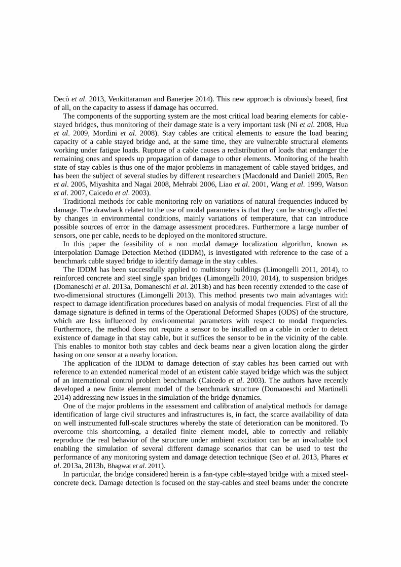
Fig. 7 Damage parameter and threshold: (a) B1; (b) B2; (c) B3; (d) B4; (e) B5

6.2 Damage in the deck steel beams supporting the concrete slab

Responses calculated with the finite element model have been also used to check the reliability

of the IDDM in locating the damaged portion of the bridge deck when the longitudinal steel beams

under the concrete slab are damaged.

The ODSs of the deck in the transversal and in the vertical directions of the bridge are the same

as reported in Fig. 5, limited to the frequency range 0-2 Hz. The ODSs have been obtained from

the Frequency Response Functions calculated from the responses at the nodes of the deck in the

transversal and in the vertical direction.

Also in these cases, the IDDM allowed both for detection and localization of the damage for all

the considered damage scenarios.

The values of the damage parameters ΔE(z), calculated on the base of the FRF recovered from

the transversal responses are reported in Figs. 7(a)-(e). As before, a blue vertical bar indicates the

actual location of damage (assumed at the node joining the two damaged elements) and the red

line represents the threshold corresponding to the 98% percentile of the damage parameter

distribution.

In all cases, for both single (B1, B4, B5) and multiple (B2, B3) damage scenarios the damaged

sections are correctly identified. Of course, as already discussed, the method is not able to indicate

if the damage is located in the beams, in the concrete slab or in the cables, since only responses

coming from the deck were considered in the procedure, but the damaged portion of the structure

has been correctly located.

The procedure shows a good accuracy and reliability being able to correctly locate damage

location in all the considered cases. Interestingly enough, different values of the damage index are

found at different locations for the same reduction of stiffness (compare Figs. 7(a), (d) for

example). This is likely depending on the different contributions of the modes that are more

influenced by damage at a given section. Future research work will be devoted to better investigate

these circumstances, in the hope of using of the proposed damage parameter to estimate also the

severity of damage at a given location.

7. Conclusions

The Interpolation Damage Detection Method was applied to detect damage in the supporting

system of a cable-stayed bridge object of an international benchmark problem. The damage

detection procedure used data that were derived form an extended numerical model of the Bill

Emerson Memorial cable stayed bridge. The finite element model herein considered extends the

benchmark one comprising new features such as soil structure interaction and deck-cables coupled

dynamics.

Results show that, if the Frequency Response Functions can be accurately estimated, the

proposed method is successful and reliable in detecting small and localized damages in the bridge

supporting system. This result can be accomplished using either the Frequency Response

Functions of the responses, calculated with respect to the base input, or using the Transmissibility

Functions calculated with respect to the response at a reference node. In the former case a higher

reliability of the results is obtained, also in the challenging case of multiple concomitant damaged

locations in the stay-cables supporting system. The last case is useful when the precise knowledge

of the input is not known.

When damage extends to the steel beams supporting the concrete slab, accurate results have

been also obtained for all the considered damage scenarios by employing the transversal response

of the deck, even when several damages coexist in different positions on the structure.

The main advantage of the IDDM method is the modest computational burden and the limited

user interaction it requires, that makes it very interesting for applications in the on-line monitoring

of structural systems, and particularly useful in the case of strategic structures and road

infrastructures expected to be self-diagnostic in order to exhibit efficient performances both for in

service conditions and in the aftermath of a catastrophic event.

References

ANSYS Rel. 14.0 (2014), Ansys Inc., Canonsburg PA, US.

Bhagwat, M., Sasmal, S., Novak, B. and Upadhyay, A. (2011), “Investigations on seismic response of two

span cable-stayed bridges”, Earthq. Struct., 2(4), 337-356.

Bocchini, P. and Frangopol, D. (2012), “Optimal resilience and cost-based post disaster intervention

prioritization for bridges along a highway segment”, J. Bridge Eng., ASCE, 17(1), 117-129.

Caicedo, J.M. and Dyke, S.J. (2005), “Experimental validation of structural health monitoring for flexible

bridge structures”, Sturct. Control Hlth. Monit., 12(3-4), 425-443.

Caicedo, J.M., Dyke, S.J., Moon, S.J., Bergman, L.A., Turan, G. and Hague, S. (2003), “Phase II benchmark

control problem for seismic response of cable-stayed bridges”, J. Struct. Control, 10(3-4), 137-168.

Decò, A., Bocchini, P. and Frangopol, D. (2013), “A probabilistic approach for the prediction of seismic

resilience of bridges”, Earthq. Eng. Struct. Dyn, 42(10), 1469-1487.

Dilena, M., Limongelli, M.P. and Morassi, A. (2015), “Damage localization in bridges via FRF interpolation

method”, Mech. Syst. Signal Pr., 52-53, 162-180.

Domaneschi, M. (2010), “Feasible control solutions of the ASCE benchmark cable-stayed bridge”, Struct.

Control Hlth. Monit., 17(6), 675-693.

Domaneschi, M. and Martinelli, L. (2012), “Performance comparison of passive control schemes for the

numerically improved ASCE cable-stayed bridge model”, Earthq. Struct., 3(2), 181-201.

Domaneschi, M. and Martinelli, L. (2014), “Extending the benchmark cable-stayed bridge for transverse

response under seismic loading”, J. Bridge Eng., 19(3), art. no. 4013003.

Domaneschi, M., Limongelli, M.P. and Martinelli, L. (2013a), “Vibration based damage localization using

MEMS on a suspension bridge model”, Smart Struct. Syst., 12(6), 679-694.

Domaneschi, M., Limongelli, M.P. and Martinelli, L. (2013b), “Multi-site damage localization in a

suspension bridge via aftershock monitorino”, Ingegneria Sismica, 30(3), 56-72.

Hua, X.G., Ni, Y.Q., Chen, Z.Q. and Ko, J.M. (2009), “Structural damage detection of cable-stayed bridges

using changes in cable forces and model updating”, Struct. Eng., ASCE, 135(9), 1093-1106.

Ismail, M., Rodellar, J., Carusone, G.., Domaneschi, M. and Martinelli, L. (2013), “Characterization,

modeling and assessment of Roll-N-Cage isolator using the cable-stayed bridge benchmark”, ACTA

Mech., 224(3), 525-547.

Liao, W.H., Wang, D.H. and Huang, S.L. (2001), “Wireless monitoring of cable tension of cable-stayed

bridges using PVDF Piezoelectric films”, J. Intell Mater. Syst. Struct., 12(5), 331-339.

Limongelli, M.P. (2003), “Optimal location of sensors for reconstruction of seismic responses through spline

function interpolation”, Earthq. Eng. Struct. Dyn., 32(7), 1055-1074.

Limongelli, M.P. (2010), “Frequency response function interpolation for damage detection under changing

environment”, Mech. Syst. Signal. Pr., doi:10.1016/j.ymssp.2010.03.004.

Limongelli, M.P. (2011), “The interpolation damage detection method for frames under seismic excitation”,

J. Sound Vib., 330(22), 5474-5489.

Limongelli, M.P. (2013), “Two dimensional damage localization using the interpolation method”, Key Eng.

Mater., 569, 860-867.

Macdonald, J.H.G. and Daniell, W.E. (2005), “Variation of modal parameters of a cable-stayed bridge

identified from ambient vibration measurements and FE modeling”, Eng. Struct., 27(13), 1916-1930.

Mehrabi, A.B. (2006), “In-service evaluation of cable-stayed bridges, overview of available methods, and

findings”, J. Bridge Eng., 11(6), 716-724.

Miyashita, T. and Nagai, M. (2008), “Vibration-based structural health monitoring for bridges using laser

doppler vibrometers and MEMS-based technologies”, Int. J. Steel Struct., 8(4), 325-331.

Mordini, A., Savov, K. and Wenzel, H. (2008), “Damage detection on stay cables using an open source-

based framework for finite element model updating”, Struct. Hlth. Monit., 7(2), 91-102.

Ni, Y.Q., Zhou, H.F., Chan, K.C. and Ko, J.M. (2008), “Modal flexibility analysis of cable-stayed Ting Kau

bridge for damage identification”, Comput. Aid. Civil Inf. Eng., 23(3), 223-236.

Phares, B., Lu, P., Wipf, T., Greimann, L. and Seo, J. (2013a), “Evolution of a bridge damage-detection

algorithm”, Trans. Res. Rec., 2331(1), 71-80.

Phares, B., Lu, P., Wipf, T., Greimann, L. and Seo, J. (2013b), “Field Validation of a Statistical-Based Bridge

Damage-Detection Algorithm”, J. Bridge Eng., 18(11), 1227-1238.

Ren, W.X., Peng, X.L. and Lin, Y.Q. (2005), “Experimental and analytical studies on dynamic characteristics

of a large span cable-stayed bridge”, Eng. Struct., 27(4), 535-548.

Ren, W.X., Lin, Y.Q. and Peng, X.L. (2007), “Field load tests and numerical analysis of Qingzhou cable-

stayed bridge”, J. Bridge Eng., 12(2), 261-270.

Seo, J., Phares, B., Lu, P., Wipf, T. and Dahlberg, J. (2013), “Bridge rating protocol using ambient trucks

through structural health monitoring system”, Eng. Struct., 46, 569-580.

Venkittaraman, A. and Banerjee, S. (2014), “Enhancing resilience of highway bridges through seismic

retrofit”, Earthq. Eng. Struct. Dyn., 43(8), 1173-1191.

Wang, D.H., Liu, J.S., Zhou, D.G. and Huang, S.L. (1999), “Using PVDF Piezoelectric Film sensors for In

Situ Measurement of stayed-cable tension of cable-stayed bridges”, Smart Mater. Struct., 8(5), 554-559.

Watson, C., Watson, T. and Coleman, R. (2007), “Structural monitoring of cable-stayed bridge: Analysis of

GPS versus modeled deflections”, J. Surv. Eng., 133(1), 23-28.