Peter Nyman

Representation ofQuantum Algorithmswith Symbolic Languageand Simulation onClassical Computer

Licentiate Thesis

Växjö University

School of Mathematics and System Engineering

Reports from MSI

Peter Nyman

Representation of Quantum Algorithmswith Symbolic Language and

Simulation on Classical Computer

Licentiate Thesis

Mathematic

Växjö University

A thesis for the Degree of Licentiate of Philosophy in Mathematic.

Representation of Quantum Algorithms with Symbolic Language andSimulation on Classical ComputerPeter Nyman

Växjö UniversitySchool of Mathematics and System EngineeringSE-351 95 Växjö, Swedenhttp://www.vxu.se/msi/

Reports from MSI, no 08092/2008ISSN 1650-2647ISRN VXU/MSI/MA/R/–08092–SE

To Carolina

AbstractQuantum computing is an extremely promising project combining theoreti-cal and experimental quantum physics, mathematics, quantum informationtheory and computer science. At the first stage of development of quantumcomputing the main attention was paid to creating a few algorithms whichmight have applications in the future, clarifying fundamental questions anddeveloping experimental technologies for toy quantum computers operatingwith a few quantum bits. At that time expectations of quick progress in thequantum computing project dominated in the quantum community. However,it seems that such high expectations were not totally justified. Numerousfundamental and technological problems such as the decoherence of quantumbits and the instability of quantum structures even with a small number ofregisters led to doubts about a quick development of really working quantumcomputers. Although it can not be denied that great progress had been madein quantum technologies, it is clear that there is still a huge gap between thecreation of toy quantum computers with 10-15 quantum registers and, e.g.,satisfying the technical conditions of the project of 100 quantum registers an-nounced a few years ago in the USA. It is also evident that difficulties increasenonlinearly with an increasing number of registers. Therefore the simulationof quantum computations on classical computers became an important partof the quantum computing project. Of course, it can not be expected thatquantum algorithms would help to solve NP problems for polynomial timeon classical computers. However, this is not at all the aim of classical simu-lation. Classical simulation of quantum computations will cover part of thegap between the theoretical mathematical formulation of quantum mecha-nics and the realization of quantum computers. One of the most importantproblems in “quantum computer science” is the development of new symboliclanguages for quantum computing and the adaptation of existing symboliclanguages for classical computing to quantum algorithms. The present the-sis is devoted to the adaptation of the Mathematica symbolic language toknown quantum algorithms and corresponding simulation on the classicalcomputer. Concretely we shall represent in the Mathematica symbolic lan-guage Simon’s algorithm, the Deutsch-Josza algorithm, Grover’s algorithm,Shor’s algorithm and quantum error-correcting codes. We shall see that thesame framework can be used for all these algorithms. This framework willcontain the characteristic property of the symbolic language representationof quantum computing and it will be a straightforward matter to include thisframework in future algorithms.

Key-words: Deutsch-Josza algorithm, Grover’s algorithm, Quantum com-puting, Quantum error-correcting, Shor’s algorithm, Simon’s algorithm, Si-mulation of quantum algorithms

v

SammanfattningUtvecklandet av kvantdatorn är ett ytterst lovande projekt som kombinerarteoretisk och experimental kvantfysik, matematik, teori om kvantinformationoch datalogi. Under första steget i utvecklandet av kvantdatorn låg huvudin-tresset på att skapa några algoritmer med framtida tillämpningar, klargöragrundläggande frågor och utveckla en experimentell teknologi för en leksaks-kvantdator som verkar på några kvantbitar. Då dominerade förväntningarnaom snabba framsteg bland kvantforskare. Men det verkar som om dessa sto-ra förväntningar inte har besannats helt. Många grundläggande och tekniskaproblem som dekoherens hos kvantbitarna och instabilitet i kvantstrukturenskapar redan vid ett litet antal register tvivel om en snabb utveckling avkvantdatorer som verkligen fungerar. Trots detta kan man inte förneka attstora framsteg gjorts inom kvantteknologin. Det råder givetvis ett stort gapmellan skapandet av en leksakskvantdator med 10-15 kvantregister och attt.ex. tillgodose de tekniska förutsättningarna för det projekt på 100 kvan-tregister som aviserades för några år sen i USA. Det är också uppenbartatt svårigheterna ökar ickelinjärt med ökningen av antalet register. Därför ärsimulering av kvantdatorer i klassiska datorer en viktig del av kvantdatorpro-jektet. Självklart kan man inte förvänta sig att en kvantalgoritm skall lösa ettNP-problem i polynomisk tid i en klassisk dator. Detta är heller inte syftetmed klassisk simulering. Den klassiska simuleringen av kvantdatorer kommeratt täcka en del av gapet mellan den teoretiskt matematiska formuleringen avkvantmekaniken och ett förverkligande av en kvantdator. Ett av de viktigasteproblemen i vetenskapen om kvantdatorn är att utveckla ett nytt symbolisktspråk för kvantdatorerna och att anpassa redan existerande symboliska språkför klassiska datorer till kvantalgoritmer. Denna avhandling ägnas åt en an-passning av det symboliska språket Mathematica till kända kvantalgoritmeroch motsvarande simulering i klassiska datorer. Konkret kommer vi att repre-sentera Simons algoritm, Deutsch-Joszas algoritm, Grovers algoritm, Shorsalgoritm och kvantfelrättande koder i det symboliska språket Mathematica.Vi använder samma stomme i alla dessa algoritmer. Denna stomme represen-terar de karaktäristiska egenskaperna i det symboliska språkets framställningav kvantdatorn och det är enkelt att inkludera denna stomme i framtidaalgoritmer.

Nyckelord: Deutsch-Josza algoritm, Grovers algoritm, Kvantdatorer, kvant-mekanisk felrättande kod, Shors algoritm, Simons algoritm, Simulering avkvantdatorer

vi

AcknowledgmentsI am grateful to my supervisor Professor Andrei Khrennikov for many di-scussions on the formulations of quantum mechanics and for the lessons inmathematics that he has given me.

I would like to thank Yaroslav Volovich who guided me into the researchfield, the simulation of quantum computers.

I am very thankful to Guillaume Adenier for all the discussions we havehad about the subject of quantum mechanics.

I am also thankful to my colleague in The School of Mathematics andSystems Engineering in Växjö University for their helpfulness and especiallythanks to Haidar Al-Talibi and Karoline Johansson.

I am grateful to all teachers for their lectures.Finally and foremost I would like to thank my family, Carolina, Adam

and Isak for their love and support.

vii

List of papers

I Simulation of Quantum Algorithms on a Symbolic Computer

II Simulation of Deutsch-Jozsa Algorithm in Mathematica

III Simulation of Simon’s Algorithm in Mathematica

IV A compact program code for simulations of quantum algorithms inclassical computers

V Simulation of Quantum Error Correcting Code

viii

Contents

Abstract v

Sammanfattning vi

Acknowledgments vii

List of papers viii

1 Introduction 11.1 Quantum Computing . . . . . . . . . . . . . . . . . . . . . . . 11.2 Simulation on classical computer . . . . . . . . . . . . . . . . 31.3 Simulation of Quantum Algorithms on a Symbolic Computer 51.4 Simulation of Deutsch-Jozsa Algorithm in Mathematica . . . 71.5 Simulation of Simon’s Algorithm in Mathematica . . . . . . . 81.6 A compact program code for simulations of quantum algo-

rithms in classical computers . . . . . . . . . . . . . . . . . . 81.7 Simulation of Quantum Error Correcting Code . . . . . . . . 9

2 Summary of papers 122.1 Simulation of Quantum Algorithms on a symbolic computer . 142.2 Simulation of Deutsch-Jozsa Algorithm in Mathematica . . . 242.3 Simulation of Simon’s Algorithm in Mathematica . . . . . . . 302.4 A compact program code for simulations of quantum algo-

rithms in classical computers . . . . . . . . . . . . . . . . . . 422.5 Simulation of Quantum Error Correcting Code . . . . . . . . 54

ix

Contents

x

Chapter 1

Introduction

1.1 Quantum Computing

In [1] Richard Feynman pointed out that it is totally impossible to efficientlysimulate quantum mechanics on classical computers.1 Consider a systemconsisting of N quantum particles. According to quantum formalism it isdescribed by the tensor product HN = H ⊗H ⊗ . . . ⊗H of the N copies ofthe state space H for a single particle. It is evident that the dimension ofHN grows exponentially with N. Feynman’s observation was the first steptoward the creation of quantum computers. Nowadays the main aim of thequantum computing project is not the simulation of quantum mechanicalstructures, but the execution of quantum algorithms for solving NP problemsin polynomial time.

Quantum computing is an extremely promising project combining theoret-ical and experimental quantum physics, mathematics, quantum informationtheory and computer science. The realization of this project provides theunique possibility for researchers working in various domains of science toexpand and check their theories and models. People working in quantumfoundations often consider quantum computers as a device to check such ba-sic principles of quantum mechanics as superposition and complementarityas well as the adequacy of the description of composite quantum systems bytensor products of Hilbert spaces, the unitarity of evolution in the absence ofmeasurement, the von Neumann projection postulate and Born’s rule. Sci-entists working in quantum information theory can finally approbate basicprinciples and constructions (the majority of which have been elaborated longbefore the quantum computing project) as well as develop mathematical mod-els, for example, for entanglement and decoherence. Experimenters proceedquickly by creating powerful sources of quantum bits, entangled particles andthe development of new quantum technologies.

At the first stage of the development of quantum computing the mainattention was paid to the creation of a few algorithms which may have appli-cations in the future, such as the clarification of foundational questions and

1Simulation is efficient if the execute time is in polynomial time

1

Chapter 1. Introduction

the development of experimental technologies for toy quantum computersoperating with a few quantum bits.

A number of quantum algorithms have been developed sinceDavid Deutschpresented the first algorithm [2]. This algorithm determines whether a Booleanfunction f : {0, 1} → {0, 1} is balanced or constant2. The Deutsch-Jozsa al-gorithm [3] is the generalization of Deutsch’s algorithm to a Boolean functionf : {0, 1}n → {0, 1}. The well-known classical algorithm should query thefunction more than 2n−1 + 1 times, while the quantum algorithm needs onlyone interaction with the oracle which implements the function.

Simon’s algorithm[4, 5] is similar to the Deutsch-Jozsa algorithm, but,instead of determining whether the Boolean function is balanced or constant,it is designed to find the period of a Boolean function f : {0, 1}n → {0, 1}n.A comparison with the well-known classical algorithm shows that the appli-cation of Simon’s algorithm [4, 5] (of course, on a quantum computer) wouldimply exponential speedup.

These first quantum algorithms have no direct practical applications.However, their creation played an important role in the quantum computingproject. It became evident that quantum computers might increase the speedof calculations tremendously.

Two algorithms with a greater potential for direct implementation to prac-tical application are Grover’s search algorithm [3] and Shor’s factorization al-gorithm [6]. Grover’s algorithm is a quantum search algorithm which searchesthrough an unsorted list with square roots less queries than the most effec-tive classical algorithm. Shor’s algorithm factorizes integers exponentiallyfaster than any of the classical algorithms. It has obvious applications tocryptography.

At the first stage of the quantum computing project expectations of quickprogress dominated in the quantum community. However, it seems thatsuch high expectations were not totally justified. Numerous foundationaland technological problems such as the decoherence of quantum bits and theinstability of quantum structures with an already sufficiently small numberof registers induced doubts about the quick elaboration of really workingquantum computers. Although it could not be denied that great progresshad been made in quantum technologies, it is clear that there is still a hugegap between the creation of toy quantum computers with 10-15 quantumregisters and satisfying e.g. the technical conditions of the project announceda few years ago in the USA: 100 quantum registers. It is also evident thatdifficulties increase nonlinearly with an increase in the number of registers.

Therefore the simulation of quantum computations on classical computersbecame an important part of the quantum computing project. Of course, one

2A Boolean function f : {0, 1}n → {0, 1} is constant if f(x) = 1 or f(x) = 0 for allinputs x and balanced if f(x) = 1 for half the inputs

2

1.2. Simulation on classical computer

could not expect that quantum algorithms would help to solve NP problemsfor polynomial time on classical computers. This is not at all the aim of clas-sical simulation, however. The classical simulation of quantum computationswill cover part of the gap between the theoretical mathematical formulationof quantum mechanics and the realization of quantum computers. One of themost important problems in “quantum computer scienc” is the developmentof new symbolic languages for quantum computing and the adaptation ofexisting symbolic languages to quantum algorithms.

The present thesis is devoted to the adaptation of the Mathematica sym-bolic language to known quantum algorithms and a corresponding simulationon a classical computer. Concretely we shall represent in the Mathematicasymbolic language Simon’s algorithm, Deutsch-Josza’s algorithm, Grover’salgorithm, Shor’s algorithm and quantum error-correcting codes.

We shall see that the same framework can be used for all these algorithms.This framework will express the characteristic property of the symbolic lan-guage representation of quantum computing. It will be a straightforwardmatter to include this framework in future algorithms.

1.2 Simulation on classical computer

Symbolic language for simulationIn this thesis it will be demonstrated that the Mathematica symbolic lan-guage can be used for all known quantum algorithms. This is a consequenceof the realization of all basis laws of quantum mechanics with the help ofMathematica: the superposition of quantum states, the representation of thestate of a composite system in the tensor product of Hilbert spaces describingthe states of the components of the system, Schödinger’s unitary evolutionand the measurement process based on von Neumann’s projection postulate.

Some blocks of the program code can be shared in all algorithms. Thesimulation procedure will adhere to the following pattern:

(a) definition (the framework),(b) the flow through the quantum circuit,(c) the measurement of a specially chosen observable on the output state.

Thus we start with the formalization in the Mathematica symbolic lan-guage of all basic elements of the mathematical formalism of quantum me-chanics which are used in quantum computing, e.g., qubits. Then we repre-sent the quantum circuits specific to the algorithm under investigation. Atthe end of the programming of the algorithm we need the symbolic languagerepresentation of the measurement.

Coming back to (a) we point out that in the symbolic language the repre-sentation corresponding to Dirac’s formalism with bra and ket vectors should

3

Chapter 1. Introduction

be constructed [7]. After this, superposition and tensor product, etc. are ex-pressed in symbolic Mathematica notations. Then, by moving to (b) weexpress quantum gates.

To be more precise, an arbitrary one-qubit quantum state

φ = c1 |0〉+ c2 |1〉

will be implemented asc1 e[0] + c2 e[1] ,

where e[j] , j = 0, 1, are symbolic Mathematica representations of the ba-sis vectors and cj , j = 0, 1 are complex numbers. An arbitrary one-qubitquantum operator is symbolized as

U :={ e[0] → c3 e[0] + c4 e[1] , e[1] → c5 e[0] + c6 e[1]}.

Thus:

U | (c1 e[0] + c2 e[1]) = (c1c3 + c2c5) e[0] + (c1c4 + c2c6) e[1]

Quantum CircuitIn the same way as classical algorithms are implemented on (classical) com-puters quantum circuits are implemented as schemes of quantum gates. Quan-tum gates are given by special unitary one- or two-qubit operators. In con-trast to classical gates, quantum gates are reversible.

In this thesis quantum circuits will be implemented in the symbolic lan-guage and then they will be used for simulation on the basis of the schemewhich is standard for quantum computing – a combination of a few quantumgates. A quantum circuit can be presented as

|0〉U

FE |0〉 U

UFE

|0〉 U FE Figure 1. Quantum circuit

where U is some one- or two-qubit gate. This quantum circuit will be imple-mented in the simulation as

U2,3|(U1,2|(U3|(U2| e[0, 0, 0]))),

where the index of U indicates to which of the qubits the gate is applied.

4

1.3. Simulation of Quantum Algorithms on a Symbolic Computer

HistoryRichard Feynman [1] proposed to make simulations of quantum mechanics ona quantum computer, which is essentially different (even from the viewpointof computer science) from the classical Turing machine. David Deutsch [3]developed the idea of quantum computing and introduced a quantum me-chanical analogue of the Turing machine. He also found a proper problemfor quantum computing, which he solved by the quantum algorithm. Hence,Deutsch showed a prospect for the development of quantum computers. Afew new algorithms were created after Deutsch.

However, one should be well aware about the following problem in quan-tum computing.3 Unfortunately, the number of known quantum algorithmsand problems which can be solved is not so large. Moreover, it seems thatthe last few years were not signified by the creation of new interesting quan-tum algorithms. It might be that this situation in quantum computing isnot occasional (so one might not simply say: "we need more time to createnew quantum algorithms"). One could not exclude that there are some deeproots behind the insufficient algorithmic structure of quantum computing.Such roots may be created by computer science and the general theory ofalgorithms.

This is why it is so important to simulate quantum computing by usingdifferent classical languages (such as C [8], Maple [9], Mathematica [10], etc)and also by developing specific languages for quantum simulations such as[11, 12], etc. Some of the programming languages used for simulations ofquantum computers were conceived as programming languages for quantumcomputers and not only for simulations.

Of course, people performing simulations of quantum computing by us-ing different symbolic languages as well as developing special languages forquantum programming dream about developing new quantum algorithms byclarifying the logic and algorithmic structure.

1.3 Simulation of Quantum Algorithms on aSymbolic Computer

This thesis consists of four papers in the field of simulation of quantum algo-rithms on classical computers by using the Mathematica symbolic languageand one paper about simulation of error correcting code. In the first paper“Simulation of Quantum Algorithms on a symbolic compute” we introduce

3Here quantum computing is considered from the point of view of computer scienceand not really from the view of quantum physics. Thus we are not interested so much inphysical processes which take place in quantum computers and the problems related tothese processes, e.g. decoherence.

5

Chapter 1. Introduction

the basic framework and implement Shor’s algorithm in this symbolic simu-lation. Simulation with the Mathematica symbolic language consists of twoparts: the first part defines the characteristic property of the symbolic lan-guage and the second part implements the quantum algorithms and simulatesmeasurement.

The part devoted to symbolic representation describes the quantum gatesand quantum registers. In fact, one can consider this part as the symboliclanguage representation of notions of quantum mechanics used in quantumcomputers: superposition, tensor product, entanglement and operators. Bythis symbolic formalization we prepare a classical computer for operationswith quantum gates and states. A sequence of quantum gates generates aquantum circuit and consequently implements a quantum algorithm. Thecapability of these simulations is shown by the implementation of Shor’salgorithm, which is a well-known quantum factorization algorithm with futureapplications in cryptography. The realization of Shor’s algorithm on quantumcomputers would provide a new possibility to destroy the safety of public-keycryptos.

Before introducing the quantum Fourier transform, which plays a basicrole in Shor’s algorithm, let us consider one simple example of quantumcircuit represented in the symbolic language. In general, one qubit state isrepresented in the symbolic language as

e[ψ] = α e[0] + β e[1] ,

where α and β are complex numbers in the way that the sum of squares oftheir absolute values is equal to one. Here e[0] and e[1] are representations ofDirac’s notations in Mathematica. Generalization to the case of multi-qubitsis evident. Let us regard the definitions part as executed and then apply thisto a state e[00] in the following quantum gate.

Consider the Pauli operator X = |1〉 〈0|+ |0〉 〈1| and the Hadamard oper-ator H = 1/

√2(|0〉 〈0|+ |1〉 〈0|+ |0〉 〈1| − |1〉 〈1|) and the quantum circuit

e[0]H⊗2 FE

e[0] X FE ↑ ↑ ↑ ↑

e[ψ0] e[ψ1] e[ψ2] e[ψ3]

Let the initial state be e[00] . We apply X2, H1 and H2 to the first and secondqubit. Thus the new state will be

H1|H2|X2| e[00] = 1/2 ( e[00]− e[01] + e[10]− e[11])

where we leaving out the parentheses.

6

1.4. Simulation of Deutsch-Jozsa Algorithm in Mathematica

This is straightforward in simulation in Mathematica;

In[10] := H1| (H2| (X2| e[0, 0]))

The result is given by

out[10] :=12e[0, 0] +

12e[0, 1]− 1

2e[1, 0]− 1

2e[1, 1]

Shor’s algorithm contains a part of classical algorithm and the quantumFourier transform (QFT). The QFT is a quantum analogous to the classi-cal discrete Fourier transform. QFT contains the following quantum gates:Hadamard operator H, Controlled Not operator and Rotation operator R.The implementation of QFT will follow from the QFT Circuit:

|j1〉 H R2 · · · Rn−1 Rn · · · · · ·

|j2〉 • · · · H R2 · · · Rn−1 · · ·...

. . . · · · . . . · · · · · ·|jn−1〉 · · · • · · · · · · H R2

|jn〉 · · · • · · · • · · · • H

where we omit the Controlled Not gates which swap the order of the qubitsat the end of the circuit. This circuit is directly implemented by the code

H1|R1,2| · · · |R1,n−1|R1,n|H2|R2,3| · · · |R2,n−1| · · · |Hn−1|Rn−1,n−2|Hn| e[ψ]

in this simulation language (leaving out the parentheses).

1.4 Simulation of Deutsch-Jozsa Algorithm inMathematica

This paper represents Deutsch-Jozsa’s algorithm in the Mathematica simu-lation language. Deutsch-Jozsa’s algorithm was the first quantum algorithm.This simple algorithm demonstrated the opportunity of quantum comput-ing. The commission for this algorithm is easy: we need to decide whether aBoolean function is balanced or constant. Our aim is to make a simulationof this quantum algorithm in the symbolic language. The definition sectioncontains one gate and a so-called quantum oracle. A quantum oracle is anoperator in a black box defined as:

Uf |x〉⊗n|y〉 = |x〉⊗n|y ⊕ f(x)〉

Let us give a simplified picture of this task. Bob selects a balanced or con-stant Boolean function and Alice’s task is to determine function property.

7

Chapter 1. Introduction

Alice uses a quantum computer to implement the algorithm by means of thequantum circuit:

|0〉⊗n / HUf

H FE |1〉 H

.

Alice prepares the initial state e[0, 0, 0, . . . , 1] and the quantum gate accord-ing to the scheme in the circuit

Hn−1| . . .H2|H1|Uf |Hn| . . .H2|H1| e[0, 0, 0, . . . , 1] .

Finally, the measurement is performed.She should apply the oracle once, instead of using the classical algorithm

and query the function at least 2n−1 + 1 times.

1.5 Simulation of Simon’s Algorithm in Math-ematica

The simulation of Simon’s algorithm is performed in the third paper. Thestructure of this algorithm is similar to that of Deutsch-Jozsa’s algorithm. Italso contains an oracle. The essential difference is the function given by theoracle. Bob selects a periodic function and Alice’s task is to find the period.Alice prepares the state e[0, 0, . . .] , applies the quantum gates and the oracleand finally, Alice performs the measurement. She continues by restartingthe algorithm until she obtains a sufficient number of values to solve a linearequation giving the answer.

1.6 A compact program code for simulations ofquantum algorithms in classical computers

Grover’s algorithm is a search algorithm for unsorted lists. This quantumalgorithm needs a O(

√N) query as an alternative to O(N) for the classical

algorithm, where N is the number of elements in the list. Moreover, thisalgorithm uses an oracle and, in fact, repeats the query of the oracle (Groveriteration) until the probability to obtain the searched element approachesmax.

We prepare the initial state e[0, 0, 0, . . . , 1] , and then apply the Hadamardgate to all qubits. After this, we repeat the Grover iteration and perform themeasurement. This flow for Grover’s algorithm is given by the following

8

1.7. Simulation of Quantum Error Correcting Code

circuit:Grover iteration︷ ︸︸ ︷

|0〉⊗q /H⊗q+1 Uf

H⊗q

U0

H⊗q FE |1〉

↑ ↑ ↑ ↑ ↑ ↑ ↑e[ψ0] e[ψ1] e[ψ2] e[ψ3] e[ψ4] e[ψ5] e[ψ6]

_ _ _ _ _ _ _ _ _ _ _ _ _����

����

_ _ _ _ _ _ _ _ _ _ _ _ _

Grover’s algorithm circuit using one Grover iteration

1.7 Simulation of Quantum Error CorrectingCode

This study considers implementations of error correction in a simulation lan-guage on a classical computer. Error correction will be necessary in quantumcomputing and quantum information. We will implement Shor code as anexample of error corrections code. The Shor code is a development of the clas-sical error correcting code known as majority voting. There are some greatdifferences between quantum and classical error correcting. Measurementsdestroy the quantum states and another problem in quantum computing iscontinuous errors. Moreover, it is impossible to clone an arbitrary quantumstate. In classical computing will errors imply that bits flips, but continuouserrors in the quantum computing imply that the states phases flips or thatthe qubits flips or some combination of this errors. Shor code will overcomethese problems in quantum computing.

9

Bibliography

[1] R.P. Feynman. Simulating Physics with Computers. International Jour-nal of Theoretical Physics, 21:467, 1982.

[2] D. Deutsch. Quantum theory, the Church-Turing principle and theuniversal quantum computer. Proceedings of the Royal Society ofLondon. Series A, Mathematical and Physical Sciences (1934-1990),400(1818):97–117, 1985.

[3] D. Deutsch and R. Jozsa. Rapid solution of problems by quantum com-putation. Proc Roy Soc Lond A, 439:553–558, October 1992.

[4] D.R. Simon. On the power of quantum computation. In Proceedings ofthe 35th Annual Symposium on Foundations of Computer Science, pages116–123, Los Alamitos, CA, 1994. Institute of Electrical and ElectronicEngineers Computer Society Press.

[5] D.R. Simon. On the power of quantum computation. SIAM J. Comput.,26(5):1474–1483, 1997.

[6] P.W. Shor. Polynomial-time algorithms for prime factorization and dis-crete logarithms on a quantum computer. SIAM Journal on Computing,26(5):1484–1509, 1997.

[7] P.A.M. Dirac. The Principles of Quantum Mechanics. Clarendon Press,1995.

[8] B. Ömer. Structured Quantum Programming. PhD thesis, Ph. D. Thesis,Technical University of Vienna, 2003.

[9] T. Radtke and S. Fritzsche. Simulation of n-qubit quantum systems. IV.Parametrizations of quantum states, matrices and probability distribu-tions. Computer Physics Communications, 2008.

[10] J.M. Burdis B .Juliá-Díaz and F. Tabakin. Qdensity-a mathematicaquantum computer simulation. Computer Physics Communications,174:914–934, 2006.

[11] JW Sanders and P. Zuliani. Quantum Programming, Mathematics ofProgram Construction. Springer-Verlag LNCS, 1837:80–99, 2000.

10

Bibliography

[12] S. BETTELLI, T. CALARCO, and L. SERAFINI. Toward an archi-tecture for quantum programming. The European physical journal. D,Atomic, molecular and optical physics, 25(2):181–200, 2003.

11

Chapter 2

Summary of papers

I Simulation of Quantum Algorithms on a Symbolic Computer

II Simulation of Deutsch-Jozsa Algorithm in Mathematica

III Simulation of Simon’s Algorithm in Mathematica

IV A compact program code for simulations of quantum algorithms inclassical computers

V Simulation of Quantum Error Correcting Code

13

Paper I

2.1 Simulation of Quantum Algorithms on asymbolic computer

15

Simulation of Quantum Algorithms on asymbolic computer

Peter Nyman

International Center for Mathematical Modelingin Physics, Engineering and Cognitive science

MSI, Växjö University, S-35195, Sweden

Abstract. This paper is a presentation of how to implement quantum algorithms (namely, Shor’salgorithm ) on a classical computer by using the well-known Mathematica package. It will giveus a lucid connection between mathematical formulation of quantum mechanics and computationalmethods.

Keywords: Shor’s factoring algorithm, prime factorization, quantum computing, Mathematica,quantum Fourier transformPACS: 03.67.Lx, 02.70.-c, 07.05.Tp

INTRODUCTION

A couple of examples of various methods for the simulation of quantum algorithmswere given in [1, 2]. In preprint [3] we introduced a computational language constructedon the basis of quantum mechanics. We have decided to implement the well-knownShor’s factoring algorithm as an example of a quantum algorithm. The aim is to con-struct a computational language in order to present a straightforward connection betweenDirac’s mathematical formulation of quantum mechanics and the program code. Thus,the computational language will include quantum mechanical terminology such as quan-tum operators and quantum states.

THE SIMULATION FRAMEWORK

A quantum state in n dimensions can be represented by a linear combination of nnumbers of basis vectors. In the two-dimensional case a quantum state |φ〉 is representedas a superposition of two basis vectors, say |0〉 and |1〉, (computation basis [4, 5]). Inthis case a quantum state |φ〉 is represented as

|φ〉 = α|0〉+β |1〉, (1)

where α and β are complex numbers having the sum of squares equal one.We will introduce new symbols for states of this computational basis as follows:

e[0] = |0〉 and e[1] = |1〉. This is the foundation for the structure of the program code.For more than one-qubit we will use the computational basis states e[x1, . . . ,xn] =|x1 . . .xn〉, where x j ∈ {0,1} or by using the more compact notation e[y] = |y〉, wherey = xn20 + · · ·+x12n−1. We will, write the state φ as e[φ ] = αe[0]+βe[1], by analogy to

equation (1). The operator A acting on the state φ is often written as A|φ〉 in the quantummechanical literature. To match these symbols, we will use the computational symbolsA|e[φ ] for this operation. The program code must be able to handle the linearity of tensorproduct. Let e[v],e[w] be vectors and α a scalar. We define the tensor product as

α(e[v]⊗ e[w]) = (αe[v])⊗ e[w] = e[v]⊗ (αe[w]) (2)(e[v1]+ e[v2])⊗ e[w] = e[v1]⊗ e[w]+ e[v2]⊗ e[w] (3)

e[v]⊗ (e[w1]+ e[w2]) = e[v]⊗ e[w1]+ e[v]⊗ e[w2]. (4)

We add two commands to the program code that will implement this definition ofthe tensor product. The command e[a__ ,α_ .e[x__ ],b__ ] := αe[a,x,b] will transform(αe[v])⊗e[w] and e[v]⊗ (αe[w]) to ξ α(e[v]⊗e[w]). The next command e[a,ξ (α e[x]+β e[y]),b] := ξ αe[a,x,b]+ξ βe[a,y,b] will transform e[v1]⊗ξ (α e[w1]+β e[w2])⊗e[v1]to ξ α(e[v1]⊗ e[w1]⊗e[v2])+ξ β (e[v1]⊗ e[w2]⊗e[v2]). Let U be an arbitrary one-qubitquantum gate. Then U will transform an arbitrary state e[φ ] which is represented in thecomputational basis states as e[φ ] = ae[0] + be[1] to the state U |e[φ ] → a(c1 e[0] +c2 e[1])+ b(c3 e[0] + c4 e[1]), where a,b,ci ∈ C. Now we add a Mathematica gate U tothe program code resulting in U |e[0] → c1 e[0] + c2 e[1] and U |e[1] → c3 e[0] + c4 e[1].For example, the Hadamard gate H will be added in Mathematica as the commandH:={e[0]→ 1/

√2(e[0]+ e[1]), e[1]→ 1/

√2(e[0]− e[1])}. We will define a one-qubit

gate Oi as an operator which acts on the qubit in position i and leaves the other qubitsunchanged. The program code must be able to operate with a gate on arbitrary qubit.Consequently we will define an operator Oi in the Mathematica code. The operator willbe defined Oi = I⊗i−1 ⊗U ⊗ I⊗n−i as an operator which acts on n-qubits,where I is theone-qubit unit operator and U is an arbitrary one-qubit operator. Then operator Oi is afunction of Oi|e[v] → e[ψ]. Similarly, we will define Oi, j as an operator which operatesas the two-qubits operator on the qubits in positions i, j and leaves the other qubitsunchanged. Now we have the tools to build quantum circuits. To achieve this, we willuse a quantum Fourier transform circuit in Shor’s factoring algorithm.

AN INTRODUCTION TO SHOR’S FACTORING ALGORITHM

Prime factorizing of an odd number N can be accomplished using Shor’s algorithm [6].If N is an even integer then we divide it with 2 n-times until 2−nN becomes an oddnumber. An even N = 2n can easily be found in view of the fact that 2n ≡ 0 (mod 2).Let N be the composite of prime factors so that

N = pα11 pα2

2 . . . pαkk , (5)

where k > 1 and αi ∈ Z+. The algorithm will be able to factorize the integer N. Wecan also assume that N is not a prime power, i.e. k > 1 and that there exists at least onepi �= p j. A prime power can be found with a known classical method in polynomial time.Let us choose a x ∈ ZN randomly, where ZN = {1,2, . . . ,N −1,N}. The next step is touse Euclid’s algorithm which determines the greatest common divisor. If x and N are notrelatively prime, then we will find a factor by using Euclid’s algorithm. A factor is equal

to gcd(x,N) if gcd(x,N) �= 1. If x and N are relatively prime, the task will be to find theorder of x in the group ZN . The algorithm will search for the smallest r ∈ Z+ so thatxr ≡ 1 (mod N); consequently r is called order r of x. If

xr ≡ 1 (mod N) (6)

and r is a even integer, then it is possible to factorize xr −1 as

xr −1 = (xr2 −1)(x

r2 +1). (7)

The integer N will share at least one factor with (xr2 − 1) or (x

r2 + 1) since N divides

xr − 1. These factors can calculate be with Euclid’s algorithm. Let us presume that aneven r has been found, which gives us the possibility to determine the factors equalto gcd(x

r2 + 1,N) and gcd(x

r2 − 1,N). There is nevertheless an obvious exclusion that

xr2 ≡ 1 (mod N) due to the definition of order r. However, it may occur that x

r2 ≡ −1

(mod N), i.e. only trivial factors will be found since N is the greatest common divisor tox

r2 +1 and N. There will be two factors, gcd(x

r2 +1,N) and gcd(x

r2 −1,N), in case the

order r of x is an even number and xr2 �≡ −1 (mod N).

THE QUANTUM FOURIER TRANSFORM

The discrete Fourier transform maps a vector V1 = α0,α1, . . . ,αn−1 to another vectorV2 = β0,β1, . . .βk . . . ,βn−1, where α,β ∈ C. In traditional mathematics the discreteFourier transform is defined as follow:

V2 =1√n

n−1

∑j=0

α je2πi jk/n. (8)

The quantum Fourier transform (QFT) is similar to the discrete Fourier transform, yetQFT will be represented in computational symbols. The QFT is a function which actson q = log2 n qubits.

Definition 1. The quantum Fourier transform is a function which maps basis states to alinear combination of basis states

QFT |e[ j] =1√n

n−1

∑k=0

e2πi jk/n e[k]. (9)

The quantum Fourier transform for a arbitrary state ψ is

QFT |n−1

∑j=0

α j e[ j] =1√n

n−1

∑k=0

αke2πi jk/n e[k]. (10)

The decomposable of QFT is used to match quantum gates.

Lemma 1.

QFT |e[ j] =1√n(e[0]+ e

2π i j21 e[1])⊗ (e[0]+ e

2π i j22 e[1])⊗·· ·⊗ (e[0]+ e

2π i jn e[1]). (11)

We will construct this decomposition by using the Rotation, the Hadamard and theCNOT gates. Every arbitrary unitary operator may be represented by combinations ofsingle qubit gates and CNOT gates [5]. QFT can be expressed in single quantum gatesas:

Swap(Hq(Rq,q−1Hq−1(· · ·(Rq,2 · · ·R3,2H2(Rq,1 · · ·R2,1H1|e[u]))))), (12)

where swap is a combination of 3q numbers of CNOT gates. This decomposition of QFTrequires q operations on the first qubit and q−1 operations on the second qubit, and soon. Hence it follows that the decomposition needs 1

2(q + 1)q H and Rk operations. Toobtain the right order, we swap the decomposition; thus we need 3q/2 or 3(q− 1)/2more operations. Altogether, the decomposition of QFT is require in the order of q2

gates e.i. QFT uses O(q2) elementary operations.

QUANTUM COMPUTATION AND SHOR’S FACTORINGALGORITHM.

Shor’s algorithm can be executed in four steps. First let us choose an arbitrary integerx ∈ Z

+ which will be smaller than the integer N that we want to factorize. The secondstep is to make sure that the chosen integer is not a prime factor. If it is a prime factorthe algorithm can result in the prime factor and stop the algorithm. It is only in the thirdstep we need to implement the algorithms in a quantum computer. At this stage we willuse the quantum Fourier transform in the algorithm to find the order r of x. Restart thealgorithm if r is odd or x

r2 ≡ −1 (mod N). In the last stage a classical computer will

calculate the factors and output gcd(xr2 ±1,N). Let us start the algorithm with an N and

choose n = 2q so that N2 ≤ n ≤ 2N2. It will prepare two registers e[0]e[0] with q- qubitsin the quantum computer.

1. Let us set up the first register in superposition

1√n

n−1

∑c=0

e[c]e[0]. (13)

2. Let us then compute xc (mod N) in the second register and the computer will be instate

1√n

n−1

∑c=0

e[c]e[xc modN]. (14)

3. Next, we need to compute the QFT on the first register e[c]

QFT |e[c] =1√n

n−1

∑k=0

e2πick/n e[k]. (15)

The machine will be in state

ψ =1n

n−1

∑c=0

n−1

∑k=0

e2πick/n e[k]e[xc modN]. (16)

Now let us measure the first register in the quantum machine for any k in e[k]. Order r ofx can be found as a denominator of one of the convergents to k/n, where the probabilityto find r depends on the number of qubits. To find the order r, we need to apply continuedfractions to the k/n

SHOR’S ALGORITHM IN THE MATHEMATICA CODE

This chapter will introduce a Mathematica program code which implements Shor’s algo-rithm in a classical computer. We will follow the Mathematica program code evolutionsand compare this with Shor’s algorithm. This comparison will demonstrate a connectionbetween the classical computer and the quantum computer. The program will try to findtwo factors to N, where N is an odd prime factorization and has at least two differentprime factors.

� � 3�5; q � �Log�2, �2��;Do�x � Random�Integer, �2, � � 1��;If�GCD�x, �� �� 1, SecondStep; QFT; OutPrint

, Print�"Chosen x�", x, " a multiplier of " , GCD�x, ���, ".";�;, �

160�Log�Log�����������������������������������������������

9

��������

The algorithm will choose q=⌈Log2(N2)

⌉so that the algorithm will find a factor with

large probability, i.e. if it selects q to satisfy N2 ≤ 2q < 2N2, the two factors will thenbe found with a probability of at least 9

160log logN . The program will choose a randominteger x ∈ {2,3, · · · ,N −1}.

�� NumberTheory`ContinuedFractions`

e�a___, Α_.�e�x__�, b___� :� Α e�a, x, b�e�a___, Ξ_.��Α_.�e�x__� � Β_.�e�y__��, b___� :� Ξ Α e�a, x, b� � Ξ Β e�a, y, b�O_ i_ � v_ :� Chop�Expand�v �. �e�x__� ReplacePart�e�x�, e��x��i�� �. O, i����O_ i_,j_ � v_ :� Chop�Expand�v �. �e�x__�

�e��x��i�, �x��j��j�i �. O �. e�Α_, Β_� e�Sequence �� Take��x�, i � 1�,Α,

Sequence �� Take��x�, �i � 1, j � 1��,Β,

Sequence �� Take��x�, �j � 1, �1�������H :� e�0�

1���������������2

��e�0� � e�1��, e�1� 1

���������������2

��e�0� � e�1���

R :� e�1, 1�d_ ���������2d �e�1, 1��

Swap :� e�i_, j_�_ e�j, i��

We will only use the computational basis states e[x1, . . . ,xn], where x j ∈ {0,1}.The commands e[a__ ,α_ .e[x__ ],b__ ] := αe[a,x,b] and e[a,ξ (α e[x] + β e[y]),b] :=ξ αe[a,x,b]+ξ βe[a,y,b] will give the program code a connection to the tensor product.The command O_ i_|v_ is a one-qubit operator which takes vector v as an attributeand operates with O on the qubit in position i. Likewise, the command O_ i_ , j_|v_ is a

two-qubits operator which takes vector v as an input and operates with O on the qubitin position i and j. To compute QFT the algorithm requires three gates, Hadamard (H),Rotation (R) and Swap (Swap).

FirstStep�q_, x_, �_� :� Expand� 1���������������������2q

� �c�0

2q�1

e�Sequence �� IntegerDigits�c, 2, q�, Sequence �� IntegerDigits�0, 2, q��

SecondStep :��������Secstep�q_, x_, �_� :� Expand� 1

���������������������2q

� �c�0

2q�1

e�Sequence �� IntegerDigits�c, 2, q�,

Sequence �� IntegerDigits�Mod�xc, ��, 2, q�� ; u � Secstep�q, x, ���������

The command FirstStep prepares the first register in a superposition. Since the first stepis pointless in a classical computer; consequently it will be excluded in the code and wego directly to the second step in the code. Secstep calculates xc (mod N) in the secondregister, where q is the number of qubits.

QFT :� �For�i � 1, i � q, i��, u � Hi � u; For�j � i � 1, j � q, j��, u � Ri,j � u��;For�i � 1, i � IntegerPart� q

����2

, i��, u � Swapi,q�1�i � u ;OutQFT � �u ��. a_.�e�y___� � b_.�e�y___� Together��a � b���e�y��;Probability � List �� OutQFT �. Α_.�e�y___� � �Abs�Α�2., e�y��;Probability � Probability �. �a_, e�y__�� � a;

b � �Probability�1��;For�i � 2, i � Length�Probability�, i��, b � AppendTo�b, b�i � 1� � Probability�i���;r � Random��;For�i � 1, i � Length�b�, i��, If�r � b��i��, MeasureQFTStep � i; Break����;p � �List �� OutQFT �. _.�e�x__� FromDigits��Sequence �� Take��x�, q��, 2���

The QFT will act on the state u by means of the three gates in the following order:Hq(Rq,q−1Hq−1(· · ·(Rq,2 · · ·R3,2H2(Rq,1 · · ·R2,1H1 e[u])))). The third line in the programcode will swap the qubits. All terms with identical computational basis states will becollected in the command OutQFT. Probability is a list of the probabilities used tomeasure one of the terms in the register. One of the terms will be randomly chosen takinginto consideration of probability to measure the state. The position of the chosen termwill be saved in MeasureQFTStep. Finally, the list p of decimal numbers is derivedfrom the binary list OutQFT.

OutPrint :� ����CFD :� Denominator�Convergents� p�MeasureQFTStep�

�������������������������������������������������2q

;

Do�If�Mod�xCFD�i�, �� � 1 && EvenQ�CFD�i�� && Mod�x CFD�i����������������2 , � � � � 1,

Print�"Factors a1�", GCD��, xCFD�i����������������

2 � 1 , " and", " a2�",

GCD��, xCFD�i����������������

2 � 1 , " have been found." ; �, �i, 1, Length�CFD�� ;����

The randomly chosen value in the register is in p[[MeasureQFTStep]]. In CFD theprogram saves the denominator of convergents p[[MeasureQFTStep]]/2q. From this

we can select all even denominators, where xCFD ≡ 1 (mod N) and xCFD

2 �= N − 1(mod N). If any of the denominators satisfies these three conditions, it will give us twofactors.

CONCLUSION

In this study we have constructed a computational language for simulations of quantumalgorithms and presented the program code for an algorithm. We have also demonstratedthat every unitary operator has a representation in this computational language. Animportant future challenge is to develop this computational language to include thetheory of density operator.

ACKNOWLEDGMENTS

I would like to thank my supervisor Prof. Andrei Khrennikov for fruitful discussions onthe foundations of quantum computing. I am also grateful to Yaroslav Volovich for hisinvolvement and ideas in this research.

REFERENCES

1. B.Juliá-Díaz, J.M. Burdis and F. Tabakin, “QDENSITY-A Mathematica Quantum Computer simula-tion”, Com. Phys. Com., Vol.175, 914-934, (2006).

2. T Altenkirch and J Grattage, “A functional quantum programming language”, In Proceedings of the20th Annual IEEE Symposium on Logic in Computer Science, IEEE Computer Society, (2004).

3. P. Nyman “Quantum Computing - Declarative computational methods for simulation of quantumalgorithms and quantum errors”, Research report Växjö University, Sweden, (2005),http://www.vxu.se/msi/forskn/exarb/2005/05153.pdf

4. M. Hirvensalo, Quantum Computing, Springer-Verlag, Berlin, Heidelberg, 2001.5. M. Nielsen and I. Chuang, Quantum Computing and Quantum Information, Cambridge University

Press, 2000.6. P.W. Shor, “Introduction to Quantum Algorithms” , Florham Park, USA, (2001),

http://xxx.lanl.gov/abs/quant-ph/0005003

Paper II

2.2 Simulation of Deutsch-Jozsa Algorithm inMathematica

25

Simulation of Deutsch-Jozsa Algorithm in Mathematica

Peter Nyman

International Center for Mathematical Modelingin Physics, Engineering and Cognitive science

MSI, Växjö University, S-35195, Sweden

Abstract. This study examines the simulation of Deutsch-Jozsa algorithm in Mathematica. The program code implementedon a classical computer will be a straight connection between the mathematical formulation of quantum mechanics andcomputational methods in Mathematica. This program code will be a foundation of a universal simulation language.

Keywords: Deutsch-Jozsa algorithm, quantum computing, MathematicaPACS: 03.67.Lx, 02.70.-c, 07.05.Tp

INTRODUCTION

A general quantum simulation language on a classical computer will open the opportunity to compare an experientialresult from the developments of quantum computers with the mathematical theory. Our aim is therefore to construct ageneral program code where it will be easy to implement algorithms. A couple of examples of various methods for thesimulation of quantum algorithms were given in [1, 2, 3]. We have in previous research [4] studied Shor’s algorithm[5] and implemented this algorithm in the high-level language Mathematica. A simulation of a quantum algorithm onclassical computers will give us the possibility to comparethe results of quantum computers with the output of thephysically more stable classical computers. In the development of quantum algorithms it will be interesting to test newalgorithms on a classical computer. This article will describe the connection between future quantum computers andtoday’s simulations of quantum computers. Thus, the computational language will include the quantum mechanicalterminology such as quantum operators and quantum states. This simulation language will include the most essentialoperations in quantum computing. Examples of these operations will be theHadamard, Controlled notandToffoligates. In earlier studies (see [6]) we have introduced a framework in a computational language constructed on theformulation of quantum mechanics. In this study we will go further and use this framework when we implementDeutsch-Jozsa algorithmas an example of a quantum algorithm. The aim is to construct acomputational languageand describe a straightforward connection betweenDirac’s mathematical formulation of quantum mechanics and ourprogram code. However, the mathematically described algorithms will have a clear mathematical structure even afterthat we have implemented this algorithms as a program code. Moreover a program with mathematical structure willgive us short program codes and this simulation of Deutsch-Jozsa algorithm will use only few lines of program code.This simulation is a link from the mathematical theory of quantum algorithms to its implementation on a quantumcomputer. Let us begin with a demonstration of the frameworkwe have constructed in the high-level program languageMathematica, this will probably be used for future algorithms.

THE SIMULATION FRAMEWORK

This section we will introduce a framework constructed for the simulation of quantum algorithms on classicalcomputers. We will point out that there is a symbolic similarity between our framework and the mathematicalframework. This framework will be a computational dual toDirac’s bra-ket notation. A quantum state inn dimensionscan be represented by a linear combination ofn numbers of basis vectors. In the two-dimensional case a quantum state|φ〉 is represented as a superposition of two basis vectors ,say|0〉 and|1〉, known as computational basis (computationalbasis, see [7, 8]). In this basis a quantum state|φ〉 is represented as

|φ〉 = α|0〉+β |1〉, (1)

whereα andβ are complex numbers such as|α|2 + |β |2 = 1. We will introduce some new symbols for the statesof the computational basis as follows: e[0] = |0〉 and e[1] = |1〉. This is the foundation for the structure of theprogram code. For more than one-qubit we will use the computational basis states e[x1, . . . ,xn] = |x1 . . .xn〉, wherex j ∈ {0,1} or by using the more compact notation e[y] = |y〉, wherey = xn20 + · · ·+ x12n−1. We will, write the stateφ as e[φ ] = αe[0] + βe[1], by analogy to (1). The operatorA acts on the stateφ and is often written asA|φ〉 inthe quantum mechanical literature. To match these symbols,we will use the computational symbolsA|e[φ ] for thisoperation. A computational problem will be that the computer must regard expressions equal if they have identicalmeaning even if these notations are not identical. As an example the expression e[0,e[1],1] must be equal to e[0,1,1]in the code. We can bring in the command e[0,e[1],1] := e[0,1,1] or the more general e[a__,e[b__],c__] := e[a,b,c]to solve this problem. Moreover, the program code must be able to handle the linearity of the tensor product. Let e[ . ]be vectors andα a complex number. We define the tensor product as

α(e[v]⊗e[w]) = (αe[v])⊗e[w] = e[v]⊗ (αe[w]) (2)

(e[v1]+e[v2])⊗e[w] = e[v1]⊗e[w]+e[v2]⊗e[w] (3)

e[v]⊗ (e[w1]+e[w2]) = e[v]⊗e[w1]+e[v]⊗e[w2]. (4)

We add two commands to the program code that will implement this definition of the tensor product. The command

e[a___, α_. e[x__], b___] := α e[a, x, b]

will transform e[a]⊗αe[x]⊗e[c] to αe[a⊗x⊗b] = αe[a,x,b]. This command is the computational dual to the tensorexpression in Dirac’s notation|a〉⊗α|x〉⊗ |b〉 = α|axb〉. The other command

e[a___, ξ_. (α_. e[x__] + β_. e[y__]), b___]:=ξ αe[a, x, b]+ ξ βe[a, y, b]

will transform e[a]⊗ ξ (α e[x] + β e[y])⊗e[b] to ξ αe[a,x,b] + ξ βe[a,y,b]. Let U be an arbitrary one-qubit quantumgate. ThenU will transform an arbitrary state e[φ ] which is represented in the computational basis states as e[φ ] =ae[0]+be[1] to the stateU |e[φ ] → a(c1e[0]+c2e[1])+b(c3e[0]+c4e[1]), wherea,b,ci are complex numbers. Weadd theMathematicagateU to the program code as followsU |e[0]→ c1e[0]+c2e[1] andU |e[1]→ c3e[0]+c4e[1]. Forexample, the Hadamard gateH will be added in Mathematica as the commandH:={e[0]→ 1/

√2(e[0]+ e[1]), e[1]→

1/√

2(e[0]− e[1])}. We will define a one-qubit gateOi as an operator which acts on the qubit in positioni and leavesthe other qubits unchanged. The program code must be able to operate with a gate on an arbitrary qubit. Consequentlywe will define an operatorOi in the Mathematica code. Defined the operatorOi asOi = I⊗i−1⊗U ⊗ I⊗n−i which actson n-qubits, whereI is the one-qubit unit operator andU is an arbitrary one-qubit operator. Then operatorOi is afunction ofOi |e[v] → e[ψ]. Similarly, we will defineOi, j as an operator which operates as the two-qubits operator onthe qubits in positionsi, j and leaves the other qubits unchanged. Now we have the tools to build quantum circuits.

AN INTRODUCTION TO THE DEUTSCH-JOZSA ALGORITHM

The function f : {0,1}n → {0,1} is constant if all output is 0 or 1 for all input. The functionf is balanced if halfof all outputs are 0. The Deutsch-Jozsa problem was introduced by David Deutsch and Richard Jozsa with the taskto decide the functionf property, which will be constant or balanced (see [9]). The most naive classical algorithmwill need 2n−1 + 1 outputs to decide the property of the function. Deutsch andJozsa showed that the Deutsch-Jozsaalgorithm would solve this task with only one output. In the implementation of Deutsch-Jozsa algorithm we will useto the unitary operator Uf which we defined as

Uf : |x〉⊗n|y〉 = |x〉⊗n|y⊕ f (x)〉

where⊕ is the binary addition modulo 2. We will use the function Uf:= e[i__, j_ ] :→ e[i,Mod[j + f[i],2]] to apply thisoperator in our simulation language. Let us describe Deutsch-Jozsa problem in the following example, Bob choose afunction with one of the two properties, constant or balanced, and Alice task is to decide its property. To her delightshe will get Bob to calculate this function in a quantum computer. Bob prepare the register in superposition before heoperates with the operator Uf that will act on all qubits at once. Before Bob measure the register and send the result toAlice he will apply the Hadamard gate to then−1 first qubits. If Bob sends|0〉⊗n to Alice then she will be sure thathis function was constant, otherwise she will make a conclusion that the function was balanced.

|0〉⊗n / HU f

HFE

|1〉 H

Figure 1. The Deutsch-Jozsa algorithm circuit

THE DEUTSCH-JOZSA ALGORITHM IN A SYMBOLIC LANGUAGE

Let us use our simulation language to help Alice solve her problem to decide the functions property. You may followthe algorithm in the circuit in figure 1. We start on the left with the register e[0, · · · ,0,1] and operate Hadamard gateH:={e[0] → 1/

√2(e[0]+ e[1]), e[1] → 1/

√2(e[0]− e[1])} on this state which will place all qubits in superposition

ψ1 =1√2n+1 ∑

x∈{0,1}ne[x](e[0]− e[1]).

At this point we will use the operator Uf and the register willbe in the stateψ2

ψ2 =1√2n+1 ∑

x∈{0,1}n(−1) f (x) e[x](e[0]− e[1]).

Before measurement the algorithm will apply the Hadamard operation on all qubits except the last one and

ψ3 =1

2n+1/2 ∑z∈{0,1}n

∑x∈{0,1}n

(−1)x·z+ f (x) e[z](e[0]− e[1]),

wherex ·z= x1z1 +x2z2 + · · ·+xnzn mod 2. Measurement of the firstn will give the output e[0, · · · ,0] if and only iff is constant, otherwise it is balanced. This will follow fromthe fact that the probability to measure e[0, · · · ,0] is

12n

∣∣ ∑

x∈{0,1}n(−1)x·0+ f (x)∣∣2 (5)

and it will be one if f (x) = 0 or f (x) = 1 for all x where0 = {0,0, . . . ,0}. Moreover, it will be zero probability tomeasure e[0, · · · ,0] if f is balanced since (5) will be equal to zero.

THE DEUTSCH-JOZSA ALGORITHM IN MATHEMATICA

The Deutsch-Jozsa algorithm is implemented as follow. We will begin to define characteristic properties of quantumcomputers in the program code.

Listing 1: Definition of register and quantum gates in mathematica.

e[a___, α_. e[x__], b___] := α e[a, x, b]

e[a___, ξ_. (α_. e[x__] + β_. e[y__]), b___]:=ξ αe[a, x, b]+ ξ βe[a, y, b]

O_i_ |v_:= Chop[Expand[v /. (e[x__] :→ ReplacePart[e[x], e[{x}[[i]]] /. O,i])]]

O_i_ j_ |v_:= Chop[Expand[v /. O]]

H := {e[0] :→ 1/√

2 (e[0] + e[1]),e[1] :→ 1/√

2 (e[0] - e[1])}

Uf := {e[i___, j_] :→ e[i, Mod[j + f[i], 2]]}

Enlarge[ψ_,i_] := ψ /. ψ -> (ψ /.e[x_]:→ e[Sequence@@Table[0, {i - 1}], x])

The essential points of this framework is linearity and the tensor products. We have described before how tensor prod-ucts and a register will be represented in our simulation language. The two-first lines (see listing 1) are computationallypowerful and they will manage to implement some of the essential properties in simulation as linearity, superposition

and tensor products. Line 3-4 in the same listing will define the operator mapping one or two qubits respectively. TheDeutsch- Jozsa algorithm only need to apply the two operators H andU f . The last line will enlarge a state of theone qubit e[1] to then-qubit state e[0,0,0, . . . ,1]. The operators, linearity, superposition and tensor products are nowdefined. The implementation of the algorithm will follow from the listing 2.

Listing 2: Deutsch-Jozsa algorithm in mathematica.

q = 8;

φ = Enlarge[e[1],q];

Do[φ = (Hi | φ), {i,q}];

φ = Ufq−1,q | φ;φ = φ /. {f[1, x__]:→0,f[0, x__]:→1};

Do[φ = (Hi | φ), {i,q - 1}];

φ

There are certain advantages to compare this listing 2 with the circuit (1). By using the commandEnlarge on statee[1], defined in line 2, will the register will be prepared in theq-qubit state e[0,0,0, . . . ,1]. In listing 2 on line 3-4 theHadamard operator and the unitary function are applied on all the qubits in the register. In line 5 we will be able tochoose the function property. In this example we have chosena balanced function. The algorithm will output the resultwhen the Hadamard operator have been applied on theq−1 first qubits. The output will contain zeros inq−1 firstqubits if and only if f is constant, otherwise it is balanced.

CONCLUSION

In this study we have constructed a computational language for simulations of quantum algorithms and presented aprogram code for Deutsch-Jozsa algorithm. We have also demonstrated a general framework for simulation of quantumcomputers on classical computers. An important future challenge is to develop this computational language to includethe most of the well-known quantum algorithms.

ACKNOWLEDGMENTS

I would like to thank my supervisor Prof. Andrei Khrennikov for fruitful discussions on the foundations of quantumcomputing. I am also grateful to Yaroslav Volovich for his involvement and ideas in this research.

REFERENCES

1. J.M. Burdis B .Juliá-Díaz and F. Tabakin. Qdensity-a mathematica quantum computer simulation.Computer PhysicsCommunications, 174:914–934, 2006.

2. P. Dumai H. Touchette. Qucalc - the quantum computation package formathematica. http://crypto.cs.mcgill.ca/QuCalc/,October 2007.

3. L. Spector.Automatic Quantum Computer Programming: A Genetic Programming Approach. Springer, 2004.4. P. Nyman. Simulation of quantum algorithms with a symbolic programming language.ArXiv e-prints, 705, may 2007.5. P.W. Shor. Polynomial-time algorithms for prime factorization and discrete logarithms on a quantum computer.SIAM Journal

on Computing, 26(5):1484–1509, 1997.6. P. Nyman. Quantum computing - declarative computational methods for simulation of quantum algorithms and quantum errors.

Master’s thesis, Växjö University, Sweden, 2005.7. M.A. Nielsen and I.L. Chuang.Quantum Computation and Quantum Information. Cambridge University Press, October 2000.8. M.Hirvensalo.Quantum Computing. Springer Series on Natural Computing. Springer, 1st edition edition, 2001.9. D. Deutsch and R. Jozsa. Rapid solution of problems by quantum computation. Proc Roy Soc Lond A, 439:553–558, October

1992.

Paper III

2.3 Simulation of Simon’s Algorithm inMathematica

31

Simulation of Simon’s Algorithm inMathematica

Peter NymanInternational Center for Mathematical Modeling in Physics,Engineering and Cognitive science, MSI ,Vaxjo University,

S-35195, Sweden

AbstractA general quantum simulation language on a classical computer

provides the opportunity to compare an experiential result from thedevelopment of quantum computers with mathematical theory. Theintention of this research is to develop a program language that is ableto make simulations of quantum mechanical processes as well as quan-tum algorithms. This study examines the simulation of quantum algo-rithms on a classical computer with a symbolic programming language.We use the language Mathematica to make a simulation of well-knownquantum algorithms. The program code implemented on a classicalcomputer will be a straight connection between the mathematical for-mulation of quantum mechanics and computational methods. Thisgive us an uncomplicated and clear language for implementations ofalgorithms. The computational language includes essential formula-tions such as quantum state, superposition and quantum operator.This symbolic programming language provides a universal frameworkfor examining the existing as well as future quantum algorithms. Thisstudy contributes with an implementation of a quantum algorithm ina program code where the substance is applicable in other simulationof quantum algorithms.

keywords:Mathematica, Simon’s Algorithm, Quantum AlgorithmSimulation, Quantum Computing

1 Introduction

Our aim is to construct a general program code where it will be easy toimplement algorithms. A couple of examples of various methods for the sim-

1

ulation of quantum algorithms were given in the papers [1, 2, 3, 4]. We havein previous research [5] studied Shor’s algorithm [6] and implemented thisalgorithm in the high-level language Mathematica. A simulation of a quan-tum algorithm on classical computers will give us the possibility to comparethe results of quantum computers with the output of the physically morestable classical computers. In the development of quantum algorithms itwill be interesting to test new algorithms on a classical computer. This ar-ticle will describe the connection between future quantum computers andtoday’s simulations of quantum computers. Thus, the computational lan-guage will include the quantum mechanical terminology such as quantumoperators and quantum states. This simulation language will include themost essential operations in quantum computing. Examples of these oper-ations will be the Hadamard, Controlled not and Toffoli gates. In earlierstudies (see [7]) we have introduced a framework in a computational lan-guage constructed on the formulation of quantum mechanics. In this studywe will go further and use this framework when we implement Simon’s al-gorithm as an example of a quantum algorithm. The aim is to construct acomputational language and describe a straightforward connection betweenDirac’s mathematical formulation of quantum mechanics and our programcode. However, the mathematically described algorithms will have a clearmathematical structure even after that we have implemented this algorithmsas a program code. Moreover a program with mathematical structure willgive us short program codes and this simulation of Simon’s algorithm willuse only few lines of program code. This simulation is a link from the math-ematical theory of quantum algorithms to its implementation on a quantumcomputer. Let us begin with a demonstration of the framework we have con-structed in the high-level program language Mathematica, this will probablybe used for future algorithms.

2 The Simulation Framework

This section we will introduce a framework constructed for the simulation ofquantum algorithms on classical computers. We will point out that there is asymbolic similarity between our framework and the mathematical framework.This framework will be a computational dual to Dirac’s bra-ket notation. Aquantum state in n dimensions can be represented by a linear combinationof n numbers of basis vectors. In the two-dimensional case a quantum state|φ〉 is represented as a superposition of two basis vectors ,say |0〉 and |1〉,known as computational basis (computational basis, see [8, 9]). In this basis

2

a quantum state |φ〉 is represented as

|φ〉 = α|0〉+ β|1〉, (1)

where α and β are complex numbers such as |α|2+|β|2 = 1. We will introducesome new symbols for the states of the computational basis as follows: e[0] =|0〉 and e[1] = |1〉. This is the foundation for the structure of the programcode. For more than one-qubit we will use the computational basis statese[x1, . . . , xn] = |x1 . . . xn〉, where xj ∈ {0, 1} or by using the more compactnotation e[y] = |y〉, where y = xn20 + · · ·+x12

n−1. We will, write the state φas e[φ] = αe[0] + βe[1], by analogy to (1). The operator A acts on the stateφ and is often written as A|φ〉 in the quantum mechanical literature. Tomatch these symbols, we will use the computational symbols A|e[φ] for thisoperation. A computational problem will be that the computer must regardexpressions equal if they have identical meaning even if these notations arenot identical. As an example the expression e[0, e[1], 1] must be equal toe[0, 1, 1] in the code. We can bring in the command e[0, e[1], 1] := e[0, 1, 1] orthe more general e[a , e[b ], c ] := e[a, b, c] to solve this problem. Moreover,the program code must be able to handle the linearity of the tensor product.Let e[ . ] be vectors and α a complex number. We define the tensor productas

α(e[v]⊗ e[w]) = (αe[v])⊗ e[w] = e[v]⊗ (αe[w]) (2)

(e[v1] + e[v2])⊗ e[w] = e[v1]⊗ e[w] + e[v2]⊗ e[w] (3)

e[v]⊗ (e[w1] + e[w2]) = e[v]⊗ e[w1] + e[v]⊗ e[w2]. (4)

We add two commands to the program code that will implement this defini-tion of the tensor product. The command

e[a___,α_.e[x__],b___]:=αe[a,x,b]

will transform e[a]⊗αe[x]⊗ e[c] to αe[a⊗x⊗ b] = αe[a, x, b]. This commandis the computational dual to the tensor expression in Dirac’s notation |a〉 ⊗α|x〉 ⊗ |b〉 = α|a x b〉. The other command

e[a___,ξ_.(α_.e[x__]+β_.e[y__]),b___]:=ξαe[a,x,b]+ξβe[a,y,b]

will transform e[a]⊗ξ(α e[x]+β e[y])⊗e[b] to ξαe[a, x, b]+ξβe[a, y, b]. Let Ube an arbitrary one-qubit quantum gate. Then U will transform an arbitrarystate e[φ] which is represented in the computational basis states as e[φ] =a e[0] + b e[1] to the state U | e[φ] → a(c1 e[0] + c2 e[1]) + b(c3 e[0] + c4 e[1]),where a, b, ci are complex numbers. We add the Mathematica gate U to theprogram code as follows U | e[0] → c1 e[0]+c2 e[1] and U | e[1] → c3 e[0]+c4 e[1].For example, the Hadamard gate H will be added in Mathematica as the

3

command H:={ e[0] → 1/√

2( e[0] + e[1]), e[1] → 1/√

2( e[0] − e[1])}. Wewill define a one-qubit gate Oi as an operator which acts on the qubit inposition i and leaves the other qubits unchanged. The program code mustbe able to operate with a gate on an arbitrary qubit. Consequently we willdefine an operator Oi in the Mathematica code. Defined the operator Oi asOi = I⊗i−1 ⊗ U ⊗ I⊗n−i which acts on n-qubits, where I is the one-qubitunit operator and U is an arbitrary one-qubit operator. Then operator Oi

is a function of Oi| e[v] → e[ψ]. Similarly, we will define Oi,j as an operatorwhich operates as the two-qubits operator on the qubits in positions i, j andleaves the other qubits unchanged. Now we have the tools to build quantumcircuits.

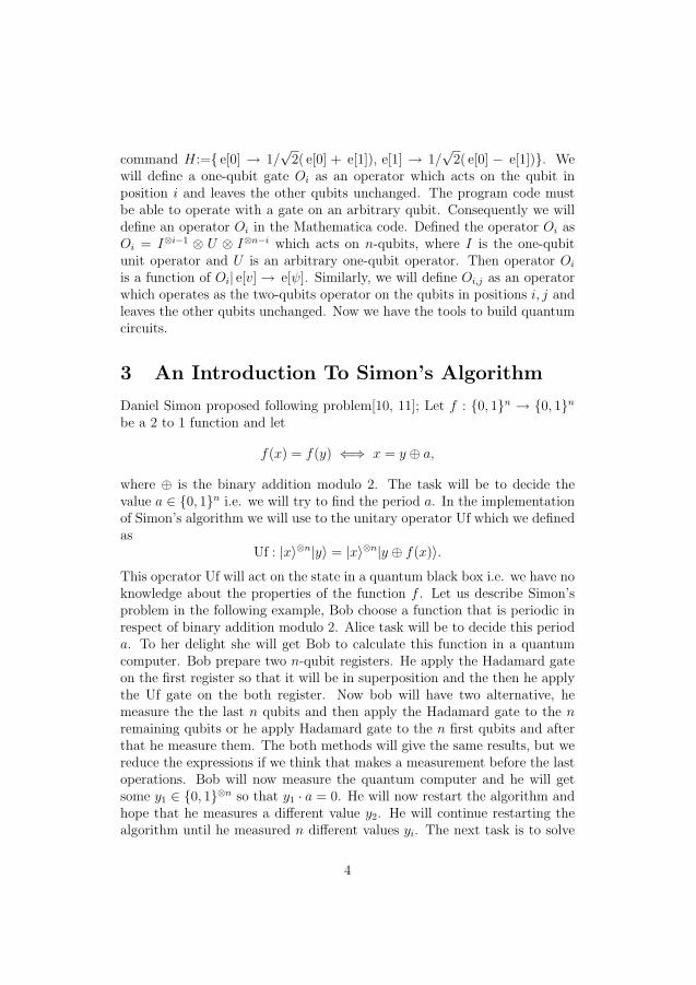
3 An Introduction To Simon’s Algorithm

Daniel Simon proposed following problem[10, 11]; Let f : {0, 1}n → {0, 1}n

be a 2 to 1 function and let

f(x) = f(y) ⇐⇒ x = y ⊕ a,

where ⊕ is the binary addition modulo 2. The task will be to decide thevalue a ∈ {0, 1}n i.e. we will try to find the period a. In the implementationof Simon’s algorithm we will use to the unitary operator Uf which we definedas

Uf : |x〉⊗n|y〉 = |x〉⊗n|y ⊕ f(x)〉.

This operator Uf will act on the state in a quantum black box i.e. we have noknowledge about the properties of the function f . Let us describe Simon’sproblem in the following example, Bob choose a function that is periodic inrespect of binary addition modulo 2. Alice task will be to decide this perioda. To her delight she will get Bob to calculate this function in a quantumcomputer. Bob prepare two n-qubit registers. He apply the Hadamard gateon the first register so that it will be in superposition and the then he applythe Uf gate on the both register. Now bob will have two alternative, hemeasure the the last n qubits and then apply the Hadamard gate to the nremaining qubits or he apply Hadamard gate to the n first qubits and afterthat he measure them. The both methods will give the same results, but wereduce the expressions if we think that makes a measurement before the lastoperations. Bob will now measure the quantum computer and he will getsome y1 ∈ {0, 1}⊗n so that y1 · a = 0. He will now restart the algorithm andhope that he measures a different value y2. He will continue restarting thealgorithm until he measured n different values yi. The next task is to solve

4

a linear equation so that yi · a = 0 for all i ∈ {1, 2, . . . , n}

|0〉⊗n / HUf

H NM

|0〉⊗n / H NM

Figure 1. The Simon’s algorithm circuit

4 The Simon’s Algorithm in a Symbolic Lan-

guage

Let us use our simulation language to decide the period a of a periodic func-tion i.e. we search for a a so that f(x) = f(y) ⇐⇒ x = y ⊕ a. Prepare tworegisters with the states e[0]⊗n and then begin with the algorithm, with canbe followed in figure 1. The first operations will be to act with the Hadamardgate on the first register. The registers will now be in superposition of thestates e[x] e[0]⊗n so that

ψ1 =1√2n

∑x∈{0,1}⊗n

e[x] e[0]⊗n.

In this step the Uf operator act on the both registers and then the registerswill be in the states;

ψ2 =1√2n

∑x∈{0,1}⊗n

e[x] e[f(x)].

Measure the second register for some state f(x0) where x0 ∈ {0, 1}⊗n. Allthe state f(x) will have equal probability 2−n to be measured. Moreover,since f(x0) = f(x0 + a) are the first register in the states

ψ3 =1√2

( e[x0] + e[x0 ⊕ a]) ,

after measurement of the second register. Then apply Hadamard to ψ3 anduse that H e[x] =

∑y(−1)x·y e[y] to get

ψ4 =1√2n+1

∑y∈{0,1}⊗n

((−1)x0·y + (−1)(x0⊕a)·y) e[y]

or equivalent

ψ4 =1√2n−1

∑y:y·a=0

(−1)x0·y e[y].

5

Measurement of the first register will give a y0 ∈ {0, 1}⊗n where y0 · a = 0.Now restart the algorithm and measure a new value y1 with the probability1−2/2(n−1) that satisfy y1 6= y0 and y1 6= 0, in that case this gives a equationy1 · a = 0 where y1 linearly independent to y0. We will repeat this to weobtain n − 1 numbers of linearly independent equations y0 · a = 0, y1 · a =0, . . . , y(n−2) · a = 0 to solve. In generality will the probability be 1− 21+i−n

for i < n to measure a yi so that y0 · a = 0, y1 · a = 0, . . . , y(i−1) · a = 0 islinearly independent. Solve the equations to find a.

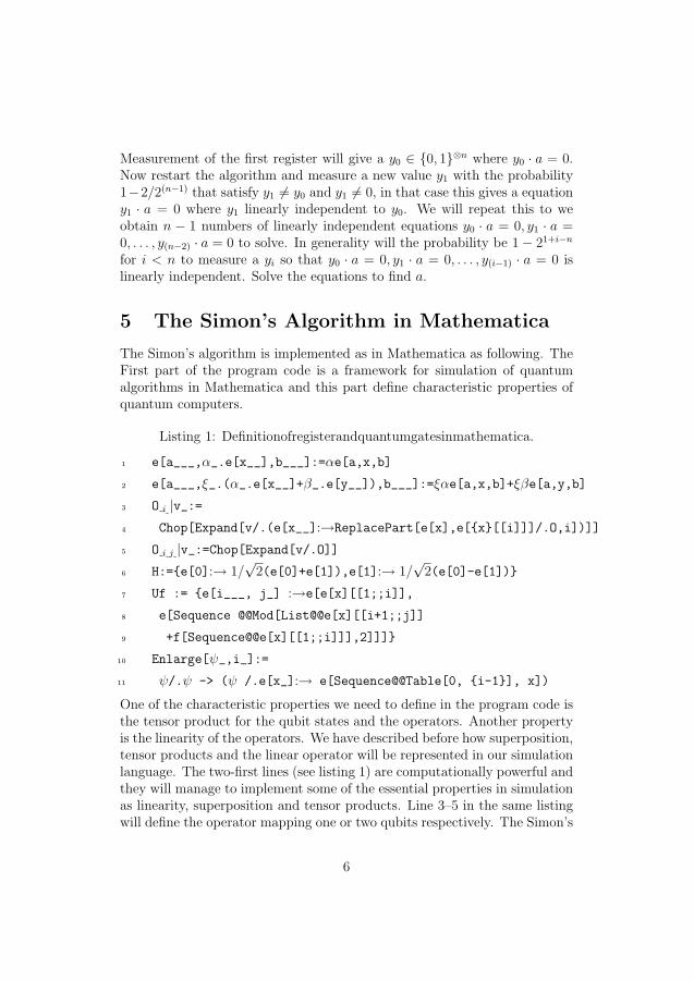
5 The Simon’s Algorithm in Mathematica

The Simon’s algorithm is implemented as in Mathematica as following. TheFirst part of the program code is a framework for simulation of quantumalgorithms in Mathematica and this part define characteristic properties ofquantum computers.

Listing 1: Definitionofregisterandquantumgatesinmathematica.

1 e[a___,α_.e[x__],b___]:=αe[a,x,b]

2 e[a___,ξ_.(α_.e[x__]+β_.e[y__]),b___]:=ξαe[a,x,b]+ξβe[a,y,b]

3 O i |v_:=4 Chop[Expand[v/.(e[x__]:→ReplacePart[e[x],e[{x}[[i]]]/.O,i])]]

5 O i j |v_:=Chop[Expand[v/.O]]6 H:={e[0]:→ 1/

√2(e[0]+e[1]),e[1]:→ 1/

√2(e[0]-e[1])}

7 Uf := {e[i___, j_] :→e[e[x][[1;;i]],

8 e[Sequence @@Mod[List@@e[x][[i+1;;j]]

9 +f[Sequence@@e[x][[1;;i]]],2]]]}

10 Enlarge[ψ_,i_]:=

11 ψ/.ψ -> (ψ /.e[x_]:→ e[Sequence@@Table[0, {i-1}], x])

One of the characteristic properties we need to define in the program code isthe tensor product for the qubit states and the operators. Another propertyis the linearity of the operators. We have described before how superposition,tensor products and the linear operator will be represented in our simulationlanguage. The two-first lines (see listing 1) are computationally powerful andthey will manage to implement some of the essential properties in simulationas linearity, superposition and tensor products. Line 3–5 in the same listingwill define the operator mapping one or two qubits respectively. The Simon’s

6

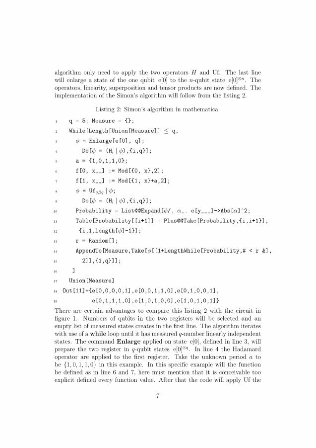
algorithm only need to apply the two operators H and Uf. The last linewill enlarge a state of the one qubit e[0] to the n-qubit state e[0]⊗n. Theoperators, linearity, superposition and tensor products are now defined. Theimplementation of the Simon’s algorithm will follow from the listing 2.

Listing 2: Simon’s algorithm in mathematica.

1 q = 5; Measure = {};

2 While[Length[Union[Measure]] ≤ q,

3 φ = Enlarge[e[0], q];

4 Do[φ = (Hi | φ),{i,q}];5 a = {1,0,1,1,0};

6 f[0, x__] := Mod[{0, x},2];

7 f[1, x__] := Mod[{1, x}+a,2];

8 φ = Ufq,2q | φ;9 Do[φ = (Hi | φ),{i,q}];

10 Probability = List@@Expand[φ/. α_. e[y___]->Abs[α]^2;

11 Table[Probability[[i+1]] = Plus@@Take[Probability,{i,i+1}],

12 {i,1,Length[φ]-1}];

13 r = Random[];

14 AppendTo[Measure,Take[φ[[1+LengthWhile[Probability,# < r &],

15 2]],{1,q}]];

16 ]

17 Union[Measure]

18 Out[11]={e[0,0,0,0,1],e[0,0,1,1,0],e[0,1,0,0,1],

19 e[0,1,1,1,0],e[1,0,1,0,0],e[1,0,1,0,1]}

There are certain advantages to compare this listing 2 with the circuit infigure 1. Numbers of qubits in the two registers will be selected and anempty list of measured states creates in the first line. The algorithm iterateswith use of a while loop until it has measured q-number linearly independentstates. The command Enlarge applied on state e[0], defined in line 3, willprepare the two register in q-qubit states e[0]⊗q. In line 4 the Hadamardoperator are applied to the first register. Take the unknown period a tobe {1, 0, 1, 1, 0} in this example. In this specific example will the functionbe defined as in line 6 and 7, here must mention that it is conceivable tooexplicit defined every function value. After that the code will apply Uf the

7

both registers where the first register is the control qubits and the second istargets qubits. Then apply the Hadamard gate to the first register beforemeasurement. Moreover will a measurement of the first register means thatone state of all the q-qubit states in superposition will be randomly chosenwhere the measurement probability is equal to square of the absolute value ofthe phase. Consequently, must the simulation of a measurement depend onthe phase. As a first step to make a measurement will line 10 to 12 create alist called Propability, with contains the probability to measure the states.The algorithm chose a randomly r ∈ [0, 1]. This random r decides whichof the element (state) that will be measured in the list Propability. Thewhile loop in the final line will measure an element and add it to the listMeasure. Finally the latest line will output all measured elements in thelist Measure. It remains to solve the linear equation to find a, but since itwill be done in a classical computer will we leave this besides. We can easyverify that y · a = 0 for all measured states in the output.

6 Results

The program have been tested for a number different periods that require2 to 6 qubits registers (see table 1 for the result of some of the test). Theruntime for 6 qubit registers indicates to be around 300 second. The resultfrom the test with more than 6 qubits showed that this simulation of Simon’salgorithm will give a long runtime larger registers.

7 conclusion

We have constructed a computational language for simulations of quantumalgorithms with are presented by implementation of Simon’s algorithm. Thisdemonstrates a part of a general framework for simulation of quantum com-puters on classical computers. The test shows that this simulation is noteffective for registers with more than 6 qubits. An important future chal-lenge is to continue to develop this computational language to include allwell-known quantum algorithms.

8

Period Output Runtime/second

{0, 0, 1} {e[0,0,0],e[0,1,0],e[1,0,0],e[1,1,0]} 0.125{0, 1, 0} {e[0,0,0],e[0,0,1],e[1,0,0],e[1,0,1]} 0.157{1, 1, 1} {e[0,0,0],e[1,0,1],e[1,1,0],e[1,0,1]} 0.187{0, 1, 1, 0} {e[0,0,0,0],e[0,0,0,1],e[1,0,0,0],e[1,0,0,1],e[0,1,1,0]} 0.375{0, 0, 1, 0} {e[0,0,0,0],e[0,0,0,1],e[1,0,0,0],e[1,0,0,1],e[1,1,0,1]} 0.437{1, 0, 1, 0} {e[0,0,0,0],e[0,0,0,1],e[0,1,0,1],e[1,0,1,0],e[1,1,1,1]} 0.313{0, 1, 1, 0, 0} {e[0,0,0,1,1],e[0,1,1,0,1],e[1,0,0,1,0],e[1,1,1,0,0],

e[1,1,1,0,1],e[1,1,1,1,0]} 5.203{1, 0, 1, 1, 0} {e[0,0,0,0,1],e[0,1,0,0,1],e[0,1,1,1,1],e[1,0,0,1,0],

e[1,0,1,0,0],e[1,1,1,0,1]} 7.344{1, 1, 1, 0, 0} {e[0,1,1,0,0],e[0,1,1,0,1],e[0,1,1,1,0],e[1,0,1,0,1],

e[1,0,1,1,0],e[1,1,0,0,0]} 3.157{1, 0, 1, 1, 0, 0} {e[0,0,0,0,0,1],e[0,0,0,0,1,1],e[0,0,1,1,1,0],e[1,0,0,1,1,0],

e[1,1,0,1,0,0],e[1,1,1,0,0,1],e[1,1,1,0,1,0]} 215.265{1, 1, 1, 1, 0, 0} {e[0,0,0,0,1,1],e[0,0,1,1,0,1],e[0,1,0,1,1,0],e[0,1,1,0,1,1],

e[1,1,0,0,0,1],e[1,1,1,1,0,0],e[1,1,1,1,0,1]} 306.938

Table 1: Test results

8 acknowledgments

I would like to thank my supervisor Professor Andrei Khrennikov for fruitfuldiscussions on the foundations of quantum computing. I am also gratefulto Yaroslav Volovich for his involvement and ideas in the beginning of thisresearch.

References

[1] J. B. B .Julia-Dıaz and F. Tabakin, “Qdensity-a mathematica quan-tum computer simulation,” Computer Physics Communications 174,pp. 914–934, 2006.

[2] P. D. H. Touchette, “Qucalc-the quantum computation package formathematica.” http://crypto.cs.mcgill.ca/QuCalc/, October 2007.

[3] L. Spector, Automatic Quantum Computer Programming: A GeneticProgramming Approach, Springer, 2004.

9

[4] S. Aaronson and D. Gottesman, “Improved simulation of stabilizer cir-cuits,” Physical Review A (Atomic, Molecular, and Optical Physics)70(5), p. 052328, 2004.

[5] P. Nyman, “Simulation of quantum algorithms with a symbolic pro-gramming language,” ArXiv e-prints 705, may 2007.

[6] P. Shor, “Polynomial-time algorithms for prime factorization and dis-crete logarithms on a quantum computer,” SIAM Journal on Computing26(5), pp. 1484–1509, 1997.

[7] P. Nyman, “Quantum computing-declarative computational methodsfor simulation of quantum algorithms and quantum errors,” Master’sthesis, Vaxjo University, Sweden, 2005.

[8] M. Nielsen and I. Chuang, Quantum Computation and Quantum Infor-mation, Cambridge University Press, October 2000.

[9] M.Hirvensalo, Quantum Computing, Springer Series on Natural Com-puting, Springer, 1st edition ed., 2001.

[10] D. R. Simon, “On the power of quantum computation,” in Proceedingsof the 35th Annual Symposium on Foundations of Computer Science,pp. 116–123, Institute of Electrical and Electronic Engineers ComputerSociety Press, (Los Alamitos, CA), 1994.

[11] D. R. Simon, “On the power of quantum computation,” SIAM J. Com-put. 26(5), pp. 1474–1483, 1997.

10

Paper IV

2.4 A compact program code for simulationsof quantum algorithms in classical

computers

43

A compact program code for simulations of

quantum algorithms in classical computers

Peter NymanInternational Center for Mathematical Modeling in Physics,Engineering and Cognitive science, MSI ,Vaxjo University,

S-35195, Sweden

June 4, 2008

Abstract

A general quantum simulation language on a classical computerprovides the opportunity to compare an experiential result from thedevelopment of quantum computers with mathematical theory. Theintention of this research is to develop a program language that is ableto make simulations of all quantum algorithms in same framework.This study examines the simulation of quantum algorithms on a clas-sical computer with a symbolic programming language. We use thelanguage Mathematica to make simulations of well-known quantumalgorithms. The program code implemented on a classical computerwill be a straight connection between the mathematical formulationof quantum mechanics and computational methods. This gives us anuncomplicated and clear language for the implementations of algo-rithms. The computational language includes essential formulationssuch as quantum state, superposition and quantum operator. Thissymbolic programming language provides a universal framework forexamining the existing as well as future quantum algorithms. Thisstudy contributes with an implementation of a quantum algorithm ina program code where the substance is applicable in other simulationsof quantum algorithms.

1 Introduction

A simulation of a quantum algorithm on physically more stable classicalcomputers will give material for comparison to unstable quantum computers

1

output. A simulation of the algorithm will be a natural step in the devel-opment of new quantum algorithms. This article will describe the connec-tion between future quantum computers and today’s simulations of quantumcomputers. Thus, the computational language will include the quantum me-chanical terminology such as quantum operators, quantum states and tensorproduct.This simulation language will include the most essential operationsin quantum computing and have a design making it straightforward to addall sorts of gates. Examples of these operations will be the Hadamard, pauli

matrices gates and the oracle. We have in previous study use the same frame-work for implementation of Simon’s Algorithm, Deutsch-Jozsa algorithm,Shor’s algorithm and error correction [1, 10, 11, 12], this studies is presentedin [7, 8, 9]. We will now present an expansion of this framework to includean implementation of Grover’s search algorithm [3].Grover’s search algorithmwill as the previous studied algorithms have a compact and mathematical no-tation in this program. Quantum operators will be represented as currentlyliterature [2, 4, 6] usually represent quantum operators. Using these com-pact and mathematical representations will we be able to implement Grover’ssearch algorithm in an only a few numbers of lines short program code. Wewill emphasize that all quantum algorithms implemented in this framework[7, 8, 9] will make use of only a few numbers of lines in the program code.The aim is to construct a computational language and describe a straight-forward connection between Dirac’s mathematical formulation of quantummechanics and our program code. However, the mathematically describedalgorithms will have a clear mathematical structure even after that we haveimplemented this algorithms as a program code. This simulation is a linkfrom the mathematical theory of quantum algorithms to its implementationon a quantum computer. We must point out that this simulation of thesealgorithms in a classical computer will obviously not speedup execute time.Let us begin with a demonstration this framework constructed in the high-level program language Mathematica that can be used for other algorithmswithout larger modifications.

2 The Simulation Framework

This section we will introduce a framework constructed for the simulation ofquantum algorithms on classical computers. We will point out that there is asymbolic similarity between our framework and the mathematical framework.This framework will be a computational dual to Dirac’s bra-ket notation. Aquantum state in n dimensions can be represented by a linear combinationof n numbers of basis vectors. In the two-dimensional case a quantum state

2

|φ〉 is represented as a superposition of two basis vectors, say |0〉 and |1〉,known as computational basis (computational basis, see [5, 6]). In this basisa quantum state |φ〉 is represented as

|φ〉 = α|0〉 + β|1〉, (1)

where α and β are complex numbers such as |α|2 + |β|2 = 1. We will intro-duce some new symbols for the states of the computational basis as follows:e[0] = |0〉 and e[1] = |1〉. This is the foundation for the structure of theprogram code. For more than one-qubit we will use the computational ba-sis states e[x1, . . . , xn] = |x1 . . . xn〉, where xj ∈ {0, 1} or by using the morecompact notation e[y] = |y〉, where y = xn20 + · · · + x12

n−1. We will, writethe state φ as e[φ] = αe[0] + βe[1], by analogy to (1). The operator A actson the state φ and is usually written as A|φ〉 in the quantum mechanicalliterature. To match these symbols, we will use the computational symbolsA|e[φ] for this operation. A trick will be to regard |x1 . . . |y1 . . . ym〉 . . . xn〉as |x1 . . . y1 . . . ym . . . xn〉 in order to simplify the program code. This willbe a computational problem since Mathematica will distinguish betweene[x1, . . . , e[y1, . . . , ym], . . . , xn] and e[x1, . . . , y1, . . . , ym, . . . , xn]. The com-puter must regard these expressions as equally even if the notations arenot identical equal to each other. As an example the expression e[0, e[1], 1]must be equal to e[0, 1, 1] in the code. We can bring in the commande[0, e[1], 1] := e[0, 1, 1] or the more general e[a , e[b ], c ] := e[a, b, c] tosolve this problem. Moreover, the program code must be able to handle thelinearity of the tensor product. Let e[ . ] be vectors and α a complex number.We define the tensor product as

α(e[v] ⊗ e[w]) = (αe[v]) ⊗ e[w] = e[v] ⊗ (αe[w]) (2)

(e[v1] + e[v2]) ⊗ e[w] = e[v1] ⊗ e[w] + e[v2] ⊗ e[w] (3)

e[v] ⊗ (e[w1] + e[w2]) = e[v] ⊗ e[w1] + e[v] ⊗ e[w2]. (4)

Two short commands in the program code that will implement this definitionof the tensor product. The command

e[a___ , α_. e[x__], b___] := α e[a, x, b]

will transform e[a]⊗αe[x]⊗ e[c] to αe[a⊗x⊗ b] = αe[a, x, b]. This commandis the computational dual to the tensor expression in Dirac’s notation |a〉 ⊗α|x〉 ⊗ |b〉 = α|a x b〉. The other command

e[a___ , ξ_. (α_. e[x__] + β_. e[y__]), b___ ]:=

ξαe[a, x, b]+ ξβe[a, y, b]

3

will transform e[a]⊗ξ(α e[x]+β e[y])⊗e[b] to ξαe[a, x, b]+ξβe[a, y, b]. Let Ube an arbitrary unitary one-qubit quantum gate. Then U will transform anone-qubit state e[φ] which is represented in the computational basis states ase[φ] = a e[0]+b e[1] to the state U | e[φ] → a(c1 e[0]+c2 e[1])+b(c3 e[0]+c4 e[1]),where a, b, ci are complex numbers. We add the Mathematica gate U to theprogram code as follows U | e[0] → c1 e[0]+c2 e[1] and U | e[1] → c3 e[0]+c4 e[1].For example, the Hadamard gate H will be added in Mathematica as thecommand H:={ e[0] → 1/

√2( e[0] + e[1]), e[1] → 1/

√2( e[0] − e[1])}. We

will define a one-qubit gate Oi as an operator which acts on the qubit inposition i and leaves the other qubits unchanged. The program code mustbe able to operate with a gate on an arbitrary qubit. Consequently we willdefine an operator Oi in the Mathematica code. Defined the operator Oi asOi = I⊗i−1⊗U ⊗ I⊗n−i which acts on n-qubits, where I is the one-qubit unitoperator and U is an arbitrary one-qubit operator. Then operator Oi is afunction of Oi| e[v] → e[ψ]. Similarly, we will define Oi,j as an operator whichoperates as the two-qubits operator on the qubits in positions i, j and leavesthe other qubits unchanged. Now we have the tools to build the quantumcircuit for quantum algorithms and error correction.

2.1 Introduction to Grover’s search algorithm

In developments of this framework have a number of quantum algorithmsbeen implemented [7, 8, 9] in purpose to examine its applicability, moreoverwill this study be a presentation of Grover’s algorithm in this code. Letus present the idea of Grover’s search algorithm [3] by an example. Imaginethat you have a list of N -numbers of registration numbers and theirs car own-ers sort in alphabetical order by theirs family name. You see a registrationnumber and want to check the name of the owner to this car. Since the listis in alphabetical order you may need to check all N -numbers of car owner.The average number you need to check to find the owner when you search byregistration number will be N/2 = O(N) (this is the classical linear search),but with use of Grover’s search algorithm will you success in O(

√N) time.

Suppose we will search for the owner of the car with registration number“DKG 313”. Let us say that “DKG 313” is in the unknown place 54 that wehave decode as x0 = e[110111]. We define a function

f(x) =

{1 for x = x0,

0 for x 6= x0.

Let us assume that it possible to build a unitary operator (oracle) such that

Uf e[x] e[y] = e[x] e[y ⊕ f(x)],

4

where ⊕ means binary addition modulo 2. Prepare an initial state e[φ0] =e[x] e[1] and apply the Hadamard gate H on the last qubit e[φ1] = I ⊗H e[φ0] = e[x] e[−] where e[−] = 1√

2( e[0] − e[1]). Apply Uf on this state

Uf e[φ1] = e[x]1√2( e[0 ⊕ f(x)] − e[1 ⊕ f(x)]) = (−1)f(x) e[x] e[−]

and a phase sign shift will mark if the x is the searched element. If Uf actson a superposition H⊗q+1 e[0]⊗q e[1] as

Uf (H⊗q+1 e[0]⊗q e[1]) =

1√N

∑

i∈{0,1}⊗q

Uf e[i] e[−]

=1√N

∑

i∈{0,1}⊗q

(−1)f(i) e[i] e[−] (5)

=1√N

∑

i∈{0,1}⊗q

( e[i] − 2 e[x0]) e[−]

will the searched element x0 be mark in the superposition with a phase signshift. Since the absolute value in square of the corresponding phase still isunchanged will the possible to measure this element is unchanged even if thesearch element is marked by sign sift. For Grover’s search algorithm will weneed one more quantum gate U0 which is a special case of Uf where x0 = 0such that

f(x) =

{1 for x = 0,

0 for x 6= 0.

A short description of algorithm will follow (for details see [6]). Preparethe quantum computer in the initial state e[ψ0] = e[0]⊗q e[1] and apply theHadamard gate e[ψ1] = Hq+1 e[ψ0] to all the qubits (see figure 1). All thequbits will now be in superposition. Continue with the Grover iterationfirst operations which is to apply Uf on this state e[ψ2] = Uf e[ψ1], thuswill the last qubit will flip the sign to phase of the searched element. Thesearch element is now market, but the probability to measure this elementis unchanged. Apply the Hadamard gate e[ψ3] = Hq e[ψ2] to all the qubitswithout the last one. The third and fourth operations in the Grover iterationare U0 and Hq, after that e[ψ5] = HqU0 e[ψ3]. Repeat the Grover iterationif it is necessarily otherwise measurement the state e[ψ6] = Measure e[ψ5].There is easy to show [6] that we obtain the largest probability to measurex0 if the Grover iteration is repeated for

k = round

(arccos(

√M/N)

arcsin(2√M(N −M)/N)

)

(6)

5

numbers of times where N is numbers of elements in the search list and Mis numbers of solutions to the problem.

Grover iteration︷ ︸︸ ︷

|0〉⊗q /H⊗q+1 Uf

H⊗q

U0

H⊗q

NM

|1〉↑ ↑ ↑ ↑ ↑ ↑ ↑

e[ψ0] e[ψ1] e[ψ2] e[ψ3] e[ψ4] e[ψ5] e[ψ6]

_ _ _ _ _ _ _ _ _ _ _ _ _ _ _�

�

�

�

�

�

�

�_ _ _ _ _ _ _ _ _ _ _ _ _ _ _

Figure 1. The Grover’s algorithm circuit using one Grover iteration

2.2 Grover algorithm in Mathematica

Prepare the quantum computer in the initial state e[0]⊗q+1 by use of thecommand in line 1. Apply X to the qubit number q + 1 and H⊗q+1 to allqubits to get to the state

1√N

∑

y∈{0,1}q

e[y] e[−].

After applying Uf to this state will the searched element be marked in thestate

1√N

∑

y∈{0,1}q

e[y] − 2√N

e[x0]

e[−].

Next step in the algorithm will be to apply the sequence of operatorsH⊗qU0H⊗q.

In oder to attain the maximum probability to success must the Grover iter-ation G⊗q+1 = UfH

⊗qU0H⊗q be repeated for k times. After the first Grover

iteration will the state be

N − 4

N

1√N

∑

y∈{0,1}q

e[y] +2√N

e[x0]

e[−]

where the probability of a measurement will be given by

p(Measure y 6= x0) =∣∣∣N−4

N1√N

∣∣∣2

= |cos 3θ|2 ,

p(Measure y = x0) =∣∣∣N−4

N1√N

+ 2√N

∣∣∣2

= |sin 3θ|2 .

6

where sin θ = 1/√N . For a general point of view consider k numbers of

Grover iteration, then the probability measure x0 will be written{p(Measure y 6= x0) = |cos(2k + 1)θ|2 ,p(Measure y = x0) = |sin(2k + 1)θ|2 .

The positive integer k that minimize |1− |sin(2k + 1)θ|2 | will give the max-imum probability to measure x0, this is equivalent to

k = round

(arccos(1/

√N)

2 arcsin(1/√N)

)

. (7)

Let M = 1 (i.e. only one element will match the search problem) then we seethat the equation (7) is equivalent to (6), using the fact that 2 arcsin(1/

√N) =

arcsin(√N − 1/N).

2.3 Grover’s search algorithm in the Simulation Frame-

work

The Grover’s search algorithm algorithm is implemented as in Mathematicaas following. The First part (see the four first code lines in listing 1) of theprogram code is a framework for simulation of quantum algorithms in Math-ematica and this part define characteristic properties of quantum computers.The follow code lines in the listing 1 defined the operators X,H,Uf and U0.Notice that it is straight forward to introduce new gates in this program fromthe mathematical representation of gates.

Listing 1: Definition of register and quantum gates in mathematica.

InitialState[q_]:=e[Sequence@@Table [0,{q}]]

e[a___ ,α_.e[x__],b___ ]:=αe[a,x,b]

e[a___ ,ξ_.(α_.e[x__]+β_.e[y__]),b___ ]:=

ξαe[a,x,b]+ξβe[a,y,b]

O i |v_:=Chop[Expand[v/.(e[x__]:→ReplacePart[e[x],e[{x}[[i]]]/.O,i])]]

O i j |v_:=Chop[Expand[v/.O]]X:={e[0]:→e[1],e[1]:→e[0]}

H:={e[0]:→ 1/√

2(e[0]+e[1]),e[1]:→ 1/√

2(e[0]-e[1])}

Uf[i_,j_]:={e[x__]:→e[e[x][[1;;i]],

7

e[Sequence@@Mod[List@@e[x][[i+1;;j]]

+f[Sequence@@e[x][[1;;i]]] ,2]]]}

U0[i_,j_]:={e[x__]:→e[e[x][[1;;i]],

e[Sequence@@Mod[List@@e[x][[i+1;;j]]

+g[Sequence@@e[x][[1;;i]]] ,2]]]}

Let us choose an example to describe the part of the program which representsthe quantum circuit for Grover algorithm. Assume that we will search for x0

in a list of 120 element where x0 have four solutions 19, 29, 39, 79 (i.e. M = 4).The register needs to contain q+1 numbers of qubits where q = log2(N) = 7and N = 128 ≥ 120. In this special case will numbers of iterations be

k = round

(arccos(

√4/128)

2 arcsin(√

4(128 − 4)/128)

)

= 4.

In next part the register will be prepared in the initial state e[0]⊗q+1, then al-gorithm will follow the circuit in figure 1 and apply the X gate and the othergates. The last part of the program will simulate a measurement of the reg-ister where probability to measure a basis state depends on its correspondingphase.

Listing 2: A search in a list of 120 elements.

Clear[f,g]

q=Length[f[Sequence@@IntegerDigits [120 ,2]]]

f[Sequence@@IntegerDigits [79,2,q]]:=1;

f[Sequence@@IntegerDigits [39,2,q]]:=1;

f[Sequence@@IntegerDigits [19,2,q]]:=1;

f[Sequence@@IntegerDigits [29,2,q]]:=1;f[x__ ]:=0;

g[Sequence@@IntegerDigits [0,2,q]]:=1;g[x__ ]:=0;

M=4;N=2^q;

K[M_,N_]:=

Round[ArcCos[Sqrt[M/N]]/( ArcSin [2Sqrt[M(N-M)]/N])];

Φ=InitialState[q+1];

Φ=(Hq+1|Φ);

Do[Φ=(Hi|Φ),{i,q+1}];

Do[Φ=(Ufq,q+1|Φ);

8

Do[Φ=(Hi|Φ),{i,q}];

Φ=(U0q,q+1|Φ);

Do[Φ=-(Hi|Φ);,{i,q}],{j,K[M,N]}];

Φ=(Hq + 1|Φ);

Probability=List@@Expand[Φ]/.α_.e[y___]->Abs[α]^2;

Table[Probability [[i+1]]= Plus@@Take[Probability ,{i,i+1}]

,{i,1,Length[Φ] -1}];

r=Random [];

Take[Φ[[1+ LengthWhile[Probability ,#<r&],-1]]]

References

[1] D. Deutsch and R. Jozsa. Rapid solution of problems by quantum com-putation. Proc Roy Soc Lond A, 439:553–558, October 1992.

[2] P.A.M. Dirac. The Principles of Quantum Mechanics. Clarendon Press,1995.

[3] L.K. Grover. Quantum computers can search arbitrarily large databasesby a single query. Phys. Rev. Lett., 79(23):4709–4712, Dec 1997.

[4] E. Merzbacher. Quantum mechanics. Wiley [New York], 1998.

[5] M.Hirvensalo. Quantum Computing. Springer Series on Natural Com-puting. Springer, 1st edition edition, 2001.

[6] M.A. Nielsen and I.L. Chuang. Quantum Computation and Quantum

Information. Cambridge University Press, October 2000.

[7] P. Nyman. Quantum computing - declarative computational methodsfor simulation of quantum algorithms and quantum errors. Master’sthesis, Vaxjo University, Sweden, 2005.

[8] P. Nyman. Simulation of deutsch-jozsa algorithm in mathematica. InQuantum Theory: Reconsideration of Foundations - 4, pages 312–315,2007.

[9] P. Nyman. Simulation of quantum algorithms with a symbolic program-ming language. ArXiv e-prints, 705, may 2007.

9

[10] P.W. Shor. Polynomial-time algorithms for prime factorization and dis-crete logarithms on a quantum computer. SIAM Journal on Computing,26(5):1484–1509, 1997.

[11] D.R. Simon. On the power of quantum computation. In Proceedings of

the 35th Annual Symposium on Foundations of Computer Science, pages116–123, Los Alamitos, CA, 1994. Institute of Electrical and ElectronicEngineers Computer Society Press.

[12] D.R. Simon. On the power of quantum computation. SIAM J. Comput.,26(5):1474–1483, 1997.

10

Paper V

2.5 Simulation of Quantum Error CorrectingCode

55

Simulation of Quantum Error Correcting Code

Peter NymanInternational Center for Mathematical Modeling in Physics,Engineering and Cognitive science, MSI ,Vaxjo University,

S-35195, Sweden

September 21, 2008

AbstractThis study considers implementations of error correction in a sim-

ulation language on a classical computer. Error correction will benecessarily in quantum computing and quantum information. We willgive some examples of the implementations of some error correctioncodes. These implementations will be made in a more general quantumsimulation language on a classical computer in the language Mathe-matica. The intention of this research is to develop a programminglanguage that is able to make simulations of all quantum algorithmsand error corrections in the same framework. The program code im-plemented on a classical computer will provide a connection betweenthe mathematical formulation of quantum mechanics and computa-tional methods. This gives us a clear uncomplicated language for theimplementations of algorithms.

1 Introduction

The mathematical model of quantum computers is an idealization of a phys-ical quantum computer. In a physical quantum computer decoherence withthe environment causes errors. The use of error correction provides a possibil-ity to reduce the effect of errors. A number of mathematical models in errorcorrection in the form of an error-correcting code have been developed. Wewill implement some of them in the simulation framework developed by us.This framework in Mathematica is a computer language for the simulation ofquantum computers in classical computers. Within this framework we willtransform the mathematical model of quantum mechanics into a computa-tional code. Thus it will be a straightforward matter to implement quantum

1

algorithms and error correcting codes in this language. More specifically thismeans that it will represent the Dirac notation and theory connected to thisnotation in a natural manner. We build a state in superposition of the com-putational basis |0〉 and |1〉 act on this state with quantum gates. This statewill be an increased n-qubit state with the use of the tensor product. Thusthe n-qubit state will be a superposition of the computational basis |0〉⊗n to|1〉⊗n. We will act with one qubit gate or two-qubit controlled-NOT gateson this state. Together this will give us a sufficient device for simulatingquantum computers.

2 The Simulation Framework

Let us introduce the part of the program that will be the framework for thesimulation of error correction. This framework must naturally be part ofthe quantum algorithm that demands protection from error correction. Ina previous study several well-known quantum algorithms have been imple-mented in this framework by the author (see [5, 4, 3]). We will point outthat there is a symbolic similarity between our framework and the mathe-matical foundation of quantum computing. For this reason we will representthe code by a simple modification of Dirac’s notation. A quantum state in ndimensions can be represented by a linear combination of n numbers of basisvectors as { e[0], e[1], . . . e[n]} = { e[0]⊗n, e[0]⊗n−1 ⊗ e[1], . . . , e[n]}. In thetwo-dimensional case a quantum state |φ〉 is represented as a superpositionof two basis vectors, say |0〉 and |1〉, known as computational basis (compu-tational basis, see [1, 2]). In this basis a quantum state |φ〉 is representedas

|φ〉 = α|0〉+ β|1〉, (1)

, where α and β are complex numbers such as |α|2 + |β|2 = 1. We will intro-duce some new symbols for the states of the computational basis as follows:e[0] = |0〉 and e[1] = |1〉. This is the foundation for the structure of theprogram code. For more than one qubit we will use the computational basisstates e[x1, . . . , xn] = |x1 . . . xn〉, where xj ∈ {0, 1} or the more compact no-tation e[y] = |y〉, where y = xn20 + · · ·+x12

n−1. We will write the state φ ase[φ] = αe[0]+βe[1], in analogy to (1). The operator A acts on the state φ andis usually written as A|φ〉 in the quantum mechanical literature. To matchthese symbols we will use the computational symbols A|e[φ] for this opera-tion. One might regard |x1 . . . |y1 . . . ym〉 . . . xn〉 as |x1 . . . y1 . . . ym . . . xn〉 inorder to simplify the program code. This will be a computational problem,since Mathematica will distinguish between e[x1, . . . , e[y1, . . . , ym], . . . , xn]

2

and e[x1, . . . , y1, . . . , ym, . . . , xn]. The computer must regard these expres-sions as equal even if the notations are not identical with each other. Asan example the expression e[0, e[1], 1] must be equal to e[0, 1, 1] in the code.We can bring in the command e[0, e[1], 1] := e[0, 1, 1] or the more generale[a , e[b ], c ] := e[a, b, c] to solve this problem. Moreover, the programcode must be able to handle the linearity of the tensor product. Let e[ . ] bevectors and α a complex number. We define the tensor product as

α(e[v]⊗ e[w]) = (αe[v])⊗ e[w] = e[v]⊗ (αe[w]) (2)

(e[v1] + e[v2])⊗ e[w] = e[v1]⊗ e[w] + e[v2]⊗ e[w] (3)

e[v]⊗ (e[w1] + e[w2]) = e[v]⊗ e[w1] + e[v]⊗ e[w2]. (4)

. Two short commands in the program code will implement this definitionof the tensor product. The command

e[a___ , α_. e[x__], b___] := α e[a, x, b]

will transform e[a]⊗αe[x]⊗e[c] into αe[a⊗x⊗b] = αe[a, x, b]. This commandis the computational dual to the tensor expression in Dirac’s notation |a〉 ⊗α|x〉 ⊗ |b〉 = α|a x b〉. The other command

e[a___ , ξ_. (α_. e[x__] + β_. e[y__]), b___ ]:=

ξαe[a, x, b]+ ξβe[a, y, b]

will transform e[a]⊗ ξ(α e[x] + β e[y])⊗ e[b] to ξαe[a, x, b] + ξβe[a, y, b]. LetU be an arbitrary unitary one-qubit quantum gate. Then U will trans-form a one-qubit state e[φ], which is represented in the computational basisstates as e[φ] = a e[0] + b e[1], into the state U | e[φ] → a(c1 e[0] + c2 e[1]) +b(c3 e[0] + c4 e[1]), where a, b, ci are complex numbers. We add the Mathe-matica gate U to the program code as follows: U | e[0] → c1 e[0] + c2 e[1] andU | e[1] → c3 e[0] + c4 e[1]. For example, the Hadamard gate H will be addedin Mathematica as the command H:={ e[0] → 1/

√2( e[0] + e[1]), e[1] →

1/√

2( e[0]− e[1])}. We will define a one-qubit gate Oi as an operator whichacts on the qubit in position i and leaves the other qubits unchanged. Theprogram code must be able to operate with a gate on an arbitrary qubit.Consequently, we will define an operator Oi in the Mathematica code. De-fined the operator Oi as Oi = I⊗i−1⊗U⊗I⊗n−i, which acts on n-qubits whereI is the one-qubit unit operator and U is an arbitrary one-qubit operator.Then operator Oi is a function of Oi| e[v] → e[ψ]. Similarly, we will defineOi,j as an operator which operates as the two-qubit operator on the qubits inpositions i, j and leaves the other qubits unchanged. Now we have the toolsto build the quantum circuit for quantum algorithms and error correction.

3

2.1 Quantum Error Correcting

Quantum computers need some connection to make them controllable andwill therefore never be completely isolated from their surroundings. Thequantum computer’s surroundings will influence the quantum computer andcause errors. The effects of errors caused by inaccuracy and decoherenceneed to be reduced to a minimum. Error correction will help to reduce theseeffects. Define the 3-qubit ”logical qubits” denoted |1L〉 (logical-one) and|0L〉 (logical-zero), as it is commonly defined in the literature

|0L〉 = |000〉 , |1L〉 = |111〉 . (5)

Consider some error that will cause a flip on one of the qubits in the logicalqubits (e.g. |000〉 change to |010〉). This qubit flip will be represented by thePauli operator Xi, where i denotes the position of the flipped qubit. Thuswe will define X1 = X ⊗ I ⊗ I, X2 = I ⊗ X ⊗ I and X2 = I ⊗ I ⊗ X. Inthe same manner a phase flip |1〉 7→ − |1〉 and the combination of phase flipand qubit flip will be represented by the Paul operator Zi and XiZi = −iYi,respectively. Moreover, ignore the global phase1 and denote a combinationof a qubit and phase flip as Yi. A linear combination of the Pauli matricesand the identity matrix will then represent an error operator

Ei = c1Ii + c2Xi + c3Zi + c4Yi. (6)

The use of majority voting and a preparation of the state in logical qubits(5) will protect the state against errors that flip a single qubit. This errorcode will not protect against a phase flip. The Shor code [6] will overcomethis problem. Therefore prepare the state in the logical qubits

|0L〉 =

(|000〉+ |111〉√

2

)⊗3

, |1L〉 =

(|000〉 − |111〉√

2

)⊗3

. (7)

The encoding of the logical states in Shor’s code is presented in the left partof the circuit in figure 1. Some arbitrary error will be simulated by the erroroperator 6 in the middle of the circuit. This operator simulates a one-qubiterror which can be a phase or a flip error or some combination of these two.The decoding is the inverse to encoding, as will be seen in the circuit.

3 The simulation

The representations of error correcting code (Shor’s code) simulation inMathematica will follow in this section. First define the quantum computer

1Two states which are equal up to the global phase will be equal in the observer’s eyes(see: [2, p.93])

4

|0〉 • ��������

Errorinsomequbit

�������� •|0〉 • �������� �������� •

|0〉 • �������� H �������� • • • • �������� H �������� •|0〉 • �������� �������� •|0〉 • �������� �������� •

|0〉 • �������� H �������� • • • • �������� H �������� •|0〉 • �������� �������� •|0〉 • �������� �������� •

|ψ〉 �������� • • H �������� • • • • �������� H • • ��������

Figure 1: Circuit for encoding and decoding Shor code

properties by the code in the listing

Listing 1: Definition of register and quantum gates in Mathematica

e[a___ ,α_.e[x__],b___ ]:=αe[a,x,b]e[a___ ,ξ_.(α_.e[x__]+β_.e[y__]),b___ ]:=ξαe[a,x,b]+ξβe[a,y,b]

e[a___ ,e[],b___ ]:=e[a,b]

O i |v_:=Chop[Expand[v/.(e[x__]:→ReplacePart[e[x],e[{x}[[i]]]/.O,i])]]

O i ,j |v_:=Chop[Expand[v/.O[i,j]]O i ,j ,k |v_:=Chop[Expand[v/.O[i,j,k]]]CN[i_,j_]:={e[x__]:→e[e[x][[1;;i-1]],

e[Sequence@@Mod[e[x][[i]]+e[[j]],2]],

e[x][[i+1;; -1]]]}

T[i,j,k] := {e[x__]:→e[e[x][[1;;k-1]],

e[Sequence@@Mod[e[x][[k]]+(e[x][[i]]*e[[j]]),2]],

e[x][[k+1;; -1]]]}

H := {e[0]:→ 1/√

2(e[0]+e[1]),e[1]:→ 1/√

2(e[0]-e[1])}X := {e[0]:→e[1],e[1]:→e[0]}

Y := {e[0]:→-i e[0],e[1]:→i e[1]}

Z := {e[0]:→e[0],e[1]:→-e[1]}

Id := {}

This part of the code has defined the register and the quantum gates, and thesimulation is ready for the quantum circuit. The next part, which expressesthe quantum circuit, is divided into encoding, simulating errors, decodingand measuring. The Enlarge function in the listing 2 will be a simulation ofthe extension of an arbitrary computational one-qubit state to a nine-qubit

5

state. The encoding will affect the Shor code, which is easy to compare withthe encoding in a quantum circuit 1. Hence read the Mathematica code frominward out. The first quantum gate to implement is the CN4,1 gate, the nextone the CN7,1 gate, and so forth. The simulation of noise is implemented bythe Error function. After applying some noise we can measure the state andreturn to the initial state.

Listing 2: Encode and decode

Enlarge[ψ_,i_]:=ψ/.e[x ]:→e[x,Sequence@@Table [0,{i}]]

Encoding[ψ_]:=CN9,7|(CN8,7|(CN6,4|(CN5,4|(CN3,1|(CN2,1|(H7|(H4|(H1|

(CN7,1|(CN4,1|ψ)))))))))))Error[ψ_,i]:=ai(Idi|ψ)+bi(Xi|ψ)+di(Zi|ψ)+di(Yi|ψ)Decoding[ψ_]:=T7,4,1|(CN7,1|(CN4,1||(H7|(H4|(H1|(T9,8,7|

(CN9,7|(CN8,7|(T6,5,4|(CN6,4|(CN5,4|(T3,2,1|(CN3,1|(CN2,1|ψ))))))))))))))

Measure[ψ_]:= FullSimplify[ψ/.e[y_,x__]→e[y]]

Let us encode the arbitrary computational initial state ψ0 and encode bythe Shor code. The simulation of a i : th qubit error on the ψ1 state isimplemented by the Enlarge function [ψ1,i] (specific to this example, an errorin qubit 8). Finally, decode and measure the state.

Listing 3: Algorithm

ψ0 = αe[0]+βe[1];ψ1 = Enlarge[ψ0 ,9];

ψ2 = Encoding[ψ1];

ψ3 = Error[ψ2 ,8];

ψ4 = Decoding[ψ3];

ψ5 = Measure[ψ4]

The output will be (αe[0]+βe[1]) (a8 + b8 + c8 − id8), where the global phase|a8 + b8 + c8 − id8|2 = 1if the error operator is a unitary operator. In fact, theglobal phase can be ignored and the state (αe[0] + βe[1]) (a8 + b8 + c8 − id8)and (αe[0] + βe[1]) (a8 + b8 + c8 − id8) will be considered as equal in an ob-servational point.

References

[1] M.Hirvensalo. Quantum Computing. Springer Series on Natural Com-puting. Springer, 1st edition edition, 2001.

6

[2] M.A. Nielsen and I.L. Chuang. Quantum Computation and QuantumInformation. Cambridge University Press, October 2000.

[3] P. Nyman. Quantum computing - declarative computational methods forsimulation of quantum algorithms and quantum errors. Master’s thesis,Vaxjo University, Sweden, 2005.

[4] P. Nyman. Simulation of deutsch-jozsa algorithm in mathematica. InQuantum Theory: Reconsideration of Foundations - 4, pages 312–315,2007.

[5] P. Nyman. Simulation of quantum algorithms with a symbolic program-ming language. ArXiv e-prints, 705, may 2007.

[6] Peter W. Shor. Scheme for reducing decoherence in quantum computermemory. Phys. Rev. A, 52(4):R2493–R2496, Oct 1995.

7

VäxjöUniversity

School of Mathematics and System EngineeringSE-351 95 Växjö, Sweden

Telephone +46 (0)470 70 80 00, fax +46 (0)470 840 04http://www.vxu.se/msi/