1  

Report Title: A Sea Floor Gravity Survey of the Sleipner Field to Monitor CO2 Migration Type of Report: Final Scientific/Technical Reporting Period Start Date: 04/01/2009 Reporting Period End Date: 09/30/2011 Principal Author: Mark A. Zumberge Date Report was Issued: December 23, 2011 DOE Award Number: DE-FE0000100 Name and address of submitting organization The Regents of the University of California Scripps Institution of Oceanography 9500 Gilman Drive, MC 0210 La Jolla, CA 92093-0210 Columbia University (Subcontractor) 351 Engineering Terrace 1210 Amsterdam Ave. MC 2205 New York, NY 10027 Disclaimer “This report was prepared as an account of work sponsored by an agency of the United States Government. Neither the United States Government nor any agency thereof, nor any of their employees, makes any warranty, express or implied, or assumes any legal liability or responsibility for the accuracy, completeness, or usefulness of any information, apparatus, product, or process disclosed, or represents that its use would not infringe privately owned rights. Reference herein to any specific commercial product, process, or service by trade name, trademark, manufacturer, or otherwise does not necessarily constitute or imply its endorsement, recommendation, or favoring by the United States Government or any agency thereof. The views and opinions of authors expressed herein do not necessarily state or reflect those of the United States Government or any agency thereof.”

2  

Abstract Carbon dioxide gas (CO2) is a byproduct of many wells that produce natural gas. Frequently the CO2 separated from the valuable fossil fuel gas is released into the atmosphere. This adds to the growing problem of the climatic consequences of greenhouse gas contamination. In the Sleipner North Sea natural gas production facility, the separated CO2 is injected into an underground saline aquifer to be forever sequestered. Monitoring the fate of such sequestered material is important — and difficult. Local change in Earth's gravity field over the injected gas is one way to detect the CO2 and track its migration within the reservoir over time. The density of the injected gas is less than that of the brine that becomes displaced from the pore space of the formation, leading to slight but detectable decrease in gravity observed on the seafloor above the reservoir. Using equipment developed at Scripps Institution of Oceanography, we have been monitoring gravity over the Sleipner CO2 sequestration reservoir since 2002. We surveyed the field in 2009 in a project jointly funded by a consortium of European oil and gas companies and the US Department of Energy. The value of gravity at some 30 benchmarks on the seafloor, emplaced at the beginning of the monitoring project, was observed in a week-long survey with a remotely operated vehicle. Three gravity meters were deployed on the benchmarks multiple times in a campaign-style survey, and the measured gravity values compared to those collected in earlier surveys. A clear signature in the map of gravity differences is well correlated with repeated seismic surveys.

3  

Table of Contents Executive Summary .......................................................................................4 Report Details ................................................................................................5 Analyses.........................................................................................................6 Corrections to the Data ..................................................................................6 Results and discussions..................................................................................8 Conclusion .....................................................................................................8 Acknowledgements........................................................................................9 Graphical materials ........................................................................................10

Figure 1...................................................................................................10 Figure 2...................................................................................................10 Figure 3...................................................................................................11 Figure 4...................................................................................................12 Figure 5...................................................................................................13 Figure 6...................................................................................................14 Figure 7...................................................................................................15 Figure 8...................................................................................................16

References......................................................................................................17 List of Acronyms and Abbreviations.............................................................17

4  

Executive Summary The Sleipner field storage project started in 1996 and is the world’s first and longest running CO2 sequestration effort. The Sleipner field is a large natural gas producer in the North Sea off the coast of Norway. CO2 is separated from natural gas on the production platform and reinjected into the Utsira Formation, a separate reservoir at a depth of about 1000 meters below sealevel. About 1 million tons of CO2 per year are added to the reservoir. Keeping track of the injected CO2 is a key component of the Sleipner experiment as it is the world’s first large scale sequestration effort. The Department of Energy’s Carbon Sequestration Atlas of the United States and Canada, 2010, outlines the importance of monitoring: The CCS process includes monitoring, verification, and accounting (MVA) and risk assessment at the storage site. DOE’s MVA efforts focus on the development and deployment of technologies that can provide an accurate accounting of stored CO2 and a high level of confidence that the CO2 will remain permanently stored. Effective application of these MVA technologies will ensure the safety of storage projects, and provide the basis for establishing carbon credit trading markets for stored CO2 should these markets develop. Risk assessment research focuses on identifying and quantifying potential risks to humans and the environment associated with carbon sequestration, and helping to identify appropriate measures to ensure that these risks remain low. The objectives of this research were to measure gravity changes associated with the sequestration of CO2 in the Sleipner field beneath the North Sea. As the CO2 plume expands in the aquifer formation, it displaces pore water, reducing the bulk density and decreasing the local value of gravity observed at the overlying seafloor. In 2002, 30 seafloor benchmarks were emplaced on the seafloor over the Utsira formation centered on the injection point. Gravity was measured at these stations using a Remotely Operated Vehicle (ROV) and a suite of gravity sensors developed at Scripps. The gravity survey was repeated in 2005 and, in the current study, was repeated again in 2009. Our survey vessel steamed to Sleipner in July of 2009. First, four seafloor pressure recorders were put out to collect tidal data needed for correcting the gravity measurements. This was followed by the deployment of 10 seafloor benchmarks, augmenting the array of 30 existing ones. The gravity survey began on 6 July, 2009, and continued around the clock until its completion on 13 July. In all we made 140 benchmark occupations, each using three individual gravity meters, in less than seven days. Data quality control was undertaken aboard ship. A precision of 2 microGal was achieved. We analyzed and accounted for multiple sources of changes in gravity to obtain an estimate of in situ CO2 density. First, the injected CO2, 5.88 million tons during the time period spanned by three surveys, altered the density of the Utsira Formation (the actual saline aquifer in the Sleipner project). A complicating factor is the hydrocarbon gas

5  

production and associated water influx into the deep, nearby natural gas reservoir that causes a gravity change, but with a longer wavelength. Still another effect requiring corrections was the slight settling of the benchmarks within the seafloor sediments. Fortunately these are detected with seafloor pressure measurements and can be calculated. The data were analyzed in collaboration with our Norwegian colleagues, who inverted the gravity changes for simultaneous contributions from: i) injected CO2 in the Utsira Formation, ii) water flow into the nearby Sleipner natural gas reservoir, and iii) vertical benchmark movements. We estimate the part of the change in gravity caused by CO2 injection to be up to 12 microGal. Using the CO2 plume geometry determined with seismic methods, and assumptions regarding the porosity and residual saturation of the pore spaces, we estimate the average in situ CO2 density to be 720 kg/m3. Report Details Figure 1 is a map showing the location of the survey. The Sleipner field is approximately 100 nautical miles from the Norwegian coastline, requiring around 12 hours transit time for the ship from its home port in Bergen. The water depth at the site is typically 100 m. A large production platform is visible at the surface several miles east of the position where CO2 is injected. Seafloor surveys require the use of a Remotely Operated Vehicle (ROV) and a survey vessel equipped with dynamic positioning and the infrastructure to support the ROV. These roles were filled by the M/V Seabed Worker, an 89 meter Norwegian flag vessel operated by Seabed AS of Bergen, Norway. It hosts a Perry Slingsby Systems Triton XLX 35 heavy duty work ROV. For this survey we use three seafloor gravity meters simultaneously. The meters are Scintrex model CG5 which we have adapted for seafloor use. Each meter consists of the CG5 mounted in a motor-controlled gimbal frame housed in a deep ocean pressure cylinder. A microprocessor in the package controls gimbal leveling motors to orient the sensor with the local vertical. Each pressure case also contains a quartz pressure gauge (Paroscientific DigiQuartz model 31k) to record ambient seawater pressure. Gravity, pressure, tilt angles, compass heading, sensor temperature, ambient temperature and other housekeeping parameters are acquired and formatted by the microprocessor and telemetered to operators on the ship in real time via the ROV’s telemetry system. The operators control each sensor through a LabView interface program operating on a PC in the ROV control room on the vessel. This enables smooth communication between the gravity meter operators and the ROV pilots. The three gravity meter systems are mounted into a single deployment frame which isolates them from shocks generated by the ROV launch and recovery activities. The frame is lifted by a hydraulic arm on the ROV, specially constructed for these surveys. Prior to the survey, concrete benchmarks (350 kg concrete cylinders with sloping sides

6  

for trawl-fishing resistance) were set on the seafloor at those locations predetermined for gravity measurements. Most of these benchmarks were installed in 2002 and will remain in place for several decades. For each benchmark visit during the survey, the ROV, carrying the gravity package in its hydraulic arm, lands adjacent to the benchmark. It sets the gravity package on top of the benchmark and lets go (the package remains electrically linked to the ROV for power and data link, but is mechanically separated from the ROV for vibration isolation purposes). Operators on the ship then activate the automatic leveling commands and the gravity meters level themselves. Next, data are recorded for 20 minutes. The peak-to-peak seafloor vertical acceleration can attain values as high as 3000 microGal during periods of high ocean wave activity. This noise is very narrow band (centered near 0.2 Hz), fortunately, so 20 minutes is adequate to average away the noise to a statistical precision of less than 1 microGal. After the data are collected, the ROV picks up the gravity package and transits to the next benchmark. The surface vessel follows the ROV during the survey, dynamically positioning itself to remain over the ROV at all times. Analyses The gravity meters and the pressure gauges undergo frequent calibrations. In the weeks prior to the survey, the gravity meters were carried up and down a 500-m-long tunnel that houses an underground hydro-electric power system near the Norwegian port city of Kristiansund. Absolute gravity reference stations were established there in 2001, providing reference gravity values against which our gravity meters can be calibrated. During the survey, the data being collected are immediately analyzed for quality control. The most important component of the data QC is the extent to which gravity values are repeated over the multiple measurements taken at each benchmark during the week long survey. At least three occupations of each benchmark were made. After correcting for meter drift and tides (described below), the values of each measurements (with the mean value subtracted) are plotted as a function of time, color coded by benchmark identification number. The resulting scatter plot of measurements reveals the statistical performance of the gravity meters during the survey. Corrections to the Data The data analyses are described in detail in Zumberge et al. (2008) and Alnes et al. (2011). A brief review is provided here. Tides. The raw data are of relative gravity and relative pressure. The first step in the data processing is to make corrections to both measured parameters for the effects of tides. For pressure, the tidal corrections come directly from the pressure records collected by stationary pressure recorders which were in place during the survey. These provide a time series of tidal pressure variations that are subtracted from the ROV-deployed instrument package. For the gravity measurements, we use a tidal model of gravity

7  

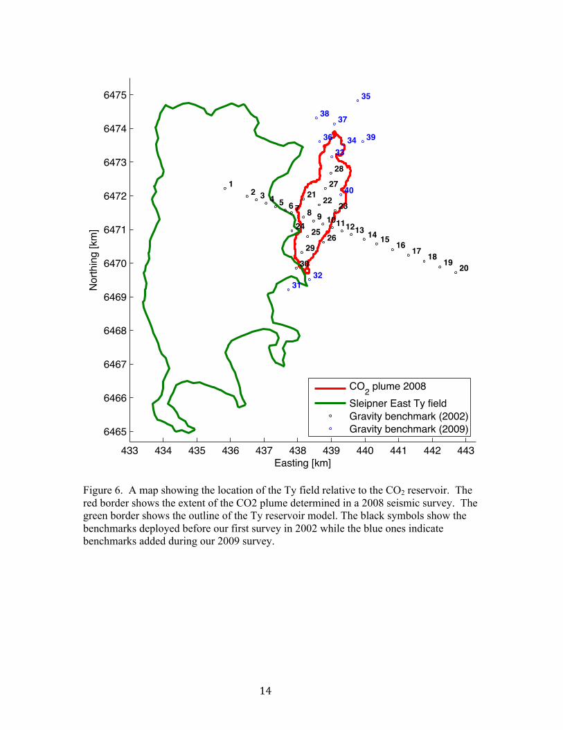
change computed using the software package SPOTL (Agnew, 1996 and 1997). This computes the effects on gravity from tidal Earth deformation and the associated crustal loading from ocean tides. We take the additional step of using the fixed-station pressure records to compute the direct attraction of a varying water level above the observation points. This methodology has been tested previously with a year long deployment of a fixed-station seafloor gravity meter (Sasagawa et al., 2008). Drift. After tidal corrections are made we compute a drift correction for each sensor (both the gravity meters and the pressure gauges drift slightly with time). This correction is based on the assumption that the tidal-corrected values of gravity and pressure do not change during the week-long period of the survey. All non-tidal changes are attributed to sensor drift (although in a few cases we find and adjust for instrument “tares” or step-changes in the instrument outputs). A variable drift rate is allowed because it is well known that the drift in quartz sensors is not linear and depends partly on ambient temperature. Drift rates and a few tares are adjusted to minimize the residuals in repeated measurements (these are shown in Figures 4 and 5). The scatter in these plots reveals the quality of the measurements within a particular survey. Benchmark shifts. Using the pressure measurements we can determine benchmark height changes that accumulate from one survey to the next. We have observed such changes at the 10 cm level among many of the Sleipner benchmarks. We have not seen similar benchmark height changes in any of our other surveys – we postulate that the vertical motions at Sleipner are from scouring of the sediment beneath the benchmarks. The survey points are relatively shallow (around 100 m) so that currents associated with storms at the surface can be significant. (All of the other survey fields are much deeper). We are confident that the benchmark height changes are real because they produce a slight gravity change as well, and correcting the gravity values for these height changes significantly reduces noise in the gravity differences between repeat surveys. Ty formation signal. As mentioned above, there is a significant gravity signal caused by the flood of water into the nearby Ty natural gas reservoir as gas is withdrawn. Figure 6 is a map view showing the location of the Ty field. Fortunately, the reservoir is quite deep (2500 m) and consequently the gravity variation observed at the seafloor due to density change in the Ty reservoir is very smooth (i.e., long wavelength) compared to the CO2 signal. Figure 7 shows the gravity signal estimated from a proprietary reservoir model of the Ty field as well as the observed gravity changes between 2009 and 2002. Figure 8 shows the gravity profile corrected for the long wavelength Ty signal. Any deviation from zero is attributed to either noise in the measurements or the addition to CO2 to the reservoir between 2009 and 2002. There is a clear signal from the decreased average density in the CO2 reservoir caused by the injected gas displacing pore water. This is the MVA signal that is the goal of the project.

8  

Results and discussions The three dimensional geometry of the CO2 bubble has been determined by repeated seismic measurements over the life of the sequestration project (Arts et al., 2008). By varying the density inside the seismically determined gas volume, we can compute the gravity effect that should be observed at the seafloor. The CO2 density that best matches the gravity observations is 720 ± 80 kg/m3. This is in reasonably good accord with the CO2 density estimated from the temperature profile within the Utsira formation (based on measurements in a well 10 km away) and laboratory characterization of CO2 gas. The density estimated in this way is 625 ± 20 kg/m3. The uncertainties in these values have been determined in several ways. The quality of the gravity values themselves are revealed by: the internal consistency of the measurements in a single survey, the repeatability of values at benchmarks away from the CO2 gas plume from survey to survey, and the results of similar surveys at other fields. We believe the uncertainties of the corrected gravity differences (survey to survey) is 2.7 microGal. The uncertainty from the Ty model can be significant, however because it is such a long wavelength signal it is actually fairly inconsequential to the final result (adjusting parameters of the Ty model essentially adds a slope to the gravity difference plotted in Figure 8 and does not have an impact on the CO2 density estimate). The sought after MVA gravity signal has an amplitude of about 12 microGal, giving a signal to noise ratio of slightly over 4. The strong spatial correlation between the observed gravity changes and the seismically determined CO2 bubble, and observations at multiple stations on the seafloor gives us confidence in the result. (Further details are in Alnes et al., 2011). Conclusion Several key conclusions can be drawn from this study: 1) Time lapse gravity measurements are an effective means for detecting and tracking

sequestered CO2. 2) The spatial distribution of observed gravity change is in good agreement with the

seismically determined shape of the CO2 bubble in the Utsira formation. 3) The good agreement between the density determined by the gravity measurements

and that determined from knowledge of reservoir temperature and pressure and known CO2 behavior indicates that the CO2 remains stable in the reservoir.

With time it is expected that the CO2 gas will interact with the formation and form carbonate material. The rate at which this occurs is not known. As it proceeds we will begin to see a discrepancy between the gravity determined density and the density expected from the reservoir conditions. The current level of agreement indicates that if such interaction has occurred at all it has proceeded slowly. As more gas is sequestered, the size of the signal will increase. We have also been

9  

learning how to improve the precision of seafloor gravity measurements (the last decade has seen nearly an order of magnitude improvement). Consequently the signal to noise ratio in future surveys will improve allowing even better quantification of the fate of sequestered CO2. Acknowledgements Our colleagues from Statoil, Håvard Alnes, Ola Eiken, and Torkjell Stenvold, led the data analysis. We are grateful to the crew of the M/V Seabed Worker for their skill in deploying the gravity sensors on the seafloor.

10  

Graphical Materials

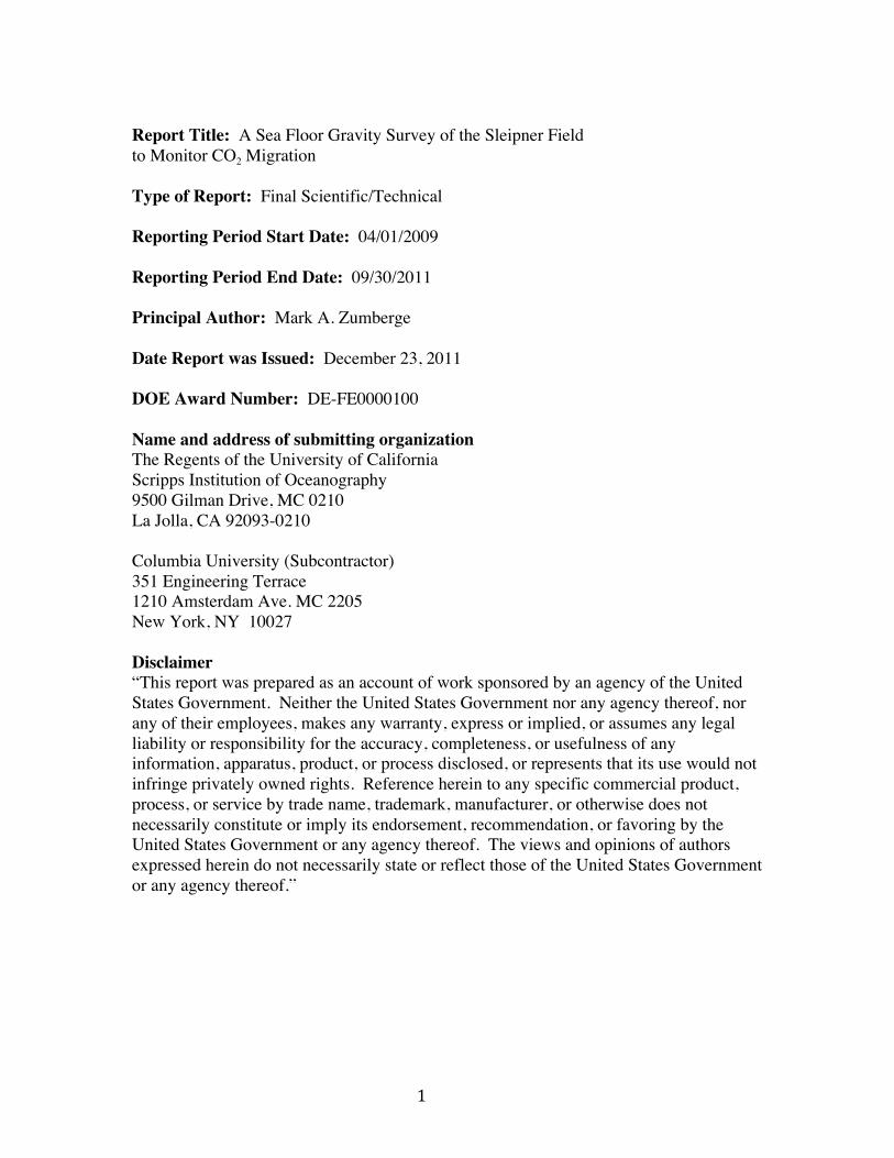
Figure 1. Map showing survey location.

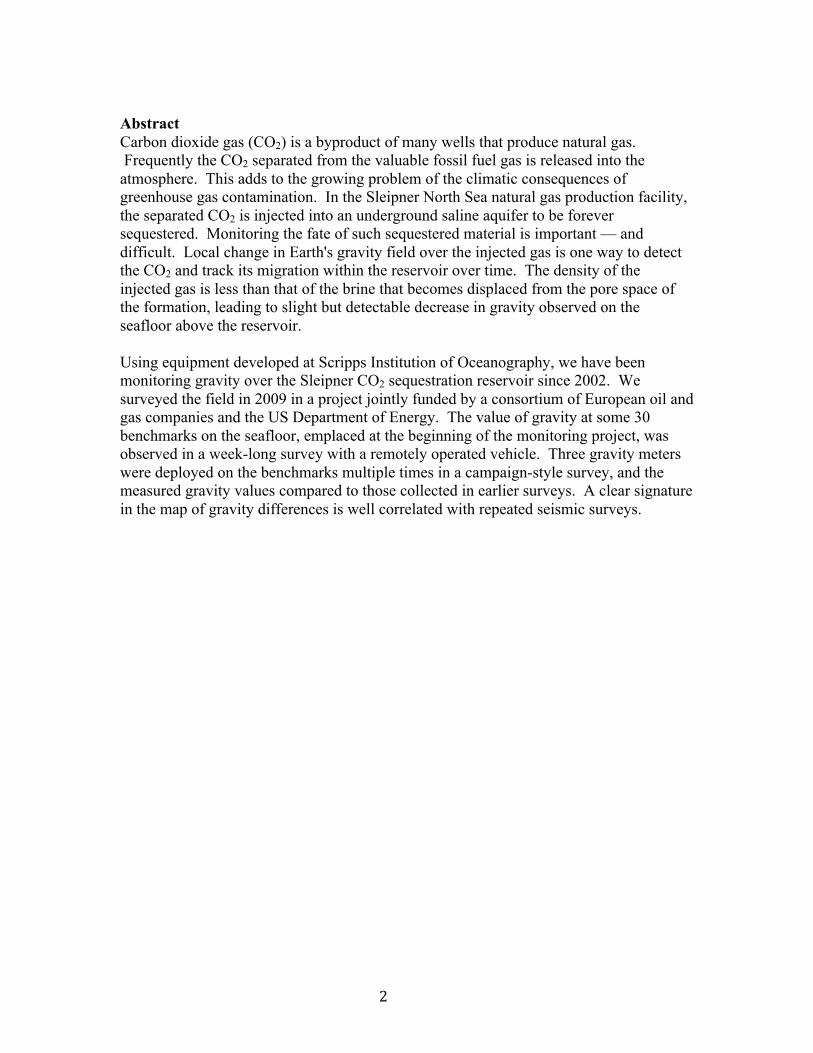
Figure 2. Map showing the layout of benchmarks on the seafloor. The blue region is the seismically determined extent of the sequestered CO2.

11  

Figure 3. The ship and ROV as it is being launched with the gravity sensing package held in a hydraulic launch arm. (The photograph was taken from a small boat near the ship).

12  

Figure 4. Repeatability of gravity measurements during the 2009 Sleipner gravity survey. Each color represents measurements taken on one of 40 benchmarks (an additional 10 benchmarks were added in the 2009 survey). The gap in the center is the result of bad weather that prohibited launch of the ROV. Each point is plotted with mean of all measurements taken at that benchmark (at least three measurements at each benchmark) removed.

187 188 189 190 191 192 193 194 1956

4

2

0

2

4

6Gravity repeatability 2.19 µGal

µG

al

Decimal day 2009

11011121314151617181922021222324252627B282933031323334353637383944056789

13  

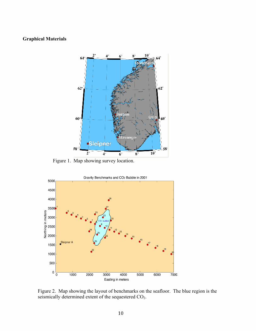
Figure 5. Repeatability of pressure (height) measurements during the 2009 Sleipner gravity survey. 0.01 kPa corresponds to a height change of 1 mm.

187 188 189 190 191 192 193 194 1950.08

0.06

0.04

0.02

0

0.02

0.04

0.06

0.08Pressure repeatability 0.028 kPa

kPa

Decimal day 2009

11011121314151617181922021222324252627B282933031323334353637383944056789

14  

Figure 6. A map showing the location of the Ty field relative to the CO2 reservoir. The red border shows the extent of the CO2 plume determined in a 2008 seismic survey. The green border shows the outline of the Ty reservoir model. The black symbols show the benchmarks deployed before our first survey in 2002 while the blue ones indicate benchmarks added during our 2009 survey.

433 434 435 436 437 438 439 440 441 442 4436465

6466

6467

6468

6469

6470

6471

6472

6473

6474

6475

12 3 4 5 6 7 8 9 10111213 14 15

1617

1819 20

2122 23

2425

26

27

28

29

30

3132

3334

35

36

3738

39

40

Easting [km]

North

ing

[km

]

CO2 plume 2008Sleipner East Ty fieldGravity benchmark (2002)Gravity benchmark (2009)

15  

Figure 7. The gravity profile corrected for everything except for the signal from the Ty field. The data are plotted with respect to benchmark number, but spaced such that they also represent position along the main survey array profile (benchmarks 1 through 20 span a distance of 7.5 km). Benchmarks 21 through 30 are off the main axis so are, in essence, separate profiles. The red points show the observed gravity changes between 2009 and 2002, the blue symbols show the expected signals from the ongoing Ty reservoir gas production, and the black symbols indicate the best fitting model that includes the gravity signals from both the CO2 and the Ty reservoir.

1 3 5 7 9 11 13 15 17 19 20 21 22 23 24 25 26 28 29 300

10

20

30

40

50

60

Benchmark no.

Gra

vity

signa

l [µ

Gal

]

ObservedWater influx + CO2 plumeWater influx

16  

Figure 8. The gravity profile after removal of the Ty field modeled signal (the difference between the black and blue traces in Figure 7.) The red symbols are the observations and the black line shows the best fitting model of CO2 density.

1 3 5 7 9 11 13 15 17 19 20 21 22 23 24 25 26 28 29 30-15

-10

-5

0

5

10

Benchmark no.

Gra

vity

signa

l [µ

Gal

]

ObservedCO2

17  

References Agnew, D. C., 1996, SPOTL: Some programs for ocean-tide loading, SIO Reference Series 96-8, Scripps Institution of Oceanography. Agnew, D. C., 1997, NLOADF: a program for computing ocean-tide loading, Journal of Geophysical Research, 102, 5109-5110. Arts, R., Chadwick, A., Eiken, O., Thieau, S., Nooner, S., “Ten years’ experience of monitoring CO2 injection in the Utsira Sand at Sleipner, offshore Norway.” First Break 26, 65-72, 2008 Alnes, H., Eiken, O., Nooner, S., Sasagawa, G., Stenvold, T., and Zumberge, M., “Results from Sleipner gravity monitoring: updated density and temperature distribution of the CO2 plume.” Energy Procedia 4, 5504-5511 (2011) doi 10.1016/j.egypro.2011.02.536, GHGT-10 Conference, 19-23 Sept 2010, RAI, Amsterdam, The Netherlands. Carbon Sequestration Atlas of the United States and Canada, 2010, third edition, US Department of Energy, National Energy Technology Laboratory. Sasagawa, G., Zumberge, M., Eiken, O., “Long term seafloor tidal gravity and pressure observations in the North Sea: Testing and validation of a theoretical tidal model.” Geophysics 73 No. 6 (2008): WA143-WA148. Zumberge, M., Alnes, H., Eiken, O., Sasagawa, G., Stenvold, T., “Precision of seafloor gravity and pressure measurements for reservoir monitoring.” Geophysics 73 No. 6 (2008): WA133-WA141. List of Acronyms and Abbreviations CCS   Carbon  capture  and  storage  CO2   Carbon  dioxide  microGal   microGal  is  the  unit  of  gravity  and  equals  10−6  Gal;  1  Gal  =  1  cm/s2  acceleration       (the  nominal  value  of  gravity  at  the  Earth’s  surface  is  about  980  Gal)  MVA   Monitoring,  verification,  and  assessment  ROV   Remotely  operated  vehicle  SPOTL   Some  programs  for  ocean  tide  loading