renovation explicit dynamic procedures by application of

International Journal of the Physical Sciences Vol. 6(2), pp. 255-266, 18 January, 2011 Available online at http://www.academicjournals.org/IJPS DOI: 10.5897/IJPS10.660 ISSN 1992 - 1950 ©2011 Academic Journals

Full Length Research Paper

Renovation explicit dynamic procedures by application of Trujillo algorithm

H. Hashamdar*, Z. Ibrahim, M. Jameel and H. B. Mahmud

Department of Civil Engineering, University of Malaya, Kuala Lumpur, Malaysia.

Accepted 31 December, 2010

In this paper, a Trujillo algorithm method for the exact solution of nonlinear explicit dynamic problems is developed. This method associates numerical techniques and it is applied to determine the natural frequencies of structures. The numerical predictions of the natural frequency are compared to analytical and experimental results. There was no direct method available for solving such a problem efficiently in the case of explicit dynamic analysis. The Trujillo algorithm is an indirect method and the approach is based upon the principle of conservation of energy. It is believed that the proposed method provides a powerful engineering tool in the analyzing of structures. Key words: Nonlinear dynamic response, optimization of energy, explicit dynamic analysis, finite element method, vibration, perturbation technique, analyzing modal, Trujillo algorithm method.

INTRODUCTION The modal dynamics procedure is suitable only for linear problems. When nonlinear dynamic response is of interest, the equation of motion must be integrated directly (Belytschko, 2008; Uksun, 2009). The direct- integrations of equation of motion is performed by using an explicit dynamic procedure. And this procedure can be an effective tool for solving a wide variety of nonlinear solid and structural mechanism problems, however, the method require a small time increment size that depends solely on the highest natural frequencies of the model and is independent of the type and duration of loading. So that the method analyze is not well suited to low-speed dynamic event and explicit method is computationally intensive and are more expensive than the modal methods (Da Silva, 2008). In this paper, nonlinear dynamic response can be found by combining a Trujillo algorithm method into explicit dynamic analyzes. When this procedure is used, the mass, the damping, and stiffness matrix matrices are assembled and the equation of dynamic equilibrium is solved at each point in time. The cable structure is considered for experimental and analytical tests. *Corresponding author. E-mail: [email protected].

There are three source of nonlinearity in structural mechanics simulation:

(i) Material nonlinearity (ii) Boundary nonlinearity (iii) Geometric nonlinearity

Geometric nonlinearity is related to changes in the geometry of the model during the analysis (Stefanou, 2009).

Cable structures are very light and flexible and they undergo appreciable deflections when subjected to external loading. Since all the main load-carrying members in cable structures are usually in tension, if the tip deflection is small, the analysis can be considered as being approximately linear. However, if the tip deflection is large, the shape of structure and, hence, its stiffness changes, then, structural mechanism will belong to nonlinearity behavior. Thus, cable structure belongs to geometrically nonlinearity groups (Huu-Tai, 2010).

Although a number of method have been developed for dynamic response analysis of structural system, but there are only a few methods which can be used for nonlinear dynamic response analysis.

Tension roof structures are analyzed for static loads and their dynamic response is checked to ensure that the design provides sufficient safety and structural

256 Int. J. Phys. Sci.

q-1

q

j

1

2

Figure 1. General view number of members to cable joints.

Figure 2. Geometric representation for a function of two variables in kinematic condition.

serviceability. Although cable structures, under service loads, exhibit nonlinear behavior, recent developments on computing methods have made it possible to carry out the analysis with great accuracy (Jian, 2007; Laie, 2010). EQUATION OF MOTION FOR A SYSTEM The cable structure is a multi degree system and the equation of motion for a multi degree of freedom (MDOF) system can be written as:

M + C (t) + K (t) x = P (t) (1)

where M= Mass matrix C (t) = Damping matrix K (t) = Stiffness matrix

x = Displacement vector x’ = Velocity vector x’’ = Acceleration vector P (t) = Load vector The assumption of a constant mass in the case of both MDOF systems is arbitrary as it could be represented as a time varying quantity.

Since m is a non-zero constant value, both sides of Equation (1) can be divided by m, and for

P=

Q=

F=

Equation (1) can be written as:

Hashamdar et al. 257

Figure 3. The direction of descent vector.

+ P +QX=F (2)

The mathematical solution of Equation (2) depends on the values of P, Q and F. Equation (2) is a linear differential equation if P and Q are independent of x and remains so even if P and Q are functions of t.

The solution is normally given in the form x = f (t) and gives exact values of x for any t. once f (t) is defined x can be derived by differentiation. When P and Q are functions of x, Equation (2) becomes non-linear (Liqus, 2003).

For such equation the solution cannot be expressed in functional form and it is necessary to plot or tabulate to solution curve point by point, beginning at (t0 , x0) and then at selected intervals of t, usually equally spaced, until the solution has been extended to cover the required range. Thus the solutions of non-linear equations require a step-by-step approach and are normally based on the use of interpolation or finite difference equations. The independent variable t is divided into equal intervals , over the range of the

desired solution. Thus the variables after n and (n+1) intervals are given by tn = n * and tn+1= (n+1)

respectively. At time tn it is assumed that the values of all the parameters are known as well as the values for same parameters at all previous intervals (n-1),(n-2),…..,2,1. At time tn+1 it is assumed that the values of the variable parameters are not known and that the purpose of the analysis is to find the value of xn+1 (in the case of MDOF system, Xn+1) and its derivatives which satisfy

M n+1+ Cn+1 n+1+kn+1xn+1= pn+1 (3)

At time tn and time tn+1 =tn+∆t the condition of dynamic equilibrium requires respectively that:

nnnnnn pxkxcxm =++••

' (4)

and

111111

' +++++

••

+ =++nnnnnn

pxkxcxm (5)

XXXnn

∆+=+1 (6)

•••

+ ∆+= XXXnn 1

••••••

+ ∆+= XXX nn 1

CCC nn ∆+=+1

KKKnn

∆+=+1 Equation (5) may be written as

M∆x n + Cn∆x n + Kn∆xn +R2 = R1 (7)

Evaluation of these expressions at the end of the time interval when t=∆t leads to the following expressions for the incremental velocity and displacement (Ghafari, 2008):

nn xxt

xt

x•••••

−∆∆

−∆∆

=∆ 366

(8a)


nn xt

xxt

x•••• ∆

−−∆∆

=∆2

33 (8b)

In general it has been found to be convenient to use the incremental displacement as the basic variable and

hence the ∆x and ∆x in terms in terms of ∆x. Rearranging Equations (8a) and (8b) yields.

txtxx n ∆∆+∆=∆•••••

2

1 (9a)

22

6

1

2

1txtxtxx nn ∆∆+∆∆+∆=∆

••••• (9b)

Substitution of Equations (9a) and (9b) into Equation (7) and assuming K and C remain constant during the time interval leads to:

(10) )2

3(

)36

()36

(

1Rx

txC

xxt

mxkxt

xt

m

nn

nn

+∆

+

++∆∆

=∆+∆∆

+∆∆

•••

••

TRUJILLO'S METHOD Trujillo presented an explicit algorithm for the dynamic response analysis of structural system. For linear undamped systems the method was shown to be unconditionally stable. An algorithm based upon the Trujillo's method has been developed for non-linear systems by Thomas (Thomas, 1981) but does not take into account the effect of damping.

The Trujillo algorithm Trujillo splits the stiffness and damping matrices into upper and lower triangular forms, as indicated below, by the subscripts U and L respectively and presents, without giving the development of the equations, the following algorithm which is divided into a forward and a backward substitution. Forward substitution:

( ) [ ]

+∆

+∆

−

∆++

∆−

∆+

∆+

∆+=

+

•

−

+

nnnUL

nUL

LLn

PPt

Xt

CCt

M

XKt

Ct

M

Kt

Ct

MX

1

2

2

12

21

1624

82

.

82 (11)

•

++

•

−∆

−= nnn

n Xt

XXX4

212

1 (12)

Backward substitution:

( ) [ ]

+∆

+∆

−

∆+

+

∆−

∆+

∆+

∆+=

++

•

+

−

+

nnnLU

nLU

UUn

PPt

Xt

CCt

M

XKt

Ct

M

Kt

Ct

MX

1

2

21

21

2

12

1

1624

82

.

82 (13)

21

2111

4+

•

+++

•

−∆

−= n

nnn Xt

XXX (14)

An advantage of this algorithm is that, since it is restricted to the use of diagonal mass matrices only, the

coefficient matrices of 2

1+nX and

1+nX are obtained

respectively in upper and lower triangular forms. Thus the solution of the equations at time

21+n

t is reduced to

forward and at time 1+nt to backward substitution only.

The Trujillo suggests two ways of splitting the stiffness and damping matrices.

The first is a symmetric splitting which satisfies the conditions:

T

ULUL KKKKK ==+ ; (15)

and

T

ULul CCCCC ==+ ; (16)

The second way differs from the first only by the manner in which the diagonal elements are distributed. Trujillo (1977), who extended Trujillo's work to apply to non-linear systems, but excludes damping and thus reduces the equilibrium equations at the n

th step to,

nnn PRXM =+••

(17)

where n

R

is internal force vector, and presents the

following algorithm for the middle and the end of step:

∆+

∆−

∆

−

∆+=

•

−

+

•

nn

nL

Ln

Pt

Rt

XKt

M

Kt

MX

22

8.

8

2

.

12

21

(18)

−

∆+= +

•••

+2

12

1

4nnnn XX

tXX (19)

∆

+∆

−

∆

−

∆+=

+++

•−

+

•

21

212

1

2

.

12

21

228.

4 nnnUUn P

tR

tXK

tMK

tMX

(20)

+

∆+= +

•

+

•

++ 1

21

211

4nn

nn XX

tXX (21)

Non-linearity is taken into account by updating the stiffness matrix at the end and if necessary also at the middle of each time step (Trujillo, 1977). Expression total potential energy

The total potential energy is written as:

W=U+V (22)

where W= the total potential energy U= the strain energy of the system, and V= the potential energy of the loading. Taking the unloaded position of the assembly as datum,

jiji

i

j

j

n

m

n

XFUW ∑∑∑===

+=3

111

(23)

where m= Total number of members, J= Total number of cable joints, Fji= External applied load on joint j in direction i, and Xji= Displacement of joint j in direction i.

The condition for structural equilibrium is that the total potential energy of the system is a minimum, that is, (kirsch, 2006).

)3,2,1(&),...2,1(0 ===∂∂ ijjXW ji (24)

The correct value of X for which W is a minimum, that is, g=0 can now be found by the iterative process

)()()()1( kjikkjikji VSXX +=+ (25)

where the suffices (k) and (k+1) denote the (k)th and (k+1)th iterate, respectively and;


where jiV = the element of the direction vector, and S

)(k=

the steplength which defines the position along

)(kjiV where the total potential energy is a minimum.

The expression for

jiV given by:

)1(

)1()1(

3

11

)()(

3

11

)()( −

−−

==

==

∑∑

∑∑+−=

kji

kjikji

i

J

j

kjikji

i

J

j

kjikjiV

gg

gg

gV (26

The stationary point in the direction of descent can be found by expressing the total potential energy as a

function of the step length alongji

V . Thus the required

value of S)(k can be determined by the condition (Uksun,

2009).

0)()(

=∂∂ kk SW (27)

In the convergence energy the iteration and tolerance are not required and the kinematic condition at one increment to calculate the kinematic condition at the next increment.

Numerical and experimental testing

The development of a mathematical control to ensure stability when using larger time steps is desirable. The use of larger time steps would mean that the starting point at the beginning of each time step would be further removed from the position where the total potential dynamic work is a minimum and thus probably lead to more iteration per time step. The mathematical model chosen was a 7*5 flat net with 105 degrees of freedom. The 7*5 net was also built as an experimental model and tested in order to verify the static and dynamic nonlinear theories given in this renovation of explicit analysis. The model, of which a diagram is given in Figure 4 and a general view in Figure 5, consisted of a 7*5 cable net, with the cables at 500 mm intervals, in which the cables were 15.24 mm diameter. At the points of intersection the cables were clamped together with thin wires. The cable net was contained within a 4 m by 3 m rectangular steel frame made.

Each steel cable was initially tensioned to around 1 kN and then left for two weeks to permit the individual wires in the strands to bed in. the cables were readjusted to 11.5 KN. This tension was maintained and checked at intervals throughout the test programme. The “wedge and barrel” was used on hollow cylindrical steel to provide Endcaster degree of freedom to boundary condition of


Figure 4. Diagram of steel frame made.

Figure 5. General view of steel frame mode.

cables. The erected rectangular net had the specifications shown in Table 1. The values in Table 1 for tensile strength and Young’s modulus were obtained after testing in laboratory.

The mass density influence the stability limit, under some circumstance scaling the mass density can potentially increase the efficiency of an analysis and the explicit dynamic uses a central difference rule to integrate


Table 1. The erected rectangular net specifications.

Specification Values

Overall dimensions 3000*4000 mm

Spacing of the cables 500 mm

Number of free joints 35

Number of fixed boundary joints 24

Number of links 82

Cables: Cross-sectional area 142.9 mm2

Young’s modulus 192.60 KN/ mm2

Breaking load 272.89 KN

Y/Strength 244.40 KN

Pretension 11500 N/link

Diameter 15.24 mm

Table 2. Degree of symmetry about the major, minor axes, deflections due to concentrated load on Node 18.

Load(N) = 2400 Theoretical (T) Experimental (E) ( T – E ) / T*100

Z Axis deflections(m), Node 18 (LVDT) 178.6E-03 177.6E-03 0.56

Z Axis deflections(m), Node 11 (LVDT) 129.3E-03 127.9E-03 1.08

Strain gage(µE),Element 16 (vertical) on cable 6.416E-06 6.255E-06 2.51

Strain gage(µE),Element 44 (vertical) on cable 21.12E-06 20.65E-06 2.23

strain gage(µE),Element 15 (vertical) on cable 6.43E-06 6.12E-06 4.82

strain gage(µE), Element 45 (vertical) on cable 21.15E-06 20.44E-06 3.36

Z axis deflections(m),Node 4 (LVDT ) 50.75E-03 50.11E-03 1.26

Z Axis deflections(m),Node 25 (LVDT) 127.9E-03 127.15E-03 0.59












the equation of motion explicitly through time. The deflections due to concentrated load on Joint 18 are shown in Figure 7.

Degrees of symmetry about the major, minor axes are investigated by deflections due to concentrated load on Node 18 is shown in Table2. The investigation consisted of checking the degree of symmetric behavior about the major and minor axes. The degree of symmetric behavior about the minor axis was investigated by first placing an increasing load on Joint 11 and then comparing the resultant displacement with those obtained by placing similar loads on Joint 25. The degree of symmetric

behavior about the minor axis was similarly studied by loading first Joint 16 and then Joint 20.

The results indicate that the percentage difference between the theoretical and experimental displacements decreases with increasing loading. For the maximum loading at 18 joint the percentage differences between the theoretical and experimental displacements at the joints measured ranged between 2.1 and 5.3%. Figure 8 shows the relationship between loads and deflection about the major axis. When the concentrated load is placed on Node 20, the deflection gradually increased from 5.35 E-3 units of deflection on Node 15 until it


Figure 7. Deflections due to concentrated load on Joint 18.

15 16 17 18 19 20 21

Load on Node 16 6.07E 1.27E 1.13E 7.45E 4.11E 1.83E 5.35E

Load on Node 20 5.35E 1.83E 4.11E 7.45E 1.13E 1.27E 6.07E

0.00E+00

2.00E-02

4.00E-02

6.00E-02

8.00E-02

1.00E-01

1.20E-01

1.40E-01

De

fle

ctio

n

Figure 8. Degree of symmetric about major axis when the load is placed on Nodes 16 and 20.


4 11 18 25 32

Load on Node 17 4.30E-02 1.04E-01 1.36E-01 1.04E-01 4.30E-02



0.00E+00

2.00E-02

4.00E-02

6.00E-02

8.00E-02

1.00E-01

1.20E-01

1.40E-01

1.60E-01

1.80E-01

2.00E-01

Def

lect

ion

Figure 9. Degree of symmetric about minor axis when the load is placed on Nodes 17 and 19.

reached a peak of 1.27E-1 on Node 20. From this point onwards, it is projected to drop sharply until it reached 6.07 E-2 on Node 15. When concentrated load is placed on Node 16, the deflection from about 6.07 E-2 units on Node 15 rapidly rose to reach a peak of 1.27 E-01 on Node 16. From this point onwards, it is project to fell slightly until it reached 5.35 E-3 units on Node 21.

The damping matrix for the proposed theory is calculated separately and its calculation does not affect the formulation of the theory in present form. The energy lost in vibration is due to work done by forces resisting the motion. A general orthogonal damping matrix can be shown to be of the from

[ ] ∑∑ ≡=−

b

b

b

b

b CkMaMC1 (28)

b

n

b

b

n

n a2

2

1ω

ωε ∑=

(29)

where =nε the damping ratio for mode n, and

=nω the frequency of mode n.

Rayleigh damping which is given by

KaMaC10

+= (30)

and in which

0a and

1a are arbitrary proportionality

factors, as contained in Equation (30) and satisfies the orthogonality conditions with regard to both the mass and

stiffness. The use of value Rayleigh damping assumes that the damping ratios in all modes can be expressed by the relationship

( )nnn aa ωωε10

/2

1+= (31)

Figure 9 shows that when the concentrated load was placed on Node 18, the deflection soared between Nodes 4 and 18 from 5.08E-2 until 1.79E-1. From this point onwards, it is projected to decline slightly to reach 5.02E-2 on Node 32. Difference of deflection in minor and major axes is synchronization.

A mode shape describes the expected curvature of a surface vibrating at a particular mode. Modes shape 1 and 2 are shown in Figures10 and 11.

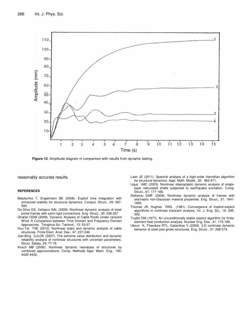
Figure 12 shows that increases in degree of freedom in Trujillo algorithm are slowly and changes in degree of freedom are reasonable.

1. Newton-Raphson method (linear) 2. Newton-Raphson method (nonlinear) 3. Trujillo algorithm method (linear) 4. Trujillo algorithm method (nonlinear)

The percentage differences between the theoretical and numerical testing results did not in any case exceed 10% and this is acceptable. The time increment used in this renovation was being smaller than the stability limit of the central-difference operator. The use a small enough time increment will result in an unstable solution. When the solution becomes unstable, the time history response of solution variable such as displacements will usually


Figure 10. 7*5 flat net, Mode 1.

oscillate with increasing amplitude and also the mass scaling was controlled by time incrimination. CONCLUSIONS The object of this work was principally to develop a explicit dynamic analysis theory and verify the theory by numerical and excremental testing.

The proposed method was found to be stable for time

steps equal to less or less than half the smallest periodic time of the system. The numerical experimentation and experimental testing c by static and dynamic testing of flat net showed a good agreement between the numerical experimentation results and the theoretically predicted values. The Turjillo method founds that method converged rapidly near the solution.

Finally the comparison of experimental and theoretically predicted values showed that the deflection calculated by the proposed nonlinear method gives


Figure 11. 7*5 flat net, Mode 2.


Time (s)

A

mp

litud

e (

mm

)

Figure 12. Amplitude diagram in comparison with results from dynamic testing.

reasonably accurate results. REFERENCES Belytschko T, Engelmann BE (2008). Explicit time integration with

enhanced stability for structural dynamics. Comput. Struct., 29: 587-590.

Da Silva GS, Vellasco SAL (2008). Nonlinear dynamic analysis of steel portal frames with semi-rigid connections. Eng. Struct., 30: 256-257.

Ghafari OGM (2008). Dynamic Analysis of Cable Roofs Under ransient Wind: A Comparison between Time Domain and Frequency Domain Approaches. Tsinghua Sci. Technol., 13: 53-57.

Huu-Tai TSE (2010). Nonlinear static and dynamic analysis of cable structures. Finite Elem. Anal. Des., 47: 237-246.

Jian-Bing CJLOK (2007). The extreme value distribution and dynamic reliability analysis of nonlinear structures with uncertain parameters. Struct. Safety, 29: 77-79.

Kirsch MB (2006). Nonlinear dynamic reanalysis of structures by combined approximations. Comp. Methods Appl. Mech. Eng., 195: 4420-4432.

Laier JE (2011). Spectral analysis of a high-order Hermitian algorithm for structural dynamics. Appl. Math. Model., 35: 965-971.

Liqus JMC (2003). Nonlinear elastoplastic dynamic analysis of single-layer reticulated shells subjected to earthquake excitation. Comp. Struct., 81: 177-188.

Stefanou GMF (2009). Nonlinear dynamic analysis of frames with stochastic non-Gaussian material properties. Eng. Struct., 31: 1841-1850.

Thomas JR, Hughes RAS (1981). Convergence of implicit-explicit algorithms in nonlinear transient analysis. Int. J. Eng. Sci., 19: 295-302.

Trujillo DM (1977). An unconditionally stable explicit algorithm for finite-element heat conduction analysis. Nuclear Eng. Des., 41: 175-180.

Uksun K, Theodore RTL, Galambos V (2009). 3-D nonlinear dynamic behavior of steel joist girder structures. Eng. Struct., 31: 268-274.

renovation explicit dynamic procedures by application of

Documents