Remote Sensing of Environment 160 (2015) 180–192

Contents lists available at ScienceDirect

Remote Sensing of Environment

j ourna l homepage: www.e lsev ie r .com/ locate / rse

Tide-corrected flow velocity and mass balance of Campbell GlacierTongue, East Antarctica, derived from interferometric SAR

Hyangsun Han a,b, Hoonyol Lee a,⁎a Department of Geophysics, Kangwon National University, Chuncheon, Kangwon-do 200-701, Republic of Koreab School of Urban and Environmental Engineering, Ulsan National Institute of Science and Technology (UNIST), Ulsan, Republic of Korea

⁎ Corresponding author. Tel.: +82 33 250 8587.E-mail address: hoonyol@kangwon.ac.kr (H. Lee).

http://dx.doi.org/10.1016/j.rse.2015.01.0140034-4257/© 2015 Elsevier Inc. All rights reserved.

a b s t r a c t

a r t i c l e i n f o

Article history:Received 1 July 2014Received in revised form 4 January 2015Accepted 6 January 2015Available online 10 February 2015

Keywords:Campbell Glacier TongueIce-flow velocityMass budgetFlux mass balanceBasal mass balanceTide deflection ratioCOSMO-SkyMedDInSAR

Accurate measurement of ice-flow velocity of floating glaciers is required to estimate ice mass balance fromvolume flux thinning/thickening, basal melting/freezing, and surface accumulation/ablation. We derived atide-corrected ice velocity map and mass budget of Campbell Glacier Tongue (CGT) in East Antarctica by using14 COSMO-SkyMed one-day tandem differential interferometric SAR (DInSAR) pairs obtained from January toNovember 2011. The vertical tidal deflection of CGT was estimated and removed from the DInSAR images byusing a tide deflection ratiomap generated by double-differential InSAR (DDInSAR) method. We then generatedaveraged ice-flow velocity (v map) and its standard deviation (σv map). Ice-flow velocity increased from theupper part of the grounding line (~0.20 m d−1) to the seaward edge of CGT (~0.67 m d−1) with σv less than~0.04 m d−1 in the main stream of CGT. The eastern part of CGT flows slower than the western part because itis grounded along the flow line and thus experiences severe basal drag. Flux mass balance (FMB), i.e., icethickness change by volume flux divergence, of CGT was obtained by combining the vmap and an ice thicknessvalue of 340 ± 18 m estimated by the ICESat GLAS data. We used mass conservation assumption in which totalmass balance (TMB,−6.29± 1.37 m a−1 observed by ICESat GLAS data) is attributed to FMB, basal mass balance(BMB) and surface mass balance (SMB, 0.24± 0.02m a−1). Mass loss in the freely floating zone of CGT is mainlycaused by basal melting (BMB = −144.5 ± 39.9 Mt a−1) while thinning by volume flux (FMB = −67.2 ±8.9 Mt a−1) is relatively small. In the hinge zone of CGT, mass change is contributed to FMB of −147.3 ±25.2 Mt a−1 and BMB of 15.3 ± 39.8 Mt a−1. However, basal freezing derived for the hinge zone may beerroneous as a result of the constant ice thickness assumption extrapolated from the freely floating zone.

© 2015 Elsevier Inc. All rights reserved.

1. Introduction

Outlet glaciers originate from an ice sheet and flow into the ocean toformfloating glaciers such as ice shelves and ice tongues at the terminus(Pattyn & Derauw, 2002; Rignot, 2002; Thomas, Frederick, Krabill,Manizade, & Martin, 2009). Temporal change in the thickness of thefloating glaciers influences the mass balance of the ice sheet consider-ably (Pritchard et al., 2012a; Rignot & Thomas, 2002). Total mass bal-ance (TMB) of a floating glacier is controlled by flux mass balance(FMB) defined as the ice thickness change by the lateral divergence ofice volume flux, basal mass balance (BMB) by basal melting or freezing,and surface mass balance (SMB) by surface accumulation and ablation(Pritchard et al., 2012a; Rignot & Jacobs, 2002; Rignot, Jacobs,Mouginot, & Scheuchl, 2013; Seroussi et al., 2011).

FMB is derived by flux divergence of ice-flow velocity which can beobtained by using differential interferometric synthetic aperture radar(DInSAR) with centimeter accuracy. Many studies have used DInSARanalysis to measure ice-flow velocity and mass balance of the Antarcticice shelves (Neckel, Drews, Rack, & Steinhage, 2012; Rignot, 2002;Rignot, Vaughan, Schmeltz, Dupont, & MacAyeal, 2002; Scheuchl,Mouginot, & Rignot, 2012; Wen et al., 2010; Young & Hyland, 2002).

Floating glaciers experience tidal deflection in the vertical directionas well as gravitational ice flow in the horizontal direction. As bothsignals appear simultaneously in DInSAR images (Rignot et al., 2011),the tidal deflection signal should be removed to measure accurate ice-flow velocity. As most Antarctic ice shelves and ice tongues flow veryquickly out into the ocean, DInSAR pairs with short temporal baseline,such as one-day tandem and a few days of repeat-pass, are required toavoid temporal decorrelation (Han & Lee, 2014). In such cases, theDInSAR signal from the vertical tidal deflection can be similar in magni-tude to that of ice-flow displacement, which causes significant error inthe measurement of ice-flow velocity (Legrésy, Wendt, Tabacco,Rémy, & Dietrich, 2004; Rignot, 1998).

Fig. 1. (a) COSMO-SkyMed SAR image over Campbell Glacier obtained on 27November 2011, ofwhich location is in the small red box in the upper left image. Thewhite lines represent thelocation of the grounding line (Han & Lee, 2014). The blue- and red-dotted lines represent the edge of Campbell Glacier Tongue in 1997 and 2006, respectively. A white dotted line acrossCampbell Glacier Tongue represents the orbit of the ICESat GLAS. (b) Tide deflection ratio map (α map) of Campbell Glacier Tongue generated by DDInSAR technique.

Table 1COSMO-SkyMed one-day tandem interferometric SAR pairs used in this study. B⊥ and Ṫare the perpendicular baseline of the interferometric SAR pairs and the one-day differenceof tide height predicted by the IBE-corrected Ross_Inv tide model, respectively.

ID Dates (yyyy/mm/dd) B⊥ (m) Ṫ (cm)

1 2011/01/26, 2011/01/27 18.9 −11.62 2011/02/27, 2011/02/28 5.7 −4.53 2011/03/15, 2011/03/16 −44.4 −17.54 2011/03/31, 2011/04/01 −39.2 8.35 2011/05/02, 2011/05/03 −89.6 8.36 2011/05/18, 2011/05/19 75.9 27.87 2011/06/03, 2011/06/04 −36.5 −3.38 2011/06/19, 2011/06/20 −47.5 −14.79 2011/08/22, 2011/08/23 181.7 27.610 2011/09/07, 2011/09/08 37.3 1.011 2011/10/09, 2011/10/10 −44.4 5.812 2011/10/25, 2011/10/26 −110.9 −14.013 2011/11/10, 2011/11/11 −91.7 2.014 2011/11/26, 2011/11/27 −23.4 7.5

181H. Han, H. Lee / Remote Sensing of Environment 160 (2015) 180–192

Several studies have attempted to correct the tidal effect on a fewfloating glaciers such as Ross Ice Shelf, Ronne Ice Shelf, and Amery IceShelf by using tide models (Scheuchl et al., 2012; Wen et al., 2010).However, they could not correct the detailed tidal effect, especiallywithin the hinge zone, due to the lack of information on the spatial var-iation of tidal response of the floating glaciers.

Tide deflection ratio, defined as the ratio of the vertical tidal de-flection over tide height, can be determined by double-differentialinterferometric SAR (DDInSAR) technique that differentiates twoDInSAR signals by assuming that the gravitational ice flow is con-stant during the observations (Han & Lee, 2014; Rignot, 1996;Rignot et al., 2011). It enables the estimation of the spatial variationof the vertical tidal deflection of a floating glacier as a function of tideheight, and thus the extraction of accurate ice-flow velocity fromDInSAR signals.

In this paper, we measure accurate ice-flow velocity of CampbellGlacier Tongue (CGT) in East Antarctica by removing the vertical tidaldeflection from one-day DInSAR signals, to calculate mass balance ofthe glacier tongue. Section 2 presents the study area and the datasetused in this study. Section 3 describes the methodology of the accuratemeasurement of ice-flow velocity from the DInSAR dataset and the

calculation of mass balance terms such as TMB, SMB, FMB and BMB.Section 4 presents results and discussion while Section 5 concludesthis paper.

Fig. 2. Flowchart of data processing.

182 H. Han, H. Lee / Remote Sensing of Environment 160 (2015) 180–192

2. Study area and data

2.1. Study area

Campbell Glacier (74° 25′ S, 164° 22′ E) is a fast-flowing outlet gla-cier with a length of about 110 km originating from the end of MesaRange in Victoria Land, East Antarctica (Frezzotti, 1993). It flows intothe northern Terra Nova Bay in the Ross Sea and forms an ice tongue(CGT) (Fig. 1a). CGT is composed of two ice streams: one is the mainstream in the east, 13.5 km long and 4.5 km wide, and the other is thebranch stream in the west, 8.0 km long and 2.5 km wide (Han & Lee,2014). The blue and red-dotted lines in Fig. 1a represent the edge ofCGT in 1997 observed by a Radarsat-1 SAR image (Jezek, 1999) andthat in 2006 by an ALOS PALSAR image, respectively. The ice front ofthe main stream of CGT has retreated and been chunked out 5 km byice calving between 1997 and 2011.

The gravitational ice-flow velocity of CGT has increased graduallyfrom 140 to 240 m a−1 in 1989, observed by feature tracking of theSPOT images (Frezzotti, 1993), to 181–268 m a−1 between 2010 and2011 by the offset tracking of the COSMO-SkyMed SAR images (Han,Ji, & Lee, 2013). The location of the grounding line of CGT, representedas the white lines in Fig. 1a, has retreated 0.3–1.5 km between 1996and 2011 (Han & Lee, 2014). Han and Lee (2014) also reported thatthe vertical tidal deflection of CGT amounts to 60 cm which is similarin magnitude with daily ice flow.

2.2. Data

We used 14 one-day tandem interferometric SAR image pairs overCGT obtained from January to November 2011 (Table 1) by COSMO-SkyMed satellites. The COSMO-SkyMed constellation is composed offour satellites equipped with X-band SAR (center frequency 9.6 GHz)with 16 days of repeat pass (Bianchessi & Righini, 2008; Covello et al.,2010). The COSMO-SkyMed-2 satellite revisits a ground track with thesame geometric conditions as the COSMO-SkyMed-3 satellite after one

Fig. 3. Examples of the COSMO-SkyMed one-day tandemDInSAR images rewrapped by 4π. Eachis the one-day tidal variation predicted by the IBE-corrected Ross_Inv tide model correspondin

day to obtain interferometric data (Covello et al., 2010). All SAR imageswere acquired with 3 m resolution in strip-mapmode, VV-polarization,and an incidence angle of 40° in descending orbit at around 3:45 UTC.The Global Digital Elevation Model (GDEM) with a grid spacing of30 m and the vertical accuracy of 20 m (Fujisada, Bailey, Kelly, Hara, &Abrams, 2005) from the Advanced Spaceborne Thermal Emission andReflection Radiometer (ASTER)was used to remove topographic phasesfrom the COSMO-SkyMed interferograms.

The Ross Sea Height-based Tidal InverseModel (Ross_Inv) (Padman,Erofeeva, & Joughin, 2003) was used to predict tide height at a centerpoint on CGT beyond the hinge zone. The effect of load tide wascorrected by using the TPXO6.2 Load Tide model (Egbert & Erofeeva,2002). The inverse barometer effect (IBE) of the predicted tide height,i.e., ~1 cm depression of tide height per 1 mbar increase in atmosphericpressure (Padman, King, Goring, Corr, & Coleman, 2003), was correctedby using the in situ atmospheric pressure datameasured by an automat-ic weather system installed near CGT. Han, Lee, and Lee (2013) showedthat the IBE-corrected Ross_Inv is the optimum tide model over TerraNova Bay when compared with other tide models such as CATS2008a,FES2004 and TPXO7.1, based on the fact that it has the smallest root-mean-square error of 4.1 cm between tide height predicted by themodel and that measured by a tide gauge.

Surface elevation of CGT measured by the Geoscience Laser Altime-try System (GLAS) onboard the Ice, Cloud, and land Elevation Satellite(ICESat) was used to estimate the ice thickness of CGT and to fill theDEMs of CGT that are missing in the GDEM (Han & Lee, 2014). Over anice shelf, ICESat GLASmeasures surface elevationwith the vertical accu-racy of ~14 cm over an approximately 60 m footprint and 172 m along-track spacing (Abshire et al., 2005; Schutz, Zwally, Shuman, Hancock, &DiMarzio, 2005; Shuman et al., 2006).We used 7 ICESat GLASmeasure-ments (GLA12, Release-633) of the same ground track across CGT(a white dotted line in Fig. 1a) from March 2005 to November 2008.All the ICESat GLAS datawere corrected for an error in range determina-tion from transmit-pulse reference selection. ICESat GLAS data over iceshelves are conventionally corrected for the ocean tide (Zwally et al.,

color cycle represents surface displacement of 3.1 cm in the line of sight (LOS) direction. Ṫg to each DInSAR image. The white lines represent the location of the grounding line.

183H. Han, H. Lee / Remote Sensing of Environment 160 (2015) 180–192

184 H. Han, H. Lee / Remote Sensing of Environment 160 (2015) 180–192

185H. Han, H. Lee / Remote Sensing of Environment 160 (2015) 180–192

2002), but not in CGT as the product regard it as inland. Therefore, wecorrected the tidal effect by the IBE-corrected Ross_Inv data with atmo-spheric pressure data from the ERA-Interim reanalysis by the EuropeanCentre for Medium-Range Weather Forecasts (Dee et al., 2011).

We used SMB, defined as balance between the processes of accumu-lation and ablation on ice surface, over CGT simulated by the RegionalAtmospheric Climate Model (RACMO) (Lenaerts, van den Broeke,van de Berg, van Meijgaard, & Kuipers Munneke, 2012) to calculatemass budget of CGT. RACMO provides simulation of Antarctic surfacemass balance with the horizontal resolution of ~27 km with a correla-tion coefficient of 0.88 by comparingwith the in situ SMB in the Antarc-tic Ice Sheet (Lenaerts et al., 2012). We used the averaged value of SMBfor CGT from January 1979 to July 2012.

3. Method

In this section, we describe the method used to derive a tide-corrected ice-flow velocity map, FMB map and BMB map of CGT byapplying mass conservation equations. An overview of data processingis shown in Fig. 2.

3.1. Generation of a tide-corrected ice-flow velocity map (v map)

First, we generated 14 one-day tandem differential interferogramsby removing the topographic phase using the ASTER GDEM. The verticalaccuracy of the ASTER GDEM is good enough to remove topographicphases from the interferograms with short perpendicular baselinesranging from23.4 to 181.7m (Table 1). The phase unwrappingof the in-terferograms is performed by the branch-cut algorithm (Goldstein,Zebker, & Werner, 1988).

DInSAR signals of floating glaciers (ϕLOS) represent surface displace-ment as the summation of the horizontal ice flow (ϕLOS

flow) and thevertical tidal deflection (ϕLOS

tide) in the line of sight (LOS) direction:

ϕLOS ¼ ϕflowLOS þ ϕtide

LOS: ð1Þ

A positive displacement in the LOS direction represents an increasein range from satellite to target. Vertical tidal deflection (Z) as a functionof x and y in the horizontal plane and time t can be represented as (Han& Lee, 2014)

Z x; y; tð Þ ¼ α x; yð ÞT x; y; tð Þ; ð2Þ

where α is the tide deflection ratio over tide height (T). For one-dayDInSAR signals, the one-day difference of Z is related to the one-daydifference of T, defined here as Ṫ so that

ϕtideLOS x; y; tð Þ ¼ α x; yð Þ T� x; y; tð Þ cosθ ð3Þ

where θ is the radar look angle.We used a tide deflection ratio map (α map) of CGT (Fig. 1b) to

remove the tidal signal from DInSAR images. It was generated byperforming a linear regression analysis between the DDInSAR-derivedtidal deflection and tidal variations predicted by the IBE-correctedRoss_Inv (Han & Lee, 2014). The α map clearly defines the spatialvariation of tidal response of CGT as α value increases from the ground-ing line to the seaward edge of the hinge zone. The α map has ~4% un-certainty due to Ross_Inv tide model error and the imperfect correctionof the IBE (Han & Lee, 2014).

Some examples of the COSMO-SkyMed one-day tandemDInSAR im-ages with various tidal conditions are shown in Fig. 3. The white lines in

Fig. 4. Examples of the one-day tidal deflection images of Campbell Glacier Tongue generated bydeflection ratio (Fig. 1b). Each color cycle represents tidal deflection of 3.1 cm in the LOS direc

the DInSAR images represent the location of the grounding line of CGTdefined as the zero-tide deflection ratio lines from the α map. Signalsof ϕLOS over the grounded part of Campbell Glacier represent gravita-tional ice flow only, which show very small variation in 2011. However,signals of ϕLOS over CGT, especially in the hinge zone, seem to be signif-icantly different in each of the DInSAR images due to various tidalconditions.

Fig. 4 shows some examples of the simulated ϕLOStide corresponding to

tidal conditions of the one-day tandem DInSAR images in Fig. 3. Signalsof ϕLOS

tide clearly define the grounding line, hinge zone and the spatial var-iation of tidal deflection of CGT responding to the given tidal conditions.The maximum Ṫ of 27.8 cm (Fig. 4c and ID 6 in Table 1) can bemisinterpreted as 33 cm of one-day horizontal ice flow in the DInSARimage. This error accounts for 45% of the maximum ice-flow velocityof CGT measured by the previous study (Han, Ji, et al., 2013). Therefore,signals of ϕLOS

tide should be removed from the one-day DInSAR-derivedsurface displacement over CGT to extract accurate ice-flow velocity.

We removed the signals of ϕLOStide from the DInSAR images and ex-

tractedϕLOSflow over CGT (Fig. 5). One-day ice flow over both the grounded

part of Campbell Glacier and CGT are steady with time, from which wecould confirm that the assumption of steady ice flow, used to estimate αvalues by DDInSAR, is valid.

ϕLOSflow represents an ice-flow component in the radar LOS direction.

To determine the actual ice flow in the horizontal direction, weperformed offset tracking between the two SAR images obtained on25 October and 10 November 2011. We then converted the observedice flow in the LOS direction to that in the horizontal flow direction togenerate a map of averaged ice-flow velocity (v map) and its standarddeviation (σv map).

3.2. Calculation of flux mass balance (FMB)

FMB at any point of a glacier is calculated as (Rignot et al., 2013)

FMB ¼ −∇ � Hvð Þ ¼ −H ∇ � vð Þ−∇ Hð Þ � v ð4Þ

where H is the ice thickness and v is the ice-flow velocity. FMB repre-sents ice thickness change due to horizontal compression or expansionfrom ice volume fluxmeasured inm a−1.H can be estimated by (Griggs& Bamber, 2009, 2011)

H ¼ h−δð Þρs

ρs−ρi; ð5Þ

where h is the ice surface elevation above mean sea level, δ is the firndepth correction, ρs is the sea water density (typically 1030 kg m−3),and ρi is the ice density (typically 917 kg m−3).

We used h of CGTmeasured by the ICESat GLAS from2005 to 2008.Hdeduced from the Eq. (5) is valid on ice in a hydrostatic equilibriumstate. Therefore, h values of CGT were extracted on the region where αvalue is larger than 0.96 by considering the 4% uncertainty of the αmap (Han & Lee, 2014). All h valueswere averaged to lower the randomnoises included in individual observations (Griggs & Bamber, 2011) andto find a representative H value over the whole CGT for a long-termstage. We estimated a value of 13 m for δ at CGT (Bindschadler et al.,2011; van den Broeke, van de Berg, & van Meijgaard, 2008). H value ofCGTwas found to be 340±18mbyusing h value of 50±2mmeasuredacross the freely floating zone.

The FMB calculated by Eq. (4) has errors arising fromuncertainties inice-flow velocity and ice thickness. By the assumption of constant icethickness, the second term on the right hand side in Eq. (4) is zero

using the one-day tidal variation (Ṫ) predicted by the IBE-corrected Ross_Inv and the tidetion. The white lines represent the location of the grounding line.

186 H. Han, H. Lee / Remote Sensing of Environment 160 (2015) 180–192

187H. Han, H. Lee / Remote Sensing of Environment 160 (2015) 180–192

and thus we considered the uncertainty in FMB (σFMB) for the first termonly. σFMB (in m a−1) at any point of CGT can be estimated by using theuncertainty propagation theorem by

σ FMB ¼ FMB�ffiffiffiffiffiffiffiffiffiffiffiffiffiffiffiffiffiffiffiffiffiffiffiffiffiffiffiffiffiffiffiffiffiffiffiffiffiffiffiffiffiffiffiffiffiffiffiffiffiffiffiffiffiffiffiffiffiffiffiffiffiffiffiffiffiffiσH=Hð Þ2 þ ffiffiffiffiffiffiffiffiffiffiffiffiffi

σ ∇�vð Þp

= ∇ � vð Þ� �2

rð6Þ

where σH is the uncertainty in the uniform ice thickness (±18 m) andσ(∇ ⋅ v) is the uncertainty in the divergence of ice-flow velocity derivedfrom the v map and σv map.

3.3. Estimation of basal mass balance (BMB)

We estimated the BMB of CGT by using the mass conservationequation defined as (Pritchard et al., 2012a; Rignot et al., 2013)

∂H=∂t ¼ TMB ¼ FMBþ BMBþ SMB ð7Þ

where ∂H/∂t is the total mass balance (TMB) representing the gross icethickness change rate.

A ∂H/∂t value of CGT can be estimated by using the h values mea-sured by the ICESat GLAS. We calculated an average h value for eachICESat GLAS ground-track by an assumption of constant ice thicknessover the whole CGT. We then calculated the mean ∂h/∂t from460 days to 956 days except for the reference value in 2005 and forthe final value in 2008 (Fig. 6). The horizontal bars in Fig. 6 representthe time period used to calculate the mean ∂h/∂t values. The ∂h/∂tvalues were corrected for the change in firn depth of −0.01 ±0.01 m a−1 which was interpolated from values for ice tongues nearCGT such as Drygalski Ice Tongue and Aviator Glacier Tongue(Pritchard et al., 2012b). The change in firn depthwas produced by sim-ulating firn densification rate, vertical heat transport, and meltwaterpercolation and refreezing (Pritchard et al., 2012b). We averaged themean ∂h/∂t values over the full period of the ICESat GLAS observations,which was converted to ∂H/∂t using the ρi and the ρs. ∂H/∂t of CGTwas estimated to be −6.29 ± 1.37 m a−1 (in water equivalent) fromthe ∂h/∂t value of −0.69 ± 0.15 m a−1 (Fig. 6 and Table 2). The SMBvalue of 0.24 ± 0.02 m a−1 in water equivalent (Table 2) was used forCGT.

The uncertainty in BMB (σBMB) arises from the uncertainty in TMB(σTMB), SMB (σSMB) and FMB (σFMB). At any point of CGT, σBMB

(in m a−1) is estimated as

σBMB ¼ffiffiffiffiffiffiffiffiffiffiffiffiffiffiffiffiffiffiffiffiffiffiffiffiffiffiffiffiffiffiffiffiffiffiffiffiffiffiffiffiffiffiffiffiffiffiffiffiffiffiffiffiσTMB

2 þ σ SMB2 þ σ FMB

2q

: ð8Þ

σTMB of ±1.37 m a−1 and σSMB of ±0.02 m a−1 were used to estimatethe σBMB.

The calculated BMB map inherits the advantage of the FMB mapwhichwas derived fromvery accurate ice velocitywith high-spatial res-olution by correcting tidal effect especially in the hinge zone. This is amajor improvement of this study in the estimation of the BMB overthe previous studies without adequate tidal correction (Rignot,Mouginot, & Scheuchl, 2011a; Scheuchl et al., 2012; Wen et al., 2010).However, the use of a constant ice thickness and its change, estimatedat the freely floating zone by an assumption of hydrostatic equilibrium,can induce large errors of FMB and BMB in the hinge zone. This isdiscussed in the following section.

Fig. 5. Examples of the one-day ice-flow images after removing the one-day tidal deflection (Fig3.1 cm in the LOS direction. The white lines represent the location of the grounding line.

4. Result and discussion

4.1. Ice-flow velocity of Campbell Glacier

Fig. 7a and b shows the ice velocity map (v map) and its standarddeviation map (σv map), respectively. The white solid lines representthe location of the grounding line and a white-dotted line representsthe seaward edge of the hinge zone of the main stream of CGT. Theblack arrows in Fig. 7a represent some of the ice-flow directionsestimated by the offset tracking results. Ice-flow velocity graduallyincreases from the upper grounded part of Campbell Glacier(~0.20 m d−1) to the seaward edge of CGT (~0.67 m d−1), and fromthe glacial margins to the central flow line of the glacier.

Within the hinge zone of the main stream of CGT, ice-flow velocityincreases along the flow line from grounding line (~0.52 m d−1) tothe seaward edge of the hinge zone (~0.62 m d−1). However, ice-flowvelocity of the freely floating zone of CGT is almost constant along theflow line. The eastern part of the main stream of CGT flows slowerthan the western part. This is related to the geometry of the groundingline (Han & Lee, 2014) which is parallel to the flow direction. Therefore,ice flow slows down due to basal drag (Whillans & van der Veen, 1997)in the eastern part while that of the western part increases after thegrounding line. The southwestern edge of the main stream of CGTshows the fastest ice flow although it is grounded by an underwaterridge (Han & Lee, 2014), which implies that ice flow of this area is notsignificantly resisted by basal drag and thus this ice is weakly grounded.The branch stream of CGT shows spatially irregular ice flow due to therandom motion of the broken ice chunks (Han & Lee, 2014).

Most areas of the grounded part of Campbell Glacier show small σv

less than ~0.02 m d−1, indicating that ice-flow velocity is almost steadywith time. However, some regions showσv values larger than 0.1md−1

due to the insensitivity of the DInSAR signal to the ice flow in the azi-muthal direction of the SAR coordinates. The ice-flow direction ofthose regions is almost perpendicular to the LOS direction (Fig. 7).

σv values on the main stream of CGT are ~0.04 m d−1, which aretwice the values on the grounded part of Campbell Glacier. This iscaused by either the uncertainty of the α map, especially by the errorof tide height predicted by Ross_Inv (Han & Lee, 2014), or the tide-in-duced fluctuation of the horizontal ice velocity (Marsh, Rack,Floricioiu, Golledge, & Lawson, 2013). However, the σv values of~0.04 m d−1 are equivalent to only ~6% of ice-flow velocity of CGT.Some regions of the branch stream of CGT show large σv values due torandom motion of the broken ice chunk. Therefore, we will focus onlyon the main stream of CGT for further analysis in the following section.

4.2. Flux mass balance (FMB) of Campbell Glacier Tongue

FMB (m a−1 in water equivalent) of the main stream of CGT and itsuncertainty are shown in Fig. 8a and b, respectively. The white solidlines represent the location of the grounding line and a white-dottedline represents the seaward edge of the hinge zone of the main streamof CGT. FMB varies spatially from−25 to 7 m a−1 with the uncertaintyless than 2 m a−1. Negative FMB values, representing ice thinning byvolume flux, are dominant over the glacier tongue with an averagevalue of −4.08 ± 0.51 m a−1 over the main stream of CGT (Table 2).

In the freely floating zone, FMB ranges from −7 to 7 m a−1 with anaverage of−2.08 ± 0.27 m a−1. This represents that ice thinning fromvolume flux is spatially steady due to small variation of ice flow in thefreely floating zone.

FMB in the hinge zone varies spatially, which ranges from −25 to5 m a−1 with an average value of −7.27 ± 1.24 m a−1. FMB is notice-ably high along the ice-flow lines at the central-eastern part of the

. 4) from the one-day surface displacement (Fig. 3). Each color cycle represents ice flow of

-1

-0.8

-0.6

-0.4

-0.2

0

2005/03 2006/03 2007/03 2008/03 2009/03

h/ t

(m

a−1

)

Date (yyyy/mm)

Fig. 6.Mean ∂h / ∂t of Campbell Glacier Tongue estimated from the ICESat GLAS surface el-evation data. The horizontal bars represent the time period to calculate the mean ∂h/∂tvalues. The mean ∂h/∂t values from 2005 to 2007 were averaged for the final value of∂h/∂t.

188 H. Han, H. Lee / Remote Sensing of Environment 160 (2015) 180–192

hinge zone (illustrated in purple in Fig. 8a), which results from thestrong gradient of the ice-flow velocity increasing from the easternpart to the western part of CGT. Based on the Eq. (4), FMB depends onice thickness and flow velocity, and their gradients. As we used a con-stant ice thickness, FMB of CGT is affected by the gradient of ice velocityonly. We found that the velocity gradient in thinning zones is strongerin east–west direction compared to surrounding areas causing fracturesand crevassing (Bindschadler, Vornberger, Blankenship, Scambos, &Jacobel, 1996; Harper, Humphrey, & Pfeffer, 1998; Vaughan, 1993;Vornberger & Whillans, 1986). A large number of crevasses parallel tothe flow direction by large transverse strain (Bindschadler et al., 1996;Harper et al., 1998) are observed in the area of strong ice velocity gradi-ent clearly shown in Fig. 1a.

Although the FMB map was derived from accurate ice velocity bycorrecting tidal effect onDInSAR signals, it could contain errors especial-ly in the hinge zone. This is because we used a constant ice thicknessestimated at the freely floating zone and assumed zero-gradient of icethickness. The hydrostatic equilibrium assumption may not be valid inthe hinge zone (Bindschadler et al., 2011; Griggs & Bamber, 2011;Marsh, Rack, Golledge, Lawson, & Floricioiu, 2014). Moreover, the icethickness in the hinge zone is typically thicker than that in the freelyfloating zone (Bindschadler et al., 2011; Marsh et al., 2014).

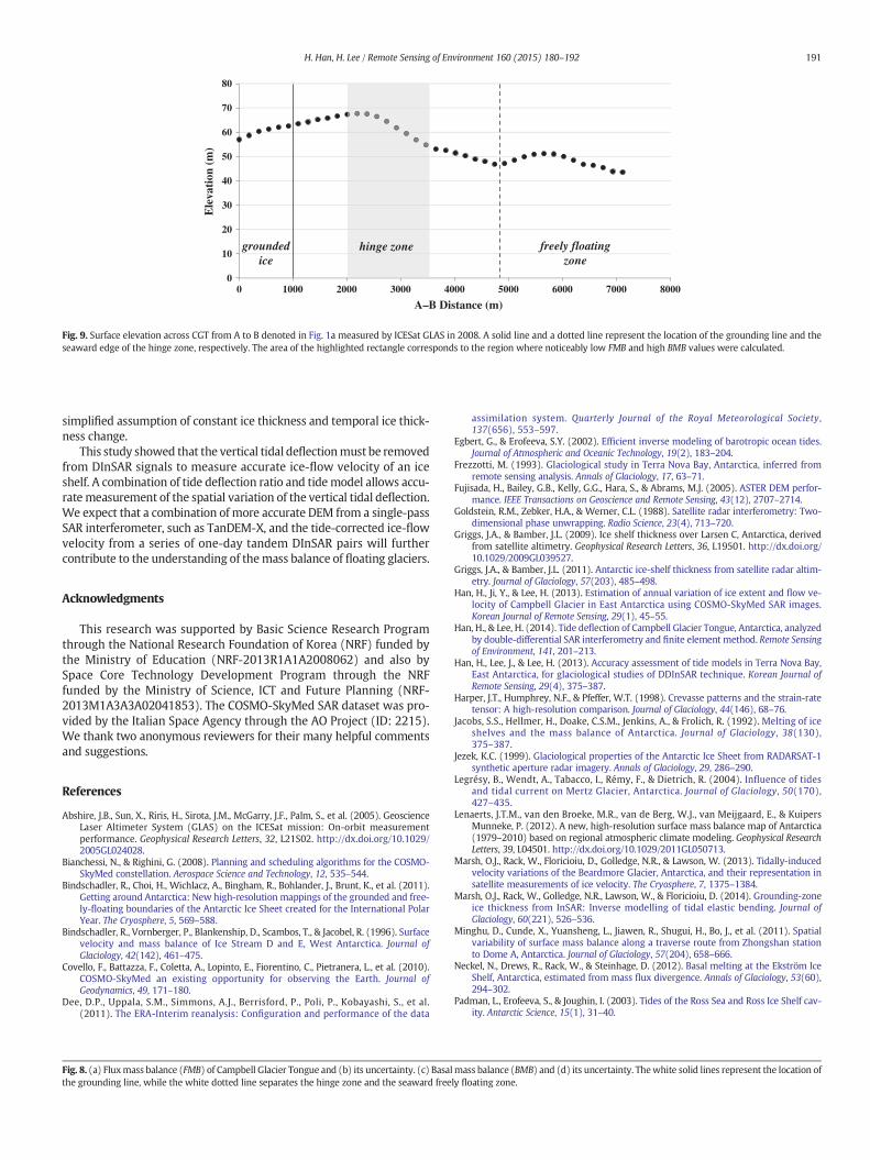
Surface elevation of CGT measured by ICESat GLAS was used toassess the effect of a likely thickness gradient on the FMB. Althoughthe assumption of hydrostatic equilibrium is invalid, we used the sur-face elevation as a proxy to qualitatively investigate a possible thicknessgradient. Fig. 9 shows surface elevation across CGT, from A to B denotedin Fig. 1a,measured from an ICESat GLAS track in 2008. A solid line and adotted line in Fig. 9 represent the location of the grounding line and theseaward margin, respectively. The surface elevation decreases down-stream, and its gradient (a negative gradient) is strong in the hingezone (~−0.01), especially in high ice thinning zone by flux diver-gence (the highlighted rectangle in Fig. 9) while that in the freelyfloating zone is relatively small. This indicates that ice thickness inthe freely floating zone is spatially homogeneous and thus the calcu-lated FMB is fairly accurate, while FMB in the hinge zone could be in-accurate due to significantly decreasing ice thickness towards theseaward edge.

Noting that ice velocity in the hinge zone is high (~230ma−1)whileits strain rate is low (less than 0.0005 a−1), the accuracy of FMB is large-ly affected by the gradient in ice thickness. A negative gradient in icethickness can augment the FMB calculated by assuming constant icethickness extrapolated from the freely floating zone. It follows that

FMB in the hinge zone of CGT calculated in this study is possiblyunderestimated.

4.3. Basal mass balance (BMB) of Campbell Glacier Tongue

BMB of the main stream of CGT estimated by the mass conservationassumption and its uncertainty (m a−1 in water equivalent) are shownin Fig. 8c and d, respectively. Most areas of CGT show negative BMBvalues, with an average of −2.46 ± 1.07 m a−1, which means that theice bottom is melting.

Bottommelting in the freely floating zone of CGT is very highwith anaverage value of−4.46± 1.24m a−1 (BMB values ranging from−10 to2 m a−1), which suggests that there was a change in warm deep-watercirculation causing the increase in basal melting of an ice shelf (Jacobs,Hellmer, Doake, Jenkins, & Frolich, 1992). It is the largest value in TerraNova Bay when compared with those estimated in the freely floatingzone of other glacier tongues such as Drygalski Ice Tongue (−3.3 ±0.5 m a−1), Aviator Glacier Tongue (−1.7 ± 0.3 m a−1), and NansenIce Sheet (−0.6 ± 0.3 m a−1) (Rignot et al., 2013). The ice thickness ofthe freely floating zone of CGT (340 ± 18 m) would be halved in fortyyears, if the high bottom melting rate (−4.46 ± 1.24 m a−1) sustains.In the freely floating zone, BMB estimated by using constant ice thicknesschange ismeant to be fairly accurate because FMB iswell determined andthe spatial variation of ice thickness change in the freely floating zone ispresumed to be insignificant from the gradient of surface elevation.

BMB valueswithin the hinge zone range from−10 to 20m a−1 withaverage value of 0.75 ± 1.96 m a−1 which represents bottom freezing(Fig. 8a). The remarkably high bottom freezing derived for the central-eastern part of the hinge zone (illustrated in red in Fig. 8c) where FMBvalues may be considerably underestimated (Fig. 8a). As theunderestimated FMB yields the exaggerated BMB by themass conserva-tion assumption, BMB values in the hinge zone of CGT could be incorrectby the overestimation. Moreover, a constant value of ∂H/∂t used in themass conservation assumption contributes the additional errors toBMB in the hinge zone because ice thickness can change spatially overthe hinge zone.

Constant SMB valuewas also used to derive BMB of CGT, but it wouldhaveminimal impact on BMB. This is because the topographic variation,main cause of the spatial variation of SMB (Lenaerts et al., 2012;Minghuet al., 2011; van de Berg, van den Broeke, Reijmer, & van Meijgaard,2006), over CGT is very small. A gradual change of surface elevation ofless than 30m (Fig. 9) would likely not result in a high spatial variabilityover the glacier tongue.

4.4. Mass budget of Campbell Glacier Tongue

The above rates can be converted tomass budget by multiplying thearea (52.6 km2) of the main stream of CGT. The freely floating zoneof CGT (32.4 km2) loses ice mass by basal melting by 144.5 ±39.9 Mt a−1 which is much larger than ice thinning by volume flux(67.2 ± 8.9 Mt a−1).

Within the hinge zone of CGT (20.2 km2), volume flux contributesto ice thinning by 147.3 ± 25.2 Mt a−1 while ice bottom freezes by15.3 ± 39.8 Mt a−1 (Table 2). However, the mass budget of thehinge zone of CGT could be inaccurate due to the underestimationof FMB and the overestimation of BMB which resulted from the useof a constant H and ∂H/∂t estimated at the freely floating zone ofthe glacier tongue.

It is worth noting again that the FMB was estimated by assuminga constant H and so the BMB by assuming constant values of SMB and∂H/∂t over CGT. Although SMB would not show high spatial variabil-ity (Seroussi et al., 2011), H and ∂H/∂t can vary spatially and can af-fect the estimation of FMB and BMB. We expect that periodicmeasurements of high-resolution DEM, such as TanDEM-X DEM,will providemore accurate and detailed analysis of glacier mass bud-get in the near future.

Table 2Totalmass balance (TMB), surfacemass balance (SMB), fluxmass balance (FMB), and basalmass balance (BMB) of themain streamof Campbell Glacier Tongue in the dimension ofmetersper year (m a−1) and megatons per year (Mt a−1).

Dimension TMB SMB FMB BMB

Freely floating zone of CGT m a−1 −6.29 ± 1.37 0.24 ± 0.02 −2.08 ± 0.27 −4.46 ± 1.24Mt a−1 −203.8 ± 44.3 7.9 ± 0.8 −67.2 ± 8.9 −144.5 ± 39.9

Hinge zone of CGT m a−1 −6.29 ± 1.37 0.24 ± 0.02 −7.27 ± 1.24a 0.75 ± 1.96a

Mt a−1 −127.1 ± 27.7 4.9 ± 0.5 −147.3 ± 25.2a 15.3 ± 39.8a

a In the hinge zone, FMB is likely underestimated while BMB is overestimated (see discussion in text).

189H. Han, H. Lee / Remote Sensing of Environment 160 (2015) 180–192

5. Conclusion

We measured ice-flow velocity over CGT by removing the verticaltidal deflection from the 14 COSMO-SkyMed one-day tandem DInSARimages. Ice-flow velocity increased from the uppermost partof Campbell Glacier (~0.20 m d−1) to the seaward edge of CGT(~0.67 m d−1). On the main stream of CGT, ice-flow velocity of thewestern part is faster than that of the eastern part of the glacier tongue,which indicates that the eastern part of CGT is grounded and thus

Fig. 7. (a) Averaged horizontal ice-flow velocity in the ice-flow direction (v map) of Campbellocation of grounding line, while the white dotted line separates the hinge zone and the seawdirection which was estimated by offset tracking method.

experiences basal drag. Ice-flow velocity within the hinge zone of themain stream of CGT increases from grounding line to the seawardedge of the hinge zone, while that beyond the hinge zone is almostconstant along the flow line.

In the freely floating zone, ice thinning by basal melting (144.5 ±39.9 Mt a−1) is 2.5 times larger than that by volume flux (67.2 ±8.9 Mt a−1). Mass budget of the hinge zone is attributed to ice thinningby volume flux (147.3 ± 25.2 Mt a−1) and basal freezing (15.3 ±39.8 Mt a−1), the latter is unexpected and may be a result of the

l Glacier and (b) its standard deviation (SD, σv map). The white solid lines represent theard freely floating zone. The black arrows in (a) indicate the ice-flow velocity with flow

190 H. Han, H. Lee / Remote Sensing of Environment 160 (2015) 180–192

0

10

20

30

40

50

60

70

80

0 1000 2000 3000 4000 5000 6000 7000 8000

Ele

vati

on (

m)

A–B Distance (m)

groundedice

hinge zone freely floating zone

Fig. 9. Surface elevation across CGT from A to B denoted in Fig. 1a measured by ICESat GLAS in 2008. A solid line and a dotted line represent the location of the grounding line and theseaward edge of the hinge zone, respectively. The area of the highlighted rectangle corresponds to the region where noticeably low FMB and high BMB values were calculated.

191H. Han, H. Lee / Remote Sensing of Environment 160 (2015) 180–192

simplified assumption of constant ice thickness and temporal ice thick-ness change.

This study showed that the vertical tidal deflectionmust be removedfrom DInSAR signals to measure accurate ice-flow velocity of an iceshelf. A combination of tide deflection ratio and tidemodel allows accu-rate measurement of the spatial variation of the vertical tidal deflection.We expect that a combination of more accurate DEM from a single-passSAR interferometer, such as TanDEM-X, and the tide-corrected ice-flowvelocity from a series of one-day tandem DInSAR pairs will furthercontribute to the understanding of themass balance of floating glaciers.

Acknowledgments

This research was supported by Basic Science Research Programthrough the National Research Foundation of Korea (NRF) funded bythe Ministry of Education (NRF-2013R1A1A2008062) and also bySpace Core Technology Development Program through the NRFfunded by the Ministry of Science, ICT and Future Planning (NRF-2013M1A3A3A02041853). The COSMO-SkyMed SAR dataset was pro-vided by the Italian Space Agency through the AO Project (ID: 2215).We thank two anonymous reviewers for their many helpful commentsand suggestions.

References

Abshire, J.B., Sun, X., Riris, H., Sirota, J.M., McGarry, J.F., Palm, S., et al. (2005). GeoscienceLaser Altimeter System (GLAS) on the ICESat mission: On-orbit measurementperformance. Geophysical Research Letters, 32, L21S02. http://dx.doi.org/10.1029/2005GL024028.

Bianchessi, N., & Righini, G. (2008). Planning and scheduling algorithms for the COSMO-SkyMed constellation. Aerospace Science and Technology, 12, 535–544.

Bindschadler, R., Choi, H., Wichlacz, A., Bingham, R., Bohlander, J., Brunt, K., et al. (2011).Getting around Antarctica: New high-resolution mappings of the grounded and free-ly-floating boundaries of the Antarctic Ice Sheet created for the International PolarYear. The Cryosphere, 5, 569–588.

Bindschadler, R., Vornberger, P., Blankenship, D., Scambos, T., & Jacobel, R. (1996). Surfacevelocity and mass balance of Ice Stream D and E, West Antarctica. Journal ofGlaciology, 42(142), 461–475.

Covello, F., Battazza, F., Coletta, A., Lopinto, E., Fiorentino, C., Pietranera, L., et al. (2010).COSMO-SkyMed an existing opportunity for observing the Earth. Journal ofGeodynamics, 49, 171–180.

Dee, D.P., Uppala, S.M., Simmons, A.J., Berrisford, P., Poli, P., Kobayashi, S., et al.(2011). The ERA-Interim reanalysis: Configuration and performance of the data

Fig. 8. (a) Fluxmass balance (FMB) of Campbell Glacier Tongue and (b) its uncertainty. (c) Basalthe grounding line, while the white dotted line separates the hinge zone and the seaward free

assimilation system. Quarterly Journal of the Royal Meteorological Society,137(656), 553–597.

Egbert, G., & Erofeeva, S.Y. (2002). Efficient inverse modeling of barotropic ocean tides.Journal of Atmospheric and Oceanic Technology, 19(2), 183–204.

Frezzotti, M. (1993). Glaciological study in Terra Nova Bay, Antarctica, inferred fromremote sensing analysis. Annals of Glaciology, 17, 63–71.

Fujisada, H., Bailey, G.B., Kelly, G.G., Hara, S., & Abrams, M.J. (2005). ASTER DEM perfor-mance. IEEE Transactions on Geoscience and Remote Sensing, 43(12), 2707–2714.

Goldstein, R.M., Zebker, H.A., & Werner, C.L. (1988). Satellite radar interferometry: Two-dimensional phase unwrapping. Radio Science, 23(4), 713–720.

Griggs, J.A., & Bamber, J.L. (2009). Ice shelf thickness over Larsen C, Antarctica, derivedfrom satellite altimetry. Geophysical Research Letters, 36, L19501. http://dx.doi.org/10.1029/2009GL039527.

Griggs, J.A., & Bamber, J.L. (2011). Antarctic ice-shelf thickness from satellite radar altim-etry. Journal of Glaciology, 57(203), 485–498.

Han, H., Ji, Y., & Lee, H. (2013). Estimation of annual variation of ice extent and flow ve-locity of Campbell Glacier in East Antarctica using COSMO-SkyMed SAR images.Korean Journal of Remote Sensing, 29(1), 45–55.

Han, H., & Lee, H. (2014). Tide deflection of Campbell Glacier Tongue, Antarctica, analyzedby double-differential SAR interferometry and finite element method. Remote Sensingof Environment, 141, 201–213.

Han, H., Lee, J., & Lee, H. (2013). Accuracy assessment of tide models in Terra Nova Bay,East Antarctica, for glaciological studies of DDInSAR technique. Korean Journal ofRemote Sensing, 29(4), 375–387.

Harper, J.T., Humphrey, N.F., & Pfeffer, W.T. (1998). Crevasse patterns and the strain-ratetensor: A high-resolution comparison. Journal of Glaciology, 44(146), 68–76.

Jacobs, S.S., Hellmer, H., Doake, C.S.M., Jenkins, A., & Frolich, R. (1992). Melting of iceshelves and the mass balance of Antarctica. Journal of Glaciology, 38(130),375–387.

Jezek, K.C. (1999). Glaciological properties of the Antarctic Ice Sheet from RADARSAT-1synthetic aperture radar imagery. Annals of Glaciology, 29, 286–290.

Legrésy, B., Wendt, A., Tabacco, I., Rémy, F., & Dietrich, R. (2004). Influence of tidesand tidal current on Mertz Glacier, Antarctica. Journal of Glaciology, 50(170),427–435.

Lenaerts, J.T.M., van den Broeke, M.R., van de Berg, W.J., van Meijgaard, E., & KuipersMunneke, P. (2012). A new, high-resolution surface mass balance map of Antarctica(1979–2010) based on regional atmospheric climate modeling. Geophysical ResearchLetters, 39, L04501. http://dx.doi.org/10.1029/2011GL050713.

Marsh, O.J., Rack, W., Floricioiu, D., Golledge, N.R., & Lawson, W. (2013). Tidally-inducedvelocity variations of the Beardmore Glacier, Antarctica, and their representation insatellite measurements of ice velocity. The Cryosphere, 7, 1375–1384.

Marsh, O.J., Rack, W., Golledge, N.R., Lawson, W., & Floricioiu, D. (2014). Grounding-zoneice thickness from InSAR: Inverse modelling of tidal elastic bending. Journal ofGlaciology, 60(221), 526–536.

Minghu, D., Cunde, X., Yuansheng, L., Jiawen, R., Shugui, H., Bo, J., et al. (2011). Spatialvariability of surface mass balance along a traverse route from Zhongshan stationto Dome A, Antarctica. Journal of Glaciology, 57(204), 658–666.

Neckel, N., Drews, R., Rack, W., & Steinhage, D. (2012). Basal melting at the Ekström IceShelf, Antarctica, estimated from mass flux divergence. Annals of Glaciology, 53(60),294–302.

Padman, L., Erofeeva, S., & Joughin, I. (2003). Tides of the Ross Sea and Ross Ice Shelf cav-ity. Antarctic Science, 15(1), 31–40.

mass balance (BMB) and (d) its uncertainty. Thewhite solid lines represent the location ofly floating zone.

192 H. Han, H. Lee / Remote Sensing of Environment 160 (2015) 180–192

Padman, L., King, M., Goring, D., Corr, H., & Coleman, R. (2003). Ice-shelf elevation changesdue to atmospheric pressure variations. Journal of Glaciology, 49(167), 521–526.

Pattyn, F., & Derauw, D. (2002). Ice-dynamic conditions of Shirase Glacier, Antarctica, in-ferred from ERS SAR interferometry. Journal of Glaciology, 48(163), 559–565.

Pritchard, H.D., Ligtenberg, S.R.M., Fricker, H.A., Vaughan, D.G., van den Broeke, M.R., &Padman, L. (2012). Antarctic Ice-Sheet loss driven by basal melting of ice shelves.Nature, 484, 502–505. http://dx.doi.org/10.1038/nature10968.

Pritchard, H.D., Ligtenberg, S.R.M., Fricker, H.A., van den Broeke, M.R., Vaughan, D.G., &Padman, L. (2012). Corrected ICESat altimetry data, surface mass balance, and firn ele-vation change on Antarctic ice shelves. PANGAEA Data Publisher for Earth & Environ-mental Science. http://dx.doi.org/10.1594/PANGAEA.775984.

Rignot, E. (1996). Tidal motion, ice velocity and melt rate of Petermann Gletscher, Green-land, measured from radar interferometry. Journal of Glaciology, 42(142), 476–485.

Rignot, E. (1998). Fast recession of a West Antarctic glacier. Science, 281(5376), 549–551.http://dx.doi.org/10.1126/science.281.5376.549.

Rignot, E. (2002). Mass balance of East Antarctic glaciers and ice shelves from satellitedata. Annals of Glaciology, 34, 217–227.

Rignot, E., & Jacobs, S.S. (2002). Rapid bottom melting widespread near Antarctic IceSheet grounding lines. Science, 296(5575), 2020–2023.

Rignot, E., Jacobs, S., Mouginot, J., & Scheuchl, B. (2013). Ice-shelf melting aroundAntarctica. Science, 341(6143), 266–270. http://dx.doi.org/10.1126/science.1235798.

Rignot, E., Mouginot, J., & Scheuchl, B. (2011). Antarctic grounding line mapping from dif-ferential satellite radar interferometry. Geophysical Research Letters, 38, L10504.http://dx.doi.org/10.1029/2011GL047109.

Rignot, E., & Thomas, R.H. (2002). Mass balance of polar ice sheets. Science, 297(5586),1502–1506. http://dx.doi.org/10.1126/science.1073888.

Rignot, E., Vaughan, D.G., Schmeltz, M., Dupont, T., & MacAyeal, D. (2002). Acceleration ofPine Island and Thwaites Glaciers, West Antarctica. Annals of Glaciology, 34, 189–194.

Scheuchl, B., Mouginot, J., & Rignot, E. (2012). Ice velocity changes in the Ross and Ronnesectors observed using satellite radar data from 1997 and 2009. The Cryosphere, 6,1019–1030.

Schutz, B.E., Zwally, H.J., Shuman, C.A., Hancock, D., & DiMarzio, J.P. (2005). Overview ofthe ICESat mission. Geophysical Research Letters, 32, L21S01. http://dx.doi.org/10.1029/2005GL024009.

Seroussi, H., Morlighem, M., Rignot, E., Larour, E., Aubry, D., Ben Dhia, H., et al. (2011). Iceflux divergence anomalies on 79north Glacier, Greenland. Geophysical ResearchLetters, 38, L09501. http://dx.doi.org/10.1029/2011GL047338.

Shuman, C.A., Zwally, H.J., Schutz, B.E., Brenner, A.C., DiMarzio, J.P., Suchdeo, V.P., et al.(2006). ICESat Antarctic elevation data: Preliminary precision and accuracyassessment. Geophysical Research Letters, 33, L07501. http://dx.doi.org/10.1029/2005GL025227.

Thomas, R., Frederick, E., Krabill, W., Manizade, S., & Martin, C. (2009). Recent changes onGreenland outlet glaciers. Journal of Glaciology, 55(189), 147–162.

van de Berg, W.J., van den Broeke, M.R., Reijmer, C.H., & van Meijgaard, E. (2006). Reas-sessment of the Antarctic surface mass balance using calibrated output of a regionalatmospheric climate model. Journal of Geophysical Research, 111, D11104. http://dx.doi.org/10.1029/2005JD006495.

van den Broeke, M., van de Berg, W.J., & van Meijgaard, E. (2008). Firn depth correctionalong the Antarctic grounding line. Antarctic Science, 20(5), 513–517.

Vaughan, D.G. (1993). Relating the occurrence of crevasses to surface strain rates. Journalof Glaciology, 39(132), 255–266.

Vornberger, P.L., & Whillans, I.M. (1986). Surface features of Ice Stream B, Marie ByrdLand, West Antarctica. Annals of Glaciology, 8, 168–170.

Wen, J., Wang, Y., Wang,W., Jezek, K.C., Liu, H., & Allison, I. (2010). Basal melting and freez-ing under the Amery Ice Shelf, East Antarctica. Journal of Glaciology, 56(195), 81–90.

Whillans, I.M., & van der Veen, C.J. (1997). The role of lateral drag in the dynamics of IceStream B, Antarctica. Journal of Glaciology, 43(144), 231–237.

Young, N.W., & Hyland, G. (2002). Velocity and strain rates derived from InSAR analysisover the Amery Ice Shelf, East Antarctica. Annals of Glaciology, 34, 228–234.

Zwally, H.J., Schutz, B., Abdalati, W., Abshire, J., Bentley, C., Brenner, A., et al. (2002).ICESat's laser measurements of polar ice, atmosphere, ocean, and land. Journal ofGeodynamics, 34, 405–445.